The practitioner’s cookbook for goodcwsmith/SC2012/hybridProgramming.pdf · The practitioner’s...

The practitioner’s cookbook for good

parallel performance on multi- and

manycore systems

Georg Hager and Gerhard Wellein

HPC Services, Erlangen Regional Computing Center (RRZE)

SC12 Full-Day Tutorial

November 12, 2012

Salt Lake City, Utah

2

The Plan

Peformance on Multicore

Basic multicore architecture

Data access on modern

processors

Performance properties of

multicore/multisocket systems

Micro-

bench

marks

Sync

over-

head

Band-

width

saturation

Case study: Sparse matrix-

vector multiply (part 1)

Multicore performance tools

Part 1

Probing

topology

Enforcing

affinity

Basic performance modeling

Balance

metrics

“Motivated”

optimizations

Case study:

3D Jacobi smoother

The Roofline Model

Hands-On session 1

Efficient programming on

ccNUMA nodes

Simultaneous multi-threading

(SMT)

Theory Impli-

cations

Facts &

fiction

MPI in multicore environments

Intranode vs.

internode

Rank-

subdomain

mapping


Part 2

Hardware

metrics

Best

practices

Advanced case studies:

Putting cores to better use

Wavefront

temporal

blocking

Sparse MVM

(part 2)

Outlook: Advanced

performance engineering

Sparse MVM

(part 3) ECM model

Conclusions

Hands-On session 2

SC12 Tutorial

3

Hands-on sessions

2x ~45 minutes

Before lunch

Before end of tutorial

Technical prerequisites for participants

Laptop with stable wireless connection

SSH client

If you cannot cope with vi: An X server on your laptop

Each participant will receive a personal user account on the main compute

cluster “LiMa” of RRZE at the University of Erlangen, Germany

Linux skills required

Details (login procedures, exercises,…) at

http://moodle.rrze.uni-erlangen.de/moodle/course/view.php?id=256&username=guest&password=guest

http://goo.gl/iJ55s

SC12 Tutorial Peformance on Multicore




http://goo.gl/iJ55s

4

The Plan




processors



Micro-

bench

marks

Sync

over-

head

Band-

width

saturation




Part 1

Probing

topology

Enforcing

affinity


Balance

metrics

“Motivated”

optimizations

Case study:

3D Jacobi smoother

The Roofline Model

Hands-On session 1


ccNUMA nodes


(SMT)

Theory Impli-

cations

Facts &

fiction


Intranode vs.

internode

Rank-

subdomain

mapping


Part 2

Hardware

metrics

Best

practices



Wavefront

temporal

blocking

Sparse MVM

(part 2)

Outlook: Advanced


Sparse MVM

(part 3) ECM model

Conclusions

Hands-On session 2

SC12 Tutorial

Multicore processor and system

architecture

Basics

6

The x86 multicore evolution so far Intel Single-Dual-/Quad-/Hexa-/-Cores (one-socket view)

Sandy Bridge EP

“Core i7”

32nm

C C

C C

C C

C C

C

MI

Memory

P T0

T1

P T0

T1

P T0

T1

P T0

T1

2012: Wider SIMD units

AVX: 256 Bit

P C

P C

C

P C

P C

C

Wo

od

cre

st

“C

ore

2 D

uo

” 65nm

Ha

rpe

rto

wn

“Co

re2 Q

uad

” 45nm

Memory

Chipset

P C

P C

C

Memory

Chipset

Oth

er

so

cket

Oth

er

so

cket

2006: True dual-core

P

C C

Memory

Chipset

Memory

Chipset

P

C C

P

C C

2005: “Fake” dual-core

Nehalem EP

“Core i7”

45nm

Westmere EP

“Core i7”

32nm

C C

C C

C C

C C

C C

C C

C

MI

Memory

P T0

T1

P T0

T1

P T0

T1

P T0

T1

P T0

T1

P T0

T1

C C

C C

C C

C C

C

MI

Memory

P T0

T1

P T0

T1

P T0

T1

P T0

T1

2008:

Simultaneous

Multi Threading (SMT)

Oth

er

so

cket

Oth

er

so

cket

C C

C C

C C

C C

P T0

T1

P T0

T1

P T0

T1

P T0

T1

2010:

6-core chip


Oth

er

so

cket

7

There is no single driving force for chip performance!

Floating Point (FP) Performance:

P = ncore * F * S * n

ncore number of cores: 8

F FP instructions per cycle: 2

(1 MULT and 1 ADD)

S FP ops / instruction: 4 (dp) / 8 (sp)

(256 Bit SIMD registers – “AVX”)

n Clock speed : ∽2.7 GHz

P = 173 GF/s (dp) / 346 GF/s (sp)

Intel Xeon

“Sandy Bridge EP” socket

4,6,8 core variants available

But: P=5 GF/s (dp) for serial, non-SIMD code


TOP500 rank 1 (1995)

8

Today: Dual-socket Intel (Westmere) node:

Yesterday (2006): Dual-socket Intel “Core2” node:

From UMA to ccNUMA Basic architecture of commodity compute cluster nodes

Uniform Memory Architecture (UMA)

Flat memory ; symmetric MPs

But: system “anisotropy”

Cache-coherent Non-Uniform Memory

Architecture (ccNUMA)

HT / QPI provide scalable bandwidth at

the price of ccNUMA architectures:

Where does my data finally end up?

On AMD it is even more complicated ccNUMA within a socket!


9

Back to the 2-chip-per-case age

12 core AMD Magny-Cours – a 2x6-core ccNUMA socket

AMD: single-socket ccNUMA since Magny Cours

1 socket: 12-core Magny-Cours built from two 6-core chips

2 NUMA domains

2 socket server 4 NUMA domains

4 socket server: 8 NUMA domains

WHY? Shared resources are hard two scale:

2 x 2 memory channels vs. 1 x 4 memory channels per socket


10

Another flavor of “SMT”

AMD Interlagos / Bulldozer

Up to 16 cores (8 Bulldozer modules) in a single socket

Max. 2.6 GHz (+ Turbo Core)

Pmax = (2.6 x 8 x 8) GF/s

= 166.4 GF/s

Each Bulldozer module:

2 “lightweight” cores

1 FPU: 4 MULT & 4 ADD

(double precision) / cycle

Supports AVX

Supports FMA4

2 NUMA domains per socket

16 kB

dedicated

L1D cache

2 DDR3 (shared) memory

channel > 15 GB/s

2048 kB

shared

L2 cache

8 (6) MB

shared

L3 cache


11

Cray XE6 “Interlagos” 32-core dual socket node

Two 8- (integer-) core chips per

socket @ 2.3 GHz (3.3 @ turbo)

Separate DDR3 memory

interface per chip

ccNUMA on the socket!

Shared FP unit per pair of

integer cores (“module”)

“256-bit” FP unit

SSE4.2, AVX, FMA4

16 kB L1 data cache per core

2 MB L2 cache per module

8 MB L3 cache per chip

(6 MB usable)


12

Trading single thread performance for parallelism:

GPGPUs vs. CPUs

GPU vs. CPU

light speed estimate:

1. Compute bound: 2-5 X

2. Memory Bandwidth: 1-5 X

Intel Core i5 – 2500

(“Sandy Bridge”)

Intel Xeon E5-2680 DP

node (“Sandy Bridge”)

NVIDIA C2070

(“Fermi”)

Cores@Clock 4 @ 3.3 GHz 2 x 8 @ 2.7 GHz 448 @ 1.1 GHz

Performance+/core 52.8 GFlop/s 43.2 GFlop/s 2.2 GFlop/s

Threads@stream <4 <16 >8000

Total performance+ 210 GFlop/s 691 GFlop/s 1,000 GFlop/s

Stream BW 18 GB/s 2 x 36 GB/s 90 GB/s (ECC=1)

Transistors / TDP 1 Billion* / 95 W 2 x (2.27 Billion / 130W) 3 Billion / 238 W

* Includes on-chip GPU and PCI-Express + Single Precision Complete compute device


13 SC12 Tutorial Peformance on Multicore

Parallel programming models on multicore multisocket nodes

Shared-memory (intra-node)

Good old MPI (current standard: 2.2)

OpenMP (current standard: 3.0)

POSIX threads

Intel Threading Building Blocks (TBB)

Cilk++, OpenCL, StarSs,… you name it

Distributed-memory (inter-node)

MPI (current standard: 2.2)

PVM (gone)

Hybrid

Pure MPI

MPI+OpenMP

MPI + any shared-memory model

MPI (+OpenMP) + CUDA/OpenCL/…

All models require

awareness of

topology and affinity

issues for getting

best performance

out of the machine!


Parallel programming models: Pure MPI

Machine structure is invisible to user:

Very simple programming model

MPI “knows what to do”!?

Performance issues

Intranode vs. internode MPI

Node/system topology


Parallel programming models: Pure threading on the node

Machine structure is invisible to user

Very simple programming model

Threading SW (OpenMP, pthreads,

TBB,…) should know about the details

Performance issues

Synchronization overhead

Memory access

Node topology

16

Parallel programming models: Hybrid MPI+OpenMP on a multicore multisocket cluster

One MPI process / node

One MPI process / socket:

OpenMP threads on same

socket: “blockwise”

OpenMP threads pinned

“round robin” across

cores in node

Two MPI processes / socket

OpenMP threads

on same socket


Warm-up example:

A parallel histogram calculation

Simple issues when dealing with shared-

memory parallel code

18

The problem

Compute simplified histogram (HIST(0:15)) of a (integer) random

number generator: HIST(MODULO( RAND() , 16))

Check if RAND() generates a homogeneous distribution:

HIST( MODULO( RAND() , 16) = N/16 (N: random numbers

generated)

Architecture: Intel Xeon/Sandy Bridge 2.7 GHz (fixed clock speed)

Compiler: Intel V12.1 (no inlining)

Simple Random number generator (taken from man rand ; there

are much better ones…)


int myrand(unsigned long* next) {

*next = *next * 1103515245 + 12345;

return((unsigned)(*next/65536) % 32768);

}

19

Serial implementation and baseline

Serial baselines (N=109 )

Computation

lseed = 123;

for(i=0; i<16; ++i)

hist[i]=0;

timing(&wcstart, &ct);

for(i=0; i<n_loop; ++i)

hist[ RAND & 0xf]++;

timing(&wcend, &ct);

Quality evaluation

double av=n_loop/16.0;

double abserr=0.0;

for(i=0; i<16; ++i) {

err=(((double)hist[i])-av) /av);

abserr=MAXIMUM(fabs(err,abserr)

}

RAND = rand_r(&lseed) Time =6.7 secs abserr =4 * 10-6

RAND = myrand(&lseed) Time =3.6 secs abserr =3 * 10-6

Standard thread-safe random

number generator


20

Straightforward parallelization?!

Just add a single OpenMP directive…..

Result Quality

Performance

lseed = 123;

for(i=0; i<16; ++i) hist[i]=0;

timing(&wcstart, &ct);

#pragma omp parallel for

for(i=0; i<n_loop; ++i) {

hist[myrand(&lseed) & 0xf]++;

}

timing(&wcend, &ct);

Threads abserr

2 ~0.38

4 ~0.61

8 ~0.80

16 ~0.89

Threads Time

2 ~20s

4 ~23s

8 ~28s

16 ~105s

Problem:

Uncoordinated concurrent updates of hist[] and lseed

Runtime and result changes between runs B

aselin

e: 3

.6s

Baselin

e: 3

*10

-6


21

Get it correct first!

Protect update of lseed and hist[] by critical region

Result Quality

Performance

#pragma omp parallel for


#omp critical{

hist[myrand(&lseed) & 0xf]++;}

}

Threads abserr

2 3 * 10-6

4 3 * 10-6

8 3 * 10-6

16 3 * 10-6

Threads Time

2 201s

4 221s

8 217s

16 427s

Result Quality: OK

Problem:

Performance: ~50x-100x slower!

Serialization and some (?) more overhead,

e.g. “synchronization” B

aselin

e: 3

*10

-6

Baselin

e: 3

.6s


22

Avoid complete serialization

Define a private lseed

Only histogram update needs a #pragma omp critical

Result Quality

Performance

#pragma omp parallel for &

firstprivate(lseed)


value= myrand(&lseed) & 0xf;

#omp critical{ hist[value]++; }

}

Threads abserr

2 6 * 10-6

4 15 * 10-6

8 24 * 10-6

16 60 * 10-6

Threads Time

2 191s

4 201s

8 194s

16 413s

Problem: Performance improves only marginally critical is still an issue!

Problem (?): Result Quality is slightly

worse than baseline. B

aselin

e: 3

.6s

Baselin

e: 3

*10

-6


23

Get rid of the critical statement (1)

Use a shared scoreboard (hist_2D):

Each thread writes to a separate column of length 16

Sum up the numbers across each row to get the final hist[]

// additional shared array

// assuming 4 threads

hist_2D[16][4]=0;

#pragma omp parallel {

threadID=omp_get_num_threads();

#pragma omp for firstprivate(lseed)



hist_2D[value][threadID]++; }

#pragma omp critical

hist[]+= hist_2D[][threadID]

}

[0,0] [0,1] [0,2] [0,3]

[1,0] [1,1] [1,2] [1,3]

… … … ...

[14,0] [14,1] [14,2] [14,3]

[15,0] [15,1] [15,2] [15,3]

4 THREADS

[0]

[1]

…

[14]

[15]

+

hist_2D hist


24

Get rid of the critical statement (2)

Result Quality

Performance

Threads abserr

2 6 * 10-6

4 15 * 10-6

8 24 * 10-6

16 60 * 10-6

Threads Time

2 11.7s

4 9.3s

8 6.6s

16 19.3s

Performance improves 30x but still

much slower than serial version ?!

Baselin

e: 3

*10

-6

Baselin

e: 3

.6s

[0,0] [0,1] [0,2] [0,3]

[1,0] [1,1] [1,2] [1,3]

… … … ...

[14,0] [14,1] [14,2] [14,3]

[15,0] [15,1] [15,2] [15,3]

4 THREADS

1 Cache Line

1 Cache Line

Each thread writes frequently to every cache line of hist_2D

False Sharing



Memory

Excursion:

Cache coherence protocol False Sharing

Data in cache is only a copy of data in memory

Multiple copies of same data on multiprocessor systems

Cache coherence protocol/hardware ensure consistent data view

Without cache coherence, shared cache lines can become clobbered:

(Cache line size = 2 WORD; A1+A2 are in a single CL)

C1

P1

A1, A2

C2

P2

P1 P2

Load A1

Write A1=0

A1, A2

Load A2

Write A2=0

A1, A2

Bus

Write-back to memory leads to incoherent data

A1, A2 A1, A2 A1, A2

C1 & C2 entry can not be merged to:

A1, A2


Memory

Excursion:

Cache coherence protocol False Sharing

Cache coherence protocol must keep track of cache line status

C1

P1

A1, A2

C2

P2 Load A1

Write A1=0:

P1

Load A2

Write A2=0:

P2

A1, A2 A1, A2

Bus

t

1. Request exclusive access to CL

2. Invalidate CL in C2

3. Modify A1 in C1

A1, A2

1. Request exclusive CL access

2. CL write back+ Invalidate

3. Load CL to C2

4. Modify A2 in C2

A1, A2

A1, A2 A1, A2

C2 is exclusive owner of CL

27

Avoid False Sharing

Use thread private histogram (hist_local[16]) for thread local

computation & sum up all results at the end

Result Quality

Performance


int hist_local[16]=0;




hist_local[value]++; }


hist[]+= hist_local[]

}

Threads abserr

2 6 * 10-6

4 15 * 10-6

8 24 * 10-6

16 60 * 10-6

Threads Time

2 1.78s

4 0.89s

8 0.44s

16 0.22s

Performance: OK now – nice scaling

PROBLEM: Quality still gets worse as

number of threads increase?! Every thread does the same (lseed is the

same!) more threads less statistics B

aselin

e: 3

.6s

Baselin

e: 3

*10

-6


28

Improve Result Quality

Use different seeds for each thread!

Result Quality

Performance


int hist_local[16]=0;

#pragma omp critical {

int myseed = myrand(&seed); }



value= myrand( &myseed ) & 0xf;

hist_local[value]++; }


hist[]+= hist_local[];

}

Threads abserr

2 4 * 10-6

4 7 * 10-6

8 10 * 10-6

16 10 * 10-6

Threads Time

2 1.78s

4 0.89s

8 0.44s

16 0.22s

Result quality is slightly worse - we are

doing different things than in the serial

version…….. B

aselin

e: 3

.6s

Baselin

e: 3

*10

-6


29

Can hyperthreading (SMT) speed up the computation?!

PRO SMT

Function evaluation is rather cheap calling overhead?!

CON SMT

Result quality may change

Performance benefit of SMT

reduces if compiler inlines

subroutine call

See later for more info on SMT

W/O

SMT

SMT

1 core 3.6s 2.2s

1 socket 0.44s 0.29s

1 node 0.22s 0.14s

W/O

SMT

SMT

1 core 3 * 10-6 4 * 10-6

1 socket 10 * 10-6 10 * 10-6

1 node 10 * 10-6 20 * 10-6

Baselin

e: 3

*10

-6

Result Quality

Performance Baselin

e: 3

.6s


30

Conclusions from the histogram example

Get it correct first!

Race conditions, deadlocks…

Avoid complete serialization

Thread-local data

Avoid false sharing

Proper shared array layout

Padding

Parallel random numbers may be non-trivial


31

The Plan




processors



Micro-

bench

marks

Sync

over-

head

Band-

width

saturation




Part 1

Probing

topology

Enforcing

affinity


Balance

metrics

“Motivated”

optimizations

Case study:

3D Jacobi smoother

The Roofline Model

Hands-On session 1


ccNUMA nodes


(SMT)

Theory Impli-

cations

Facts &

fiction


Intranode vs.

internode

Rank-

subdomain

mapping


Part 2

Hardware

metrics

Best

practices



Wavefront

temporal

blocking

Sparse MVM

(part 2)

Outlook: Advanced


Sparse MVM

(part 3) ECM model

Conclusions

Hands-On session 2

SC12 Tutorial

Data access on modern processors

Characterization of memory hierarchies

Balance analysis and light speed estimates

Data access optimization

33

Latency and bandwidth in modern computer environments

ns

ms

ms

1 GB/s


HPC plays here

Avoiding slow data

paths is the key to

most performance

optimizations!

34

Interlude: Data transfers in a memory hierarchy

How does data travel from memory to the CPU and back?

Example: Array copy A(:)=C(:)


CPU registers

Cache

Memory

CL

CL CL

CL

LD C(1)

MISS

ST A(1) MISS

write

allocate

evict

(delayed)

3 CL

transfers

LD C(2..Ncl)

ST A(2..Ncl)

HIT

CPU registers

Cache

Memory

CL

CL

CL CL

LD C(1)

NTST A(1) MISS

2 CL

transfers

LD C(2..Ncl)

NTST A(2..Ncl)

HIT

Standard stores Nontemporal (NT)

stores

50%

performance

boost for

COPY

C(:) A(:) C(:) A(:)


The parallel vector triad benchmark

A “swiss army knife” for microbenchmarking

Simple streaming benchmark:

Report performance for different N

Choose NITER so that accurate time measurement is possible

This kernel is limited by data transfer performance for all memory

levels on all current architectures!

double precision, dimension(N) :: A,B,C,D

A=1.d0; B=A; C=A; D=A

do j=1,NITER

do i=1,N

A(i) = B(i) + C(i) * D(i)

enddo

if(.something.that.is.never.true.) then

call dummy(A,B,C,D)

endif

enddo

Prevents smarty-pants

compilers from doing

“clever” stuff

36

A(:)=B(:)+C(:)*D(:) on one Interlagos core


L1D cache (16k)

L2 cache (2M)

L3 cache

(6M)

Memory 6x b

an

dw

idth

gap

(1 c

ore

)

64 GB/s (no write allocate in L1)

10 GB/s

(incl. write

allocate)

Is this the

limit???

37

STREAM benchmarks: Memory bandwidth on Cray XE6 Interlagos node


COPY: A(:)=C(:)

TRIAD: A(:)=B(:)+s*C(:)

STREAM is the

“standard” for

memory BW

comparisons

NT store variants

save write allocate

on stores

50% boost for

copy, 33% for

TRIAD

STREAM BW is

practical limit for all

codes BW saturation

within the 8-core

chip

BW scaling across

NUMA domains

38

The Plan




processors



Micro-

bench

marks

Sync

over-

head

Band-

width

saturation




Part 1

Probing

topology

Enforcing

affinity


Balance

metrics

“Motivated”

optimizations

Case study:

3D Jacobi smoother

The Roofline Model

Hands-On session 1


ccNUMA nodes


(SMT)

Theory Impli-

cations

Facts &

fiction


Intranode vs.

internode

Rank-

subdomain

mapping


Part 2

Hardware

metrics

Best

practices



Wavefront

temporal

blocking

Sparse MVM

(part 2)

Outlook: Advanced


Sparse MVM

(part 3) ECM model

Conclusions

Hands-On session 2

SC12 Tutorial

General remarks on the performance

properties of multicore multisocket

systems

40

Parallelism in modern computer systems

Parallel and shared resources within a shared-memory node

GPU #1

GPU #2

PCIe link

Parallel resources:

Execution/SIMD units

Cores

Inner cache levels

Sockets / memory domains

Multiple accelerators

Shared resources:

Outer cache level per socket

Memory bus per socket

Intersocket link

PCIe bus(es)

Other I/O resources

Other I/O

1

2

3

4 5

1

2

3

4

5

6

6

7

7

8

8

9

9

10

10

How does your application react to all of those details?




(Near-)Optimal code on (Cray) x86 machines

Large-N version

(nontemporal stores)

Small-N version

(standard stores)

call get_walltime(S)

!$OMP parallel private(j)

do j=1,R

if(N.ge.CACHE_LIMIT) then

!DIR$ LOOP_INFO cache_nt(A)

!$OMP parallel do

do i=1,N

A(i) = B(i) + C(i) * D(i)

enddo

!$OMP end parallel do

else

!DIR$ LOOP_INFO cache(A)

!$OMP parallel do

do i=1,N

A(i) = B(i) + C(i) * D(i)

enddo


endif

! prevent loop interchange

if(A(N2).lt.0) call dummy(A,B,C,D)

enddo

!$OMP end parallel

call get_walltime(E)

“outer parallel”: Avoid thread team restart at

every workshared loop

Cameron

Callout

cray compiler directive, intel has similar directive



Single thread on Cray XE6 Interlagos node

OMP overhead

and/or lower

optimization w/

OpenMP active

L1 cache L2 cache memory L3 cache

Team restart is

expensive!

use only

outer parallel

from now on!



Intra-chip scaling on Cray XE6 Interlagos node

L2

bottleneck

Aggregate

L2, exclusive

L3

sync

overhead

Memory BW

saturated @

4 threads

Per-module

L2 caches



Nontemporal stores on Cray XE6 Interlagos node

slow L3

NT stores

hazardous if data

in cache

25% speedup for

vector triad in

memory via NT

stores



Topology dependence on Cray XE6 Interlagos node

sync overhead nearly

topology-independent

@ constant thread count

more aggregate

L3 with more

chips bandwidth

scalability across

memory

interfaces



Inter-chip scaling on Cray XE6 Interlagos node

sync overhead grows

with core/chip count bandwidth

scalability across

memory

interfaces

Some data on synchronization overhead


Welcome to the multi-/many-core era

Synchronization of threads may be expensive!

!$OMP PARALLEL …

…

!$OMP BARRIER

!$OMP DO

…

!$OMP ENDDO

!$OMP END PARALLEL

On x86 systems there is no hardware support for synchronization!

Next slide: Test OpenMP Barrier performance…

for different compilers

and different topologies:

shared cache

shared socket

between sockets

and different thread counts

2 threads

full domain (chip, socket, node)

Threads are synchronized at explicit AND

implicit barriers. These are a main source of

overhead in OpenMP progams.

Determine costs via modified OpenMP

Microbenchmarks testcase (epcc)


Thread synchronization overhead on AMD Interlagos OpenMP barrier overhead in CPU cycles

2 Threads Cray 8.03 GCC 4.6.2 PGI 11.8 Intel 12.1.3

Shared L2 258 3995 1503 128623

Shared L3 698 2853 1076 128611

Same

socket 879 2785 1297 128695

Other socket 940 2740 / 4222 1284 / 1325 128718

Intel compiler barrier very expensive on Interlagos

OpenMP & Cray compiler

Full domain Cray 8.03 GCC 4.6.2 PGI 11.8 Intel 12.1.3

Shared L3 2272 27916 5981 151939

Socket 3783 49947 7479 163561

Node 7663 167646 9526 178892


Thread synchronization overhead on Intel CPUs pthreads vs. OpenMP vs. Spin loop

2 Threads Q9550 (shared L2) i7 920 (shared L3)

pthreads_barrier_wait 23739 6511

omp barrier gcc 4.3.3 22603 7333

omp barrier icc 11.0 399 469

Spin loop 231 270

pthreads OS kernel call

Syncing SMT threads is expensive

Spin loop does fine for shared cache sync

OpenMP & Intel compiler

Nehalem 2 Threads Shared SMT threads shared L3 different socket

pthreads_barrier_wait 23352 4796 49237

omp barrier (icc 11.0) 2761 479 1206

Spin loop 17388 267 787

Bandwidth saturation effects in cache and

memory

A look at different processors


Bandwidth limitations: Main Memory Scalability of shared data paths inside a NUMA domain (V-Triad)

1 thread cannot

saturate bandwidth

Saturation with

3 threads

Saturation with

2 threads

Saturation with

4 threads


Bandwidth limitations: Outer-level cache

Scalability of shared data paths in L3 cache

54

Conclusions from the data access properties

Affinity matters!

Almost all performance properties depend on the position of

Data

Threads/processes

Consequences

Know where your threads are running

Know where your data is

Bandwidth bottlenecks are ubiquitous

Synchronization overhead may be an issue

… and also depends on affinity!


Case study:

OpenMP-parallel sparse matrix-vector

multiplication (part 1)

A simple (but sometimes not-so-simple)

example for bandwidth-bound code and

saturation effects in memory


Case study: Sparse matrix-vector multiply

Important kernel in many applications (matrix diagonalization,

solving linear systems)

Strongly memory-bound for large data sets

Streaming, with partially indirect access:

Usually many spMVMs required to solve a problem

Following slides: Performance data on one 24-core AMD Magny

Cours node

do i = 1,Nr

do j = row_ptr(i), row_ptr(i+1) - 1

c(i) = c(i) + val(j) * b(col_idx(j))

enddo

enddo

!$OMP parallel do


57

Bandwidth-bound parallel algorithms: Sparse MVM

Data storage format is crucial for performance properties

Most useful general format: Compressed Row Storage (CRS)

SpMVM is easily parallelizable in shared and distributed memory

For large problems, spMVM is

inevitably memory-bound

Intra-LD saturation effect

on modern multicores

MPI-parallel spMVM is often

communication-bound

See later part for what we

can do about this…



Application: Sparse matrix-vector multiply Strong scaling on one XE6 Magny-Cours node

Case 1: Large matrix

Intrasocket

bandwidth

bottleneck Good scaling

across sockets

Cameron

Callout

exactly 1/6 improvement, threads in 2nd numa domain is using a different memory channel


Case 2: Medium size

Application: Sparse matrix-vector multiply Strong scaling on one XE6 Magny-Cours node

Intrasocket

bandwidth

bottleneck

Working set fits

in aggregate

cache


Application: Sparse matrix-vector multiply Strong scaling on one Magny-Cours node

Case 3: Small size

No bandwidth

bottleneck

Parallelization

overhead

dominates

61

Conclusions from the spMVM benchmarks

If the problem is “large”, bandwidth saturation on the socket is

a reality

There are “spare cores”

Very common performance pattern

What to do with spare cores?

Let them idle saves energy with minor

loss in time to solution

Use them for other tasks, such as MPI

communication

Can we predict the saturated performance?

Bandwidth-based performance modeling!

What is the significance of the indirect access?

Can it be modeled?

Can we predict the saturation point?

… and why is this important?


See late

r fo

r

an

sw

ers

!

62

The Plan




processors



Micro-

bench

marks

Sync

over-

head

Band-

width

saturation




Part 1

Probing

topology

Enforcing

affinity


Balance

metrics

“Motivated”

optimizations

Case study:

3D Jacobi smoother

The Roofline Model

Hands-On session 1


ccNUMA nodes


(SMT)

Theory Impli-

cations

Facts &

fiction


Intranode vs.

internode

Rank-

subdomain

mapping


Part 2

Hardware

metrics

Best

practices



Wavefront

temporal

blocking

Sparse MVM

(part 2)

Outlook: Advanced


Sparse MVM

(part 3) ECM model

Conclusions

Hands-On session 2

SC12 Tutorial

Probing node topology

Standard tools

likwid-topology


How do we figure out the node topology?

Topology =

Where in the machine does core #n reside? And do I have to remember this

awkward numbering anyway?

Which cores share which cache levels?

Which hardware threads (“logical cores”) share a physical core?

Linux

cat /proc/cpuinfo is of limited use

Core numbers may change across kernels

and BIOSes even on identical hardware

numactl --hardware prints

ccNUMA node information

Information on caches is harder

to obtain

$ numactl --hardware

available: 4 nodes (0-3)

node 0 cpus: 0 1 2 3 4 5

node 0 size: 8189 MB

node 0 free: 3824 MB

node 1 cpus: 6 7 8 9 10 11


node 1 free: 28 MB

node 2 cpus: 18 19 20 21 22 23



node 3 cpus: 12 13 14 15 16 17



65 SC12 Tutorial

Likwid Lightweight Performance Tools

Lightweight command line tools for Linux

Help to face the challenges without getting in the way

Focus on X86 architecture

Philosophy:

Simple

Efficient

Portable

Extensible

Open source project (GPL v2):

http://code.google.com/p/likwid/


http://code.google.com/p/likwid/


likwid-topology – Topology information

Based on cpuid information

Functionality:

Measured clock frequency

Thread topology

Cache topology

Cache parameters (-c command line switch)

ASCII art output (-g command line switch)

Currently supported (more under development):

Intel Core 2 (45nm + 65 nm)

Intel Nehalem + Westmere (Sandy Bridge in beta phase)

AMD K10 (Quadcore and Hexacore)

AMD K8

Linux OS


Output of likwid-topology –g

on one node of Cray XE6 “Hermit” -------------------------------------------------------------

CPU type: AMD Interlagos processor

*************************************************************

Hardware Thread Topology

*************************************************************

Sockets: 2

Cores per socket: 16

Threads per core: 1

-------------------------------------------------------------

HWThread Thread Core Socket

0 0 0 0

1 0 1 0

2 0 2 0

3 0 3 0

[...]

16 0 0 1

17 0 1 1

18 0 2 1

19 0 3 1

[...]

-------------------------------------------------------------

Socket 0: ( 0 1 2 3 4 5 6 7 8 9 10 11 12 13 14 15 )

Socket 1: ( 16 17 18 19 20 21 22 23 24 25 26 27 28 29 30 31 )

-------------------------------------------------------------

*************************************************************

Cache Topology

*************************************************************

Level: 1

Size: 16 kB

Cache groups: ( 0 ) ( 1 ) ( 2 ) ( 3 ) ( 4 ) ( 5 ) ( 6 ) ( 7 ) ( 8 ) ( 9 ) ( 10 ) ( 11 ) ( 12 ) ( 13

) ( 14 ) ( 15 ) ( 16 ) ( 17 ) ( 18 ) ( 19 ) ( 20 ) ( 21 ) ( 22 ) ( 23 ) ( 24 ) ( 25 ) ( 26 ) ( 27 ) (

28 ) ( 29 ) ( 30 ) ( 31 )

68

Output of likwid-topology continued


-------------------------------------------------------------

Level: 2

Size: 2 MB

Cache groups: ( 0 1 ) ( 2 3 ) ( 4 5 ) ( 6 7 ) ( 8 9 ) ( 10 11 ) ( 12 13 ) ( 14 15 ) ( 16 17 ) ( 18

19 ) ( 20 21 ) ( 22 23 ) ( 24 25 ) ( 26 27 ) ( 28 29 ) ( 30 31 )

-------------------------------------------------------------

Level: 3

Size: 6 MB

Cache groups: ( 0 1 2 3 4 5 6 7 ) ( 8 9 10 11 12 13 14 15 ) ( 16 17 18 19 20 21 22 23 ) ( 24 25 26

27 28 29 30 31 )

-------------------------------------------------------------

*************************************************************

NUMA Topology

*************************************************************

NUMA domains: 4

-------------------------------------------------------------

Domain 0:

Processors: 0 1 2 3 4 5 6 7

Memory: 7837.25 MB free of total 8191.62 MB

-------------------------------------------------------------

Domain 1:

Processors: 8 9 10 11 12 13 14 15

Memory: 7860.02 MB free of total 8192 MB

-------------------------------------------------------------

Domain 2:

Processors: 16 17 18 19 20 21 22 23


-------------------------------------------------------------

Domain 3:

Processors: 24 25 26 27 28 29 30 31


-------------------------------------------------------------

69

Output of likwid-topology continued


*************************************************************

Graphical:

*************************************************************

Socket 0:

+-------------------------------------------------------------------------------------------------------------------------------------------------+

| +------+ +------+ +------+ +------+ +------+ +------+ +------+ +------+ +------+ +------+ +------+ +------+ +------+ +------+ +------+ +------+ |

| | 0 | | 1 | | 2 | | 3 | | 4 | | 5 | | 6 | | 7 | | 8 | | 9 | | 10 | | 11 | | 12 | | 13 | | 14 | | 15 | |

| +------+ +------+ +------+ +------+ +------+ +------+ +------+ +------+ +------+ +------+ +------+ +------+ +------+ +------+ +------+ +------+ |

| +------+ +------+ +------+ +------+ +------+ +------+ +------+ +------+ +------+ +------+ +------+ +------+ +------+ +------+ +------+ +------+ |

| | 16kB | | 16kB | | 16kB | | 16kB | | 16kB | | 16kB | | 16kB | | 16kB | | 16kB | | 16kB | | 16kB | | 16kB | | 16kB | | 16kB | | 16kB | | 16kB | |

| +------+ +------+ +------+ +------+ +------+ +------+ +------+ +------+ +------+ +------+ +------+ +------+ +------+ +------+ +------+ +------+ |

| +---------------+ +---------------+ +---------------+ +---------------+ +---------------+ +---------------+ +---------------+ +---------------+ |

| | 2MB | | 2MB | | 2MB | | 2MB | | 2MB | | 2MB | | 2MB | | 2MB | |

| +---------------+ +---------------+ +---------------+ +---------------+ +---------------+ +---------------+ +---------------+ +---------------+ |

| +---------------------------------------------------------------------+ +---------------------------------------------------------------------+ |

| | 6MB | | 6MB | |

| +---------------------------------------------------------------------+ +---------------------------------------------------------------------+ |

+-------------------------------------------------------------------------------------------------------------------------------------------------+

Socket 1:

+-------------------------------------------------------------------------------------------------------------------------------------------------+

| +------+ +------+ +------+ +------+ +------+ +------+ +------+ +------+ +------+ +------+ +------+ +------+ +------+ +------+ +------+ +------+ |

| | 16 | | 17 | | 18 | | 19 | | 20 | | 21 | | 22 | | 23 | | 24 | | 25 | | 26 | | 27 | | 28 | | 29 | | 30 | | 31 | |

| +------+ +------+ +------+ +------+ +------+ +------+ +------+ +------+ +------+ +------+ +------+ +------+ +------+ +------+ +------+ +------+ |

| +------+ +------+ +------+ +------+ +------+ +------+ +------+ +------+ +------+ +------+ +------+ +------+ +------+ +------+ +------+ +------+ |

| | 16kB | | 16kB | | 16kB | | 16kB | | 16kB | | 16kB | | 16kB | | 16kB | | 16kB | | 16kB | | 16kB | | 16kB | | 16kB | | 16kB | | 16kB | | 16kB | |

| +------+ +------+ +------+ +------+ +------+ +------+ +------+ +------+ +------+ +------+ +------+ +------+ +------+ +------+ +------+ +------+ |

| +---------------+ +---------------+ +---------------+ +---------------+ +---------------+ +---------------+ +---------------+ +---------------+ |

| | 2MB | | 2MB | | 2MB | | 2MB | | 2MB | | 2MB | | 2MB | | 2MB | |

| +---------------+ +---------------+ +---------------+ +---------------+ +---------------+ +---------------+ +---------------+ +---------------+ |

| +---------------------------------------------------------------------+ +---------------------------------------------------------------------+ |

| | 6MB | | 6MB | |

| +---------------------------------------------------------------------+ +---------------------------------------------------------------------+ |

+-------------------------------------------------------------------------------------------------------------------------------------------------+

Enforcing thread/process-core affinity

under the Linux OS

Standard tools and OS affinity facilities under

program control

likwid-pin


Motivation: STREAM benchmark on 12-core Intel Westmere

Anarchy vs. thread pinning

No pinning

Pinning (physical cores first,

alternating sockets)

There are several reasons for caring about

affinity:

Eliminating performance variation

Making use of architectural features

Avoiding resource contention


Generic thread/process-core affinity under Linux Overview

taskset [OPTIONS] [MASK | -c LIST ] \

[PID | command [args]...]

taskset binds processes/threads to a set of CPUs. Examples: taskset 0x0006 ./a.out

taskset –c 4 33187

mpirun –np 2 taskset –c 0,2 ./a.out # doesn’t always work

Processes/threads can still move within the set!

Alternative: let process/thread bind itself by executing syscall #include <sched.h>

int sched_setaffinity(pid_t pid, unsigned int len,

unsigned long *mask);

Disadvantage: which CPUs should you bind to on a non-exclusive machine?

Still of value on multicore/multisocket cluster nodes, UMA or ccNUMA


Generic thread/process-core affinity under Linux

Complementary tool: numactl

Example: numactl --physcpubind=0,1,2,3 command [args]

Bind process to specified physical core numbers

Example: numactl --cpunodebind=1 command [args]

Bind process to specified ccNUMA node(s)

Many more options (e.g., interleave memory across nodes)

see section on ccNUMA optimization

Diagnostic command (see earlier): numactl --hardware

Again, this is not suitable for a shared machine


More thread/Process-core affinity (“pinning”) options

Highly OS-dependent system calls

But available on all systems

Linux: sched_setaffinity(), PLPA (see below) hwloc Solaris: processor_bind()

Windows: SetThreadAffinityMask() …

Support for “semi-automatic” pinning in some compilers/environments

Intel compilers > V9.1 (KMP_AFFINITY environment variable)

PGI, Pathscale, GNU

SGI Altix dplace (works with logical CPU numbers!)

Generic Linux: taskset, numactl, likwid-pin (see below)

Affinity awareness in MPI libraries

SGI MPT

OpenMPI

Intel MPI

…

If combined with OpenMP,

issues may arise


Likwid-pin Overview

Part of the LIKWID tool suite: http://code.google.com/p/likwid

Pins processes and threads to specific cores without touching code

Directly supports pthreads, gcc OpenMP, Intel OpenMP

Detects OpenMP implementation automatically

Based on combination of wrapper tool together with overloaded pthread

library binary must be dynamically linked!

Can also be used as a superior replacement for taskset

Usage examples:

Physical numbering:

likwid-pin -c 0,2,4-6 ./myApp parameters

Logical numbering (4 cores on socket 0) with “skip mask” specified:

likwid-pin -s 3 -c S0:0-3 ./myApp parameters

http://code.google.com/p/likwid

Cameron

Callout

compilers generate shephard threads ... these threads do not run user application code


Likwid-pin Example: Intel OpenMP

Running the STREAM benchmark with likwid-pin:

$ export OMP_NUM_THREADS=4

$ likwid-pin -s 0x1 -c 0,1,4,5 ./stream

[likwid-pin] Main PID -> core 0 - OK

----------------------------------------------

Double precision appears to have 16 digits of accuracy

Assuming 8 bytes per DOUBLE PRECISION word

----------------------------------------------

[... some STREAM output omitted ...]

The *best* time for each test is used

*EXCLUDING* the first and last iterations

[pthread wrapper] PIN_MASK: 0->1 1->4 2->5

[pthread wrapper] SKIP MASK: 0x1

[pthread wrapper 0] Notice: Using libpthread.so.0

threadid 1073809728 -> SKIP


threadid 1078008128 -> core 1 - OK





[... rest of STREAM output omitted ...]

Skip shepherd

thread

Main PID always

pinned

Pin all spawned

threads in turn


Likwid-pin Using logical core numbering

Core numbering may vary from system to system even with

identical hardware

Likwid-topology delivers this information, which can then be fed into likwid-

pin

Alternatively, likwid-pin can abstract this variation and provide a

purely logical numbering (physical cores first)

Across all cores in the node: OMP_NUM_THREADS=8 likwid-pin -c N:0-7 ./a.out

Across the cores in each socket and across sockets in each node: OMP_NUM_THREADS=8 likwid-pin -c S0:0-3@S1:0-3 ./a.out

Socket 0:

+-------------------------------------+

| +------+ +------+ +------+ +------+ |

| | 0 1| | 2 3| | 4 5| | 6 7| |

| +------+ +------+ +------+ +------+ |

| +------+ +------+ +------+ +------+ |

| | 32kB| | 32kB| | 32kB| | 32kB| |

| +------+ +------+ +------+ +------+ |

| +------+ +------+ +------+ +------+ |

| | 256kB| | 256kB| | 256kB| | 256kB| |

| +------+ +------+ +------+ +------+ |

| +---------------------------------+ |

| | 8MB | |

| +---------------------------------+ |

+-------------------------------------+

Socket 1:

+-------------------------------------+

| +------+ +------+ +------+ +------+ |

| | 8 9| |10 11| |12 13| |14 15| |

| +------+ +------+ +------+ +------+ |

| +------+ +------+ +------+ +------+ |

| | 32kB| | 32kB| | 32kB| | 32kB| |

| +------+ +------+ +------+ +------+ |

| +------+ +------+ +------+ +------+ |

| | 256kB| | 256kB| | 256kB| | 256kB| |

| +------+ +------+ +------+ +------+ |

| +---------------------------------+ |

| | 8MB | |

| +---------------------------------+ |

+-------------------------------------+

Socket 0:

+-------------------------------------+

| +------+ +------+ +------+ +------+ |

| | 0 8| | 1 9| | 2 10| | 3 11| |

| +------+ +------+ +------+ +------+ |

| +------+ +------+ +------+ +------+ |

| | 32kB| | 32kB| | 32kB| | 32kB| |

| +------+ +------+ +------+ +------+ |

| +------+ +------+ +------+ +------+ |

| | 256kB| | 256kB| | 256kB| | 256kB| |

| +------+ +------+ +------+ +------+ |

| +---------------------------------+ |

| | 8MB | |

| +---------------------------------+ |

+-------------------------------------+

Socket 1:

+-------------------------------------+

| +------+ +------+ +------+ +------+ |

| | 4 12| | 5 13| | 6 14| | 7 15| |

| +------+ +------+ +------+ +------+ |

| +------+ +------+ +------+ +------+ |

| | 32kB| | 32kB| | 32kB| | 32kB| |

| +------+ +------+ +------+ +------+ |

| +------+ +------+ +------+ +------+ |

| | 256kB| | 256kB| | 256kB| | 256kB| |

| +------+ +------+ +------+ +------+ |

| +---------------------------------+ |

| | 8MB | |

| +---------------------------------+ |

+-------------------------------------+

78

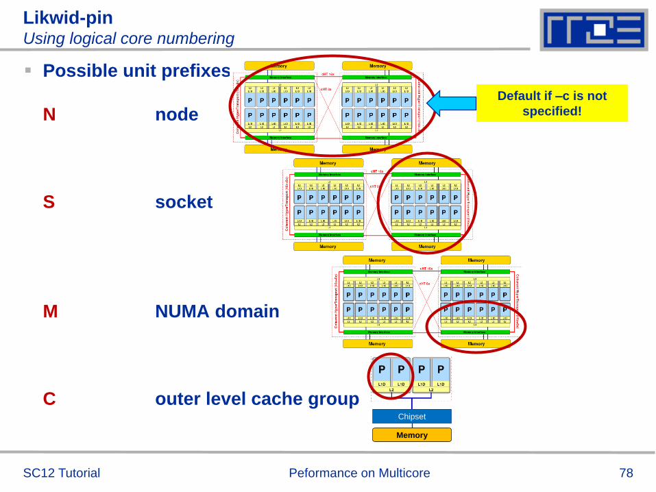
Likwid-pin Using logical core numbering

Possible unit prefixes

N node

S socket

M NUMA domain

C outer level cache group


Chipset

Memory

Default if –c is not

specified!

79

likwid-mpirun

MPI startup and Hybrid pinning

How do you manage affinity with MPI or hybrid MPI/threading?

In the long run a unified standard is needed

Till then, likwid-mpirun provides a portable/flexible solution

The examples here are for Intel MPI/OpenMP programs, but are

also applicable to other threading models

Pure MPI:

$ likwid-mpirun -np 16 -nperdomain S:2 ./a.out

Hybrid:

$ likwid-mpirun -np 16 -pin S0:0,1_S1:0,1 ./a.out


80

likwid-mpirun

1 MPI process per node

likwid-mpirun –np 2 -pin N:0-11 ./a.out

SC12 Tutorial

Intel MPI+compiler:

OMP_NUM_THREADS=12 mpirun –ppn 1 –np 2 –env KMP_AFFINITY scatter ./a.out


81

likwid-mpirun

1 MPI process per socket

likwid-mpirun –np 4 –pin S0:0-5_S1:0-5 ./a.out

SC12 Tutorial

Intel MPI+compiler: OMP_NUM_THREADS=6 mpirun –ppn 2 –np 4 \

–env I_MPI_PIN_DOMAIN socket –env KMP_AFFINITY scatter ./a.out


82

likwid-mpirun

Integration of likwid-perfctr

SC12 Tutorial

likwid-mpirun can optionally set up likwid-perfctr for you

$ likwid-mpirun –np 16 –nperdomain S:2 –perf FLOPS_DP \

-marker –mpi intelmpi ./a.out

likwid-mpirun generates an intermediate perl script which is called

by the native MPI start mechanism

According the MPI rank the script pins the process and threads

If you use perfctr after the run for each process a file in the format Perf-<hostname>-<rank>.txt

Its output which contains the perfctr results.

In the future analysis scripts will be added which generate reports

of the raw data (e.g. as html pages)


83

The Plan




processors



Micro-

bench

marks

Sync

over-

head

Band-

width

saturation




Part 1

Probing

topology

Enforcing

affinity


Balance

metrics

“Motivated”

optimizations

Case study:

3D Jacobi smoother

The Roofline Model

Hands-On session 1


ccNUMA nodes


(SMT)

Theory Impli-

cations

Facts &

fiction


Intranode vs.

internode

Rank-

subdomain

mapping


Part 2

Hardware

metrics

Best

practices



Wavefront

temporal

blocking

Sparse MVM

(part 2)

Outlook: Advanced


Sparse MVM

(part 3) ECM model

Conclusions

Hands-On session 2

SC12 Tutorial

84

The Plan




processors



Micro-

bench

marks

Sync

over-

head

Band-

width

saturation




Part 1

Probing

topology

Enforcing

affinity


Balance

metrics

“Motivated”

optimizations

Case study:

3D Jacobi smoother

The Roofline Model

Hands-On session 1


ccNUMA nodes


(SMT)

Theory Impli-

cations

Facts &

fiction


Intranode vs.

internode

Rank-

subdomain

mapping


Part 2

Hardware

metrics

Best

practices



Wavefront

temporal

blocking

Sparse MVM

(part 2)

Outlook: Advanced


Sparse MVM

(part 3) ECM model

Conclusions

Hands-On session 2

SC12 Tutorial

Basic performance modeling and

“motivated optimizations”

Machine and code balance

Example: The Jacobi smoother

The Roofline Model

86

Balance metric: Machine balance

The machine balance for data memory access of a specific computer

is given by

(architectural

limitation)

Bandwidth: 1 W = 8 bytes = 64 bits

bS = achievable bandwidth over

the slowest data path

Floating point peak: Pmax

Machine Balance = How many input operands can be delivered for

each FP operation?

Typical values (main memory): AMD Interlagos (2.3 GHz): Bm = {(17/8) GW/s} / {4 x 2.3 x 8 GFlop/s} ~0.029 W/F

Intel Sandy Bridge EP (2.7 GHz): ~0.025 W/F

NEC SX9 (vector): ~0.3 W/F

nVIDIA GTX480 ~0.026 W/F

]flops/s[

]words/s[

maxP

bB S

m


87

Machine Balance: Typical values beyond main memory

Data path Balance BM [W/F]

Cache 0.5 – 1.0

Machine (main memory) 0.01 – 0.5

Interconnect (Infiniband) 0.001 – 0.002

Interconnect (GBit ethernet) 0.0001 – 0.0007

Disk (or disk subsystem) 0.0001 – 0.001

1/BM = “Computational Intensity”: How many FP ops can be

performed before FP performance becomes a bottleneck?

Do

ub

le p

rec

isio

n:

W

64

-Bit


88

Balance metric: Code balance & lightspeed estimates

BM tells us what the hardware can deliver at most

Code balance (BC) quantifies

the requirements of the code:

Expected fraction of peak performance

(„lightspeed"):

l =1 code is not limited by bandwidth

Lightspeed for absolute performance:

(Pmax : “applicable” peak performance)

Example: Vector triad A(:)=B(:)+C(:)*D(:) on 2.3 GHz Interlagos

Bc = (4+1) Words / 2 Flops = 2.5 W/F (including write allocate)

Bm/Bc = 0.029/2.5 = 0.012, i.e. 1.2 % of peak performance (~1.7 GF/s)

][ operations arithmetic

][ (LD/ST) transfer data

flops

wordsBc

c

m

B

Bl ,1min

This is what we

need

This is what we

get

C

S

B

bPPlP ,min maxmax


89

Balance metric (a.k.a. the “roofline model”)

The balance metric formalism is based on some (crucial)

assumptions:

The code makes balanced use of MULT and ADD operation. For others

(e.g. A=B+C) the peak performance input parameter Pmax has to be

adjusted (e.g. Pmax Pmax/2 )

Attainable bandwidth of code = input parameter! Determine effective

bandwidth via simple streaming benchmarks to model more complex

kernels and applications.

Definition is based on 64-bit arithmetic but can easily be adjusted, e.g. for

32-bit

Data transfer and arithmetic overlap perfectly!

Slowest data path is modeled only; all others are assumed to be infinitely

fast

Latency effects are ignored, i.e. perfect streaming mode


90

Balance metric: 2D diffusion equation + Jacobi solver

Diffusion equation in 2D

Stationary solution with Dirichlet boundary conditions using

Jacobi iteration scheme can be obtained with:

Balance (crude estimate incl. write allocate):

phi(:,:,t0): 3 LD +

phi(:,:,t1): 1 ST+ 1LD

BC = 5 W / 4 FLOPs = 1.25 W / F

Reuse when computing phi(i+2,k,t1)

WRITE ALLOCATE: LD + ST phi(i,k,t1)


91

Balance metric: 2 D Jacobi

Modern cache subsystems may further reduce memory traffic

If cache is large enough to hold at least 2 rows (shaded region): Each phi(:,:,t0) is loaded

once from main memory and reused 3 times from

cache:

phi(:,:,t0): 1 LD + phi(:,:,t1): 1 ST+ 1LD

BC = 3 W / 4 F = 0.75 W / F

If cache is large enough to hold at least one row phi(:,k-1,t0) needs to be reloaded:

phi(:,:,t0): 2 LD + phi(:,:,t1): 1 ST+ 1LD

BC = 4 W / 4 F = 1.0 W / F

Beyond that: phi(:,:,t0): 2 LD + phi(:,:,t1): 1 ST+ 1LD

BC = 5 W / 4 F = 1.25 W / F


92

Performance metrics: 2D Jacobi

Alternative implementation (“Macho FLOP version”)

MFlops/sec increases by 7/4 but time to solution remains the same

Better metric (for many iterative stencil schemes):

Lattice Site Updates per Second (LUPs/sec)

2D Jacobi example: Compute LUPs/sec metric via


wall

maxmaxmax]/[T

kiitsMLUPsP

93

Balance metric for 3D Jacobi

3D sweep:

Best case balance: 1 LD phi(i,j,k+1,t0)

1 ST + 1 write allocate phi(i,j,k,t1)

6 flops

BC = 0.5 W/F (24 bytes/update)

No 2-layer condition but 2 rows fit: BC = 5/6 W/F (40 bytes/update)

Worst case (2 rows do not fit): BC = 7/6 W/F (56 bytes/update)


do k=1,kmax

do j=1,jmax

do i=1,imax

phi(i,j,k,t1) = oos *(phi(i-1,j,k,t0)+phi(i+1,j,k,t0) &

+ phi(i,j-1,k,t0)+phi(i,j+1,k,t0) &

+ phi(i,j,k-1,t0)+phi(i,j,k+1,t0))

enddo

enddo

enddo

94

3D Jacobi solver Performance of vanilla code on one Interlagos chip (8 cores)


cache memory

2 layers of source array

drop out of L2 cache

Problem size: N3

95

Conclusions from the Jacobi example

We have made sense of the memory-bound performance vs.

problem size

“Layer conditions” lead to predictions of code balance

Achievable memory bandwidth is input parameter

The model works only if the bandwidth is “saturated”

In-cache modeling is more involved

Optimization == reducing the code balance by code

transformations

See below


Data access optimizations

General considerations

Case study: Optimizing a Jacobi solver

97

Premise

Data access is the most prevalent

performance-limiting factor in computing



Data access – general considerations

Case 1: O(N)/O(N) Algorithms

O(N) arithmetic operations vs. O(N) data access operations

Examples: Scalar product, vector addition, sparse MVM etc.

Performance limited by memory BW for large N (“memory bound”)

Limited optimization potential for single loops

…at most a constant factor for multi-loop operations

Example: successive vector additions

do i=1,N

a(i)=b(i)+c(i)

enddo

do i=1,N

z(i)=b(i)+e(i)

enddo no optimization potential for either loop

do i=1,N

a(i)=b(i)+c(i)

z(i)=b(i)+e(i)

enddo

fusing different loops

allows O(N) data

reuse from registers

Loop fusion

Bc = 3/1 W/F

Bc = 5/2 W/F


Data access – general guidelines

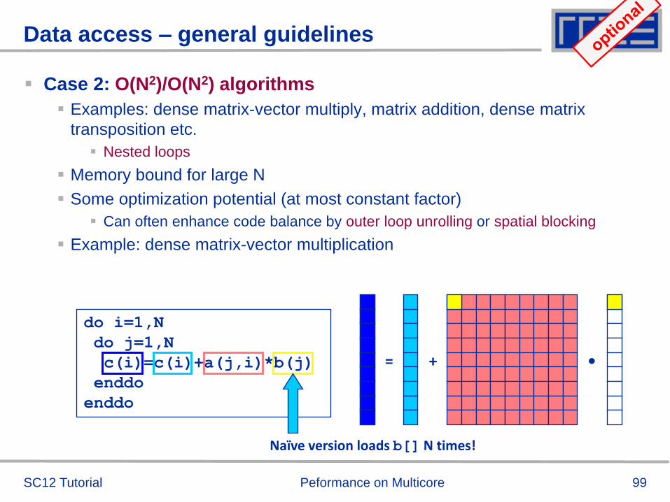
Case 2: O(N2)/O(N2) algorithms

Examples: dense matrix-vector multiply, matrix addition, dense matrix

transposition etc.

Nested loops

Memory bound for large N

Some optimization potential (at most constant factor)

Can often enhance code balance by outer loop unrolling or spatial blocking

Example: dense matrix-vector multiplication

do i=1,N

do j=1,N

c(i)=c(i)+a(j,i)*b(j)

enddo

enddo

= + •

Naïve version loads b[] N times!



O(N2)/O(N2) algorithms cont’d

“Unroll & jam” optimization (or “outer loop unrolling”)

do i=1,N

do j=1,N

c(i)=c(i)+a(j,i)*b(j)

enddo

enddo

do i=1,N,2

do j=1,N

c(i) =c(i) +a(j,i) *b(j)

enddo

do j=1,N

c(i+1)=c(i+1)+a(j,i+1)*b(j)

enddo

enddo

unroll

do i=1,N,2

do j=1,N

c(i) =c(i) +a(j,i) * b(j)

c(i+1)=c(i+1)+a(j,i+1)* b(j)

enddo

enddo

jam

b(j) can be re-used once

from register → save 1 LD

operation

Lowers Bc from 1 to ¾ W/F


O(N2)/O(N2) algorithms cont’d

Data access pattern for 2-way unrolled dense MVM:

Data transfers can further be reduced by more aggressive unrolling (i.e., m-

way instead of 2-way)

Significant code bloat (try to use compiler directives if possible)

Main memory limit: b[] only be loaded once from memory (Bc ≈ ½ W/F) (can be

achieved by high unrolling OR large outer level caches)

Outer loop unrolling can also be beneficial to reduce traffic within caches!

Beware: CPU registers are a limited resource

Excessive unrolling can cause register spills to memory


= + •

Vector b[] now only loaded

N/2 times!

Remainder loop handled

separately

Case study:

3D Jacobi solver

Spatial blocking for improved cache utilization

103

Remember the 3D Jacobi solver on Interlagos?


2 layers of source array

drop out of L2 cache

avoid through spatial

blocking!


Jacobi iteration (2D): No spatial Blocking

Assumptions:

cache can hold 32 elements (16 for each array)

Cache line size is 4 elements

Perfect eviction strategy for source array

This element is needed for three more updates; but 29 updates happen before this element is

used for the last time

i

k


Jacobi iteration (2D): No spatial blocking

Assumptions:

cache can hold 32 elements (16 for each array)

Cache line size is 4 elements

Perfect eviction strategy for source array

This element is needed for

three more updates but has

been evicted


Jacobi iteration (2D): Spatial Blocking

divide system into blocks

update block after block

same performance as if three complete rows of the systems fit

into cache


Jacobi iteration (2D): Spatial Blocking

Spatial blocking reorders traversal of data to account for the data

update rule of the code

Elements stay sufficiently long in cache to be fully reused

Spatial blocking improves temporal locality! (Continuous access in inner loop ensures spatial locality)

This element remains in cache until it is fully used (only 6 updates happen before

last use of this element)


Jacobi iteration (2D): Spatial blocking

Implementation:

Guidelines:

Blocking of inner loop levels (traversing continuously through main memory)

Blocking size iblock large enough to keep elements sufficiently long in

cache but cache size is a hard limit!

Blocking loops may have some impact on ccNUMA page placement (see

later)

do it=1,itmax

do ioffset=1,imax,iblock

do k=1,kmax

do i=ioffset, min(imax,ioffset+iblock-1)

phi(i, k, t1) = ( phi(i-1, k, t0) + phi(i+1, k, t0)

+ phi(i, k-1, t0) + phi(i, k+1, t0) )*0.25

enddo

enddo

enddo

enddo

loop over i-blocks

109

3D Jacobi solver (problem size 4003) Blocking different loop levels (8 cores Interlagos)


3D vs. 2D?

OpenMP parallelization?

Optimal block size?

k-loop blocking?

see Exercise!

24B/update

performance

model

inner (i) loop

blocking

middle (j) loop

blocking

optimum j

block size

110

3D Jacobi solver Spatial blocking + nontemporal stores


blocking NT

stores

expected

boost:

50%

16 B/update perf. model

The Roofline Model

112

The Roofline Model – A tool for more insight

1. Determine the applicable peak performance of a loop, assuming

that data comes from L1 cache

2. Determine the computational intensity (flops per byte

transferred) over the slowest data path utilized (1/Bc)

3. Determine the applicable peak bandwidth of the slowest data

path utilized

Example: do i=1,N; s=s+a(i); enddo

in DP on hypothetical CPU, N large

ADD peak (half of full peak)

4-cycle latency per ADD if not unrolled

Computational intensity (= 1/Bc)

Expected

performance


113

Input to the roofline model

… on the example of do i=1,N; s=s+a(i); enddo


analysis

Code analysis:

1 ADD + 1 LOAD

architecture

Throughput: 1 ADD + 1 LD/cy

Pipeline depth: 4 cy (ADD)

measurement

Maximum memory

bandwidth 10 GB/s

Memory-bound @ large N!

Pmax = 1.25 GF/s

114

Factors to consider in the roofline model

Bandwidth-bound (simple case)

Accurate traffic calculation (write-

allocate, strided access, …)

Practical ≠ theoretical BW limits

Erratic access patterns

Core-bound (may be complex)

Multiple bottlenecks: LD/ST,

arithmetic, pipelines, SIMD,

execution ports

Still probably some contributions

from data access


115

Example: SpMVM node performance model

Sparse MVM in

double precision w/ CRS:

DP CRS code balance

quantifies extra traffic

for loading RHS more than

once

Predicted Performance = streamBW/BCRS

Determine by measuring performance and actual memory bandwidth

8 8 8 4 8

8

G. Schubert, G. Hager, H. Fehske and G. Wellein: Parallel sparse matrix-vector multiplication as a test case

for hybrid MPI+OpenMP programming. Workshop on Large-Scale Parallel Processing (LSPP 2011), May 20th,

2011, Anchorage, AK. DOI:10.1109/IPDPS.2011.332, Preprint: arXiv:1101.0091


http://dx.doi.org/10.1109/IPDPS.2011.332

http://arxiv.org/abs/1101.0091

116

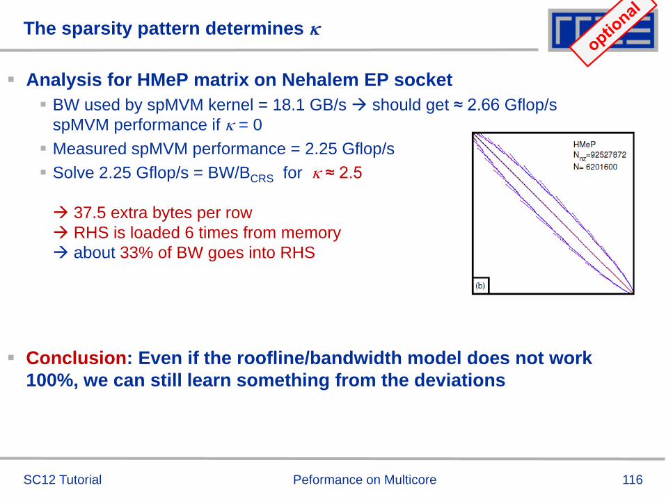
The sparsity pattern determines

Analysis for HMeP matrix on Nehalem EP socket

BW used by spMVM kernel = 18.1 GB/s should get ≈ 2.66 Gflop/s

spMVM performance if = 0

Measured spMVM performance = 2.25 Gflop/s

Solve 2.25 Gflop/s = BW/BCRS for ≈ 2.5

37.5 extra bytes per row

RHS is loaded 6 times from memory

about 33% of BW goes into RHS

Conclusion: Even if the roofline/bandwidth model does not work

100%, we can still learn something from the deviations


117

Input to the roofline model

… on the example of spMVM with HMeP matrix

Code analysis:

1 ADD, 1 MULT,

(2.5+2/Nnzr) LOADs,

1/Nnzr STOREs +

Throughput: 1 ADD, 1 MULT

+ 1 LD + 1ST/cy

Maximum memory

bandwidth 20 GB/s

Memory-bound!

= 2.5

Measured memory BW

for spMVM 18.1 GB/s


118

Assumptions and shortcomings of the roofline model

Assumes one of two bottlenecks

1. In-core execution

2. Bandwidth of a single hierarchy level

Latency effects are not modeled pure data streaming assumed

In-core execution is sometimes hard to

model

Saturation effects in multicore

chips are not explained

ECM model gives more insight

(see later)

A(:)=B(:)+C(:)*D(:)

Roofline predicts

full socket BW


119

The Plan




processors



Micro-

bench

marks

Sync

over-

head

Band-

width

saturation




Part 1

Probing

topology

Enforcing

affinity


Balance

metrics

“Motivated”

optimizations

Case study:

3D Jacobi smoother

The Roofline Model

Hands-On session 1


ccNUMA nodes


(SMT)

Theory Impli-

cations

Facts &

fiction


Intranode vs.

internode

Rank-

subdomain

mapping


Part 2

Hardware

metrics

Best

practices



Wavefront

temporal

blocking

Sparse MVM

(part 2)

Outlook: Advanced


Sparse MVM

(part 3) ECM model

Conclusions

Hands-On session 2

SC12 Tutorial

Efficient parallel programming

on ccNUMA nodes

Performance characteristics of ccNUMA nodes

First touch placement policy

C++ issues

ccNUMA locality and dynamic scheduling

ccNUMA locality beyond first touch


ccNUMA performance problems “The other affinity” to care about

ccNUMA:

Whole memory is transparently accessible by all processors

but physically distributed

with varying bandwidth and latency

and potential contention (shared memory paths)

How do we make sure that memory access is always as "local"

and "distributed" as possible?

Page placement is implemented in units of OS pages (often 4kB, possibly

more)

C C C C

M M

C C C C

M M

122

Cray XE6 Interlagos node

4 chips, two sockets, 8 threads per ccNUMA domain

ccNUMA map: Bandwidth penalties for remote access

Run 8 threads per ccNUMA domain (1 chip)

Place memory in different domain 4x4 combinations

STREAM triad benchmark using nontemporal stores


ST

RE

AM

tri

ad

pe

rfo

rma

nc

e [

MB

/s]

Memory node

CP

U n

od

e


ccNUMA locality tool numactl:

How do we enforce some locality of access?

numactl can influence the way a binary maps its memory pages:

numactl --membind=<nodes> a.out # map pages only on <nodes>

--preferred=<node> a.out # map pages on <node>

# and others if <node> is full

--interleave=<nodes> a.out # map pages round robin across

# all <nodes>

Examples:

env OMP_NUM_THREADS=2 numactl --membind=0 --cpunodebind=1 ./stream

env OMP_NUM_THREADS=4 numactl --interleave=0-3 \

likwid-pin -c N:0,4,8,12 ./stream

But what is the default without numactl?


ccNUMA default memory locality

"Golden Rule" of ccNUMA:

A memory page gets mapped into the local memory of the

processor that first touches it!

Except if there is not enough local memory available

This might be a problem, see later

Caveat: "touch" means "write", not "allocate"

Example:

double *huge = (double*)malloc(N*sizeof(double));

for(i=0; i<N; i++) // or i+=PAGE_SIZE

huge[i] = 0.0;

It is sufficient to touch a single item to map the entire page

Memory not

mapped here yet

Mapping takes

place here


Coding for ccNUMA data locality

integer,parameter :: N=10000000

double precision A(N), B(N)

A=0.d0

!$OMP parallel do

do i = 1, N

B(i) = function ( A(i) )

end do



double precision A(N),B(N)

!$OMP parallel

!$OMP do schedule(static)

do i = 1, N

A(i)=0.d0

end do

!$OMP end do

...


do i = 1, N


end do

!$OMP end do

!$OMP end parallel

Most simple case: explicit initialization


Coding for ccNUMA data locality


double precision A(N), B(N)

READ(1000) A

!$OMP parallel do

do i = 1, N


end do



double precision A(N),B(N)

!$OMP parallel


do i = 1, N

A(i)=0.d0

end do

!$OMP end do

!$OMP single

READ(1000) A

!$OMP end single


do i = 1, N


end do

!$OMP end do

!$OMP end parallel

Sometimes initialization is not so obvious: I/O cannot be easily

parallelized, so “localize” arrays before I/O


Coding for Data Locality

Required condition: OpenMP loop schedule of initialization must

be the same as in all computational loops

Only choice: static! Specify explicitly on all NUMA-sensitive loops, just to

be sure…

Imposes some constraints on possible optimizations (e.g. load balancing)

Presupposes that all worksharing loops with the same loop length have the

same thread-chunk mapping

Guaranteed by OpenMP 3.0 only for loops in the same enclosing parallel region

and static schedule

In practice, it works with any compiler even across regions

If dynamic scheduling/tasking is unavoidable, more advanced methods may

be in order

How about global objects?

Better not use them

If communication vs. computation is favorable, might consider properly

placed copies of global data

In C++, STL allocators provide an elegant solution (see hidden slides)


Coding for Data Locality:

Placement of static arrays or arrays of objects

Speaking of C++: Don't forget that constructors tend to touch the

data members of an object. Example:

class D { double d;

public:

D(double _d=0.0) throw() : d(_d) {}

inline D operator+(const D& o) throw() {

return D(d+o.d);

}

inline D operator*(const D& o) throw() {

return D(d*o.d);

}

...

};

→ placement problem with D* array = new D[1000000];


Coding for Data Locality:

Parallel first touch for arrays of objects

Solution: Provide overloaded D::operator new[]

Placement of objects is then done automatically by the C++ runtime via

“placement new”

void* D::operator new[](size_t n) {

char *p = new char[n]; // allocate

size_t i,j;

#pragma omp parallel for private(j) schedule(...)

for(i=0; i<n; i += sizeof(D))

for(j=0; j<sizeof(D); ++j)

p[i+j] = 0;

return p;

}

void D::operator delete[](void* p) throw() {

delete [] static_cast<char*>p;

}

parallel first

touch


Coding for Data Locality: NUMA allocator for parallel first touch in std::vector<>

template <class T> class NUMA_Allocator {

public:

T* allocate(size_type numObjects, const void

*localityHint=0) {

size_type ofs,len = numObjects * sizeof(T);

void *m = malloc(len);

char *p = static_cast<char*>(m);

int i,pages = len >> PAGE_BITS;

#pragma omp parallel for schedule(static) private(ofs)

for(i=0; i<pages; ++i) {

ofs = static_cast<size_t>(i) << PAGE_BITS;

p[ofs]=0;

}

return static_cast<pointer>(m);

}

...

}; Application: vector<double,NUMA_Allocator<double> > x(10000000)


Diagnosing Bad Locality

If your code is cache-bound, you might not notice any locality

problems

Otherwise, bad locality limits scalability at very low CPU numbers

(whenever a node boundary is crossed)

If the code makes good use of the memory interface

But there may also be a general problem in your code…

Consider using performance counters

LIKWID-perfctr can be used to measure nonlocal memory accesses

Example for Intel Nehalem (Core i7):

env OMP_NUM_THREADS=8 likwid-perfctr -g MEM –C N:0-7 \

-t intel ./a.out


Using performance counters for diagnosing bad ccNUMA

access locality

Intel Nehalem EP node:

+-------------------------------+-------------+-------------+-------------+-------------+-------------+-------------+-------------+-------------+

| Event | core 0 | core 1 | core 2 | core 3 | core 4 | core 5 | core 6 | core 7 |

+-------------------------------+-------------+-------------+-------------+-------------+-------------+-------------+-------------+-------------+

| INSTR_RETIRED_ANY | 5.20725e+08 | 5.24793e+08 | 5.21547e+08 | 5.23717e+08 | 5.28269e+08 | 5.29083e+08 | 5.30103e+08 | 5.29479e+08 |

| CPU_CLK_UNHALTED_CORE | 1.90447e+09 | 1.90599e+09 | 1.90619e+09 | 1.90673e+09 | 1.90583e+09 | 1.90746e+09 | 1.90632e+09 | 1.9071e+09 |

| UNC_QMC_NORMAL_READS_ANY | 8.17606e+07 | 0 | 0 | 0 | 8.07797e+07 | 0 | 0 | 0 |

| UNC_QMC_WRITES_FULL_ANY | 5.53837e+07 | 0 | 0 | 0 | 5.51052e+07 | 0 | 0 | 0 |

| UNC_QHL_REQUESTS_REMOTE_READS | 6.84504e+07 | 0 | 0 | 0 | 6.8107e+07 | 0 | 0 | 0 |

| UNC_QHL_REQUESTS_LOCAL_READS | 6.82751e+07 | 0 | 0 | 0 | 6.76274e+07 | 0 | 0 | 0 |

+-------------------------------+-------------+-------------+-------------+-------------+-------------+-------------+-------------+-------------+

RDTSC timing: 0.827196 s

+-----------------------------+----------+----------+---------+----------+----------+----------+---------+---------+

| Metric | core 0 | core 1 | core 2 | core 3 | core 4 | core 5 | core 6 | core 7 |

+-----------------------------+----------+----------+---------+----------+----------+----------+---------+---------+

| Runtime [s] | 0.714167 | 0.714733 | 0.71481 | 0.715013 | 0.714673 | 0.715286 | 0.71486 | 0.71515 |

| CPI | 3.65735 | 3.63188 | 3.65488 | 3.64076 | 3.60768 | 3.60521 | 3.59613 | 3.60184 |

| Memory bandwidth [MBytes/s] | 10610.8 | 0 | 0 | 0 | 10513.4 | 0 | 0 | 0 |

| Remote Read BW [MBytes/s] | 5296 | 0 | 0 | 0 | 5269.43 | 0 | 0 | 0 |

+-----------------------------+----------+----------+---------+----------+----------+----------+---------+---------+

Uncore events only

counted once per socket

Half of read BW comes

from other socket!


If all fails…

Even if all placement rules have been carefully observed, you may

still see nonlocal memory traffic. Reasons?

Program has erratic access patters may still achieve some access

parallelism (see later)

OS has filled memory with buffer cache data:

# numactl --hardware # idle node!

available: 2 nodes (0-1)


node 0 free: 906 MB



top - 14:18:25 up 92 days, 6:07, 2 users, load average: 0.00, 0.02, 0.00

Mem: 4065564k total, 1149400k used, 2716164k free, 43388k buffers

Swap: 2104504k total, 2656k used, 2101848k free, 1038412k cached


ccNUMA problems beyond first touch:

Buffer cache

OS uses part of main memory for

disk buffer (FS) cache

If FS cache fills part of memory,

apps will probably allocate from

foreign domains

non-local access!

“sync” is not sufficient to

drop buffer cache blocks

Remedies

Drop FS cache pages after user job has run (admin’s job)

seems to be automatic after aprun has finished on Crays

User can run “sweeper” code that allocates and touches all physical

memory before starting the real application

numactl tool or aprun can force local allocation (where applicable)

Linux: There is no way to limit the buffer cache size in standard kernels

P1 C

P2 C

C C

MI

P3 C

P4 C

C C

MI

BC

data(3)

BC

data(3)

data

(1)


ccNUMA problems beyond first touch:

Buffer cache

Real-world example: ccNUMA and the Linux buffer cache

Benchmark:

1. Write a file of some size

from LD0 to disk

2. Perform bandwidth

benchmark using

all cores in LD0 and

maximum memory

installed in LD0

Result: By default,

Buffer cache is given

priority over local

page placement

restrict to local

domain if possible!

aprun –ss ...

(Cray only)


ccNUMA placement and erratic access patterns

Sometimes access patterns are

just not nicely grouped into

contiguous chunks:

In both cases page placement cannot easily be fixed for perfect parallel

access

double precision :: r, a(M)

!$OMP parallel do private(r)

do i=1,N

call RANDOM_NUMBER(r)

ind = int(r * M) + 1

res(i) = res(i) + a(ind)

enddo

!OMP end parallel do

Or you have to use tasking/dynamic

scheduling:

!$OMP parallel

!$OMP single

do i=1,N

call RANDOM_NUMBER(r)

if(r.le.0.5d0) then

!$OMP task

call do_work_with(p(i))

!$OMP end task

endif

enddo

!$OMP end single

!$OMP end parallel


ccNUMA placement and erratic access patterns

Worth a try: Interleave memory across ccNUMA domains to get at least

some parallel access

1. Explicit placement:

2. Using global control via numactl:

numactl --interleave=0-3 ./a.out

Fine-grained program-controlled placement via libnuma (Linux)

using, e.g., numa_alloc_interleaved_subset(),

numa_alloc_interleaved() and others

!$OMP parallel do schedule(static,512)

do i=1,M

a(i) = …

enddo


This is for all memory, not

just the problematic

arrays!

Observe page alignment of

array to get proper

placement!

138

The curse and blessing of interleaved placement:

OpenMP STREAM on a Cray XE6 Interlagos node

Parallel init: Correct parallel initialization

LD0: Force data into LD0 via numactl –m 0

Interleaved: numactl --interleave <LD range>


139

The Plan




processors



Micro-

bench

marks

Sync

over-

head

Band-

width

saturation




Part 1

Probing

topology

Enforcing

affinity


Balance

metrics

“Motivated”

optimizations

Case study:

3D Jacobi smoother

The Roofline Model

Hands-On session 1


ccNUMA nodes


(SMT)

Theory Impli-

cations

Facts &

fiction


Intranode vs.

internode

Rank-

subdomain

mapping


Part 2

Hardware

metrics

Best

practices



Wavefront

temporal

blocking

Sparse MVM

(part 2)

Outlook: Advanced


Sparse MVM

(part 3) ECM model

Conclusions

Hands-On session 2

SC12 Tutorial

Simultaneous multithreading (SMT)

Principles and performance impact

SMT vs. independent instruction streams

Facts and fiction


SMT Makes a single physical core appear as two or more

“logical” cores multiple threads/processes run concurrently

SMT principle (2-way example):

Sta

nd

ard

co

re

2-w

ay S

MT


SMT impact

SMT is primarily suited for increasing processor throughput

With multiple threads/processes running concurrently

Scientific codes tend to utilize chip resources quite well

Standard optimizations (loop fusion, blocking, …)

High data and instruction-level parallelism

Exceptions do exist

SMT is an important topology issue

SMT threads share almost all core

resources

Pipelines, caches, data paths

Affinity matters!

If SMT is not needed

pin threads to physical cores

or switch it off via BIOS etc.

C C

C C

C C

C C

C C

C C

C

MI

Memory

P T0

T1

P T0

T1

P T0

T1

P T0

T1

P T0

T1

P T0

T1

P T0

T1

Th

read

0

Th

read

1

Th

read

2

C C

C C

C C

C C

C C

C C

C

MI

Memory

P T0

T1

P T0

T1

P T0

T1

P T0

T1

P T0

T1

P T0

T1

P T0

T1

Th

read

0

Th

read

1

Th

read

2


SMT impact

SMT adds another layer of topology

(inside the physical core)

Caveat: SMT threads share all caches!

Possible benefit: Better pipeline throughput

Filling otherwise unused pipelines

Filling pipeline bubbles with other thread’s executing instructions:

Beware: Executing it all in a single thread

(if possible) may reach the same goal

without SMT:

Thread 0: do i=1,N

a(i) = a(i-1)*c

enddo

Dependency pipeline

stalls until previous MULT

is over

Westmere EP

C C

C C

C C

C C

C C

C C

C

MI

Memory

P T0

T1

P T0

T1

P T0

T1

P T0

T1

P T0

T1

P T0

T1

P T0

T1

Thread 1: do i=1,N

b(i) = func(i)*d

enddo

Unrelated work in other

thread can fill the pipeline

bubbles

do i=1,N

a(i) = a(i-1)*c

b(i) = func(i)*d

enddo

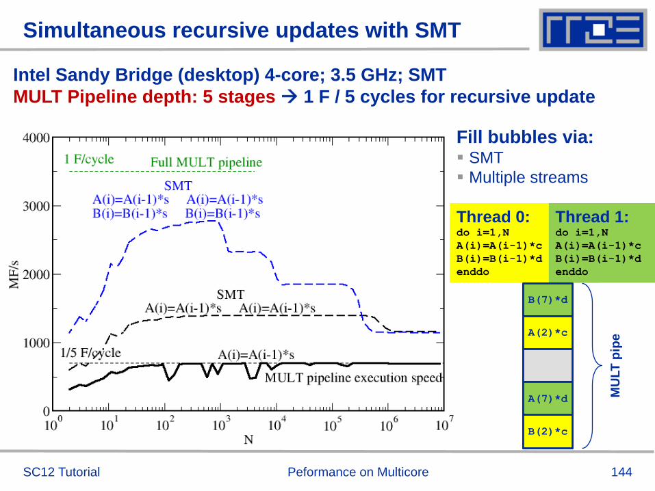
144

a(2)*c

Thread 0: do i=1,N

a(i)=a(i-1)*c

enddo

a(2)*c

a(7)*c

Thread 0: do i=1,N

a(i)=a(i-1)*c

enddo

Thread 1: do i=1,N

a(i)=a(i-1)*c

enddo

B(7)*d

A(2)*c

A(7)*d

B(2)*c

Thread 0: do i=1,N

A(i)=A(i-1)*c

B(i)=B(i-1)*d

enddo

Thread 1: do i=1,N

A(i)=A(i-1)*c

B(i)=B(i-1)*d

enddo

Simultaneous recursive updates with SMT


Intel Sandy Bridge (desktop) 4-core; 3.5 GHz; SMT

MULT Pipeline depth: 5 stages 1 F / 5 cycles for recursive update

Fill bubbles via: SMT

Multiple streams

MU

LT

pip

e

145




MULT Pipeline depth: 5 stages 1 F / 5 cycles for recursive update

5 independent updates on a single thread do the same job!

B(2)*s

A(2)*s

E(1)*s

D(1)*s

C(1)*s

Thread 0: do i=1,N

A(i)=A(i-1)*s

B(i)=B(i-1)*s

C(i)=C(i-1)*s

D(i)=D(i-1)*s

E(i)=E(i-1)*s

enddo

MU

LT

pip

e

146




Pure update benchmark can be vectorized 2 F / cycle (store limited)

Recursive update:

SMT can fill pipeline

bubles

A single thread can

do so as well

Bandwidth does not

increase through

SMT

SMT can not

replace SIMD!

147

SMT myths: Facts and fiction (1)

Myth: “If the code is compute-bound, then the functional units

should be saturated and SMT should show no improvement.”

Truth

1. A compute-bound loop does not

necessarily saturate the pipelines;

dependencies can cause a lot of bubbles,

which may be filled by SMT threads.

2. If a pipeline is already full, SMT will not improve its

utilization


B(7)*d

A(2)*c

A(7)*d

B(2)*c

Thread 0: do i=1,N

A(i)=A(i-1)*c

B(i)=B(i-1)*d

enddo

Thread 1: do i=1,N

A(i)=A(i-1)*c

B(i)=B(i-1)*d

enddo

MU

LT

pip

e

148


Myth: “If the code is memory-bound, SMT should help because it

can fill the bubbles left by waiting for data from memory.”

Truth:

1. If the maximum memory bandwidth is already reached, SMT will not

help since the relevant

resource (bandwidth)

is exhausted.

2. If the relevant

bottleneck is not

exhausted, SMT may

help since it can fill

bubbles in the LOAD

pipeline.

This applies also to other

“relevant bottlenecks!”


149


Myth: “SMT can help bridge the latency to

memory (more outstanding references).”

Truth: Outstanding references may or may not be

bound to SMT threads; they may be a resource

of the memory interface and shared by all

threads. The benefit of SMT with memory-bound

code is usually due to better utilization of the

pipelines so that less time gets “wasted” in the

cache hierarchy.

See also the “ECM Performance Model”

later on.



SMT: When it may help, and when not

Functional parallelization

FP-only parallel loop code

Frequent thread synchronization

Code sensitive to cache size

Strongly memory-bound code

Independent pipeline-unfriendly instruction streams

151

The Plan




processors



Micro-

bench

marks

Sync

over-

head

Band-

width

saturation




Part 1

Probing

topology

Enforcing

affinity


Balance

metrics

“Motivated”

optimizations

Case study:

3D Jacobi smoother

The Roofline Model

Hands-On session 1


ccNUMA nodes


(SMT)

Theory Impli-

cations

Facts &

fiction


Intranode vs.

internode

Rank-

subdomain

mapping


Part 2

Hardware

metrics

Best

practices



Wavefront

temporal

blocking

Sparse MVM

(part 2)

Outlook: Advanced


Sparse MVM

(part 3) ECM model

Conclusions

Hands-On session 2

SC12 Tutorial

Understanding MPI communication in

multicore environments

Intra-node vs. inter-node MPI

MPI Cartesian topologies and rank-subdomain

mapping

153

Intranode MPI

Common misconception: Intranode MPI is infinitely fast compared

to internode

Reality

Intranode latency is much smaller than internode

Intranode asymptotic bandwidth is surprisingly comparable to internode

Difference in saturation behavior

Other issues

Mapping between ranks, subdomains and cores with Cartesian MPI

topologies

Overlapping intranode with internode communication


154

MPI and Multicores

Clusters: Unidirectional internode Ping-Pong bandwidth

QDR/GBit ~ 30X


155

MPI and Multicores

Clusters: Unidirectional intranode Ping-Pong bandwidth

Mapping problem for most efficient communication paths!?

P C C

P C C

P C C

MI

P C C

C

Memory Memory

P C C

P C C

P C C

MI

P C C

C

Cross-Socket (CS)

Intra-Socket (IS)

Single point-to-

point BW similar

to internode

Some BW

scalability for

multi-intranode

connections


156

“Best possible” MPI:

Minimizing cross-node communication

■ Example: Stencil solver with halo exchange

■ Goal: Reduce inter-node halo traffic

■ Subdomains exchange halo with neighbors

■ Populate a node's ranks with “maximum neighboring” subdomains

■ This minimizes a node's communication surface

■ Shouldn’t MPI_CART_CREATE (w/ reorder) take care of this?


157

MPI rank-subdomain mapping in Cartesian topologies:

A 3D stencil solver and the growing number of cores per node

“Common” MPI

library behavior

Neh

ale

m E

P 2

-so

cket

Ista

nb

ul 2

-so

cket

Sh

an

gh

ai 4

-so

cket

Mag

ny C

ou

rs 2

-so

cket

Nehalem EX

4-socket

Magny Cours

4-socket

Wo

od

cre

st

2-s

ocket

Su

n N

iag

ara

2


158

~ 1.5x

4 ppn SDR-IB

MPI rank-subdomain mapping:

3D stencil solver – measurements for 8ppn and 4ppn GBE vs. IB

8 ppn QDR-IB

32 MPI processes


159

Summary on MPI multicore issues

Intranode MPI

May not be as fast as you think…

Becomes more important as core counts increase

May not be handled optimally by your MPI library

Rank-core mapping may be crucial for best performance

Reduce inter-node traffic

Most MPIs do not recognize this

Some (e.g., Cray) can give you hints toward optimal placement


160

The Plan




processors



Micro-

bench

marks

Sync

over-

head

Band-

width

saturation




Part 1

Probing

topology

Enforcing

affinity


Balance

metrics

“Motivated”

optimizations

Case study:

3D Jacobi smoother

The Roofline Model

Hands-On session 1


ccNUMA nodes


(SMT)

Theory Impli-

cations

Facts &

fiction


Intranode vs.

internode

Rank-

subdomain

mapping


Part 2

Hardware

metrics

Best

practices



Wavefront

temporal

blocking

Sparse MVM

(part 2)

Outlook: Advanced


Sparse MVM

(part 3) ECM model

Conclusions

Hands-On session 2

SC12 Tutorial

Best practices for using

hardware performance

metrics

likwid-perfctr


Probing performance behavior

How do we find out about the performance properties and

requirements of a parallel code?

Profiling via advanced tools is often overkill

A coarse overview is often sufficient

likwid-perfctr (similar to “perfex” on IRIX, “hpmcount” on AIX, “lipfpm” on

Linux/Altix)

Simple end-to-end measurement of hardware performance metrics

Operating modes:

Wrapper

Stethoscope

Timeline

Marker API

Preconfigured and extensible

metric groups, list with likwid-perfctr -a

BRANCH: Branch prediction miss rate/ratio

CACHE: Data cache miss rate/ratio

CLOCK: Clock of cores

DATA: Load to store ratio

FLOPS_DP: Double Precision MFlops/s

FLOPS_SP: Single Precision MFlops/s

FLOPS_X87: X87 MFlops/s

L2: L2 cache bandwidth in MBytes/s

L2CACHE: L2 cache miss rate/ratio

L3: L3 cache bandwidth in MBytes/s

L3CACHE: L3 cache miss rate/ratio

MEM: Main memory bandwidth in MBytes/s

TLB: TLB miss rate/ratio


likwid-perfctr

Example usage with preconfigured metric group

$ env OMP_NUM_THREADS=4 likwid-perfctr -C N:0-3 –t intel -g FLOPS_DP ./stream.exe

-------------------------------------------------------------

CPU type: Intel Core Lynnfield processor

CPU clock: 2.93 GHz

-------------------------------------------------------------

Measuring group FLOPS_DP

-------------------------------------------------------------

YOUR PROGRAM OUTPUT

+--------------------------------------+-------------+-------------+-------------+-------------+

| Event | core 0 | core 1 | core 2 | core 3 |

+--------------------------------------+-------------+-------------+-------------+-------------+

| INSTR_RETIRED_ANY | 1.97463e+08 | 2.31001e+08 | 2.30963e+08 | 2.31885e+08 |

| CPU_CLK_UNHALTED_CORE | 9.56999e+08 | 9.58401e+08 | 9.58637e+08 | 9.57338e+08 |

| FP_COMP_OPS_EXE_SSE_FP_PACKED | 4.00294e+07 | 3.08927e+07 | 3.08866e+07 | 3.08904e+07 |

| FP_COMP_OPS_EXE_SSE_FP_SCALAR | 882 | 0 | 0 | 0 |

| FP_COMP_OPS_EXE_SSE_SINGLE_PRECISION | 0 | 0 | 0 | 0 |

| FP_COMP_OPS_EXE_SSE_DOUBLE_PRECISION | 4.00303e+07 | 3.08927e+07 | 3.08866e+07 | 3.08904e+07 |

+--------------------------------------+-------------+-------------+-------------+-------------+

+--------------------------+------------+---------+----------+----------+

| Metric | core 0 | core 1 | core 2 | core 3 |

+--------------------------+------------+---------+----------+----------+

| Runtime [s] | 0.326242 | 0.32672 | 0.326801 | 0.326358 |

| CPI | 4.84647 | 4.14891 | 4.15061 | 4.12849 |

| DP MFlops/s (DP assumed) | 245.399 | 189.108 | 189.024 | 189.304 |

| Packed MUOPS/s | 122.698 | 94.554 | 94.5121 | 94.6519 |

| Scalar MUOPS/s | 0.00270351 | 0 | 0 | 0 |

| SP MUOPS/s | 0 | 0 | 0 | 0 |

| DP MUOPS/s | 122.701 | 94.554 | 94.5121 | 94.6519 |

+--------------------------+------------+---------+----------+----------+

Always

measured

Derived

metrics

Configured metrics

(this group)

164

likwid-perfctr Best practices for runtime counter analysis

Things to look at (in roughly this

order)

Load balance (flops, instructions,

BW)

In-socket memory BW saturation

Shared cache BW saturation

Flop/s, loads and stores per flop

metrics

SIMD vectorization

CPI metric

# of instructions,

branches, mispredicted branches

Caveats

Load imbalance may not show in

CPI or # of instructions Spin loops in OpenMP barriers/MPI

blocking calls

Looking at “top” or the Windows Task

Manager does not tell you anything useful

In-socket performance saturation

may have various reasons

Cache miss metrics are overrated

If I really know my code, I can often

calculate the misses

Runtime and resource utilization is

much more important


165

likwid-perfctr

Identify load imbalance…

Instructions retired / CPI may not be a good indication of

useful workload – at least for numerical / FP intensive codes….

Floating Point Operations Executed is often a better indicator

Waiting / “Spinning” in barrier generates a high instruction count

!$OMP PARALLEL DO

DO I = 1, N

DO J = 1, I

x(I) = x(I) + A(J,I) * y(J)

ENDDO

ENDDO

!$OMP END PARALLEL DO


166

likwid-perfctr

… and load-balanced codes

!$OMP PARALLEL DO

DO I = 1, N

DO J = 1, N

x(I) = x(I) + A(J,I) * y(J)

ENDDO

ENDDO


Higher CPI but

better performance

env OMP_NUM_THREADS=6 likwid-perfctr –t intel –C S0:0-5 –g FLOPS_DP ./a.out


167

likwid-perfctr counts events on cores; it has no notion of what

kind of code is running (if any)

This enables to listen on what currently happens without any

overhead:

likwid-perfctr -c N:0-11 -g FLOPS_DP -s 10

It can be used as cluster/server monitoring tool

A frequent use is to measure a certain part of a long running

parallel application from outside

SC12 Tutorial

likwid-perfctr

Stethoscope mode


168

likwid-perfctr

Timeline mode

likwid-perfctr supports time resolved measurements of full node:

likwid-perfctr –c N:0-11 -g MEM –d 50ms > out.txt


169

likwid-perfctr

Marker API

To measure only parts of an application a marker API is available.

The API only turns counters on/off. The configuration of the

counters is still done by likwid-perfctr application.

Multiple named regions can be measured

Results on multiple calls are accumulated

Inclusive and overlapping Regions are allowed

SC12 Tutorial

likwid_markerInit(); // must be called from serial region

likwid_markerStartRegion(“Compute”);

. . .

likwid_markerStopRegion(“Compute”);

likwid_markerStartRegion(“postprocess”);

. . .

likwid_markerStopRegion(“postprocess”);

likwid_markerClose(); // must be called from serial region


170

likwid-perfctr

Group files

SHORT PSTI

EVENTSET

FIXC0 INSTR_RETIRED_ANY

FIXC1 CPU_CLK_UNHALTED_CORE

FIXC2 CPU_CLK_UNHALTED_REF

PMC0 FP_COMP_OPS_EXE_SSE_FP_PACKED

PMC1 FP_COMP_OPS_EXE_SSE_FP_SCALAR

PMC2 FP_COMP_OPS_EXE_SSE_SINGLE_PRECISION

PMC3 FP_COMP_OPS_EXE_SSE_DOUBLE_PRECISION

UPMC0 UNC_QMC_NORMAL_READS_ANY

UPMC1 UNC_QMC_WRITES_FULL_ANY

UPMC2 UNC_QHL_REQUESTS_REMOTE_READS

UPMC3 UNC_QHL_REQUESTS_LOCAL_READS

METRICS

Runtime [s] FIXC1*inverseClock

CPI FIXC1/FIXC0

Clock [MHz] 1.E-06*(FIXC1/FIXC2)/inverseClock

DP MFlops/s (DP assumed) 1.0E-06*(PMC0*2.0+PMC1)/time

Packed MUOPS/s 1.0E-06*PMC0/time

Scalar MUOPS/s 1.0E-06*PMC1/time

SP MUOPS/s 1.0E-06*PMC2/time

DP MUOPS/s 1.0E-06*PMC3/time

Memory bandwidth [MBytes/s] 1.0E-06*(UPMC0+UPMC1)*64/time;

Remote Read BW [MBytes/s] 1.0E-06*(UPMC2)*64/time;

LONG

Formula:

DP MFlops/s = (FP_COMP_OPS_EXE_SSE_FP_PACKED*2 + FP_COMP_OPS_EXE_SSE_FP_SCALAR)/ runtime.

SC12 Tutorial

Groups are architecture-specific

They are defined in simple text files

Code is generated on recompile of

likwid

likwid-perfctr -a outputs list of groups

For every group an extensive

documentation is available


Measuring energy consumption

with LIKWID

172

Measuring energy consumption

likwid-powermeter and likwid-perfctr -g ENERGY

Implements Intel RAPL interface (Sandy Bridge)

RAPL = “Running average power limit” -------------------------------------------------------------

CPU name: Intel Core SandyBridge processor

CPU clock: 3.49 GHz

-------------------------------------------------------------

Base clock: 3500.00 MHz

Minimal clock: 1600.00 MHz

Turbo Boost Steps:

C1 3900.00 MHz

C2 3800.00 MHz

C3 3700.00 MHz

C4 3600.00 MHz

-------------------------------------------------------------

Thermal Spec Power: 95 Watts

Minimum Power: 20 Watts

Maximum Power: 95 Watts

Maximum Time Window: 0.15625 micro sec

-------------------------------------------------------------


173

Example: A medical image reconstruction code on Sandy Bridge

ISC 2012 173 Node-level performance

Test case Runtime [s] Power [W] Energy [J]

8 cores, plain C 90.43 90 8110

8 cores, SSE 29.63 93 2750

8 cores (SMT), SSE 22.61 102 2300

8 cores (SMT), AVX 18.42 111 2040

Sandy Bridge EP (8 cores, 2.7 GHz base freq.)

Fa

ste

r co

de

le

ss

en

erg

y

174

The Plan




processors



Micro-

bench

marks

Sync

over-

head

Band-

width

saturation




Part 1

Probing

topology

Enforcing

affinity


Balance

metrics

“Motivated”

optimizations

Case study:

3D Jacobi smoother

The Roofline Model

Hands-On session 1


ccNUMA nodes


(SMT)

Theory Impli-

cations

Facts &

fiction


Intranode vs.

internode

Rank-

subdomain

mapping


Part 2

Hardware

metrics

Best

practices



Wavefront

temporal

blocking

Sparse MVM

(part 2)

Outlook: Advanced


Sparse MVM

(part 3) ECM model

Conclusions

Hands-On session 2

SC12 Tutorial

Case studies

“Multicore-aware” wavefront temporal blocking:

Making use of shared caches

Asynchronous MPI communication in sparse MVM

Multicore-aware wavefront temporal

blocking:

Making use of shared caches


Multicore awareness

Classical Approaches: Parallelize & Reduce memory pressure

Multicore processors are still mostly programmed

the same way as classic n-way SMP single-core

compute nodes!

Memory

P C C

P C C

P C C

MI

P C C

P C C

P C C

C

do k = 1 , Nk

do j = 1 , Nj

do i = 1 , Ni

y(i,j,k) = a*x(i,j,k) + b*

(x(i-1,j,k)+x(i+1,j,k)+

x(i,j-1,k)+x(i,j+1,k)+

x(i,j,k-1)+x(i,j,k+1))

enddo

enddo

enddo

Simple 3D Jacobi stencil update (sweep):

Performance Metric: Million Lattice Site Updates per second (MLUPs)

Equivalent MFLOPs: 8 FLOP/LUP * MLUPs


Multicore awareness

Standard sequential implementation

k-direction

j-d

irec

tio

n

do t=1,tMax

do k=1,N

do j=1,N

do i=1,N

y(i,j,k) = …

enddo

enddo

enddo

enddo

core0 core1

Cache

Memory

x


Multicore awareness

Classical Approaches: Parallelize!

k-direction

j-d

irec

tio

n

core0 core1

Cache

Memory

x

do t=1,tMax !$OMP PARALLEL DO private(…)

do k=1,N

do j=1,N

do i=1,N

y(i,j,k) = …

enddo

enddo

enddo


enddo


Multicore awareness

Parallelization – reuse data in cache between threads

k-direction

j-d

irec

tio

n

core0: x(:,:,k-1:k+1)t y(:,:,k)t+1

core1: y(:,:,(k-3):(k-1))t+1 x(:,:,k-2)t+2

core0 core1

y(:,:,:)

Memory

x(:,:,:)

Do not use domain

decomposition!

Instead shift 2nd thread by

three i-j planes and

proceed to the same

domain

2nd thread loads input

data from shared OL cache!

Sync threads/cores after

each k-iteration!

“Wavefront

Parallelization (WFP)”


Use small ring buffer tmp(:,:,0:3)

which fits into the cache

Save main memory data transfers for y(:,:,:) !

16 Byte / 2 LUP !

8 Byte / LUP !

Multicore awareness

WF parallelization – reuse data in cache between threads

Compare with optimal baseline (nontemporal stores on y):

Maximum speedup of 2 can be expected

(assuming infinitely fast cache and

no overhead for OMP BARRIER after each k-iteration)


Multicore awareness

WF parallelization – reuse data in cache between threads

Thread 0: x(:,:,k-1:k+1)t tmp(:,:,mod(k,4))

Thread 1: tmp(:,:,mod(k-3,4):mod(k-1,4)) x(:,:,k-2)t+2

Performance model including finite cache bandwidth (BC)

Time for 2 LUP:

T2LUP = 16 Byte/BM + x * 8 Byte / BC = T0 ( 1 + x/2 * BM/BC)

core0 core1

tmp(:,:,0:3)

Memory

x

Minimum value: x =2

Speed-Up vs. baseline: SW = 2*T0/T2LUP

= 2 / (1 + BM/BC)

BC and BM are measured in saturation runs:

Clovertown: BM/BC = 1/12 SW = 1.85

Nehalem : BM/BC = 1/4 SW = 1.6


Jacobi solver

WFP: Propagating four wavefronts on native quadcores (1x4)

core0 core1

tmp1(0:3) | tmp2(0:3) | tmp3(0:3)

x( : , : , : )

core2 core3

1 x 4 distribution

Running tb wavefronts requires tb-1

temporary arrays tmp to be held in

cache!

Max. performance gain (vs. optimal baseline): tb = 4

Extensive use of cache bandwidth!


Jacobi solver

WF parallelization: New choices on native quad-cores

Thread 0: x(:,:,k-1:k+1)t tmp1(mod(k,4))

Thread 1: tmp1(mod(k-3,4):mod(k-1,4)) tmp2(mod(k-2,4))

core0 core1

tmp1(0:3) | tmp2(0:3) | tmp3(0:3)

x( : , : , : )

core2 core3

Thread 2: tmp2(mod(k-5,4:mod(k-3,4)) tmp3(mod(k-4,4))

Thread 3: tmp3(mod(k-7,4):mod(k-5,4)) x(:,:,k-6)t+4

1 x 4 distribution

core0 core1

tmp0( : , : , 0:3)

x( :,1:N/2,:) x(:,N/2+1:N,:)

core2 core3

2 x 2 distribution


Jacobi solver

Wavefront parallelization: L3 group Nehalem

Performance model indicates some potential gain new compiler tested.

Only marginal benefit when using 4 wavefronts A single copy stream does not

achieve full bandwidth

P C C

P C C

P C C

MI

Memory

P C C

C

P C C

P C C

P C C

MI

Memory

P C C

C

4003

bj=40 MLUPs

1 x 2 786

2 x 2 1230

1 x 4 1254


Multicore-aware parallelization

Wavefront – Jacobi on state-of-the art multicores

P C

P C

C

P C

P C

C

P C C

P C C

P C C

MI

P C C

P C C

P C C

P C C

P C C

C

P C C

P C C

P C C

MI

P C C

C

P C C

P C C

P C C

MI

P C C

P C C

P C C

C

Compare against optimal baseline!

Performance gain ~ Bolc = L3 bandwidth / memory bandwidth

Bolc ~ 10

Bolc ~ 2-3

Bolc ~ 10


Conclusions from wavefront temporal blocking

Shared caches are the interesting new feature on current

multicore chips

Shared caches provide opportunities for fast synchronization (see sections

on OpenMP and intra-node MPI performance)

Parallel software should leverage shared caches for performance

One approach: Shared cache reuse by wavefront temporal blocking

In addition fast synchronization (pref. within a socket) allows to exploit

parallel structures at finer granularity (shorter loops, frequent

synchronisation)

Wavefront technique can be extended to many regular stencil

based iterative methods, e.g.

Gauß-Seidel ( done)

Lattice-Boltzmann flow solvers ( done)

Multigrid-smoother ( work in progress)

Wavefront technique can be extended to hybrid MPI+OpenMP

parallelizaton

See references

Asynchronous MPI communication in

sparse MVM

189

Distributed-memory parallelization of spMVM


=

P0

P3

P2

P1

Nonlocal

RHS

elements

for P0

Local operation –

no communication

required

190


Variant 1: “Vector mode” without overlap

Standard concept

for “hybrid MPI+OpenMP”

Multithreaded computation

(all threads)

Communication only

outside of computation

Benefit of threaded MPI process only due to message aggregation

and (probably) better load balancing


G. Hager, G. Jost, and R. Rabenseifner: Communication Characteristics and Hybrid MPI/OpenMP Parallel Programming on

Clusters of Multi-core SMP Nodes.In: Proceedings of the Cray Users Group Conference 2009 (CUG 2009), Atlanta, GA, USA,

May 4-7, 2009. PDF

http://www.cug.org/5-publications/proceedings_attendee_lists/CUG09CD/S09_Proceedings/pages/authors/06-10Tuesday/9B-Rabenseifner/rabenseifner-paper.pdf

191


Variant 2: “Vector mode” with naïve overlap (“good faith hybrid”)

Relies on MPI to support

async nonblocking PtP

Multithreaded computation

(all threads)

Still simple programming

Drawback: Result vector

is written twice to memory

modified performance

model


192


Variant 3: “Task mode” with dedicated communication thread

Explicit overlap, more complex to implement

One thread missing in

team of compute threads

But that doesn’t hurt here…

Using tasking seems simpler

but may require some

work on NUMA locality

Drawbacks

Result vector is written

twice to memory

No simple OpenMP

worksharing (manual,

tasking)


R. Rabenseifner and G. Wellein: Communication and Optimization Aspects of Parallel Programming Models on Hybrid

Architectures. International Journal of High Performance Computing Applications 17, 49-62, February 2003.

DOI:10.1177/1094342003017001005

M. Wittmann and G. Hager: Optimizing ccNUMA locality for task-parallel execution under OpenMP and TBB on multicore-

based systems. Technical report. Preprint:arXiv:1101.0093

http://dx.doi.org/10.1177/1094342003017001005


193

Performance results for the HMeP matrix

Dominated by communication (and some load imbalance for large #procs)

Single-node Cray performance cannot be maintained beyond a few nodes

Task mode pays off esp. with one process (12 threads) per node

Task mode overlap (over-)compensates additional LHS traffic


Task mode uses

virtual core for

communication

@ 1 process/core

50% efficiency

w/ respect to

best 1-node

performance

194

Performance results for the sAMG matrix

Much less communication-bound

XE6 outperforms Westmere cluster, can maintain good node performance

Hardly any discernible difference as to # of threads per process

If pure MPI is good enough, don’t bother going hybrid!


195

Conclusions from hybrid spMVM results

Do not rely on asynchronous MPI progress

Sparse MVM leaves resources (cores) free for use by

communication threads

Simple “vector mode” hybrid MPI+OpenMP parallelization is not

good enough if communication is a real problem

“Task mode” hybrid can truly hide communication and

overcompensate penalty from additional memory traffic in spMVM

Comm thread can share a core with comp thread via SMT and still

be asynchronous

If pure MPI scales ok and maintains its node performance

according to the node-level performance model, don’t bother

going hybrid

Extension to multi-GPGPU is possible

See later


196

The Plan




processors



Micro-

bench

marks

Sync

over-

head

Band-

width

saturation




Part 1

Probing

topology

Enforcing

affinity


Balance

metrics

“Motivated”

optimizations

Case study:

3D Jacobi smoother

The Roofline Model

Hands-On session 1


ccNUMA nodes


(SMT)

Theory Impli-

cations

Facts &

fiction


Intranode vs.

internode

Rank-

subdomain

mapping


Part 2

Hardware

metrics

Best

practices



Wavefront

temporal

blocking

Sparse MVM

(part 2)

Outlook: Advanced


Sparse MVM

(part 3) ECM model

Conclusions

Hands-On session 2

SC12 Tutorial

Outlook:

Examples for

Advanced Performance Engineering

Modeling sparse MVM on GPGPU clusters

Beyond the roofline model: ECM

198

Performance Engineering – What’s that?

The Performance Engineering (PE) process:

The performance model is the central component – if the model fails

to predict the measurement, you learn something!

The analysis has to be done for every loop / basic block!

Algorithm/Code analysis

Runtime profiling

Machine characteristics

Kernel benchmarking

Traces/HW metrics

Performance model Code optimization


Sparse MVM on GPGPU clusters

200

Distributed memory parallelization of SpMVM

=

P0

P3

P2

P1

Nonlocal

RHS

elements

for P0

Local operation –

no communication

required


201

Performance model (pJDS matrix format on GPGPU)

Code balance:

𝑩WDP =

bytes

flop

𝑵𝒏𝒛𝒓𝒎𝒂𝒙… maximum number of nonzeros per row

𝟏/𝑵𝒏𝒛𝒓𝒎𝒂𝒙 ≤ 𝜶 ≤ 𝟏 quantifies possible RHS vector re-usage

Assumption: colStart[] always comes from cache

8 4 8α 16/𝑵𝒏𝒛𝒓𝒎𝒂𝒙

+ + + 16/𝑵𝒏𝒛𝒓𝒎𝒂𝒙

16/𝑵𝒏𝒛𝒓𝒎𝒂𝒙

2

c[i] = c[i] + A_val [colStart[j]+i] * x [ A_col [colStart[j]+i]];

M. Kreutzer, G. Hager, G. Wellein, H. Fehske, A. Basermann, and A.R. Bishop: Sparse matrix-vector

multiplication on GPGPU clusters: A new storage format and a scalable implementation. Workshop on

Large-Scale Parallel Processing 2012 (LSPP12) at IPDPS 2012. DOI: 10.1109/IPDPSW.2012.211


http://dx.doi.org/10.1109/IPDPSW.2012.211

202

Impact of PCIe transfers of LHS/RHS for iterative schemes

Time for SpMVM:

𝑻MVM = 𝑩DP

𝑩𝑾GPU∗ 𝑵 ∗ 𝑵𝒏𝒛𝒓 ∗ 𝑵𝒊𝒕 =

𝟖𝑵

𝑩𝑾GPU𝑵𝒏𝒛𝒓 𝜶 +

𝟑

𝟐+ 𝟐 ∗ 𝑵𝒊𝒕

𝑵𝒊𝒕 … number of SpMVMs before PCIe communication has to be done

Time for PCIe transfers of LHS and RHS: 𝑻PCI = 𝟏𝟔𝑵

𝑩𝑾PCI

We want small impact of PCIe transfer, e.g.:

𝑻MVM ≥ 𝟏𝟎𝑻PCI

Matrix type HMEp sAMG DLR1 DLR2 UHBR

𝑵𝒏𝒛𝑟 15 7 144 315 123

Suitable? × × ✓ ✓ ✓

𝑩𝑾GPU ≈ 10𝑩𝑾PCI

𝛂 = 𝟏 𝑵𝒊𝒕 = 𝟏

𝑵𝒏𝒛𝒓 ≥𝟐𝟎𝑩𝑾𝑮𝑷𝑼/𝑩𝑾𝑷𝑪𝑰−𝟐

𝜶+3/2 ≥ 𝟖𝟎


203

Multi-GPGPU SpMVM: Design patterns

Three design patterns for distributed-memory parallel SpMVM:

1. Vector Mode without overlap of communication and computation communication of non-local RHS elements is done before the actual SpMVM

2. Vector Mode with naive overlap (“good faith hybrid”) SpMVM is split into local / non-local part; the local SpMVM may be overlapped with

non-local RHS communication using non-blocking MPI (but: not asynchronous in

most MPI libraries)

3. Task Mode with explicit overlap using a dedicated thread for MPI reliably asynchronous communication

G. Schubert, H. Fehske, G. Hager, and G. Wellein: Hybrid-parallel sparse matrix-vector multiplication

with explicit communication overlap on current multicore-based systems. Parallel Processing Letters

21(3), 339-358 (2011). DOI: 10.1142/S0129626411000254


204

Multi-GPGPU SpMVM: Performance results

𝑵 is rather small

only few rows left per GPGPU

for larger node counts

communication becomes

dominant

𝑵 large

no break-down for larger node

counts

Low comm. requirements: no big

benefit from overlap


Multi-core saturation:

The ECM Model

206

The multicore saturation mystery

Why can a single core often not saturate the memory bus?

Non-overlapping contributions from data transfers and in-cache execution to

overall runtime

What determines the saturation point?

Important question for energy efficiency

Saturation == Bandwidth pressure on relevant bottleneck exhausts the

maximum BW cacpacity

Requirements for an appropriate multicore performance model

Should predict single-core performance

Should predict saturation point

ECM (Execution – Cache – Memory) model


207

Example: ECM model for Schönauer Vector Triad A(:)=B(:)+C(:)*D(:) on a Sandy Bridge Core with AVX

CL

transfer

Write-

allocate

CL transfer


208

Full vs. partial vs. no overlap

Results

suggest no

overlap!


209

ECM prediction vs. measurements for A(:)=B(:)+C(:)*D(:)

on a Sandy Bridge socket (no-overlap assumption)

Model: Scales until saturation

sets in

Saturation point (# cores) well

predicted

Measurement: scaling not perfect

Caveat: This is specific for this

architecture and this benchmark!

Check: Use “overlappable” kernel

code


210

ECM prediction vs. measurements for A(:)=B(:)+C(:)/D(:)

on a Sandy Bridge socket (full overlap assumption)

In-core execution is dominated by

divide operation

(44 cycles with AVX, 22 scalar)

Almost perfect agreement with

ECM model


211

Example: Lattice-Boltzmann flow solver

D3Q19 model

Empty channel, 2283 fluid lattice

sites (3.7 GB of memory)

AVX implementation with compiler

intrinsics

ECM model input

Core execution from Intel IACA tool

Max. memory bandwidth from multi-

stream measurements


212

Lattice-Boltzmann solver: ECM (no-overlap) vs. measurements

Saturation point again predicted

accurately

Saturation performance matches

streaming benchmarks

No-overlap assumption seems a

little pessimistic

Not all execution is LD and ST


G. Hager, J. Treibig, J. Habich, and G. Wellein:

Exploring performance and power properties of modern

multicore chips via simple machine models. Submitted.

Preprint: arXiv:1208.2908


213

Conclusions from the case studies

There is no substitute for knowing what’s going on between your

code and the hardware

Make sense of performance behavior through sensible application

of performance models

However, there is no “golden formula” to do it all for you automagically

Model inputs:

Code analysis/inspection

Hardware counter data

Microbenachmark analysis

Architectural features

Simple models work best; do not try to make it more complex than

necessary

ECM model refines simple bandwidth/roofline analysis


214

The Plan




processors



Micro-

bench

marks

Sync

over-

head

Band-

width

saturation




Part 1

Probing

topology

Enforcing

affinity


Balance

metrics

“Motivated”

optimizations

Case study:

3D Jacobi smoother

The Roofline Model

Hands-On session 1


ccNUMA nodes


(SMT)

Theory Impli-

cations

Facts &

fiction


Intranode vs.

internode

Rank-

subdomain

mapping


Part 2

Hardware

metrics

Best

practices



Wavefront

temporal

blocking

Sparse MVM

(part 2)

Outlook: Advanced


Sparse MVM

(part 3) ECM model

Conclusions

Hands-On session 2

SC12 Tutorial

215

Tutorial conclusion

Multicore architecture == multiple complexities

Affinity matters pinning/binding is essential

Bandwidth bottlenecks inefficiency is often made on the chip level

Topology dependence of performance features know your hardware!

Put cores to good use

Bandwidth bottlenecks surplus cores functional parallelism!?

Shared caches fast communication/synchronization better

implementations/algorithms?

Simple modeling techniques help us

… understand the limits of our code on the given hardware

… identify optimization opportunities

… learn more, especially when they do not work!

Simple tools get you 95% of the way

e.g., LIKWID tool suite


216

THANK YOU.


Jan Treibig

Johannes Habich

Moritz Kreutzer

Markus Wittmann

Thomas Zeiser

Michael Meier

Faisal Shahzad

Gerald Schubert

OMI4papps

HQS@HPC II

hpcADD

SKALB

217

The Plan




processors



Micro-

bench

marks

Sync

over-

head

Band-

width

saturation




Part 1

Probing

topology

Enforcing

affinity


Balance

metrics

“Motivated”

optimizations

Case study:

3D Jacobi smoother

The Roofline Model

Hands-On session 1


ccNUMA nodes


(SMT)

Theory Impli-

cations

Facts &

fiction


Intranode vs.

internode

Rank-

subdomain

mapping


Part 2

Hardware

metrics

Best

practices



Wavefront

temporal

blocking

Sparse MVM

(part 2)

Outlook: Advanced


Sparse MVM

(part 3) ECM model

Conclusions

Hands-On session 2

SC12 Tutorial


Presenter Biographies

Georg Hager holds a PhD in computational physics from

the University of Greifswald. He has been working with high performance

systems since 1995, and is now a senior research scientist in the HPC

group at Erlangen Regional Computing Center (RRZE). Recent research

includes architecture-specific optimization for current microprocessors,

performance modeling on processor and system levels, and the efficient use

of hybrid parallel systems. See his blog at http://blogs.fau.de/hager for

current activities, publications, and talks.

Gerhard Wellein holds a PhD in solid state physics from the University of

Bayreuth and is a professor at the Department for Computer Science at the

University of Erlangen. He leads the HPC group at Erlangen Regional

Computing Center (RRZE) and has more than ten years of experience in

teaching HPC techniques to students and scientists from computational

science and engineering programs. His research interests include solving

large sparse eigenvalue problems, novel parallelization approaches,

performance modeling, and architecture-specific optimization.

http://blogs.fau.de/hager


Abstract

SC12 tutorial tut161: The practitioner’s cookbook for good parallel performance on multi- and manycore systems

Presenter(s): Georg Hager, Gerhard Wellein

ABSTRACT: The advent of multi- and manycore chips has led to a further opening of the gap between peak and application performance for many scientific codes. This trend is accelerating as we move from petascale to exascale. Paradoxically, bad node-level performance helps to "efficiently" scale to massive parallelism, but at the price of increased overall time to solution. If the user cares about time to solution on any scale, optimal performance on the node level is often the key factor. Also, the potential of node-level improvements is widely underestimated, thus it is vital to understand the performance-limiting factors on modern hardware. We convey the architectural features of current processor chips, multiprocessor nodes, and accelerators, as well as the dominant MPI and OpenMP programming models, as far as they are relevant for the practitioner. Peculiarities like shared vs. separate caches, bandwidth bottlenecks, and ccNUMA characteristics are pointed out, and the influence of system topology and affinity on the performance of typical parallel programming constructs is demonstrated. Performance engineering is introduced as a powerful tool that helps the user assess the impact of possible code optimizations by establishing models for the interaction of the software with the hardware on which it runs.

220

References

Books:

G. Hager and G. Wellein: Introduction to High Performance Computing for Scientists and

Engineers. CRC Computational Science Series, 2010. ISBN 978-1439811924

Papers:

G. Hager, J. Treibig, J. Habich and G. Wellein: Exploring performance and power

properties of modern multicore chips via simple machine models. Submitted. Preprint:

arXiv:1208.2908

J. Treibig, G. Hager and G. Wellein: Performance patterns and hardware metrics on

modern multicore processors: Best practices for performance engineering. Workshop on

Productivity and Performance (PROPER 2012) at Euro-Par 2012, August 28, 2012,

Rhodes Island, Greece. Preprint: arXiv:1206.3738

M. Kreutzer, G. Hager, G. Wellein, H. Fehske, A. Basermann and A. R. Bishop: Sparse

Matrix-vector Multiplication on GPGPU Clusters: A New Storage Format and a Scalable

Implementation. Workshop on Large-Scale Parallel Processing 2012 (LSPP12),

DOI: 10.1109/IPDPSW.2012.211

J. Treibig, G. Hager, H. Hofmann, J. Hornegger and G. Wellein: Pushing the limits for

medical image reconstruction on recent standard multicore processors. International

Journal of High Performance Computing Applications, (published online before print).

DOI: 10.1177/1094342012442424


http://www.crcpress.com/product/isbn/9781439811924

http://www.crcpress.com/product/isbn/9781439811924



http://dx.doi.org/10.1109/IPDPSW.2012.211

http://dx.doi.org/10.1177/1094342012442424

221

References

Papers continued:

G. Wellein, G. Hager, T. Zeiser, M. Wittmann and H. Fehske: Efficient temporal blocking

for stencil computations by multicore-aware wavefront parallelization. Proc. COMPSAC

2009.

DOI: 10.1109/COMPSAC.2009.82

M. Wittmann, G. Hager, J. Treibig and G. Wellein: Leveraging shared caches for parallel

temporal blocking of stencil codes on multicore processors and clusters. Parallel

Processing Letters 20 (4), 359-376 (2010).

DOI: 10.1142/S0129626410000296. Preprint: arXiv:1006.3148

J. Treibig, G. Hager and G. Wellein: LIKWID: A lightweight performance-oriented tool

suite for x86 multicore environments. Proc. PSTI2010, the First International Workshop

on Parallel Software Tools and Tool Infrastructures, San Diego CA, September 13, 2010.

DOI: 10.1109/ICPPW.2010.38. Preprint: arXiv:1004.4431

G. Schubert, H. Fehske, G. Hager, and G. Wellein: Hybrid-parallel sparse matrix-vector

multiplication with explicit communication overlap on current multicore-based systems.

Parallel Processing Letters 21(3), 339-358 (2011).

DOI: 10.1142/S0129626411000254

J. Treibig, G. Wellein and G. Hager: Efficient multicore-aware parallelization strategies for

iterative stencil computations. Journal of Computational Science 2 (2), 130-137 (2011).

DOI 10.1016/j.jocs.2011.01.010


http://dx.doi.org/10.1109/COMPSAC.2009.82

http://dx.doi.org/10.1109/COMPSAC.2009.82

http://dx.doi.org/10.1142/S0129626410000296


http://www.psti-workshop.org/

http://doi.ieeecomputersociety.org/10.1109/ICPPW.2010.38


http://dx.doi.org/10.1142/S0129626411000254

http://dx.doi.org/10.1142/S0129626411000254

http://dx.doi.org/10.1016/j.jocs.2011.01.010

222

References

Papers continued:

J. Habich, T. Zeiser, G. Hager and G. Wellein: Performance analysis and optimization

strategies for a D3Q19 Lattice Boltzmann Kernel on nVIDIA GPUs using CUDA.

Advances in Engineering Software and Computers & Structures 42 (5), 266–272 (2011).

DOI: 10.1016/j.advengsoft.2010.10.007

J. Treibig, G. Hager and G. Wellein: Multicore architectures: Complexities of performance

prediction for Bandwidth-Limited Loop Kernels on Multi-Core Architectures.

DOI: 10.1007/978-3-642-13872-0_1, Preprint: arXiv:0910.4865.

G. Hager, G. Jost, and R. Rabenseifner: Communication Characteristics and Hybrid

MPI/OpenMP Parallel Programming on Clusters of Multi-core SMP Nodes. In:

Proceedings of the Cray Users Group Conference 2009 (CUG 2009), Atlanta, GA, USA,

May 4-7, 2009. PDF

R. Rabenseifner and G. Wellein: Communication and Optimization Aspects of Parallel

Programming Models on Hybrid Architectures. International Journal of High Performance

Computing Applications 17, 49-62, February 2003.

DOI:10.1177/1094342003017001005


http://dx.doi.org/10.1016/j.advengsoft.2010.10.007

http://dx.doi.org/10.1007/978-3-642-13872-0_1

http://dx.doi.org/10.1007/978-3-642-13872-0_1

http://dx.doi.org/10.1007/978-3-642-13872-0_1

http://dx.doi.org/10.1007/978-3-642-13872-0_1

http://dx.doi.org/10.1007/978-3-642-13872-0_1

http://dx.doi.org/10.1007/978-3-642-13872-0_1

http://dx.doi.org/10.1007/978-3-642-13872-0_1

http://dx.doi.org/10.1007/978-3-642-13872-0_1

http://dx.doi.org/10.1007/978-3-642-13872-0_1




http://dx.doi.org/10.1177/1094342003017001005

The practitioner’s cookbook for goodcwsmith/SC2012/hybridProgramming.pdf · The practitioner’s...

Documents

Transcript of The practitioner’s cookbook for goodcwsmith/SC2012/hybridProgramming.pdf · The practitioner’s...