
The planning and control of UK public expenditure, 1993−2015
78
The planning and control of UK public expenditure, 1993−2015 Rowena Crawford Paul Johnson Ben Zaranko
Transcript of The planning and control of UK public expenditure, 1993−2015
The planning and control of UK public expenditure, 1993−2015
Rowena CrawfordPaul JohnsonBen Zaranko

The planning and control of UK public expenditure, 1993−2015
Rowena Crawford Paul Johnson Ben Zaranko Copy-edited by Judith Payne
The Institute for Fiscal Studies
Published by
The Institute for Fiscal Studies
7 Ridgmount Street London WC1E 7AE
Tel: +44 (0) 20-7291 4800 Fax: +44 (0) 20-7323 4780 Email: [email protected] Website: http://www.ifs.org.uk
© The Institute for Fiscal Studies, July 2018
ISBN 978-1-912805-04-4
Preface This report is part of the wider research project, ‘History of the United Kingdom’s Planning and Control of Public Expenditure’, conducted in collaboration with researchers at the Blavatnik School of Government, University of Oxford. Funding is gratefully acknowledged from the Nuffield Foundation and the Economic and Social Research Council (grant number OPD/43172) with further support from the Economic and Social Research Council through the ESRC Centre for the Microeconomic Analysis of Public Policy (grant number ES/M010147/1).
The authors would like to thank Jonathan Cribb, Carl Emmerson, Christopher Hood, Maia King, Iain McLean, Barbara Piotrowska, Thomas Pope and members of the advisory group for their helpful comments. Any errors and all views expressed are those of the authors.
Contents Executive summary 5 1. Introduction 8 2. The new control total: 1993−94 to 1998−99 13
2.1 Introduction 13 2.2 Controlling the control total 17 2.3 Components of the NCT 20 2.4 Capital spending 25 2.5 General government expenditure 27 2.6 Conclusion 29
3. The DEL/AME regime under Labour: 1999−00 to 2009−10 32 3.1 Introduction 32 3.2 Departmental expenditure limits 36 3.3 Spending within DEL 40 3.4 Annually managed expenditure 46 3.5 Total managed expenditure 50 3.6 Capital spending 50 3.7 Conclusion 53
4. The DEL/AME regime under austerity: 2010−11 to 2015−16 56 4.1 Introduction 56 4.2 Did the government achieve its planned cuts? 60 4.3 Conclusion 65
5. Conclusion 67 Appendix A. Constructing the ‘concurrent out-turn’ 72 Appendix B. Economic, fiscal and political context for the period 74

Executive summary
© Institute for Fiscal Studies 5
Executive summary The last 25 years have seen two periods of public expenditure restraint in the UK (the 1990s and the 2010s) and one period of increased spending (between 2000 and 2010). Over that whole time, the Treasury has been responsible for controlling government spending, setting fiscal rules and the overall control framework, and ensuring that other departments stay within their spending limits. In this report, we use data on spending plans and out-turns to see what they can tell us about the efficacy of spending control under different regimes.
As well as different fiscal environments, and consequently different overall fiscal rules, over the periods there have also been different measures and targets for spending. During the 1990s, the then Conservative government was aiming to reduce public spending as a fraction of national income, and was targeting for control a measure of public spending dubbed the ‘new control total’. This covered around 85% of public spending, including local authority spending and ‘non-cyclical’ social security spending, on pensions for example. It excluded the more cyclical elements of social security and debt interest payments.
The subsequent Labour government introduced new fiscal rules after 1997 which aimed to balance the current budget over the cycle – and hence treated capital and current spending quite differently – as well as aiming to keep debt below 40% of national income. It also introduced new measures of public spending, around half of which was classified as departmental expenditure limits (DELs) with the other half – including all social security, local authority self-financed expenditure and debt interest – being defined as annually managed expenditure (AME). The idea was that AME was essentially demand led and hard to control while DEL could be directly controlled.
Since 2010, the DEL/AME regime has remained in place while substantial spending cuts have been implemented. The 2010−2015 coalition government’s fiscal rules changed over time, but maintained a differentiation between current and capital spending. However, since taking over in 2015, at the very end of our period of interest, the Conservative government has been targeting overall budget balance and has not made any distinction between current and capital spending.
Over these different periods with different contexts, rules and measurements, the raw data suggest that spending control has been pretty good – in the sense that plans and out-turns have not tended to diverge dramatically. Plans are updated, and so while spending may turn out greater than originally planned, there are few examples of spending turning out much greater than the final planned amount. Indeed, during the periods of retrenchment, overall spending consistently turned out lower than planned. That is not to say, however, that control has been effective on broader definitions when one considers longer-term horizons, sustainability of spending cuts or efficiency with which spending increases were allocated. There have also been some significant failings in control and some clear lessons from the different regimes.

The planning and control of UK public expenditure, 1993−2015
6 © Institute for Fiscal Studies
Key findings
• There are clearly very strong incentives on departments not to overspend. In that sense, control is asymmetric. Recent examples of significant underspends in the face of budget cuts are testament to that. Whether that is a helpful asymmetry or a damaging one is unclear.
• The DEL/AME regime did initially appear to bring some benefits in terms of improving the predictability of departments’ future budgets. However, during periods of both spending restraint and spending increases, governments have not often stuck to ‘firm and fixed’ spending plans much beyond a one-year horizon. During the 1990s and 2010s tight spending plans tended to be trimmed further as additional cuts were sought, while during the 2000s there was a tendency to top up already generous plans over time. As a result, errors in medium-term spending forecasts tend to be biased in the direction of the government’s overarching fiscal objectives.
• Spending control is sensitive to what happens to inflation, particularly when multi-year budgets are set in cash terms. In the 1990s and 2010s, lower-than-expected inflation made it easier for departments to stay within cash spending limits, but made it more difficult to achieve real spending cuts. The government responded in each case by making further reductions to cash spending plans.
• There has been a consistent problem with controlling capital spending in the sense that it has almost always undershot plans. Departments have not been able to spend their capital allocations, whether those allocations were being cut or increased over time. This points to a need for better planning and control of this element of spending.
• The treatment of capital spending within the fiscal rules appears to matter. When capital spending was treated the same as current spending during the 1990s, it was cut dramatically. During the 2000s when it was treated differently, it rose swiftly, although the existence of these fiscal rules was not enough to protect it after the financial crisis. In the most recent years, there has been a tendency to raid capital budgets, particularly in health, and this raises some concern about the return to there being no distinction between capital and current spending within the fiscal rules.
• Numerous features of successive spending frameworks have proved not to be binding constraints on government or Treasury behaviour. The repeated tinkering with supposedly ‘firm and fixed’ spending plans and the raiding of ring-fenced capital budgets are examples of rules being only as robust as the political will behind them.
• Controlling the amount of spending in the short term does not necessarily equate to long-term control. Very tight budgets were successfully delivered in the 1990s but big pressures built up over that period – for example, for public sector pay, for health and for capital spending – which became irresistible. The planned spending cuts since 2010, so far successfully delivered, seem likely to risk the same, as some public services start to struggle and again pressures on health spending, public pay, prisons and social care build up.
• The experiment with end-year flexibility (EYF) during the 2000s was supposed to allow departments to carry forward unused spending allocations as a way of avoiding end-
Executive summary
© Institute for Fiscal Studies 7
of-financial-year spending sprees. Whilst it is difficult to evaluate its success in this respect, the system certainly created a number of unintended side effects, and overall it should probably be seen to have failed. The Treasury continued to manage the public finances on an annual basis, seeing underspends in any one year as an opportunity to increase spending elsewhere. Departments for their part tended to use EYF to accumulate vast sums over time, rather than using it to smooth their expenditure year to year. In the end, almost £20 billion of accumulated EYF was simply wiped out by the Treasury, to avoid departments claiming their entitlements in response to budget cuts. Maintaining the EYF regime in the face of such behaviour would have resulted in a significant loss of control for the Treasury, making it harder to reduce spending (and thus borrowing) in the wake of the financial crisis.
• The focus on annual spending, and on particular measures of public spending, has also created incentive problems. It has encouraged the use of the Private Finance Initiative and other methods of keeping spending ‘off the books’ which were probably, at least to some extent, encouraged because of their accounting treatment rather than because they offered genuine economic advantages. If real, underlying measures of spending and deficit are not targeted then the scope for economically costly gaming of the system is substantial. The current fiscal and accounting rules – for example, around student loans and other financial transactions – continue to offer opportunities for gaming.
• The spending priorities of governments over time have been remarkably stable, with spending on health, overseas aid and − to a lesser extent − transport consistently faring better than the average department. This has been the case both in times of fiscal expansion and in times of fiscal consolidation. In addition, no government has proved able to resist the temptation of topping up the NHS budget. As health spending continues to grow and account for an ever-rising share of overall spending, the relative importance of effectively controlling that spending will also increase.
• Finally, a really important finding of this analysis has been the remarkable difficulty we have experienced in collecting and interpreting data on plans and out-turns which are consistent over time. Effective spending control is surely more likely where spending data are transparent and where the Treasury and other departments are more easily held to account. Government has historically lacked that transparency, and as a result accountability is more limited than it should be. The introduction of the Office for Budget Responsibility in 2010 has been an important and welcome innovation, vastly improving transparency and data availability and, one can only assume, improving the system for planning and controlling public spending in the process.

The planning and control of UK public expenditure, 1993−2015
8 © Institute for Fiscal Studies
1. Introduction Why do we care about public spending control? Governments are responsible for spending a huge amount of public money. How, and how effectively, that spending is controlled is an issue of central importance. Effective control of spending is essential if governments are to ensure that they deliver their desired policy outcomes, achieve value for money for the taxpayer, and meet their wider fiscal and economic objectives. Spending control is of clear and obvious importance in times of austerity, but is equally if not more difficult when public expenditure is increasing and departments are under pressure to achieve ‘more with more’. It represents a major challenge for co-ordination between politicians and bureaucracies, central and devolved government, the Treasury and spending departments, and numerous other actors. A better understanding of how, and how well, successive governments in the UK have planned, managed and controlled public expenditure is therefore of significant public interest.
This report aims to contribute to that understanding by looking at data relating spending plans to outcomes over the period between 1993 and 2015. It is the first stage of the wider History of the UK’s Planning and Control of Public Expenditure Project that will later use in-depth interviews and more qualitative evidence to help understand some of the trends and relationships we document here. The period includes times of fiscal squeeze and fiscal expansion, single-party and coalition government, changing macroeconomic conditions and the continuing evolution of the framework for planning and controlling public spending.
Measuring ‘control’ There are a number of ways we might think about a government exerting effective control over public expenditure. First, we might consider the regularity of expenditure, in the sense of ensuring that public spending is compliant with the appropriate authorities and is used for purposes intended by parliament. Second, effective control requires a focus on the efficacy of spending, in terms of achieving value for money for the taxpayer and the intended objectives of any spending programme. Finally, we might care about the predictability of public spending: that is, whether the government is able to set spending plans and stick to them. For the purposes of this report, we will focus only on the last of these (without implying that it is necessarily the most important criterion) and define effective ‘control’ of expenditure to mean spending turning out as planned or forecast.
The importance of context The government does not make public spending decisions in a vacuum. The Chancellor’s choices are shaped by, amongst other things, wider fiscal objectives, political considerations and macroeconomic circumstances. This makes it difficult to associate differences in the match between plan and out-turns to the planning regime of the time, for a number of reasons.
Each government’s spending plans, and its subsequent ability to stick to those plans, must be seen in the context of the macroeconomic conditions of the time.1 A boost to spending at the height of an economic boom is likely to be interpreted differently from one in the
1 A summary of macroeconomic performance over the period is provided in Appendix B.

Introduction
© Institute for Fiscal Studies 9
depths of recession. And if the economy performs differently from what was expected, this could drive differences between plans and out-turns, without necessarily suggesting a lack of control. For instance, lower-than-expected inflation increases the real growth rate associated with a given set of cash spending plans, and some elements of public spending are particularly sensitive to the economic cycle. Of course, government spending decisions can also affect macroeconomic conditions, as well as vice versa, but this complicates any assessment of spending control.
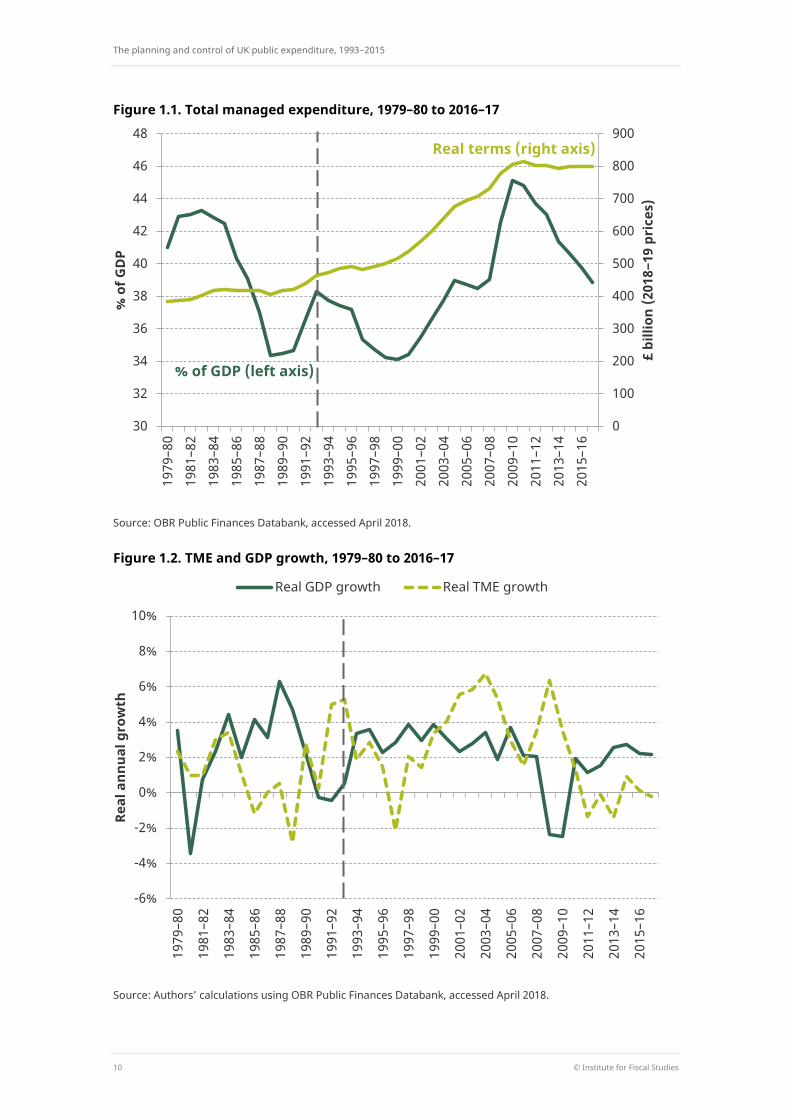
It is also important to remember that the level and direction of spending plans differed a lot between the periods. Figure 1.1 shows that public spending fell from 38.3% of GDP in 1992−93 to 34.1% in 1999−00. Spending then increased rapidly over the course of the 2000s, reaching 45.1% of GDP in 2009−10, partly due to the depressed level of GDP following the financial crisis. Spending then stayed flat in real terms after 2010 and fell sharply as a share of national income, dropping below 40% of GDP in 2015−16. The real growth rates in GDP and total managed expenditure (TME) are compared more explicitly in Figure 1.2, which shows how TME grew at a slower rate than GDP during the 1990s and 2010s. During the 2000s, spending grew at a faster rate than the wider economy – the difference was particularly stark in the 2000s following the financial crisis and associated economic downturn. This is relevant for our analysis to the extent that we might expect the system for the planning and control of spending to function somewhat differently during times of fiscal expansion from those of fiscal consolidation.
The composition of spending also changed over this time, as shown in Figures 1.3 and 1.4. In line with longer-term trends, spending on health continued to grow and account for an ever-increasing share of overall expenditure. Spending on overseas aid also increased substantially – albeit from a very low base. Social security spending on both pensioners and non-pensioners increased as a share of the total over this period, while spending on education and transport remained relatively stable. Spending on defence, debt interest and public order & safety accounted for smaller shares of public spending at the end of the period than at the start.2 Local authority expenditure stayed relatively constant over much of the period, accounting for slightly over a quarter of total spending between 1992−93 and 2009−10, before gradually falling to 22.5% of TME in 2015−16. The devolution of spending, and spending control, represented a major change over the period. This issue lies outside the scope of this report but will be addressed as part of the wider research project to which this report belongs.
2 For a more detailed discussion of changes to the composition of public spending over time, see S. Keynes and
G. Tetlow, ‘Survey of public spending in the UK’, Institute for Fiscal Studies, Briefing Note BN43, August 2014 (https://www.ifs.org.uk/publications/1791) and Institute for Fiscal Studies, ‘Fiscal facts’ (https://www.ifs.org.uk/tools_and_resources/fiscal_facts/public_spending_survey/composition_of_public_spending/).
The planning and control of UK public expenditure, 1993−2015
10 © Institute for Fiscal Studies
Figure 1.1. Total managed expenditure, 1979–80 to 2016–17
Source: OBR Public Finances Databank, accessed April 2018.
Figure 1.2. TME and GDP growth, 1979–80 to 2016–17
Source: Authors’ calculations using OBR Public Finances Databank, accessed April 2018.
0
100
200
300
400
500
600
700
800
900
30
32
34
36
38
40
42
44
46
48
1979
–80
1981
–82
1983
–84
1985
–86
1987
–88
1989
–90
1991
–92
1993
–94
1995
–96
1997
–98
1999
–00
2001
–02
2003
–04
2005
–06
2007
–08
2009
–10
2011
–12
2013
–14
2015
–16
£ bi
llion
(201
8−19
pri
ces)
% o
f GD
P
-6%
-4%
-2%
0%
2%
4%
6%
8%
10%
1979
–80
1981
–82
1983
–84
1985
–86
1987
–88
1989
–90
1991
–92
1993
–94
1995
–96
1997
–98
1999
–00
2001
–02
2003
–04
2005
–06
2007
–08
2009
–10
2011
–12
2013
–14
2015
–16
Real
ann
ual g
row
th
Real GDP growth Real TME growth
Real terms (right axis)
% of GDP (left axis)

Introduction
© Institute for Fiscal Studies 11
Figure 1.3. Public service spending, 1992–93 to 2015–16
Source: Authors’ calculations based on various Public Expenditure Statistical Analyses and OBR Public Finances Databank.
Figure 1.4. Public spending on social security and debt interest, 1992–93 to 2015–16
Source: Authors’ calculations based on various Public Expenditure Statistical Analyses, DWP Benefit Expenditure Tables 2017 and OBR Public Finances Databank.
0
2
4
6
8
10
12
14
16
18
20 19
92–9
3 19
93–9
4 19
94–9
5 19
95–9
6 19
96–9
7 19
97–9
8 19
98–9
9 19
99–0
0 20
00–0
1 20
01–0
2 20
02–0
3 20
03–0
4 20
04–0
5 20
05–0
6 20
06–0
7 20
07–0
8 20
08–0
9 20
09–1
0 20
10–1
1 20
11–1
2 20
12–1
3 20
13–1
4 20
14–1
5 20
15–1
6
% o
f tot
al m
anag
ed e
xpen
ditu
re
Health Public order & safety Education
Transport Defence Overseas aid
0
2
4
6
8
10
12
14
16
18
20
1992
–93
1993
–94
1994
–95
1995
–96
1996
–97
1997
–98
1998
–99
1999
–00
2000
–01
2001
–02
2002
–03
2003
–04
2004
–05
2005
–06
2006
–07
2007
–08
2008
–09
2009
–10
2010
–11
2011
–12
2012
–13
2013
–14
2014
–15
2015
–16
% o
f tot
al m
anag
ed e
xpen
ditu
re
Social security (pensioners) Social security (non-pensioners) Gross debt interest

The planning and control of UK public expenditure, 1993−2015
12 © Institute for Fiscal Studies
Our methodology In order to provide a quantitative assessment of the predictability of public spending over time, we compare successive spending plans with out-turns. We examine the match between plans and out-turns in each financial year to provide an indication of how effectively spending was controlled across periods, with particular focus on how the regime for planning and controlling public expenditure changed over time. This allows us to assess when spending differed from plans, and why. We examine headline spending figures, as well as more granular measures of public spending, such as the split between current and capital expenditure and spending by different departments.
Throughout our analysis, we need to be careful to compare like-with-like. Spending figures published today are rarely consistent with those published five years ago – never mind those published a quarter of a century ago. Changes in the statistical classification of spending items, the restructuring of government departments and changes to accounting methodology are just some of the reasons why a simple comparison between original spending plans and the most recent out-turns is likely to be misleading. To address this, we take out-turns from fiscal documents published shortly after the end of the financial year in question and make adjustments where appropriate. This approach, which we describe as using the ‘concurrent out-turn’, is explained in more detail in Appendix A.
Interpreting our results There are limitations to this approach. A deviation from plan may not necessarily be due to a lack of ‘control’. In reality, all deviations from plan are sanctioned by the Treasury. Often, rather than have spending deviate from plan, the plans are simply changed. There are times when there might be a ‘good’ reason to change plans, and the ability for a government to do so might be an example of the effective exertion of control. To take an extreme example, in the case of the outbreak of war or an epidemic, we would not want the government to be bound by its previous spending plans. In less dramatic times, we might think that an ‘overspend’ due to the government choosing to boost spending on priority areas if the economy performs better than expected is different from an ‘overspend’ due to a failure to keep departmental spending within pre-prescribed limits.
In addition to this, there are undoubtedly better and worse ways to meet plans. Lack of transparency in some aspects of the government accounts can make it difficult to see whether spending has turned out close to plan due to effective control on the part of the Treasury or due to some ‘gaming’ of the rules and figures. And there is also the question of whether an underspend relative to plan is as bad, or undesirable, as an overspend.
The rest of the report is structured chronologically as follows. Chapter 2 examines spending control between 1993−94 and 1998−99 under the ‘new control total’ regime. Chapter 3 covers the period under Labour between 1999−00 and 2009–10, following the introduction of the DEL/AME framework for the planning and control of spending. Chapter 4 then considers the period starting in 2010–11 under the Conservative–Liberal-Democrat coalition government. Chapter 5 concludes.
The new control total: 1993−94 to 1998−99
© Institute for Fiscal Studies 13
2. The new control total: 1993−94 to 1998−99
2.1 Introduction
The ‘new control total’ regime In the 1992 Autumn Statement, the government announced a new system for the planning and control of public expenditure under which an annual cash ceiling would be set in terms of a new control total (NCT). This followed the shock of the early 1990s recession and the UK’s ejection from the Exchange Rate Mechanism. The new process for controlling spending was thus introduced at a time of considerable reflection and more general change within HM Treasury.
The NCT represented around 85% of total public spending. The most cyclical components of public expenditure – namely, cyclical social security payments3 and interest payments on government debt – were excluded, along with proceeds from privatisation and various accounting adjustments. Everything else, including expenditure that local authorities financed themselves, was included. The definition of NCT was designed so that it would be broadly insulated from the effects of the economic cycle but would represent the majority of general government expenditure, which the government ultimately wished to control over time.
The ceiling for control total spending was set in advance in cash terms as part of an explicitly ‘top-down’ approach. Departments’ spending plans were set for the next three years, but years 2 and 3 were only indicative and could be revised at subsequent Budgets. There was extremely limited scope for unused cash to be carried forward from year to year. To allow some flexibility, each year’s planned control total included a reserve, which was not allocated to a department but was set aside for unforeseen spending requirements. This gave the government a margin within which to respond to unexpected events without breaching the overall spending ceiling. The reserve could either be allocated to a particular department in the second or third year of the planning period or be removed from spending plans altogether.
To understand the rationale for the introduction of the NCT framework, it is important to understand the government’s overarching fiscal objectives and the problems identified with the previous system.
The government’s fiscal objectives The new approach was designed to ensure that the government met its objective of reducing public spending as a share of national income over time.4 Total public spending was expressed in terms of general government expenditure (GGE) excluding privatisation
3 Cyclical social security payments were defined as unemployment benefit and income support for non-
pensioners. 4 This broad objective was in place from November 1992. From November 1995, the government was
committed to reducing public spending to below 40% of GDP. Sources: paragraph 2.01 of Autumn Statement November 1992 and paragraph 1.03 of Financial Statement and Budget Report 1996–97, November 1995.

The planning and control of UK public expenditure, 1993−2015
14 © Institute for Fiscal Studies
proceeds. Rather than seeking to control GGE directly, the government aimed to limit growth of total spending through control of the NCT.
The ceiling for the NCT was set in cash terms but was intended to reflect a maximum permitted real growth rate of 1.5% a year. That meant that growth in the NCT was to be ‘constrained to a rate which ensures that total public spending – general government expenditure – grows by less than the economy as a whole over the economic cycle’.5 This was consistent with assumptions about the trend rate of growth in spending on items outside the NCT but within GGE, and the maximum real growth rate was subject to review if those assumptions changed over time.
The previous framework The two main problems the architects of this system identified with the previous planning and control framework were the lack of distinction between cyclical and non-cyclical spending and the inability to take strategic decisions over the total level of public spending.
Cyclical spending The NCT was preceded by the planning total, the latest variant of which was introduced in July 1988. This ‘new planning total’ covered the spending that the central government was responsible for determining. The differences between the planning total and the new control total are summarised in Table 2.1.
Table 2.1. Relationship between planning total, NCT and GGE General government expenditure
of which: of which:
Planning total: New control total:
Social security: • non-cyclical • cyclical
Other programmes Privatisation proceeds Reserve
Social security: • non-cyclical
Other programmes LASFEa Reserve
Outside planning total: Outside new control total:
LASFEa Central government debt interest Accounting adjustments
Cyclical social security Central government debt interest Privatisation proceeds Accounting adjustments
a LASFE refers to local authority self-financed expenditure.
Source: Table 2.C.1 of Autumn Statement 1992.
5 Paragraph 2.02 of Autumn Statement November 1992.
The new control total: 1993−94 to 1998−99
© Institute for Fiscal Studies 15
Under the planning total, cyclical spending was not separated out from non-cyclical spending. There was a concern that in recession, the automatic rise in cyclical spending – on unemployment benefits, for instance – could squeeze other spending programmes, especially public investment. In recovery, falling cyclical spending could obscure rising discretionary spending within the total and make it more difficult to discern underlying trends. The NCT framework was a first attempt to distinguish between structural spending and more temporary spending driven by the business cycle.
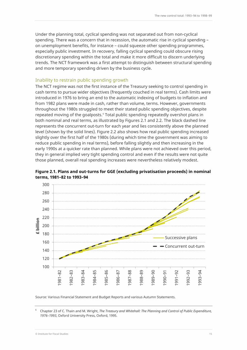
Inability to restrain public spending growth The NCT regime was not the first instance of the Treasury seeking to control spending in cash terms to pursue wider objectives (frequently couched in real terms). Cash limits were introduced in 1976 to bring an end to the automatic indexing of budgets to inflation and from 1982 plans were made in cash, rather than volume, terms. However, governments throughout the 1980s struggled to meet their stated public spending objectives, despite repeated moving of the goalposts.6 Total public spending repeatedly overshot plans in both nominal and real terms, as illustrated by Figures 2.1 and 2.2. The black dashed line represents the concurrent out-turn for each year and lies consistently above the planned level (shown by the solid lines). Figure 2.2 also shows how real public spending increased slightly over the first half of the 1980s (during which time the government was aiming to reduce public spending in real terms), before falling slightly and then increasing in the early 1990s at a quicker rate than planned. While plans were not achieved over this period, they in general implied very tight spending control and even if the results were not quite those planned, overall real spending increases were nevertheless relatively modest.
Figure 2.1. Plans and out-turns for GGE (excluding privatisation proceeds) in nominal terms, 1981–82 to 1993–94
Source: Various Financial Statement and Budget Reports and various Autumn Statements.
6 Chapter 23 of C. Thain and M. Wright, The Treasury and Whitehall: The Planning and Control of Public Expenditure,
1976–1993, Oxford University Press, Oxford, 1995.
100
120
140
160
180
200
220
240
260
280
300
1981
–82
1982
–83
1983
–84
1984
–85
1985
–86
1986
–87
1987
–88
1988
–89
1989
–90
1990
–91
1991
–92
1992
–93
1993
–94
£ bi
llion
Successive plans
Concurrent out-turn

The planning and control of UK public expenditure, 1993−2015
16 © Institute for Fiscal Studies
Figure 2.2. Plans and out-turns for GGE (excluding privatisation proceeds) in real terms, 1981–82 to 1993–94
Source: Authors’ calculations using various Financial Statement and Budget Reports, various Autumn Statements and March 2018 GDP deflators. Real spending expressed in 1993–94 prices.
In the 1980s and early 1990s, the aggregate level of public expenditure was decided through discussions in Cabinet and bilateral negotiations between the Treasury and departments. The overall level of spending therefore tended to emerge through compromises reached with spending ministers, rather than through a determination of what was ‘affordable’. Thain and Wright (1995) argue that the introduction of the NCT was an explicit admission of the past failure of the previous system, where Chief Secretaries repeatedly failed to deliver a planned total for the aggregate of public expenditure agreed by the Chief Secretary and Cabinet earlier in the year.7 So, while the Treasury may have targeted a particular level of aggregate spending throughout its discussions with departments, the process did not begin with a fixed overall ‘spending envelope’. The new explicitly top-down approach under the NCT regime was intended to make it easier to take strategic decisions relating to aggregate public expenditure before engaging in bilateral discussions with departments. Indeed, the ceiling was to be ‘based on what the nation can afford – not upon what spending departments would like to spend in an ideal world’.8 This new approach, it was hoped, would in turn make it easier to limit the growth of public spending and reduce it as a share of national income over time.
7 Chapter 23 of C. Thain and M. Wright, The Treasury and Whitehall: The Planning and Control of Public Expenditure,
1976–1993, Oxford University Press, Oxford, 1995. 8 Kenneth Clarke MP, Mansion House speech, 15 June 1993.
100
120
140
160
180
200
220
240
260
280
300
1981
–82
1982
–83
1983
–84
1984
–85
1985
–86
1986
–87
1987
–88
1988
–89
1989
–90
1990
–91
1991
–92
1992
–93
1993
–94
Rea
l £ b
illio
n (1
993−
94 p
rice
s)
Successive plans
Concurrent out-turn
The new control total: 1993−94 to 1998−99
© Institute for Fiscal Studies 17
2.2 Controlling the control total
We now turn to an assessment of how effective the government was at controlling public spending over the period when the NCT regime was in place. In line with the approach outlined in the introduction, we do so by comparing spending plans with out-turns.
The period 1993−94 to 1998−99 was presided over by three Chancellors of the Exchequer. Norman Lamont presided over the introduction of the new control total, before being replaced by Kenneth Clarke in 1993. As discussed in the previous section, the broad fiscal objective of the Conservative government over this period was to reduce public spending as a share of national income. Gordon Brown became Chancellor after Labour’s successful 1997 election campaign, in which it promised to be ‘wise spenders, not big spenders’9 and to work within departmental ceilings for spending already announced by their predecessors in the November 1996 Budget.10 This included plans up to and including the financial year 1998−99.
Each Budget published spending plans for the following three financial years, along with an out-turn for the previous year and an estimated out-turn for the year in progress. The first unified Budget was published in November 1993, which combined both tax and spending decisions (bringing an end to the publication of tax plans in the spring and spending plans in the autumn).
Headline spending Figure 2.3 shows plans and out-turns for headline control total spending and tells us a number of things.
First, plans were repeatedly revised down in cash terms. For instance, the cash ceiling for 1996−97 was revised down from £272.3 billion in the November 1993 Budget, to £263.5 billion in the November 1994 Budget, to £260.2 billion in the November 1995 Budget.
Second, despite these repeated downward revisions, spending consistently turned out lower than planned.11 That is, the black dashed line (indicating the concurrent out-turn series) lies below the solid lines showing successive NCT plans. This is in stark contrast to Figure 2.1 (which shows plans and out-turns for total spending, rather than the government’s planned total), in which spending repeatedly turned out above plans. Note also that Labour successfully stayed within the cash ceilings for 1997−98 and 1998−99 set out by Kenneth Clarke in his November 1996 Budget.
Real growth Recall that the NCT was set in cash terms so as to limit average real growth to a maximum of 1.5% per annum. Figure 2.4 shows annual real growth in the new control total from 1986−87 onwards.12 The NCT was not targeted by the government until 1993−94 but growth rates for previous years are provided for context.
9 Labour Party, New Labour, New Life for Britain, July 1996. 10 Chief Secretary to the Treasury, Alistair Darling MP, HM Treasury Press Release 89/97, 24 July 1997. 11 This result is robust to alternative choices of out-turn series. 12 Note that data limitations prevent us from including growth rates for years prior to 1986−87.

The planning and control of UK public expenditure, 1993−2015
18 © Institute for Fiscal Studies
Figure 2.3. Control total plans and out-turns, 1992–93 to 1998–99
Source: Various Financial Statement and Budget Reports (FSBRs) and various Public Expenditure Statistical Analyses.
Figure 2.4. Real growth in NCT spending, 1986–87 to 1998–99
Source: Authors’ calculations using various Public Expenditure Statistical Analyses and March 2018 GDP deflators. Growth rates are calculated using consistent spending series.
220
230
240
250
260
270
280
1992–93 1993–94 1994–95 1995–96 1996–97 1997–98 1998–99
£ bi
llion
November 1992 FSBR
November 1993 FSBR
November 1994 FSBR
November 1995 FSBR
November 1996 FSBR
Concurrent out-turn
-2%
-1%
0%
1%
2%
3%
4%
5%
6%
7%
1986
–87
1987
–88
1988
–89
1989
–90
1990
–91
1991
–92
1992
–93
1993
–94
1994
–95
1995
–96
1996
–97
1997
–98
1998
–99
Real
% c
hang
e
Pre NCT introduction
Post NCT introduction

The new control total: 1993−94 to 1998−99
© Institute for Fiscal Studies 19
It can be seen that real growth in the NCT slowed from 1993−94, the first financial year in which expenditure was measured in those terms for control purposes. While real growth did exceed 1.5% in some years, the average annual growth rate between 1992−93 and 1998−99 was 0.8%, comfortably below the government’s self-imposed limit.13 This, combined with the persistent undershooting of cash plans, could be interpreted as indicative of a high degree of spending control.
The picture is muddied, however, when we consider how these real growth rates compared with those implied by the government’s spending plans. Real spending can differ from plans due to a change in cash spending or because inflation turned out different from forecast. The official benchmark for inflation during the period was the Retail Prices Index (RPI) excluding mortgage interest payments, or RPIX, which would be a key determinant of the growth in some areas of spending – notably social security. When making forecasts of spending growth in real terms, however, the relevant measure is the change in the GDP deflator. If, in a given year, cash spending turned out exactly to plan, but growth in the GDP deflator was higher than expected, the real growth rate would be lower than planned. The opposite would be true if the GDP deflator grew by less than expected.
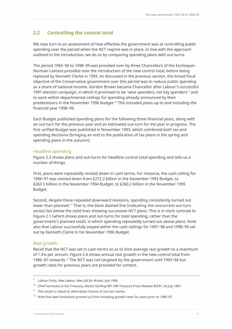
We are able to disentangle the differences from planned real growth due to differences in spending levels from the differences due to inflation forecast errors. The results are shown in Figure 2.5. The left-hand (dark green) bars show the planned real growth rates: those implied by the nominal spending plans and GDP deflator forecasts in the previous year’s Budget (e.g. the 1994−95 plans are taken from the November 1993 Budget). The middle bars show the real growth that would have resulted had nominal spending turned out exactly in line with those plans (calculated using out-turn inflation data). The right-hand (light green) bars show the out-turn real growth rate, as in Figure 2.4.
Real spending cuts were planned, but not achieved, in 1994−95 and 1995−96. This was due in large part to lower-than-expected inflation. Spending also grew by more than planned in nominal terms because in-year estimated spending – against which the planned real growth rate was calculated – tended to be revised downwards, which pushes up the out-turn growth rate in the out-turn data. In 1996−97, cash plans were broadly stuck to, and inflation turned out higher than expected, allowing the government to make a pronounced real reduction in control total spending. Perhaps the lesson here is that achieving real spending objectives requires not just tight control of nominal spending, but also inflation to turn out as expected.
To summarise, over the period as a whole, the government succeeded in staying within the cash ceilings set for the NCT. Lower-than-forecast inflation made this task easier, but led to real growth overshooting plans in some years, and meant that spending only fell in real terms in 1996−97. Nonetheless, average real growth in the NCT was successfully kept comfortably below the maximum rate the government had set itself, and this over a period when plans were tight and spending did, as planned, fall as a fraction of national income.
13 Real growth rates have been calculated here using March 2018 GDP deflators, in line with similar calculations
throughout this report. Using July 2000 GDP deflators produces slightly different figures and implies a lower average real growth rate between 1993−94 and 1998−99 (0.2% rather than 0.8%).
The planning and control of UK public expenditure, 1993−2015
20 © Institute for Fiscal Studies
Figure 2.5. Planned and out-turn real change in control total spending, 1993–94 to 1998–99
Source: Authors’ calculations using various Autumn Statements, various Financial Statement and Budget Reports, various Public Expenditure Statistical Analyses and March 2018 GDP deflators. Planned real growth in spending comes from the first year of spending plans in the previous FSBR compared with the in-year estimated out-turn.
2.3 Components of the NCT
Headline figures only give part of the story: to better understand why out-turns differed from plans, we also need to analyse what happened within the NCT. Even if total spending turned out as planned, this could obscure differential trends within that total and the possibility of underspends in some areas being used to offset overspends elsewhere.
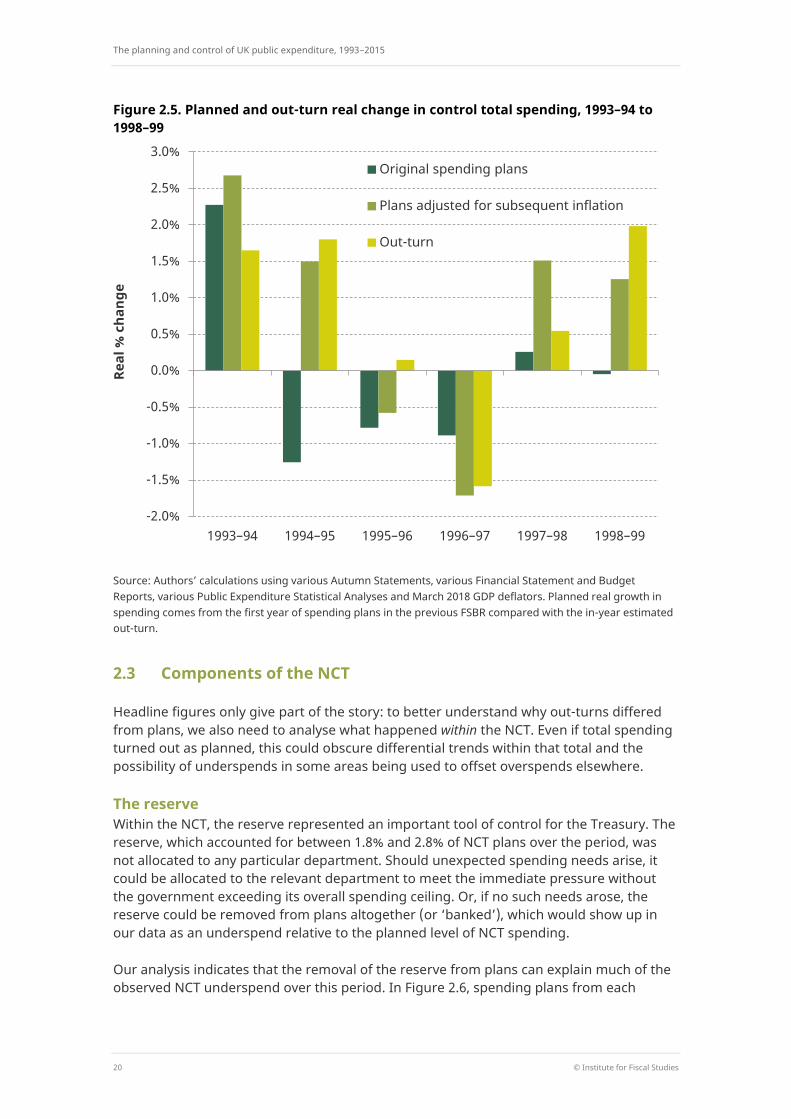
The reserve Within the NCT, the reserve represented an important tool of control for the Treasury. The reserve, which accounted for between 1.8% and 2.8% of NCT plans over the period, was not allocated to any particular department. Should unexpected spending needs arise, it could be allocated to the relevant department to meet the immediate pressure without the government exceeding its overall spending ceiling. Or, if no such needs arose, the reserve could be removed from plans altogether (or ‘banked’), which would show up in our data as an underspend relative to the planned level of NCT spending.
Our analysis indicates that the removal of the reserve from plans can explain much of the observed NCT underspend over this period. In Figure 2.6, spending plans from each
-2.0%
-1.5%
-1.0%
-0.5%
0.0%
0.5%
1.0%
1.5%
2.0%
2.5%
3.0%
1993–94 1994–95 1995–96 1996–97 1997–98 1998–99
Real
% c
hang
e
Original spending plans
Plans adjusted for subsequent inflation
Out-turn
The new control total: 1993−94 to 1998−99
© Institute for Fiscal Studies 21
Figure 2.6. NCT plans with and without reserve versus out-turns, 1992–93 to 1998–99
Source: Various Financial Statement and Budget Reports and various Public Expenditure Statistical Analyses.
November Budget are plotted with and without the reserve, along with the concurrent out-turn for NCT spending.
The solid green lines show the full NCT spending plans – these are identical to the plans shown in Figure 2.3. The dotted green lines show the same plans, but with the reserve removed for each year. The black dashed line, as in previous figures, shows the concurrent out-turn. For the most part, the out-turn lies above the dotted lines and below the solid lines. That is, spending turned out higher than if the reserve had been entirely removed from plans every year, but lower than if it had been entirely spent. This suggests that the reserve was partially, but not fully, allocated to spending programmes.
How we interpret this result for our assessment of control depends on a number of questions relating to the reserve, on which quantitative analysis can only take us so far.
The first relates to how the Chancellor and the Treasury thought of the reserve. Examining the data cannot tell us whether the reserve was intended to act as a ‘buffer’, so that the government could overspend in some areas without exceeding the overall cash ceiling. Or the government may always have intended to spend it, but at the point plans were set it did not yet know where.
There is also a question over exactly what type of unforeseen spending requirement the reserve was intended for. For instance, measures to combat the outbreak of bovine spongiform encephalopathy (BSE), commonly known as mad cow disease, placed
220
230
240
250
260
270
280
1992–93 1993–94 1994–95 1995–96 1996–97 1997–98 1998–99
£ bi
llion
Successive plans with Reserve
Successive plans without Reserve
Concurrent out-turn

The planning and control of UK public expenditure, 1993−2015
22 © Institute for Fiscal Studies
considerable demand on the reserve towards the end of the period, to the tune of £1.5 billion in 1996−97.14 Other allocations from the reserve were arguably made in response to political pressure rather than genuinely unforeseen events that necessitated an increase in public spending.15 For instance, in the same Budget as the £1.5 billion allocation was made from the reserve to combat BSE, Kenneth Clarke used the reserve to increase spending on the NHS, schools, police and prisons.16 In July 1997, Gordon Brown announced that £1.2 billion from the 1998–99 reserve would be allocated to the NHS and £1 billion to the education budget.17 Retaining the ability to allocate additional funds to priority areas in response to political pressure without breaching overall spending ceilings (even if the government always planned to spend more on those areas) could be interpreted as effective control of spending. But it might change how we think of the role of the reserve.
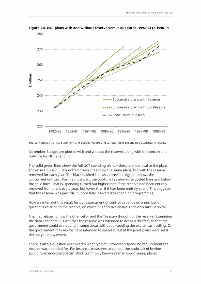
Finally, the inclusion of a relatively large reserve within spending plans arguably was indicative of the priority the Treasury placed on controlling total spending rather than its components. When a larger share of the planned total is unallocated, that makes it more difficult to assess the intended pattern of spending on particular spending programmes, as they could be topped up later from the reserve. Figure 2.7 shows the extent to which this was the case. While a larger reserve makes it easier to stay within a given cash ceiling, this can come at a cost: namely, the lack of stable, predictable departmental funding paths. Interestingly, the size of the reserve fell over this period18 − perhaps in response to the fact that significant amounts were removed from plans in 1993−94 and 1994−95.
Differences from departmental spending plans As well as an overall spending envelope, each Budget published departmental spending plans for the next three years. We are able to compare these plans to out-turn spending to estimate the extent of underspending or overspending by each department. This in turn is related to the reserve. An overspend relative to plan indicates that money from the reserve was allocated to the department in question. This could be offset by an underspend elsewhere. Priority was given to controlling the total, rather than its components, but this analysis gives an indication of which areas the Treasury found more difficult to control, which in turn is useful for understanding subsequent decisions relating to the boundary of the control total.
Figure 2.7 summarises differences from departmental spending plans over the NCT period along with estimated net allocations from the reserve. The horizontal black lines show the full reserve in each year; this varied from £4.0 billion in 1993−94 to £2.5 billion in 1996−97 and 1997−98. The black crosses show the net amount allocated from the reserve in each year. The difference between these points represents the underspend in the control total. For instance, spending turned out £3.0 billion below plan in 1993−94, suggesting that £1.0 billion of the £4.0 billion reserve was spent. In 1995−96 and 1996−97, NCT spending turned out around £0.4 billion lower than planned. This indicates that most of the reserve
14 Paragraph 4.22 of Financial Statement and Budget Report November 1996. 15 The best example of such an event in this period is the BSE crisis, but the classic example is the spending
associated with an unexpected war. 16 Paragraph 5.16 of Financial Statement and Budget Report November 1996. 17 Chancellor of the Exchequer, Gordon Brown MP, Budget Statement, 2 July 1997. 18 As part of wider spending plans, the reserve was set at each Budget for the next three financial years. The
average proportion of the NCT over the planning period accounted for by the reserve fell from 2.8% at the November 1992 Autumn Statement to 1.8% at the November 1996 Budget.
The new control total: 1993−94 to 1998−99
© Institute for Fiscal Studies 23
Figure 2.7. Differences from departmental plans, 1993–94 to 1998–99
Note: LASFE represents local authority self-financed expenditure.
Source: Authors’ calculations based on various Autumn Statements, Financial Statement and Budget Reports, and Public Expenditure Statistical Analyses.
was allocated to departments in each of those years. In 1997−98, control total spending turned out £3.6 billion lower than planned, with a reserve for the year of only £2.5 billion. This suggests that the amount of underspending by departments by far exceeded any overspending relative to department plans, which is why the black cross lies below zero.
Our analysis also allows us to see which departments overspent relative to initial plans, and therefore needed their spending ‘topped up’. This is shown for a number of departments in Figure 2.7 by the coloured bars. Overall, social security and LASFE appear to have been the spending domains showing the largest deviations from spending plans. This is perhaps not overly surprising: social security is more ‘demand-led’ than other areas of spending, even when non-cyclical. And LASFE, by definition, is determined by local authority decisions, over which the Treasury has no direct control.19
Public sector pay and running costs During this period, two key areas targeted for spending reductions were public sector pay and departmental running costs. In February 1993, the government announced that it
19 However, as noted in the 1992 Autumn Statement, the government was able to influence and restrain local
authority expenditure, and hence LASFE, through grant, capping and capital receipts rules. See paragraph 2C.9 of Autumn Statement November 1992.
-5
-4
-3
-2
-1
0
1
2
3
4
5
1993–94 1994–95 1995–96 1996–97 1997–98 1998–99
£ bi
llion
Health Defence Non-cyclical social security LASFE Other Dummy Full reserve Allocated from reserve
This gap represents the overall underspend in control total spending

The planning and control of UK public expenditure, 1993−2015
24 © Institute for Fiscal Studies
would conduct ‘Fundamental Expenditure Reviews’. These reviews were intended to examine spending programmes across every department of state to assess the sustainability of long-term trends and inform decisions taken by the Treasury on departments’ spending settlements. The November 1993 Budget noted that ‘Public sector pay and running costs were identified as key candidates for reductions: the greater the restraint on paybills the more resources available for service provision and capital spending’.20 To that end, running costs for central government departments were frozen at the 1993−94 level and any pay increases had to be offset, or more than offset, by efficiencies and other economies. Thus the cost of pay settlements had to be met within existing budgets. This approach was then reaffirmed through announcements from the Chancellor in September 1994, September 1995 and September 1996.
Data limitations prevent us from conducting a thorough quantitative analysis, and we are unable to compare plans with out-turns as we do elsewhere in this report. However, the available evidence does suggest that the government achieved its stated aims in this area. Gross expenditure on civil service departments’ running costs was broadly flat between 1993−94 and 1997−98, only rising from £13.1 billion to £13.2 billion in cash terms – a real-terms cut of more than 7%.21 Over the same period, the pay bill for civil servants and other staff covered by running costs fell from £8.4 billion to £7.8 billion, a reduction of more than 14% in real terms. Whilst we cannot assess whether these cuts were smaller or larger than those originally envisaged, it suggests that the government was successful in reducing real spending in these areas.
Figure 2.8. Difference between average public and private sector hourly pay, 1993 to 2015
Note: A positive difference means that public sector pay is higher than private sector pay, on average. Difference controlling for workers’ characteristics controls for differences in age, sex, education, experience and region.
Source: Authors’ calculations using Labour Force Survey 1993−2015.
20 Paragraph 5.30 of Financial Statement and Budget Report 1994−95, November 1993. 21 Authors’ calculations based on table 5.5 of Public Expenditure Statistical Analyses 1999−2000, March 1999.
0%
5%
10%
15%
20%
25%
30%
1993
19
94
1995
19
96
1997
19
98
1999
20
00
2001
20
02
2003
20
04
2005
20
06
2007
20
08
2009
20
10
2011
20
12
2013
20
14
2015
Aver
age
diff
eren
ce b
etw
een
publ
ic
and
priv
ate
sect
or h
ourl
y pa
y
Calendar year
Average difference Average difference after controlling for workers’ characteristics

The new control total: 1993−94 to 1998−99
© Institute for Fiscal Studies 25
We can, however, analyse how public sector pay fared compared with private sector pay over the period. Figure 2.8 plots the difference between public and private hourly pay between 1993 and 2015, showing both the raw average difference and the average difference after controlling for differences in workers’ characteristics. The figure shows that public sector pay is higher than private sector pay on average, but that this difference is smaller once we control for differences in workers’ characteristics.
We also observe that the average difference between public and private sector pay declined sharply during the NCT period. This trend continued into the early 2000s, before reversing after 2002 (though it never returned to the levels of the early 1990s). One interpretation of this is that the exertion of extremely ‘tight’ control of public sector pay in the short term stores up pressure for greater pay increases (and therefore higher spending) later. This argument could suggest that while the government’s extremely tight control over public sector pay in the short run helped to bring down spending, the extent of the reductions achieved in the 1990s could not be sustained.
2.4 Capital spending
In his Mansion House speech of October 1992, Norman Lamont acknowledged concerns that government spending plans did not adequately distinguish between current and capital spending.22 So, in order to ‘help to underpin the Government’s commitment to infrastructure investment in the longer run’, he announced that from the first unified Budget in November 1993, capital spending plans would be split out from wider spending. This was done at an aggregate level, rather than by department, and was expressed in terms of public sector capital expenditure.23
The separation of capital from current spending was not intended to lead to growing levels of capital investment, however. The November 1993 Budget noted that ‘Public sector capital spending was maintained at high levels during the recession. As the recovery continues, capital spending by the private sector is likely to rise and that in the public sector to fall. The overriding need for public spending to contribute towards the reduction in public borrowing means that capital spending will not be sustained at levels as high as in 1993−94’.24 That is, the government planned to cut capital spending over this period, reversing the increase that had occurred during the so-called Lawson boom.
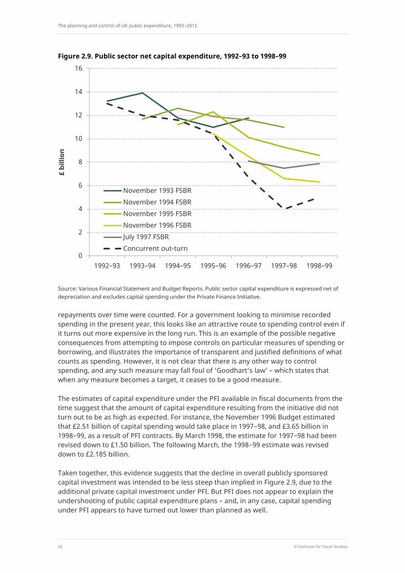
Figure 2.9 shows that plans for government capital spending were repeatedly revised downwards, and that capital spending fell even faster than planned, from around £13.0 billion in 1992−93 to £5.0 billion in 1998−99.
This definition of capital spending excludes capital spending under the Private Finance Initiative (PFI), which the government introduced and sought to expand over this period. Under the PFI, the public sector contracts to pay over a long period for services from a private sector provider, which is responsible for any capital investment required to undertake the project. This meant that up-front spending by the private provider on the capital investment was not counted against total government spending, though
22 Norman Lamont, Mansion House speech, 29 October 1992. 23 Note that throughout this section we express public sector capital expenditure net of depreciation. 24 Paragraph 5.19 of Financial Statement and Budget Report 1994−95, November 1993.
The planning and control of UK public expenditure, 1993−2015
26 © Institute for Fiscal Studies
Figure 2.9. Public sector net capital expenditure, 1992–93 to 1998–99
Source: Various Financial Statement and Budget Reports. Public sector capital expenditure is expressed net of depreciation and excludes capital spending under the Private Finance Initiative.
repayments over time were counted. For a government looking to minimise recorded spending in the present year, this looks like an attractive route to spending control even if it turns out more expensive in the long run. This is an example of the possible negative consequences from attempting to impose controls on particular measures of spending or borrowing, and illustrates the importance of transparent and justified definitions of what counts as spending. However, it is not clear that there is any other way to control spending, and any such measure may fall foul of ‘Goodhart’s law’ – which states that when any measure becomes a target, it ceases to be a good measure.
The estimates of capital expenditure under the PFI available in fiscal documents from the time suggest that the amount of capital expenditure resulting from the initiative did not turn out to be as high as expected. For instance, the November 1996 Budget estimated that £2.51 billion of capital spending would take place in 1997−98, and £3.65 billion in 1998−99, as a result of PFI contracts. By March 1998, the estimate for 1997−98 had been revised down to £1.50 billion. The following March, the 1998−99 estimate was revised down to £2.185 billion.
Taken together, this evidence suggests that the decline in overall publicly sponsored capital investment was intended to be less steep than implied in Figure 2.9, due to the additional private capital investment under PFI. But PFI does not appear to explain the undershooting of public capital expenditure plans – and, in any case, capital spending under PFI appears to have turned out lower than planned as well.
0
2
4
6
8
10
12
14
16
1992–93 1993–94 1994–95 1995–96 1996–97 1997–98 1998–99
£ bi
llion
November 1993 FSBR November 1994 FSBR November 1995 FSBR November 1996 FSBR July 1997 FSBR Concurrent out-turn
The new control total: 1993−94 to 1998−99
© Institute for Fiscal Studies 27
Figure 2.10. Public sector net investment as a share of GDP, 1985–86 to 2015–16
Source: Authors’ calculations based on OBR Public Finances Databank, accessed April 2018.
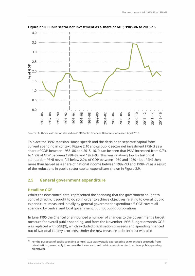
To place the 1992 Mansion House speech and the decision to separate capital from current spending in context, Figure 2.10 shows public sector net investment (PSNI) as a share of GDP between 1985−86 and 2015–16. It can be seen that PSNI increased from 0.7% to 1.9% of GDP between 1988−89 and 1992−93. This was relatively low by historical standards – PSNI never fell below 2.0% of GDP between 1950 and 1980 – but PSNI then more than halved as a share of national income between 1992−93 and 1998−99 as a result of the reductions in public sector capital expenditure shown in Figure 2.9.
2.5 General government expenditure
Headline GGE Whilst the new control total represented the spending that the government sought to control directly, it sought to do so in order to achieve objectives relating to overall public expenditure, measured initially by general government expenditure.25 GGE covers all spending by central and local government, but not public corporations.
In June 1995 the Chancellor announced a number of changes to the government’s target measure for overall public spending, and from the November 1995 Budget onwards GGE was replaced with GGE(X), which excluded privatisation proceeds and spending financed out of National Lottery proceeds. Under the new measure, debt interest was also
25 For the purposes of public spending control, GGE was typically expressed so as to exclude proceeds from
privatisation (presumably to remove the incentive to sell public assets in order to achieve public spending objectives).
0.0
0.5
1.0
1.5
2.0
2.5
3.0
3.5
4.0
1985
–86
1987
–88
1989
–90
1991
–92
1993
–94
1995
–96
1997
–98
1999
–00
2001
–02
2003
–04
2005
–06
2007
–08
2009
–10
2011
–12
2013
–14
2015
–16
% o
f GD
P

The planning and control of UK public expenditure, 1993−2015
28 © Institute for Fiscal Studies
measured net of the interest and dividends that the government receives from its assets, rather than on a gross basis. These differences meant that GGE(X) was consistently lower than GGE.26 The November 1995 Budget also announced that the government was aiming to reduce public expenditure to below 40% of GDP; expressing this target in terms of GGE(X) rather than GGE made it slightly easier to achieve this objective. In the event, spending measured by both GGE and GGE(X) fell below 40% of GDP in 1997−98,27 and the government was therefore successful in meeting its overall public spending objective.
Spending outside the control total General government expenditure included the entirety of the control total, plus cyclical social security, central government debt interest and a number of technical accounting adjustments. Following the election of Labour in 1997, some additional spending was also placed outside of the control total. This was spending relating to the ‘Welfare-to-Work’ programme and additional housing investment paid for through the phased release of local authority capital receipts. This amounted to an extra £0.4 billion of planned spending in 1997−98 and £1.9 billion in 1998−99. Neither of these spending programmes appeared particularly cyclical, and so the decision to place them outside of the control total does not appear to have been justified by economic reasons. This decision did, however, allow the government to increase spending on those areas without breaking the manifesto pledge to stay within the control total plans set in the November 1996 Budget. It is also important to note that ‘Welfare-to-Work’ was to be fully funded from the receipts of the one-off windfall tax on privatised utility companies.28
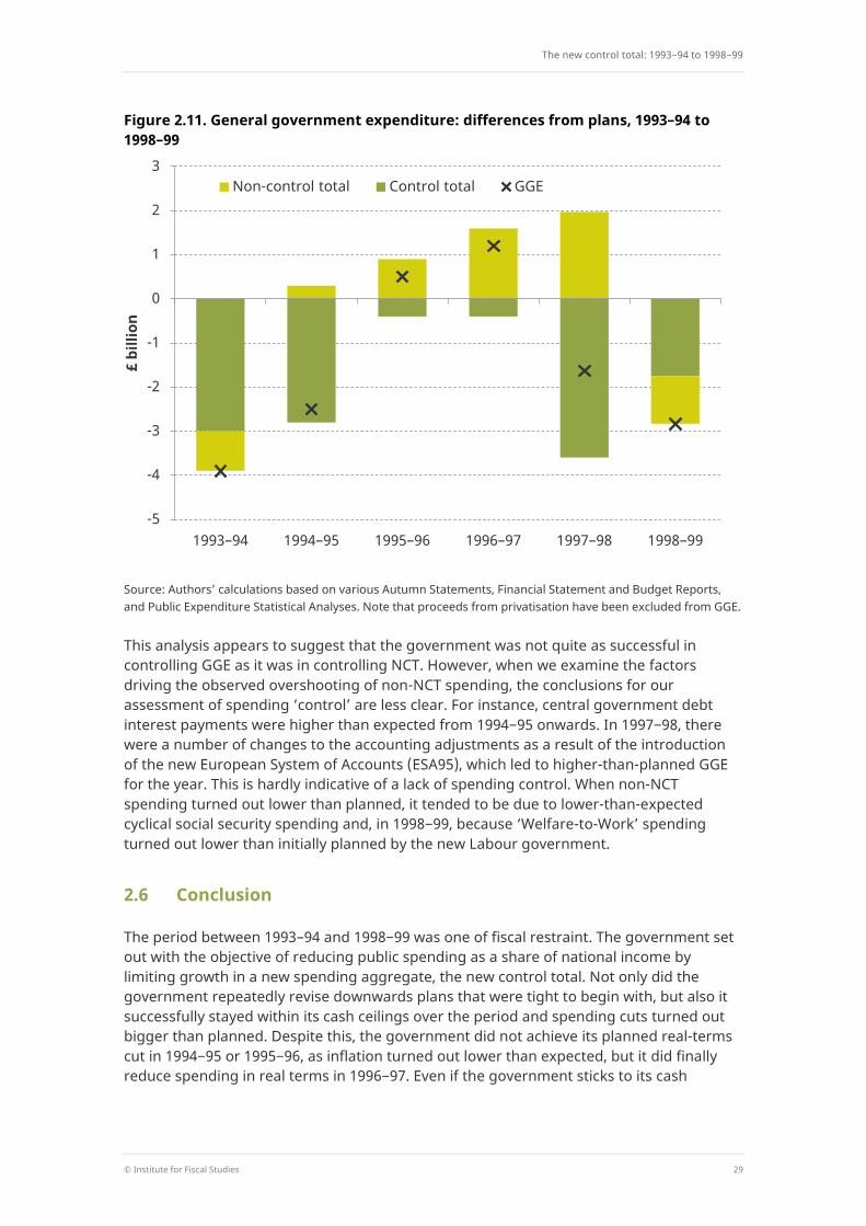
Differences from plans Figure 2.11 decomposes the differences from GGE29 plans set one year prior into control total and non-control total spending. The black crosses show the difference between out-turn general government expenditure and the planned level.30 In the first two and final two years of the period, GGE came in lower than planned. In 1995−96 and 1996−97, GGE exceeded the planned level.
The darker green bars show the difference in control total spending from the cash ceiling set out in the previous year’s Budget: these correspond to the underspends shown in earlier figures. The lighter green bars show deviation from plan that can be attributed to non-NCT elements of spending. In the first and final years, non-NCT spending (which includes cyclical social security and debt interest payments) was lower than planned; in the intervening years, it exceeded the planned level. In 1995−96 and 1996−97, this overspend was greater than the underspend in NCT spending and led to the overshooting of overall GGE plans.
26 Spending financed by the National Lottery amounted to around £0.5 billion in 1994–95; in the same year,
estimated interest payments net of receipts were £3.7 billion less than gross interest payments. Source: A. Dilnot and C. Giles (eds), Options for 1996: The Green Budget, Institute for Fiscal Studies, London, 2 October 1995.
27 As measured at the time – see table 4.1 of Public Expenditure Statistical Analyses 2000−01, April 2000. 28 Paragraph 3.24 of Financial Statement and Budget Report March 1998. 29 We use GGE excluding privatisation rather than GGE(X) in order to be able to analyse the whole period. 30 Note that because the Labour manifesto promised to stay within existing NCT plans from November 1996, but
made no reference to GGE, we here compare 1998−99 out-turns with the plans published in the July 1997 Budget.
The new control total: 1993−94 to 1998−99
© Institute for Fiscal Studies 29
Figure 2.11. General government expenditure: differences from plans, 1993–94 to 1998–99
Source: Authors’ calculations based on various Autumn Statements, Financial Statement and Budget Reports, and Public Expenditure Statistical Analyses. Note that proceeds from privatisation have been excluded from GGE.
This analysis appears to suggest that the government was not quite as successful in controlling GGE as it was in controlling NCT. However, when we examine the factors driving the observed overshooting of non-NCT spending, the conclusions for our assessment of spending ‘control’ are less clear. For instance, central government debt interest payments were higher than expected from 1994−95 onwards. In 1997−98, there were a number of changes to the accounting adjustments as a result of the introduction of the new European System of Accounts (ESA95), which led to higher-than-planned GGE for the year. This is hardly indicative of a lack of spending control. When non-NCT spending turned out lower than planned, it tended to be due to lower-than-expected cyclical social security spending and, in 1998−99, because ‘Welfare-to-Work’ spending turned out lower than initially planned by the new Labour government.
2.6 Conclusion
The period between 1993–94 and 1998−99 was one of fiscal restraint. The government set out with the objective of reducing public spending as a share of national income by limiting growth in a new spending aggregate, the new control total. Not only did the government repeatedly revise downwards plans that were tight to begin with, but also it successfully stayed within its cash ceilings over the period and spending cuts turned out bigger than planned. Despite this, the government did not achieve its planned real-terms cut in 1994−95 or 1995−96, as inflation turned out lower than expected, but it did finally reduce spending in real terms in 1996−97. Even if the government sticks to its cash
-5
-4
-3
-2
-1
0
1
2
3
1993–94 1994–95 1995–96 1996–97 1997–98 1998–99
£ bi
llion
Non-control total Control total GGE
The planning and control of UK public expenditure, 1993−2015
30 © Institute for Fiscal Studies
spending plans, achieving real-terms spending reductions also relies on inflation turning out as expected.
Total public expenditure (measured by GGE) occasionally exceeded the planned level, but it fell as a share of national income, dipping below the 40% target in 1997−98. This task was made easier by the favourable macroeconomic conditions, with the UK enjoying steady growth and economic recovery following its ejection from the European Exchange Rate Mechanism in September 1992. Upon entering government, Gordon Brown successfully stuck to the letter of Labour’s election pledge to stay within the cash ceilings for 1997−98 and 1998−99 announced by Kenneth Clarke in his November 1996 Budget – although this relied on Welfare-to-Work spending being placed outside of the control total.31
The persistent undershooting of plans was partly the result of not spending the full reserve in most years and partly came from departmental underspending. Tight control of departmental running costs and public sector pay also contributed to spending reductions. Within the NCT, social security and local authority self-financed expenditure appear to have deviated most notably from plans, with LASFE in particular persistently turning out higher than planned, somewhat offsetting underspends elsewhere. In 1998−99, the final year of our period, health spending received a substantial top-up from the reserve.
The nature of the planning framework in this period meant that the only plan that really mattered was the one made one year in advance: the second and third years of plans could be, and always were, changed. For this reason, the majority of our analysis in this chapter has focused on how spending turned out relative to the plans set in the previous year, but if out-turns are compared with plans set two and three years prior, the observed underspends are markedly larger. There is a question as to whether this impeded departments’ ability to plan, as budgets beyond the next financial year were always subject to change.
There is also the issue of whether spending turning out lower than planned is always an indication of control. This point is particularly salient when thinking about capital spending. The government paid lip service to its commitment to infrastructure investment, yet capital expenditure fell even faster than planned to historically low levels. The Conservative government introduced the Private Finance Initiative, presumably in part to take the place of public investment, but the available evidence suggests that much of the expected capital investment under PFI arrangements failed to materialise, even though it grew rapidly from a low base. It is fair to conclude that control of capital spending over this period was ineffective, and it could certainly be argued that consistent underspends were economically damaging. On the other hand, because new control totals were set as cash limits, as opposed to spending targets, it is unclear whether underspends in the overall NCT indicate a lack of control.
31 Interestingly, Clarke notes that ‘Gordon [Brown] fought, for public purposes at least, to adhere absolutely to
my figures with no flexibility at all. I on the other hand had always proceeded on the basis that I would have an annual spending round involving debates with my Cabinet colleagues in which I would be able to switch spending from one department to another in line with unexpected events, without threatening the overall figure’. See page 431 of K. Clarke, Kind of Blue: A Political Memoir, Macmillan, London, 2016.

The new control total: 1993−94 to 1998−99
© Institute for Fiscal Studies 31
Finally, whilst the government was successful in its fiscal consolidation, the sustainability of this level of ‘control’ over spending is questionable. Sustained cuts to capital spending, falling public sector pay and underinvestment in schools and hospitals likely stored up problems that required high public spending later. Exerting extremely tight ‘control’ to reduce spending in the short run could lead to the building up of pressures that push spending up in the longer run unless the control is accompanied by long-term plans to ensure sustainability.

The planning and control of UK public expenditure, 1993−2015
32 © Institute for Fiscal Studies
3. The DEL/AME regime under Labour: 1999−00 to 2009−10
3.1 Introduction
The Economic and Fiscal Strategy Report published in June 1998 announced a new regime for the planning and control of UK public spending to replace the NCT regime.32 Under the new framework, spending was to be split between departmental expenditure limits (DELs) and annually managed expenditure (AME). DELs were intended to cover spending that can be controlled, rather than being driven by demand or the economic cycle. The remainder of spending – that which the government argued could not reasonably be subject to firm multi-year limits – was classified as AME and was not subject to multi-year plans. Both initially represented roughly half of total managed expenditure (TME), which replaced general government expenditure as the measure of total public spending.
The DEL, AME and TME regime was accompanied by a set of fiscal rules which clearly distinguished current spending from capital spending. In particular, the aim for budget balance ‘over the cycle’ referred only to balancing revenues against current spending. Capital spending was not counted against this fiscal rule. It was to be constrained by the sustainable investment rule, which stated that government debt should not exceed 40% of national income.
Shortcomings of the NCT regime The new framework included a number of other innovations and was introduced in response to a number of issues identified with the pre-existing system.33
Short planning horizons Under the NCT regime, and since the early 1960s, the government operated a regime of annual Public Expenditure Surveys. Whilst plans were set for the next three years, the second and third years of plans were merely indicative, as plans were revisited and revised every year. Labour argued that this created an uncertain environment that hindered efforts by departments to plan their spending.
Underinvestment in capital The new government argued that the lack of distinction between current and capital spending under the previous system led to persistent underinvestment. Pointing to the historically low levels of capital spending (as measured by public sector net investment), it argued that when departmental budgets were cut back, it was easier to cut back on investment than on day-to-day spending, as the effects of those spending cuts would take longer to become apparent. For instance, underinvestment in roads, schools and hospitals might show up years later in the form of a build-up of maintenance backlogs, but the pain of cutting public sector pay would be felt immediately.
32 Economic and Fiscal Strategy Report June 1998. 33 HM Treasury, Planning Sustainable Public Spending: Lessons from Previous Policy Experience, London, November
2000.
The DEL/AME regime under Labour: 1999−00 to 2009−10
© Institute for Fiscal Studies 33
Strict annuality in budgeting If departments failed to spend their entire allocation, there was very limited scope for them to carry forward those unused resources to future years. This created incentives for departments to spend their remaining budget in the final months of the year, however wastefully. This so-called ‘use it or lose it’ mentality was thought to lead to poor value for money for the taxpayer.
Features of the new system To address the perceived issues with the planning and control of public expenditure, as well as distinguishing between DELs and AME, the new system was designed with the following features.
Fiscal rules Spending plans were made in the context of a wider fiscal policy and were set to ensure adherence to two fiscal rules:
1. The golden rule: over the economic cycle, the government will borrow only to invest and not to fund current spending.
2. The sustainable investment rule: the ratio of net public sector debt to GDP will be kept below a ‘stable and prudent’ level, interpreted as 40% of GDP.
These made a clear distinction between capital and current spending. The golden rule was explicitly intended to ensure that capital spending was not cut to reach overall budget balance and to ensure that both the Treasury and spending departments would treat capital and current spending quite differently.
Following the financial crisis and subsequent deterioration in the public finances, the existing fiscal rules were suspended. A ‘temporary operating rule’ was adopted in 2008, committing the government to ‘set policies to improve the cyclically-adjusted current budget each year, once the economy emerges from the downturn, so it reaches balance and debt is falling as a proportion of GDP once the global shocks have worked their way through the economy in full’.34 This was briefly replaced in 2010 by the Fiscal Responsibility Act (which legislated a particular reduction in borrowing by 2013–14) – but this was repealed by the new coalition government after the 2010 election (as described in more detail in Chapter 4).
Multi-year spending plans The government was to set ‘firm and realistic multi-year limits for departments’ expenditure’35 to cover a three-year period. The limits were set in cash terms to give departments an incentive to control their own costs, and the government planned for the limits to be reviewed only in the event of inflation varying substantially from forecast. The reserve was retained, but was intended to be small and used only for emergencies and genuine contingencies: departments would not be able to bid for extra funds each year, as they had in the past. Equally, the Treasury would not able to make incremental cuts at each annual spending round. Guaranteeing departments’ level of funding for the next
34 Paragraph 1.12 of HM Treasury, The Government’s Fiscal Framework, November 2008
(http://news.bbc.co.uk/1/shared/bsp/hi/pdfs/24_11_08_pbr_fiscalframework.pdf). 35 Economic and Fiscal Strategy Report June 1998.
The planning and control of UK public expenditure, 1993−2015
34 © Institute for Fiscal Studies
three years (rather than just one) would, it was hoped, give departments a solid base for planning operations on a sensible timescale.
Distinction between current and capital spending Within the overall spending aggregate of total managed expenditure, which covered all spending by the public sector, current and capital budgets were planned and managed separately. This was intended to address the perceived bias against capital investment and prevent investment spending from being cut back to meet short-term pressures on current expenditure. Departments were unable to use capital budgets to fund day-to-day spending.36
An expansion of end-year flexibility arrangements The Treasury had first introduced an end-year flexibility (EYF) scheme in July 1983, which allowed central government departments to carry forward a limited amount of underspending on capital programmes from year to year. This was gradually expanded to cover some other aspects of public spending, with special arrangements for the Ministry of Defence in particular, but was far from comprehensive.37 The new DEL/AME framework explicitly allowed for departments to carry forward 100% of unspent resources into the following financial year to combat the incentive for departments to engage in wasteful spending at year-end.
Spending outside of DEL remained subject to annual reviews Spending that the government argued could not reasonably be subject to firm multi-year plans was to be known as annually managed expenditure, or AME. AME included all social security spending, local authority self-financed expenditure (LASFE), debt interest payments, and net payments to EU institutions. It was not capped but was to be subject to annual scrutiny as part of the Budget process. The government argued that placing this more volatile expenditure outside of the three-year DEL totals would mean that sensible departmental planning would not be adversely affected by short-term fluctuations resulting from the business cycle. In many ways, this was a development of the ideas underlying the creation of the NCT.
The end of the unified Budget The government moved away from having a single fiscal event in the autumn of each year, instead choosing to publish a Budget in the spring and a Pre-Budget Report towards the end of the calendar year. This ultimately provided the Chancellor with two opportunities each year to make tax and spending decisions.
Resource accounting and budgeting In 1996, the government announced that it was going to change from cash-based budgeting to resource accounting and budgeting (RAB). The shift from cash-based plans to RAB did not all happen in one go. Spending Review 2000 was the first to be conducted on an ‘accruals’ basis, where rather than recording spending as having occurred when the cash went in or out (as under cash-based accounting), costs and revenues were ‘matched’
36 Funds earmarked for capital spending could be channelled into current expenditure only within an agreed
margin, which was set to allow for some managerial flexibility and for the financing of public–private partnerships.
37 Chapter 19 of C. Thain and M. Wright, The Treasury and Whitehall: The Planning and Control of Public Expenditure, 1976–1993, Oxford University Press, Oxford, 1995.
The DEL/AME regime under Labour: 1999−00 to 2009−10
© Institute for Fiscal Studies 35
to the period in which the activity relating to those costs or revenues occurred. From Spending Review 2002, non-cash costs were also incorporated into spending plans. This included ‘cost of capital’ charges and depreciation.
The move to RAB was intended to allow the government to better capture the full costs of resources consumed in delivering public services and improve the efficiency of public spending. Under a cash-based approach, once an asset had been bought, there were no further costs to the department (as no more cash would need to leave the door). This meant that departments had no incentive to dispose of under-utilised assets – despite the fact that there were opportunity costs of retaining them. Under a RAB approach, the accounts would give a more accurate representation of the true economic costs of delivering objectives and would make departments more aware of the true resource cost of holding capital.
It is interesting to note that while under RAB departments manage budgets that include non-cash costs, the main fiscal aggregates with which the Treasury is concerned for meeting the government’s fiscal rules (namely, cyclically-adjusted borrowing) do not take non-cash costs or financial transactions into account. This means that while departments are faced with the true economic costs of delivering objectives, the same may not be true of the Treasury if its focus is only on meeting the fiscal rules.
From its introduction, DEL was split into current and capital budgets. Following the introduction of RAB, these became resource (RDEL) and capital (CDEL). Depreciation and cost-of-capital charges were included in the resource budget; the capital budget included only spending that created new assets on the government’s balance sheet.
There are two further points relating to RAB that are relevant for our analysis. First, the shift to RAB means that pre-RAB figures are not consistent with those published later, complicating any comparison of plans with out-turns. Second, the planned introduction of RAB in 2000 meant that while Spending Review 1998 set out three years of departmental spending plans, the plans were always planned to be updated after two years (in 2000) when the government moved to RAB.38 We will return to this point later.
The Clear Line of Sight (Alignment) Project In July 2007, the government announced that it would be simplifying the presentation and publication of public expenditure data. Historically, the presentation of spending figures varied between plans (in Budgets or Spending Reviews), estimates (which were presented to parliament for approval), and resource accounts published at year-end. The Clear Line of Sight Project, or Alignment Project, was announced in response to criticism of this state of affairs.39 By reporting in a more consistent fashion at all three stages in the process, the reforms were intended to make it easier for users of the reports (and, in particular, parliament) to understand how resources have been used and to hold the government to account. The main change to the budgeting framework (the area most relevant for our analysis) was the removal of the near-cash/non-cash boundary from resource budgets (as this distinction does not exist within resource accounting) and the transfer of some non-
38 Economic and Fiscal Strategy Report June 1998. 39 Pages 35–36 of The Governance of Britain, Green Paper (Cm 7170), July 2007
(https://assets.publishing.service.gov.uk/government/uploads/system/uploads/attachment_data/file/228834/7170.pdf).
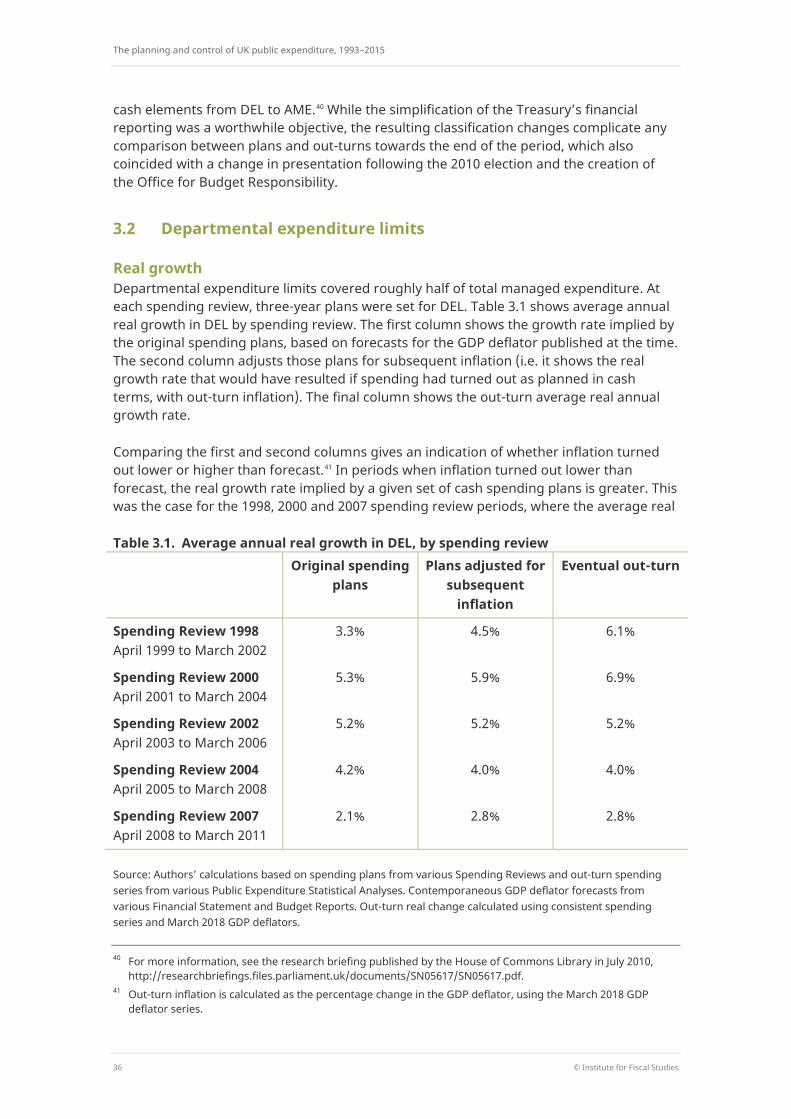
The planning and control of UK public expenditure, 1993−2015
36 © Institute for Fiscal Studies
cash elements from DEL to AME.40 While the simplification of the Treasury’s financial reporting was a worthwhile objective, the resulting classification changes complicate any comparison between plans and out-turns towards the end of the period, which also coincided with a change in presentation following the 2010 election and the creation of the Office for Budget Responsibility.
3.2 Departmental expenditure limits
Real growth Departmental expenditure limits covered roughly half of total managed expenditure. At each spending review, three-year plans were set for DEL. Table 3.1 shows average annual real growth in DEL by spending review. The first column shows the growth rate implied by the original spending plans, based on forecasts for the GDP deflator published at the time. The second column adjusts those plans for subsequent inflation (i.e. it shows the real growth rate that would have resulted if spending had turned out as planned in cash terms, with out-turn inflation). The final column shows the out-turn average real annual growth rate.
Comparing the first and second columns gives an indication of whether inflation turned out lower or higher than forecast.41 In periods when inflation turned out lower than forecast, the real growth rate implied by a given set of cash spending plans is greater. This was the case for the 1998, 2000 and 2007 spending review periods, where the average real
Table 3.1. Average annual real growth in DEL, by spending review Original spending
plans Plans adjusted for
subsequent inflation
Eventual out-turn
Spending Review 1998 April 1999 to March 2002
3.3% 4.5% 6.1%
Spending Review 2000 April 2001 to March 2004
5.3% 5.9% 6.9%
Spending Review 2002 April 2003 to March 2006
5.2% 5.2% 5.2%
Spending Review 2004 April 2005 to March 2008
4.2% 4.0% 4.0%
Spending Review 2007 April 2008 to March 2011
2.1% 2.8% 2.8%
Source: Authors’ calculations based on spending plans from various Spending Reviews and out-turn spending series from various Public Expenditure Statistical Analyses. Contemporaneous GDP deflator forecasts from various Financial Statement and Budget Reports. Out-turn real change calculated using consistent spending series and March 2018 GDP deflators.
40 For more information, see the research briefing published by the House of Commons Library in July 2010,
http://researchbriefings.files.parliament.uk/documents/SN05617/SN05617.pdf. 41 Out-turn inflation is calculated as the percentage change in the GDP deflator, using the March 2018 GDP
deflator series.
The DEL/AME regime under Labour: 1999−00 to 2009−10
© Institute for Fiscal Studies 37
growth rate implied by plans adjusted for subsequent inflation (the second column) exceeds the original spending plans (the first column). In the 2002 and 2004 spending reviews, inflation turned out roughly as forecast.
More interesting is how spending turned out given the inflation out-turn, which we can assess by comparing the second and third columns in Table 3.1. In the three-year period covered by Spending Review 1998, DEL increased at an average rate of 6.1% per year, relative to a planned rate (adjusted for inflation) of 4.5%. The picture for Spending Review 2000 looks very similar: DEL grew by 6.9% per year, exceeding the (adjusted) planned rate of 5.9%. In both cases, the discrepancy between the out-turn growth rate and the original planned growth rate was even greater.
The story from 2002 onwards is different. In the 2002 and 2004 spending reviews, inflation turned out broadly as forecast, and DEL spending grew in line with plans. In Spending Review (SR) 2007, inflation turned out lower than forecast, but spending grew in line with the plans adjusted for the inflation out-turn. This, at first glance, indicates that the government did a much better job of controlling spending within DEL in the second half of the period than the first.
Timing of deviations When we look more closely at what was driving the higher-than-planned real growth in SR 1998 and SR 2000, the picture is more nuanced. The planning periods overlapped: plans were set for three years, but rolled forward after only two. SR 1998 set out plans up to and including 2001−02. In the SR of July 2000, plans were rolled forward for another three years, starting from 2001−02, with spending for that year at a higher level than initially planned in SR 1998. A very similar thing happened at SR 2000: spending plans for 2003−04 were rolled forward at the July 2002 SR, increasing the planned level of spending for the year. This meant that spending grew by more than originally planned.
This faster-than-expected real growth did not purely come about as a result of overlapping plans, however: spending was also ‘topped up’ between spending reviews. For example, Budget 2000 allocated an additional £3 billion of current spending and £1 billion of capital spending within DEL for 2000−01.42 Budget 2002 added an additional £4 billion to DEL for 2003−04.43 These additions represented spending above and beyond the level set in ‘firm and fixed’ plans at spending reviews.
Over the SR 2007 period, DEL plans were also adjusted at subsequent fiscal events. In response to the financial crisis, the March 2008 Budget added £0.4 billion to DEL plans for 2009−10.44 The Pre-Budget Report published in November 2008 added an extra £2.8 billion,45 and £6.7 billion was added in the March 2009 Budget.46 A sizeable amount came in the form of additional capital spending, some of which was brought forward from 2010−11. That reduced the level of capital spending planned for 2010−11, and the coalition government then removed £6.2 billion from plans in the June 2010 Budget.47 As a result,
42 Paragraph 1.12 of Financial Statement and Budget Report March 2000. 43 Paragraph 1.13 of Financial Statement and Budget Report April 2002. 44 Table C10. 45 Table B17. 46 Table C10. 47 Paragraph 1.36.

The planning and control of UK public expenditure, 1993−2015
38 © Institute for Fiscal Studies
over the full planning period, DEL grew broadly in line with the original SR 2007 plans (after those plans are adjusted for inflation).
Comparison with previous regime It is interesting to compare explicitly whether the new framework was associated with smaller deviations in spending from the plans set previously. To do this, we need to make sure that we are comparing as closely as possible like-with-like. The new control total represented around 85% of total spending; DEL represented roughly half. Some of the more ‘difficult to control’ elements of NCT were placed outside of DEL, within AME. For the 1990s, removing (non-cyclical) social security and local authority self-financed expenditure (LASFE) from the control total leaves us with a spending measure that is broadly comparable to DEL. This will henceforth be referred to as ‘adjusted NCT’.
Figure 3.1 shows the forecast errors for adjusted NCT and DEL by fiscal event. Forecast errors are calculated as a percentage of GDP and are shown for the in-year estimate and the first, second and third year of plans (denoted one year out, two years out and three
Figure 3.1. Forecast errors as a percentage of GDP for NCTa and DEL, 1992 to 2010
a New control total spending is expressed less LASFE and social security so as to be broadly comparable to DEL.
Source: Authors’ calculations based on various Autumn Statements (ASs), Financial Statement and Budget Reports (FSBRs), Spending Reviews (SRs) and Public Expenditure Statistical Analyses and the OBR Public Finances Databank.
-2.0%
-1.5%
-1.0%
-0.5%
0.0%
0.5%
1.0%
1.5%
AS 1
992
FSBR
199
3
FSBR
199
4
FSBR
199
5
FSBR
199
6
SR 1
998
SR 2
000
SR 2
002
SR 2
004
SR 2
007
Fore
cast
err
or (%
of G
DP)
Fiscal event
In-year
One year out
Two years out
Three years out
Adjusted NCT DEL
The DEL/AME regime under Labour: 1999−00 to 2009−10
© Institute for Fiscal Studies 39
years out, respectively). Errors are calculated as a share of GDP to account for the fact that spending grows in absolute terms over time, and therefore forecast errors may also be expected to. A positive value indicates that out-turn spending exceeded plans (an overspend); a negative value indicates that spending turned out lower than planned.
This analysis yields a number of insights. First, during the NCT period, there is a clear pattern of negative forecast errors. That is, spending repeatedly turned out lower than planned. In contrast, DEL forecast errors look to be bunched around zero – with a few exceptions. The three-year forecast errors for SR 1998 and SR 2000 are relatively large because, as discussed above, the third year of plans was modified. The differences from those new, modified plans (the one-year-out errors for SR 2000 and SR 2002) are smaller. The two-year forecast error for SR 2007 is also large, and represents overspending in 2009−10. This was a result of the spending added to plans after the spending review and the bringing forward of capital spending from 2010−11 to 2009−10.48
Recall that during the NCT period, while plans were set for the next three years, only the first year of plans was binding, as plans were reset each year. The two- and three-year forecast errors will therefore appear large because plans were repeatedly revised down. However, comparing one-year forecast errors suggests that plans were more closely adhered to during the DEL regime. The mean absolute one-year forecast error during the NCT period was 0.4% of GDP; under the DEL regime it was 0.1%.49 That is, DEL turned out closer to the plans set one year earlier than did (adjusted) NCT.
Given the fact that one of the key ideas behind the DEL/AME regime was ‘firm and fixed’ spending plans, we would expect to see smaller two- and three-year forecast errors after its introduction. This is indeed the case: we observe smaller absolute forecast errors at all time horizons under the DEL regime than under the NCT regime. Smaller absolute forecast errors suggest that spending was controlled more tightly under the DEL regime. This was not due to the exclusion of ‘difficult to control’ elements from DEL, as the results shown are for NCT spending less LASFE and social security spending.
However, we must also consider whether an underspend implies the same lack of control as does an overshooting of plans. The forecast errors for the NCT period are large because control total spending was often considerably below plan – particularly at two- and three-year planning horizons. But the government’s key objective for the period was to reduce overall public spending and the plans were intended to represent ceilings on spending rather than targets. It is therefore unlikely that the Treasury would have been concerned by the underspending relative to plan during the NCT period, even if by our definition this indicated a lack of control. The Treasury may have been more concerned by the modest overspending relative to plans during the DEL period.
48 This is discussed in more detail in the previous subsection, ‘Timing of deviations’. 49 Using the mean absolute forecast error captures the size of deviations from plan, and means that positive and
negative forecast errors do not cancel each other out. The mean one-year forecast error for the NCT period was –0.4%. The corresponding figure for the DEL period was 0.0%.
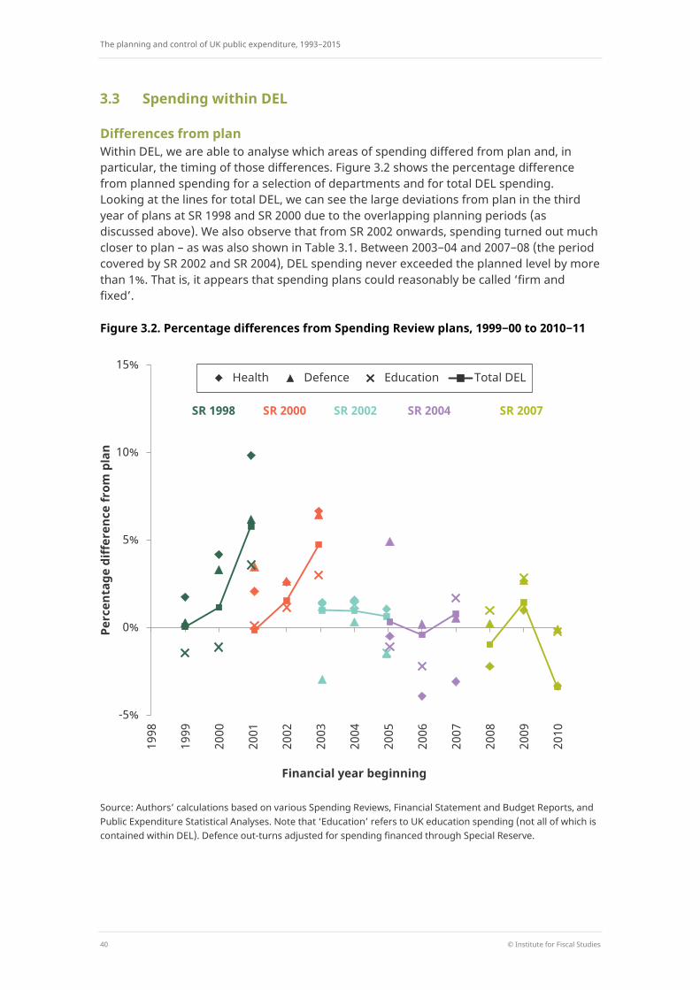
The planning and control of UK public expenditure, 1993−2015
40 © Institute for Fiscal Studies
3.3 Spending within DEL
Differences from plan Within DEL, we are able to analyse which areas of spending differed from plan and, in particular, the timing of those differences. Figure 3.2 shows the percentage difference from planned spending for a selection of departments and for total DEL spending. Looking at the lines for total DEL, we can see the large deviations from plan in the third year of plans at SR 1998 and SR 2000 due to the overlapping planning periods (as discussed above). We also observe that from SR 2002 onwards, spending turned out much closer to plan – as was also shown in Table 3.1. Between 2003−04 and 2007−08 (the period covered by SR 2002 and SR 2004), DEL spending never exceeded the planned level by more than 1%. That is, it appears that spending plans could reasonably be called ‘firm and fixed’.
Figure 3.2. Percentage differences from Spending Review plans, 1999−00 to 2010−11
Source: Authors’ calculations based on various Spending Reviews, Financial Statement and Budget Reports, and Public Expenditure Statistical Analyses. Note that ‘Education’ refers to UK education spending (not all of which is contained within DEL). Defence out-turns adjusted for spending financed through Special Reserve.
-5%
0%
5%
10%
15%
1998
1999
2000
2001
2002
2003
2004
2005
2006
2007
2008
2009
2010
Perc
enta
ge d
iffer
ence
from
pla
n
Financial year beginning
Health Defence Education Total DEL
SR 1998 SR 2000 SR 2002 SR 2004 SR 2007
The DEL/AME regime under Labour: 1999−00 to 2009−10
© Institute for Fiscal Studies 41
Box 3.1. Health spending
At its first Spending Review, of July 1998, the Labour government declared health to be a priority area of spending and announced a ‘massive investment’ into the NHS of more than £20 billion over three years, increasing funding at an average real rate of 4.7% per year up to 2001−02.
In January 2000, the Prime Minister expressed his aspiration to increase UK health spending to the EU average.a In March 2000, the Chancellor announced that he would be providing an additional £2 billion for 2000−01 (the second year of SR 1998 plans) and an extra £3.1 billion for 2001−02.b The 2001−02 allocation was then increased by a further £3.0 billion just a few months later in the July 2000 SR, forming the first year of the new plans. As a result, health spending in 2001−02 turned out nearly 10% higher than initially planned in SR 1998.
At the April 2002 Budget, in response to the recommendations of the Wanless Review of long-term health trends,c the government announced that UK NHS spending would grow by 7.4% per year over the five years to 2007−08. This longer planning period reflected the government’s acknowledgement of ‘the need to plan beyond the three-year horizons of firm DEL plans in specific areas’.d By 2007−08, UK health spending was projected to reach 9.4% of GDP, compared with the (2002) unweighted EU average of around 8%.e Expenditure increased slightly faster than planned, and SR 2004 rolled forward the plans with an additional £1.2 billion for 2005−06. However, from 2006−07 onwards, health spending failed to keep pace with plans – in stark contrast to previous years.
Splitting resource spending within health DEL (RDEL) from capital spending (CDEL) provides a more complete picture of the overspending (or top-ups) in the earlier part of the period and the undershooting of plans from 2006−07 onwards. The vast majority of health spending came under RDEL, out-turns and plans for which are shown in Figure 3.3a. It can be seen that health RDEL rose by more than planned between 1998−99 and 2005−06. Spending then rose broadly in line with plans, but tended to turn out slightly lower than planned, and markedly below plans in 2010−11. In contrast, Figure 3.3b shows that CDEL – which was a fraction of the size of RDEL – rose by more than originally planned at SR 1998, but then persistently came in lower than planned. In 2006−07, for instance, health capital spending turned out more than £2 billion below the level set out in plans published at SR 2004.
a Tony Blair’s comments on this were made on BBC Breakfast with Frost, 16 January 2000, and were repeated in parliament several days later (Hansard, 19 January 2000, column 837). b Financial Statement and Budget Report March 2000. These additional spending allocations referred to UK-wide NHS spending, as distinct from Department of Health allocations within DEL. c D, Wanless, Securing our Future Health: Taking a Long-Term View, Final Report, 2002 (https://www.yearofcare.co.uk/sites/default/files/images/Wanless.pdf). d Paragraph 6.13 of Financial Statement and Budget Report April 2002. e Paragraph 7.4 of 2002 Spending Review. Note that subsequent methodological changes to the calculation of GDP mean that spending as a percentage of GDP is lower when calculated today.

The planning and control of UK public expenditure, 1993−2015
42 © Institute for Fiscal Studies
Figure 3.3a. Health RDEL, 1998−99 to 2010−11
Source: Various Financial Statement and Budget Reports, Pre-Budget Reports, Spending Reviews and Public Expenditure Statistical Analyses. Series break in 2002 is due to the introduction of RAB. Out-turns for 2008−09 and 2009−10 are adjusted for classification changes resulting from the Clear Line of Sight Project.
Figure 3.3b. Health CDEL, 1998−99 to 2010−11
Source: Various Financial Statement and Budget Reports, Pre-Budget Reports, Spending Reviews and Public Expenditure Statistical Analyses.
30 40 50 60 70 80 90
100 110 120
1998
–99
1999
–00
2000
–01
2001
–02
2002
–03
2003
–04
2004
–05
2005
–06
2006
–07
2007
–08
2008
–09
2009
–10
2010
–11
£ bi
llion
Successive plans Concurrent out-turn (pre 2002) Concurrent out-turn (post 2002)
-1
0
1
2
3
4
5
6
7
1998
–99
1999
–00
2000
–01
2001
–02
2002
–03
2003
–04
2004
–05
2005
–06
2006
–07
2007
–08
2008
–09
2009
–10
2010
–11
£ bi
llion
Successive plans
Concurrent out-turn

The DEL/AME regime under Labour: 1999−00 to 2009−10
© Institute for Fiscal Studies 43
As well as deviations from overall DEL spending plans, Figure 3.2 plots differences from a small number of departmental spending plans. There was a clear tendency for health spending to turn out higher than originally planned, particularly at the start of the period. Health spending is explored in more detail in Box 3.1. Education spending turned out relatively close to plan over the period, showing neither a tendency to persistently undershoot nor overshoot plans between 1999−00 and 2010−11.
Defence spending over this period was repeatedly topped up to cover the costs associated with military operations in Afghanistan and Iraq.50 This was done through the creation of a Special Reserve at the Pre-Budget Report in November 2002, which made provisions for covering the cost of these commitments and other international obligations. These top-ups represented spending above and beyond that planned at spending reviews, which did not include the cost of temporary military engagements. As a result, defence spending repeatedly turned out considerably higher than originally planned, particularly between 2008−09 and 2010−11, when allocations from the Special Reserve were in excess of £4 billion in each year.
After stripping out allocations from the Special Reserve,51 the differences from plan for defence are relatively modest over the period (these are the results shown in Figure 3.2). Spending in 2001−02 and 2003−04 was more than 5% higher than planned in SR 1998 and SR 2000, respectively. But plans for each of these years were topped up in the overlapping spending review, to the extent that spending in 2003−04 turned out lower than the new plan set in SR 2002.
End-year flexibility Recall that as part of the government’s new framework for planning public expenditure, departments were allowed to carry forward 100% of unspent resources into the following financial year under an end-year flexibility (EYF) system. This was intended to bring an end to the ‘use it or lose it’ mindset associated with wasteful surges in spending at year-end.
We are unable to quantitatively assess the impact of the EYF reforms on the proportion (or efficiency) of spending taking place in the final month(s) of the year, due to a lack of data at a suitably granular level. However, we are able to analyse how the new EYF arrangements were used and by which departments.
Figure 3.4 illustrates the scale of the accumulated resource and capital underspends carried forward under the new EYF arrangements from 2001−02 to 2009−10 (the only years for which data are available). Resource spending within DEL far exceeds capital DEL, so it is unsurprising that we observe a greater amount of accumulated resource underspends under EYF than capital underspends. However, capital underspending was far greater in relative terms: almost £4.9 billion was carried forward from 2006−07 to 2007−08 (almost
50 For instance, the cost of military operations in Afghanistan, Iraq and the Wider Gulf exceeded £3.5 billion in
nominal terms in 2008−09, 2009−10 and 2010−11. Source: Authors’ calculations using table 6b of Ministry of Defence, ‘Finance and economics annual statistical bulletin: departmental resources 2017’ (https://www.gov.uk/government/statistics/defence-departmental-resources-2017) and HM Treasury GDP deflators, September 2017 (https://www.gov.uk/government/statistics/gdp-deflators-at-market-prices-and-money-gdp-september-2017-quarterly-national-accounts-september-2017).
51 Estimated allocations to defence from the Special Reserve are taken from successive Public Expenditure Statistical Analyses, ‘Changes in departmental budgets’ chapter.
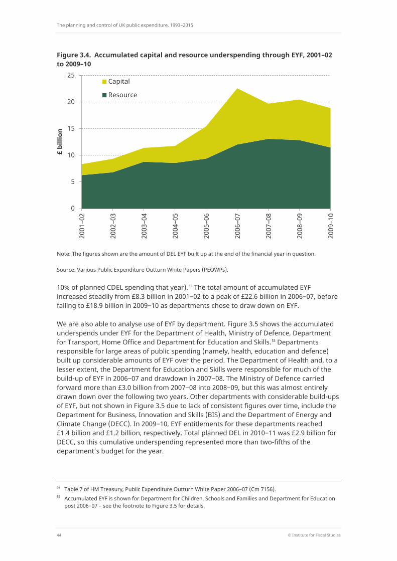
The planning and control of UK public expenditure, 1993−2015
44 © Institute for Fiscal Studies
Figure 3.4. Accumulated capital and resource underspending through EYF, 2001–02 to 2009–10
Note: The figures shown are the amount of DEL EYF built up at the end of the financial year in question.
Source: Various Public Expenditure Outturn White Papers (PEOWPs).
10% of planned CDEL spending that year).52 The total amount of accumulated EYF increased steadily from £8.3 billion in 2001−02 to a peak of £22.6 billion in 2006−07, before falling to £18.9 billion in 2009−10 as departments chose to draw down on EYF.
We are also able to analyse use of EYF by department. Figure 3.5 shows the accumulated underspends under EYF for the Department of Health, Ministry of Defence, Department for Transport, Home Office and Department for Education and Skills.53 Departments responsible for large areas of public spending (namely, health, education and defence) built up considerable amounts of EYF over the period. The Department of Health and, to a lesser extent, the Department for Education and Skills were responsible for much of the build-up of EYF in 2006−07 and drawdown in 2007−08. The Ministry of Defence carried forward more than £3.0 billion from 2007−08 into 2008−09, but this was almost entirely drawn down over the following two years. Other departments with considerable build-ups of EYF, but not shown in Figure 3.5 due to lack of consistent figures over time, include the Department for Business, Innovation and Skills (BIS) and the Department of Energy and Climate Change (DECC). In 2009−10, EYF entitlements for these departments reached £1.4 billion and £1.2 billion, respectively. Total planned DEL in 2010−11 was £2.9 billion for DECC, so this cumulative underspending represented more than two-fifths of the department’s budget for the year.
52 Table 7 of HM Treasury, Public Expenditure Outturn White Paper 2006−07 (Cm 7156). 53 Accumulated EYF is shown for Department for Children, Schools and Families and Department for Education
post 2006−07 – see the footnote to Figure 3.5 for details.
0
5
10
15
20
25 20
01–0
2
2002
–03
2003
–04
2004
–05
2005
–06
2006
–07
2007
–08
2008
–09
2009
–10
£ bi
llion
Capital
Resource
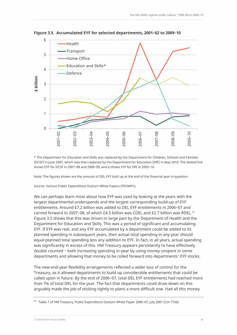
The DEL/AME regime under Labour: 1999−00 to 2009−10
© Institute for Fiscal Studies 45
Figure 3.5. Accumulated EYF for selected departments, 2001–02 to 2009–10
* The Department for Education and Skills was replaced by the Department for Children, Schools and Families (DCSF) in June 2007, which was then replaced by the Department for Education (DfE) in May 2010. The dotted line shows EYF for DCSF in 2007−08 and 2008−09, and it shows EYF for DfE in 2009−10.
Note: The figures shown are the amount of DEL EYF built up at the end of the financial year in question.
Source: Various Public Expenditure Outturn White Papers (PEOWPs).
We can perhaps learn most about how EYF was used by looking at the years with the largest departmental underspends and the largest corresponding build-up of EYF entitlements. Around £7.2 billion was added to DEL EYF entitlements in 2006−07 and carried forward to 2007−08, of which £4.5 billion was CDEL and £2.7 billion was RDEL.54 Figure 3.5 shows that this was driven in large part by the Department of Health and the Department for Education and Skills. This was a period of significant and accumulating EYF. If EYF was real, and any EYF accumulated by a department could be added to its planned spending in subsequent years, then actual total spending in any year should equal planned total spending less any addition to EYF. In fact, in all years, actual spending was significantly in excess of this. HM Treasury appears persistently to have effectively double counted – both increasing spending in-year by using money unspent in some departments and allowing that money to be rolled forward into departments’ EYF stocks.
The new end-year flexibility arrangements reflected a wider loss of control for the Treasury, as it allowed departments to build up considerable entitlements that could be called upon in future. By the end of 2006−07, total DEL EYF entitlements had reached more than 7% of total DEL for the year. The fact that departments could draw down on this arguably made the job of sticking tightly to plans a more difficult one. Had all this money
54 Table 7 of HM Treasury, Public Expenditure Outturn White Paper 2006−07, July 2007 (Cm 7156).
0
1
2
3
4
5
6
2001
–02
2002
–03
2003
–04
2004
–05
2005
–06
2006
–07
2007
–08
2008
–09
2009
–10
£ bi
llion
Health
Transport
Home Office
Education and Skills*
Defence
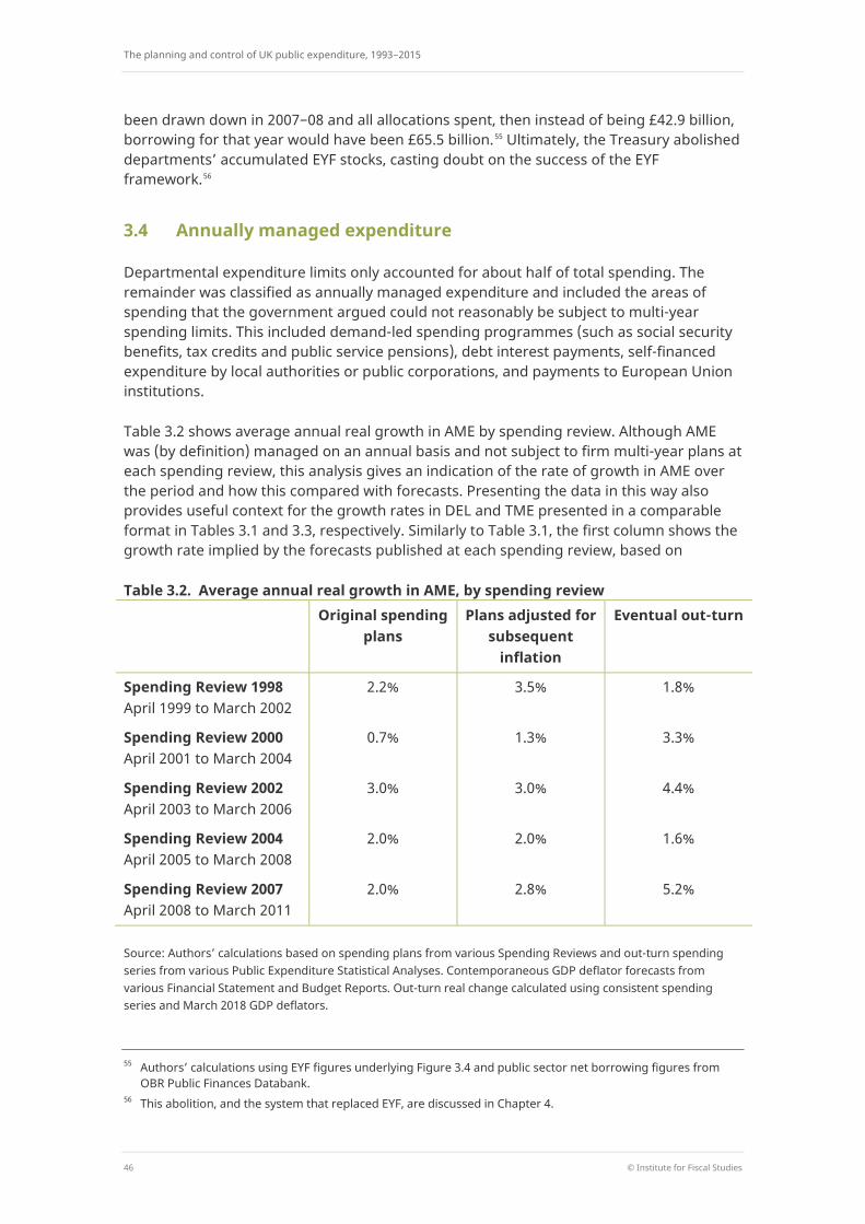
The planning and control of UK public expenditure, 1993−2015
46 © Institute for Fiscal Studies
been drawn down in 2007−08 and all allocations spent, then instead of being £42.9 billion, borrowing for that year would have been £65.5 billion.55 Ultimately, the Treasury abolished departments’ accumulated EYF stocks, casting doubt on the success of the EYF framework.56
3.4 Annually managed expenditure
Departmental expenditure limits only accounted for about half of total spending. The remainder was classified as annually managed expenditure and included the areas of spending that the government argued could not reasonably be subject to multi-year spending limits. This included demand-led spending programmes (such as social security benefits, tax credits and public service pensions), debt interest payments, self-financed expenditure by local authorities or public corporations, and payments to European Union institutions.
Table 3.2 shows average annual real growth in AME by spending review. Although AME was (by definition) managed on an annual basis and not subject to firm multi-year plans at each spending review, this analysis gives an indication of the rate of growth in AME over the period and how this compared with forecasts. Presenting the data in this way also provides useful context for the growth rates in DEL and TME presented in a comparable format in Tables 3.1 and 3.3, respectively. Similarly to Table 3.1, the first column shows the growth rate implied by the forecasts published at each spending review, based on
Table 3.2. Average annual real growth in AME, by spending review Original spending
plans Plans adjusted for
subsequent inflation
Eventual out-turn
Spending Review 1998 April 1999 to March 2002
2.2% 3.5% 1.8%
Spending Review 2000 April 2001 to March 2004
0.7% 1.3% 3.3%
Spending Review 2002 April 2003 to March 2006
3.0% 3.0% 4.4%
Spending Review 2004 April 2005 to March 2008
2.0% 2.0% 1.6%
Spending Review 2007 April 2008 to March 2011
2.0% 2.8% 5.2%
Source: Authors’ calculations based on spending plans from various Spending Reviews and out-turn spending series from various Public Expenditure Statistical Analyses. Contemporaneous GDP deflator forecasts from various Financial Statement and Budget Reports. Out-turn real change calculated using consistent spending series and March 2018 GDP deflators.
55 Authors’ calculations using EYF figures underlying Figure 3.4 and public sector net borrowing figures from
OBR Public Finances Databank. 56 This abolition, and the system that replaced EYF, are discussed in Chapter 4.
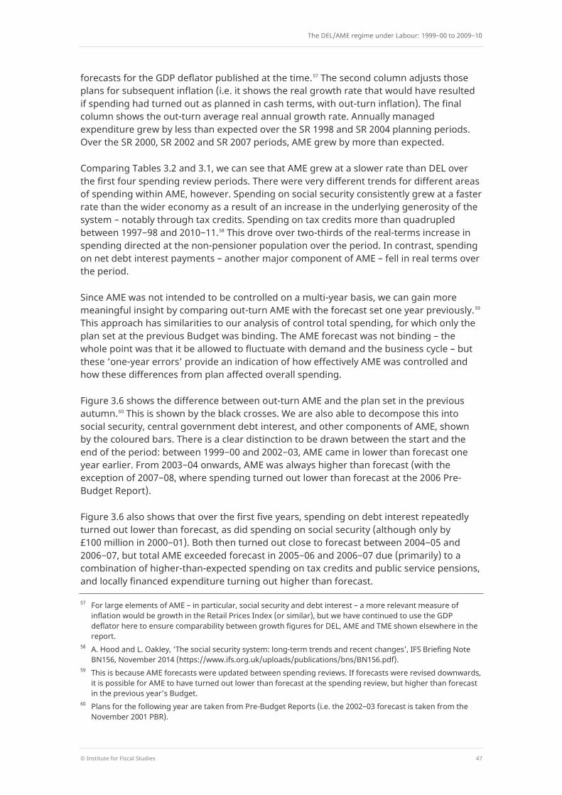
The DEL/AME regime under Labour: 1999−00 to 2009−10
© Institute for Fiscal Studies 47
forecasts for the GDP deflator published at the time.57 The second column adjusts those plans for subsequent inflation (i.e. it shows the real growth rate that would have resulted if spending had turned out as planned in cash terms, with out-turn inflation). The final column shows the out-turn average real annual growth rate. Annually managed expenditure grew by less than expected over the SR 1998 and SR 2004 planning periods. Over the SR 2000, SR 2002 and SR 2007 periods, AME grew by more than expected.
Comparing Tables 3.2 and 3.1, we can see that AME grew at a slower rate than DEL over the first four spending review periods. There were very different trends for different areas of spending within AME, however. Spending on social security consistently grew at a faster rate than the wider economy as a result of an increase in the underlying generosity of the system – notably through tax credits. Spending on tax credits more than quadrupled between 1997−98 and 2010−11.58 This drove over two-thirds of the real-terms increase in spending directed at the non-pensioner population over the period. In contrast, spending on net debt interest payments – another major component of AME – fell in real terms over the period.
Since AME was not intended to be controlled on a multi-year basis, we can gain more meaningful insight by comparing out-turn AME with the forecast set one year previously.59 This approach has similarities to our analysis of control total spending, for which only the plan set at the previous Budget was binding. The AME forecast was not binding – the whole point was that it be allowed to fluctuate with demand and the business cycle – but these ‘one-year errors’ provide an indication of how effectively AME was controlled and how these differences from plan affected overall spending.
Figure 3.6 shows the difference between out-turn AME and the plan set in the previous autumn.60 This is shown by the black crosses. We are also able to decompose this into social security, central government debt interest, and other components of AME, shown by the coloured bars. There is a clear distinction to be drawn between the start and the end of the period: between 1999−00 and 2002−03, AME came in lower than forecast one year earlier. From 2003−04 onwards, AME was always higher than forecast (with the exception of 2007−08, where spending turned out lower than forecast at the 2006 Pre-Budget Report).
Figure 3.6 also shows that over the first five years, spending on debt interest repeatedly turned out lower than forecast, as did spending on social security (although only by £100 million in 2000−01). Both then turned out close to forecast between 2004−05 and 2006−07, but total AME exceeded forecast in 2005−06 and 2006−07 due (primarily) to a combination of higher-than-expected spending on tax credits and public service pensions, and locally financed expenditure turning out higher than forecast.
57 For large elements of AME – in particular, social security and debt interest – a more relevant measure of
inflation would be growth in the Retail Prices Index (or similar), but we have continued to use the GDP deflator here to ensure comparability between growth figures for DEL, AME and TME shown elsewhere in the report.
58 A. Hood and L. Oakley, ‘The social security system: long-term trends and recent changes’, IFS Briefing Note BN156, November 2014 (https://www.ifs.org.uk/uploads/publications/bns/BN156.pdf).
59 This is because AME forecasts were updated between spending reviews. If forecasts were revised downwards, it is possible for AME to have turned out lower than forecast at the spending review, but higher than forecast in the previous year’s Budget.
60 Plans for the following year are taken from Pre-Budget Reports (i.e. the 2002−03 forecast is taken from the November 2001 PBR).
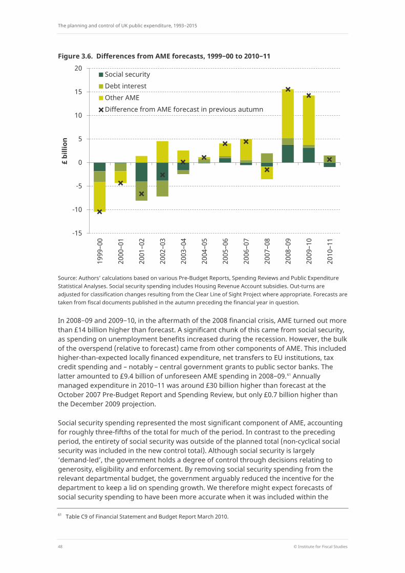
The planning and control of UK public expenditure, 1993−2015
48 © Institute for Fiscal Studies
Figure 3.6. Differences from AME forecasts, 1999−00 to 2010−11
Source: Authors’ calculations based on various Pre-Budget Reports, Spending Reviews and Public Expenditure Statistical Analyses. Social security spending includes Housing Revenue Account subsidies. Out-turns are adjusted for classification changes resulting from the Clear Line of Sight Project where appropriate. Forecasts are taken from fiscal documents published in the autumn preceding the financial year in question.
In 2008−09 and 2009−10, in the aftermath of the 2008 financial crisis, AME turned out more than £14 billion higher than forecast. A significant chunk of this came from social security, as spending on unemployment benefits increased during the recession. However, the bulk of the overspend (relative to forecast) came from other components of AME. This included higher-than-expected locally financed expenditure, net transfers to EU institutions, tax credit spending and – notably – central government grants to public sector banks. The latter amounted to £9.4 billion of unforeseen AME spending in 2008−09.61 Annually managed expenditure in 2010−11 was around £30 billion higher than forecast at the October 2007 Pre-Budget Report and Spending Review, but only £0.7 billion higher than the December 2009 projection.
Social security spending represented the most significant component of AME, accounting for roughly three-fifths of the total for much of the period. In contrast to the preceding period, the entirety of social security was outside of the planned total (non-cyclical social security was included in the new control total). Although social security is largely ‘demand-led’, the government holds a degree of control through decisions relating to generosity, eligibility and enforcement. By removing social security spending from the relevant departmental budget, the government arguably reduced the incentive for the department to keep a lid on spending growth. We therefore might expect forecasts of social security spending to have been more accurate when it was included within the
61 Table C9 of Financial Statement and Budget Report March 2010.
-15
-10
-5
0
5
10
15
20
1999
–00
2000
–01
2001
–02
2002
–03
2003
–04
2004
–05
2005
–06
2006
–07
2007
–08
2008
–09
2009
–10
2010
–11
£ bi
llion
Social security Debt interest Other AME Difference from AME forecast in previous autumn
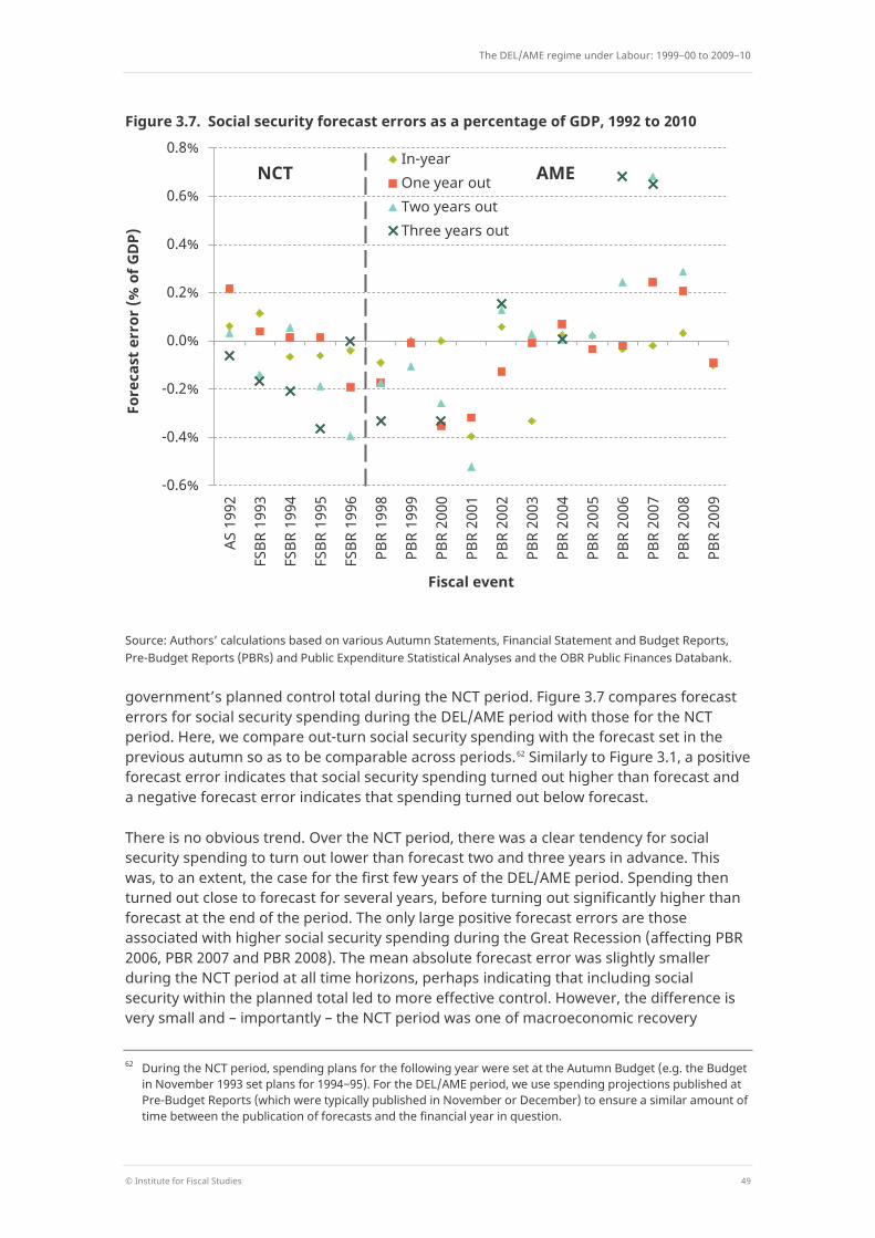
The DEL/AME regime under Labour: 1999−00 to 2009−10
© Institute for Fiscal Studies 49
Figure 3.7. Social security forecast errors as a percentage of GDP, 1992 to 2010
Source: Authors’ calculations based on various Autumn Statements, Financial Statement and Budget Reports, Pre-Budget Reports (PBRs) and Public Expenditure Statistical Analyses and the OBR Public Finances Databank.
government’s planned control total during the NCT period. Figure 3.7 compares forecast errors for social security spending during the DEL/AME period with those for the NCT period. Here, we compare out-turn social security spending with the forecast set in the previous autumn so as to be comparable across periods.62 Similarly to Figure 3.1, a positive forecast error indicates that social security spending turned out higher than forecast and a negative forecast error indicates that spending turned out below forecast.
There is no obvious trend. Over the NCT period, there was a clear tendency for social security spending to turn out lower than forecast two and three years in advance. This was, to an extent, the case for the first few years of the DEL/AME period. Spending then turned out close to forecast for several years, before turning out significantly higher than forecast at the end of the period. The only large positive forecast errors are those associated with higher social security spending during the Great Recession (affecting PBR 2006, PBR 2007 and PBR 2008). The mean absolute forecast error was slightly smaller during the NCT period at all time horizons, perhaps indicating that including social security within the planned total led to more effective control. However, the difference is very small and – importantly – the NCT period was one of macroeconomic recovery
62 During the NCT period, spending plans for the following year were set at the Autumn Budget (e.g. the Budget
in November 1993 set plans for 1994−95). For the DEL/AME period, we use spending projections published at Pre-Budget Reports (which were typically published in November or December) to ensure a similar amount of time between the publication of forecasts and the financial year in question.
-0.6%
-0.4%
-0.2%
0.0%
0.2%
0.4%
0.6%
0.8%
AS 1
992
FSBR
199
3
FSBR
199
4
FSBR
199
5
FSBR
199
6
PBR
1998
PBR
1999
PBR
2000
PBR
2001
PBR
2002
PBR
2003
PBR
2004
PBR
2005
PBR
2006
PBR
2007
PBR
2008
PBR
2009
Fore
cast
err
or (%
of G
DP)
Fiscal event
In-year One year out Two years out Three years out
NCT AME

The planning and control of UK public expenditure, 1993−2015
50 © Institute for Fiscal Studies
growth, without a major economic downturn and the associated surge in cyclical social security spending. We are therefore unable to draw any firm conclusions.
3.5 Total managed expenditure
Departmental expenditure limits and annually managed expenditure sum to give total managed expenditure, the government’s preferred measure of total public spending during this period. Table 3.3 summarises average annual real growth in TME by spending review.
Table 3.3. Average annual real growth in TME, by spending review Original spending
plans Plans adjusted for
subsequent inflation
Eventual out-turn
Spending Review 1998 April 1999 to March 2002
2.7% 4.0% 4.0%
Spending Review 2000 April 2001 to March 2004
3.2% 3.8% 5.7%
Spending Review 2002 April 2003 to March 2006
4.3% 4.3% 4.9%
Spending Review 2004 April 2005 to March 2008
3.2% 3.1% 2.9%
Spending Review 2007 April 2008 to March 2011
2.0% 2.8% 3.7%
Source: Authors’ calculations based on spending plans from various Spending Reviews and out-turn spending series from various Public Expenditure Statistical Analyses. Contemporaneous GDP deflator forecasts from various Financial Statement and Budget Reports. Out-turn real change calculated using consistent spending series and March 2018 GDP deflators.
After adjusting for subsequent inflation, TME grew in line with the plans set out at the 1998 Spending Review. Within the total, however, DEL grew by more than planned and AME by less (as shown in Tables 3.1 and 3.2). At the following two spending reviews, TME grew by more than planned, before growing in line with the plans set at the 2004 Spending Review. Between 2008−09 and 2010−11, public spending increased at almost twice the real rate originally planned at the 2007 Spending Review, driven in part by lower-than-expected inflation and in part by higher-than-forecast AME spending following the financial crisis and associated economic downturn.
3.6 Capital spending
Public sector net investment One of the key changes brought about by the introduction of the DEL/AME regime was the separation of the current (resource) components of departmental budgets from the capital budget for control purposes. This change was made to address the government’s concern that the lack of distinction between current and capital spending under the
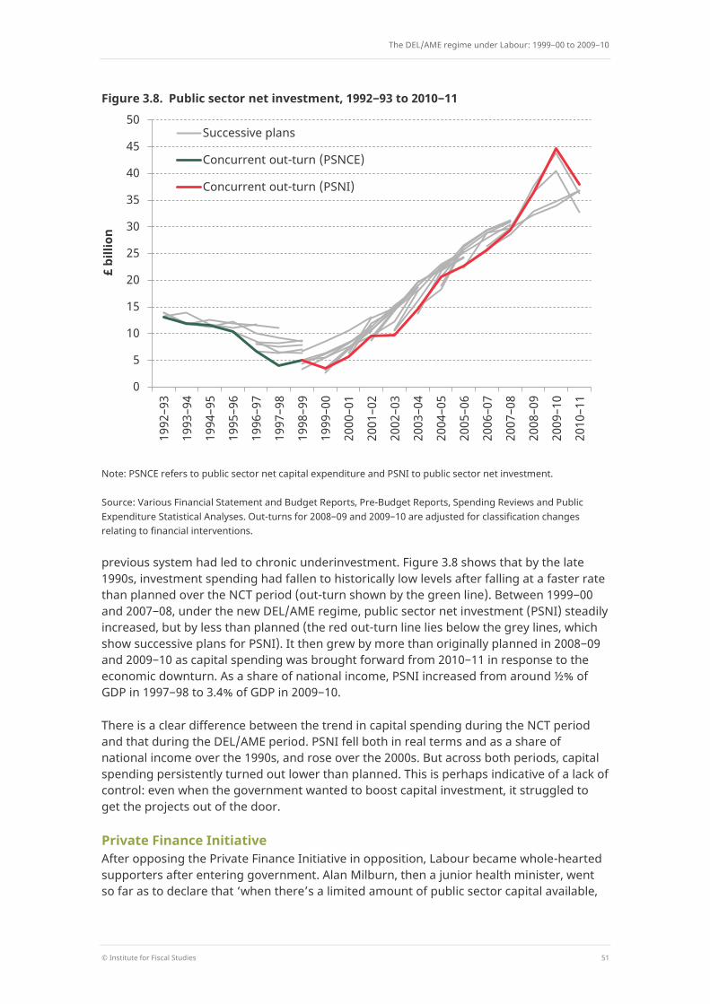
The DEL/AME regime under Labour: 1999−00 to 2009−10
© Institute for Fiscal Studies 51
Figure 3.8. Public sector net investment, 1992−93 to 2010−11
Note: PSNCE refers to public sector net capital expenditure and PSNI to public sector net investment.
Source: Various Financial Statement and Budget Reports, Pre-Budget Reports, Spending Reviews and Public Expenditure Statistical Analyses. Out-turns for 2008−09 and 2009−10 are adjusted for classification changes relating to financial interventions.
previous system had led to chronic underinvestment. Figure 3.8 shows that by the late 1990s, investment spending had fallen to historically low levels after falling at a faster rate than planned over the NCT period (out-turn shown by the green line). Between 1999−00 and 2007−08, under the new DEL/AME regime, public sector net investment (PSNI) steadily increased, but by less than planned (the red out-turn line lies below the grey lines, which show successive plans for PSNI). It then grew by more than originally planned in 2008−09 and 2009−10 as capital spending was brought forward from 2010−11 in response to the economic downturn. As a share of national income, PSNI increased from around ½% of GDP in 1997−98 to 3.4% of GDP in 2009−10.
There is a clear difference between the trend in capital spending during the NCT period and that during the DEL/AME period. PSNI fell both in real terms and as a share of national income over the 1990s, and rose over the 2000s. But across both periods, capital spending persistently turned out lower than planned. This is perhaps indicative of a lack of control: even when the government wanted to boost capital investment, it struggled to get the projects out of the door.
Private Finance Initiative After opposing the Private Finance Initiative in opposition, Labour became whole-hearted supporters after entering government. Alan Milburn, then a junior health minister, went so far as to declare that ‘when there’s a limited amount of public sector capital available,
0
5
10
15
20
25
30
35
40
45
50
1992
–93
1993
–94
1994
–95
1995
–96
1996
–97
1997
–98
1998
–99
1999
–00
2000
–01
2001
–02
2002
–03
2003
–04
2004
–05
2005
–06
2006
–07
2007
–08
2008
–09
2009
–10
2010
–11
£ bi
llion
Successive plans
Concurrent out-turn (PSNCE)
Concurrent out-turn (PSNI)
The planning and control of UK public expenditure, 1993−2015
52 © Institute for Fiscal Studies
it’s PFI or bust’.63 This commitment was reaffirmed in a July 2003 report, as ‘the PFI programme’s small but important role in the delivery of the Government’s investment plans’ was confirmed.64 The same report noted that both the number and capital value of PFI projects had increased, from nine projects with a total value of £667 million in 1995 to 65 projects with a total value of £7.6 billion in 2002.
We are unable to undertake comprehensive quantitative analysis of how capital spending under PFI compared with plans, or to assess the value for money of PFI. But PFI clearly played an important role in the government’s plans for investment in public services. PFI made up between 10% and 15% of total investment in public services between 1997−98 and 2003−04.65
One particular feature of the Private Finance Initiative is worthy of note. Under PFI, so long as certain risks are deemed to be passed to the private sector on a project, it is recorded off balance sheet for National Accounts and statistical purposes.66 This means that the bulk of PFI debt did not count towards public sector net debt (PSND). Recall that the government’s sustainable investment rule required the ratio of PSND to be kept below a ‘stable and prudent’ level (interpreted as 40% of GDP). By definition, anything that reduced the size of PSND would make this target easier to achieve. In 2005, IFS researchers estimated that in April 2004, public sector net debt would have been 1.2% of national income higher as a result of including on the public sector’s balance sheet the PFI investment that was on the private sector’s balance sheet at the time.67
The government insisted that the decision to undertake PFI investment (rather than ‘traditional’ public investment) was always taken on value-for-money grounds alone, and that whether it was on or off balance sheet was irrelevant to the choice of procurement route. Nonetheless, there was suspicion that deals were being structured in order to achieve a particular accounting treatment and flatter the public sector debt numbers in order to ‘game’ the fiscal rules.68
Private Finance Initiative payments were not the only liability held off-balance-sheet as a result of accounting classifications. Particularly notable was borrowing carried out by Network Rail, which was defined as a private sector company. This despite the fact the government guaranteed to repay Network Rail debt in the case of collapse, and held a great degree of control over its income through decisions over the prices paid by train operators to use its infrastructure. If Network Rail had been structured in part to game the government’s own fiscal rules, and there is good reason to believe this was at least part of what was going on, the behaviour ultimately turned out to be ineffective. In light of the switch to a new accounting standard (European System of Accounts 2010), the Office for National Statistics reclassified Network Rail as part of the public sector, and its debts
63 BBC News, 17 May 2001,
http://news.bbc.co.uk/news/vote2001/hi/english/main_issues/sections/facts/newsid_1182000/1182645.stm. 64 HM Treasury, PFI: Meeting the Investment Challenge, July 2003
(http://webarchive.nationalarchives.gov.uk/+/http://www.hm-treasury.gov.uk/media/F/7/PFI_604a.pdf). 65 Ibid. 66 Treasury Select Committee, Private Finance Initiative, Seventeenth Report, 2011
(https://publications.parliament.uk/pa/cm201012/cmselect/cmtreasy/1146/114602.htm). 67 R. Chote and C. Emmerson, ‘Fiscal policy framework’, in R. Chote, C. Emmerson, D. Miles and Z. Oldfield (eds),
The IFS Green Budget 2005, January 2005 (https://www.ifs.org.uk/publications/3250). 68 Ibid.
The DEL/AME regime under Labour: 1999−00 to 2009−10
© Institute for Fiscal Studies 53
(amounting to £30 billion in 2012–13) were brought back on to the public sector balance sheet in 2014. The need to focus on the underlying economic nature of spending of different kinds in controlling spending levels, deficit and debt is clear. The potential costs of structuring contracts simply to avoid artificial fiscal constraints are potentially large.
This is related to a wider concern over the government ‘fiddling’ its fiscal rules. For example, the so-called golden rule required an assessment of when the current economic cycle began. In June 2005, whether or not the golden rule was on course to be met over the economic cycle (which was thought to end in that financial year, 2005−06) depended on when the cycle was judged to have begun. If it had started in 1999−00, the rule was on course to be missed; if it had begun in 1997−98, the rule was on course to be met. In July 2005, Gordon Brown revised his previous judgement of when the cycle began from 1999−00 to 1997−98, despite the fact that the evidence for such a change seemed no stronger than before. This is perhaps a case of the government ‘moving the goalposts’ to stay within the letter, if not the spirit, of its fiscal rules, so that the government did not need to take decisions to rein in spending.
3.7 Conclusion
In the first few years of Gordon Brown’s chancellorship, spending plans were tight. In his first two years, Mr Brown successfully stayed within the spending limits set out by his predecessor, and general government expenditure fell from 40.3% of GDP in 1996−97 to 38.3% in 1998−99.69 In the year following the introduction of the DEL/AME spending framework, public expenditure continued to fall as a share of national income, with the Chancellor declaring his determination to be ‘prudent for a purpose’.70 Overall spending then increased steadily as a share of national income over the course of the 2000s, before increasing sharply following the financial crisis of 2008 and the associated recession.
There was a tendency for total managed expenditure (the government’s measure of overall public expenditure during the period) to increase at a faster rate than planned.71 Spending plans were set in cash terms, so lower-than-expected inflation meant that real spending was higher than originally envisaged. But total spending also turned out higher than planned in nominal terms over the 2000, 2002 and 2007 spending review periods.
The switch to the DEL/AME regime and the introduction of multi-year spending plans was intended to afford departments more certainty. The plans set for DEL at each spending review were intended to be ‘firm and fixed’ and not subject to biannual tinkering at each fiscal event. To an extent, this was achieved. Forecast errors for DEL were smaller than those for the control total at all time horizons. Even for plans set for the following year,
69 Public Expenditure Statistical Analyses 2000−01, April 2000. 70 Gordon Brown, Budget Speech, March 1998: ‘I said that this would be a Budget based on prudence for a
purpose and that guides us also in our approach to public spending’ (Hansard, 17 March 1998, vol. 308, cc1111–12).
71 The exception is Spending Review 2004, when real growth in TME was slightly lower than planned – see Table 3.3.
The planning and control of UK public expenditure, 1993−2015
54 © Institute for Fiscal Studies
when both NCT and DEL plans were ‘binding’, the mean absolute forecast error was more than three times as large during the NCT period.72
However, plans were not fully ‘firm and fixed’. The government was not able to resist making some incremental changes to its spending plans. This mainly happened at overlapping spending reviews, where plans for the third and final year of the previous SR would be reset and rolled forward. But spending was also ‘topped up’ between spending reviews, notably so at the Budgets of 2000, 2002 and 2009. Health spending in particular showed a tendency to be ‘topped up’ in the early part of the period.
Another feature of the new planning framework was the expansion of end-year flexibility arrangements, which saw departments build up considerable entitlements that would otherwise have been surrendered to the Treasury. The build-up of these entitlements implies that there were persistent underspends. Yet these underspends were effectively spent by Treasury, as indicated by the fact that there was continual topping-up of DELs and there were not undershoots against plans of the scale of the growing EYF entitlements.
The introduction of a Special Reserve in November 2002 was an important development which allowed the Treasury to fund the costs of military operations overseas without that temporary spending becoming ‘baked in’ to future Ministry of Defence budgets. Allocations from the Special Reserve represented the shifting of funds within DEL, so did not affect how total DEL fared relative to plan, but did lead to defence spending regularly turning out higher than originally planned.
One big difference between the DEL/AME and NCT regimes is in the proportion of spending that the government sought to ‘control’: whereas NCT spending represented around 85% of aggregate spending, DEL represented around half. A major component of the remainder, termed annually managed expenditure, was social security spending. Our analysis suggests that the mean absolute forecast error for social security spending was slightly lower during the NCT period, but this difference at two- and three-year horizons disappears if we exclude the period of the financial crisis (when spending on benefits increased as a result of the economic downturn).
One of the new Labour government’s priorities was to boost investment spending, which had fallen to historically low levels by 1997−98. However, over the government’s first term, public sector net investment remained broadly flat as a share of national income, and the four years from 1997−98 to 2000−01 were the lowest four-year period of investment spending since the Second World War. Investment spending did then begin to rise – albeit at a slower rate than planned – before sharply increasing in 2008−09 and 2009−10 as capital spending was brought forward from 2010−11 in response to the economic downturn. Overall, this indicates that the Treasury continued to struggle to effectively control capital spending and deliver the government’s investment plans.
Over this period, there was some concern that the government showed a tendency to ‘move the goalposts’ so as to meet its fiscal rules over this period – notably by re-dating the economic cycle to meet the golden rule – and to be influenced by the accounting
72 The mean one-year absolute forecast error for the adjusted NCT (i.e. with social security and local authority
self-financed expenditure) was 0.36% of GDP, as compared with 0.11% of GDP for DEL between 1999−00 and 2008–09.
The DEL/AME regime under Labour: 1999−00 to 2009−10
© Institute for Fiscal Studies 55
treatment of different types of spending when making decisions. One important conclusion to draw from this period is that meeting, or coming close to meeting, specified targets over a period of years is not necessarily the same as exercising effective spending control. The combination of failure to meet capital spending commitments, gaming fiscal rules and time-inconsistent use of end-year flexibility arguably meant that some of the apparent close control of spending was illusory. Of course, the real, if unanticipated, illusion was uncovered by the financial crisis. It turned out that spending levels were not sustainable because economic performance was not sustainable.

The planning and control of UK public expenditure, 1993−2015
56 © Institute for Fiscal Studies
4. The DEL/AME regime under austerity: 2010−11 to 2015−16
4.1 Introduction
The Conservative–Liberal-Democrat coalition government entered office in 2010 aiming to reduce public sector borrowing in the wake of the financial crisis, largely through cuts to public spending. In the June 2010 Budget forecast, TME was projected to fall from 47.5% of GDP in 2009−10 to 40.9% of GDP in 2014−15, a reduction of 6.6% of GDP over a five-year period.73 This was substantially larger than the fiscal consolidation planned by the Conservatives in the 1990s: at the November 1993 Budget (the first at which the Conservatives announced real spending cuts), general government expenditure was projected to fall by approximately 3.0% of GDP over the five years to 1997−98.74
The new fiscal rules The new era of fiscal contraction was accompanied by a new set of fiscal rules that set out the path by which the Treasury planned to return the public finances to a sustainable footing. The coalition government introduced two fiscal targets on coming to power in 2010:75
1. The fiscal mandate: the structural current budget (that is, borrowing for non-investment spending, after adjusting for the economic cycle) must be forecast to be in balance or in surplus by the end of the rolling, five-year forecast horizon.
2. The supplementary target: public sector net debt as a share of national income should be lower in 2015−16 than in 2014−15.
The fiscal mandate was similar in spirit to the golden rule of the previous Labour government. Both allowed the government to borrow to fund investment spending, and both allowed borrowing to take into account the ups and downs of the economic cycle. The main difference is one of timing – the golden rule judged borrowing over an economic cycle (with the difficulty that that required a cycle to be dated, and contemporaneously), while the fiscal mandate was forward looking.
While these rules constrained the government to have fiscal plans in place that would restore public borrowing to sustainable levels, the ‘rolling’ forward-looking nature of the fiscal mandate provided flexibility at the potential cost of credibility. Each Autumn
73 Table C6 of Office for Budget Responsibility, Budget forecast, June 2010
(http://obr.uk/docs/junebudget_annexc.pdf). 74 The November 1993 Budget published spending plans for the three years up to 1996−97, along with
projections for GGE as a share of GDP (table 5B.1). We extrapolate these projections using the plans announced at the November 1994 Budget to calculate the estimated reduction in GGE as a share of GDP between 1992−93 and 1997−98.
75 The golden rule and the sustainable investment rule of the 2000s had already been suspended by the previous Labour government in 2008, and replaced in 2010 by the Fiscal Responsibility Act. This is discussed in more detail in C. Emmerson, S. Keynes and G. Tetlow, ‘The fiscal targets’, in C. Emmerson, P. Johnson and H. Miller (eds), The IFS Green Budget: February 2013 (https://www.ifs.org.uk/budgets/gb2013/GB2013_Ch4.pdf).

The DEL/AME regime under austerity: 2010−11 to 2015−16
© Institute for Fiscal Studies 57
Statement, the end of the forecast horizon moved forwards one year, potentially giving the government the option to delay reaching structural current budget balance.
At the end of 2014, the government updated its fiscal rules: the fiscal mandate was changed to look forward three years rather than five, while the supplementary target was changed to focus on the path of debt between 2015−16 and 2016−17 rather than 2014−15 and 2015−16. (After the 2015 election, the Conservative government introduced a new mandate for fiscal policy, with a target of reaching a surplus on public sector net borrowing by the end of 2019−20, and a pledge to maintain a surplus each year thereafter so long as the economy was judged to be ‘in normal times’.)
It is worth noting that since 2010 the various fiscal mandates have continued to target fiscal aggregates that do not incorporate financial transactions and other ‘non-cash’ spending. This has led to some concern that the government is incentivised to meet the letter rather than the spirit of the fiscal rules, by focusing on policies that – because of their accounting treatment – affect measured borrowing in a way that is different from their true long-run cost. This is applicable to, for example, loans made to students and businesses, and government guarantees to the private sector, which are likely to ultimately involve a (sometimes substantial) public subsidy.
Other changes to the planning regime The system for the planning and control of public spending was broadly maintained by the new government. The distinction between DEL and AME was kept, as was the division of budgets into separate current (resource) and capital components, and the spending review process. The government did, however, make a few adjustments.
Lack of incentive to control AME and the welfare cap The government was concerned that because AME was not subject to firm limits,76 departments did not have the same incentives to manage it, which it argued weakened spending control. In oral evidence to the Treasury Select Committee in November 2010, George Osborne explained:
I think that’s one of the big challenges facing the Treasury, the annually managed expenditure bill, because there has been no incentive on Government Departments to control those budgets. We are looking at whether this whole framework of DEL-AME needs to be revisited, particularly the AME part of it, because this is a very large budget – I think virtually half of Government spending. Although it’s called ‘annually managed expenditure’, it’s not really managed. So we are looking at a new framework.77
The 2013 Spending Round announced that welfare, or social security, spending would be subject to a cap.78 The cap was designed so as to exclude spending on the state pension
76 By its initial definition, AME could not ‘reasonably be subject to firm multi-year limits’. 77 Treasury Select Committee, Examination of Witnesses, Spending Review 2010
(https://publications.parliament.uk/pa/cm201011/cmselect/cmtreasy/544/10110402.htm). 78 Social security was by far the largest element of AME. For example, in 2012−13, social security accounted for
53.8% of public sector current expenditure (PSCE) in AME, with tax credits accounting for a further 8.4%. Source: table 4.17 of Office for Budget Responsibility, Economic and Fiscal Outlook, March 2014 (Cm 8820).
The planning and control of UK public expenditure, 1993−2015
58 © Institute for Fiscal Studies
(which represented around 40% of total welfare spending in 2013−14) and some counter-cyclical elements of welfare, such as jobseeker’s allowance (JSA) and housing benefit paid to unemployed people.
In each Autumn Statement, the Office for Budget Responsibility was to assess whether the government was complying with the cap. If forecast spending on the covered areas exceeded the cap, the Chancellor would have to either cut spending or win a parliamentary vote to increase the level of the cap. The cap also included a ‘forecast margin’ of 2%, which allowed spending to be up to 2% higher than the cap due to forecasting changes. This allowed for small fluctuations in forecast without triggering a policy response, but if the forecast margin was breached, the same rules would apply.
The intention was to improve the degree of control over a major component of AME and ‘ensure that the welfare system remains affordable’.79 The rationale behind the cap was the perception that governments find it difficult to curb unexpected and unplanned increases in benefit spending since this requires unpopular decisions about how to make the benefit system less generous. By introducing a cap, governments would be forced to make active decisions about a desirable level of welfare spending, rather than allowing it passively to drift upwards. This, along with the inclusion of large elements of AME within the spending review envelope (discussed below), represented an attempt to exert greater control over spending outside departmental budgets.
Large build-up of EYF and the introduction of budget exchange Under the end-year flexibility (EYF) system, departments were able to carry forward unspent provision into future years, and these underspends accumulated over time. In 2009−10, these accumulated stocks amounted to almost £19 billion.80 If this stock was spent by departments, it would represent a considerable increase in expenditure and would mean additional borrowing.
The 2010 Spending Review announced that the EYF scheme would be abolished at the end of 2010−11, including all accumulated stocks, and replaced with a new system from the following year which would ‘retain an incentive for departments to avoid wasteful end-year spending and strengthen spending control’.81 The Budget of March 2011 announced that a new ‘budget exchange’ system would replace EYF. The new system allowed ‘departments to surrender an underspend in advance of the end of the financial year in return for a corresponding increase in their budget the following year, subject to a prudent limit’.82 The new system also included features intended to prevent the accumulation of spending power over time, by requiring any carry-forward from the previous year to be netted off the amount that could be carried forward into the next year. The new budget exchange system was intended to provide departments with flexibility to efficiently manage their budgets, while strengthening HM Treasury’s control of spending.
79 HM Treasury, Spending Round 2013, June 2013 (Cm 8639). 80 HM Treasury, Public Expenditure Provisional Outturn 2009−10, July 2010 (Cm 7911). 81 Paragraph 1.17 of HM Treasury, Spending Review 2010, October 2010 (Cm 7942). 82 Paragraph 2.9 of HM Treasury, Budget 2011, March 2011 (HC 836).

The DEL/AME regime under austerity: 2010−11 to 2015−16
© Institute for Fiscal Studies 59
Changes to spending reviews ‘The Spending Review framework’, published in June 2010, set out the new government’s approach to the forthcoming spending review, including its scope.83 As well as announcing its plans for a ‘step change in public sector productivity and value for money’, the document announced that for the first time, the spending review would look ‘comprehensively across the whole of Government expenditure’ and cover significant elements of AME, in addition to DELs. Within AME, social security, tax credits and public service pensions were to be included, while central government debt interest, BBC domestic services, National Lottery and net expenditure transfers to the EU were to be excluded. The intention was to bring elements of AME where the risk is taken by the exchequer as a whole within the scope of the spending review process so as to exert greater control. This meant that of the £701.8 billion of planned TME in 2011−12, £641.6 billion (91.4%) was within the spending envelope for Spending Review 2010.84
The new government also departed from the three-year planning periods of both the NCT regime and the DEL/AME regime under the Labour government. The 2010 Spending Review set out spending plans for the entire parliament, covering the four years from 2011−12 to 2014−15. A longer planning horizon gives more certainty to departments (in this case, more certainty over the scale of cuts the department would need to make) and enables multi-year pay deals. But it also reduces the ability of governments to alter public spending if the economic situation turns out different from prior forecasts – if the plans are indeed fixed. Conversely, the 2013 Spending Review set out spending plans for just one additional year, 2015–16, leaving the spending plans for the rest of the forecast horizon to be made after the next general election (which was to be held in May 2015).
Independence and the Office for Budget Responsibility Within days of coming to power in May 2010, the coalition government also established a new body, the Office for Budget Responsibility (OBR). The aim was to improve the credibility of government forecasts and wider fiscal policy.
Previously, the government’s forecasts for the economy and the public finances were produced in the Treasury. During the NCT period, the government convened a Panel of Independent Forecasters (the so-called ‘six wise men’) and would take into account the range of their estimates when deciding on an official forecast. Under Labour, the National Audit Office audited the economic assumptions underlying the Treasury forecast, assessing whether they were ‘reasonable’. In each case, the Chancellor retained a degree of influence over the precise forecast, which led to suspicion that forecasts may be persistently over-optimistic. Part of the rationale for the creation of the OBR was to address the perception that forecasts could be politically motivated by making the production process independent of government.
The OBR also comments on the government’s performance against its targets for the public finances, examines the long-term sustainability of the public finances, and analyses risks surrounding the public finances and trends in welfare spending.
83 HM Treasury, ‘The Spending Review framework’, 8 June 2010 (Cm 7872). 84 Table 1.1 of HM Treasury, Spending Review 2010, October 2010 (Cm 7942).
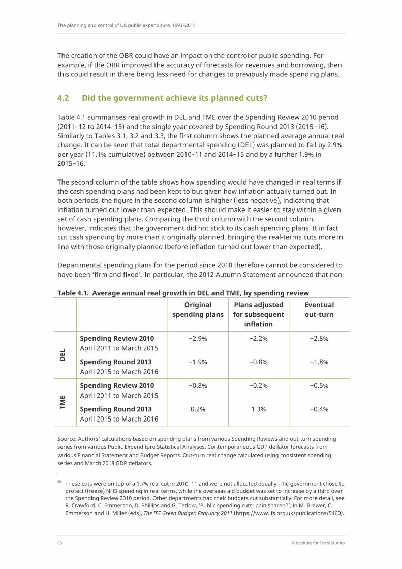
The planning and control of UK public expenditure, 1993−2015
60 © Institute for Fiscal Studies
The creation of the OBR could have an impact on the control of public spending. For example, if the OBR improved the accuracy of forecasts for revenues and borrowing, then this could result in there being less need for changes to previously made spending plans.
4.2 Did the government achieve its planned cuts?
Table 4.1 summarises real growth in DEL and TME over the Spending Review 2010 period (2011−12 to 2014−15) and the single year covered by Spending Round 2013 (2015−16). Similarly to Tables 3.1, 3.2 and 3.3, the first column shows the planned average annual real change. It can be seen that total departmental spending (DEL) was planned to fall by 2.9% per year (11.1% cumulative) between 2010–11 and 2014−15 and by a further 1.9% in 2015−16.85
The second column of the table shows how spending would have changed in real terms if the cash spending plans had been kept to but given how inflation actually turned out. In both periods, the figure in the second column is higher (less negative), indicating that inflation turned out lower than expected. This should make it easier to stay within a given set of cash spending plans. Comparing the third column with the second column, however, indicates that the government did not stick to its cash spending plans. It in fact cut cash spending by more than it originally planned, bringing the real-terms cuts more in line with those originally planned (before inflation turned out lower than expected).
Departmental spending plans for the period since 2010 therefore cannot be considered to have been ‘firm and fixed’. In particular, the 2012 Autumn Statement announced that non-
Table 4.1. Average annual real growth in DEL and TME, by spending review Original
spending plans Plans adjusted for subsequent
inflation
Eventual out-turn
DEL
Spending Review 2010 April 2011 to March 2015
−2.9% −2.2% −2.8%
Spending Round 2013 April 2015 to March 2016
−1.9% −0.8% −1.8%
TME
Spending Review 2010 April 2011 to March 2015
−0.8% −0.2% −0.5%
Spending Round 2013 April 2015 to March 2016
0.2% 1.3% −0.4%
Source: Authors’ calculations based on spending plans from various Spending Reviews and out-turn spending series from various Public Expenditure Statistical Analyses. Contemporaneous GDP deflator forecasts from various Financial Statement and Budget Reports. Out-turn real change calculated using consistent spending series and March 2018 GDP deflators.
85 These cuts were on top of a 1.7% real cut in 2010−11 and were not allocated equally. The government chose to
protect (freeze) NHS spending in real terms, while the overseas aid budget was set to increase by a third over the Spending Review 2010 period. Other departments had their budgets cut substantially. For more detail, see R. Crawford, C. Emmerson, D. Phillips and G. Tetlow, ‘Public spending cuts: pain shared?’, in M. Brewer, C. Emmerson and H. Miller (eds), The IFS Green Budget: February 2011 (https://www.ifs.org.uk/publications/5460).

The DEL/AME regime under austerity: 2010−11 to 2015−16
© Institute for Fiscal Studies 61
ring-fenced86 departmental resource budgets would be reduced by 1% in 2013−14 and by 2% in 2014−15 to achieve savings of £980 million and £2.4 billion respectively. At the March 2013 Budget, the government announced further cuts to DEL of £1.1 billion in 2013−14 and £1.2 billion in 2014−15, equivalent to a 1% reduction for most departments. Further cuts were then announced in December of that year at the Autumn Statement, with a 1.1% reduction in RDEL budgets in 2014−15 and 2015−16. In July 2015, the government announced an additional £2.6 billion of cuts within DEL for the 2015−16 financial year in progress. While the overall picture for the period was of repeated ‘top-slicing’ of departmental budgets, some departments did fare better than others. The health budget was protected and increased in real terms over the period87 and, unlike other departments, was increased between spending reviews rather than cut. For instance, the 2014 Autumn Statement announced an extra £2 billion for front-line NHS services in 2015−16.
Despite sizeable cuts to working-age welfare and other changes to spending areas outside of DEL, the government did not plan a real-terms reduction in AME between 2010 and 2015. Between 2010–11 and 2014−15, this meant that total spending (TME) was planned to fall by an average of 0.8% per year (compared with 2.9% per year for DEL). In 2015−16, TME was planned to increase by 0.2% in real terms.
Because inflation turned out lower than expected, had the government spent exactly as much as it planned to, TME would have in fact fallen by an average of 0.2% per year between 2010–11 and 2014−15 and increased by 1.3% in 2015−16 (the second column in Table 4.1). Out-turn data tell us that over both spending review periods, TME fell in real terms and that real growth was lower than if the government had stuck to its cash spending plans.
Underspends and budget exchange A key feature of the government’s spending control framework was its new system for inter-year spending flexibility, known as budget exchange, which operated from 2011−12 onwards. The new system meant that departments had to declare any underspends in advance of the end of the financial year and surrender them to the Treasury. Any underspends above and beyond those declared to the Treasury could not be carried forward to future years. So departments had a clear incentive to accurately assess their likely underspend for the year and to limit any underspending beyond that. Despite this, we observe considerable unanticipated departmental underspending over the period.
Table 4.2 uses OBR figures to show the estimated amount spent using money carried forward from earlier years under budget exchange for both departmental resource and capital spending (shown in the first two columns).88 For example, the figures 0.6 and 0.2 in
86 Health and schools spending continued to be protected. The government also chose to exempt local
government in 2013−14 and HMRC in both years. International development spending, whilst protected, fell as a result of a downgrade to forecasts for gross national income (as the government now needed to spend less in cash terms to hit its 0.7% target).
87 Out-turn data show that UK spending on health increased in real terms between 2010−11 and 2015−16, but fell in 2011−12. Source: table 4.3 of Public Expenditure Statistical Analyses 2017.
88 Note that rather than using Treasury definitions of RDEL and CDEL, the OBR instead uses ‘public sector current expenditure in RDEL’ and ‘public sector gross investment in CDEL’, which are broadly comparable but exclude a small number of items. A reconciliation table is published in the supplementary fiscal tables at each Economic and Fiscal Outlook.
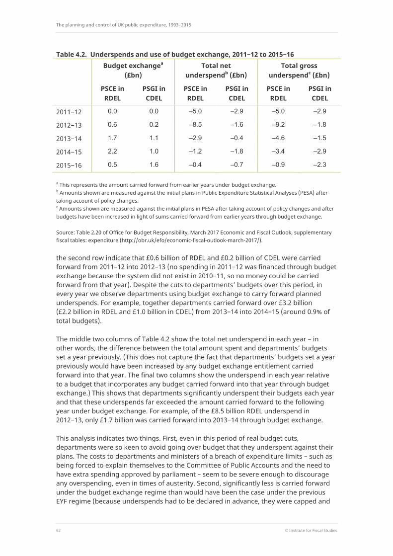
The planning and control of UK public expenditure, 1993−2015
62 © Institute for Fiscal Studies
Table 4.2. Underspends and use of budget exchange, 2011−12 to 2015−16 Budget exchangea
(£bn) Total net
underspendb (£bn) Total gross
underspendc (£bn)
PSCE in RDEL
PSGI in CDEL
PSCE in RDEL
PSGI in CDEL
PSCE in RDEL
PSGI in CDEL
2011−12 0.0 0.0 –5.0 –2.9 –5.0 –2.9
2012−13 0.6 0.2 –8.5 –1.6 –9.2 –1.8
2013−14 1.7 1.1 –2.9 –0.4 –4.6 –1.5
2014−15 2.2 1.0 –1.2 –1.8 –3.4 –2.9
2015−16 0.5 1.6 –0.4 –0.7 –0.9 –2.3
a This represents the amount carried forward from earlier years under budget exchange. b Amounts shown are measured against the initial plans in Public Expenditure Statistical Analyses (PESA) after taking account of policy changes. c Amounts shown are measured against the initial plans in PESA after taking account of policy changes and after budgets have been increased in light of sums carried forward from earlier years through budget exchange.
Source: Table 2.20 of Office for Budget Responsibility, March 2017 Economic and Fiscal Outlook, supplementary fiscal tables: expenditure (http://obr.uk/efo/economic-fiscal-outlook-march-2017/).
the second row indicate that £0.6 billion of RDEL and £0.2 billion of CDEL were carried forward from 2011–12 into 2012–13 (no spending in 2011−12 was financed through budget exchange because the system did not exist in 2010−11, so no money could be carried forward from that year). Despite the cuts to departments’ budgets over this period, in every year we observe departments using budget exchange to carry forward planned underspends. For example, together departments carried forward over £3.2 billion (£2.2 billion in RDEL and £1.0 billion in CDEL) from 2013−14 into 2014−15 (around 0.9% of total budgets).
The middle two columns of Table 4.2 show the total net underspend in each year – in other words, the difference between the total amount spent and departments’ budgets set a year previously. (This does not capture the fact that departments’ budgets set a year previously would have been increased by any budget exchange entitlement carried forward into that year. The final two columns show the underspend in each year relative to a budget that incorporates any budget carried forward into that year through budget exchange.) This shows that departments significantly underspent their budgets each year and that these underspends far exceeded the amount carried forward to the following year under budget exchange. For example, of the £8.5 billion RDEL underspend in 2012−13, only £1.7 billion was carried forward into 2013−14 through budget exchange.
This analysis indicates two things. First, even in this period of real budget cuts, departments were so keen to avoid going over budget that they underspent against their plans. The costs to departments and ministers of a breach of expenditure limits – such as being forced to explain themselves to the Committee of Public Accounts and the need to have extra spending approved by parliament – seem to be severe enough to discourage any overspending, even in times of austerity. Second, significantly less is carried forward under the budget exchange regime than would have been the case under the previous EYF regime (because underspends had to be declared in advance, they were capped and

The DEL/AME regime under austerity: 2010−11 to 2015−16
© Institute for Fiscal Studies 63
they could not be cumulated over time). This has strengthened the Treasury’s control over departments’ ability to shift spending across years, and removed the risk of departments driving total public spending higher than planned through their use of claims on accumulated EYF entitlements.
Social security and the welfare cap As previously described, another change the coalition government made to the DEL/AME regime was the introduction of a welfare spending cap. Since this was only in place towards the very end of our period, a meaningful quantitative analysis of its impact is not possible. However, the welfare cap has not been credible almost since its introduction. The level of the cap was first set in March 2014, and was then lowered in the July 2015 Budget after the new Conservative government introduced a number of policies intended to reduce benefit spending. However, in November 2015, the OBR forecast that the welfare cap would be breached in 2016−17 to 2018−19 (inclusive). In response, the Chancellor chose not to take action to reduce spending or ask permission to increase the cap – he simply explained to parliament why the breach was justified. This suggests that the change to the DEL/AME regime, in terms of the introduction of the welfare cap, has had little effect on the ability of the government to control social security spending.
Transfers between resource and capital budgets One of the features of the DEL/AME regime when it was introduced in 1998 was the separation of budgets into resource and current components. To address the perceived bias against capital spending, departments were unable to use the part of their budgets allocated to capital spending to fund day-to-day spending. However, since 2010, there have been several instances when the Treasury has allowed funding to be shifted from capital budgets in order to meet immediate spending pressures. For instance, in 2015−16, on top of the extra funding announced in the 2014 Autumn Statement, the Department of Health switched around £1.2 billion from CDEL to RDEL.89 This is not indicative of a lack of control per se – such transfers are sanctioned by the Treasury. However, it is indicative of the Treasury’s planned spending cuts being difficult to implement, and of unusual measures having to be taken in order for the planned resources budgets to be kept to. It is also perhaps indicative that the change in the government’s fiscal rules in 2015, from targeting a current budget balance (i.e. allowing borrowing to fund investment) to targeting an overall budget balance (i.e. allowing no borrowing), may have had real implications for the implementation of capital spending plans. One might suspect transfers from CDEL to RDEL would have been viewed less favourably by the Treasury if they made the government’s overall fiscal targets harder to meet.
Capital spending The planned cuts to departmental capital budgets over the period 2010–11 to 2015–16 were considerably deeper than those to resource budgets. Over the Spending Review 2010 period (the four years to 2014−15), CDEL was planned to fall by 29.1% in real terms, compared with 8.3% for RDEL. At the November 2010 Economic and Fiscal Outlook, the
89 Page 47 of Public Expenditure Statistical Analyses 2015 and page 46 of Public Expenditure Statistical Analyses
2016.
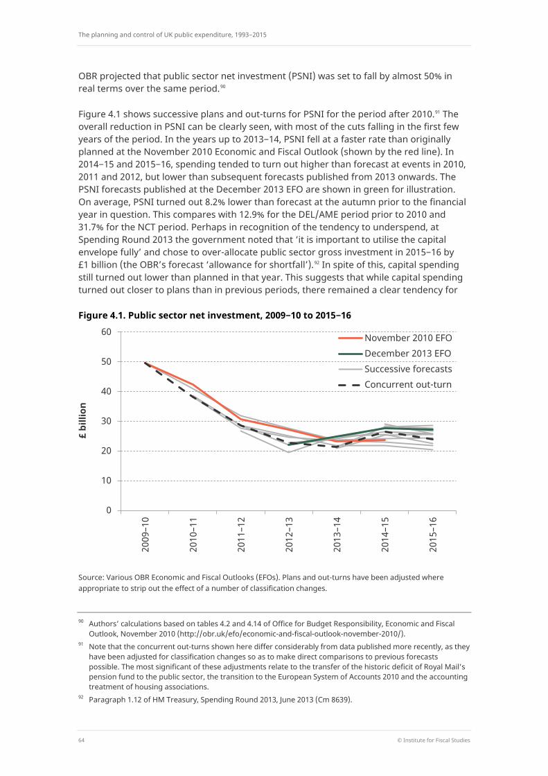
The planning and control of UK public expenditure, 1993−2015
64 © Institute for Fiscal Studies
OBR projected that public sector net investment (PSNI) was set to fall by almost 50% in real terms over the same period.90
Figure 4.1 shows successive plans and out-turns for PSNI for the period after 2010.91 The overall reduction in PSNI can be clearly seen, with most of the cuts falling in the first few years of the period. In the years up to 2013−14, PSNI fell at a faster rate than originally planned at the November 2010 Economic and Fiscal Outlook (shown by the red line). In 2014−15 and 2015−16, spending tended to turn out higher than forecast at events in 2010, 2011 and 2012, but lower than subsequent forecasts published from 2013 onwards. The PSNI forecasts published at the December 2013 EFO are shown in green for illustration. On average, PSNI turned out 8.2% lower than forecast at the autumn prior to the financial year in question. This compares with 12.9% for the DEL/AME period prior to 2010 and 31.7% for the NCT period. Perhaps in recognition of the tendency to underspend, at Spending Round 2013 the government noted that ‘it is important to utilise the capital envelope fully’ and chose to over-allocate public sector gross investment in 2015−16 by £1 billion (the OBR’s forecast ‘allowance for shortfall’).92 In spite of this, capital spending still turned out lower than planned in that year. This suggests that while capital spending turned out closer to plans than in previous periods, there remained a clear tendency for
Figure 4.1. Public sector net investment, 2009−10 to 2015−16
Source: Various OBR Economic and Fiscal Outlooks (EFOs). Plans and out-turns have been adjusted where appropriate to strip out the effect of a number of classification changes.
90 Authors’ calculations based on tables 4.2 and 4.14 of Office for Budget Responsibility, Economic and Fiscal
Outlook, November 2010 (http://obr.uk/efo/economic-and-fiscal-outlook-november-2010/). 91 Note that the concurrent out-turns shown here differ considerably from data published more recently, as they
have been adjusted for classification changes so as to make direct comparisons to previous forecasts possible. The most significant of these adjustments relate to the transfer of the historic deficit of Royal Mail’s pension fund to the public sector, the transition to the European System of Accounts 2010 and the accounting treatment of housing associations.
92 Paragraph 1.12 of HM Treasury, Spending Round 2013, June 2013 (Cm 8639).
0
10
20
30
40
50
60
2009
–10
2010
–11
2011
–12
2012
–13
2013
–14
2014
–15
2015
–16
£ bi
llion
November 2010 EFO December 2013 EFO Successive forecasts Concurrent out-turn
The DEL/AME regime under austerity: 2010−11 to 2015−16
© Institute for Fiscal Studies 65
the government to fail to meet its planned level of investment spending (even when that level was falling).
4.3 Conclusion
The period from 2010 provides an interesting comparison with the Labour years because much of the DEL/AME framework was maintained but the fiscal climate was drastically different. In contrast to the years of fiscal expansion under Labour, the coalition government wanted to bring down public expenditure. Setting itself the objective of balancing the structural current budget within (what was initially) five years, the government planned what were, on some metrics, the UK’s largest ever spending cuts. For the most part, these cuts were achieved – at least in cash terms. Lower-than-expected inflation meant that spending in real terms did not fall by as much as originally planned and weaker-than-expected economic growth meant that spending did not fall as a share of national income as quickly as was envisaged at the outset.
The brunt of the government’s planned cuts fell upon the departments not lucky enough to have ring-fenced budgets. Total DEL was planned to fall by 11.1% over the four-year period covered by Spending Review 2010; health and international development budgets continued to be prioritised and if they are excluded from the total, this figure rises to 17.0%. However, even in the face of these severe cuts to their budgets, departments repeatedly underspent relative to the budgets they were set. It is also worth noting that these plans were far from being ‘firm and fixed’, and were altered more frequently than under Labour – though in this period they were generally cut further rather than being topped up as had happened previously. The Chancellor made numerous changes to DELs between spending reviews, repeatedly ‘top-slicing’ departmental budgets to achieve additional cuts. There is a question as to whether this was done in response to underspends (i.e. a realisation that departments could be squeezed even harder) or in response to deterioration of macro forecasts (i.e. downgrades in forecast tax revenues required even greater spending cuts in order to meet the government’s deficit targets).
The repeated changes to supposedly ‘firm and fixed’ plans go to show that the rules of the spending framework were by no means binding on the Chancellor or the Treasury. Another example of this is the sizeable transfers made from the Department of Health’s capital budget to its resource budget towards the end of the period, perhaps reflecting the mounting pressures on day-to-day services after years of historically low budget increases. The separation of current and capital budgets under the DEL/AME regime was intended to prevent exactly this sort of occurrence from happening. An interesting question is whether the later increase in such transfers was associated with the change in the government’s fiscal rules from targeting the current budget to targeting the overall level of borrowing. One might suppose such transfers would be less acceptable to the Treasury if they made the government’s fiscal targets more difficult to meet, rather than just going against the spirit of the spending framework.
The government made two explicit changes to the spending framework over this period. The replacement of end-year flexibility with budget exchange wiped out almost £20 billion of outstanding entitlements that departments had built up during the 2000s, and restored significant control to the Treasury over the money that departments do not spend from their budgets each year. The introduction of the welfare cap in 2014, on the other hand,

The planning and control of UK public expenditure, 1993−2015
66 © Institute for Fiscal Studies
seems to have had little impact on the government’s ability to control spending, having been in breach since November 2015.
There are also some interesting parallels with the 2000s, in terms of the potential for the government’s desire to meet the letter, if not the spirit, of its fiscal rules to influence policy choices in unintended ways. In the 2000s, there was the concern that the government was structuring PFI deals and Network Rail to keep debt off the public sector balance sheet – which would make the sustainable investment rule easier to meet. Since 2010, there have been concerns about the use of financial transactions (in particular, the increasing provision of loans to students and businesses) that have little effect on borrowing – and therefore the government’s ability to meet its fiscal mandate – but that do still imply significant long-run public costs.
Finally, there are interesting comparisons to be drawn between this period and the 1990s. In both periods, a Conservative-led government sought to reduce public spending, and did so successfully, with spending falling by more than planned in cash terms. Unexpectedly low inflation in both periods made real spending cuts more difficult to achieve, but the government was more successful in this regard in the 2010s than in the 1990s, achieving real cuts to departmental spending in each year between 2009−10 and 2015−16. It seems that it is possible for the government to exert extremely tight spending control in the short run and to make large reductions in spending.
However, it is worth noting that in both periods this had consequences for public services. There are signs that after years of cuts, problems were beginning to emerge at the end of our period, as reductions in public sector pay93 led to growing pressure for a public sector pay rise and as departments began to show signs of struggling under the strain. For example, the Institute for Government’s Performance Tracker monitors the performance of nine key services – hospitals, general practice, adult social care, schools, prisons, criminal courts, the police, local neighbourhood services, and UK Visas and Immigration – and has found that waiting times in hospitals have increased, social care providers are facing increasing financial strains, and prisons are seeing a stark increase in rates of violence (assaults on staff, assaults on other prisoners and incidents of self-harm).94 Therefore, while our analysis shows that reductions in public spending can be and have been achieved, there are clear suggestions that such reductions may not be sustainable over the long term.
93 The public sector pay bill fell by approximately 6% in real terms between 2010−11 and 2015−16 (authors’
calculations using table 5.3 in PESA 2015 and PESA 2016, and HM Treasury GDP deflators, March 2018). Public sector pay also fell considerably relative to private sector pay – see Figure 2.8.
94 E. Andrews, A. Lilly, L. Campbell, J. McCrae, R. Douglas and J. Bijl, ‘Performance Tracker: a data-driven analysis of the performance of government’, Autumn 2017 (https://www.instituteforgovernment.org.uk/publications/performance-tracker-autumn-2017).
Conclusion
© Institute for Fiscal Studies 67
5. Conclusion It is of significant public interest to understand how successive governments have planned, managed and controlled public spending. In this report, we have presented analysis of 23 years’ worth of public spending data, examining the question of how ‘predictable’ public spending is – in other words, whether the government spends what it intended – as one important indicator of the government’s ‘control’ of expenditure.
Of course, we recognise from the outset that a deviation of spending from initial plans may not necessarily be due to a lack of control, and in fact it is virtually unheard of for spending by departments to exceed that sanctioned by the Treasury. Furthermore, deviations from initial plans should not necessarily be interpreted as a ‘bad thing’ – we might want governments to be responsive to changes in circumstances. The question of control is therefore much more nuanced: it is about understanding when, how and why spending plans are changed. Our quantitative analysis provides valuable data on these questions, but of course much still lies unanswered or open to interpretation. It is the detailed interviews, currently being undertaken with individuals who worked in the field over the period in question, into which our analysis feeds, that will provide an authoritative assessment of the role of HM Treasury in the planning and control of public spending over this period.
Despite these caveats on interpretation, there are a number of key findings that can be drawn from the analysis we have produced.
First, the deviations of spending from initial plans are normally in the direction of the government’s overarching fiscal objectives. In the 1990s and 2010s, when the government was concerned with cutting public spending, total spending on average came in lower than originally planned, while in the 2000s, when the government was expanding public spending, departments’ budgets tended to be increased from those originally set. This is summarised in Figure 5.1, which shows the mean forecast error for total public spending at each time horizon, split by period. The negative forecast errors during the 1990s and 2010s show a clear tendency for total spending to have turned out considerably lower than planned. In contrast, during the 2000s, the mean forecast error is close to zero in year 1, but the government ‘overspent’ on average in the second and third year of plans. Looking at the period as a whole, however, these underspends and overspends largely offset each other and result in the small mean forecast errors that led the IMF to conclude that ‘The UK is almost unique in Europe, in that there is no bias – either upward or downward – in its expenditure forecasts’.95 Our analysis instead suggests that there tends to be a bias in the direction of the government’s spending plans.
Of course, one might suppose that such a state of affairs can only go on so long – particularly in the context of large cuts to public spending. Indeed, the cuts in the 1990s resulted in underinvestment problems, and issues of recruitment and retention in the public sector workforce due to the severe decline in public sector pay. There are signs that the cuts since 2010 are starting to run into similar issues – perhaps suggesting that while significant reductions can be made in the short run, this may store up problems for the future if expectations of public services do not adjust appropriately.
95 Page 37 of International Monetary Fund, United Kingdom Fiscal Transparency Evaluation, IMF Country Report
16/351, November 2016 (http://www.imf.org/external/pubs/ft/scr/2016/cr16351.pdf).

The planning and control of UK public expenditure, 1993−2015
68 © Institute for Fiscal Studies
Figure 5.1. Mean GGE and TME forecast errors, by period and time horizon
Source: Authors’ calculations based on various Autumn Statements, Financial Statement and Budget Reports, Spending Reviews and Public Expenditure Statistical Analyses. GDP figures from OBR Public Finances Databank (accessed April 2018). Out-turns have been adjusted for classification changes where appropriate. Forecast errors are calculated for general government expenditure (excluding privatisation proceeds) prior to 1999–00 and for total managed expenditure thereafter.
Deviations of spending from original plans must also be seen in the context of wider macroeconomic conditions. In the years immediately preceding our period of interest, spending turned out higher than planned – as one might expect during a recession. This was also the case in the late 2000s, where spending forecasts failed to predict the financial crisis and subsequent recession. In both periods, the macroeconomic context meant that it would have been hard to keep spending within pre-recession plans – particularly as a share of GDP, given the unexpected downturn in economic growth. In contrast, during periods of recovery, expenditure may appear to be more ‘under control’ as it comes in at or below forecasts.
Second, the DEL/AME regime introduced at the end of the 1990s did appear to bring benefits in terms of improving the predictability of departments’ future budgets. Figure 5.2 summarises forecast errors for departmental spending over the full period. It seems clear that, for the most part, spending deviated less from plan in the early and mid 2000s than in the 1990s, with the larger deviations a result of the updating of plans in overlapping years of spending review periods. However, more recently, the ‘firm and fixed’ nature of multi-year budget settlements has seemed more questionable, with the Treasury making top-ups under the latter Labour government, and repeatedly cutting departments’ budgets outside of spending reviews since 2010. This suggests that the early success of the new regime may have had as much to do with the fact that it aligned with the Treasury’s desires at the time, rather than that it truly constrained government behaviour.
-1.0%
-0.8%
-0.6%
-0.4%
-0.2%
0.0%
0.2%
0.4%
0.6%
0.8%
1.0%
Entire period 1993−2015
NCT 1993−1999
DEL/AME 1999−2010
DEL/AME 2010−2015
Mea
n fo
reca
st e
rror
(% o
f GD
P)
In-year One year out Two years out Three years out

Conclusion
© Institute for Fiscal Studies 69
Figure 5.2. Adjusted NCT and DEL forecast errors, by fiscal event and time horizon
Source: Authors’ calculations based on various Autumn Statements, Financial Statement and Budget Reports, Spending Reviews and Public Expenditure Statistical Analyses. GDP figures from OBR Public Finances Databank. Out-turns have been adjusted for classification changes where appropriate. Forecast errors are calculated for adjusted NCT (new control total less local authority self-financed expenditure and social security) prior to 1998 and for DEL thereafter.
More generally, features of spending regimes that might be beneficial on paper, particularly those that are designed to constrain departments’ or Treasury’s behaviour, are proven to be only as robust as the political will behind them. This is evidenced not just by the adjustment of departmental budgets outside of spending reviews, but also by the ignoring of the newly introduced welfare cap and by the breaking of the ring-fencing of capital spending within departments’ budgets in the case of the Department of Health. The apparent gaming of rules around the Private Finance Initiative and end-year flexibility also reminds us of the importance of setting rules and constraints in ways that are transparent and make economic sense. To the extent that PFI was used simply to avoid adding to spending and debt in the short run, rather than because it improved long-run efficiency, it just adds cost to the public sector. Allowing departments end-year flexibility, then increasing spending in the short run in the face of departmental underspends and then finally withdrawing accumulated EYF does not look like a rational system of control.
A third finding is that there are certain difficulties that the government has faced across the entire period, irrespective of the regime for planning public spending that has been in place. The control of social security spending is one such issue that the government continues to grapple with. One issue not much discussed in this context is that increases
-2.0%
-1.5%
-1.0%
-0.5%
0.0%
0.5%
1.0%
1.5%
AS 1
992
FSBR
199
3
FSBR
199
4
FSBR
199
5
FSBR
199
6
SR 1
998
SR 2
000
SR 2
002
SR 2
004
SR 2
007
SR 2
010
SR 2
013
Fore
cast
err
or (%
of G
DP)
Fiscal event
In-year One year out Two years out Three years out Four years out
Adj. NCT DEL DEL
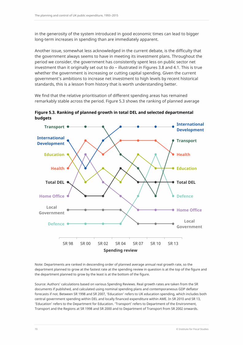
The planning and control of UK public expenditure, 1993−2015
70 © Institute for Fiscal Studies
in the generosity of the system introduced in good economic times can lead to bigger long-term increases in spending than are immediately apparent.
Another issue, somewhat less acknowledged in the current debate, is the difficulty that the government always seems to have in meeting its investment plans. Throughout the period we consider, the government has consistently spent less on public sector net investment than it originally set out to do – illustrated in Figures 3.8 and 4.1. This is true whether the government is increasing or cutting capital spending. Given the current government’s ambitions to increase net investment to high levels by recent historical standards, this is a lesson from history that is worth understanding better.
We find that the relative prioritisation of different spending areas has remained remarkably stable across the period. Figure 5.3 shows the ranking of planned average
Figure 5.3. Ranking of planned growth in total DEL and selected departmental budgets
Note: Departments are ranked in descending order of planned average annual real growth rate, so the department planned to grow at the fastest rate at the spending review in question is at the top of the figure and the department planned to grow by the least is at the bottom of the figure.
Source: Authors’ calculations based on various Spending Reviews. Real growth rates are taken from the SR documents if published, and calculated using nominal spending plans and contemporaneous GDP deflator forecasts if not. Between SR 1998 and SR 2007, ‘Education’ refers to UK education spending, which includes both central government spending within DEL and locally financed expenditure within AME. In SR 2010 and SR 13, ‘Education’ refers to the Department for Education. ‘Transport’ refers to Department of the Environment, Transport and the Regions at SR 1998 and SR 2000 and to Department of Transport from SR 2002 onwards.
Health
Health
Defence
Defence
Local Government
Local Government
Education
Education
Home Office
Home Office
Transport
Transport International Development
International Development
Total DEL Total DEL
SR 98 SR 00 SR 02 SR 04 SR 07 SR 10 SR 13 Spending review
Conclusion
© Institute for Fiscal Studies 71
annual real growth rates for total DEL and selected departments, at each spending review from 1998 to 2013. Spending on health and international development has been consistently prioritised throughout the period: expenditure on those areas was always planned to grow at a faster rate than overall DEL. This was also the case for spending on education and transport (with the exceptions of education at SR 2004 and transport at SR 2010). In contrast, budgets for defence and local government have tended to fare less well. It is particularly interesting that the prioritised departments are similar in times of rapid fiscal expansion in the early 2000s, comparatively tight settlements at SR 2007 and in times of austerity since 2010.
A final observation we would make is that historical quantitative analysis in this area – in particular, comparing spending out-turns and plans, and understanding the drivers of any differences – is remarkably difficult. There are a myriad of classification changes and inconsistencies in the data series published over the period we consider, and the contents of Treasury publications in the past have clearly been influenced by political considerations. However, the establishment of the Office for Budget Responsibility has made a huge difference to the transparency and clarity with which public spending figures (and other public finances data) are published. The OBR is a very welcome addition to the institutional structure, and any future analysis of the way governments have planned, managed and controlled public spending since 2010 will greatly benefit from its independently produced publications and commentary.
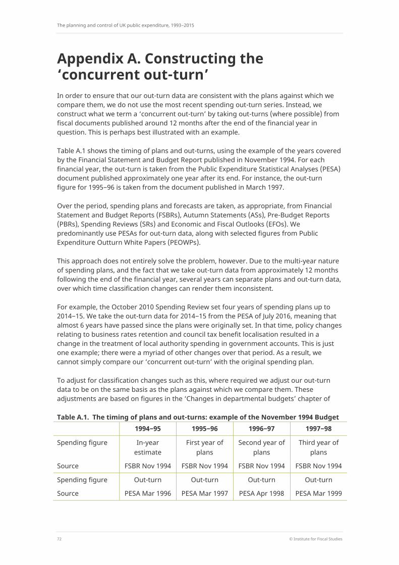
The planning and control of UK public expenditure, 1993−2015
72 © Institute for Fiscal Studies
Appendix A. Constructing the ‘concurrent out-turn’ In order to ensure that our out-turn data are consistent with the plans against which we compare them, we do not use the most recent spending out-turn series. Instead, we construct what we term a ‘concurrent out-turn’ by taking out-turns (where possible) from fiscal documents published around 12 months after the end of the financial year in question. This is perhaps best illustrated with an example.
Table A.1 shows the timing of plans and out-turns, using the example of the years covered by the Financial Statement and Budget Report published in November 1994. For each financial year, the out-turn is taken from the Public Expenditure Statistical Analyses (PESA) document published approximately one year after its end. For instance, the out-turn figure for 1995−96 is taken from the document published in March 1997.
Over the period, spending plans and forecasts are taken, as appropriate, from Financial Statement and Budget Reports (FSBRs), Autumn Statements (ASs), Pre-Budget Reports (PBRs), Spending Reviews (SRs) and Economic and Fiscal Outlooks (EFOs). We predominantly use PESAs for out-turn data, along with selected figures from Public Expenditure Outturn White Papers (PEOWPs).
This approach does not entirely solve the problem, however. Due to the multi-year nature of spending plans, and the fact that we take out-turn data from approximately 12 months following the end of the financial year, several years can separate plans and out-turn data, over which time classification changes can render them inconsistent.
For example, the October 2010 Spending Review set four years of spending plans up to 2014−15. We take the out-turn data for 2014−15 from the PESA of July 2016, meaning that almost 6 years have passed since the plans were originally set. In that time, policy changes relating to business rates retention and council tax benefit localisation resulted in a change in the treatment of local authority spending in government accounts. This is just one example; there were a myriad of other changes over that period. As a result, we cannot simply compare our ‘concurrent out-turn’ with the original spending plan.
To adjust for classification changes such as this, where required we adjust our out-turn data to be on the same basis as the plans against which we compare them. These adjustments are based on figures in the ‘Changes in departmental budgets’ chapter of
Table A.1. The timing of plans and out-turns: example of the November 1994 Budget 1994−95 1995−96 1996−97 1997−98 Spending figure In-year
estimate First year of
plans Second year of
plans Third year of
plans Source FSBR Nov 1994 FSBR Nov 1994 FSBR Nov 1994 FSBR Nov 1994 Spending figure Out-turn Out-turn Out-turn Out-turn Source PESA Mar 1996 PESA Mar 1997 PESA Apr 1998 PESA Mar 1999
Appendix A. Constructing the ‘concurrent out-turn’
© Institute for Fiscal Studies 73
PESA documents and, post 2010, figures published by the Office for Budget Responsibility. This means, however, that the out-turn figures underlying the graphs in this report may not match those in the official fiscal documents. Wherever we calculate the growth rate in an area of spending, we use a consistent spending series (i.e. not our concurrent out-turns). Whilst imperfect, this approach allows us to make meaningful comparisons between plans and out-turns, and to document changes in the predictability of public expenditure over the period.
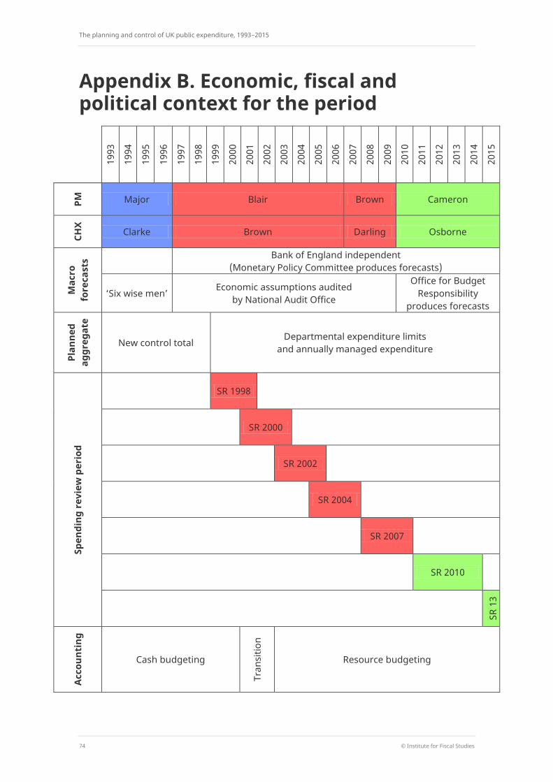
The planning and control of UK public expenditure, 1993−2015
74 © Institute for Fiscal Studies
Appendix B. Economic, fiscal and political context for the period
1993
1994
1995
1996
1997
1998
1999
2000
2001
2002
2003
2004
2005
2006
2007
2008
2009
2010
2011
2012
2013
2014
2015
PM
Major Blair Brown Cameron
CHX
Clarke Brown Darling Osborne
Mac
ro
fore
cast
s Bank of England independent (Monetary Policy Committee produces forecasts)
‘Six wise men’ Economic assumptions audited by National Audit Office
Office for Budget Responsibility
produces forecasts
Plan
ned
aggr
egat
e
New control total Departmental expenditure limits and annually managed expenditure
Spen
ding
rev
iew
per
iod
SR 1998
SR 2000
SR 2002
SR 2004
SR 2007
SR 2010
SR 1
3
Acco
unti
ng
Cash budgeting
Tran
sitio
n
Resource budgeting
Appendix B. Economic, fiscal and political context for the period
© Institute for Fiscal Studies 75
Fiscal rules and targets
NCT regime 1992–1995:
• Reduce general government expenditure (GGE) as a percentage of GDP.
1995−1997:
• Reduce GGE(X) to below 40% of GDP.
DEL/AME regime 1998–2008:
• The golden rule: over the economic cycle, the government will borrow only to invest and not to fund current spending.
• The sustainable investment rule: the ratio of net public sector debt to GDP will be kept below a ‘stable and prudent’ level, interpreted as 40% of GDP.
2008–2010:
• ‘Temporary operating rule’: set policies to improve the cyclically-adjusted current budget each year, once the economy emerges from the downturn, so it reaches balance and debt is falling as a proportion of GDP once the global shocks have worked their way through the economy in full.
2010:
• Fiscal Responsibility Act 2010: halve the overall budget deficit by 2013−14 from its 2009−10 level as a share of national income.
• Fiscal Responsibility Order 2010: reduce borrowing to no more than 5.5% of national income in 2013−14.
2010–2015
• The fiscal mandate: the structural current budget (that is, borrowing for non-investment spending, after adjusting for the economic cycle) must be forecast to be in balance or in surplus by the end of the rolling, five-year forecast horizon.
• The supplementary target: public sector net debt as a share of national income should be lower in 2015−16 than in 2014−15.
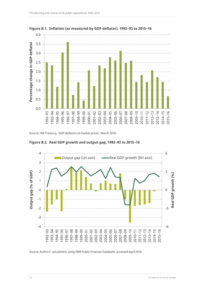
The planning and control of UK public expenditure, 1993−2015
76 © Institute for Fiscal Studies
Figure B.1. Inflation (as measured by GDP deflator), 1992−93 to 2015−16
Source: HM Treasury, ‘GDP deflators at market prices’, March 2018.
Figure B.2. Real GDP growth and output gap, 1992−93 to 2015−16
Source: Authors’ calculations using OBR Public Finances Databank, accessed April 2018.
0.0
0.5
1.0
1.5
2.0
2.5
3.0
3.5
4.0
1992
–93
1993
–94
1994
–95
1995
–96
1996
–97
1997
–98
1998
–99
1999
–00
2000
–01
2001
–02
2002
–03
2003
–04
2004
–05
2005
–06
2006
–07
2007
–08
2008
–09
2009
–10
2010
–11
2011
–12
2012
–13
2013
–14
2014
–15
2015
–16
Perc
enta
ge c
hang
e in
GD
P de
flato
r
-6
-3
0
3
6
-4
-3
-2
-1
0
1
2
3
4
1992
–93
1993
–94
1994
–95
1995
–96
1996
–97
1997
–98
1998
–99
1999
–00
2000
–01
2001
–02
2002
–03
2003
–04
2004
–05
2005
–06
2006
–07
2007
–08
2008
–09
2009
–10
2010
–11
2011
–12
2012
–13
2013
–14
2014
–15
2015
–16
Real
GD
P gr
owth
(%)
Out
put g
ap (%
of G
DP)
Output gap (LH axis) Real GDP growth (RH axis)
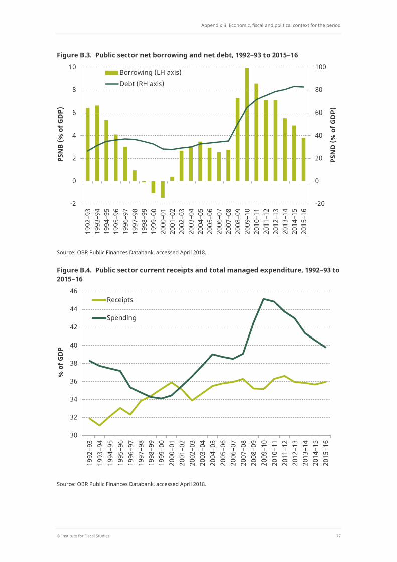
Appendix B. Economic, fiscal and political context for the period
© Institute for Fiscal Studies 77
Figure B.3. Public sector net borrowing and net debt, 1992−93 to 2015−16
Source: OBR Public Finances Databank, accessed April 2018.
Figure B.4. Public sector current receipts and total managed expenditure, 1992−93 to 2015−16
Source: OBR Public Finances Databank, accessed April 2018.
-20
0
20
40
60
80
100
-2
0
2
4
6
8
10
1992
–93
1993
–94
1994
–95
1995
–96
1996
–97
1997
–98
1998
–99
1999
–00
2000
–01
2001
–02
2002
–03
2003
–04
2004
–05
2005
–06
2006
–07
2007
–08
2008
–09
2009
–10
2010
–11
2011
–12
2012
–13
2013
–14
2014
–15
2015
–16
PSN
D (%
of G
DP)
PSN
B (%
of G
DP)
Borrowing (LH axis) Debt (RH axis)
30
32
34
36
38
40
42
44
46
1992
–93
1993
–94
1994
–95
1995
–96
1996
–97
1997
–98
1998
–99
1999
–00
2000
–01
2001
–02
2002
–03
2003
–04
2004
–05
2005
–06
2006
–07
2007
–08
2008
–09
2009
–10
2010
–11
2011
–12
2012
–13
2013
–14
2014
–15
2015
–16
% o
f GD
P
Receipts
Spending


