The phase diagram of the Haldane-Falicov-Kimball model · O diagrama de fases revelou tamb em uma...

The phase diagram of the Haldane-Falicov-Kimballmodel

Miguel de Jesus Mestre Goncalves

Thesis to obtain the Master of Science Degree in

Engineering Physics

Supervisors: Prof. Eduardo Filipe Vieira De Castro

Prof. Pedro Jose Goncalves Ribeiro

Examination Committee

Chairperson: Prof. Pedro Domingos Santos do Sacramento

Supervisor: Prof. Pedro Jose Goncalves Ribeiro

Members of the committee: Prof. Stefan Kirchner

September 2018

Acknowledgements

I would like to acknowledge:

• My advisers for their remarkable help and orientation along the development of this work and for the

inumerous discussions that provided an exceptional learning opportunity;

• CeFEMA and CSRC for the computer resources, that were essential for the attainment of the numerical

results in this work;

• Professor Rubem Mondaini for the fruitful discussions and help with some of the numerical aspects of

this work;

• Partial support from FCT-Portugal through Grant No. UID/CTM/04540/2013 and through the Inves-

tigador FCT contract IF/00347/2014;

• My family and Joana, for the outstanding support, essential to overcome the multiple challenges along

this work.

i

Resumo

Neste trabalho e obtido o diagrama de fases do modelo de Haldane-Falicov-Kimball a half-filling no plano da

interaccao-temperatura. Este modelo combina topologia, interaccoes e desordem a temperaturas finitas. Um

estudo numerico extensivo baseado nos metodos de campo medio variacional e Monte Carlo foi efectuado com

este proposito e complementado com um tratamento perturbativo analıtico. Como resultado central, foram

encontradas fases topologicas gapeadas e nao gapeadas induzidas pelo aumento da temperatura. Desordem

intrınseca - gerada por efeitos de temperatura - foi o ingrediente-chave para a percepcao deste fenomeno.

O diagrama de fases revelou tambem uma fase com ordem de carga nao gapeada, sugerindo a possibilidade

de esta estar associada a um limiar de mobilidade que separa regioes espectrais de estados localizados e

estendidos. As nossas descobertas sustentam a possibilidade da existencia de fases topologicas induzidas pelo

aumento da temperatura em sistemas com diferencas de massa elevadas entre especies fermionicas.

Palavras-chave: topologia, desordem, correlacoes fortes, modelo de Haldane, modelo de Falicov-Kimball

ii

Abstract

In this work we obtain the phase diagram of the Haldane-Falicov-Kimball model at half-filling in the

interaction-temperature plane, a model combining topology, interactions and disorder at finite tempera-

tures. An extensive numerical study based on the variational mean field and Monte Carlo methods was

carried out with this purpose and complemented with an analytical perturbative treatment. As a central

result, we found temperature-driven gapped and gapless topological insulating phases. Intrinsic - tempera-

ture generated - disorder, was the key ingredient for the understanding of such unexpected phenomena. The

phase diagram also unveiled an insulating charge ordered state with gapless excitations and the possibility for

this phase to be associated with a mobility edge separating spectral regions of localized and extended states.

Our findings support the existence of robust temperature-driven gapped and gapless topological insulating

phases in systems with a large mass unbalance in fermionic species.

Keywords: topology, disorder, strong correlations, Haldane model, Falicov-Kimball model

iii

Contents

1 Introduction 1

1.1 Topics of concern . . . . . . . . . . . . . . . . . . . . . . . . . . . . . . . . . . . . . . . . . . . 1

1.1.1 Phases and phase transitions . . . . . . . . . . . . . . . . . . . . . . . . . . . . . . . . 1

1.1.2 Strongly correlated systems . . . . . . . . . . . . . . . . . . . . . . . . . . . . . . . . . 2

1.1.3 Disordered systems and localization . . . . . . . . . . . . . . . . . . . . . . . . . . . . 4

1.1.4 Topological systems . . . . . . . . . . . . . . . . . . . . . . . . . . . . . . . . . . . . . 5

1.2 Objectives . . . . . . . . . . . . . . . . . . . . . . . . . . . . . . . . . . . . . . . . . . . . . . . 7

1.3 State of the art . . . . . . . . . . . . . . . . . . . . . . . . . . . . . . . . . . . . . . . . . . . . 8

1.3.1 Falicov-Kimball model . . . . . . . . . . . . . . . . . . . . . . . . . . . . . . . . . . . . 8

1.3.2 Haldane model . . . . . . . . . . . . . . . . . . . . . . . . . . . . . . . . . . . . . . . . 8

1.3.3 Topology, disorder and correlations at finite temperatures . . . . . . . . . . . . . . . . 9

1.4 Thesis outline . . . . . . . . . . . . . . . . . . . . . . . . . . . . . . . . . . . . . . . . . . . . . 11

2 Haldane-Falicov-Kimball model 12

2.1 Hamiltonian . . . . . . . . . . . . . . . . . . . . . . . . . . . . . . . . . . . . . . . . . . . . . . 12

2.2 Particle-hole symmetry . . . . . . . . . . . . . . . . . . . . . . . . . . . . . . . . . . . . . . . . 13

2.3 Half-filling . . . . . . . . . . . . . . . . . . . . . . . . . . . . . . . . . . . . . . . . . . . . . . . 14

2.4 Partition function . . . . . . . . . . . . . . . . . . . . . . . . . . . . . . . . . . . . . . . . . . . 14

3 Methods 16

3.1 Variational mean field method . . . . . . . . . . . . . . . . . . . . . . . . . . . . . . . . . . . . 16

3.2 Monte Carlo Metropolis Hastings . . . . . . . . . . . . . . . . . . . . . . . . . . . . . . . . . . 18

3.2.1 Binder cumulants . . . . . . . . . . . . . . . . . . . . . . . . . . . . . . . . . . . . . . . 20

3.3 Methods for computing c-electron’s observables . . . . . . . . . . . . . . . . . . . . . . . . . . 21

3.3.1 Coupling matrix method to compute the Chern number . . . . . . . . . . . . . . . . . 21

3.3.2 Recursive method for computing the DOS . . . . . . . . . . . . . . . . . . . . . . . . . 26

3.3.3 Transfer Matrix Method (TMM) . . . . . . . . . . . . . . . . . . . . . . . . . . . . . . 29

3.3.4 Inverse participation ratio (IPR) . . . . . . . . . . . . . . . . . . . . . . . . . . . . . . 32

iv

3.3.5 Level spacing statistics (LSS) . . . . . . . . . . . . . . . . . . . . . . . . . . . . . . . . 33

4 Disordered Haldane model 35

4.1 Numerical results . . . . . . . . . . . . . . . . . . . . . . . . . . . . . . . . . . . . . . . . . . . 35

4.1.1 Topological phase diagram’s evolution . . . . . . . . . . . . . . . . . . . . . . . . . . . 36

4.1.2 Phase diagram in the (W, η) plane . . . . . . . . . . . . . . . . . . . . . . . . . . . . . 37

4.1.3 Phase diagram in the (V, η) plane . . . . . . . . . . . . . . . . . . . . . . . . . . . . . . 38

4.1.4 Gapped and gapless regions of the phase diagram . . . . . . . . . . . . . . . . . . . . . 39

4.2 Perturbative analysis for small disorder . . . . . . . . . . . . . . . . . . . . . . . . . . . . . . 41

4.2.1 Application of first order Born approximation to Haldane model . . . . . . . . . . . . 41

5 Variational mean field results 45

5.1 CDW phase transition . . . . . . . . . . . . . . . . . . . . . . . . . . . . . . . . . . . . . . . . 45

5.1.1 Procedure to obtain TCDW . . . . . . . . . . . . . . . . . . . . . . . . . . . . . . . . . 45

5.1.2 Phase diagram . . . . . . . . . . . . . . . . . . . . . . . . . . . . . . . . . . . . . . . . 46

5.2 Topological phase diagram . . . . . . . . . . . . . . . . . . . . . . . . . . . . . . . . . . . . . . 47

5.2.1 Phase diagram in the (U, δ) parameter space . . . . . . . . . . . . . . . . . . . . . . . 48

5.2.2 Localization properties . . . . . . . . . . . . . . . . . . . . . . . . . . . . . . . . . . . . 48

5.2.3 Phase diagram in the (U, T ) parameter space . . . . . . . . . . . . . . . . . . . . . . . 49

5.3 Complete phase diagram . . . . . . . . . . . . . . . . . . . . . . . . . . . . . . . . . . . . . . . 51

5.3.1 Phase diagram in the (U, δ) parameter space . . . . . . . . . . . . . . . . . . . . . . . 51

5.3.2 Complete phase diagram in the (U, T ) parameter space . . . . . . . . . . . . . . . . . 53

5.3.2.1 DOS for different regions of the phase diagram . . . . . . . . . . . . . . . . . 54

5.4 Finite temperature topological phases . . . . . . . . . . . . . . . . . . . . . . . . . . . . . . . 55

5.5 Final remarks . . . . . . . . . . . . . . . . . . . . . . . . . . . . . . . . . . . . . . . . . . . . . 56

6 Perturbation theory: Small and large U 57

6.1 Perturbation expansion of H(nf) . . . . . . . . . . . . . . . . . . . . . . . . . . . . . . . . . 57

6.2 Large U . . . . . . . . . . . . . . . . . . . . . . . . . . . . . . . . . . . . . . . . . . . . . . . . 58

6.2.1 Second order expansion . . . . . . . . . . . . . . . . . . . . . . . . . . . . . . . . . . . 58

6.2.2 Effective 2D Ising model . . . . . . . . . . . . . . . . . . . . . . . . . . . . . . . . . . . 60

6.2.2.1 Disordered phase for higher values of t2 . . . . . . . . . . . . . . . . . . . . . 61

6.3 Small U . . . . . . . . . . . . . . . . . . . . . . . . . . . . . . . . . . . . . . . . . . . . . . . . 62

6.3.1 Low energy Haldane Hamiltonian and Green’s function . . . . . . . . . . . . . . . . . 62

6.3.2 Second order expansion . . . . . . . . . . . . . . . . . . . . . . . . . . . . . . . . . . . 64

6.3.3 Effective 2D Ising model . . . . . . . . . . . . . . . . . . . . . . . . . . . . . . . . . . . 66

v

7 Monte Carlo results 68

7.1 CDW phase transition . . . . . . . . . . . . . . . . . . . . . . . . . . . . . . . . . . . . . . . . 68

7.2 Complete phase diagram . . . . . . . . . . . . . . . . . . . . . . . . . . . . . . . . . . . . . . . 69

7.3 Localization properties . . . . . . . . . . . . . . . . . . . . . . . . . . . . . . . . . . . . . . . . 72

7.4 Finite temperature topological phases . . . . . . . . . . . . . . . . . . . . . . . . . . . . . . . 73

8 Conclusion 75

A Cubic spline method 88

A.1 Description of the method . . . . . . . . . . . . . . . . . . . . . . . . . . . . . . . . . . . . . . 88

A.2 Error propagation . . . . . . . . . . . . . . . . . . . . . . . . . . . . . . . . . . . . . . . . . . 89

A.2.1 Error in polynomials . . . . . . . . . . . . . . . . . . . . . . . . . . . . . . . . . . . . . 89

A.2.2 Error in x coordinate . . . . . . . . . . . . . . . . . . . . . . . . . . . . . . . . . . . . 89

A.2.3 Error in intersection between polynomials . . . . . . . . . . . . . . . . . . . . . . . . . 90

B Variational mean field for the HFKM - analytical approach 91

B.1 Effective Hamiltonian . . . . . . . . . . . . . . . . . . . . . . . . . . . . . . . . . . . . . . . . 91

B.1.1 Cross-check between analytical and numerical results . . . . . . . . . . . . . . . . . . . 93

B.2 Phase diagram . . . . . . . . . . . . . . . . . . . . . . . . . . . . . . . . . . . . . . . . . . . . 94

C Monte Carlo - Technical details 95

C.1 Errors and correlation times . . . . . . . . . . . . . . . . . . . . . . . . . . . . . . . . . . . . . 95

C.2 Numerical computation of correlation times . . . . . . . . . . . . . . . . . . . . . . . . . . . . 96

C.3 Jackknife method for computing errors . . . . . . . . . . . . . . . . . . . . . . . . . . . . . . . 97

D Connection between partition function and fermionic propagator through path integral

formalism 98

vi

List of Figures

1.1 I) Image taken from Ref. [4]. Example of CDW obtained with scanning tunneling microscopy

(STM) in single-layer NbSe2 on bilayer graphene (BLG) substrate. a, Top and side view

sketches of single-layer NbSe2, including the substrate; b, Large-scale STM image of NbSe2/BLG;

c-e, Atomically resolved STM images of single-layer NbSe2 for different temperatures. II)

Demonstration of the quantum Hall effect. Left: Landau levels with a Lorentzian DOS. EF

stands for Fermi energy. The occupied states are colored in red. Right: Hall conductivity

(ρxy) and longitudinal conductivity (ρxx) as a function of the magnetic field. The red dot on

the second-to-last plateau corresponds to the situation observed in the left figure, in which

only two Landau levels are filled. . . . . . . . . . . . . . . . . . . . . . . . . . . . . . . . . . . 3

1.2 a, Unit cell for the honeycomb lattice in the Haldane model. The parameter a corresponds

to the honeycomb lattice constant. The flow of fluxes φ is represented by the arrows: if the

electron hops in the direction of the arrow, the sign is positive, otherwise, it is negative. b,

Phase diagram of the Haldane model. . . . . . . . . . . . . . . . . . . . . . . . . . . . . . . . 9

1.3 Image taken from Ref. [78] showing the phase diagram of the 2D half-filled FKM on a square

lattice. U is the interaction strength and T the temperature. . . . . . . . . . . . . . . . . . . 11

2.1 Sketch of the HFKM. The large red particles correspond to f-electrons (localized) and the

green particles to c-electrons (itinerant). The Haldane fluxes φij = ±φ are represented by the

blue arrows. These fluxes are as defined in section 1.3.2 and the arrows indicate their sign: if

a c-electron hops in the direction of the arrow, the sign is positive, otherwise, it is negative.

There is an energy cost of U for a c-electron to hop into a site occupied with a f-electron due

to the on-site interactions between these fermionic species, also represented in the figure. . . . 12

3.1 a, Discretization of the Sθ surface boundary. The gray spots represent the discretized states,

separated by ∆lx or ∆ly. b, Discretization of the surface Sθ in small plaquettes that correspond

to loops in the discretized states. Notice that the sum of the fluxes in every plaquette yields

only the flux at the boundary (path λ(θ)) as the interior contributions cancel. This can be

seen in the example of the red and green plaquette. In this illustrative example, we have a

system with Nx = Ny = 5 plaquettes. . . . . . . . . . . . . . . . . . . . . . . . . . . . . . . . 22

vii

3.2 Representation of the zig-zag structures used to define the transfer matrices for the honeycomb

lattice. The full black line represents a given wire and each wire is labeled by index n. The

sites of a given wire are labeled by index i. The dashed green lines represent some examples

of the NNN hoppings of the Haldane model. Notice that these hoppings connect sites in the

same wire but also in neighboring chains. . . . . . . . . . . . . . . . . . . . . . . . . . . . . . 29

4.1 Evolution of the Haldane model’s phase diagram with Anderson disorder for a, W/t = 2; b,

W/t = 3.5; and c, W/t = 4. The black curves are the phase transition curves of the Haldane

model for null disorder. The results were obtained in units of t, for t2 = 0.1t. The results in

figures a) and b) were obtained for a 12 × 12 unit cell system while the ones in c) were for a

20× 20 system. 100 disorder configurations were used in total. . . . . . . . . . . . . . . . . . 36

4.2 Evolution of the Haldane model’s phase diagram with binary disorder for a, V/t = 2; b,

V/t = 2.4; and c, V/t = 2.75. The black curves are the phase transition curves of the Haldane

model for null disorder. The results were obtained in units of t, for t2 = 0.1t. The results in

figure a) were obtained for a 12× 12 unit cell system while the ones in figures b) and c) were

obtained for 20× 20 unit cell systems. . . . . . . . . . . . . . . . . . . . . . . . . . . . . . . . 36

4.3 Example of the Chern number’s curves obtained for different system sizes. For this example,

W/t = 1. . . . . . . . . . . . . . . . . . . . . . . . . . . . . . . . . . . . . . . . . . . . . . . . 37

4.4 a, Phase diagram of the Haldane model with Anderson disorder in the (W, η) plane for φ = π/2.

b, Phase diagram of the Haldane model with binary disorder in the (V, η) plane for φ = π/2.

The insets correspond to a zoom in the phase diagrams for small disorder. The thinner brown

curves below the numerical results in the insets correspond to the analytical results obtained

with the first order self-consistent Born approximation (see section 4.2). The dashed green

lines in b) correspond to the regions of the phase diagram for which the results of the TMM are

exemplified in Fig. 4.5. The errors associated with the intersection of the two cubic splines used

to compute the phase transition points are also shown. Points associated with the horizontal

and vertical error bars were respectively obtained by varying the disorder strength with fixed

η and vice-versa. . . . . . . . . . . . . . . . . . . . . . . . . . . . . . . . . . . . . . . . . . . . 38

4.5 Results of the TMM for large values of binary disorder. a, V/t = 2.5; b, V/t = 2.8. The

legend indicates the different values of M used. ΛM decreases with M except in the phase

transition points for which this quantity remains unchanged. This behaviour is the expected

for trivial and topological insulating phases. The single critical point obtained for V/t = 2.5

and the two critical points obtained for V/t = 2.8 are in accordance with the results obtained

for the Chern number in Fig. 4.4 and are marked with arrows. . . . . . . . . . . . . . . . . . . 39

viii

4.6 Gapped and gapless regions of the φ = π/2 phase diagrams in the (W, η) (a) and (V, η) (b)

planes. The computations were carried out for systems of 1000× 1000 unit cells. The system

was considered gapped whenever the DOS at the Fermi energy was below a threshold value of

0.1%× refDOS, where refDOS was chosen to be the inverse bandwidth of the non-disordered

system, that is, refDOS = 1/6t. . . . . . . . . . . . . . . . . . . . . . . . . . . . . . . . . . . . 39

4.7 Plots of the DOS for points A-E represented in the phase diagrams of a, Fig. 4.6a; b, Fig. 4.6b.

Systems of 1000× 1000 unit cells and a total of 20 disorder configurations were considered. . 40

4.8 Phase diagram computed with the zero order Born approximation for φ = π/2 , t2 = 0.1t and

Anderson disorder. . . . . . . . . . . . . . . . . . . . . . . . . . . . . . . . . . . . . . . . . . . 44

5.1 a, Free energy functional F for different temperatures and respective fits. b, Linear fit of the

b parameters obtained from the fits in a). The plot markers corresponding to points in b) are

the same as the ones used in the curves from which they were computed in a). In this example,

U = 5.5. . . . . . . . . . . . . . . . . . . . . . . . . . . . . . . . . . . . . . . . . . . . . . . . . 46

5.2 Phase diagram of the CDW phase for the HFKM. The honeycomb unit cell inside the CDW

phase represents the type of charge order present: the larger sites correspond to occupied

sites, demonstrating one of the two maximally ordered configurations, for which only one

sublattice is occupied. The inset shows a zoomed view of the small U results together with a

TCDW(U) ∝ U2 curve fitted to these data points. . . . . . . . . . . . . . . . . . . . . . . . . 47

5.3 a, Example of Chern number curves used to compute δCh. In this example, U = 1.789.

b, Phase diagram in the (U, δ) parameter space. The filled red region corresponds to the

topological phase (C = 1) while the unfilled region corresponds to the trivial phase (C = 0). . 48

5.5 Steps to obtain TCh(δCh). a, Free energy curves used to obtain the order parameter δ for

different temperatures T . b, Interpolation of the δ(T ) points obtained in figure a) in order to

find TCh. For this example, U = 1.114. . . . . . . . . . . . . . . . . . . . . . . . . . . . . . . 49

5.4 Results of the TMM for a, U = 2.25 and b, U = 2.5 for varying δ, at the Fermi energy.

The legend indicates the different values used for the transverse number of unit cells M in

the numerical computations. The arrows indicate the bulk extended states, associated with a

constant ΛM for different transverse sizes. . . . . . . . . . . . . . . . . . . . . . . . . . . . . 49

5.6 Topological phase diagram in the (U, T ) parameter space together with the CDW phase. The

blue and red curves bound respectively the CDW and topological phases. The region of

coexistence of the two phases is labeled as “coex.”. . . . . . . . . . . . . . . . . . . . . . . . . 50

5.7 Gapped and gapless regions of the HFKM in the (U, δ) parameter space. The description of

the different phases is provided in the text. . . . . . . . . . . . . . . . . . . . . . . . . . . . . 52

ix

5.8 Mean field phase diagram of the HFKM in the interaction strength (U) - temperature (T ) plane.

The blue curve bounds the charge density wave phase (CDW) phase and was already shown

in Fig. 5.2. The different phases follow: outside the CDW phase, topological insulator (TI) for

small U , gapless topological insulator (GTI) and gapless insulator (GI) for intermediary U , and

Mott-like insulating phase (MI) for large U . Inside the CDW phase, c-electron’s phases with

similar features as their high temperature counterparts were found and the suffix “/CDW”

was added. . . . . . . . . . . . . . . . . . . . . . . . . . . . . . . . . . . . . . . . . . . . . . . 53

5.9 Points in the phase diagram for which the DOS is shown in Figs. 5.10-5.12. . . . . . . . . . . 54

5.10 DOS for points Ai (a) and Bi (b) in the phase diagram, marked in Fig. 5.9. . . . . . . . . . . 54

5.11 DOS for points Ci (a) and Di (b) in the phase diagram, marked in Fig. 5.9. . . . . . . . . . 54

5.12 DOS for points Ei in the phase diagram, marked in Fig. 5.9. . . . . . . . . . . . . . . . . . . . 55

5.13 TMM results for U/t = 2 and U/t = 2.25 within the disordered phase. The legend shows the

different used values of the transverse system size M . The red arrows point at the extended

states signaled by a constant ΛM as a function of M . . . . . . . . . . . . . . . . . . . . . . . . 56

6.1 Comparison between the large U results obtained with perturbation theory and the numerical

results obtained with the variational mean field method for the CDW phase transition curve,

TCDW(U). . . . . . . . . . . . . . . . . . . . . . . . . . . . . . . . . . . . . . . . . . . . . . . 61

6.2 a, Checkerboard (CB) and collinear striped (CS I and CS II) configurations. b, Difference

between the energy of the checkerboard (ECB) and collinear striped (ECS) configurations for

different interaction strengths U . . . . . . . . . . . . . . . . . . . . . . . . . . . . . . . . . . . 62

6.3 a, Coupling coefficients Jij as a function of distance R which is in units of the lattice constant

a. In blue we show the couplings for sites in the same sublattice, either being sublattice A

(JAA) or B (JBB), and in red, we show couplings between different sublattices (JAB). The

Green dashed lines mark the distance R corresponding to first (R = 1), second (R =√

3) and

third (R = 2) nearest neighbors. b, Comparison between the analytical results obtained with

perturbation theory for small U and the numerical results obtained with mean field. . . . . . 66

7.1 Phase diagram of the CDW phase of the HFKM obtained with the MC method together with

the MF and PT results. The inset shows an example of the usage of the Binder cumulant

method to compute the critical temperature TCDW. . . . . . . . . . . . . . . . . . . . . . . . 69

7.2 Phase diagram of the HFKM in the interaction U - temperature T plane obtained with the MF

(a) and MC (b) methods. The different phases follow: outside the charge density wave phase

(CDW), topological insulator (TI) for small U , gapless topological insulator (GTI) and gapless

insulator (GI) for intermediary U and Mott-like insulating phase (MI) for large U . Inside the

CDW phase, phases with similar features as their high temperature counterparts were found

and the suffix “/CDW” was added. . . . . . . . . . . . . . . . . . . . . . . . . . . . . . . . . . 70

x

7.3 a - c, Density of states for different points in the phase diagram: MI/CDW-(U, T ) = (2.5, 0.045),

GI/CDW-(2.5, 0.085), TI-(1, 0.2), GTI-(2, 0.2), GI-(4, 0.2) and MI-(5, 0.2). The DOS plots are

shown with a Lorentzian broadening of width 0.01 and were obtained for L = 16. d, Finite

size scaling of the DOS at E = 0 for the point (2.5, 0.085) used in figure b. V0 corresponds to

the volume of the smallest used system (with L = 8). The DOS(E = 0) was computed in an

energy window corresponding to 1% of the full bandwidth for the L = 8 system. This window

was reduced proportionally to the system size for larger systems. . . . . . . . . . . . . . . . . 71

7.4 Chern number computed through averages on Monte Carlo configurations of f-electrons for

different system sizes, for fixed U (a) and T (b). These curves were used to obtain the

topological phase transition curve in Fig. 7.2. . . . . . . . . . . . . . . . . . . . . . . . . . . . 71

7.5 a, Variance of the LSS distributions obtained for different energies in the GI (GTI) phase for

(U, T ) = (2, 0.1) ( = (3.5, 0.2) ) and L = 14. The thick red line corresponds to σ2/〈s〉2 = 0.178

which is the variance of the Wigner distribution associated to extended states. The two

extended states existing in the GTI phase are marked with arrows. b (e), Finite size scaling

of the IPR with the system’s volume V for the energies marked with the arrows in figure c

(d), that shows the IPR for different sizes in the GI/CDW (GI) phase for (U, T ) = (2.5, 0.085)

(= (3.5, 0.2) ). The IPR shown in figure c (d) for negative (positive) energies is symmetric

in E. The red dashed lines shown in figures b,e have a unit slope and indicate the scaling

IPR ∼ V −1. The colors of the arrows that select specific energies in figure c (d) match the

corresponding scaling curves in figure b (e). . . . . . . . . . . . . . . . . . . . . . . . . . . . . 73

7.6 a, Variance of the level spacing distributions obtained for (U, T ) = (2, 0.1) for different system

sizes. b, Variance of the level spacing distributions and DOS for (U, T ) = (1.5, 0.06), a point

inside the TI phase and very close to the topological phase transition curve. The arrows

indicate the position of the extended states. The red line indicates the variance expected for

extended states in the unitary class, σ2/〈s〉2 = 0.178. . . . . . . . . . . . . . . . . . . . . . . 73

B.1 Cross check between analytical and numerical results for T = 0 and the configuration corre-

sponding to every sites of types A and B respectively occupied and empty. . . . . . . . . . . 94

B.2 Phase diagram of the HFKM obtained through the variational mean field method under the

approximation in expression B.1. . . . . . . . . . . . . . . . . . . . . . . . . . . . . . . . . . . 94

xi

Glossary

HFKM Haldane-Falicov-Kimball model

FKM Falicov-Kimball model

CDW Charge density wave

TMM Transfer matrix method

MF Mean field

MC Monte Carlo

PH Particle-hole

DOS Density of states

NN Nearest neighbors

NNN Next nearest neighbors

NNNN Next-to-next nearest neighbors

TAI Topological Anderson insulator

xii

Chapter 1

Introduction

Strong correlations, disorder and topology are three central topics in Condensed Matter Physics. Although

several important studies regarding each topic have been carried on, few have considered the interplay between

them at finite temperatures. With the rising effort to find new topological materials such combined approach

ought to be taken in order to understand how topology can be stabilized and, more importantly, if new

topological phases with interacting counterparts can be found. To understand the aim of the thesis project,

it is first important to introduce each of these areas and understand why they are so important.

1.1 Topics of concern

1.1.1 Phases and phase transitions

The general public often associates phases with the states of matter that we see around us: solids, liquids

and gases. In fact, the concept of phases is more general and rigorously we can say that two states of matter

are in the same phase if we can transform one into another continuously without abrupt modifications in

their properties, with the manipulation of the system’s parameters such as temperature and pressure. With

this definition, many other different phases can be enumerated: metal/insulator, ferromagnet/paramagnet,...

Typically we can have ordered and disordered phases depending on the temperature of our system. For

large temperatures, a large number of configurations is accessible and therefore the system is in a disordered

phase. If we decrease the temperature to some critical value, we can have a phase transition into an ordered

phase. These phases are defined by an order parameter that vanishes in the disordered phase and is finite in

the ordered phase. There are many examples of order such as magnetic and charge ordering. A ferromagnet

is a representative example of magnetic ordering. For this system, the order parameter is the total magnetic

moment of the system, that is, the total magnetization. For large temperatures, the magnetic moments

associated to different atoms are distributed in random directions, which means that the total magnetization

vanishes and the system becomes a paramagnet. However, below some critical temperature, these moments

1

start to align in a given direction and the system acquires a non-zero magnetization, thus becoming a

ferromagnet.

The phase transitions between ordered and disordered phases are described by Landau theory. This the-

ory explains the existence of first and second order phase transitions, which are respectively associated to a

discontinuous and continuous change of the order parameter in the phase transition. Furthermore, it provides

a framework to analyse second order phase transitions in terms of the symmetries and dimensionality of the

system [1]. Phase transitions from disordered to ordered phases are associated to a spontaneous symme-

try breaking. For instance, for the ferromagnet/paramagnet example, the magnetization has no preferred

direction in the paramagnetic phase, and so has rotational symmetry (SO(3)), but when we enter the ferro-

magnetic phase, the magnetization assumes a preferred direction, thus leading to a spontaneous symmetry

breaking of this symmetry.

There are, however, some phases which cannot be distinguished by any local order parameter. Rather,

these phases depend on the topology of the eigenstates of our system. They are called topological phases

and give rise to a new type of materials which are insulators in bulk and conductors at the surface: the

topological insulators. We will come back to topological systems below.

Metals and insulators are other examples of phases as they respectively conduct and do not conduct electric

current. These systems can be described with band theory [1] which is an approximation of the quantum

state of a solid built with single electron states in a periodic lattice of atoms or molecules. With this theory,

one can easily distinguish metals from insulators by obtaining the energy bands (range of energies that an

electron can have) and band gaps. However, it no longer holds if we have interactions as the description

with single particle states is insufficient. This is also the case of disordered systems, in which translational

invariance is broken and we cannot identify the wave vector as a good quantum number in the sense that we no

longer identify the eigenstates with it. Although with these two additional ingredients we still have insulators

with a gapped energy spectrum - Mott insulators - which are interaction-driven, we can have disorder-driven

insulators that do not have a gapped spectrum but are nonetheless insulators due to the localization of their

eigenstates - Anderson insulators. The metal/insulator distinction then needs to be analysed with a different

perspective based on the identification of the eigenstates of the system as localized or extended.

1.1.2 Strongly correlated systems

There are some systems in which electron-electron interactions cannot be neglected and the many body effects

dominate the most important inherent physics. Strong interactions are heavily related to large electron

correlations. Correlations are often associated with the appearence of ordered phases at sufficiently low

temperatures. For such low temperatures, the interactions dominate over the kinetic energy and therefore

the electron arrangement becomes important in order for the energy to be minimized. It is important to

notice however that the system’s dimensionality also plays an important role in the existence of ordered

phases. For low dimensions it can happen that we do not have any ordered phase as the quantum and

2

ρxx

ρxy (h/e2)(arb. units)ρxx

a

3.44Å

III

Energ

y

EF

DOS Magnetic Field (T)

Top view Side view

Nb

Se

C

b

c

d

e

Figure 1.1: I) Image taken from Ref. [4]. Example of CDW obtained with scanning tunneling microscopy(STM) in single-layer NbSe2 on bilayer graphene (BLG) substrate. a, Top and side view sketches of single-layer NbSe2, including the substrate; b, Large-scale STM image of NbSe2/BLG; c-e, Atomically resolvedSTM images of single-layer NbSe2 for different temperatures. II) Demonstration of the quantum Hall effect.Left: Landau levels with a Lorentzian DOS. EF stands for Fermi energy. The occupied states are colored inred. Right: Hall conductivity (ρxy) and longitudinal conductivity (ρxx) as a function of the magnetic field.The red dot on the second-to-last plateau corresponds to the situation observed in the left figure, in whichonly two Landau levels are filled.

thermal fluctuations overcome the correlations responsible for the emergence of ordering.

As a simple example of an ordered phase driven by correlations, we can take a 2D ensemble of equally

spaced atoms and a number of electrons half the number of atoms, such that the Coulomb interaction between

electrons dominates the most relevant physics. In this case, the configuration that minimizes the energy is

one in which every other site is occupied. This is an example of charge ordering and can in fact be seen

as a large amplitude charge density wave (CDW) [2]. In this case the charge-ordered state does not have

the full translational symmetry of the chain and therefore, as for the ferromagnet’s example of magnetic

ordering mentioned in the previous section, we have symmetry breaking. This is in fact quite general and one

important effect of the electron-electron interactions: the appearence of ground states with less symmetries

than the Hamiltonian due to spontaneous symmetry breaking.

As some examples of materials that manifest important correlation effects, we have transition metals,

rare earth elements and actinides. An example of a measured CDW (charge ordered phase) in a single two-

dimensional (2D) layer of NbSe2 is shown in Fig. 1.1(I). For the highest temperature case 1.1(Ic) we can see

that the undistorted crystal structure shown in Fig. 1.1(Ia) is still observed. For the smallest temperature case

a CDW superlattice is observed in which the ions are arranged in a different way leading to an electron density

modulated in space. In fact this superlattice has an unit cell 3× 3 larger than the one from the undistorted

crystal. This clearly shows a real example in which the initial translational symmetry is spontaneously

broken.

Strong correlations can also drive metal-insulator transitions and the resulting interaction-driven insula-

tors are called Mott insulators, as stated before [3].

3

1.1.3 Disordered systems and localization

To understand disordered systems it is important to introduce the concepts of localized and extended states.

When we have an eletron moving in a periodic infinite lattice, Bloch’s theorem states that its wavefunctions

are in the form of Bloch waves [1]. When we add disorder (with impurities, lattice distortions,...), Bloch

waves are no longer the eigenstates of the system due to the loss of translational symmetry. We can use a

semiclassical picture to understand that when this happens, the electron scattering in these irregularities will

enable the change between Bloch states which acquire a lifetime τ , within an energy scale which is inversely

proportional to this time scale. In this picture, the conductivity is proportional to τ (Drude formula) [5]. A

finite τ means we have extended states, which are associated to a non-null conductivity, and are therefore

metallic states. On the other hand, if τ = 0, the eigenstates are localized.

A localized state can be defined as having a probability amplitude exponentially decreasing in a region

around some central position r′. This implies that the corresponding wavefunction can be written as

Ψ(r) = f(r)e−|r−r′|/ξ , (1.1)

where ξ is defined as the localization length.

In 1958 P.W. Anderson suggested that it was possible to obtain localization in a lattice potential if the

degree of randomness (and therefore disorder) in this potential was sufficiently large [6]. Therefore, a system

which is metallic can turn into an insulator with the introduction of disorder. This type of insulator is now

known as the Anderson insulator. In 1D it was discovered shortly afterwards (Mott and W. D. Twose [7])

that any degree of disorder would lead to localization. In larger dimensions, localization was a much harder

problem to solve. In 1979, Abrahams, Anderson, Licciardello and Ramakrishnan published an article in which

they introduced the one parameter scaling theory of localization [8]. This study was very important as it

provided an analysis on the localization effects for higher dimensions. It showed that for two dimensions, we

would still always have localization and therefore no metallic regime would be present. For three dimensions,

however, it showed that there was a well defined energy separating extended from localized states, the so

called mobility edge [9].

It is, however, important to notice that all the results from the previous paragraph were valid for the

orthogonal symmetry class which encompasses systems that are invariant under spin rotation and time

reversal (with T 2 = 1, T being the time-reversal operator). This symmetry class is one of the three belonging

to the original Wigner-Dyson classification [10]. The other two are the sympletic class (time reversal symmetry

with T 2 = −1) and the unitary class (time reversal symmetry broken, for instance due to the presence of

a magnetic field). In 2D, a well defined energy separating extended from localized states exists for the first

class and extended states can appear at specific energies for the second. The Wigner-Dyson classification was

later extended to include topological features leading to a ”tenfold way” with the addition of chiral classes

[11]. These considerations already show that disorder plays a very important role in 2D systems, the ones

4

with which we will be concerned in this thesis.

1.1.4 Topological systems

In the previous sections, we have seen that we can have systems with ordered and disordered phases char-

acterized by an order parameter and that the transition between these phases occurs with a spontaneous

symmetry breaking. This description corresponds to the phenomenological Landau theory. This theory has,

however, some limitations, the major one being the fact that it considers a local order parameter. In the

decade of 1970, the concept of phases of matter without a local order parameter was first suggested and

explained by Kosterlitz and Thouless [12]. These findings first established the role of topology in physics.

Topology is the branch of mathematics that studies quantities which are invariant under continuous

deformations. These quantities are called topological invariants. If we take for instance a sphere with n

holes, n is a topological invariant as we cannot continuously deform this sphere into another with a different

number of holes. Topological invariants are very important as they are what distinguishes a topological and

a trivial phase.

The first examples of topological phases realized experimentally involved strong magnetic fields. Some

states of matter composed by free fermions, once considered topologically trivial, showed interesting topo-

logical properties such as gapless edge states, that is, conducting states occurring only at the surface of the

bulk insulating material. The materials that express these features are now called topological insulators.

The first experimental evidence of such phenomena was the integer quantum Hall effect. To explain

the quantum effect, we must first understand the classical Hall effect [13]. Applying a magnetic field to

a conductor perpendicular to the current flow gives rise to a voltage perpendicular both to the magnetic

field and current directions - the Hall voltage VH . The Hall resistance can then be defined as ρxy = VH/I.

Classically, ρxy was shown to be proportional to the magnetic field B. However, in 1980, Klaus Von Klitzing

measured the Hall effect for a small temperature (T = 50mK) in samples with electrons confined to move

in two dimensions only [14]. He found that for small magnetic fields the linear behaviour of ρxy with B was

observed. However, for large magnetic fields, something odd happened: the Hall resistance had plateaus that

could be described with great precision by

ρxy =h

e2

1

n, n integer . (1.2)

This effect is purely quantum and could not be explained within a classical approach. For large magnetic

fields, the atomic potential can be neglected and the problem reduces to the motion of electrons confined to

a plane in an uniform charge background and subjected to a large magnetic field. This problem had already

been solved by Landau in 1930 [15]. He obtained that the energy spectrum of the system was quantized

with energies En = ~ωc(n + 1/2), the so called Landau levels, where ωc = eB/m. The degeneracy of these

levels was shown to be proportional to the magnetic field and therefore, for large enough magnetic fields

5

each Landau level can have a large electron occupation. If the total number of electrons Ne in the system

is multiple of the number of states per Landau level NB , then it is natural that we have a quantized Hall

conductivity given by σxy = 1/ρxy = e2/hn, where n = Ne/NB . But this does not explain the plateaus.

In fact, the explanation is really interesting and motivates the relevance of this example for this work -

it sits on disorder effects. The consequence of the presence of disorder is the broadening of the density of

states (DOS) around the Landau levels into a Lorentzian lineshape as shown in Fig. 1.1(II). If we remember

our definitions of the symmetry classes in section 1.1.3, this system belongs to the unitary symmetry class as

time reversal symmetry is broken due to the presence of a magnetic field. The consequence is that extended

states can remain at particular energies which, in this case, are located in the unperturbed Landau levels.

All other states are localized. This provides an answer to why we should observe the plateau: the jumps in

the Hall conductivity occur when the Fermi level crosses the unperturbed Landau levels. When the states

existing around these levels are filled, no change in the Hall conductivity should be noticed as those states

are localized. It is interesting to see how the first experimental emergence of topological effects had already

an interplay with disorder effects.

David Thouless and his collaborators further showed that the Hall conductivity σxy = ρ−1xy in two-

dimensional systems with periodic potentials should indeed be quantized - σxyh/e2 is a topological invariant

now known as the Chern number [16]. At this point, mathematical details are unavoidable to understand

what this topological invariant really is, and we next define a very important concept behind it: the Berry

phase.

To define the Berry phase, we introduce a general Hamiltonian H(R) that varies with some parameters

R and has instantaneous eigenstates |n(R)〉 obtained by diagonalizing H(R) at each value of R. The Berry

phase can then be defined as

γn = i

∫An(R) · dR , (1.3)

where

An(R) = 〈n(R)| ∇R |n(R)〉 (1.4)

is the Berry connection and the integration is performed along some path C. The Berry connection is gauge

dependent and therefore if we make a gauge transformation in the eigenstates |n(R)〉 → eiξ(R) |n(R)〉, it

transforms as An(R)→ An(R)−∇Rξ(R) and the Berry phase is therefore changed by ξ(R(0))− ξ(R(T ))

with R(0) and R(T ) being, respectively, initial and final points in path C. Before Berry, this phase was

considered unimportant as we can always choose a suitable ξ(R) in such a way that it is canceled. However,

Berry in 1984 noticed that this was not the case if a closed path was considered [17]. In this case, in order for

our eigenstate basis to be single-valued, the condition |n(R(0))〉 = |n(R(T ))〉 must be verified. This means

that ξ(R(0))− ξ(R(T )) = 2πn and so the Berry phase can only be changed by multiples of 2π, becoming a

6

gauge invariant quantity.

At this point, we introduce another quantity of big interest - the Berry curvature. Assuming that the system

is periodic in R, it can be defined in terms of the Berry connection as

∫CAn(R) · dR =

∫S

Ωn(R) · dS , (1.5)

where Ωn(R) = ∇R ×An(R) is the Berry curvature and surface S is the system’s unit cell. This is a very

important quantity because it is gauge invariant and is essential for understanding a variety of electronic

properties [18].

A topological invariant can be defined in terms of the Berry curvature as

C =1

2π

∫S

Ω(R) · dS . (1.6)

This invariant is called the Chern number. When it does not vanish, the system has non-trivial topology

and therefore, it is on a topological phase. What David Thouless and his collaborators showed was that

the Hall conductivity σxy in a two dimensional system with a periodic potential could be identified as the

topological invariant C [16].

In 1988, Duncan Haldane proposed a model of a topological insulator in a honeycomb lattice that unveiled

topological phases without the presence of an external magnetic field [19]. This is what is now known as

the Haldane model and is a pioneer example of the so called Chern insulators which are two dimensional

topological insulators that break time-reversal symmetry and exist for zero net magnetic field. In 2013, this

phase of matter was experimentally detected in thin films of Cr-doped (BiSb)2Te3 [20].

1.2 Objectives

The aim of the thesis project is to obtain new states of matter induced by the interplay between strong

correlations and topology in an intrisically disordered system, at finite temperatures. To do that, we study a

model already possessing all these features that consists of adding Falicov-Kimball interactions to the Haldane

model. The Falicov-Kimball model represents a type of interactive systems for which disorder-like effects were

recently shown to play a very important role. On the other hand, the Haldane model is representative of a

topological Chern insulator. The combination of the two models is our object of study and is labeled the

Haldane-Falicov-Kimball model (HFKM).

To attain the general goal stated, below we have divided the workplan into particular objectives:

• Learn and implement numerical methods to characterize localized and extended states, to compute the

Chern number and to obtain the system’s energy spectrum;

• Study the disordered Haldane model (high temperature limit of the HFKM);

7

• Use the variational mean field method to obtain the phase diagram of the HFKM in the interaction

strength/temperature parameter space;

• Use perturbation theory to study the small and large interaction strength limits;

• Implement a Monte Carlo algorithm to cross-check the mean field and perturbation theory results.

1.3 State of the art

1.3.1 Falicov-Kimball model

The Falicov-Kimball model (FKM) was introduced in 1969 with the objective of describing metal-insulator

transitions in rare-earths and transition metals [21]. It is one of the simplest models involving strong electron

correlations and a limiting case of the Hubbard model [22] in which the dynamics of one of the fermionic

species is neglected.

The FKM considers a species composed of itinerant electrons that can move in a lattice and another of

fixed electrons. The fixed electrons can be interpreted to be localized and interact with the itinerant electrons

through Coulomb repulsion which is considered only on-site.

The second quantized Hamiltonian is

HFK = −t∑〈ij〉

c†i cj −∑i

(µcc†i ci + µfnf,i) + U

∑i

c†i cinf,i , (1.7)

where operators ci and fi are respectively associated with itinerant and localized electrons. c†i creates an

itinerant electron at site i and nf,i = f†i fi is the density of f electrons at site i. The first term is the

kinetic energy of the itinerant electrons in which the sum is performed for nearest neighbor sites, with t

being the hopping integral for nearest neighbors. The second term represents the on-site energies, where µ

is the chemical potential and finally the last term is the Falicov-Kimball interaction that has strength U and

represents the local site Coulomb interaction between itinerant an localized electrons.

This model has important features that allow for the study on the interplay between disorder and strong

correlations. nf,i commutes with the Hamiltonian and the averaging on the f-electron configurations according

with the total partition function has the effect of a disorder-like potential to the itinerant electrons.

1.3.2 Haldane model

The Haldane model was proposed by Duncan Haldane in 1988 as a toy model with topological phases for

a zero net magnetic field in a two-dimensional system. It is a model in a honeycomb lattice corresponding

to the interpenetration of two different triangular lattices of sites A and B. It considers, additionally to the

kinetic energy term for hoppings between first neighbors (first term in HFK), a staggered potential η which

is +η in atoms A and −η in atoms B and second neighbor complex hoppings of the type t2eiφij . In the latter,

8

- π - π2

0 π2

π- 3 3

0

3 3

ϕ

η/t2

C=-1 C=

C=0

a b

+1a

Figure 1.2: a, Unit cell for the honeycomb lattice in the Haldane model. The parameter a corresponds tothe honeycomb lattice constant. The flow of fluxes φ is represented by the arrows: if the electron hops in thedirection of the arrow, the sign is positive, otherwise, it is negative. b, Phase diagram of the Haldane model.

φij = ±φ ∈] − π, π], and the sign depends on the arrows shown in Fig. 1.2a along with the unit cell for the

honeycomb lattice - if the electron hops in the direction of the arrow it is positive, otherwise, it is negative.

These are really fluxes of an implicitly imposed magnetic flux density. The interesting point is that these

fluxes were built in such a way that the total flux in the unit cell was null.

The staggered potential η breaks inversion symmetry while the fluxes φ break time-reversal symmetry.

These symmetry breakings open a gap in the normal graphene spectrum (in which η = t2 = 0) [23] and for

some parameters, it is possible for the resulting insulator to be in fact a topological insulator, as shown in

the phase diagram from Fig. 1.2b, where we can see two topological phases - the ones with non-zero Chern

number. The system is gapped for every point in the phase diagram except at the topological phase transition

curves for which the two energy bands in momentum space touch at the graphene’s Dirac points [23] with a

linear dispersion.

The Haldane model adds two additional terms to HFK . These are:

HH = t2∑〈〈i,j〉〉

e−iφijc†i cj +H.c.+ η∑i

ζic†i ci , (1.8)

where ci = ci,A, ci,B , ζi = ±1 respectively for sites of type A and B and the sum in the first term is between

second nearest neighbor sites.

1.3.3 Topology, disorder and correlations at finite temperatures

Recently, the influence of disorder, interactions and finite temperatures on topological phases of matter has

attracted a large theoretical interest in order to better understand the role of topology in real-world materials.

Strong interactions were shown to suppress topological phases when magnetic order was induced both for

Hubbard-like [24–33] and spinless nearest-neighbor (NN) interactions [34]. Magnetic ordering was also found

to be possible to coexist with topological phases to form antiferromagnetic topological insulating phases [35–

9

38]. Some mean field studies showed that interactions could also induce a topological phase when imposed in a

trivial band model, forming the so called topological Mott insulator [39–46], that exists in the strong-coupling

regime. The existence of this phase outside the mean field scope has been questioned multiple times [47–50]

and a significant amount of attention has turned to weak coupling interaction-driven topological insulating

phases in 2D systems with quadratic band crossing points [51–57].

The influence of correlations at finite temperatures on TI has also already been studied [58–61]. Although

thermal fluctuations are responsible for the destruction of topological order when large enough [62], they can

also drive different types of topological phases [59, 63].

Among the studies on the influence of disorder in TI, it has been found that for 2D models belonging to

the unitary class (for which time-reversal symmetry is broken) such as the Haldane model, disorder effects

localize every eigenstate except two bulk extended states that carry opposite Chern numbers in the topological

phase [64, 65]. The merging of these states was shown to be associated with the destruction of the topological

phase for a sufficiently large disorder strength. Disorder studies on topology also unveiled a new class of TI

for which a disorder-induced topological phase transition into a topological phase is possible - topological

Anderson insulators (TAI) [66–70].

Regarding the models of concern, in [71–73] it was suggested the usage of a Monte Carlo (MC) method

based on the Metropolis Hasting algorithm in simulations of the FKM on a lattice. The usage of this method

takes into account the fact that nf,i is a conserved quantity in the FKM and therefore the partition function

of the model can be written as a summation in the non-interacting contributions from each configuration of

localized eletrons. The method is then used with a sampling of the configurations according to the Boltzmann

factor providing a way of obtaining the exact phase diagram of the model. With the addition of HH to the

FKM, nf,i continues being a conserved quantity, and therefore, the MC method can also be used for the

HFKM.

The half-filled two-dimensional FKM phase diagram was obtained for a square lattice in [74] with the

MC method. The localized electrons were shown to start ordering in a checkerboard pattern below a critical

temperature, undergoing a phase transition into a charge ordered CDW phase. This ordered phase had

already been noticed previoulsy in [74–77]. For higher temperatures, the phase diagram revealed a gapless

and gapped DOS for itinerant electrons, respectively for smaller and larger U . These we concluded to be

metallic and Mott insulating phases, respectively. In 2016, a study was carried out for the same model

again with the MC method [78]. The analysis of localization properties of the itinerant electrons lead to

the identification of phases overlooked in the study cited in the previous paragraph. The obtained phase

diagram is in Fig. 1.3. U = 0 corresponds to a Fermi gas (FG). For low temperatures, the well-known ordered

CDW phase can be observed. For higher temperatures, there are three disordered phases for different U .

In this case, for small U , there is a weakly localized phase (WL) which is a consequence of the system’s

finite volume used for the numerical computations, vanishing in the thermodynamic limit. The metallic

phase for small U usually mentioned in the literature was then shown to be a finite volume weakly localized

10

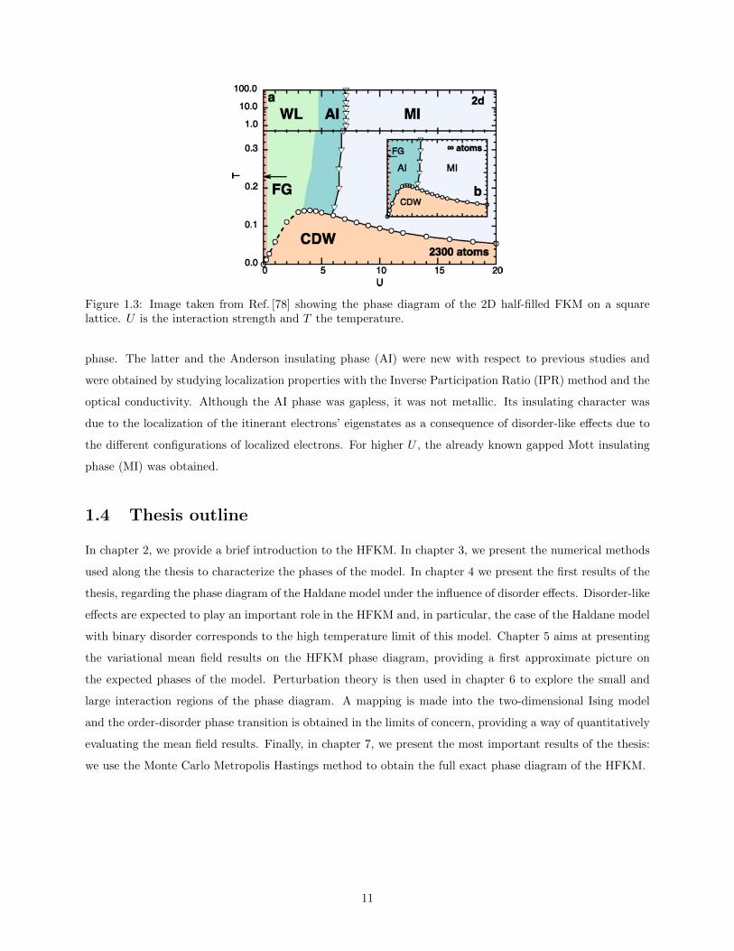
Figure 1.3: Image taken from Ref. [78] showing the phase diagram of the 2D half-filled FKM on a squarelattice. U is the interaction strength and T the temperature.

phase. The latter and the Anderson insulating phase (AI) were new with respect to previous studies and

were obtained by studying localization properties with the Inverse Participation Ratio (IPR) method and the

optical conductivity. Although the AI phase was gapless, it was not metallic. Its insulating character was

due to the localization of the itinerant electrons’ eigenstates as a consequence of disorder-like effects due to

the different configurations of localized electrons. For higher U , the already known gapped Mott insulating

phase (MI) was obtained.

1.4 Thesis outline

In chapter 2, we provide a brief introduction to the HFKM. In chapter 3, we present the numerical methods

used along the thesis to characterize the phases of the model. In chapter 4 we present the first results of the

thesis, regarding the phase diagram of the Haldane model under the influence of disorder effects. Disorder-like

effects are expected to play an important role in the HFKM and, in particular, the case of the Haldane model

with binary disorder corresponds to the high temperature limit of this model. Chapter 5 aims at presenting

the variational mean field results on the HFKM phase diagram, providing a first approximate picture on

the expected phases of the model. Perturbation theory is then used in chapter 6 to explore the small and

large interaction regions of the phase diagram. A mapping is made into the two-dimensional Ising model

and the order-disorder phase transition is obtained in the limits of concern, providing a way of quantitatively

evaluating the mean field results. Finally, in chapter 7, we present the most important results of the thesis:

we use the Monte Carlo Metropolis Hastings method to obtain the full exact phase diagram of the HFKM.

11

Chapter 2

Haldane-Falicov-Kimball model

2.1 Hamiltonian

f-electronc-electronHaldane

fluxes

U

U − t

t2eiϕ

− t

− t

ϕ

Figure 2.1: Sketch of the HFKM. The large red particles correspond to f-electrons (localized) and the greenparticles to c-electrons (itinerant). The Haldane fluxes φij = ±φ are represented by the blue arrows. Thesefluxes are as defined in section 1.3.2 and the arrows indicate their sign: if a c-electron hops in the directionof the arrow, the sign is positive, otherwise, it is negative. There is an energy cost of U for a c-electron tohop into a site occupied with a f-electron due to the on-site interactions between these fermionic species, alsorepresented in the figure.

The Hamiltonian for the HFKM is:

H = −t∑〈i,j〉

c†i cj + t2∑〈〈i,j〉〉

eiφijc†i cj + h.c.+ η∑i

ζic†i ci

+ U∑i

c†i cinf,i −∑i

(µcc†i ci + µfnf,i) .

(2.1)

As suggested in the previous chapter, this Hamiltonian depicts a species of itinerant electrons (c-electrons)

with creation operators c†i and another of localized electrons (f-electrons) whose local density at site i is given

by the number nf,i. The operators ci = ci,A, ci,B are defined in the two interpenetrating triangular sublattices

A and B that form the honeycomb lattice (Fig. 1.2). In contrast to the localized f-electrons, c-electrons can

hop between first and second neighbor sites, as sketched in Fig. 2.1. These hoppings are accounted for in the

12

first and second terms in the Hamiltonian. As already described in the introductory chapter for the Haldane

model, the phases/fluxes φij = ±φ ∈] − π, π] are built in such a way that the total flux in the unit cell is

zero. Their sign is determined by the arrows represented in Fig. 2.1 (see caption). The third term in the

Hamiltonian considers a staggered potential ηζi, where ζi = ±1 respectively for sites of type A and B. The

fourth term describes the local interaction between the localized and itinerant electrons, and the final term

contains the chemical potentials for the itinerant and localized electrons, respectively µc and µf as described

in section 1.7. In what follows, we respectively use c-eletrons (f-electrons) and itinerant (localized) electrons

interchangeably.

2.2 Particle-hole symmetry

We want to study the Hamiltonian at half-filling. A way of getting the values of the chemical potentials that

guarantee half-filling is by inspecting for which conditions the Hamiltonian has particle-hole (PH) symmetry.

The particle-hole transformation can be written as

ciA →− ch†iB

ciB →ch†iA

fi →(−1)p(i)fh†i ,

(2.2)

where p(i) = 0 for i ∈ A and p(i) = 1 for i ∈ B.

Taking into account that first neighbors are always in different sublattices, the first neighbor hopping

term is PH symmetric as

t∑〈i,j〉

c†i cj → t∑〈i,j〉

ch†i chj .

If we now apply the PH transformation to the second neighbor hoppings’ term and use the fact that it

only couples lattices of the same type, we arrive at:

t2∑〈〈i,j〉〉

(eiφijc†i cj + e−iφijc†jci)→ t2∑〈〈i,j〉〉

(−eiφijch†j chi − e−iφijc

h†i c

hj ) .

In this case, the symmetry only occurs for eiφij = −e−iφij , that is φij = ±π/2. For the term with the

staggered potential η, we have

η∑i∈A

c†iAciA − η∑i∈B

c†iBciB → η∑i∈B

(−ch†iBchiB)− η

∑i∈A

(−ch†iAchiA) ,

therefore being PH symmetric. Finally, the interaction term becomes:

U∑i

c†i cinf,i → U∑i

ch†i chi f

h†i fhi − U

∑i

(ch†i chi + fh†i fhi ) .

13

If we further take into account that the terms with the chemical potentials transform as µc → −µc and

µf → −µf , the total Hamiltonian part containing density operators for itinerant and localized electrons is

PH symmetric if:

µc,f = −µc,f + U → µc,f =U

2.

In summary, the whole Hamiltonian is PH symmetric if

φij = ±π/2 (2.3)

µc = µf =U

2

2.3 Half-filling

The FKM is an approximation of the Hubbard model in which one of the spin species of electrons corresponds

to localized (“massive”) particles. In the case of the Hubbard model, half-filling occurs when we have electrons

occupying every site (because each site can have two electrons with opposite spin). It is then natural that

for the half-filled case of the FKM, the average numbers of localized and itinerant electrons are N/2, with

N being the total number of lattice sites. From particle-hole symmetry we can already extract some simple

conditions in order to satisfy half-filling. If the Hamiltonian is PH symmetric, then we know that it is

unchanged when we make the transformation c†i ci → 1 − c†i ci and nf,i → 1 − nf,i in connection with the

conditions in expression 2.3. It is then easy to see that we have (with the parameters in units of t):

ρc(µc) = 1− ρc(−µc + U) , (2.4)

ρf (µf ) = 1− ρf (−µf + U) . (2.5)

In the expressions above, ρc = 〈 1N

∑i c†i ci〉 and ρf = 〈 1

N

∑i nf,i〉. Therefore, the second condition in

expression 2.3 for the chemical potentials reproduce a half-filling condition (ρc = ρf = 1/2), regarding the

first condition (φ = π/2) is fulfilled.

2.4 Partition function

To write the partition function of the HFKM, we can start by noticing that nf,i commutes with the Hamil-

tonian, that is, [nf,i, H] = 0. This means that the densities nf,i are conserved quantities and can be seen as

a classical variables, assuming values nf,i = 0, 1. The grand-canonical partition function can then be written

as

14

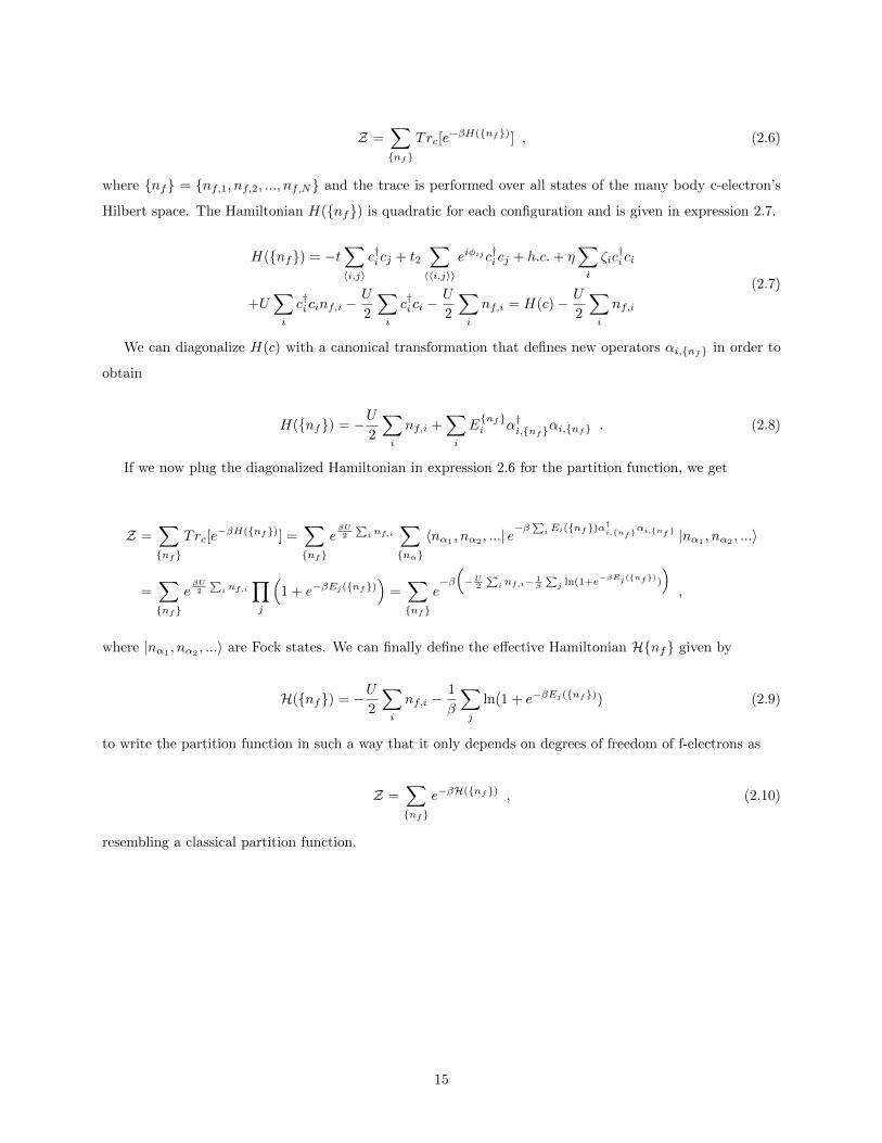
Z =∑nf

Trc[e−βH(nf)] , (2.6)

where nf = nf,1, nf,2, ..., nf,N and the trace is performed over all states of the many body c-electron’s

Hilbert space. The Hamiltonian H(nf) is quadratic for each configuration and is given in expression 2.7.

H(nf) = −t∑〈i,j〉

c†i cj + t2∑〈〈i,j〉〉


ζic†i ci

+U∑i

c†i cinf,i −U

2

∑i

c†i ci −U

2

∑i

nf,i = H(c)− U

2

∑i

nf,i

(2.7)

We can diagonalize H(c) with a canonical transformation that defines new operators αi,nf in order to

obtain

H(nf) = −U2

∑i

nf,i +∑i

Enfi α†i,nfαi,nf . (2.8)

If we now plug the diagonalized Hamiltonian in expression 2.6 for the partition function, we get

Z =∑nf

Trc[e−βH(nf)] =

∑nf

eβU2

∑i nf,i

∑nα

〈nα1 , nα2 , ...| e−β

∑i Ei(nf)α

†i,nf

αi,nf |nα1 , nα2 , ...〉

=∑nf

eβU2

∑i nf,i

∏j

(1 + e−βEj(nf)

)=∑nf

e−β(−U2

∑i nf,i−

1β

∑j ln(1+e−βEj(nf))

),

where |nα1 , nα2 , ...〉 are Fock states. We can finally define the effective Hamiltonian Hnf given by

H(nf) = −U2

∑i

nf,i −1

β

∑j

ln(1 + e−βEj(nf)) (2.9)

to write the partition function in such a way that it only depends on degrees of freedom of f-electrons as

Z =∑nf

e−βH(nf) , (2.10)

resembling a classical partition function.

15

Chapter 3

Methods

Obtaining the phase diagram of the HFKM requires an extensive numerical analysis to grasp into all the

relevant phases of the model. In order to complete this task, one has to search for charge ordering and study

topological, spectral and localization properties, a process that requires a significant amount of methods.

We can divide our study in two main components: observables related to localized f-electrons and itinerant

c-electrons. Regarding f-electrons, we are mainly interested in finding the domain of existence of the charge

ordered CDW phase. To do that, both the approximate variational mean field and exact Monte Carlo

methods are used.

The study of the c-electrons’ properties is also carried out in the frameworks of both the mean field

(MF) and Monte Carlo (MC) methods. The main idea is to use the special feature of the FK interactions to

generate numerically f-electron configurations according to the Boltzmann weights of the mean field and exact

effective f-electron Hamiltonians respectively with the MF and MC methods. The observables of c-electron

can then be obtained by averaging on a large enough set of generated configurations that correspond to the

most likely f-electron states for a given interaction strength U and temperature T . In this way, methods that

are often used for disordered systems can be employed in our model to compute c-electron observables with

the difference that the averaging process is applied on configurations generated according to the Boltzmann

weights and not on disorder realizations. With this purpose, widely used methods to study densities of states,

localization and topology in disordered systems are presented in section 3.3.

This chapter is dedicated to describe the numerical methods used to obtain the phase diagram of the

HFKM. The aim is to provide a general overview of these methods and of their implementation to the reader

that is unfamiliar with them.

3.1 Variational mean field method

The variational mean field method proposes a mean field Hamiltonian HMF written in terms of a set of

variational parameters computed to better describe the original system [79].

16

The Bogoliubov inequality for the free energy, given in expression 3.1 settles the basis for the application

of the variational mean field method [80]. In this expression, FMF = − 1β ln(ZMF ) and 〈〉MF is the average

on the thermal distribution ρMF = e−βHMF .

F ≤ FMF + 〈H −HMF 〉MF ≡ F (3.1)

Based on the Bogoliubov inequality, we need to find the values of the set of parameters chosen for

HMF that minimize the functional F also defined in expression3.1. In that way, we define the mean field

Hamiltonian HMF that better approximates the exact Hamiltonian.

For the HFKM, we propose the mean field Hamiltonian given in expression 3.2 to approximate the effective

Hamiltonian H defined in expression 2.9, where the single variational parameter ω is introduced.

HMF = −ω∑i∈A

nf,i + ω∑i∈B

nf,i (3.2)

This Hamiltonian favors sublattice A if ω > 0. One must notice that HMF provides a mean field

approximation for the effective Hamiltonian H for which the c-electrons’ degrees of freedom are already

integrated out. This means that the interactions between localized and itinerant electrons from the initial

HFKM Hamiltonian are hidden in the form of an effective field ω that acts on each f-electron. In the

disordered phase, both sublattices will be on average equally occupied and we must have ω = 0. On the

other hand, in the ordered CDW phase one sublattice will be more occupied and therefore ω 6= 0. The value

of ω can be determined by minimizing the functional F defined in expression 3.1 for a given set of parameters.

The partition function for the mean field Hamiltonian is

ZMF =∑nf,i

e−βHMF =

( ∑nAf,i

eβω∑i∈A nf,i

)( ∑nBf,i

e−βω∑i∈B nf,i

)

= [(1 + eβω)(1 + e−βω)]N/2 = (2 + 2 cosh(βω))N/2 .

(3.3)

We can also calculate FMF and 〈HMF 〉MF through:

FMF = − 1

βln(ZMF ) = −N

2βln(2 + 2 cosh(βω)) (3.4)

〈HMF 〉MF =

∑nf,iHMF e

−βHMF∑nf,i e

−βHMF= − ∂

∂βln(ZMF ) = −N

2

ω sinh(βω)

1 + cosh(βω)(3.5)

The only quantity left to compute in order to obtain F is 〈H〉MF . This is done numerically. The procedure

is to diagonalize H for a finite system and for a fixed configuration nf to write H in the form defined in

expression 2.9. To compute 〈H〉MF , we will be interested in generating uncorrelated configurations of f-

electrons in order to obtain the average on the thermal distribution ρMF = e−βHMF . These configurations

are generated in each sublattice with the requirement that the average occupation of sublattices A and B is

17

given by

〈nAf,i〉MF =eβω

1 + eβω= nFD(−βω) (3.6)

〈nBf,i〉MF =e−βω

1 + e−βω= nFD(βω) , (3.7)

where nFD is the Fermi-Dirac distribution. Notice that 〈nAf,i〉MF + 〈nBf,i〉MF = 1 as required by the half-

filling requisite. 〈H〉MF can then be computed by taking the thermal average of H for a large enough set of

configurations satisfying expressions 3.6 and 3.7:

〈H〉MF =

∑nf,iH(nf)e−βHMF∑

nf,i e−βHMF

. (3.8)

We can further define the order parameter δ = 〈nAf,i〉MF − 〈nBf,i〉MF corresponding to the difference

between the f-electron occupations in sublattices A and B. In terms of the variational parameter ω, it is

given by:

δ = 〈nAf,i〉MF − 〈nBf,i〉MF =sinh(βω)

1 + cosh(βω).

The average occupation for sublattices A and B can be written in terms of the order parameter δ in a

simplified way,

〈nAf,i〉MF =1 + δ

2

〈nBf,i〉MF =1− δ

2

(3.9)

meaning that they only depend on the value of δ, that is, on the value of βω.

3.2 Monte Carlo Metropolis Hastings

In this section we describe the classical Monte Carlo Metropolis Hastings (MC) algorithm used in chapter

7. First of all, it is important to stress out why we can use a classical MC algorithm for the HFKM. The

reason has already been suggested multiple times in the text and it lies on the fact that we can integrate

out the c-electrons’ degrees of freedom to write the partition function of the system as a sum of the classical

configurations of f-electrons after defining the effective Hamiltonian H(nf) as shown in expression 2.10.

The aim of the MC method is to generate states/configurations according to the Boltzmann distribution.

The way these states are sampled is by setting up a Markov chain for which configurations are generated

according to the Boltzmann weights

Peq(nf) =e−βH(nf)

Z, (3.10)

18

where nf is a given configuration for the system’s classical degrees of freedom and H and Z are respectively

the system’s effective Hamiltonian and partition function. A key feature of a Markov chain is that the

probability of a given new configuration only depends on the preceding one. It must obey the detailed

balance condition given by

Peq(nf)W (nf → nf′) = Peq(nf′)W (nf′ → nf) , (3.11)

where W (nf → nf′) is the transition probability from configuration nf to nf′.

Provided that condition 3.11 is satisfied, the expectation value of a given quantity can be estimated as a

mean over the Markov chain of N elements. Given some observable A, we then have

〈A〉 =∑nf

Peq(nf)A(nf) ≈1

N

N∑k=1

A(nfk) . (3.12)

There are many ways to generate a Markov chain, but we are interested in using a local update algorithm

for which updates are proposed for a single degree of freedom. For the Metropolis-Hastings algorithm, the

transition probability between configurations is

W (nf1 → nf2) =

1 E2 < E1

e−β(E2−E1) E2 ≥ E1

(3.13)

and one can easily verify that it satisfies condition 3.11.

The implementation of this method is then very straightforward:

1. A random configuration is generated as a first step and the corresponding energy E1 is computed;

2. The occupancy of a single site is updated and the energy of the new configuration E2 is computed;

3. E2 is compared with E1 and the new configuration is accepted with the probability given in expression

3.13;

4. The steps 2-3 are repeated.

An initial period of thermalization occurs until the system reaches equilibrium and the states start being

sampled according to the partition function. After equilibration, measurements of thermodynamic quantities

can be carried out. Finally, it must be taken into account that there is a correlation time τ associated

with consecutive generated configurations corresponding to an estimate of the time interval for which these

are correlated. In fact, for N consecutive measurements, only N/2τ correspond to effective uncorrelated

configurations and this must be taken into account when computing the measurement errors (see Appendix

C.3 for details).

19

3.2.1 Binder cumulants

The computation of the critical temperature with the Monte Carlo method is carried out through an analysis

of Binder cumulants. These quantities are computed in terms of an order parameter ∆ which in our case can

be defined as the difference between the occupations in sublattices A and B of the honeycomb lattice (see

Fig. 1.2a). The Binder cumultant U4 can then be defined in terms of this order parameter as

U4 = 1− 〈∆4〉3〈∆2〉2

. (3.14)

This quantity provides a very useful way of determining critical temperatures Tc numerically because it

scales according to [81]

U4 = fU4(x)[1 + · · · ] ,

where x = (β − βc)L1/ν is the scaling variable, with βc = 1/(kBTc) ,L the system’s linear size and ν the

critical exponent associated with the correlation length ξ (ξ ∝ Aξ|T − Tc|−ν). The · · · represent finite-size

corrections that become negligible for a large enough system size. This scaling behaviour means that for

T = Tc, the binder cumulants have the same value for different system sizes. The critical temperature can

then be determined as being the intersection point between Binder cumulants computed for different system

sizes.

20

3.3 Methods for computing c-electron’s observables

As we have already discussed, the different configurations of f-electrons act as a disorder-like potential to

the c-electrons. In sections 3.1 and 3.2 we introduced ways of respectively generating mean field and Monte

Carlo configurations for the f-electrons. These configurations are generated for a given interaction strength

U and temperature T and provide a way of numerically computing all the relevant c-electron’s observables

for this set of parameters.

3.3.1 Coupling matrix method to compute the Chern number

To obtain the topological phases existing in the HFKM it is essential to have a way of computing the

topological invariant introduced in section 1.1.4 - the Chern number. The idea is to compute the Chern

number for the c-electrons by averaging on the f-electron configurations generated with the MF and MC

methods. This means that special care must be taken when computing this quantity as the system is not,

in general, translational invariant for a given configuration. To address this issue, the method introduced

in Ref. [82] to compute the Chern number for disordered systems is used. In this section, this method is

described and the advantages with respect to other possible methods are briefly discussed.

We start by considering a system with a Hamiltonian H and eigenstates |un〉 such that H |un〉 = En |un〉.

We assume that the system depends on a set of parametersR that can be tuned adiabatically. IfR = (Rx, Ry)

is a vector defined in a 2D space and if the system is periodic in R, the usual expression to compute the

Chern number for a given state |Ψn〉 is

Cn =1

2π

∫SdS ·Ω(n)(R) , (3.15)

where S corresponds to the system’s unit cell and Ω is the Berry curvature defined in section 1.1.4. When

translational invariance is broken, we must work in real space and a standard useful approach is to use twisted

boundary conditions,

uθn(r + Liai) ≡ 〈r + Liai|uθn〉 = eiθiuθn(r) ,

where we introduced the parameters θ = (θx, θy) and ai are basis vectors of the direct lattice.

We are interested in computing the Chern number in the ground state |Ψθ〉 of the many body system. It

can be written explicitly as

|Ψθ〉 =

M∏i=1

ϕ†n(θ) |0〉 . (3.16)

where M corresponds to the total number of occupied states and |0〉 is the vacuum state. The operators

ϕ†n(θ) are defined in such a way that |uθn〉 = ϕ†n(θ) |0〉, with |uθn〉 being the eigenstates of the system for a

set of parameters θ. Expression 3.15 can then be written in terms of the Berry connection A, with R = θ,

21

as

C =1

2π

∫∂Sdlθ ·A(θ) , (3.17)

where A(θ) = 〈Ψθ| i∇θ |Ψθ〉. In this form, an efficient discretized version of A(θ) can be found.

We start by considering a path λ = λ(θ) enclosig the surface Sθ and calculate the Chern number in a

system enclosed by this path using expression 3.17. First, we discretize the continuum of states in the path,

as shown in Fig. 3.1a.

(a) (b)

Figure 3.1: a, Discretization of the Sθ surface boundary. The gray spots represent the discretized states,separated by ∆lx or ∆ly. b, Discretization of the surface Sθ in small plaquettes that correspond to loopsin the discretized states. Notice that the sum of the fluxes in every plaquette yields only the flux at theboundary (path λ(θ)) as the interior contributions cancel. This can be seen in the example of the red andgreen plaquette. In this illustrative example, we have a system with Nx = Ny = 5 plaquettes.

A way to find a discretized form for expression 3.17 is by noticing that, to first order in the vector ∆l

separating discretized states:

∆l · 〈Ψθ|∇θΨθ〉 ≈ ln[1 + ∆l · 〈Ψθ|∇θΨθ〉

]= ln

[〈Ψθ| (|Ψθ〉+ ∆l · |∇θΨθ〉)

]= ln

[〈Ψθ|Ψθ+∆l〉

].

In this way we can use a small enough ∆l to compute the Chern number numerically in the path λ(θ).

One must however notice that 〈Ψθ|∇θΨθ〉 is a pure imaginary quantity because

Re[〈Ψθ|∇θΨθ〉

]=

1

2

[〈Ψθ|∇θΨθ〉+ 〈∇θΨθ|Ψθ〉

]=

1

2∇θ 〈Ψθ|Ψθ〉 = 0 .

We must then make sure that only the imaginary part of the discretized result is considered. If we

write the so called link variable 〈Ψθ|Ψθ+∆l〉 as a general complex number z = |z|ei arg(z), the discretization

becomes:

22

∆l · 〈Ψθ|∇θΨθ〉 → iIm[ln 〈Ψθ|Ψθ+∆l〉] = i arg 〈Ψθ|Ψθ+∆l〉 .

With this approach, we can transform the integration in expression 3.17 into a product in the link variables

of the discretized states along the path:

C =1

2π

∫∂Sdlθ · 〈Ψθ| i∇θ |Ψθ〉 → −

1

2π

∑n

arg 〈Ψθn |Ψθn+∆ln〉 = − 1

2πarg

(∏n

〈Ψθn |Ψθn+∆ln〉

),

where θn+1 = θn+∆ln and we used arg(a)+arg(b) = arg(ab). To compute the link variables 〈Ψθn |Ψθn+∆ln〉,

we can recall expression 3.16 and notice that the eigenstates |uθn〉 can also be written in terms of the local

site basis ri as

|uθn〉 =∑ri

ϕn,θri |ri〉 .

The link variables are then given by the following Slater determinant:

〈Ψθn |Ψθn+∆ln〉 = det(

Φ†θnΦθn+∆ln

), (3.18)

where matrix Φθ is defined in terms of the amplitudes ϕn,θri as:

Φθ =

ϕ1,θr1 ϕ2,θ

r1 ... ϕM,θr1

ϕ1,θr2 ϕ2,θ

r2 ... ϕM,θr2

. . .

. . .

. . .

ϕ1,θrN ϕ2,θ

rN ... ϕM,θrN

.

A possible approach to implement our discretization procedure is to discretize the surface Sθ in NxNy

small plaquettes as represented in Fig. 3.1b, compute the Chern number in each plaquette and sum them all.

If we label each plaquette with index µ, the Chern number in plaquette µ will be:

Cµ =− 1

2πarg(〈Ψθµ |Ψθµ+∆lx〉〈Ψθµ+∆lx |Ψθµ+∆lx+∆ly 〉〈Ψθµ+∆lx+∆ly |Ψθµ+∆ly 〉〈Ψθµ+∆ly |Ψθµ〉

).

(3.19)

The total Chern number will simply be given by C =∑µ Cµ. This is a good approach if we have

translational invariance as we can immediatly identify the eigenstates with the k vector. But as it has

already been stated, in our case we cannot do that and must work in the real space basis |ri〉, therefore with

23

matrices Φθ. This brings some difficulties to the problem. Using expression 3.18, expression 3.19 can be

written in terms of the Φθ matrices as

Cµ =− 1

2πarg det

(Φ†θµΦθµ+lxΦ†θµ+lx

Φθµ+lx+lyΦ†θµ+lx+lyΦθµ+lyΦ†θµ+ly

Φθµ

)= − 1

2πarg det(Φµpl) .

(3.20)

The most simple way to compute Cµ is by obtaining the set λµp of eigenvalues of Φµpl and use det Φµpl =∏Mp=1 λp to write:

Cµ = −M∑p=1

arg(λp) .

We would have to diagonalize M×M matrices NxNy times. In the method proposed in Ref. [82], however,

a single diagonalization is required. Using the momentum basis

|uθn〉 =∑ki

Fn,θki |ki〉 , (3.21)

the allowed momenta for twisted boundary conditions are

k =m

Lxbx +

n

Lyby + q ,

where bx = (2π, 0) and by = (0, 2π) are reciprocal lattice vectors, n and m are integers and

q =θx

2πLxbx +

θy2πLy

by .

Writing k = k(0) + q, where k(0) are the allowed momenta for periodic boundary conditions (θ = 0),

expression 3.21 becomes

|uθn〉 =∑ki

Fn,qk(0)i

|k(0) + q〉 .

In a similar way to the link variables 〈Ψθn |Ψθn+∆ln〉 (expression 3.18), the overlaps 〈Ψqn |Ψqn+∆ln〉 can

be written as

〈Ψqn |Ψqn+∆ln〉 = det(Φ†qnΦqn+∆ln

), (3.22)

where

24

Φq =

F 1,q

k(0)1

F 2,q

k(0)1

... FM,q

k(0)1

F 1,q

k(0)2

F 2,q

k(0)2

... FM,q

k(0)2

. . .

. . .

. . .

F 1,q

k(0)N

F 2,q

k(0)N

... FM,q

k(0)N

.

We now apply the exact same procedure used for discretizing Sθ to the Sq surface, considering again

NxNy plaquettes:

qx =n

Nx

1

Lx, n ∈ 0, ..., Nx

qy =m

Ny

1

Ly, m ∈ 0, ..., Ny

q =qxbx + qyby

In a similar way to expression 3.20, we can write the Chern number in plaquette µ as

Cµ =− 1

2πarg det

(Φ†qµΦqµ+∆lxΦ†qµ+∆lx

Φqµ+∆lx+∆lyΦ†qµ+∆lx+∆lyΦqµ+∆lyΦ†qµ+∆ly

Φqµ

).

In this way, we would again need to sum in the NxNy plaquettes. That would not add any simplification

with respect to expression 3.20. The key point now is that if Lx and Ly are sufficiently large, it is a good

approximation to consider a single plaquette instead of NxNy, as if we do this, the four corner points given

in expression 3.23 already define a small enough plaquette.

q0 = (0, 0)

q1 = (2π/Lx, 0)

q2 = (2π/Lx, 2π/Ly)

q3 = (0, 2π/Ly)

(3.23)

Also, once these q vectors belong to the set of allowed momenta for periodic boundary conditions (k(0))

we can calculate the link variables using results for periodic boundary conditions in real space. Noticing that

〈Ψ†q|Ψq′〉 = det(Φ†qΦq′) and writing Φ†qΦq′ = Cq,q′ (coupling matrix), we have

Cm,nq,q′ =∑k(0)i

[Fm,qk(0)i

]∗Fn,q

′

k(0)i

.

Finally, we can write

25

ϕn,θ=0ri =

∑k(0)i

Fn,q=0

k(0)i

eik(0)i ·ri ,

where ϕn,θ=0ri corresponds to the set of the eigenvector amplitudes in the real space local basis |ri〉 for

periodic boundary conditions (θ = 0). It is then easy to show that

Cm,nq,q′ =∑ri

[ϕm,θ=0ri

]∗ei(q−q′)·riϕn,θ=0

ri . (3.24)

The problem reduces to compute the matrix elements of the coupling matrices Cq,q′ , which can be done

with the usage of expression 3.24 by diagonalizing the Hamiltonian matrix defined in basis |ri〉 with periodic

boundary conditions. Defining the matrix

F = Cq0q1Cq1q2Cq2q3Cq3q0

and computing its set of eigenvalues λp, the Chern number becomes

C = − 1

2π

M∑p=1

arg λp .

3.3.2 Recursive method for computing the DOS

In this section we describe an efficient method to compute numerically the DOS that is widely used along

the thesis. It is known as the Recursive method [83, 84].

We start by introducing the concept of local density of states ρr(E) (LDOS) in expression 3.25 where Ei

and |ui〉 are respectively the eigenvalues and eigenstates of the Hamiltonian matrix expressed in the local

site basis |r〉:

ρr(E) =∑i

| 〈ui|r〉 |2δ(E − Ei) . (3.25)

The Green’s function is defined in the usual way as

G(E) = (E −H)−1 . (3.26)

We define Gr(E) as the diagonal matrix element of the Green’s function in the local state |r〉, that is,

Gr(E) = 〈r|G(E) |r〉 . (3.27)

This quantity is useful as we can relate it to the LDOS through

ρr(E) = − 1

πlimη→0

ImGr(E + iη) , (3.28)

26

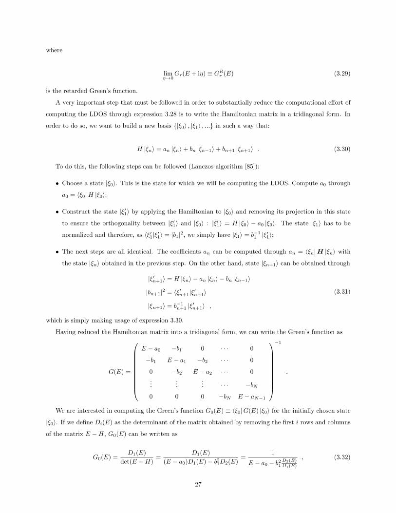
where

limη→0

Gr(E + iη) ≡ GRr (E) (3.29)

is the retarded Green’s function.

A very important step that must be followed in order to substantially reduce the computational effort of

computing the LDOS through expression 3.28 is to write the Hamiltonian matrix in a tridiagonal form. In

order to do so, we want to build a new basis |ξ0〉 , |ξ1〉 , ... in such a way that:

H |ξn〉 = an |ξn〉+ bn |ξn−1〉+ bn+1 |ξn+1〉 . (3.30)

To do this, the following steps can be followed (Lanczos algorithm [85]):

• Choose a state |ξ0〉. This is the state for which we will be computing the LDOS. Compute a0 through

a0 = 〈ξ0|H |ξ0〉;

• Construct the state |ξ′1〉 by applying the Hamiltonian to |ξ0〉 and removing its projection in this state

to ensure the orthogonality between |ξ′1〉 and |ξ0〉 : |ξ′1〉 = H |ξ0〉 − a0 |ξ0〉. The state |ξ1〉 has to be

normalized and therefore, as 〈ξ′1|ξ′1〉 = |b1|2, we simply have |ξ1〉 = b−11 |ξ′1〉;

• The next steps are all identical. The coefficients an can be computed through an = 〈ξn|H |ξn〉 with

the state |ξn〉 obtained in the previous step. On the other hand, state |ξn+1〉 can be obtained through

|ξ′n+1〉 = H |ξn〉 − an |ξn〉 − bn |ξn−1〉

|bn+1|2 = 〈ξ′n+1|ξ′n+1〉

|ξn+1〉 = b−1n+1 |ξ′n+1〉 ,

(3.31)

which is simply making usage of expression 3.30.

Having reduced the Hamiltonian matrix into a tridiagonal form, we can write the Green’s function as

G(E) =

E − a0 −b1 0 · · · 0

−b1 E − a1 −b2 · · · 0

0 −b2 E − a2 · · · 0...

...... · · · −bN

0 0 0 −bN E − aN−1

−1

.

We are interested in computing the Green’s function G0(E) ≡ 〈ξ0|G(E) |ξ0〉 for the initially chosen state

|ξ0〉. If we define Di(E) as the determinant of the matrix obtained by removing the first i rows and columns

of the matrix E −H, G0(E) can be written as

G0(E) =D1(E)

det(E −H)=

D1(E)

(E − a0)D1(E)− b21D2(E)=

1

E − a0 − b21D2(E)D1(E)

, (3.32)

27

whereD0(E) = det(E−H) is the determinant of the whole matrix, and therefore the structure ofD2(E)/D1(E)

will be the same as the structure of D1(E)/D0(E). The result can then be written as a continued fraction

expansion:

G0(E) =1

E − a0 − b21 1E−a1−b22

1

...···b2N−1

1E−aN−1

. (3.33)

The advantage of this continuous fraction is that the coefficients an and bn converge quickly to fixed

values, that we respectively call a∞ and b∞. This provides a way of terminating the continued fraction. The

terminator t(E) can be computed through

t(E) =b2∞

E − a∞ − t(E). (3.34)

Taking into account that t(E) must go to zero in the E →∞ limit, the only possible solution for equation

3.34 is

t(E) =1

2

((E − a∞)− [(E − a∞)2 − 4|b∞|2]1/2

). (3.35)

We are interested in Hamiltonians associated with two energy bands. In these cases the coefficients an

and bn converge instead to two different values each, that we respectively call a∞,1, a∞,2, b∞,1 and b∞,2. In

these cases, the expression for the terminator corresponds to

t(E) =(E − a∞,1)(E − a∞,2) + b2∞,1 − b2∞,2

2(E − a∞,1)

−

√√√√( (E − a∞,1)(E − a∞,2) + b2∞,1 − b2∞,22(E − a∞,1)

)2

− b2∞,1E − a∞,1E − a∞,2

.

(3.36)

We must now address the choice of the state |ξ0〉 for which we are computing the LDOS. A possible choice

would be to compute the LDOS for all the local states ri and obtain the full DOS through

DOS(E) =1

N

N∑i=1

ρri(E) . (3.37)

In systems with translational invariance, the LDOS ρri(E) is the same for every state ri and the compu-

tation of this quantity for an arbitrary local state corresponds to DOS(E). However, for disordered systems

this is not the case and we would have to compute the LDOS for every local state to obtain the full DOS.

This would substantially increase the computational cost of the method. A clever way to go around this

problem is to generate a random state |ϕ〉 that spans all the Hilbert space of the problem corresponding to

a linear combination of all the local states |ri〉 with random amplitudes φi:

28

n = 1

n = 2

⋮

⋯

⋯

site A

site B

zig-zag wire

NNN hoppings

i

i − 1

i + 1Lo

ngitu

dina

l dire

ctio

n(

uni

t cel

ls)

NL

Transverse direction ( unit cells)M

Figure 3.2: Representation of the zig-zag structures used to define the transfer matrices for the honeycomblattice. The full black line represents a given wire and each wire is labeled by index n. The sites of a givenwire are labeled by index i. The dashed green lines represent some examples of the NNN hoppings of theHaldane model. Notice that these hoppings connect sites in the same wire but also in neighboring chains.

|ϕ〉 =

N∑i=1

φi |ri〉 . (3.38)

Provided that φi are random variables, we have that the average of the LDOS in the random states |ϕ〉

is equal to the DOS, that is, 〈ρϕ(E)〉 = DOS(E). The DOS can then be obtained by averaging ρϕ in two

different ways: one on different sampled configurations and other on a set of random starting states |ϕ〉. In

practice, if the system is large enough, a very small amount of averages is needed due to the self-averaging

property of the DOS.

The recursive method provides a fast way of obtaining the DOS. The fact that it does not involve explicit

diagonalization makes it possible to obtain results for very large systems (of the order of 103 × 103 unit cells

in the case of a 2D system) in a reasonable amount of time.

3.3.3 Transfer Matrix Method (TMM)

In this section we expose the Transfer Matrix Method (TMM). This method is used to study the localization

of the eigenstates of c-electrons and provides a way of classifying them as localized or extended [86]. In

the context of this thesis, it is applied for studies on the Haldane model under the influence of disorder, in

chapter 4 and on the HFKM with the mean field method in chapter 5. We will therefore specify the method

for the disordered Haldane model in the honeycomb lattice for which some simplifications can be introduced

with respect to other tight-binding models involving next nearest neighbor (NNN) hoppings.

We start by considering a quasi-1D system with NL and M unit cells respectively in the longitudinal and

transverse directions, with NL M . A useful way of implementing this system for a honeycomb lattice is

to view it as being composed by zig-zag chains, as represented in Fig. 3.2. The fact that NNN hoppings only

connect neighboring chains in this picture introduces a significant computational advantage with respect to

arrangements that require hoppings between NNN chains, for which larger transfer matrices are necessary.

Using the notation introduced in Fig. 3.2, we can write the Hamiltonian matrix for the quasi-1D system

29

in the form

H =∑n

∑i,j

(|n, i〉 εijn 〈n, j|+ |n+ 1, i〉V ijn+1,n 〈n, j|+ |n, i〉V

ijn,n+1 〈n+ 1, j|

). (3.39)

The |n, i〉 state belongs to the local site basis and corresponds to an orbital at site i of the n-th wire.

The parameters εijn are the matrix elements for a given wire concerning on-site potentials and NN and

NNN hoppings. Vn+1,n and Vn,n+1 are matrix elements between different chains that involve NN and NNN

hoppings. If we write the wavefunction in terms of its amplitudes at each site in the form |Ψ〉 =∑n,iA

in |n, i〉,

the Schrodinger equation becomes:

〈n, i|H |Ψ〉 = E 〈n, i|Ψ〉 ↔∑j

V ijn,n+1Ajn+1 =

∑j

[(Eδij − εijn )Ajn − V

ijn,n−1A

jn−1

]↔ Vn,n+1An+1 = (EI − εn)An − Vn,n−1An−1 ,

(3.40)

where in the last equality the equation was written in a matricial form. We can write this equation in a

different way:

Vn,n+1 0

0 Vn,n+1

An+1

An

=

EI − εn −Vn,n−1

Vn,n+1 0

An

An−1

An+1

An

=

V −1n,n+1(EI − εn) −V −1

n,n+1Vn,n−1

I 0

An

An−1

=Tn

An

An−1

= Mn

A1

A0

.

(3.41)

Remembering that each wire contains 2M sites, we can verify that the matrix Tn defined in expression

3.41 is a 4M × 4M matrix - the so called transfer matrix of the quasi-1D dystem - and Mn is the product of

all the transfer matrices from Tn to T1. Mn satisfies Oseledec’s theorem [87] that guarantees the existence

of the limiting matrix Γ such that

Γ = limNL→+∞

(MNLM†NL

)1

2NL . (3.42)

This matrix has eigenvalues exp(γi) with i = 1, ..., 2M and γi being the Lyapunov exponents of matrix

MNL . These exponents describe the exponential increase (if γi > 0) or decrease (if γi < 0) of the wavefunction

amplitudes Ain along the quasi-1D system. We are interested in the exponents describing the exponential

increase of the wavefunctions, and therefore the ones satisfying γi > 0. For a given size M , we identify these

exponents as the inverse of the localization length λM . The smallest exponent, minγi, corresponds to the

largest localization length and hence to the localization length of the system (λ−1M = minγi). The study

of the λM/M behaviour for a given state can determine if it is localized. If ΛM = λM/M decreases with M ,

30

then we are sure that the state will remain localized for M → +∞. If, on the other hand, ΛM increases or

does not change with M , the localization length will grow at an equal or higher rate than the system’s size

and the state will be extended.

Based on the information exposed up to this point, our task should be simply to compute the Lyapunov

exponents through products of transfer matrices onto an arbitrary initial vector. However, this product will

converge towards the largest eigenvalue of MNL which is associated with the fastest exponential increase and

our aim is to seek for the smallest. A possible way to do so is to repeatedly multiply the transfer matrices

onto 2M orthogonal initial vectors |An〉 in order to access all the Lyapunov exponents. The problem with

this method is that the ratio between the smallest and largest eigenvalues of MNL becomes comparable with

the machine precision after few products due to their exponential increase. This means that the smallest

eigenvalue would quickly be lost. To solve this, we can make a QR decomposition of the matrix MNL for

every k products, where Q is an orthonormal matrix (Q†Q = I) and R is an upper triangular matrix. After

performing this decomposition, we arrive at

MNL =

NL∏i=1

Ti =

(NL∏

i=k+1

Ti

)(k∏i=1

Ti

)=

(NL∏

i=k+1

Ti

)Q(1)R(1) =

(NL∏

i=2k+1

Ti

)(2k∏

i=k+1

TiQ(1)

)R(1)

=

(NL∏

i=2k+1

Ti

)Q(2)R(2)R(1) = ... = Q(n)

n∏i=1

R(i) ≡ Q(n)R(n) ,

(3.43)

where n = NL/k is the number of QR decompositions. If we consider |vi〉 to be the eigenvector of matrix Γ

with corresponding eigenvalue exp(γi), we have

limNL→+∞

1

NLln ||MNL |vi〉 || = γi . (3.44)

Assuming that the Lyapunov exponents are ordered in ascending order, that is, γ1 ≤ γ2 ≤ · · · ≤ γ2M , it

can be shown through expression 3.44 that

limn→+∞

1

nkln(Rll

(n)) ≡ lim

n→+∞

1

nk

n∑i=1

ln(R(i)ll ) = γ2M−l−1 , (3.45)

where R(n)ll =

∏ni=1R

(i)ll . In this way, we only need to store the diagonal entries of the upper triangular

matrices R(n) everytime a QR decomposition is made (every k iterations) to compute all the Lyapunov

exponents and then select the smaller positive one. Typically, using k = 10 is sufficient not to lose information

on minγi. The choice of NL on the other hand can be made by studying the convergence of λM . To do

this, we introduce the coefficients ci and di:

31

c(i)1 = lnR

(1)ii

c(i)j =c

(i)j−1 + lnR

(j)ii , j = 2, ..., n

d(i)1 =

(lnR

(1)ii

)2

d(i)j =d

(i)j−1 +

(lnR

(j)ii

)2

, j = 2, ..., n .

(3.46)

The variance of the random variables lnR(1)ii , ..., lnR

(n)ii is given by

∆(i)n =

√√√√d(i)n

n−

(c(i)n

n

)2

. (3.47)

We are interested in studying the convergence of λ−1M = minγi = cn

nk which is just the average of the

random variables already introduced (divided by k). Knowing that the standard deviation of the average

cn/n is ∆n/√n, the relative error of λ−1

M is

ε =∆n√n

cn. (3.48)

For the computations carried out throughout the thesis, the longitudinal dimension N of the system was

considered to be the minimum necessary for ε < 1%.

As a final remark, the TMM is also an important tool to study disorder-driven topological phase tran-

sitions. As mentioned in section 1.3.3, the Haldane model belongs to the unitary class and even though

adding disorder closes the topological gap, it does not immediately destroy the topological phase [88]. What

happens is that all states become localized except for two bulk extended states, one belonging to each energy

band. These carry opposite Chern numbers, which means that the system is in a topological phase if the

Fermi level lies between them. If we further increase the disorder strength, the extended states will merge

leading to the destruction of the topological phase. Identifying the extended states is therefore a useful way

of knowing for which parameters the topological phase transition takes place. The TMM provides a way of

doing so as these states can be identified as having a constant ΛM = λM/M as a function of the transverse

system size M . The extended states will merge at the center of the spectrum and therefore, at half-filling,

the task of identifying the topological phase transition reduces to obtaining the set of parameters for which

a constant ΛM as a function of M is observed. Taking this into account, the TMM is used in what follows to

cross-check the topological results obtained through Chern number computations with the method explained

in section 3.3.1.

3.3.4 Inverse participation ratio (IPR)

The IPR method provides a way of measuring the degree of localization of the eigenstates, similarly to the

TMM. If we write the eigenstate |un〉 of our system in terms of the local site basis |ri〉 as |un〉 =∑i φ

ni |ri〉,

32

the IPR of this state is given by

IPRn =∑i

|φni |4 . (3.49)

If the state is delocalized, one expects φni ∼ V −1/2, with V being the system’s volume, that is, the

wavefunction amplitude is equally distributed along every site. This means that IPRn scales with V −1 for

extended states. On the other hand, if the state is localized, IPRn must scale to a constant that provides an

estimate of the localization length. This is easy to understand in that if the state is localized, only a finite

volume, say VL will be associated with significant amplitudes. Therefore, IPRn must scale to ∼ V −1L . In

particular, in the extreme case for which the state is maximally localized, only one site will have an amplitude

close to 1 and in this case, IPRn would scale to 1.

In practice, this quantity is computed for every eigenstate and a large number of configurations. An IPR

histogram is then obtained by dividing the energy spectrum in narrow energy windows and computing the

average IPR inside each window.

3.3.5 Level spacing statistics (LSS)

LSS is yet another way of measuring the degree of localization of eigenstates based on the Random Matrix

theory [86]. We start by assuming that the system is described by a Hamiltonian matrix H =∑ij Hij |i〉〈j|,

with Hij being random matrix elements. Considering that our Hamiltonian has a set of N eigenvalues Ei

ordered in ascending order in the interval I ∈]E − ∆E , E + ∆E [, with ∆E << ∆EB (full bandwidth) we

can extract information on the correlations between energy levels at energy E by considering the probability

density distribution of the spacings between levels, that is,

P (E,S)dS =1

N − 1

∑i

δ(S −∆Ei)dS , (3.50)

where ∆Ei = Ei+1 −Ei. It is often more convinient to define the normalized level spacing distribution p(s),

with s = S/〈S(E)〉 where 〈S(E)〉 =∫dS SP (E,S) is the average spacing for energy E. If the eigenstates

in the interval I are localized, then the eigenvalues Ei must be completely independent. This observation

alone already provides very important information on the level spacing statistics of localized states: the

probability of finding two eigenvalues with spacing s must follow a Poisson distribution, meaning that in this

case

p(E, s) = e−s . (3.51)

If, on the other hand, the energy interval I has extended states, the eigenvalues Ei are expected to be

correlated and level repulsion will occur. The level spacing distribution can be obtained in this case and only

depends on the symmetries of the Hamiltonian. It is described by the Wigner surmise [86]. The Haldane

33

model belongs to the unitary class, for which time-reversal symmetry is broken and is therefore represented

by a Gaussian unitary ensemble (GUE). In this case, p(s) is given by

p(s) =32

π2s2e−4s2/π . (3.52)

The distribution in expression 3.52 has a variance of σ2/〈s〉2 ≈ 0.178. On the other hand, when the states

become localized we no longer have level repulsion and the variance is larger. In particular, for the Poisson

distribution, σ2/〈s〉2 = 1.

In practice, exact diagonalization, that is, the diagonalization of the Hamiltonian matrix for a finite

system, does not allow for the usage of very large systems and therefore we typically do not have sufficient

statistics in a sufficiently small interval around some energy E to obtain an accurate level spacing distribution

for this energy. To solve this, the method used in Ref. [89] is followed: to obtain a level spacing distribution

for a given energy E, we inspect for every sampled configuration the eigenvalues just above and below

this energy, respectively εEi+1 and εEi . Then we compute the level spacings Sj(E) = (εEi+j+1 − εEi+j), with

j ∈ [−k, k]. A typical choice is k = 2. This is done for every configuration and a level spacing distribution is

obtained after normalizing the spacings to their average value 〈S(E)〉.

The LSS method is particulary useful for systems belonging to the unitary class as for these systems

any degree of uncorrelated disorder is expected to localize every eigenstates except for extended states at

particular energies. In the case of the Haldane model, these states are very important as they carry the

Chern number, as stated before. The LSS method provides a way of identifying them by inspecting which

energies are associated with a level spacing distribution with the GUE variance σ2/〈s〉2 = 0.178.

34

Chapter 4

Disordered Haldane model

This chapter focuses on the study of disorder effects in the Haldane model at half-filling. In particular,

Anderson and binary disorders are considered. Disorder-like effects are expected to play a very important

role in the HFKM and therefore this chapter has the aim of attaining an important insight on how they affect

the Haldane model’s phase diagram. In fact, the study of binary disorder provides a way of obtaining the

high temperature phase diagram of the HFKM for which all the configurations of the f-electrons are equally

probable.

The Hamiltonian for the disordered Haldane model can be written as

H = −t∑〈i,j〉

c†i cj + t2∑〈〈i,j〉〉

eiφi,jc†i cj + h.c.+ η∑i

ζic†i ci +

∑i

ξic†i ci

= H0 +∑i

ξic†i ci ,

(4.1)

where ζi = 1 if i ∈ A and ζi = −1 if i ∈ B. ξ(i) are random site energies distributed according to the

probability distributions:

PW (ξi) = 1W Θ(W/2− |ξi||) , Anderson disorder

PV (ξi) = 12 (δ(V − ξi) + δ(ξi)) , binary disorder

(4.2)

The high temperature HFKM can be seen as the model given in expression 4.1 with binary disorder,

for which the interaction magnitude U plays the role of the disorder strength V defined in the probability

distribution given in expression 4.2.

4.1 Numerical results

In order to study the robustness of the topological phases against disorder effects, the Chern number was

computed numerically with the method exposed in section 3.3.1. The TMM and the Recursive method also

35

exposed in chapter 3 were respectively used for studying the localization of the system’s eigenstates and the

spectrum of c-electrons in order to obtain the full phase diagrams.

4.1.1 Topological phase diagram’s evolution

It is known that topological phases are robust under disorder effects. However, there is also a critical

disorder strength for which they cease to exist and this has been shown specifically for the Haldane model

under multiple studies, specially for Anderson disorder [88, 90–92]. However, it is interesting to know how

the Haldane model’s phase diagram evolves with the disorder strength before the topological phases are

completely destroyed and this has not been explored in any of those studies. Our first numerical studies

were then carried out to obtain the qualitative evolution of the Haldane’s phase diagram as a function of the

disorder strength. The results are shown in Figs. 4.1 and 4.2, respectively for Anderson and binary disorder.

-1.0

-0.5

0

0.5

1.0C

Figure 4.1: Evolution of the Haldane model’s phase diagram with Anderson disorder for a, W/t = 2; b,W/t = 3.5; and c, W/t = 4. The black curves are the phase transition curves of the Haldane model for nulldisorder. The results were obtained in units of t, for t2 = 0.1t. The results in figures a) and b) were obtainedfor a 12× 12 unit cell system while the ones in c) were for a 20× 20 system. 100 disorder configurations wereused in total.

-1.0

-0.5

0

0.5

1.0C

a b c

Figure 4.2: Evolution of the Haldane model’s phase diagram with binary disorder for a, V/t = 2; b, V/t = 2.4;and c, V/t = 2.75. The black curves are the phase transition curves of the Haldane model for null disorder.The results were obtained in units of t, for t2 = 0.1t. The results in figure a) were obtained for a 12× 12 unitcell system while the ones in figures b) and c) were obtained for 20× 20 unit cell systems.

We can see that the topological phases change very little under weak disorder as its effect is still small

for W/t = 2 (Fig. 4.1a), but we can already notice a curious phenomenon: they become enhanced in the η

parameter space, being this effect more visible for φ close to π/2. For higher disorder values, the phases

separate in the φ parameter space (Figs. 4.1b,c) and the enhancement in η for regions near φ = π/2 becomes

larger.

36

Figure 4.3: Example of the Chern number’s curves obtained for different system sizes. For this example,W/t = 1.

For binary disorder, we have the same qualitative phenomena for small to intermediate disorder (Figs. 4.2a,b),

but just before the topological phases are completely suppressed, another interesting phenomenon occurs:

the last regions of the topological phases to survive are for large η (Fig. 4.2c), opposite to Anderson disorder

for which these regions occur for η close to zero (Fig. 4.1c).

4.1.2 Phase diagram in the (W, η) plane

To study the enhancement of the topological phases in the η parameter space in more detail, the phase

diagram in the (W, η) parameter space was obtained for φ = π/2. The phase transition curves were obtained

by varying η for fixed W and vice-versa depending on the regions of the phase diagram. Different system

sizes were used in order to check for convergence and an average over 200 disorder configurations was always

performed. The data points were interpolated with the cubic spline method (see Appendix A.1) and the

phase transition point was considered to be the intersection between the curves corresponding to the larger

systems. An example of the obtained curves is provided in Fig. 4.3. Notice that the transition from C = 1

to C = 0 becomes sharper for larger system sizes and it should be abrupt in the thermodynamic limit.

The phase diagram is shown in Fig. 4.4a. The errors were obtained as detailed in Appendix A.2 and

the points associated with the horizontal and vertical error bars were respectively obtained by varying W

with fixed η and vice-versa. The results imply a peculiar phenomenon: for some values of η > 3√

3t2 (with

η = 3√

3t2 corresponding to the phase transition point for null disorder) we can have a phase transition from

a trivial to a topological insulating phase. This is a typical phenomenon observed in the so called topological

Anderson insulators (TAI) already mentioned in the introductory section 1.3.3 [66]. Although these types

of materials first originated from numerical studies, an analytical approach to describe them was already

proposed [67]. Analysing our results within the framework of this theory provides a way of understanding

them in a more fundamental way under an analytical approach. This study is developed in section 4.2.

37

1 2 3 4 5W/t0.0

0.2

0.4

0.6

0.8

1.0η/t

0.5 1.0 1.5 2.0 2.5 3.0V/t0.0

0.2

0.4

0.6

0.8

1.0

1.2η/t

0.5 1V/t

0.56

0.6

η/t

0.5 1 1.5W/t

0.55

0.58

aη/t

b

Figure 4.4: a, Phase diagram of the Haldane model with Anderson disorder in the (W, η) plane for φ = π/2.b, Phase diagram of the Haldane model with binary disorder in the (V, η) plane for φ = π/2. The insetscorrespond to a zoom in the phase diagrams for small disorder. The thinner brown curves below the numericalresults in the insets correspond to the analytical results obtained with the first order self-consistent Bornapproximation (see section 4.2). The dashed green lines in b) correspond to the regions of the phase diagramfor which the results of the TMM are exemplified in Fig. 4.5. The errors associated with the intersection ofthe two cubic splines used to compute the phase transition points are also shown. Points associated with thehorizontal and vertical error bars were respectively obtained by varying the disorder strength with fixed ηand vice-versa.

4.1.3 Phase diagram in the (V, η) plane

The same study as in the previous section was performed for binary disorder. The results are shown in

Fig. 4.4b. Notice that there is clearly a topological region for large η that is destroyed for larger disorder

strengths than the small η region.

The large V region of the phase diagram was confirmed with the TMM as shown in Fig. 4.5. To apply this

method, a finite system with a fixed large longitudinal dimension is considered and the transverse dimension

M is varied. The longitudinal dimension was chosen as specified in section 3.3.3. The quantity under study

is ΛM = λM/M , where λM is the localization length of the system. If ΛM decreases with M , the system’s

eigenstates are localized in the thermodynamic limit, revealing an insulating behaviour. On the contrary, if

ΛM increases with M , the eigenstates are extended and therefore associated with a metallic behaviour. A

constant ΛM signals a critical point corresponding to the merge of two bulk extended states as described in

section 3.3.3. By looking at Fig. 4.4b, for V/t = 2.5 we are always inside the topological phase for small η and

the phase transition into the topologically trivial phase occurs for η ∼ 0.875, in accordance with Fig. 4.5a for

which we can see that ΛM is constant for that value. On the other hand, for V/t = 2.8, we start at a trivial

phase for small η. By increasing η, we cross the phase transition curve into the topological phase and then

there is another phase transition again to the trivial phase in accordance with Fig. 4.5b. It is also important

to notice that apart from the critical points, ΛM decreases with M showing that the system’s eigenstates are

localized at half-filling and it is in a (topological or trivial) insulating phase.

38

0.2 0.4 0.6 0.8 1.0η/t

- 0.6

- 0.4

- 0.2

ΛMlog

0.4 0.6 0.8 1.0η/t

- 0.3

- 0.2

- 0.1

0.1

M =22

M =26

M =30

M =34

M =38

M =42

M =46

M =50

M =54

M =58

M =62

ΛMloga b

Figure 4.5: Results of the TMM for large values of binary disorder. a, V/t = 2.5; b, V/t = 2.8. The legendindicates the different values of M used. ΛM decreases with M except in the phase transition points forwhich this quantity remains unchanged. This behaviour is the expected for trivial and topological insulatingphases. The single critical point obtained for V/t = 2.5 and the two critical points obtained for V/t = 2.8are in accordance with the results obtained for the Chern number in Fig. 4.4 and are marked with arrows.

0.0 0.5 1.0 1.5 2.0 2.5 3.0 3.5W/t0.0

0.2

0.4

0.6

0.8

1.0

1.2

1.4η/t

Gapped, C=0

Gapped, C=1

Gapless

C=0

C=1A B

0.0 0.5 1.0 1.5 2.0V/t0.0

0.2

0.4

0.6

0.8

1.0

η/t

C

D

EGapped, C=0

Gapped, C=1C=1

C=0Gapless

a b

Figure 4.6: Gapped and gapless regions of the φ = π/2 phase diagrams in the (W, η) (a) and (V, η) (b)planes. The computations were carried out for systems of 1000× 1000 unit cells. The system was consideredgapped whenever the DOS at the Fermi energy was below a threshold value of 0.1%× refDOS, where refDOSwas chosen to be the inverse bandwidth of the non-disordered system, that is, refDOS = 1/6t.

4.1.4 Gapped and gapless regions of the phase diagram

By using the recursive Green’s function method to compute the DOS of the system for different parameters

(see section 3.3.2), the gapped and gapless regions of the φ = π/2 phase diagrams were obtained. To obtain

the numerical results, systems of 1000 × 1000 unit cells were used. Once we are working at half-filling,

the system was considered gapped whenever the DOS at the Fermi energy was below a threshold value of

0.1% × refDOS, where refDOS is a reference DOS value chosen to be the inverse bandwidth of the non-

disordered system, that is, refDOS = 1/6t. A variation of ±10% in this criterion was shown not to change

significantly the results. The results are shown in Fig. 4.6. Some examples of the computed DOS for different

points of the phase diagrams represented in Fig. 4.6 (points A-E) are shown in Fig. 4.7.

Some important comments can be made on these results. First of all, the system’s gap closes before the

destruction of the topological phase, implying that there is a gapless topological phase. This is not new in

that, as described in section 1.3.3, previous studies have shown that topological phases can still survive when

the topological gap is closed due to disorder effects. The Chern number is still carried by two bulk extended

39

- 4 - 2 2 4E

0.05

0.10

0.15

0.20

DOSA

B

- 0.4 - 0.2 0.0 0.2 0.4E

0.01

0.02

0.03

0.04DOS

- 2 2 4E

0.05

0.10

0.15

0.20

DOS

C

D

E 0.55 0.65 0.75E

0.005

0.010

0.015

0.020DOS

a b

Figure 4.7: Plots of the DOS for points A-E represented in the phase diagrams of a, Fig. 4.6a; b, Fig. 4.6b.Systems of 1000× 1000 unit cells and a total of 20 disorder configurations were considered.

states and topological properties are only suppressed when they merge. Another important remark is that

for small disorder strengths the topological phase transition curve coincides with the curve for which the gap

closes and reopens. If we however continue increasing the disorder strength, this curve turns into a gapless

region around the topological phase transition curve.

One should also notice that although not shown in Fig. 4.6b, a gap reopens for binary disorder for higher

values of V/t (already away from the range of the topological phase). This is simply understood in that for

large V , the system’s eigenvalues will aglomerate around E = 0 and E = V and therefore, at some critical

value of V , the spectrum should become gapped at E = V/2.

As a very important final comment, one should notice that based on the results in Figs. 4.4b and 4.6b,

the high temperature phase diagram of the HFKM can already be unveiled. We will study the model for

η = 0 and therefore gapped and gapless topological insulating phases are expected for small U , followed

by a gapless trivial phase at intermediate U and a Mott-like gapped insulating phase at large U . The next

chapters will aim at answering how these phases evolve into the lower temperature regime.

40

4.2 Perturbative analysis for small disorder

The numerical results obtained in the last section revealed a very interesting phenomenon: the possibility of

reaching a topological phase from a trivial phase by increasing the strength of the disorder potential. This

resembles the phenomena that occurs for the so called topological Anderson insulators (TAI). TAI were born

in 2009 with the discovery that disorder can drive a topological phase transition from a trivial to a topological

insulating phase in HgTe quantum wells [66]. In our case, this phenomenon is a consequence of the extension

of the topological phase into higher values of the staggered potential η when disorder is introduced as it

can be seen in Fig. 4.4. Furthermore, Fig. 4.6 shows that, for small disorder strengths, the topological phase

transition is still accompanied by a gap closing and reopening, as it occurs for null disorder. However, in this

case, the gap closes for higher values of η. This suggests that perturbing the system with a small amount

of disorder has the effect of renormalizing the topological gap. That is exactly the idea behind the theory

of TAI proposed by Groth et al. [67]. This theory was developed by applying a perturbative analysis based

on the first order Born approximation. In what follows, we apply the first order Born approximation to the

disordered Haldane model in order to compare with the numerical results for small disorder.

4.2.1 Application of first order Born approximation to Haldane model

The self-consistent first order Born approximation is the simplest self-consistent approximation to the electron

self-energy for weak disorder potentials. Under this approximation, the electron self energy Σ(E) is given by

[93]

Σ(E) = σ2U

1

N∑k

G(E,k) , (4.3)

where U = W,V respectively for Anderson and binary disorder, σ2U is the variance of the PU disorder

distributions given in expression 4.2, N is the total number of unit cells and G(E,k) is the total electron

Green’s function in momentum space. The latter can be written in terms of the self-energy in the usual way

as

G−1 =(G0

)−1

− Σ , (4.4)

where G0 = (E −H0(k))−1 is the unperturbed Green’s function. In our case, the unperturbed Hamiltonian

H0 is the Haldane Hamiltonian. Combining expressions 4.3 and 4.4, we can write a self-consistent equation

for Σ:

Σ = σ2U

1

N∑k

[(G0

)−1

− Σ

]−1

= σ2U

1

NV

(2π)2

∫BZ

d2k

[(G0

)−1

− Σ

]−1

= σ2UA7

(2π)2

∫BZ

d2k

[(G0

)−1

− Σ

]−1

,

(4.5)

41

where A7 = 3√

3a2/2 is the area of the honeycomb lattice unit cell.

Following Ref. [68], we consider a low energy expansion for which we can expand the Haldane Hamiltonian

in momentum space around the two independent Dirac points that we call K+ and K−. In this way, the

topological features of the model can be studied by obtaining the difference between the topological masses

of these Dirac points. We can notice that the low energy Hamiltonian has the same form as the one for the

low energy HgTe quantum well model [67]:

H(k) = α(kxσx − kyσy) + (m+ βk2)σz + [µ+ γk2]I + ξ(r)I = H0(k) + ξ(r)I , (4.6)

where σi are the Pauli matrices, I the identity matrix and ξ(r) the site-dependent random potential. The

unperturbed Green’s function is then simply given by G−10 (E,k) = E −H0(k) . Notice that in the case of

the Haldane model we work in the pseudospin subspace of sublattices A and B and therefore, the considered

disorder is diagonal as it does not connect sites from different sublattices .

Specifically, the constants from equation 4.6 for H(K+ + k) and H(K− + k) are respectively

α = 32at

m± = η ± 3√

3t2 sin(φ)

µ = −√

3t2 cos(φ)

β± = ∓ 9√

34 t2a

2 sin(φ)

γ = 94 t2a

2 cos(φ)

(4.7)

where a is the lattice constant. Notice that m± are the topological masses associated with each Dirac point.

At this point we can proceed as Groth et al. and use equation 4.5 to see that disorder will renormalize the

topological masses m± and the chemical potential µ. To understand why this is so, we can write Σ in terms

of the Pauli matrices as Σ = ΣII + Σxσx + Σyσy + Σzσz and use equation 4.5. We have to perform an

integral of the type

Σ = σ2UA7

(2π)2

∫BZ

dk[(E − µ− γk2 − ΣI)I − (αkx + Σx)σx + (αky − Σy)σy − (m+ βk2 + Σz)σz]−1 ,

(4.8)

where

σ2U =

W 2

12 , Anderson disorder

V 2

4 , binary disorder

(4.9)

We can start by setting Σ = 0 on the right hand side of equation 4.8 and noticing that the coefficients of

σx and σy are respectively linear in kx and ky. Taking the inverse only switches the sign of the off-diagonal

42

entries and therefore the integral vanishes for those. This is true even if we solve the self-consistent equation.

If we use the result from the computation with Σ = 0 and substitute it in Σ on the right hand side of equation

4.8, this will only add a term with diagonal entries and the off-diagonal integrals will still vanish when we

iterate the equation until we obtain the solution self-consistently. The diagonal entries are then the ones that

will renormalize parameters m± and µ. An important note is that γ and β± will not be renormalized and this

can be seen in a simple way: they multiply k2 and the self-energy does not depend on k. The renormalized

topological masses mξ± can finally be written as

mξ± = m± + limk→0Σ±z (4.10)

and the new Chern number can be computed through

Cξ = Sgn(mξ+)− Sgn(mξ

−) . (4.11)

Of course, for null disorder, Σ = 0 and we recover the known result for the Chern number of the Haldane

model:

C = Sgn(m+)− Sgn(m−) = Sgn(η + 3√

3 sin(φ))− Sgn(η − 3√

3 sin(φ)) . (4.12)

At this point and in order to get a first insight on the small disorder behaviour of the phase diagram, we

can as a first approximation compute the self energy by setting Σ = 0 on the right hand side of equation 4.8

(zero order Born approximation). By inverting the matrix in this equation, we arrive at

Σ ≈ A7(2π)2

σ2U (2π)

∫BZ

dk1

A+Bk2 + Ck4

E − (µ+ γk2) + (m+ βk2) α(kx + iky)

α(kx − iky) E − (µ+ γk2)− (m+ βk2)

=A72π

σ2U

∫BZ

dk k[E − (µ+ γk2)]I + (m+ βk2)σz

A+Bk2 + Ck4,

where

A = (E − µ)2 −m2

B = −(2Eγ + α2 + 2mβ)

C = γ2 − β2

We are interested in the term that multiplies σz (Σz). By making a cutoff at k = π/a, we can approximate

the integral by keeping only the term that diverges logarithmically to get

Σz ≈A74π

σ2Uβ

Clog

(C

A

(πa

)4)

=A74π

σ2U

β

γ2 − β2ln

(γ2 − β2

(E − µ)2 −m2

(πa

)4)

. (4.13)

43

C = 1

C = 0

Figure 4.8: Phase diagram computed with the zero order Born approximation for φ = π/2 , t2 = 0.1t andAnderson disorder.

This is the expression that often appears in the literature [67, 68, 70]. For the Haldane model, it has to

be considered for the two Hamiltonians that are expanded around the two Dirac points K± with different

values β± and M±. The Chern number can then be computed with expression 4.11. An example plot for

φ = π/2, t2 = 0.1t and Anderson disorder is shown in Fig. 4.8. We can see that the phase transition indeed

occurs for a larger staggered potential η as we increase the disorder strength W in accordance with the

numerical results. The essential physics of the topological phase transition in the small disorder regime is

therefore already captured with a very naive approximation.

This first approach is important to understand qualitatively how the topological phase is enhanced in

the η parameter space. However the quantitative results quickly deviate from the ones obtained numerically.

To get a more quantitative estimate for the sake of comparison with the numerical results, equation 4.8 was

numerically solved self-consistently. The results are shown in the insets of Fig. 4.4 along with the numerical

results.

44

Chapter 5

Variational mean field results

This chapter is dedicated to the presentation and discussion of the phase diagram of the HFKM obtained

with the variational mean field method exposed in section 3.1. All the results were obtained for η = 0,

φ = π/2 and t2 = 0.1t. t = 1 and kB = 1 set the energy scale.

5.1 CDW phase transition

Similarly to the two-dimensional FKM, the HFKM also reveals a CDW phase at low enough temperatures,

inside which one of the sublattices acquires a larger f-electron occupation. This means that inside this phase

and at zero temperatures, there are two maximally ordered checkerboard configurations corresponding to

either sublattice A or B (defined in Fig. 1.2) being fully occupied.

In this section, the results obtained for the phase transition curve between the ordered CDW and disor-

dered phases are presented and the followed procedure for obtaining the critical temperature TCDW is detailed.

For the obtained results, systems of 30× 30 unit cells and a total of 400 configurations were used to compute

〈H〉MF numerically through expression 3.8, in order to ultimately compute the free energy functional defined

in expression 3.1.

5.1.1 Procedure to obtain TCDW

In accordance to Landau theory for second order phase transitions, it is known that near a phase transition,

the free energy functional F can be expanded in terms of the order parameter, which in our case is δ, the

staggered occupation of f-electrons on sublattices A and B, as defined in section 3.1. Keeping terms up to

order δ6, we write a new free energy functional FL in the form

FL(δ) = a+ bδ2 + cδ4 + dδ6 , (5.1)

where b ∝ (T −TCDW), with TCDW being the critical temperature. The phase transition points were obtained

45

F

-0.008

-0.004

0

0.004

0.19 0.198 0.206

Fit

TcDW

δ

Free energy vs δ

-0.0050

0.005

0.015

0.025

0.035

0 0.2 0.4 0.6 0.8 1

T=0.185T=0.195T=0.205

b coefficient vs Ta b

T

b

Figure 5.1: a, Free energy functional F for different temperatures and respective fits. b, Linear fit of the bparameters obtained from the fits in a). The plot markers corresponding to points in b) are the same as theones used in the curves from which they were computed in a). In this example, U = 5.5.

by fitting the functional FL to the numerical data obtained for F (defined in expression 3.1), for fixed U

and for temperatures near the phase transition. An example of such fits for U = 5.5 is given in Fig. 5.1a.

From the knowledge of the b coefficient for each fit, a new linear fit of these coefficients as a function of

temperature was obtained and from it, the critical temperature was estimated as the value of the fit function

for b = 0, as shown in Fig. 5.1b. This is of course the point at which, after increasing the temperature, a zero

order parameter becomes more energetically favourable than a finite one, signaling the order-disorder phase

transition. The errors in Fig. 5.1a correspond to the errors of the mean free energy obtained by computing

an average over the 400 considered configurations of f-electrons, that is, σ/√Nc where Nc = 400 is the total

number of configurations and σ is the standard deviation. By fitting the free energy curves, it was also

possible to obtain error estimates for the fit parameters represented in Fig. 5.1b for parameter b. Finally, the

error in TCDW was obtained through error propagation from the linear fit parameters.

5.1.2 Phase diagram

The phase diagram of the ordered CDW phase obtained with the procedure detailed in the previous section is

presented in Fig. 5.2. We can see that the results obtained for the HFKM resemble the ones obtained for the

FKM on a square lattice with the Monte Carlo method in Ref. [78] (see Fig. 1.3). One important difference

is the fact that for small U , the growth of the TCDW(U) curve seems less pronounced than for the FKM. In

fact, if we look at the inset of Fig. 5.2 for which the small U behaviour is zoomed-in, we see that TCDW(U)

increases quadratically with U . With this observation, we can say that the effect of adding NNN Haldane

hoppings to the FKM mainly affects the phase diagram for small U . One can already get some insight on why

this should happen. If we first look at the large U regions of the phase diagram, we can see the c-electrons’

hoppings between sites as a perturbation. We chose t2 to be small compared to t and therefore first neighbor

hoppings are expected to give the most important contributions to this perturbation in the Hamiltonian.

The large U results for the HFKM and FKM are then expected to be similar. If we, on the other hand,

think about the small U region, one fundamentally different aspect of the HFKM is that its energy spectrum

46

0 5 10 15 20U

0.05

0.10

0.15

0.20

0.25

0.30T

CDW

0.1 0.3 0.5 0.7 U

0.005

0.010

0.015

0.020T

Figure 5.2: Phase diagram of the CDW phase for the HFKM. The honeycomb unit cell inside the CDW phaserepresents the type of charge order present: the larger sites correspond to occupied sites, demonstrating oneof the two maximally ordered configurations, for which only one sublattice is occupied. The inset shows azoomed view of the small U results together with a TCDW(U) ∝ U2 curve fitted to these data points.

contains a topological gap, opposite to the FKM. In this case, the perturbations are the interaction terms,

meaning that the Haldane hoppings can substantially affect the results of the phase diagram. These ideas

are developed in a detailed way in chapter 6 where a perturbative analysis is used to understand the small

and large U results both qualitatively and quantitatively.

As a curiosity, in Appendix B we also used the variational mean field method to obtain the CDW

phase transition, but instead of computing 〈H(nf)〉MF numerically through expression 3.8, we used an

approximation for which we considered every f-electron’s occupation number nif,A and nif,B to be fixed to

their mean field average values (defined in expressions 3.6 and 3.7). With this approach, it is possible to

obtain analytical results. However, this approximation only captures the small U quadratic behaviour of the

CDW and fails for larger U .

5.2 Topological phase diagram

To obtain the topological phase diagram, the Chern number was computed with the method exposed in

section 3.3.1. The followed procedure was to compute the order parameter δ for a given point of the phase

diagram (U, T ) and then generate f-electron configurations according to their mean field occupancies on

sublattices A and B.

In the mean field picture, the topological phase transition outside the CDW phase occurs always for the

same interaction strength U independently of T because δ = 0 everywhere. In this case, the topological

phase transition point is the same as for the Haldane model with binary disorder as each configuration of

f-electrons is equally probable and each sublattice will be on average equally occupied. Inside the CDW

phase, the scenario changes as one of the sublattices attains a larger average occupation, depending on the

47

order parameter δ which is non-zero in this case.

In practice, as a first step one should obtain the topological phase diagram in the (U, δ) parameter space.

After obtaining the corresponding phase transition curve δCh(U), we can inspect the critical temperatures

corresponding to δCh for each value of U , thus obtaning the (U, T ) topological phase diagram.

5.2.1 Phase diagram in the (U, δ) parameter space

To obtain the phase diagram in the (U, δ) parameter space, the Chern number was computed for fixed U

and variable δ. For different values of δ, configurations of f-electrons were generated in such a way that the

average occupations given in expression 3.9 were satisfied. In order to determine the critical value of the

order parameter δCh for each U , several Chern number curves were obtained with a similar procedure to the

one used in chapter 4. An example of the obtained curves is shown in Fig. 5.3a. The phase diagram in the

(U, δ) parameter space is shown in Fig. 5.3b.

1.5 2.0 2.5 U

0.2

0.4

0.6

0.8

1.0

Topological phase

(C = 1)

Normal phase

(C = 0)

a b

0.6 0.8 1.0δ

0.2

0.6

1.0

CL=30

L=32L=40

δ

δCh

Figure 5.3: a, Example of Chern number curves used to compute δCh. In this example, U = 1.789. b, Phasediagram in the (U, δ) parameter space. The filled red region corresponds to the topological phase (C = 1)while the unfilled region corresponds to the trivial phase (C = 0).

5.2.2 Localization properties

As we have stated in the introductory chapter, the effect of uncorrelated disorder in the Haldane model is

to localize the all the itinerant electrons’ eigenstates except the ones carrying opposite Chern numbers when

inside the topological phase. In the mean field approach to the HFKM, the averaging process on the sampled

f-electron configurations acts as uncorrelated-like disorder for c-electrons, and therefore the same type of

physics is expected. To confirm this, the transfer matrix method was used in some regions of the phase

diagram. The results for fixed U = 2.25 and U = 2.5, computed at the Fermi energy, are shown in Fig. 5.4.

We can see that ΛM decreases with M everywhere except at particular points for which it remains constant.

This suggests localized states for every δ at half-filling except at the constant ΛM points that correspond to

critical states as explained in section 3.3.3. If we analyse these states, we see that they occur for δ ∼ 0.7 and

δ ∼ 0.5 − 0.55, respectively for U = 2.25 and U = 2.5. If we recall the phase diagram in Fig. 5.3b, we can

48

0.92 0.94 0.96 0.98δ

- 0.0004

- 0.0002

0.0002

FT =0.0225

T =0.025T =0.0275

a b

0.023 0.024 0.025 0.026 0.027T

0.85

0.90

0.95

1.00δ

δCh

TCh

Figure 5.5: Steps to obtain TCh(δCh). a, Free energy curves used to obtain the order parameter δ for differenttemperatures T . b, Interpolation of the δ(T ) points obtained in figure a) in order to find TCh. For thisexample, U = 1.114.

notice that these values match the critical values of δ for which the topological phase transition occurs, thus

cross-checking the results obtained for the Chern number.

0.5 0.6 0.7 0.8 0.9δ

- 2.5

- 2.0

- 1.5

- 1.0

- 0.5

10

14

18

22

26

30

34

38

42

46

50

54

58

62

0.3 0.4 0.5 0.6 0.7δ

- 0.6

- 0.4

- 0.2 10

22

34

46

54

62

66

70

78

ΛMlogΛMloga b

Figure 5.4: Results of the TMM for a, U = 2.25 and b, U = 2.5 for varying δ, at the Fermi energy. The legendindicates the different values used for the transverse number of unit cells M in the numerical computations.The arrows indicate the bulk extended states, associated with a constant ΛM for different transverse sizes.

5.2.3 Phase diagram in the (U, T ) parameter space

Having obtained the curve δCh(U), a mapping can be made into the curve TCh(U), where we introduce TCh

as being the critical temperature at which a topological phase transition occurs. To do that, free energy

points for different temperatures and fixed U were obtained as shown in the example from Fig. 5.5a. These

points were interpolated and the minimum of each curve was computed. The corresponding δ(T ) points were

again interpolated and TCh was extracted from the interpolation curve as being the intersection between this

curve and δCh(U) as exemplified in Fig. 5.5b.

The followed procedure is efficient in that we only have to compute free energy curves for temperatures

in the vicinity of TCh. Following this strategy for different values of U , the phase diagram in the (U, T )

parameter space was obtained and is shown in Fig. 5.6 together with the CDW phase.

We start by understanding the zero temperature (δ = 1) results. For zero temperature, only one of the

49

0.0 0.5 1.0 1.5 2.0 2.5U0.00

0.05

0.10

0.15

T

Topological

CDW

coex.

Figure 5.6: Topological phase diagram in the (U, T ) parameter space together with the CDW phase. Theblue and red curves bound respectively the CDW and topological phases. The region of coexistence of thetwo phases is labeled as “coex.”.

sublattices is occuppied and therefore there are only two possible checkerboard configurations. Considering

that only sublattice A is occupied, the Hamiltonian of the HFKM for this configuration can be written as

H = −t∑〈i,j〉

c†i cj + t2∑〈〈i,j〉〉

eiφijc†i cj + h.c.+ U∑i∈A

c†i ci −U

2

∑i

c†i ci −U

4N

= −t∑〈i,j〉

c†i cj + t2∑〈〈i,j〉〉

eiφijc†i cj + h.c.+U

2

(∑i∈A

c†i ci −∑i∈B

c†i ci

)+ cte .

(5.2)

The prefactor U/2 has the same role as the staggered potential η of the full Haldane model introduced

in expression 1.8. This means that there must be a topological phase transition at U = 6√

3t2 ≈ 1.039 for

which the gap closes and reopens as seen in the introductory section 1.3.2. If we now start increasing the

temperature (or decreasing δ), more configurations can be accessed and thermal fluctuations start adding

disorder-like effects to our system. We have learned with the studies of the disordered Haldane model

presented in chapter 4 that in the case of the Haldane model with binary disorder - the high temperature

limit of the HFKM - the topological phase is only suppressed for U ≈ 2.7 > 6√

3t2 (see the results in Fig. 4.4

for η = 0). It is then natural that for U < 6√

3t2 the topological phase extends from T = 0 up to high

temperatures - the disorder-like effects felt by c-electrons are not strong enough to suppress the topological

phase at high temperatures in this regime and therefore should not also be for lower temperatures1. For

6√

3t2 < U . 2.7, on the other hand, an interesting phenomenon arises: although the topological phase is

suppressed for small temperatures, it is reestablished at higher temperatures. This suggests the possibility

of a temperature-driven phase transition into a topological phase.

Although it seems odd at a first sight, the existence of a temperature-driven topological phase resembles

the topological Anderson insulating phenomena observed in chapter 4. When we increase temperature, we

1The robustness of the topological phases, however, depends on the temperature energy scale. In particular, for large enoughtemperatures, temperature effects are expected to completely suppress the topological phases. This question is addressed insection 5.4.

50

also add disorder-like effects to c-electrons. Besides this, interactions also act as a trivial mass for the c-

electrons for low temperatures inside the CDW phase - in particular, for T = 0 they have the role of a

staggered potential, as we have seen. A comparison with the results of the disordered Haldane model, in

chapter 4, suggests that interactions replace the role of the staggered potential η that was found to be an

essential ingredient for disorder-driven transitions into topological phases to take place. However, even though

U has the role of a staggered potential for T = 0, it also corresponds to the strength of binary disorder for

high temperatures. Inbetween there is a mixture of the two types of effects .

A paralelism can be made between thermal fluctuations in the HFKM and disorder effects in the Haldane

model. While in the latter, a disorder-driven transition into a topological phase is possible, in the former

disorder-like effects are added to the system due to thermal fluctuations and a temperature-driven phase

transition into a topological phase becomes possible.

5.3 Complete phase diagram

To obtain the complete phase diagram, the parameter regions for which the energy spectrum of c-electrons is

gapped and gapless were obtained. To do that, we proceeded as in the previous section, obtaining the phase

diagram in the (U, δ) parameter space and then mapping it into the (U, T ) parameter space. An extensive

numerical study based on the Recursive method introduced in chapter 3.3.2 was employed. The DOS of

c-electrons was computed for systems of 1000 × 1000 unit cells and an average over 10 configurations was

performed. The small number of disorder configurations was shown to provide accurate results due to the

large used system size.

5.3.1 Phase diagram in the (U, δ) parameter space

The DOS of c-electrons was studied for a grid of values of parameters U and δ. To distinguish between

the gapped and gapless phases with the recursive method, a similar procedure to the one used in chapter

4 was used. A reference value refDOS was defined, corresponding to the inverse bandwidth of the non-

disordered system for U = 0. The transition point between the gapless and gapped regimes was considered

to be DOSTR = 0.1%× refDOS. More specifically, the following criteria was used to distinguish gapped and

gapless phases:

• Gapped phase: The sum of the DOS at E = 0 with the respective error is below DOSTR;

• Gapless phase: The sum of the DOS at E = 0 with the respective error is above DOSTR;

• Transition regime: The DOS at E = 0 is above (below) DOSTR but its difference (sum) with the

error is below (above) DOSTR.

The phase transition point was considered to be the average of the values for which a transition regime

was observed whenever this regime existed for the chosen parameter grid, and the middle point between the

51

1 2 3 4 5U0.0

0.2

0.4

0.6

0.8

1.0

δ

TI

MIMI

IB

GTIGI

Figure 5.7: Gapped and gapless regions of the HFKM in the (U, δ) parameter space. The description of thedifferent phases is provided in the text.

gapped and gapless regimes whenever the transition regime was not observed. The error was considered to

be the difference between the first values for which the system was in the gapped and gapless regimes in both

cases.

The obtained phase diagram is shown in Fig. 5.7 already along with the topological phase transition curve

(red curve). A total of five distinct phases can be identified (see labels in Fig. 5.7):

• MI: Mott insulator. Phase with a Mott-like gap at E = 0 and trivial topology;

• GI: Gapless insulator. Gapless insulating phase with trivial topology;

• TI: Topological insulator. Gapped topological phase;

• GTI: Gapless topological insulator. Gapless insulating phase with non-trivial topology;

• IB: Impurity bands. In this phase, the gap existing for δ = 1 is populated with “impurity” bands. The

system is already gapless at E = 0, but there are some gapped regions of the spectrum for E 6= 0;

At the top left corner of Fig. 5.7, an interesting region can be observed for which the gap closes and

reopens even for δ < 1. Large δ corresponds to temperatures close to zero and therefore, in this region,

disorder-like effects are not yet large enough to close the gap into a gapless insulating phase. In this case,

the gap closes and reopens for some fixed value of the interaction strength U , similarly to what is observed

for T = 0. If we continue decreasing δ, it becomes apparent that this δ(U) curve turns into a gapless region

that ultimately merges with the larger gapless region existing for larger U . We suspect that this region still

exists for δ very close to 1, however becoming very narrow within the precision of our computations.

Figure 5.7 also shows that the topological phase transition and gap closing curves superimpose for small

disorder and when the latter becomes a clear region, the former stays in the middle of it. This type of

phenomenon was already captured in the disordered Haldane model, in chapter 4. If we look at Fig. 4.6, we

52

see that the curve for which the spectrum closes that coincides with the topological phase transition for small

disorder turns into a gapless region around it for higher disorder.

The results in Fig. 5.7 also shown that when the small U gapless region merges with the larger gapless

region, the topological phase is not immediately destroyed and extends significantly into the latter, giving

rise to a gapless topological insulating phase that we called the GTI phase. A phase with similar features

was also obtained for the disordered Haldane model (Fig. 4.6) for which, similarly to the present case, the

obtained gapless topological phase was only suppressed when the bulk extended states merged.

As a final note on the (U, δ) phase diagram, we can recall the results of the TMM method in Fig. 5.4

and notice that they were obtained for U within the GTI phase, further confirming the expected insulating

behaviour of this phase, despite being gapless.

5.3.2 Complete phase diagram in the (U, T ) parameter space

To obtain the complete phase diagram, a mapping of the gapped-gapless phase transition curves in Fig. 5.7

was made into the (U, T ) parameter space. To do that, the procedure detailed in section 5.2.3 was again

used. The complete mean field phase diagram is shown in Fig. 5.8. The used nomenclature for the different

phases is the same as the one described in section 5.3.1 and it was additionally added the suffix “/CDW”

whenever the phases coexisted with the f-electron CDW phase.

0 1 2 3 4 5 6U0.00

0.05

0.10

0.15

0.20

0.25

0.30T

GI MI

GTI/CDW

TI/CDW

GI/CDW

MI/CDW

IB/CDW

GTI

Figure 5.8: Mean field phase diagram of the HFKM in the interaction strength (U) - temperature (T ) plane.The blue curve bounds the charge density wave phase (CDW) phase and was already shown in Fig. 5.2. Thedifferent phases follow: outside the CDW phase, topological insulator (TI) for small U , gapless topologicalinsulator (GTI) and gapless insulator (GI) for intermediary U , and Mott-like insulating phase (MI) for largeU . Inside the CDW phase, c-electron’s phases with similar features as their high temperature counterpartswere found and the suffix “/CDW” was added.

The complete phase diagram unveiled temperature-driven gapped (TI) and gapless (GTI) topological

insulating phases. Besides this, the c-electron’s gapless insulating phase (GI), that was already shown to

53

exist for high temperatures, was found to have a finite region of coexistence with the CDW phase at lower

temperatures (GI/CDW). Finally, it is worth mentioning that the high temperature phase transition between

the GI and MI phases is very similar to the one found for the 2D FKM in Ref. [78].

5.3.2.1 DOS for different regions of the phase diagram

In this section we provide some examples of the DOS for different regions of the phase diagram. These regions

are marked with points A-E in Fig. 5.9 and the corresponding DOS is plotted in Figs. 5.10-5.12.

A1 A2 A3

B1 B2 B3

C1

C2

C3

D1 D2 E1 E2

0 1 2 3 4 5 6U0.00

0.05

0.10

0.15

0.20

0.25

0.30T

TIGTI

GIMI

GI/CDW

TI/CDW

IB/CDW

MI/CDW

GTI/CDW

Figure 5.9: Points in the phase diagram for which the DOS is shown in Figs. 5.10-5.12.

Figure 5.10: DOS for points Ai (a) and Bi (b) in the phase diagram, marked in Fig. 5.9.

Figure 5.11: DOS for points Ci (a) and Di (b) in the phase diagram, marked in Fig. 5.9.

54

Figure 5.12: DOS for points Ei in the phase diagram, marked in Fig. 5.9.

5.4 Finite temperature topological phases

In the results on topological properties provided in the last sections, we have been omitting the fact that

temperature effects can suppress topological phases. In fact, the Chern number is computed in the ground

state of the many-body system which only describes it at zero temperature. In particular, at very large

temperatures, the system is described by maximally mixed states and therefore topological properties cannot

survive as the Chern number carrying extended states will be on average equally occupied.

Even though we are mostly working with small temperatures, which means small deviations from the

ground state, one must study quantitatively if they are small enough in order for the most important result

to hold: the possibility of having a topological phase transition into a robust topological phase by increasing

temperature. We do this by inspecting regions of the phase diagram where this type of phenomenon is

expected to occur, namely, U = 2 and U = 2.25. In these regions, the c-electron’s spectrum is gapless and

the existence of the topological phase depends on the separation of the bulk extended states existing both

above and below the Fermi level as described in sections 1.3.3 and 3.3.3.

For the topological phases to be robust, the energy scale associated with the temperatures of the topo-

logical phase transition (kBT ∼ 0.1) must be much smaller than the separation of the extended states. The

TMM was then used to compute the location of these extended states for U = 2 and U = 2.25 in the

disordered phase and the results are shown in Fig. 5.13. We can see that the extended states are separated

by ∆E ∼ 1 which is an order of magnitude larger than the critical temperature at which the topological

phase transition occurs for the considered interaction strengths. If we keep increasing U , the extended states

eventually merge at the topological phase transition curve shown in the phase diagram of Fig. 5.8. Near this

curve, the topological phase is not robust in that temperature effects can suppress it before the extended

states merge. However, the fact that the separation between these states is already large for U = 2.25 in

the disordered phase shows that slightly away from the curve, the temperature-driven topological phase is

already robust.

For smaller values of U , in particular, inside the TI phase, the same physics of the Chern number carrying

extended states still applies. For the temperature-driven phase transition into the TI phase, these are created

55

when the gap closes and reopens. Therefore, sligthly away from this curve, the extended states are even more

separated in energy than in the GTI phase due to the existence of a gap.

It is interesting to notice that just like disorder is the key ingredient for the quantized topological response

in the QHE exposed in the introductory chapter, section 1.1.4, disorder-like effects also play a fundamental

role in saving the topological phases from being suppressed at small enough temperatures. It must be stressed,

nonetheless, that for T & 1 thermal fluctuations are expected to affect the robustness of the topological phase

as the order of magnitude of the energy separation between the extended states is reached.

- 1.0 - 0.5 0.5 1.0E/t

- 2.5

- 2.0

- 1.5

- 1.0

- 0.5

ΛMlog

- 0.6 - 0.4 - 0.2 0.2 0.4 0.6E/t

- 1.5

- 1.0

- 0.5

22

26

30

34

38

42

46

50

54

58

62

U/t = 2 U/t = 2.25ΛMlog

Figure 5.13: TMM results for U/t = 2 and U/t = 2.25 within the disordered phase. The legend shows thedifferent used values of the transverse system size M . The red arrows point at the extended states signaledby a constant ΛM as a function of M .

5.5 Final remarks

The variational mean field method was very important to attain an approximate picture of the full phase

diagram of the HFKM. From the obtained results, new questions arose on the fate of this picture in the exact

model. We finish this chapter by summarising the most relevant ones below:

• How quantitatively accurate is the mean field phase diagram?

• What is the fate of the gapless CDW phase in the exact model?

• Are the topological phases still robust in the exact model?

56

Chapter 6

Perturbation theory: Small and large

U

In this chapter we provide a perturbative analysis on the small and large interaction regions of the phase

diagram. The idea is to make a perturbative expansion for the effective Hamiltonian H(nf) defined in

expression 2.9 in order to write it in the form of an effective two-dimensional Ising model that only depends

on the f-electrons’ degrees of freedom. This not only provides a way of obtaining quantitatively the order-

disorder phase transition curve in the limits of concern and compare with mean field results, but also of

deeply understanding the effective interactions between f-electrons mediated by c-electrons.

6.1 Perturbation expansion of H(nf)

We start by defining Zf as

Z =∑nf

e−βH(nf) ≡∑nf

(Zf e

βU2

∑i nf,i

). (6.1)

Zf contains all the terms in the HFKM Hamiltonian (expression 2.7) that depend on the c-electrons’

degrees of freedom. Notice that the second term comes explicitly from the Hamiltonian as it already depends

only on the f-electrons’ degrees of freedom. We want to apply perturbation theory to the effective Hamiltonian

H. As already mentioned, our aim is to obtain an Ising-like Hamiltonian in order to achieve analytical results

regarding the small and large U limits. We start by defining the Hamiltonian matrix H as

H = −t∑〈i,j〉

|i〉〈j|+ it2∑〈〈i,j〉〉

eiφij |i〉〈j|+ η∑i

ζi |i〉〈i|+U

2

∑i

si |i〉〈i| , (6.2)

where φij and ζi are defined in section 1.2 and we introduced the Ising variables si = 2nf,i − 1 = ±1. The

HFKM Hamiltonian is quadratic for a given configuration of f-electrons and therefore can be studied within

57

the formalism of Gaussian path integrals. As shown in Appendix D, the path integral formalism enables us

to write Zf as [94]

H = − 1

βln(Zf )− U

2

∑i

nf,i = − 1

βTr ln(−G−1)− U

2

∑i

nf,i , (6.3)

where G = (iωn − H)−1 is the c-electron’s propagator. The trace is taken over the fermionic degrees of

freedom and was extended to incorporate the sum in the Matsubara frequencies - a natural extension once

we are working with the fields ci(ωn) and c†i (ωn) (see details in Appendix D). This expression provides a

very useful starting point for our perturbative analysis. If we separate H in the unperturbed and perturbed

terms, respectively, H0 and H1, we have

G−1 = iωn −H = iωn −H0 −H1 = G−10 −H1 . (6.4)

In that way, expression 6.3 can be decomposed in

H = − 1

βTr ln

(−G−1

0 (1−G0H1))− U

2

∑i

nf,i = − 1

βTr ln(−G−1

0 )− 1

βTr ln(1−G0H1)− U

2

∑i

nf,i . (6.5)

In the same way we have written expression 6.3, we can define − 1βTr ln(−G−1

0 ) = H0. Further expanding

the logarithm, we arrive at

H = H0 −U

2

∑i

nf,i +1

β

+∞∑k=1

1

k!Tr[(G0H1)k

]. (6.6)

In our analysis, we will make expansions up to second order and therefore:

H = H0 −U

2

∑i

nf,i +1

βTr[G0H1

]+

1

2βTr[(G0H1)2

]+ · · · (6.7)

6.2 Large U

6.2.1 Second order expansion

For large U , the perturbation term H1 includes the terms involving hoppings between neighboring sites. We

will study the case of η = 0 and φ = π/2 (to compare with the mean field results). The Hamiltonian can

then be written as H = H0(U) +H1(t, t2) where

H1(t, t2) = −t∑〈i,j〉

|i〉〈j|+ it2∑〈〈i,j〉〉

νij |i〉〈j| ≡∑i,j

Tij |i〉〈j| , (6.8)

with νij = ±1 and H0(U) = U2

∑i si |i〉〈i|. The total propagator G can be decomposed in

58

G−1 = (G0)−1 −H1(t, t2) , (6.9)

where (G0)−1ij = (iωn − Usi/2)δij . The first step is to compute H0 which is strongly dependent on the

f-electrons’ degrees of freedom:

H0 = − 1

βTr ln(−G−1

0 ) = − 1

β

∑i,ωn

ln(Si − iωn) , (6.10)

where Si = Usi/2. The Matsubara frequency sum in expression 6.10 can be carried out in the usual way by

using complex contour methods, but special careful must be taken as the function ln(Si − z) has a branch

cut at the real axis starting at z = Si and extending to +∞. The complex integral must then be computed

in the contour that goes around this branch cut:

1

β

∑i,ωn

ln(Usi/2− iωn) =1

2πi

∫dz

1

eβz + 1ln(Si − z) =

1

2πi

∫ +∞

−∞dx

1

eβx + 1(ln(Si − x+ iδ)− ln(Si − x− iδ))

=

∫ +∞

Si

dx1

eβx + 1=

1

βln(1 + e−βx)

∣∣∣x=+∞

x=Si= − 1

βln(1 + e−βSi) ,

where we used that ln(Si − x+ iδ)− ln(Si − x− iδ) = 2πiθ(x− Si), with θ(x) being the Heaviside function.

We want to look for possible contributions of H0 to the effective Ising Hamiltonian. A quick way to solve this

problem is to notice that inside the logarithm we have an exponential that is either eβU/2 or e−βU/2. In the

large U limit the critical temperature for the CDW phase transition will be small and therefore we will be

interested in working with small temperatures, say β > 10. This means that βU >> 1 and the exponential

terms will be either much larger or negligible with respect to 1. With this in mind, if si = 1, the contribution

for H0 is null and if si = −1, it is −U/2. H0 can then be written as

H0 =∑i

U

4(si − 1) . (6.11)

The term proportional to si from H0 will therefore cancel with the term −U2∑i nf,i = −U4

∑i si + cte

in H. This means that the only contributions to the effective Ising model should come from the first and

second order corrections. Using again expression 6.7 and using the notation in Ref. [94] for the Matsubara

frequency sum, we have for the first and second order corrections:

1

βTr[H1G

0]

=1

β

∑n,i,j

eiωn0+

TijG0ji(iωn) ∼

∑n

eiωn0+

Tii = 0

1

2βTr[H1G

0H1G0]

=1

2β

∑n,i,µ,ν,j

eiωn0+

TiµG0µνTνjG

0ji =

1

2β

∑n,i,j

eiωn0+

G0jG

0iTijTji

For this last term we have to compute the sum in the Matsubara frequencies. If si 6= sj , we have

59

(si 6= sj)→1

β

∑eiωn0+

n G0jG

0i =

1

β

∑n

eiωn0+ 1

iωn − U2 sj

1

iωn − U2 si

=1

2πi

∫dz

1

eβz + 1

1

z − U2 sj

1

z − U2 si

=1

U2 (eβUsj/2 + 1)(sj − si)

+1

U2 (eβUsi/2 + 1)(si − sj)

=2

U

1

si − sjeβUsj/2 − eβUsi/2

eβU(si+sj)/2 + eβUsi/2 + eβUsj/2 + 1= − 1

U

sinh(βU/2)

1 + cosh(βU/2)= − 1

Utanh(βU/4) ,

where in the last step we used si, sj = ±1. On the other hand, if si = sj = s, we have

(si = sj)→1

β

∑n

eiωn0+

G0jG

0i =

1

β

∑n

eiωn0+ 1(iωn − U

2 s)2 =

1

2πi

∫dz

1

eβz + 1

1(z − U

2 s)2

= − βeβz

(eβz + 1)2

∣∣∣∣∣z=Us

2

= − β

4 cosh2(βU/4),

where the evenness of the function cosh was used. Writing the results into a single expression for all si and

sj , we arrive at

1

2βTr[H1G

0H1G0]

=1

2

∑ij

TijTji

(1

Utanh(βU/4)

sisj − 1

2− β

4 cosh2(βU/4)

sisj + 1

2

). (6.12)

We are interested in regions of the phase diagram for which U and β are large. With this in mind,

tanh(βU/4) ∼ 1 and we can also neglect the second term in expression 6.12, meaning that the Ising couplings

lose temperature dependence. We can finally conclude that the second order correction is

1

2βTr[H1G

0H1G0]

=∑〈i,j〉

t2

2Usisj +

∑〈〈i,j〉〉

t222U

sisj , (6.13)

where the sum is now between pairs of first and second nearest neighbor couplings. Notice that the ratio

between the first and second neighbor couplings is (t2/t)2 and for the chosen parameters (t2 = 0.1t), the

second term can be neglected.

6.2.2 Effective 2D Ising model

Our effective Hamiltonian obtained through the perturbative expansion can now be mapped into a two-

dimensional antiferromagnetic Ising model:

H =t2

2U

∑〈i,j〉

sisj . (6.14)

For this model, the system undergoes a phase transition into an antiferromagnetic ordered phase. In

particular, the maximally ordered configurations in this phase correspond to having si = 1 in one sublattice

60

CDW

5 10 15 20 25 30U

0.05

0.10

0.15

0.20

0.25T

Mean field

Perturbation theory

Figure 6.1: Comparison between the large U results obtained with perturbation theory and the numericalresults obtained with the variational mean field method for the CDW phase transition curve, TCDW(U).

and si = −1 in the other. If we recall the definition of si, we see that si = 1(= −1) maps to nf,i = 1(= 0), that

is, an occupied (empty) site. Therefore, the Ising antiferromagnetic ordered phase maps into the CDW phase

existing in the HFKM, as expected. The exact critical temperature of the phase transition can be computed

analitically for the 2D Ising model with NN neighbors in a honeycomb lattice to be Tc = 2K1/ ln(2+√

3) [95],

where K1 is the first neighbor coupling constant which in our case is K1 = t2/2U . The critical temperature

is then be given by

TCDW(U) =1

ln(2 +√

3)

1

U, (6.15)

where we have set t to unity as in the rest of the text. The curve is shown in Fig. 6.1 along with the numerical

results obtained with the variational mean field method. We can see that even though the TCDW(U) curve

is also inversely proportional to U in mean field, the critical temperature is, as expected, overestimated.

6.2.2.1 Disordered phase for higher values of t2

We have been studying the large U limit for t2 = 0.1t. In this section, we increase the value of t2. Doing so

for large U means increasing the second neighbor couplings of the effective Ising model. It is known that in

the case of antiferromagnetic first and second neighbor couplings (J1 and J2, respectively) there is a critical

J2 value for which the system assumes ground state configurations different from the checkerboard - the so

called collinear striped states (CS) - represented in Fig. 6.2a [95].

We can compute the energy per site of this type of configurations (ECS) and compare it with the energy

per site of the checkerboard configuration (ECB):

ECBN

= −3

2(J1 − 2J2) (6.16)

61

CB CS I CS II sites A

sites B

occupied

0.2 0.4 0.6 0.8 1.0t2

-0.10

-0.05

0.05

0.10ECS - ECB t2=0.5

a bU =10U =20

Figure 6.2: a, Checkerboard (CB) and collinear striped (CS I and CS II) configurations. b, Difference betweenthe energy of the checkerboard (ECB) and collinear striped (ECS) configurations for different interactionstrengths U .

ECSN

= −1

2(J1 + 2J2) (6.17)

We can therefore notice that ECS becomes smaller than ECB for J2 > 1/4. In our case this means

t2 > 1/2. This result can be cross-checked numerically by computing the energy difference between the CB

and CS configurations for the HFKM at T = 0 in the large U limit. The results are shown in Fig. 6.2b for

U = 10 and U = 20. We can see that ECS becomes smaller than ECB close to t2 = 0.5 already for U = 10

and even closer for U = 20.

These results provide important information on the stability of the CDW phase, meaning that it can cease

to exist for large values of U when we increase t2 to values near or above 0.5. This was also noticed in Ref.

[96].

6.3 Small U

6.3.1 Low energy Haldane Hamiltonian and Green’s function

In the small U limit, the unperturbed Hamiltonian H0 corresponds to the Haldane Hamiltonian, that is, the

first three terms in expression 6.2. In the low energy limit, this Hamiltonian can be expanded around the

two Dirac points K− and K+. We can write it in momentum space as [97]

H0(k) = v(τzσxkx + σyky) + (η − 3√

3t2 sin(φ)τz)σz , (6.18)

where the σ and τ are Pauli matrices that respectively act on the sublattice pseudospin and on the graphene’s

K− and K+ Dirac points. v = 3t/2 is the Fermi velocity. The Green’s function in frequency-momentum

space is given by

G0(iωn,k) =1

iωn −H0(k).

62

Multiplying by iωn +H0 we get

G0(iωn,k) = − iωn + v(τzσxkx + σyky) + (η − 3√

3t2 sin(φ)τz)σz

ω2n + [v(τzσxkx + σyky) + (η − 3

√3t2 sin(φ)τz)σz]2

.

Using the anticommutation relations for the Pauli matrices, σa, σb = 2δab it can be seen that the

terms mixing different Pauli matrices in the denominator add to zero, for instance vτzkxη(σxσz + σzσx) =

vτzkxησx, σz = 0 . By using σ2i = τ2

z = 1, we arrive at

G0(iωn,k) = − iωn + v(τzσxkx + σyky) + (η − 3√

3t2 sin(φ)τz)σz

ω2n + v2k2 + (η − 3

√3t2 sin(φ)τz)2

. (6.19)

We are interested in the case with φ = π/2 and η = 0 and therefore

G0(iωn,k) = − iωn + v(τzσxkx + σyky)− 3√

3t2τzσzω2n + v2k2 +m2

, (6.20)

where m2 =(± 3√

3t2

)2

= 27t22. We can now write the real space Green’s function as

G0(iωn,R) =A7

(2π)2

∫d2k eik·RG0(iωn,k) , (6.21)

where A7 = 3√

32 a2 is the area of the honeycomb lattice’s unit cell and R is the relative radius vector between

sites in real space. The diagonal part of the Green’s function is

Gd0(iωn, R) = − A7(2π)2

∫dk k

iωn − 3√

3t2τzσzω2n + v2k2 +m2

∫dθeikR cos(θ)

= −A72π

(iωn − 3√

3t2τzσz)

∫dk

kJ0(kR)

ω2n + v2k2 +m2

= −A72π

(iωn − 3√

3t2τzσz)K0

(Rv

√ω2n +m2

) (6.22)

and the off-diagonal:

Gnd0 (iωn, R) = − A7(2π)2

∫dk

vk2

ω2n + v2k2 +m2

∫ 2π

0

dθ(τzσx cos(θ)eikR cos(θ) + σy sin(θ)eikR cos(θ)

)= −A7

2πτzσx

∫dk

ivk2J1(kR)

ω2n + v2k2 +m2

= −A72π

iτzσx

√ω2n +m2

v2K1

(Rv

√ω2n +m2

) (6.23)

For the previous two expressions, the following results were used:

63

∫ 2π

0

dθeiα cos θ = 2πJ0(|α|)∫ 2π

0

dθ cos θeiα cos θ = 2iπJ1(α)∫ 2π

0

dθ sin θeiα cos θ = 0∫ +∞

0

dk kJ0(kR)

α2 + k2= K0(|α|R)∫ +∞

0

dk k2 J1(kR)

α2 + k2= |α|K1(|α|R)

Notice that Ji are Bessel functions and Ki are modified Bessel functions of the second kind.

6.3.2 Second order expansion

For small U , the perturbation term in the Hamiltonian is H1(U) = U2

∑i si |i〉〈i|. The total propagator can

be written in terms of the unperturbed propagator as

G−1 = iωn −H = iωn −H0 −H1(U) = (G0)−1 − U

2S , (6.24)

where S = sTI, with I the identity matrix. We must now evaluate the traces in expression 6.7. The

half-filling condition requires that no term proportional to a single Ising variable must exist, as for large

U . Indeed, it is easy to see that the first order correction cancels with the −U2∑i nf,i term in H. We are

therefore interested in obtaining the second order correction which corresponds to

U2

8βTr[SG0SG0

]=U2

4β

∑n,i,j,µ,ν

eiωn0+

SiµG0µνSνjG

0ji =

U2

4

∑i,j

sisj1

β

∑n

eiωn0+

G0ijG

0ji . (6.25)

The factor of 2 in the first step accounts for the sum in the Dirac points’ pseudospin. This is because

we have a product of two propagators G0 and therefore the matrix entries corresponding to different Dirac

points will be the same. In the low U limit, we are interested in describing regions of the phase diagram

associated with very small temperatures. The temperature is therefore not expected to have major effects

on the Ising coupling constants to be computed. It is convenient to take the zero temperature limit and

approximate the Matsubara frequency sum into an integral:

1

β

∑ωn

→ 1

2π

∫ +∞

−∞dω .

We finally have

64

U2

8Tr[SG0SG0

]=U2

4

∑i,j

sisj

[1

2π

∫ +∞

−∞dω G0

ij(ω,R)G0ji(ω,−R)

]=U2

4

∑i,j

Jij(R)sisj . (6.26)

Using expressions 6.22 and 6.23, we arrive at

Jij(R) =

∫ +∞−∞ dω

A2

78π3v4 (m2 − ω2)K2

0

(Rv

√ω2 +m2

), if i, j ∈same sublattice∫ +∞

−∞ dωA2

78π3v4 (m2 + ω2)K2

1

(Rv

√ω2 +m2

), if i, j ∈different sublattice

(6.27)

It is interesting to study the limit of a large gap. In this limit, we can approximate K0 and K1 with their

asymptotic expressions:

Ki(x) ≈√

π

2xe−x ,

and Jij(R) becomes

J(Rij) =1

8π3v4

πv

2R

∫ +∞

−∞dω

m2 ∓ ω2

√ω2 +m2

exp(− 2R

v

√ω2 +m2

)=

1

16π2v3R

∫ +∞

−∞dω

m2

√ω2 +m2

exp(− 2R|m|

v

√1 +

( ωm

)2)both for i, j in the same and in different sublattices. The integral can be solved with the saddle-point method:

∫ +∞

−∞dωg(ω) exp(−Mf(ω)) ≈

√2π

M |f ′′(ω0)|g(ω0) exp(−Mf(ω0)) , (6.28)

where in this case f(ω) =

√1 +

(ωm

)2

, M = 2R|m|v , g(ω) = m2

√ω2+m2

and ω0 = 0 is the minimum of f .

Finally, we get

J(Rij) =1

16π2v3R

√2πvm2

2R|m||m|e−2|m|R/v =

1

16π3/2v

( |m|vR

)3/2

e−2|m|R/v (6.29)

and we see that the coupling constants decay exponentially with a factor proportional to |m|/t ∼ t2/t which

gives a measure of how big the gap is with respect to the bandwidth. On the other hand, in the zero gap

limit, we have

Jij(R) =

−A2

7256πvR3 , if i, j ∈same sublattice

3A2

7256πvR3 , if i, j ∈different sublattice

(6.30)

This is very interesting in that the couplings alternate sign whether we are considering neighbors in the

same or in different sublattices, a phenomenon observed in the RKKY interaction for which nuclear magnetic

moments interact through the conduction electrons [98]. In our case, it is the f-electrons that interact with

65

1.5 2.0 2.5 3.0R

-0.005

0.005

0.015

0.025

J ij /ta b

J AA and J BBJ AB

0.0 0.2 0.4 0.6U

0.002

0.006

0.010

0.014T

Perturbation theory (w/ 1st neigh.)

Perturbation theory (w/ 1st and 3rd neigh.)

Mean field

Figure 6.3: a, Coupling coefficients Jij as a function of distance R which is in units of the lattice constanta. In blue we show the couplings for sites in the same sublattice, either being sublattice A (JAA) or B(JBB), and in red, we show couplings between different sublattices (JAB). The Green dashed lines markthe distance R corresponding to first (R = 1), second (R =

√3) and third (R = 2) nearest neighbors. b,

Comparison between the analytical results obtained with perturbation theory for small U and the numericalresults obtained with mean field.

each other through c-electrons and the classical variables corresponding to their occupancies are the analogs

to the magnetic moments (or spins).

For our choice of parameters, namely t2 = 0.1t, we are somewhere between the last two limits - the gap

is not too small nor too big - and therefore expression 6.27 must be used to compute the couplings Jij(R).

It is important to mention that the path taken to obtain the couplings Jij(R) was similar to the one used in

Ref. [99] to compute the charge susceptibility of free electrons in gapped graphene.

6.3.3 Effective 2D Ising model

Similarly to what was done for large U , an effective Ising model can be considered to describe the small U

effective Hamiltonian:

H =U2

4

∑i,j

Jij(R)sisj =U2

2

∑(i,j)

Jij(R)sisj , (6.31)

where (i, j) denotes the sum over pairs of neighbors to avoid double counting and we omitted the contribution

from H0, which is just a constant (does not depend on si). For this Hamiltonian, the c-electron’s degrees of

freedom are already integrated out giving rise to couplings between the f-electrons. We will be considering

correlations up to third-nearest-neighbors once Jij(R) decays exponentially for large R as it can be seen in

expression 6.29. The couplings Jij are plotted in Fig. 6.3a as a function of R for t2 = 0.1t. As we are dealing

with a discrete system, R only takes discrete values and these are marked in the Fig. 6.3a with the green

dashed lines (notice that the plot starts at R = 1).

As a first approximation we consider only an Ising model with first neighbor couplings J1. In the same

way as for large U , the phase transition curve can immediately be computed in this case to be

66

TCDW(U) =U2

ln(2 +√

3)J1 , (6.32)

with

J1 =

∫ +∞

−∞dω

A27

8π3v4(m2 + ω2)K2

1

(2

3

√ω2 +m2

), (6.33)

where m2 =(± 3√

3t2

)2

= 27t22 and K1 is a modified Bessel function of the second kind. In the last

expression we have already set the lattice constant a and the hopping parameter t to unity. The TCDW(U)

results are shown in Fig. 6.3b together with the numerical results obtained with the variational mean field

method, revealing that, as expected, the mean field results overestimate the critical temperature, although

the discrepancy is not as big as for the large U case (Fig. 6.1). This would be expected in that long range

effects are dominant for small U and the mean field treatment becomes more accurate in this case.

For higher order neighbor couplings no analytical results can be obtained for the critical temperature

and a numerical study should be carried out. We must however first inspect which couplings we need to

consider. In Fig. 6.3a we can see that the second neighbor coupling marked by the blue dot can be neglected

with respect to the first and third neighbor couplings (red dots). Therefore, the next contributing couplings

are the ones between third nearest neighbors. Numerical computations of the critical temperatures for a 2D

Ising model with the Monte Carlo Metropolis Hastings method considering first and third nearest neighbor

couplings showed an increase of 10% in the TCDW(U) curve with respect to the results obtained for first

neighbors only (see Fig. 6.3b). As higher order neighbor corrections are already very small, the deviations

between this curve and the exact one are expected to be negligible.

We finish by noticing that the study carried out in section 6.2.2.1 for large U was also made for small

U . In this case, the ratio J2/J1 was always computed to be either negative or smaller than 0.25, meaning

that the checkerboard configuration is always more energetically favorable, rendering the CDW phase always

stable in this limit.

67

Chapter 7

Monte Carlo results

In this chapter we present the results obtained with the Monte Carlo Metropolis Hastings method described in

section 3.2. As stated before, this method provides a way of obtaining unbiased exact results for the HFKM.

The previous chapter partially answered the first of the three remaining key questions (see end of chapter

5), regarding the quantitative accuracy of the mean field results. This chapter aims at answering all these

questions at once, providing the most important results of the thesis. As for mean field and perturbation

theory, we set η = 0, φ = π/2 and t2 = 0.1t. t = 1 and kB = 1 set the energy scale.

The main problem with the Monte Carlo method is its high computational cost. An exact diagonalization

has to be performed for each MC iteration and the computational complexity of the diagonalization operation

scales with N3 (with N being the total number of sites in the system). Furthermore, the number of iterations

scales linearly with N and therefore, the MC algorithm scales with N4. For this reason, it is not possible to

use large sizes and a scaling analysis becomes even more important than in mean field. In this chapter, we

refer to L as the linear number of unit cells in the system, that is, N = 2L2.

7.1 CDW phase transition

The CDW phase transition obtained with the MC method is shown in Fig. 7.1 along with the MF results

and the small and large U curves obtained with PT (see chapters 5 and 6). The CDW phase transition was

obtained with the method described in section 3.2.1 that involves finding the crossing point of T -dependent

Binder cumulant curves obtained for different system sizes. An example of these curves is shown in the inset

of Fig. 7.1 for U = 5.

By analysing Fig. 7.1, we can see that, as expected, MC and PT results are in good agreement. The MF

and MC phase transition curves have similar shapes and in particular, the quadratic and inverse proportional

behaviours for small and large U are captured with MF. However, as already noticed in chapter 6, the MF

method overestimates the critical temperature and the MC results show that this overestimation occurs for

every value of the interaction strength, being larger for U & 2.

68

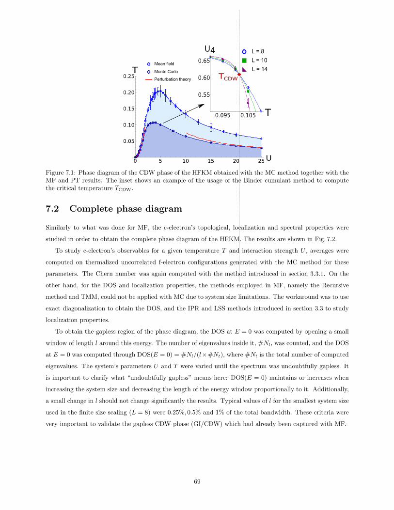
0 5 10 15 20 25U

0.05

0.10

0.15

0.20

0.25T

Mean field

Monte Carlo

Perturbation theory

0.095 0.105

0.55

0.60

0.65

L = 8

L = 10

L = 14TCDW

U4

T

Figure 7.1: Phase diagram of the CDW phase of the HFKM obtained with the MC method together with theMF and PT results. The inset shows an example of the usage of the Binder cumulant method to computethe critical temperature TCDW.

7.2 Complete phase diagram

Similarly to what was done for MF, the c-electron’s topological, localization and spectral properties were

studied in order to obtain the complete phase diagram of the HFKM. The results are shown in Fig. 7.2.

To study c-electron’s observables for a given temperature T and interaction strength U , averages were

computed on thermalized uncorrelated f-electron configurations generated with the MC method for these

parameters. The Chern number was again computed with the method introduced in section 3.3.1. On the

other hand, for the DOS and localization properties, the methods employed in MF, namely the Recursive

method and TMM, could not be applied with MC due to system size limitations. The workaround was to use

exact diagonalization to obtain the DOS, and the IPR and LSS methods introduced in section 3.3 to study

localization properties.

To obtain the gapless region of the phase diagram, the DOS at E = 0 was computed by opening a small

window of length l around this energy. The number of eigenvalues inside it, #Nl, was counted, and the DOS

at E = 0 was computed through DOS(E = 0) = #Nl/(l×#Nt), where #Nt is the total number of computed

eigenvalues. The system’s parameters U and T were varied until the spectrum was undoubtfully gapless. It

is important to clarify what “undoubtfully gapless” means here: DOS(E = 0) maintains or increases when

increasing the system size and decreasing the length of the energy window proportionally to it. Additionally,

a small change in l should not change significantly the results. Typical values of l for the smallest system size

used in the finite size scaling (L = 8) were 0.25%, 0.5% and 1% of the total bandwidth. These criteria were

very important to validate the gapless CDW phase (GI/CDW) which had already been captured with MF.

69

0 1 2 3 4 5U0.00

0.05

0.10

0.15

0.20

0.25

T

0.30

10100

T

1

TI GTI GI

GI/CDW

MI

MI/CDWTI/CDW

0 1 2 3 4 5 6U0.00

0.05

0.10

0.15

0.20

0.25

0.30T

GI MI

GTI/CDW

TI/CDW

GI/CDW

MI/CDW

IB/CDW

GTI

a b

Figure 7.2: Phase diagram of the HFKM in the interaction U - temperature T plane obtained with theMF (a) and MC (b) methods. The different phases follow: outside the charge density wave phase (CDW),topological insulator (TI) for small U , gapless topological insulator (GTI) and gapless insulator (GI) forintermediary U and Mott-like insulating phase (MI) for large U . Inside the CDW phase, phases with similarfeatures as their high temperature counterparts were found and the suffix “/CDW” was added.

Remarkably, if we compare the MC and MF phase diagrams (Fig. 7.2), the similarities are notorious.

Indeed, most of the phases obtained with MF were verified with MC. A summary of each phase is provided

below:

(CDW) Below the critical temperature TCDW, thin blue curve in Fig. 7.2b, the f-electrons start ordering

in a checkerboard-like pattern for which only one of the sublattices is occupied. Besides the trivial gapped

CDW phase (MI/CDW), a topological insulating phase with charge ordering (TI/CDW) exists along with a

peculiar region for which the c-electron’s spectrum is gapless inside the CDW phase (GI/CDW). Both these

phases had already been captured with MF. Regarding the GI/CDW phase, Fig. 7.3a shows the DOS inside

the MI/CDW and GI/CDW phases for U = 2.5 and L = 16, for which the transition between a gapped and

gapless regime can be clearly seen. An example of the DOS(E = 0) scaling inside the GI/CDW phase is

shown in Fig. 7.3d, for which it can be seen that the density of states is stabilized and does not scale to zero.

It is finally worth mentioning the agreement between the PT and MC results, meaning that the mapping

into the 2D Ising model based on a perturbative analysis up to second order provides a good description of

the order-disorder phase transition in the small and large U limits.

(TI and GTI) Gapped and gapless topological insulating phases, respectively. For T = 0, the f-electrons

only occupy one of the sublattices and therefore act as a staggered potential for the c-electrons. This means

that the topological insulating phase exists between U = 0 and U = 6√

3t2 ≈ 1, value at which the spectrum

gap closes and reopens signaling the topological phase transition. When we increase T , the topological

phase still exists and extends to larger U . This would be expected in that for the Haldane model with

binary disorder - the large temperature limit - the topological phase is only destroyed for U ≈ 2.7, meaning

there must be a temperature-driven topological phase transition for 1 < U < 2.7. The corresponding phase

transition curve is shown in Fig. 7.2, in red, and some of the Chern number curves used to obtain it are shown

in Fig. 7.4. This curve is very similar to the one obtained with MF (Fig. 5.8). However, it crosses the CDW

70

- 1 0 1E

0.04

0.08

0.12DOS

- 3 - 1 1 3E

0.1

0.2

DOS

- 2 0 2E

0.05

0.15DOS

GI - MIMI/CDW - GI/CDW TI - GTIa b c d

0.2 0.6 1.0

1

2

3

4x10-3

V0

DOS(E=0)

/V

Figure 7.3: a - c, Density of states for different points in the phase diagram: MI/CDW-(U, T ) = (2.5, 0.045),GI/CDW-(2.5, 0.085), TI-(1, 0.2), GTI-(2, 0.2), GI-(4, 0.2) and MI-(5, 0.2). The DOS plots are shown with aLorentzian broadening of width 0.01 and were obtained for L = 16. d, Finite size scaling of the DOS at E = 0for the point (2.5, 0.085) used in figure b. V0 corresponds to the volume of the smallest used system (withL = 8). The DOS(E = 0) was computed in an energy window corresponding to 1% of the full bandwidth forthe L = 8 system. This window was reduced proportionally to the system size for larger systems.

0.00 0.04 0.08 0.12T

0.2

0.6

1.0C

L=8L=10L=14

U=1.25

U=1.5

U=1.75

U=2

TI

1.0 1.5 2.0 2.5 3.0U

0.2

0.6

1.0Ca b

L=8L=10L=14

GTI GI

Figure 7.4: Chern number computed through averages on Monte Carlo configurations of f-electrons fordifferent system sizes, for fixed U (a) and T (b). These curves were used to obtain the topological phasetransition curve in Fig. 7.2.

phase transition curve for U ∼ 1.5 and it is smoother with respect to the MF results. This is not surprising

as the approximation used in the latter implies that the transition outside the CDW phase is equivalent

to the one obtained for the Haldane model with binary disorder, taking place for a fixed U , regardless the

temperature. The consequence was that, within the numerical accuracy of the results, it was not possible to

confirm the GTI/CDW phase which was already very narrow in the MF phase diagram. Besides this minor

difference, the topological phase extends into the gapless region of the phase diagram for higher temperatures

just like in MF. In Fig. 7.3b it can be seen that the topological gap existing in the TI phase is closed in the

GTI phase but we continue having C = 1 as shown in Fig. 7.4b. For the topological phase transition into the

TI phase, the gap closes and reopens at the phase transition curve. On the other hand, the transition from

the GTI into the GI phase is accompanied by the merging of the only two extended states that exist in the

spectrum and carry opposite Chern numbers (see discussion on localization in section 7.3).

71

(GI and MI) Gapless and Mott-like insulating phases, respectively. Increasing U from the GTI phase

leads to an interaction-driven topological phase transition into a trivial gapless insulating phase (GI). If we

continue increasing U , the c-electron spectrum acquires a Mott-like gap (MI). The DOS inside the GI and

MI phases is exemplified in Fig. 7.3c.

7.3 Localization properties

Studies on localization were also carried out inside the GI, GTI and GI/CDW phases. While for the MF

approach no deviations are expected from the universal behaviour of systems belonging to the unitary class

and subjected to uncorrelated disorder - every eigenstate is localized except for two extended states when

inside the topological phase - in the case of the exact model that does not have to be the case. Outside

the CDW phase, the correlations between f-electron occupations decay with a characteristic length ξ. For

distances larger than ξ, the disorder potential felt by the c-electrons becomes uncorrelated. These phases

smoothly extend to the high T limit, where disorder effects become equivalent to those of a binary quenched

potential and therefore, the type of disorder felt by c-electrons can be seen as uncorrelated, as in MF. However,

inside the CDW phase, we have long range order and the correlation length becomes infinite. One must then

carefully study localization properties in order to substantiate the insulating behaviour of the gapless phases.

The results obtained with the LSS and IPR methods are shown in Fig. 7.5. For the GI and GTI phases,

the LSS results show the presence of two extended states in the GTI phase and that these do not exist

anymore in the GI phase (Fig. 7.5a). The IPR was also computed for the GI phase (Fig. 7.5d) and although

it becomes smaller with system size away from E = 0, Fig. 7.5e shows that the scalings in this region manifest

the trend of converging to a constant when compared to the unit slope dashed red line associated with a

IPR ∝ V −1 scaling. This implies that all eigenstates are localized in agreement with the LSS results.

When we study localization in the GI/CDW phase, the story is different. Near E = 0, we clearly continue

having localized states as it can be seen in Figs. 7.5b,c and therefore the GI/CDW phase is insulating at half-

filling. Conversely, by again analysing these figures, we can see that a region in which the IPR scales with

V −1 for the used system sizes exists for −3 . E . −1 (and 1 . E . 3), suggesting the presence of extended

states in this region. However, the existence of these extended states is left as an open question. Even though

the IPR seems to scale with V −1 for the chosen system sizes, it may be the case that the eigenstates are

only weakly localized and deviations from the unit slope start appearing for larger system sizes. This region

of extended states is, nonetheless, a serious possibility. Inside the CDW phase, the c-electrons experience

something similar to a long range correlated disorder potential. This type of disorder was already shown to

be related with the appearence of regions of extended states [100, 101], and in particular in systems belonging

to the unitary class [102]. It is also important to note that if we use the LSS method inside the GI/CDW

phase, the obtained variances are larger than the expected value for extended states within the GUE. This

apparent disagreement with IPR results can be understood by noticing that Wigner distribution predictions

72

-3 -1 1 3E

0.05

0.15

IPR

L =8

L =10

L =12

L =14

L =16

- 1.2 - 0.6 0.0

- 5.0

- 3.5

- 2.0

logIPR

- 5.0

- 3.5

- 2.0- 1.2 - 0.6 0.0

log V0/V

logIPR

GI/CDW

GI

log V0/V

0.0

0.4

0.8

- 3 - 1 1 3

E

(σ/<s>)2

GTIGI

a

b

c

e

d

Figure 7.5: a, Variance of the LSS distributions obtained for different energies in the GI (GTI) phase for(U, T ) = (2, 0.1) ( = (3.5, 0.2) ) and L = 14. The thick red line corresponds to σ2/〈s〉2 = 0.178 which is thevariance of the Wigner distribution associated to extended states. The two extended states existing in theGTI phase are marked with arrows. b (e), Finite size scaling of the IPR with the system’s volume V for theenergies marked with the arrows in figure c (d), that shows the IPR for different sizes in the GI/CDW (GI)phase for (U, T ) = (2.5, 0.085) (= (3.5, 0.2) ). The IPR shown in figure c (d) for negative (positive) energiesis symmetric in E. The red dashed lines shown in figures b,e have a unit slope and indicate the scalingIPR ∼ V −1. The colors of the arrows that select specific energies in figure c (d) match the correspondingscaling curves in figure b (e).

are not expected to hold in this case due to the existence of correlations in f-electrons.

7.4 Finite temperature topological phases

DOS

- 3 - 2 - 1 0 1 2 30.0

0.1

0.2

0.3

0.4

E

0.0

0.2

0.4

0.6

0.8

- 2 0 2

E

(σ/<s>

)2

L=8

L=10

L=14

a b

(σ/<s>

)2

Figure 7.6: a, Variance of the level spacing distributions obtained for (U, T ) = (2, 0.1) for different systemsizes. b, Variance of the level spacing distributions and DOS for (U, T ) = (1.5, 0.06), a point inside theTI phase and very close to the topological phase transition curve. The arrows indicate the position ofthe extended states. The red line indicates the variance expected for extended states in the unitary class,σ2/〈s〉2 = 0.178.

73

To finish our analysis on the HFKM phase diagram, some comments should again be made on the robustness

of the obtained finite temperature topological phases. This discussion has already been addressed for the MF

results in section 5.4 and it is important to get back to it at this point.

Problems could arise from the transition between the MI/CDW and TI phases or from the transition

between the GI and GTI phases. In the latter, the transition between the GI and GTI phases continues

depending on the merge of the only two extended states existing inside the GTI phase. The condition for

the GTI phase to be robust is that kBT << ∆E, with ∆E being the energy separation of the extended

states If we are just slightly away from the phase transition curve, these extended states have already a large

separation in energy as it can be seen in Fig. 7.5a for the point (U, T ) = (2, 0.1) inside the GTI phase, for

which ∆E ≈ 4 while kBT = 0.1. Once we were only able to use small systems, different sizes were used for

this point in order to make sure that the position of the extended states did not vary. The results are shown

in Fig. 7.6a where it can be seen that this is the case.

Regarding the TI phase, the physics of Chern number carrying extended states continues to apply. Indeed,

just slightly above the topological phase transition, even though the gap is small, the extended states are

already widely separated in energy as it can be seen in Fig. 7.6b. Just like for the GTI phase, temperature

effects are not expected to suppress the TI phase even when close to the phase transition curve.

74

Chapter 8

Conclusion

In this thesis we unveiled the finite temperature phase diagram of the Haldane-Falicov-Kimball model. The

richness of this model allowed for the study of the interplay between topology, disorder and interactions at

finite temperatures.

Our road to the exact phase diagram started in chapter 4, where we studied how disorder effects influenced

the phase diagram of the Haldane model. We have seen that when disorder is applied on top of a finite

staggered potential, a typical phenomenon of topological Anderson insulators is observed: a disorder-driven

transition into a topological phase becomes possible. Interestingly, the case of binary disorder corresponds

to the high temperature limit of the HFKM, and in this limit, gapped and gapless topological insulating

phases were obtained for smaller U , followed by gapless and Mott-like gapped insulating phases for larger

U . The main question at the end of this chapter was what would happen to the topological phases once the

temperature was lowered.

In chapter 5 we used a mean field approach to take a first approximate look at the HFKM phase diagram.

At small temperatures, the f-electrons were found to order in a CDW phase for every interaction strength.

In particular, at T = 0, f-electrons act as a staggered potential for c-electrons. The consequence was that

c-electrons could be in a gapped TI phase with charge ordering for U up to a critical value Uc = 6√

3t2

at which the gap closed and reopened denoting a topological transition into a trivial gapped CDW phase.

Increasing the temperature from T = 0 lead to the discovery of two important phenomena: the emergence of a

region associated to gapless excitations in the c-electron spectrum for intermediate U , connecting to the high

temperature gapless phases; and the extension of the topological phase for U > 6√

3t2 and into the gapless

region of the phase diagram for high enough temperatures. The main consequences were the possibility of

temperature-driven phase transitions into topological phases and the existence of a gapless c-electron’s phase

coexisting with the CDW phase.

Still regarding mean field studies, an analysis on localization demonstrated the insulating character of

the gapless phases, associated with the localization of c-electrons’ eigenstates. These further showed that, as

expected, the finite-temperature topological phases were associated with two bulk extended states carrying

75

opposite Chern numbers. Just slightly away from the topological phase transition, these states were already

separated by an energy scale much larger than the temperature scale at which the finite temperature topo-

logical phases settled. These phases were then considered robust in the mean field scope. The mean field

approach provided an important way of predicting the possible phases of the HFKM. However, many new

questions arose, namely: how quantitatively accurate were the results; what was the fate of the gapless CDW

phase outside the mean field scope; and whether the finite temperature topological phases were still robust

in the exact model.

To address the still unanswered questions, perturbation theory was used to describe the small and large

U CDW phase transitions in chapter 6 and an extensive numerical analysis based on a Monte Carlo method

was carried out in chapter 7 to obtain the full exact phase diagram. The former was important to understand

the effective f-electron interactions mediated by c-electrons in the studied limits and to show that the mean

field results overestimated the CDW critical temperature. The latter unveiled the central results of the thesis.

Although the critical temperature of the CDW phase transition was overestimated with mean field, the Monte

Carlo and mean field phase diagrams showed remarkable similarities. In particular, the robustness of the

finite-temperature topological phases and the existence of a gapless insulating CDW phase were confirmed.

Furthermore, the exact phase diagram unveiled the possibility of spectral regions of extended and localized

states coexisting in the gapless CDW phase due to the long range nature of the interaction-induced disorder

potential.

Our findings suggest the existence of robust topological phases of matter at finite temperatures for systems

with a large mass unbalance between fermionic species, opening a new route for the study of temperature-

driven topological phases in systems of this type. Regarding the spectral properties inside the gapless CDW

phase, the coexistence of spectral regions of extended and localized states, if confirmed, would correspond

to one of the first examples of a many-body mobility edge in a strong interacting system and may suggest

similar phenomena to be present in the case of finite mass-ratio between electronic species. Indeed, it would

be interesting to investigate, as future work, how the phase diagrams obtained in this thesis evolve for a finite

mass-ratio between the fermionic species.

We finish by noticing that all the ingredients for the experimental realization of the HFKM with ultracold

atoms in optical lattices are separately available: there are recent implementations of mass unbalanced

fermions [103, 104], and the Haldane model has recently been successfully realized [105]. A direct verification

of our results should therefore be possible with state-of-the-art technology.

76

Relevant publications by the author

We provide below the list of submitted publications by the author relevant in the context of this thesis:

M. Goncalves, P. Ribeiro, E.V. Castro.

Dirac points merging and wandering in a model Chern insulator.

Eprint arXiv: 1809.08054.

We present a model for a Chern insulator on the square lattice with complex first and second neighbor hoppings

and a sublattice potential which displays an unexpectedly rich physics. Similarly to the celebrated Haldane

model, the proposed Chern insulator has two topologically non-trivial phases with Chern numbers ±1. As a

distinctive feature of the present model, phase transitions are associated to Dirac points that can move, merge

and split in momentum space, at odds with Haldane’s Chern insulator where Dirac points are bound to the

corners of the hexagonal Brillouin zone. Additionally, the obtained phase diagram reveals a peculiar phase

transition line between two distinct topological phases, in contrast to the Haldane model where such transition

is reduced to a point with zero sublattice potential. The model is amenable to be simulated in optical lattices,

facilitating the study of phase transitions between two distinct topological phases and the experimental analysis

of Dirac points merging and wandering.

M. Goncalves, P. Ribeiro, E.V. Castro.

The Haldane model under quenched disorder.


We study the half-filled Haldane model with Anderson and binary disorder and determine its phase diagram,

as a function of the Haldane flux and staggered sub-lattice potential, for increasing disorder strength. We

establish that disorder stabilizes topologically nontrivial phases in regions of the phase diagram where the

clean limit is topologically trivial. At small disorder strength, our results agree with analytical predictions

obtained using a first order self-consistent Born approximation, and extend to the intermediate and large

disorder values where this perturbative approach fails. We further characterize the phases according to their

gapless or gapped nature by determining the spectral weight at the Fermi level. We find that gapless topological

nontrivial phases are supported for both Anderson and binary disorder. In the binary case, we find a reentrant

topological phase where, starting from a trivial region, a topological transition occurs for increasing staggered

potential η, followed by a second topological transition to the trivial phase for higher values of η.

77

M. Goncalves, P. Ribeiro, R. Mondaini, E.V. Castro.

Temperature-driven gapless topological insulator.


We investigate the phase diagram of the Haldane-Falicov-Kimball model -- a model combining topology, in-

teractions and spontaneous disorder at finite temperatures. Using an unbiased numerical method, we map

out the phase diagram on the interaction--temperature plane. Along with known phases, we unveil an

insulating charge ordered state with gapless excitations and a temperature-driven gapless topological insulating

phase. Intrinsic - temperature generated - disorder, is the key ingredient explaining the unexpected behavior.

Our findings support the possibility of having temperature-driven topological phase transitions into gapped

and gapless topological insulating phases in systems with a large mass unbalance in fermionic species.

78

Bibliography

[1] Charles Kittel. Introduction to Solid State Physics. 2010.

[2] George Gruner and Stuart Brown. Charge and Spin Density Waves. Scientific American, (April):50–56,

1994.

[3] P. Fazekas. Lecture Notes on Electron Correlation and Magnetism. Series in modern condensed matter

physics. World Scientific, 1999.

[4] Miguel M. Ugeda, Aaron J. Bradley, Yi Zhang, Seita Onishi, Yi Chen, Wei Ruan, Claudia Ojeda-

Aristizabal, Hyejin Ryu, Mark T. Edmonds, Hsin Zon Tsai, Alexander Riss, Sung Kwan Mo, Dunghai

Lee, Alex Zettl, Zahid Hussain, Zhi Xun Shen, and Michael F. Crommie. Characterization of collective

ground states in single-layer NbSe 2. Nature Physics, 12(1):92–97, 2016.

[5] P. Drude. Zur Elektronentheorie der Metalle; II. Teil. Galvanomagnetische und thermomagnetische

Effecte. Annalen der Physik, 308(11):369–402, 1900.

[6] P. W. Anderson. Absence of diffusion in certain random lattices. Physical Review, 109(5):1492–1505,

1958.

[7] N. F. Mott and W. D. Twose. The theory of impurity conduction. Advances in Physics, 10(38):107–163,

1961.

[8] E. Abrahams, P. W. Anderson, D. C. Licciardello, and T. V. Ramakrishnan. Scaling theory of local-

ization: Absence of quantum diffusion in two dimensions. Physical Review Letters, 42(10):673–676,

1979.

[9] Patrick A. Lee and T. V. Ramakrishnan. Disordered electronic systems. Reviews of Modern Physics,

57(2):287–337, 1985.

[10] Fritz Haake. Quantum Signatures of Chaos. Springer, November 2000.

[11] Shinsei Ryu, Andreas P. Schnyder, Akira Furusaki, and Andreas W W Ludwig. Topological insulators

and superconductors: Tenfold way and dimensional hierarchy. New Journal of Physics, 12, 2010.

79

[12] J. M. Kosterlitz and D. J. Thouless. Ordering, metastability and phase transitions in two-dimensional

systems. Journal of Physics C: Solid State Physics, 6(7):1181–1203, 1973.

[13] E. H. Hall. On a New Action of the Magnet on Electric Currents. American Journal of Mathematics,

2(3):287, 1879.

[14] K. V. Klitzing, G. Dorda, and M. Pepper. New method for high-accuracy determination of the fine-

structure constant based on quantized hall resistance. Physical Review Letters, 45(6):494–497, 1980.

[15] L. Landau. Diamagnetism of Metals. Zeitschrift fur Physik, 64(9-10):629–637, 1930.

[16] D. J. Thouless, M. Kohmoto, M. P. Nightingale, and M. Den Nijs. Quantized hall conductance in a

two-Dimensional periodic potential. Physical Review Letters, 49(6):405–408, 1982.

[17] M. V. Berry. Quantal Phase Factors Accompanying Adiabatic Changes. Proceedings of the Royal

Society A: Mathematical, Physical and Engineering Sciences, 392(1802):45–57, 1984.

[18] Di Xiao, Ming Che Chang, and Qian Niu. Berry phase effects on electronic properties. Reviews of

Modern Physics, 82(3):1959–2007, 2010.

[19] F. D M Haldane. Model for a quantum hall effect without landau levels: Condensed-matter realization

of the ”parity anomaly”. Physical Review Letters, 61(18):2015–2018, 1988.

[20] Cui-Zu Chang, Jinsong Zhang, Xiao Feng, Jie Shen, Zuocheng Zhang, Minghua Guo, Kang Li, Yunbo

Ou, Pang Wei, Li-Li Wang, Zhong-Qing Ji, Yang Feng, Shuaihua Ji, Xi Chen, Jinfeng Jia, Xi Dai,

Zhong Fang, Shou-Cheng Zhang, Ke He, Yayu Wang, Li Lu, Xu-Cun Ma, and Qi-Kun Xue. Experi-

mental observation of the quantum anomalous Hall effect in a magnetic topological insulator. Science,

340(6129):167–70, 2013.

[21] L. Falicov and J. Kimball. Simple Model for Semiconductor-Metal Transitions: SmB 6 and

Transition-Metal Oxides. Physical Review Letters, 22(19):997–999, 1969.

[22] J. Hubbard. Electron Correlations in Narrow Energy Bands. Proceedings of the Royal Society A:

Mathematical, Physical and Engineering Sciences, 276(1365):238–257, 1963.

[23] A. H.. Castro Neto, N. M. R.. Peres, K. S.. Novoselov, A. K.. Geim, and F. Guinea. The electronic

properties of graphene. Reviews of Modern Physics, 81(1):109–162, 2009.

[24] Stephan Rachel and Karyn Le Hur. Topological insulators and mott physics from the hubbard inter-

action. Phys. Rev. B, 82:075106, Aug 2010.

[25] Youhei Yamaji and Masatoshi Imada. Mott physics on helical edges of two-dimensional topological

insulators. Phys. Rev. B, 83:205122, May 2011.

80

[26] Dong Zheng, Guang-Ming Zhang, and Congjun Wu. Particle-hole symmetry and interaction effects in

the kane-mele-hubbard model. Phys. Rev. B, 84:205121, Nov 2011.

[27] Christian Griset and Cenke Xu. Phase diagram of the kane-mele-hubbard model. Phys. Rev. B,

85:045123, Jan 2012.

[28] M. Hohenadler, Z. Y. Meng, T. C. Lang, S. Wessel, A. Muramatsu, and F. F. Assaad. Quantum phase

transitions in the kane-mele-hubbard model. Phys. Rev. B, 85:115132, Mar 2012.

[29] Johannes Reuther, Ronny Thomale, and Stephan Rachel. Magnetic ordering phenomena of interacting

quantum spin hall models. Phys. Rev. B, 86:155127, Oct 2012.

[30] Miguel A. N. Araujo, Eduardo V. Castro, and Pedro D. Sacramento. Change of an insulator’s topological

properties by a hubbard interaction. Phys. Rev. B, 87:085109, Feb 2013.

[31] Manuel Laubach, Johannes Reuther, Ronny Thomale, and Stephan Rachel. Rashba spin-orbit coupling

in the kane-mele-hubbard model. Phys. Rev. B, 90:165136, Oct 2014.

[32] M. Hohenadler, T. C. Lang, and F. F. Assaad. Correlation effects in quantum spin-hall insulators: A

quantum monte carlo study. Phys. Rev. Lett., 106:100403, Mar 2011.

[33] Shun-Li Yu, X. C. Xie, and Jian-Xin Li. Mott physics and topological phase transition in correlated

dirac fermions. Phys. Rev. Lett., 107:010401, Jun 2011.

[34] Christopher N. Varney, Kai Sun, Marcos Rigol, and Victor Galitski. Topological phase transitions for

interacting finite systems. Phys. Rev. B, 84:241105, Dec 2011.

[35] Roger S. K. Mong, Andrew M. Essin, and Joel E. Moore. Antiferromagnetic topological insulators.

Phys. Rev. B, 81:245209, Jun 2010.

[36] Chen Fang, Matthew J. Gilbert, and B. Andrei Bernevig. Topological insulators with commensurate

antiferromagnetism. Phys. Rev. B, 88:085406, Aug 2013.

[37] Tsuneya Yoshida, Robert Peters, Satoshi Fujimoto, and Norio Kawakami. Topological antiferromag-

netic phase in a correlated bernevig-hughes-zhang model. Phys. Rev. B, 87:085134, Feb 2013.

[38] S. Miyakoshi and Y. Ohta. Antiferromagnetic topological insulator state in the correlated bernevig-

hughes-zhang model. Phys. Rev. B, 87:195133, May 2013.

[39] S. Raghu, Xiao-Liang Qi, C. Honerkamp, and Shou-Cheng Zhang. Topological mott insulators. Phys.

Rev. Lett., 100:156401, Apr 2008.

[40] Jun Wen, Andreas Ruegg, C.-C. Joseph Wang, and Gregory A. Fiete. Interaction-driven topological

insulators on the kagome and the decorated honeycomb lattices. Phys. Rev. B, 82:075125, Aug 2010.

81

[41] Jan Carl Budich, Ronny Thomale, Gang Li, Manuel Laubach, and Shou-Cheng Zhang. Fluctuation-

induced topological quantum phase transitions in quantum spin-hall and anomalous-hall insulators.

Phys. Rev. B, 86:201407, Nov 2012.

[42] A. Dauphin, M. Muller, and M. A. Martin-Delgado. Rydberg-atom quantum simulation and chern-

number characterization of a topological mott insulator. Phys. Rev. A, 86:053618, Nov 2012.

[43] C. Weeks and M. Franz. Interaction-driven instabilities of a dirac semimetal. Phys. Rev. B, 81:085105,

Feb 2010.

[44] Lei Wang, Xi Dai, and X. C. Xie. Interaction-induced topological phase transition in the bernevig-

hughes-zhang model. EPL (Europhysics Letters), 98(5):57001, 2012.

[45] Andreas Ruegg and Gregory A. Fiete. Topological insulators from complex orbital order in transition-

metal oxides heterostructures. Phys. Rev. B, 84:201103, Nov 2011.

[46] Kai-Yu Yang, Wenguang Zhu, Di Xiao, Satoshi Okamoto, Ziqiang Wang, and Ying Ran. Possible

interaction-driven topological phases in (111) bilayers of lanio3. Phys. Rev. B, 84:201104, Nov 2011.

[47] Noel A. Garcıa-Martınez, Adolfo G. Grushin, Titus Neupert, Belen Valenzuela, and Eduardo V. Castro.

Interaction-driven phases in the half-filled spinless honeycomb lattice from exact diagonalization. Phys.

Rev. B, 88:245123, Dec 2013.

[48] Maria Daghofer and Martin Hohenadler. Phases of correlated spinless fermions on the honeycomb

lattice. Phys. Rev. B, 89:035103, Jan 2014.

[49] Johannes Motruk, Adolfo G. Grushin, Fernando de Juan, and Frank Pollmann. Interaction-driven

phases in the half-filled honeycomb lattice: An infinite density matrix renormalization group study.

Phys. Rev. B, 92:085147, Aug 2015.

[50] Sylvain Capponi and Andreas M. Lauchli. Phase diagram of interacting spinless fermions on the

honeycomb lattice: A comprehensive exact diagonalization study. Phys. Rev. B, 92:085146, Aug 2015.

[51] Kai Sun, Hong Yao, Eduardo Fradkin, and Steven A. Kivelson. Topological insulators and nematic

phases from spontaneous symmetry breaking in 2d fermi systems with a quadratic band crossing. Phys.

Rev. Lett., 103:046811, Jul 2009.

[52] Jorn W. F. Venderbos, Marco Manzardo, Dmitry V. Efremov, Jeroen van den Brink, and Carmine Or-

tix. Engineering interaction-induced topological insulators in a√

3×√

3 substrate-induced honeycomb

superlattice. Phys. Rev. B, 93:045428, Jan 2016.

[53] Han-Qing Wu, Yuan-Yao He, Chen Fang, Zi Yang Meng, and Zhong-Yi Lu. Diagnosis of interaction-

driven topological phase via exact diagonalization. Phys. Rev. Lett., 117:066403, Aug 2016.

82

[54] W. Zhu, Shou-Shu Gong, Tian-Sheng Zeng, Liang Fu, and D. N. Sheng. Interaction-driven spontaneous

quantum hall effect on a kagome lattice. Phys. Rev. Lett., 117:096402, Aug 2016.

[55] James M. Murray and Oskar Vafek. Renormalization group study of interaction-driven quantum anoma-

lous hall and quantum spin hall phases in quadratic band crossing systems. Phys. Rev. B, 89:201110,

May 2014.

[56] Oskar Vafek and Kun Yang. Many-body instability of coulomb interacting bilayer graphene: Renor-

malization group approach. Phys. Rev. B, 81:041401, Jan 2010.

[57] Jing Wang, Carmine Ortix, Jeroen van den Brink, and Dmitry V. Efremov. Fate of interaction-driven

topological insulators under disorder. Phys. Rev. B, 96:201104, Nov 2017.

[58] Tsuneya Yoshida, Satoshi Fujimoto, and Norio Kawakami. Correlation effects on a topological insulator

at finite temperatures. Phys. Rev. B, 85:125113, Mar 2012.

[59] Y-X Zhu, J He, C-L Zang, Y Liang, and S-P Kou. Magnetic topological insulators at finite temperature.

Journal of Physics: Condensed Matter, 26(17):175601, 2014.

[60] Yao-Hua Chen, Hsiang-Hsuan Hung, Guoxiong Su, Gregory A. Fiete, and C. S. Ting. Cellular dynamical

mean-field theory study of an interacting topological honeycomb lattice model at finite temperature.

Phys. Rev. B, 91:045122, Jan 2015.

[61] Damian Zdulski and Krzysztof Byczuk. Thermodynamic and topological phase diagrams of correlated

topological insulators. Phys. Rev. B, 92:125102, Sep 2015.

[62] A. Rivas, O. Viyuela, and M. A. Martin-Delgado. Density-matrix chern insulators: Finite-temperature

generalization of topological insulators. Phys. Rev. B, 88:155141, Oct 2013.

[63] P. Dziawa, B. J. Kowalski, K. Dybko, R. Buczko, A. Szczerbakow, M. Szot, E. Lusakowska, T. Balasub-

ramanian, B. M. Wojek, M. H. Berntsen, O. Tjernberg, and T. Story. Topological crystalline insulator

states in?Pb1?xSnxSe. Nature Materials, 2012.

[64] Masaru Onoda and Naoto Nagaosa. Quantized anomalous hall effect in two-dimensional ferromagnets:

Quantum hall effect in metals. Phys. Rev. Lett., 90:206601, May 2003.

[65] Masaru Onoda, Yshai Avishai, and Naoto Nagaosa. Localization in a quantum spin hall system. Phys.

Rev. Lett., 98:076802, Feb 2007.

[66] Jian Li, Rui-Lin Chu, J. K. Jain, and Shun-Qing Shen. Topological anderson insulator. Phys. Rev.

Lett., 102:136806, Apr 2009.

[67] C. W. Groth, M. Wimmer, A. R. Akhmerov, J. Tworzyd lo, and C. W. J. Beenakker. Theory of the

topological anderson insulator. Phys. Rev. Lett., 103:196805, Nov 2009.

83

[68] Juntao Song, Haiwen Liu, Hua Jiang, Qing-feng Sun, and X. C. Xie. Dependence of topological anderson

insulator on the type of disorder. Phys. Rev. B, 85:195125, May 2012.

[69] Ying Su, Y. Avishai, and X. R. Wang. Topological anderson insulators in systems without time-reversal

symmetry. Phys. Rev. B, 93:214206, Jun 2016.

[70] Christoph P. Orth, Tibor Sekera, Christoph Bruder, and Thomas L. Schmidt. The topological Anderson

insulator phase in the Kane-Mele model. Scientific Reports, 6, 2016.

[71] Nicholas Metropolis, Arianna W. Rosenbluth, Marshall N. Rosenbluth, Augusta H. Teller, and Ed-

ward Teller. Equation of state calculations by fast computing machines. Journal Chemical Physics,

21(6):1087–1092, 1953.

[72] David P. Landau and Kurt Binder. A guide to Monte-Carlo simulations in statistical physics. 2009.

[73] Helmut G Katzgraber. Introduction to Monte Carlo Methods. arXiv, pages 1–30, 2009.

[74] Maciej M. Maska and Katarzyna Czajka. Thermodynamics of the two-dimensional Falicov-Kimball

model: A classical Monte Carlo study. Physical Review B - Condensed Matter and Materials Physics,

74(3), 2006.

[75] U. Brandt and R. Schmidt. Exact results for the distribution of thef-level ground state occupation in

the spinless falicov-kimball model. Zeitschrift fur Physik B Condensed Matter, 63(1):45–53, Mar 1986.

[76] Tom Kennedy and Elliott H. Lieb. An itinerant electron model with crystalline or magnetic long range

order. Physica A: Statistical Mechanics and its Applications, 138(1-2):320–358, 9 1986.

[77] Martin Zonda, Pavol Farkasovsky, and Hana Cencarikova. Phase transitions in the three-dimensional

Falicov-Kimball model. Solid State Communications, 149(45-46):1997–2001, 2009.

[78] Andrey E. Antipov, Younes Javanmard, Pedro Ribeiro, and Stefan Kirchner. Interaction-Tuned An-

derson versus Mott Localization. Physical Review Letters, 117(14), 2016.

[79] V. M. Pereira, E. V. Castro, J. M. B. Lopes dos Santos, Faculdade De Ciencias, and Universidade Porto.

Disorder in the double exchange model. In Strongly Correlated Systems, Coherence and Entanglement,

pages 279–309. 2007.

[80] H.B. Callen, H.B. Callen, National Fund Raising Counsel of Australia. Research Division, and Wiley &

Sons. Thermodynamics and an Introduction to Thermostatistics. Wiley, 1985.

[81] H. Fehske, R. Schneider, and A. Weiße. Computational Many-Particle Physics. Lecture Notes in

Physics. Springer Berlin Heidelberg, 2007.

84

[82] Yi Fu Zhang, Yun You Yang, Yan Ju, Li Sheng, Rui Shen, Dong Ning Sheng, and Ding Yu Xing.

Coupling-matrix approach to the Chern number calculation in disordered systems. Chinese Physics B,

22(11), 2013.

[83] H. Ehrenreich, F. Seitz, and D. Turnbull. Solid State Physics. Number vol. 35 in Solid State Physics.

Elsevier Science, 1980.

[84] R. Haydock and C. M M Nex. Comparison of quadrature and termination for estimating the density

of states within the recursion method. Journal of Physics C: Solid State Physics, 17(27):4783–4789,

1984.

[85] C. Lanczos. An iteration method for the solution of the eigenvalue problem of linear differential and

integral operators. Journal of Research of the National Bureau of Standards, 45(4):255, 1950.

[86] K.H. Hoffmann and M. Schreiber. Computational Statistical Physics: From Billiards to Monte Carlo.

Springer Berlin Heidelberg, 2010.

[87] V I Osedelec. A multiplicative ergodic theorem: Lyapunov characteristic exponents for dynamical

systems. Trans. Mosc. Math. Soc., 19:197–231, 1968.

[88] Masaru Onoda, Yshai Avishai, and Naoto Nagaosa. Localization in a quantum spin hall system.

Physical Review Letters, 98(7), 2007.

[89] Emil Prodan. Disordered topological insulators: A non-commutative geometry perspective, 2011.

[90] Masaru Onoda and Naoto Nagaosa. Quantized Anomalous Hall Effect in Two-Dimensional Ferromag-

nets: Quantum Hall Effect in Metals. Physical Review Letters, 90(20):4, 2003.

[91] Eduardo V. Castro, M. Pilar Lopez-Sancho, and Marıa A.H. Vozmediano. Anderson localization

and topological transition in Chern insulators. Physical Review B - Condensed Matter and Materi-

als Physics, 92(8), 2015.

[92] Eduardo V. Castro, Raphael De Gail, M. Pilar Lopez-Sancho, and Marıa A.H. Vozmediano. Absence

of localization in a class of topological systems. Physical Review B, 93(24), 2016.

[93] Henrik Bruus and Karsten Flensberg. Many-body quantum theory in condensed matter physics - an

introduction. Oxford University Press, United States, 2004.

[94] P. Coleman. Introduction to Many-Body Physics. Cambridge University Press, 2015.

[95] A. Bobak, T. Lucivjansky, M. Zukovic, M. Borovsky, and T. Balcerzak. Theoretical study of the

frustrated ising antiferromagnet on the honeycomb lattice. In Acta Physica Polonica A, volume 131,

pages 636–638, 2017.

85

[96] Damian Zdulski and Krzysztof Byczuk. Thermodynamic and topological phase diagrams of correlated

topological insulators. Physical Review B - Condensed Matter and Materials Physics, 92(12), 2015.

[97] S.W. Lovesey. Topological Insulators and Topological Superconductors, by B. Andrei Bernevig with

Taylor L. Hughes. Contemporary Physics, 55(4):353–354, 2014.

[98] M. A. Ruderman and C. Kittel. Indirect exchange coupling of nuclear magnetic moments by conduction

electrons. Physical Review, 96(1):99–102, 1954.

[99] Eugene Kogan. RKKY Interaction in Gapped or Doped Graphene. Graphene, 02(01):8–12, 2013.

[100] M. Hilke. Noninteracting electrons and the metal-insulator transition in two dimensions with correlated

impurities. Phys. Rev. Lett., 91:226403, Nov 2003.

[101] F. A.B.F. De Moura, M. L. Lyra, F. Domınguez-Adame, and V. A. Malyshev. Coherent electron

dynamics in a two-dimensional random system with mobility edges. Journal of Physics Condensed

Matter, 19(5), 2007.

[102] D. Taras-Semchuk and K. B. Efetov. Influence of long-range disorder on electron motion in two dimen-

sions. Phys. Rev. B, 64:115301, Aug 2001.

[103] Gregor Jotzu, Michael Messer, Frederik Gorg, Daniel Greif, Remi Desbuquois, and Tilman Esslinger.

Creating state-dependent lattices for ultracold fermions by magnetic gradient modulation. Phys. Rev.

Lett., 115:073002, Aug 2015.

[104] Daniel Greif, Gregor Jotzu, Michael Messer, Remi Desbuquois, and Tilman Esslinger. Formation and

dynamics of antiferromagnetic correlations in tunable optical lattices. Phys. Rev. Lett., 115:260401,

Dec 2015.

[105] Gregor Jotzu, Michael Messer, Remi Desbuquois, Martin Lebrat, Thomas Uehlinger, Daniel Greif, and

Tilman Esslinger. Experimental realisation of the topological Haldane model. Nature, 515(7526):237–

240, jun 2014.

[106] Alan D. Sokal. Monte carlo methods in statistical mechanics: Foundations and new algorithms. 1996.

86

Appendix

87

Appendix A

Cubic spline method

A.1 Description of the method

We consider a set of points (xi, yi) with i = 1, ..., n+1 and a set of polynomials qj(x) with j = 1, ..., n defined

on each branch between points. For the cubic spline method, the polynomials can be written as

qi(x) = (1− t)yi + tyi+1 + t(1− t)[ai(1− t) + bit] , (A.1)

where

t ≡ t(x) = x−xi

xi+1−xi

ai = ki(xi+1 − xi)− (yi+1 − yi)

bi = −ki+1(xi+1 − xi) + yi+1 − yi

and the parameters ki are determined with the following set of linear equations:

2

x2 − x1k1 +

1

x2 − x1k2 = 3

y2 − y1

(x2 − x1)2(A.2)

ki−1

xi − xi−1+

(2

xi − xi−1+

2

xi+1 − xi

)ki +

ki+1

xi+1 − xi= 3

(yi − yi−1

(xi − xi−1)2+

yi+1 − yi(xi+1 − xi)2

)(A.3)

1

xn − xn−1kn−1 +

2

xn − xn−1kn = 3

yn − yn−1

(xn − xn−1)2. (A.4)

We now define the right hand side of the system of equations as the vector Y , to write

Mk = Y , (A.5)

88

where M is a matrix that only depends on xi. By solving the system, we obtain the ki coefficients and with

them, the qi polynomials.

A.2 Error propagation

A.2.1 Error in polynomials

Assuming that our data set is associated with errors δyi in the yi coordinate, we can start by finding how

these errors propagate into the polynomial errors δqi:

(δqi)2 = t2(δyi+1)2 + t2(δyi)

2 + t2(1− t)4(δai)2 + t4(1− t)2(δbi)

2 , (A.6)

where

(δai)2 = (xi+1 − xi)2(δki)

2 + (δyi+1)2 + (δyi)2)

(δbi)2 = (xi+1 − xi)2(δki+1)2 + (δyi+1)2 + (δyi)

2

To find δki we can solve the system A.5 for ki in terms of yi the former as linear combinations of the

latter. The error is then simply computed with quadratic error propagation

(δki)2 =

∑j

|ξij |2(δyj)2 ,

where ξij are the coefficients of the linear combination.

A.2.2 Error in x coordinate

We may be interested in finding the x coordinate corresponding to a y coordinate yP . Assuming that yP is

on branch i which is described by the polynomial qi we can find the x coordinate by solving the following

equation:

qi(x, xi, xi+1, yi, yi+1, bi) = yP ↔ x = x(yP , xi, xi+1, yi, yi+1, ai, bi) .

The error in the x coordinate is then given by

(δx)2 =

∣∣∣∣∣ ∂x∂yi∣∣∣∣∣2

(δyi)2 +

∣∣∣∣∣ ∂x

∂yi+1

∣∣∣∣∣2

(δyi+1)2 +

∣∣∣∣∣ ∂x∂ai∣∣∣∣∣2

(δai)2 +

∣∣∣∣∣ ∂x∂bi∣∣∣∣∣2

(δbi)2 . (A.7)

89

A.2.3 Error in intersection between polynomials

We want to solve the following equation for xint:

qi(xint, xi, xi+1, yi, yi+1, ai, bi) = q′i(xint, x′i, x′i+1, y

′i, y′i+1, a

′i, b′i) .

This equation can be easily solved as it involves the intersection of two cubic polynominals. The error is

then given by

(δxint)2 =

∣∣∣∣∣∂xint∂yi

∣∣∣∣∣2

(δyi)2 +

∣∣∣∣∣ ∂xint∂yi+1

∣∣∣∣∣2

(δyi+1)2 +

∣∣∣∣∣∂xint∂ai

∣∣∣∣∣2

(δai)2 +

∣∣∣∣∣∂xint∂bi

∣∣∣∣∣2

(δbi)2 +

∣∣∣∣∣∂xint∂y′i

∣∣∣∣∣2

(δy′i)2

+

∣∣∣∣∣ ∂xint∂y′i+1

∣∣∣∣∣2

(δy′i+1)2 +

∣∣∣∣∣∂xint∂a′i

∣∣∣∣∣2

(δa′i)2 +

∣∣∣∣∣∂xint∂b′i

∣∣∣∣∣2

(δb′i)2 .

(A.8)

90

Appendix B

Variational mean field for the HFKM

- analytical approach

B.1 Effective Hamiltonian

Instead of computing 〈H(nf)〉MF numerically through expression 3.8, we use an approximation for which

we consider every occupation number nif,A and nif,B to be fixed to their mean field average values. Formally,

this corresponds to the following approximation:

〈H(nAf,i, nBf,i)〉MF ≈ H(〈nAf,i〉MF , 〈nBf,i〉MF ) , (B.1)

where

〈nAf,i〉 = nFD(−ω) ≡ nA(ω)

〈nBf,i〉 = nFD(ω) ≡ nB(ω)

(nA + nB = 1) .

(B.2)

This approximation allows us to analitically compute 〈H(nf)〉MF . We first need to diagonalize

H(nf) ≡ H(nA, nB) (remember that e−βH(nf) = Tr[e−βH(nf)]):

H(nA, nB) ≡ HHald −U

2

∑i

c†i ci + U∑i∈A

c†i,Aci,AnA + U∑i∈B

c†i,Bci,BnB −UN

4(nA + nB)

= HHald −U

2

∑i

c†i ci +U

2(nA + nB)

∑i

(c†i,Aci,A + c†i,Bci,B) + Uδ∑i

(c†i,Aci,A − c†i,Bci,B)− UN

4

= HHald +Uδ

2

∑i

(c†i,Aci,A − c†i,Bci,B)− UN

4,

(B.3)

91

where N is the total number of sites and

HHald = −t∑〈i,j〉

c†i cj + t2∑〈〈i,j〉〉


ζic†i ci (B.4)

δ = nA − nB (B.5)

Therefore, in this approximation, the effect of the interaction is to add a staggered potential Uδ/2 to the

Haldane Hamiltonian. Introducing the Bloch basis c†i = 1√N

∑k e−ik·ric†k,α, with N being the total number

of unit cells and α = A(= B) if i belongs to sublattice A(B), we can write

H =∑k

Ψ†kh(k)Ψk −UN

4, (B.6)

with Ψk =[ck,A ck,B

]Tand

h(k) = C(k)I + d(k) · σ (B.7)

C(k) = 2t2 cos(φ)(cos(k · a1) + cos(k · a2) + cos(k · (a1 − a2)))

d1(k) = cos(k · a1) + cos(k · a2) + 1

d2(k) = sin(k · a1) + sin(k · a2)

d3(k) = η + Uδ/2 + 2t2 sin(φ)(sin(k · a1)− sin(k · a2)− sin(k · (a1 − a2)))

In the above expression we introduced the real space lattice vectors a1 = a2

[3√

3]T

and a2 =

a2

[3 −

√3]T

. In our case, φ = π/2 and therefore the eigenvalues are given by

ε±(k) = ±√d2

1(k) + d22(k) + d2

3(k) . (B.8)

In order to diagonalize the Hamiltonian B.6, we now introduce an unitary transformation U and define a

new set of operators Ψ′k =[αk βk

]in such a way that

H =∑k

Ψ†kU†Uh(k)U†UΨk −

UN

4=∑k

Ψ′†k

ε−(k) 0

0 ε+(k)

Ψ′k −UN

4

=∑k

(ε−(k)α†kαk + ε+(k)β†kβk

)− UN

4,

(B.9)

where ε± are given in expression B.8. Our aim is to compute 〈H(nA, nB)〉. In the Fock space spanned by

the states with occupation numbers nk,i, with i = α, β labelling eigenstates of the number operators α†kαk

and β†kβk, we have

92

e−βH(nA,nB) = Trc[e−βH ] = eβUN/4

∑nk,i

〈nk1,α, nk1,β , ...| e−βH(k) |nk,α, nk1,β , ...〉

= eβUN/4∑nk,α

〈nk1,α, nk2,α, ...| e−β∑

k′ ε−(k′)α†k′αk′ |nk1,α, nk2,α, ...〉

×∑nk,β

〈nk1,β , nk2,β , ...| e−β∑

k′ ε+(k′)β†k′βk′ |nk1,β , nk2,β , ...〉

= eβUN/4∏k

[(1 + e−βε−(k))(1 + e−βε+(k))

].

Therefore

H(nA, nB) = − 1

βln(Trc[e

−βH ])

= − 1

β

∑k∈1BZ,i=±

ln(1 + e−βεi(k))− UN

4

= − 1

β

V(2π)2

∑i=±

∫1BZ

d2k ln(1 + e−βεi(k))− UN

4.

(B.10)

If we now divide H(nA, nB) by the total number of sites N , we must take into account that V/N = A7/2,

where A7 = 3√

3a2/2 is the area of the honeycomb unit cell. The factor 2 comes from the fact that each

unit cell has 2 sites and therefore there are a total of N/2 unit cells with area A7. We finally have

H(nA, nB)/N = − 1

β

a2

(2π)2

3√

3

4

∑i=±

∫1BZ

d2k ln(1 + e−βεi(k))− U

4. (B.11)

B.1.1 Cross-check between analytical and numerical results

It is important to cross-check the results of the current approximation with the numerical results of section

5 in the cases that they must be the same. For T = 0 and for nA = 1 and nB = 0 they must yield the same

results as only one of the sublattices is occupied. For the numerical method used in section 5, the effective

Hamiltonian in expression 2.9 is reduced to

H(nf)/N → −U

4− 1

N

∑Ej<0

|Ej(nf)| . (B.12)

For the analytical method developed in this section, the Hamiltonian becomes

H(nA = 1, nB = 0)/N = −U4− 1

(2π)2

3√

3

4

∫1BZ

d2k ε−(k) , (B.13)

with ε−(k) defined in the previous section and the lattice constant a set to unity. The computations with

both methods are shown in Fig. B.1 in which we can see that for a small system of 12× 12 unit cells there is

already a very good agreement.

93

1 2 3 4 5U

- 2.5

- 2.0

- 1.5

- 1.0

H(nA = 1; nB = 0)/N

Analytical

Numerical

Figure B.1: Cross check between analytical and numerical results for T = 0 and the configuration corre-sponding to every sites of types A and B respectively occupied and empty.

1 2 3 4 5U

0.2

0.4

0.6

0.8

1.0

1.2T

CDW

Figure B.2: Phase diagram of the HFKM obtained through the variational mean field method under theapproximation in expression B.1.

B.2 Phase diagram

By computing the free energy functional F through expression 3.1, it was possible to obtain the phase diagram

for the current approximation, shown in Fig. B.2. The quadratic small U behaviour is already captured even

though the critical temperatures are clearly overestimated even when compared with the mean field results

in Fig. 5.2 for which an average on mean field configurations is performed to compute H. However, for

larger values of U the critical temperature starts growing linearly with the interaction strength meaning

that the approximation is not accurate to describe these regions of the phase diagram. The reason can be

simply understood in that the current approximation only considers long-range order which is important for

small U . However, for larger U , local electron correlations become very important meaning that the used

approximation becomes inaccurate. The results obtained in Fig. B.2 are very similar to the ones obtained in

Ref. [96] for the Hartree approximation.

94

Appendix C

Monte Carlo - Technical details

C.1 Errors and correlation times

The Monte Carlo Metropolis Hastings method introduced in section 3.2 samples a new state based on the

previous one. This means that consecutive states have some similarities leading to correlations between the

corresponding measurements. We are interested in computing averages of observables that we can estimate

by computing the average on a given Markov chain of length N :

O =1

N

N∑i=1

Oi . (C.1)

If the measurements were uncorrelated, the variance of this average would simply be σ2O = σ2

O/N , with

σ2O being the variance of single measurements. However, as we have emphasized, the measurements are

correlated and the variance will instead be given by [81]

σ2O =

σ2ON

+1

N2

∑i6=j

(〈OiOj〉 − 〈Oi〉〈Oj〉) . (C.2)

By using the interchangeability between indexes i and j and time translational symmetry (that must exist

in equilibrium), we can rearrange the second term in a more suitable way:

1

N2

∑i6=j

(〈OiOj〉 − 〈Oi〉〈Oj〉) =2

N2

N∑i=1

N∑j=i+1

(〈OiOj〉 − 〈Oi〉〈Oj〉)

=2

N

N∑k=1

(〈O1O1+k〉 − 〈O1〉〈O1+k〉)(

1− k

N

).

(C.3)

Notice that in the last step time translational symmetry implies N − k equal terms for each k and this is

accounted for in the term that multiplies on the right. If we now define the autocorrelation function A(k) as

A(k) = (〈O1O1+k〉 − 〈O1〉〈O1+k〉)/σ2O, we can write σ2

O as

95

σ2O =

σ2ON

2τO , (C.4)

where we define

τO =1

2+

N∑k=1

A(k)(

1− k

N

)(C.5)

as the correlation time. For large enough time separations k, A(k) decays exponentially and we can define

an exponential autocorrelation time τO,exp as as1

A(k)→ e−k/τO,exp(k →∞) . (C.6)

For sufficiently enough uncorrelated data, a given simultation must have N >> τO,exp and therefore

when the term proportional to k/N becomes important, A(k) will be already negligible and this term can be

omitted. The final expression for the correlation time τO becomes

τO =1

2+

N∑k=1

A(k) . (C.7)

We can identify σO as the error in O, εO. Large correlations are, of course, associated with a large τO

and this means that they increase the error with respect to an uncorrelated sample with the same size. In

fact, if we define Neff = N2τO

, we have

εO =σO√Neff

, (C.8)

which is the same expression as the one used for uncorrelated data, but with the sample size reduced from

N to Neff .

C.2 Numerical computation of correlation times

The correlation time τO could in principle be estimated by using the estimator

A(k) =1

N−k∑N−ki=1 (Oi − O)(Oi+k − O)

σ2O

(C.9)

for A(k). However, this estimator diverges as k approaches N . The usual approach is to cutoff the sum at

some value kmax. The cutoff must be chosen to be large enough to have a negligible bias in the computation

of τO, but small enough so that problems with the divergencies occurring for large k do not occur. The

standard approach is to stop the summation under the self-consistent condition kmax ∼ 6τO(kmax) [106].

1Notice that τO,exp 6= τO in general. Only if A(k) is a pure exponential will the two correlation times be similar up to smallcorrections for small τO.

96

C.3 Jackknife method for computing errors

The computation of correlation times must be carried out to conclude if we have sufficient uncorrelated data

in our measurements. However, a general method for computing errors of observables and quantities that are

nonlinear combinations of them would facilitate the error analysis. In this section we present the Jackknife

method used for this purpose.

We start by dividing a set of N measurements into NB bins of length l and defining the average in each

bin O(i)B as

O(i)B =

1

l

l∑j=1

O(i−1)l+j , (C.10)

with i = 1, · · · , NB . The Jackknife method consists of considering large blocks of data that contain all the

measurements except the ones from a given bin i. We can compute the average of a given Jackknife block in

a simple way in terms of the average on the removed bin as

OJi =NO − lO(i)

B

N − l, (C.11)

where i = 1, · · · , NB corresponds to the removed bin. The NB jackknife blocks are correlated because the

same data enters in NB − 1 of them and therefore the corresponding variance σ2J would correspond to an

unrealistic estimation of the error εO. To correct this effect, σ2J is multiplied by a factor (NB − 1)2 [81]. We

finally have

ε2O = (σJO)2 =NB − 1

NB

NB∑i=1

(OJi − O)2 . (C.12)

97

Appendix D

Connection between partition

function and fermionic propagator

through path integral formalism

We are interested in a quadratic Hamiltonian associated to actions that are quadratic in the fermionic fields.

In this case, we are in the class of Gaussian path integrals. Considering a quadratic Hamiltonian given in

terms of fermionic fields c†, c by H = c†αhαβcβ , the action can be written in terms of the Grassman variables

c, c as [94]

S =

∫ β

0

dτ cα(τ)(dτ + hαβ)cβ(τ) =

∫ β

0

dτ c(τ)(dτ + h)c(τ) , (D.1)

where τ = it is the imaginary time. We can introduce the Fourier transform into the Matsubara frequency

space:

c(τ) =1√β

∑n

c(iωn)eiωnτ , (D.2)

where ωn = (2n+ 1)π/β are the fermionic Matsubara frequencies. As the Hamiltonian is time-independent,

the action is diagonal in the Matsubara frequency subspace. If we extend the degrees of freedom of the

Grassman variables to incorporate the Matsubara frequencies, that is cα → cα,ωn , we can write the action in

the simple form

S =∑iωn

c(ωn)(−iωn + h)c(ωn) ≡ −cG−1c . (D.3)

We have defined G−1αβn = iωnδαβ − hαβ which is nothing more than the propagator of H. The product

in expression D.3 now incorporates the sum in the Matsubara frequencies. Using this result, the partition

98

function can be written as

Z =

∫D[c, c] exp

[− c(−G−1)c

]. (D.4)

This is a Gaussian integral that can readily be solved by using the following result of Grassman calculus

[94]:

∫D[ξ, ξ] exp[−ξAξ] = detA . (D.5)

Notice how this is different for bosonic fields for which the result would be (detA)−1. We finally get

Z = det(−G−1) . (D.6)

We must, however, not forget that the determinant is also taken in the Matsubara frequency space. If we

finally take the logarithm,

lnZ = ln det(−G−1) = Tr ln(−G−1) , (D.7)

we arrive at the result used in expression 6.3.

99

The phase diagram of the Haldane-Falicov-Kimball model · O diagrama de fases revelou tamb em uma...

Documents

Transcript of The phase diagram of the Haldane-Falicov-Kimball model · O diagrama de fases revelou tamb em uma...