The ®Mathematica Journal From Discrete to Continuous Spectra · 2019-11-19 · The ®Mathematica...

The Mathematica® Journal

From Discrete to Continuous SpectraExploring Spectral Distribution for Schrödinger Operators on Finite and Infinite IntervalsChristopher J. Winfield

We study the distribution of eigenspectra for operators of the form -y ''+ q(x) y with self-adjoint boundary conditions on both bounded and unbounded interval domains. With integrable potentials q, we explore computational methods for calculating spectral density functions involving cases of discrete and continuous spectra where discrete eigenvalue distributions approach a continuous limit as the domain becomes unbounded. We develop methods from classic texts in ODE analysis and spectral theory in a concrete, visually oriented way as a supplement to introductory literature on spectral analysis. As a main result of this study, we develop a routine for computing eigenvalues as an alternative to NDEigenvalues, resulting in fast approximations to implement in our demonstrations of spectral distribution.

■ IntroductionWe follow methods of the texts by Coddington and Levinson [1] and by Titchmarsh [2] (both

publicly available online via archive.org) in our study of the operator ℒ[y] =def -y ''+ q(x) yand the associated problem

ℒ[y] = λ y, (1)

where y ' =def dydx

on the interval ℐ = (0, ∞) with real parameter λ and boundary condition

sin(α) y(0) - cos(α) y ' (0) = 0 (2)

The Mathematica Journal 21 © 2019 Wolfram Media, Inc.

for fixed α, where 0 ≤ α < π. For continuous q ∈ L1(ℐ) (the set of absolutely integrablefunctions on ℐ), we study the spectral function ρ(λ) associated with (1) and (2) using twomain methods: First, following [1], we approximate ρ by step functions associated with

related eigenvalue problems on finite intervals Ib =def [0, b] for some sufficiently largepositive b; then, we apply asymptotic solution estimates along with an explicit formula for

spectral density dρdλ

[2]. For some motivation and clarification of terms, we recall a major

application: For certain solutions ψ(x, λ) of (1) and (2) and for any f ∈ L2(ℐ) (the set ofsquare-integrable functions on ℐ), a corresponding solution to (1) may take the form

f (x) = 0

+∞g(λ) ψ(x, λ) dρ(λ) =

0

+∞g(λ) ψ(x, λ)

dρ(λ)

dλdλ

where

g(λ) = ℐψ(x, λ) f (x) dx

(in a sense described in Theorem 3.1 of Chapter 9 [1]); here, g is said to be a spectral trans-form of f . By way of such spectral transforms, the differential operator ℒ may be repre-sented alternatively in the integral form

ℐψ(x, λ) ℒ[ f (x)] dx = λ g(λ),

where ρ induces a measure by which g ∈ L2(ℐ, dρ) (roughly, the set of square-integrablefunctions when integrated against dρ) and by which Parseval’s equality holds. Typicalexamples are the complete set of orthogonal eigenfunctions sin(n π x / b) : n = 1, 2, … forα = π

2 and the corresponding Fourier sine transform in the limiting case b = +∞ (cf.

Chapter 9, Section 1 [1]).For a fixed, large finite interval Ib, we consider the problem (1), (2) along with the bound-ary condition

cos(β) y(b) - sin(β) y ' (b) = 0, (3)(0 < β ≤ π), which together admit an eigensystem with correspondence

λk⟺ψk(x), k = 1, 2, …,

where the eigenvalues λk satisfying Δλk =def λk+1 - λk > 0 and where the eigenfunctionsψk(x) form a complete basis for L2(Ib). Since the associated spectral function ρb(λ) is a stepfunction with jumps at the various λk, we first estimate these λk by way of a related equa-tion arising from Prüfer (phase-space) variables and compute the corresponding jumpsΔρb(λk) = ;;ψk<<-2. Then, we use interpolation to approximate the continuous spectral function ρ(λ) using datafrom a case of large b at points λk and using

dρ(λ)

dλ λ=λk

≈Δρb(λk)

Δλk=

1

;;ψk<<2 (λk+1 - λk), (4)

imposing the condition ρ(λ) ≡ 0 for all λ ⩽ 0.

2 Christopher J. Winfield


We compare our results with those of a well-known formula [2] appropriate to our case onℐ, which we outline as follows: For fixed λ > 0, let ψ(x, λ) be the solution to (1) withboundary values

ψ(0, λ) = cos(α); ψ′(0, λ) = sin(α),

for which the asymptotic formula

ψ(x, λ) = A(λ) cos λ x + B(λ) sin λ x + o(1) (5)

holds as x → ∞. Then we have

dρ(λ)

dλ=

1

π λ A2(λ) + B2(λ)(6)

from Section 3.5 [2].

Finally, in the last section, we apply the above techniques to extend our study to operators onlarge domains [-b, b] and on ℝ, where spectral matrices take the place of spectral functionsas a matrix analog of spectral transforms on these types of intervals (cf. equation (5.5) [1]).The techniques are described in detail below, but it is of particular interest that our computa-tions uncover an interesting pattern in a discrete-spectrum case, as we are forced to refor-mulate our approach according to certain eigen-subspaces involved: our desired spectralapproximations are resolved by way of an averaging procedure in forming Riemann sums.

Various sections of Chapters 7–9 [1] (see also [3] and related articles) present useful intro-ductory discussion applied to material presented in this article; yet, with our focus on equa-tions (1)–(6), one may proceed given basic understanding of Riemann–Stieltjes integrationalong with knowledge of ordinary differential equations and linear algebra, commensuratewith (say) the use of Eigensystem and NDSolve.

■ An Eigenvalue EstimatorWe compute eigenvalues by first computing solutions θ(x, λ) on Ib ×ℝ to the following,arising from Prüfer variables (equation 2.4, Chapter 8 [1]):

w ' = cos2 w + (λ - q(x)) sin2 w; w(0) = arctany(0)

y ' (0)=

π

2- α. (7)

Here, tan(θ) = yy'

, where y is a nontrivial solution to (1), (2) and (3) and θ satisfies

θ(b, l)<l=λk = β + (k - 1) π (8)

From Discrete to Continuous Spectra 3


for positive integers k. We interpolate to approximate such solutions as an efficient means toinvert (8) in the variable l. And we use the following function on (7) throughout this article.

In[1]:= Pruefer[initial_, a_, b_, q_] := ParametricNDSolveValue[{y'[x] ⩵ Cos[y[x]]^2 + (l - q) Sin[y[x]]^2,y[a] ⩵ initial

}, y[b], {x, a, b}, {l}]

Consider an example with a = 0, b = 10, and potential q(x) = e-x for parameter l with0 ≤ l ≤ L, L = 5, in the case α = π

2, β = π.

In[2]:= α1 = Pi / 2;a1 = 0;b1 = 10;q1 = Exp[-x];solution1 = Pruefer[ArcTan[Sin[α1], Cos[α1]], a1, b1, q1];

We create an interpolation approximation for eigenvalues λk.

In[3]:= β1 = Pi;L1 = 5;θApproximation1 =

Interpolation[Table[{l, solution1[l]}, {l, 0, L1, .001}]];EigenvaluesApproximation1[k_] :=l /. NSolve[θApproximation1[l] ⩵ β1 + (k - 1) Pi, l][[1]]

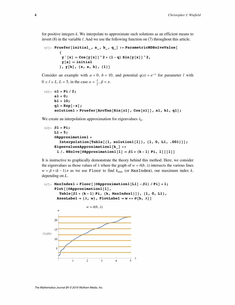
It is instructive to graphically demonstrate the theory behind this method. Here, we considerthe eigenvalues as those values of λ where the graph of w = θ(b, λ) intersects the various linesw = β + (k - 1) π as we use Floor to find kmax (or MaxIndex), our maximum index k,depending on L.

In[7]:= MaxIndex1 = Floor[(θApproximation1[L1] - β1) / Pi] + 1;Plot[{θApproximation1[l],

Table[β1 + (k - 1) Pi, {k, MaxIndex1}]}, {l, 0, L1},AxesLabel → {λ, w}, PlotLabel → w == θ[b, λ]]

Out[8]=

1 2 3 4 5λ

5

10

15

20

ww G θ(b, λ)



We choose these boundary conditions so that we may compare our results with thoseof NDEigenvalues applied to the corresponding problem (1) and (2) usingDirichletCondition.

In[9]:= operator[q_] := -y''[x] + q y[x];WolframEigenvalues =NDEigenvalues[{operator[q1], DirichletCondition[y[x] ⩵ 0, True]},y[x], {x, a1, b1}, MaxIndex1]

Out[10]= {0.121624, 0.450057, 0.963838,1.66557, 2.56019, 3.65123, 4.9415}

In[11]:= CoddingtonLevinsonEigenvalues =Table[Quiet@EigenvaluesApproximation1[k], {k, MaxIndex1}]

Out[11]= {0.121623, 0.45005, 0.963772,1.66522, 2.55891, 3.64748, 4.93221}

We now compare and contrast the methods in this case. The percent differences of thecorresponding eigenvalues are all less than 0.2%, even within our limits of accuracy.

In[12]:= Table[Abs[WolframEigenvalues[[n]] -

CoddingtonLevinsonEigenvalues[[n]]] /(Mean[{WolframEigenvalues[[n]],

CoddingtonLevinsonEigenvalues[[n]]}]), {n, MaxIndex1}]

Out[12]= 2.25034 × 10-6, 0.000015286, 0.0000677834,

0.000207569, 0.000500677, 0.00102788, 0.0018808

In contrast, our interpolation method allows some direct control of which eigenvalues are to becomputed, whereas NDEigenvalues (in the default setting) outputs a list up to 39 values,starting from the first. Moreover, our method admits nonhomogeneous boundary conditions,where NDEigenvalues admits only homogeneous conditions, Dirichlet or Neumann.

■ Spectral Density: Discrete Approximation

We proceed to build our approximate spectral density function dρdλ

for the problem (1) and(2) on ℐ with the same potential q as above. We compute eigenvalues likewise but now on alarger interval [0, b] for b = 150 and with nonhomogeneous boundary conditions, say givenby α = 3 π

4, β = π

4 (albeit ρ does not depend on β).

In[13]:= a2 = 0; b2 = 150; α2 = 3 Pi / 4; β2 = Pi / 4; L2 = 1; q2 = q1;



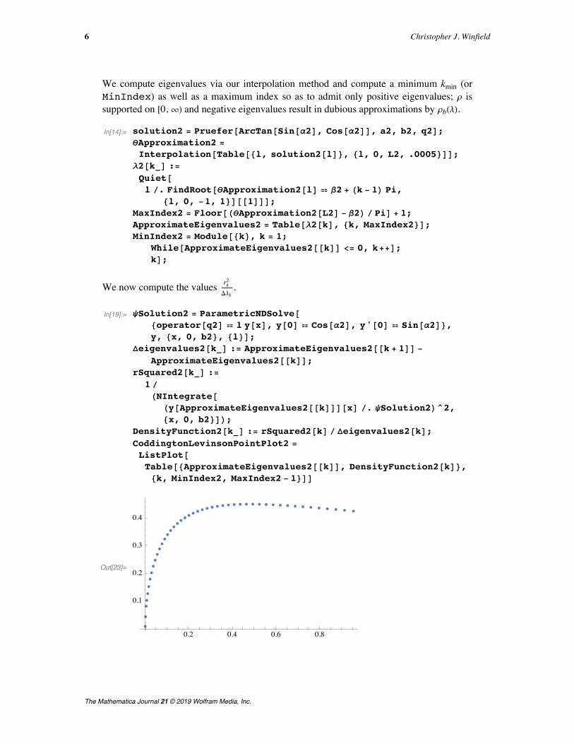
We compute eigenvalues via our interpolation method and compute a minimum kmin (orMinIndex) as well as a maximum index so as to admit only positive eigenvalues; ρ issupported on [0, ∞) and negative eigenvalues result in dubious approximations by ρb(λ).

In[14]:= solution2 = Pruefer[ArcTan[Sin[α2], Cos[α2]], a2, b2, q2];θApproximation2 =Interpolation[Table[{l, solution2[l]}, {l, 0, L2, .0005}]];

λ2[k_] :=Quiet[l /. FindRoot[θApproximation2[l] ⩵ β2 + (k - 1) Pi,

{l, 0, -1, 1}][[1]]];MaxIndex2 = Floor[(θApproximation2[L2] - β2) / Pi] + 1;ApproximateEigenvalues2 = Table[λ2[k], {k, MaxIndex2}];MinIndex2 = Module[{k}, k = 1;

While[ApproximateEigenvalues2[[k]] <= 0, k++];k];

We now compute the values rk2

Δλk.

In[19]:= ψSolution2 = ParametricNDSolve[{operator[q2] ⩵ l y[x], y[0] ⩵ Cos[α2], y'[0] ⩵ Sin[α2]},y, {x, 0, b2}, {l}];

Δeigenvalues2[k_] := ApproximateEigenvalues2[[k + 1]] -ApproximateEigenvalues2[[k]];

rSquared2[k_] :=1 /(NIntegrate[

(y[ApproximateEigenvalues2[[k]]][x] /. ψSolution2)^2,{x, 0, b2}]);

DensityFunction2[k_] := rSquared2[k] / Δeigenvalues2[k];CoddingtonLevinsonPointPlot2 =ListPlot[Table[{ApproximateEigenvalues2[[k]], DensityFunction2[k]},{k, MinIndex2, MaxIndex2 - 1}]]

Out[23]=

0.2 0.4 0.6 0.8

0.1

0.2

0.3

0.4



■ Fitting MethodWe now apply the method of [2] as outlined in equation (6). We use FindFit to includedata from an interval near the endpoint x = b that includes at least one half-period of theperiod of the fitting functions sin λ x and cos λ x.

In[24]:= FitTable2[k_] :=Table[{x, y[ApproximateEigenvalues2[[k]]][x] /.

ψSolution2},{x, b2 - Min[2 Pi / (Sqrt[ApproximateEigenvalues2[[k]]]),

b2 / 2], b2,Min[2 Pi / (Sqrt[ApproximateEigenvalues2[[k]]]), b2 / 2] /10}];

coefficient[k_] := FindFit[FitTable2[k],AA Cos[Sqrt[ApproximateEigenvalues2[[k]]] x] +BB Sin[Sqrt[ApproximateEigenvalues2[[k]]] x],

{AA, BB}, x];TInterpolation =

Interpolation[Table[{ApproximateEigenvalues2[[k]],

1 / (Pi Sqrt[ApproximateEigenvalues2[[k]]]((AA /. coefficient[k])^2 +

(BB /. coefficient[k])^2))},{k, MinIndex2, MaxIndex2}]];

TPlot = Plot[TInterpolation[x],{x, ApproximateEigenvalues2[[MinIndex2]],ApproximateEigenvalues2[[MaxIndex2]]}, PlotRange → Full,

PlotStyle → Green];

The function ApproximateEigenvalues may return non-numerical results among thefirst few, in which case we recommend that either b or L be readjusted or that MinIndex beset large enough to disregard such results.

We now compare our results of the discrete and continuous (asymptotic fit) spectraldensity approximations.



In[28]:= ShowCoddingtonLevinsonPointPlot2, TPlot,

AxesLabel → λ,Row[{d, ρ}]

Row[{d, λ}],

PlotLabel → "Spectral Density Approximations",Epilog →Inset[Framed[SwatchLegend[{Blue, Green},

{"Discrete case", "Asymptotic fit"}]],

Scaled[{.4, .6}]]

Out[28]=

0.2 0.4 0.6 0.8λ

0.1

0.2

0.3

0.4

dρ

dλ

Spectral Density Approximations

Discrete case

Asymptotic fit

We compare the results by plotting percent differences, all being less than 0.1%.

In[29]:= ListPlot[Table[{ApproximateEigenvalues2[[k]],

Abs[TInterpolation[ApproximateEigenvalues2[[k]]] -DensityFunction2[k]] /

Mean[{TInterpolation[ApproximateEigenvalues2[[k]]],DensityFunction2[k]}]}, {k, MinIndex2, MaxIndex2 - 1}],

AxesLabel → {λ, "%"},PlotLabel → "Percent Differences in Approximations"]

Out[29]=

0.2 0.4 0.6 0.8λ

0.02

0.04

0.06

0.08

0.10

%Percent Differences in Approximations



■ Check with Exact CalculationWe chose q as above because, in part, the solutions can be computed in terms of well-known BesselI (modified Bessel) functions. Replacing λ by l = λ + i ϵ, for λ, ϵ > 0, thesolutions are linear combinations of

BesselI2 i l , 2 e-x ,

BesselI-2 i l , 2 e-x .(9)

From asymptotic estimates (cf. equation 9.6.7 [4]), we see that the former is dominant andthe latter is recessive as x → +∞ when Im l > 0. Then, from Chapter 9 [1], equation 2.13and Theorem 3.1, we obtain the density function by computing

dρ(λ)

dλ=

-1

πlimϵ→0+

limb→+∞

φ(b, λ + i ϵ) / ψ(b, λ + i ϵ) =def -1

πlimϵ→0+

m( λ + i ϵ), (10)

where ψ(x, l) is a solution as above and φ(x, l) is a solution with boundary valuesφ(0, l) = sin(α), φ′(0, l) = -cos(α). (Here, m is commonly known as the Titchmarsh–Weylm-function.) In the following code, we produce the density function in exact form byreplacing functions from (9), the dominant by 1 and the recessive by 0, to compute theinside limit and thereafter simply allowing l = λ to be real.

In[30]:= ψExact2 =y[x] /.DSolve[{operator[q2] ⩵ l y[x], y[0] ⩵ Cos[α2],

y'[0] ⩵ Sin[α2]}, y, x][[1]];ϕExact2 =

y[x] /.DSolve[{operator[q2] ⩵ l y[x], y[0] ⩵ Sin[α2],

y'[0] ⩵ -Cos[α2]}, y, x][[1]];ratio2 = ϕExact2 / ψExact2

Out[32]= -BesselI-1 + 2 ⅈ l , 2 BesselI-2 ⅈ l , 2 ⅇ-x +

BesselI1 + 2 ⅈ l , 2 BesselI-2 ⅈ l , 2 ⅇ-x +

2 BesselI-2 ⅈ l , 2 ⅇ-x BesselI2 ⅈ l , 2 -

BesselI-1 - 2 ⅈ l , 2 BesselI2 ⅈ l , 2 ⅇ-x -

BesselI1 - 2 ⅈ l , 2 BesselI2 ⅈ l , 2 ⅇ-x -

2 BesselI-2 ⅈ l , 2 BesselI2 ⅈ l , 2 ⅇ-x

BesselI-1 + 2 ⅈ l , 2 BesselI-2 ⅈ l , 2 ⅇ-x +

BesselI1 + 2 ⅈ l , 2 BesselI-2 ⅈ l , 2 ⅇ-x -

2 BesselI-2 ⅈ l , 2 ⅇ-x BesselI2 ⅈ l , 2 -

BesselI-1 - 2 ⅈ l , 2 BesselI2 ⅈ l , 2 ⅇ-x -

BesselI1 - 2 ⅈ l , 2 BesselI2 ⅈ l , 2 ⅇ-x +

2 BesselI-2 ⅈ l , 2 BesselI2 ⅈ l , 2 ⅇ-x



In[33]:= Density2 =-1

Pi

Imratio2 /. BesselI2 ⅈ l , 2 ⅇ-x → 1,

BesselI-2 ⅈ l , 2 ⅇ-x → 0

Out[33]=

Im-BesselI-1-2 ⅈ l ,2-BesselI1-2 ⅈ l ,2-2 BesselI-2 ⅈ l ,2

-BesselI-1-2 ⅈ l ,2-BesselI1-2 ⅈ l ,2+2 BesselI-2 ⅈ l ,2

π

We likewise compare the exact formula for the continuous spectrum with the discreteresults, noting that the exact graph appears to essentially be the same as that obtained byour asymptotic fitting method (not generally expecting the fits to be accurate for small λ!).

In[34]:= ExactPlot2 = Plot[Density2, {l, 0, L2}, PlotRange → Full,PlotStyle → Black];

ShowCoddingtonLevinsonPointPlot2, ExactPlot2,

AxesLabel → λ,Row[{d, ρ}]

Row[{d, λ}], PlotLabel → "Spectral Density",

Epilog →Inset[Framed[SwatchLegend[{Blue, Black},

{"Discrete approximation", "Continuous, exact"}]],

Scaled[{.45, .65}]]

Out[35]=

0.2 0.4 0.6 0.8λ

0.1

0.2

0.3

0.4

dρ

dλ

Spectral Density

Discrete approximation

Continuous, exact



■ Extension to Unbounded Domains: A Proof of Concept

For the operator ℒ we now extend our study to large domains ℐb =def [-b, b] in the discrete-spectrum case and to the domain ℝ in the continuous-limit case. We choose an odd functionpotential of the form q(x) = c x e-r x for positive constants c, r. We focus on the spectraldensity associated with specific boundary values at x = 0 and an associated pair of solutionsto (1): namely, we consider expansions in the pair ϕ1(x, λ) and ϕ2(x, λ) such that

ϕ1(0, λ) = 1,ϕ1′ (0, λ) = 0,

ϕ2(0, λ) = 0,ϕ2′ (0, λ) = 1.

(11)

We apply the above computational methods to the analytical constructs from Chapter 5 [1]in both the discrete and continuous cases. First, for the discrete case, we compute spectralmatrices associated with self-adjoint boundary-value problems and the pair as in (11): Weestimate eigenvalues λk : k = 1, 2, … for an alternative two-point boundary-value problemon ℐb for (moderately) large b > 0 to compute the familiar jumps of the various componentsρi j;b(λ). These components induce measures that appear in the following form of Parseval’sequality for square-integrable functions f on ℐb (taken in a certain limiting sense):

gj(λ) = -b

bf (t) ϕ j(t, λ) dt,

-b

b; f (t)<2 dt =

-∞

∞i, j=1

2gi(λ) gj(λ) dρi j;b(λ) dλ

(real-valued case). Second, we compute the various densities as limits as b → +∞ bythe formulas

dρ jk(λ)

dλ= -

1

πIm Mjk(λ),

M11 =1

m- - m+,

M12 = M21 =1

2m- + m+ M11,

M22 = m- m+ M11,

(12)

where m+(λ) and m-(λ) are certain limits of m-functions, related to equation (10), but forour ODE problem on domains [0, +∞) and (-∞, 0], respectively. The densities are com-puted by procedures more elaborate than (6), as discussed later. Then, we compare resultsof the discrete case like in (4), approximating

dρi j(λ)

dλ λ=λk

≈Δρi j;b (λk)

Δλk. (13)



□ Discrete Case

After choosing (self-adjoint) boundary conditions (of which the limits ρi j happen to beindependent)

y(-b) = sin(α),y ' (-b) = cos(α),y(b) = sin(β),y ' (b) = cos(β),

(14)

on an interval ℐb, we estimate eigenvalues and compute coefficients r1;k, r2;k from thelinear combinations

hk(x) = r1;k ϕ1(x, λk) + r2;k ϕ2(x, λk)

for the associated orthonormal (complete) set of eigenfunctions hk; k = 1, 2, 3, ..., whereby

Δρi j;b(λk) = ri;k · rj;k

(real-valued case). Here, the functions hk(x) result by normalizing eigenfunctions ψk(x)satisfying (14) so that we obtain

r1;k = ψk(0);;ψk <<

,

r2;k = ψk ' (0);;ψk <<

.

We are ready to demonstrate. Let us choose q(x) = x e-5 ;x<, b = 50 π and α = π2

, β = 0(arbitrary). Much of the procedure follows as above, with minor modification, as weinclude ParametricNDSolveValue to obtain the values ψk(0) and ψk ' (0) (the nextresult may take around three minutes on a laptop).

In[36]:= L3 = 2; b3 = 50 Pi; a3 = -b3; α3 = Pi / 2; β3 = 0;q3 = x Exp[-5 Abs[x]];solution3 = Pruefer[ArcTan[Cos[α3], Sin[α3]], a3, b3, q3];ψsolution3 = ParametricNDSolve[

{operator[q3] ⩵ l y[x], y[a3] ⩵ Sin[α3], y'[a3] ⩵ Cos[α3]},y, {x, a3, b3}, {l}];

ψ3[l_, x_] := y[l][x] /. ψsolution3;θApproximation3 =

Quiet[Interpolation[Table[{l, solution3[l]},{l, 0, L3, .001}]]];

MaxIndex3 = Floor[(θApproximation3[L3] - β3) / Pi];λ3[n_] :=Quiet[l /. NSolve[θApproximation3[l] ⩵ β3 + (n - 1) Pi, l]][[1]]

eigenvalues3 = Table[λ3[n], {n, MaxIndex3}];



MinIndex3 = Module[{k},k = 1;While[eigenvalues3[[k]] <= 0, k++]; k

];NormSquared3[n_] := NIntegrate[ψ3[eigenvalues3[[n]], x]^2,

{x, a3, b3}];NormFactor3 = Table[NormSquared3[n],

{n, MinIndex3, MaxIndex3}];ψAtZero3 := ParametricNDSolveValue[

{operator[q3] ⩵ l y[x], y[a3] ⩵ Sin[α3], y'[a3] ⩵ Cos[α3]},y[0], {x, a3, b3}, {l}];

ψPrimeAtZero3 := ParametricNDSolveValue[{operator[q3] ⩵ l y[x], y[a3] ⩵ Sin[α3], y'[a3] ⩵ Cos[α3]},y'[0], {x, a3, b3}, {l}];

r1[n_] :=Quiet[Evaluate[ψAtZero3[eigenvalues3[[n]]]] /

Sqrt[NormFactor3[[n]]]];r2[n_] :=

Quiet[Evaluate[ψPrimeAtZero3[eigenvalues3[[n]]]] /Sqrt[NormFactor3[[n]]]];

We now approximate the density functions by plotting λk, Qi j;k where

Qi j;k =def Δρi j;b(λk) (λk+2 - λk) + Δρi j;b(λk+1) (λk+3 - λk+1) (15)

(for certain K ≤ kmax - 3) as we compute the difference quotients at the various jumps,over even and odd indices separately, and assign the corresponding sums Qi j;k to the

midpoints λk of corresponding intervals [λk, λk+1].

In[52]:= DifferenceQuotients11 =Table[{Mean[{eigenvalues3[[n]], eigenvalues3[[n + 1]]}],

r1[n]^2 / (eigenvalues3[[n + 2]] - eigenvalues3[[n]]) +r1[n + 1]^2 /(eigenvalues3[[n + 3]] - eigenvalues3[[n + 1]])},

{n, MinIndex3, MaxIndex3 - 3, 2}];DifferenceQuotients22 =

Table[{Mean[{eigenvalues3[[n]], eigenvalues3[[n + 1]]}],r2[n]^2 / (eigenvalues3[[n + 2]] - eigenvalues3[[n]]) +r2[n + 1]^2 /(eigenvalues3[[n + 3]] - eigenvalues3[[n + 1]])},

{n, MinIndex3, MaxIndex3 - 3, 2}];DifferenceQuotients12 =

Table[{Mean[{eigenvalues3[[n]], eigenvalues3[[n + 1]]}],r1[n] × r2[n] / (eigenvalues3[[n + 2]] - eigenvalues3[[n]]) +r1[n + 1] ×r2[n + 1] /(eigenvalues3[[n + 3]] - eigenvalues3[[n + 1]])},

{n, MinIndex3, MaxIndex3 - 3, 2}];DiscreteCasePlot =



In[52]:=

ListPlot[{DifferenceQuotients11, DifferenceQuotients22,DifferenceQuotients12},

PlotStyle → {Blue, Orange, Green}];

We give the plots below, in comparison with those of the continuous spectra, and give aheuristic argument in the Appendix as to why this approach works.

□ Continuous Case

First, we apply the asymptotic fitting method using the solutions ϕ1 and ϕ2. Here, we haveto compute full complex-valued formulas for the corresponding m-functions (cf. Section5.7 [2]) where a slight modification of the derivation of m+, via a change of variables anda complex conjugation, results in m- (See Appendix).

In[56]:= ϕ1solution = ParametricNDSolve[{Evaluate[operator[q3] ⩵ l y[x]], y[0] ⩵ 1, y'[0] ⩵ 0},y, {x, a3, b3}, {l}];

ϕ1[l_, x_] := y[l][x] /. ϕ1solution;ϕ2solution = ParametricNDSolve[

{Evaluate[operator[q3] ⩵ l y[x]], y[0] ⩵ 0, y'[0] ⩵ 1},y, {x, a3, b3}, {l}];

ϕ2[l_, x_] := y[l][x] /. ϕ2solution;Fitψ2Plus[l_] :=FindFit[Table[{x, ϕ2[l, x]},

{x, b3 - 2 Pi / Sqrt[l + 1], b3, 2 Pi / (15 Sqrt[l + 1])}],aa Cos[x Sqrt[l]] + bb Sin[x Sqrt[l]], {aa, bb}, x]

Fitψ1Plus[l_] :=FindFit[Table[{x, ϕ1[l, x]},

{x, b3 - 2 Pi / Sqrt[l + 1], b3, 2 Pi / (15 Sqrt[l + 1])}],cc Cos[x Sqrt[l]] + dd Sin[x Sqrt[l]], {cc, dd}, x]

Fitψ2Minus[l_] :=FindFit[Table[{x, ϕ2[l, x]},

{x, a3, a3 + 2 Pi / Sqrt[l + 1], 2 Pi / (15 Sqrt[l + 1])}],aa Cos[x Sqrt[l]] + bb Sin[x Sqrt[l]], {aa, bb}, x]

Fitψ1Minus[l_] :=FindFit[Table[{x, ϕ1[l, x]},

{x, a3, a3 + 2 Pi / Sqrt[l + 1], 2 Pi / (15 Sqrt[l + 1])}],cc Cos[x Sqrt[l]] + dd Sin[x Sqrt[l]], {cc, dd}, x]

APlus[l_] := aa /. Fitψ2Plus[l];BPlus[l_] := bb /. Fitψ2Plus[l];CPlus[l_] := cc /. Fitψ1Plus[l];DPlus[l_] := dd /. Fitψ1Plus[l];



AMinus[l_] := aa /. Fitψ2Minus[l];BMinus[l_] := bb /. Fitψ2Minus[l];CMinus[l_] := cc /. Fitψ1Minus[l];DMinus[l_] := dd /. Fitψ1Minus[l];

mPlus[l_] := -(CPlus[l] + I DPlus[l]) / (APlus[l] + I BPlus[l]);mMinus[l_] := -(CMinus[l] - I DMinus[l]) /

(AMinus[l] - I BMinus[l]);

dρ11[l_] := 1 / (Pi (mMinus[l] - mPlus[l]));dρ12[l_] := .5 (mPlus[l] + mMinus[l]) dρ11[l];dρ22[l_] := mPlus[l] × mMinus[l] × dρ11[l];

AsymptoticFit = Plot[{Im[dρ11[l]], Im[dρ22[l]], Im[dρ12[l]]},{l, eigenvalues3[[MinIndex3]], L3},PlotStyle → {Blue, Orange, Green}];

We now compare the result of the discrete and asymptotic fitting methods for the elements

Qi j =def dρij

dλ.

In[75]:= ShowAsymptoticFit, DiscreteCasePlot, Epilog → Inset[Text@Framed@Grid[{

{"", A11, A22, A12},{"Discrete", Style["●", Blue, 8],Style["●", Orange, 8], Style["●", Green, 8]},

{"Asymptotic", Style["———", Blue],Style["———", Orange], Style["———", Green]}

}, Alignment → {{Left, Center, Center}, Automatic}],Scaled[{0.7, 0.167}]],

PlotLabel → "Spectral Matrix Ai j - Various Methods",

ImageSize → {400, 300}

Out[75]=

0.5 1.0 1.5 2.0

-0.2

0.2

0.4

Spectral Matrix Qi j - Various Methods

&11 &22 &12

Discrete ● ● ●Asymptotic ——— ——— ———



■ AppendixWe have deferred some discussion on our use of Quiet, comparison of eigenvalue compu-tations, discrete eigenspace decomposition and Weyl m-functions to this section.

First, we have used Quiet to suppress messages warning that some solutions may not befound. From Chapter 8 [1], we expect unique solutions since the functions θ(b, ·) arestrictly increasing. We have also used Quiet to suppress various messages fromParametricNDSolve and other related functions regarding small values of q(x) to beexpected with short-range potentials and large domains.

Second, our formulation of Qi j and the midpoints λk as in (15) arises from a decompo-

sition of the eigenspace by even and odd indices. We motivate this decomposition by anexample plot of the values r1k · r2k, where the dichotomous behavior is quite pronounced,certainly for large k.

In[76]:= ListPlot[{Table[r1[n] × r2[n], {n, 1, MaxIndex3, 2}],Table[r1[n] × r2[n], {n, 2, MaxIndex3, 2}]},

Epilog →Inset[Framed[SwatchLegend[{Blue, Orange},

{"k odd", "k even"}]], Scaled[{.15, .15}]],PlotLabel → "The r1; k · r2; k Dichotomy",AxesLabel → {k, "r1; k · r2; k"}]

Out[76]=

10 20 30 40 50 60 70k

-0.004

-0.002

0.002

0.004

r1; k · r2; k

The r1; k ·r2; k Dichotomy

k odd

k even

We are thus inspired to compute the quotients over even and odd indices separately. Then,we consider, say, a relevant expression from Parseval’s equality: for appropriate Fouriercoefficients gi;k, i = 1, 2, associated with respective solutions ϕi, we write

∞

k=1

gi;k gj;k Δρi j;b(λk) =

k odd

gi;k gj;k Δρi j;b(λk) + gi;k+1 gj;k+1 Δρi j;b(λk+1) ≈ k odd

gi(λk) gj(λ

k) Qi j;k Δλk.



We suppose that λk+2 - λk ≈ 2 Δλk and gi;k ≈ gi;k+1 ≈ gi(λk) for the corresponding transforms

gi(λ) in the limit b → ∞. Of course, a rigorous argument is beyond the scope of this article.

Finally, we elaborate on the calculations of the m-functions m+ and m-: Given the asymp-totic expressions

ϕ1±(x, λ) = a±(λ) cos λ x + b±(λ) sin λ x + o(1),

ϕ2±(x, λ) = c±(λ) cos λ x + d±(λ) sin λ x + o(1),

as x → ±∞ (resp.), we follow Section 5.7 of [2], making changes as needed, with a modifi-cation via complex conjugation (l → λ - i ϵ, say) for m- to arrive at

m±(λ) = -c±(λ) ± i d±(λ)

a±(λ) ± i b±(λ)(resp.).

■ AcknowledgmentsThe author would like to thank the members of MAST for helpful and motivatingdiscussions concerning preliminary results of this work in particular and Mathematicacomputing in general.

■ References[1] E. A. Coddington and N. Levinson, Theory of Ordinary Differential Equations, New York:

McGraw-Hill, 1955. archive.org/details/theoryofordinary00codd.

[2] E. C. Titchmarsh, Eigenfunction Expansions Associated with Second-Order Differential Equa-tions, 2nd ed., London: Oxford University Press, 1962.archive.org/details/eigenfunctionexp0000titc.

[3] E. W. Weisstein. “Operator Spectrum” from MathWorld–A Wolfram Web Resource.mathworld.wolfram.com/OperatorSpectrum.html.

[4] M. Abramowitz and I. A. Stegun, eds., Handbook of Mathematical Functions with Formulas,Graphs, and Mathematical Tables, New York: Wiley, 1972.

C. Winfield, “From Discrete to Continuous Spectra,” The Mathematica Journal, 2019.https://doi.org/10.3888/tmj.21-3.

About the Author

C. Winfield holds an MS in physics and a PhD in mathematics and is a member of theMadison Area Science and Technology amateur science organization, based in Madison, WI.Christopher J. WinfieldMadison Area Science and Technology3783 US Hwy. 45Conover, WI [email protected]



The ®Mathematica Journal From Discrete to Continuous Spectra · 2019-11-19 · The ®Mathematica...

Documents

Transcript of The ®Mathematica Journal From Discrete to Continuous Spectra · 2019-11-19 · The ®Mathematica...