The Josephson Effect Jakob Blomgren 1998 Revised: Per Magnelind 2005

Purpose To describe the Josephson effect and show some consequences of it. To understand the workings of a SQUID (Superconducting QUantum Interference Device) and to demonstrate its features. Below is given a quite detailed discussion on various effects. Do not get lost in the derivations, but try to pick out the main results.

Introduction In 1962, B.D. Josephson analysed what happens at a junction between two closely spaced superconductors, separated by an insulating barrier. If the insulating barrier is thick, the electron pairs can not get through; but if the layer is thin enough (approximately 10 nm) there is a probability for electron pairs to tunnel. This effect later became known as 'Josephson tunnelling'. Besides displaying a broad range of interesting macroscopic quantum mechanical properties, the Josephson junction offers a vast survey of possible applications in analog and digital electronics, such as SQUID detectors, oscillators, mixers and amplifiers.

1 2

V

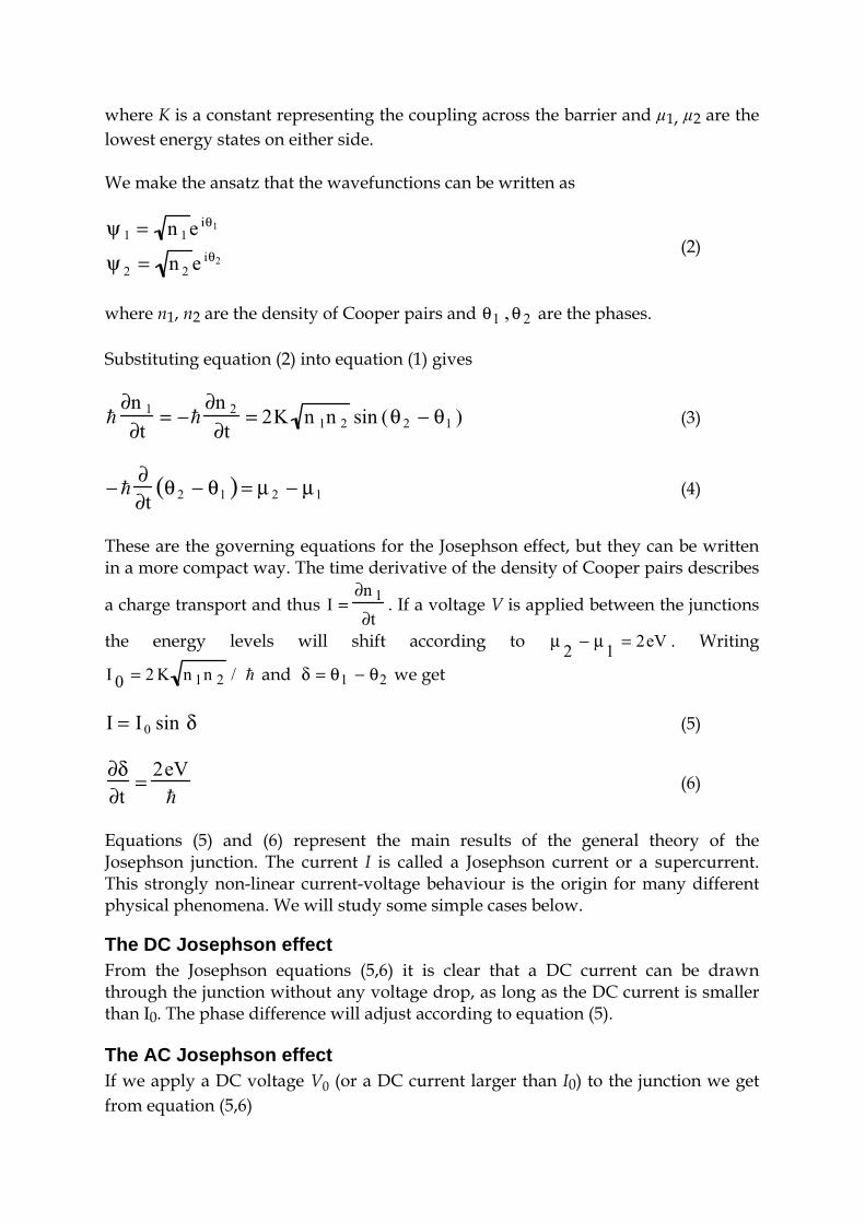
Ψ Ψ1 2 Figure 1. Two superconductors separated by a thin insulator

Theory of Josephson tunnelling In his famous lectures Feynman made a simplified derivation of the equations describing the Josephson tunnelling. We outline this derivation here. Suppose we have two superconductors that are connected by a thin layer of insulating material as shown in figure 1. We define Ψ1 and Ψ2 as the quantum mechanical wavefunction of the superconducting state in the left and the right superconductor, respectively. The dynamics of the two wavefunctions are then determined by the following coupled Schrödinger equations:

ih ∂ψ 1

∂t= µ 1ψ 1 + Kψ 2

ih ∂ψ 2

∂t= µ 2 ψ 2 + Kψ 1

(1)

where K is a constant representing the coupling across the barrier and µ1, µ2 are the lowest energy states on either side. We make the ansatz that the wavefunctions can be written as

ψ 1 = n 1 e iθ1

ψ 2 = n 2 e iθ2 (2)

where n1, n2 are the density of Cooper pairs and are the phases. θ1 ,θ 2 Substituting equation (2) into equation (1) gives

h

∂n 1

∂t= −h

∂n 2

∂t= 2K n 1n 2 sin (θ 2 − θ1 ) (3)

− h

∂∂t

θ 2 − θ1( )= µ 2 − µ1 (4)

These are the governing equations for the Josephson effect, but they can be written in a more compact way. The time derivative of the density of Cooper pairs describes

a charge transport and thus I =

∂n 1

∂t. If a voltage V is applied between the junctions

the energy levels will shift according to µ 2 − µ1 = 2eV . Writing

I 0 = 2 K n 1n 2 / h and we get δ = θ1 − θ2

I = I 0 sin δ (5)

∂δ∂t

= 2eVh

(6)

Equations (5) and (6) represent the main results of the general theory of the Josephson junction. The current I is called a Josephson current or a supercurrent. This strongly non-linear current-voltage behaviour is the origin for many different physical phenomena. We will study some simple cases below.

The DC Josephson effect From the Josephson equations (5,6) it is clear that a DC current can be drawn through the junction without any voltage drop, as long as the DC current is smaller than I0. The phase difference will adjust according to equation (5).

The AC Josephson effect If we apply a DC voltage V0 (or a DC current larger than I0) to the junction we get from equation (5,6)

I = I0 sin

2eV0

ht⎛

⎝ ⎜ ⎞ ⎠ ⎟

(7)

Thus when a voltage is applied, the Josephson current will oscillate at a frequency

f =

2eV0

h (8)

where 2e/h = 483.6 GHz/mV. The junctions capacitive and resistive properties, which is modelled in the Resistively and Capacitively Shunted Junction-model, now describes its DC characteristics.

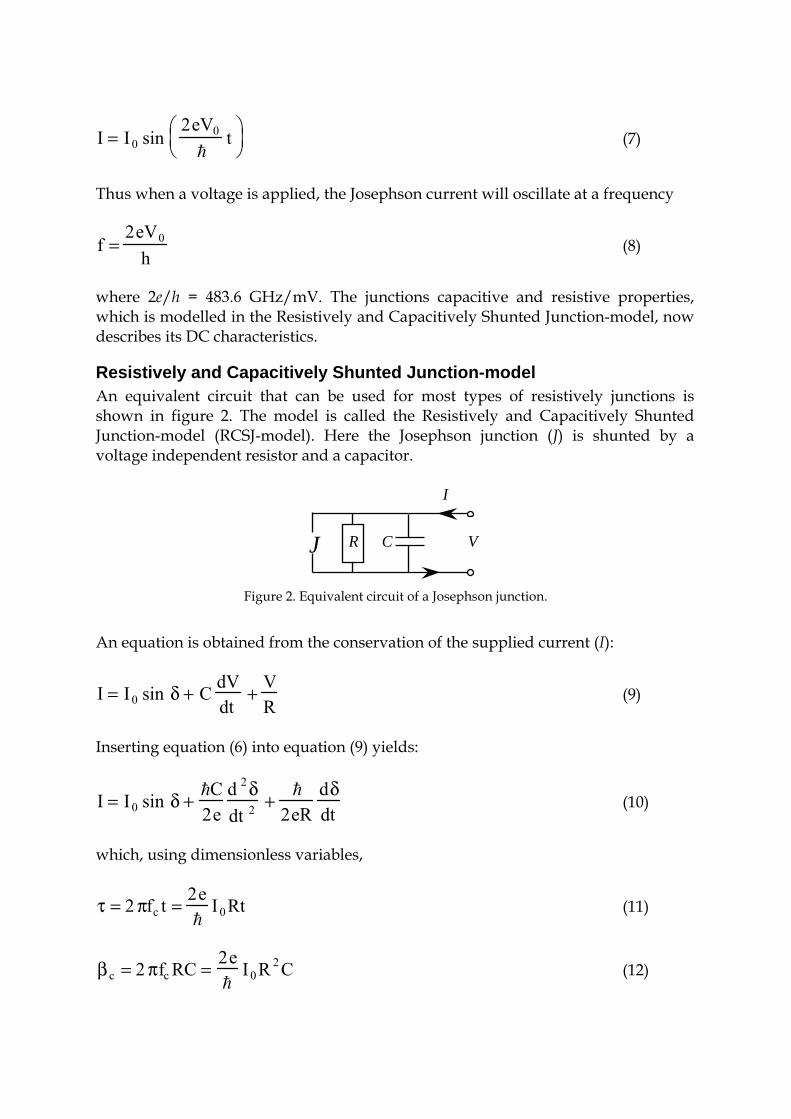
Resistively and Capacitively Shunted Junction-model An equivalent circuit that can be used for most types of resistively junctions is shown in figure 2. The model is called the Resistively and Capacitively Shunted Junction-model (RCSJ-model). Here the Josephson junction (J) is shunted by a voltage independent resistor and a capacitor.

J R C

I

V

Figure 2. Equivalent circuit of a Josephson junction.

An equation is obtained from the conservation of the supplied current (I):

I = I0 sin δ + C dV

dt+ V

R (9)

Inserting equation (6) into equation (9) yields:

I = I0 sin δ + hC

2ed 2 δdt 2 + h

2eRdδdt

(10)

which, using dimensionless variables,

τ = 2 πfc t = 2e

hI0 Rt (11)

β c = 2 πfc RC = 2e

hI0 R 2 C (12)

can be rewritten as:

i = sin δ + βc

d 2δdτ 2 + d δ

dτ (13)

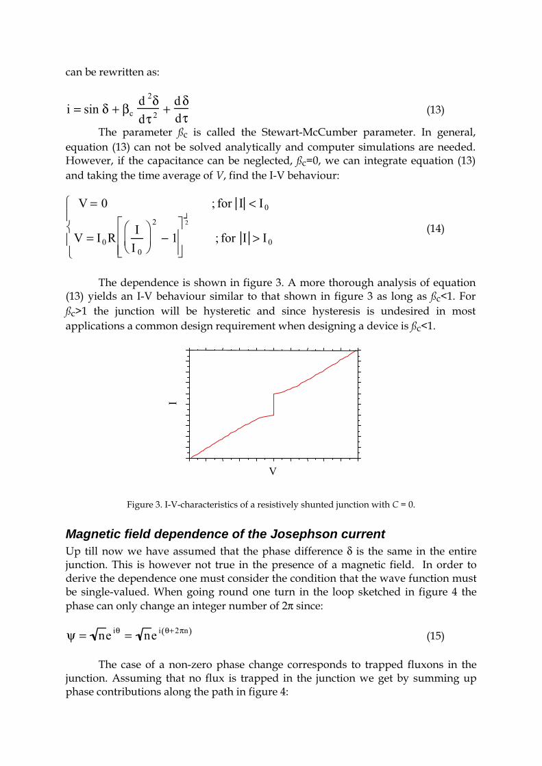
The parameter ßc is called the Stewart-McCumber parameter. In general, equation (13) can not be solved analytically and computer simulations are needed. However, if the capacitance can be neglected, ßc=0, we can integrate equation (13) and taking the time average of V, find the I-V behaviour:

V = 0 ; for I < I0

V = I0 R II 0

⎛

⎝ ⎜ ⎞

⎠ ⎟ 2

− 1⎡

⎣ ⎢ ⎢

⎤

⎦ ⎥ ⎥

12

; for I > I 0

⎧

⎨ ⎪

⎩ ⎪

(14)

The dependence is shown in figure 3. A more thorough analysis of equation (13) yields an I-V behaviour similar to that shown in figure 3 as long as ßc<1. For ßc>1 the junction will be hysteretic and since hysteresis is undesired in most applications a common design requirement when designing a device is ßc<1.

I

V

Figure 3. I-V-characteristics of a resistively shunted junction with C = 0.

Magnetic field dependence of the Josephson current Up till now we have assumed that the phase difference δ is the same in the entire junction. This is however not true in the presence of a magnetic field. In order to derive the dependence one must consider the condition that the wave function must be single-valued. When going round one turn in the loop sketched in figure 4 the phase can only change an integer number of 2π since:

ψ = ne iθ = ne i θ+2πn( ) (15) The case of a non-zero phase change corresponds to trapped fluxons in the junction. Assuming that no flux is trapped in the junction we get by summing up phase contributions along the path in figure 4:

∇ϕ • dl = 2 π

Φ 0A • dl∫ + m

2 e 2ρJ • dl∫ + δ x( )− δ(x + dx )∫ = 0 (16)

where A is the magnetic vector field. The integral in the first term on the right hand side is recognised as the total magnetic flux Φ in the loop. The integral in the second term on the right hand side can be neglected since it is only non-zero in the very small barrier region. Thus we are left with:

∂δ∂x

= 2 πΦ0

Φ = 2 eh

Bteff (17)

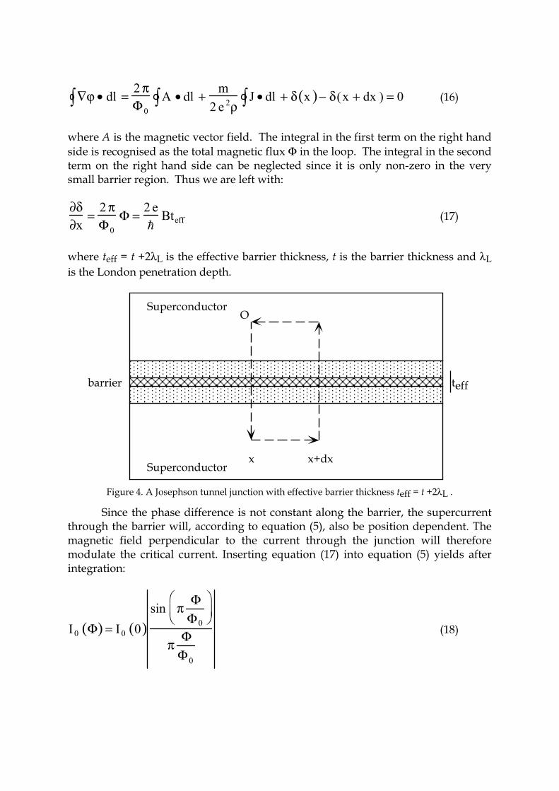
where teff = t +2λL is the effective barrier thickness, t is the barrier thickness and λL is the London penetration depth.

Superconductor O

barrier t eff

x x+dxSuperconductor

Figure 4. A Josephson tunnel junction with effective barrier thickness teff = t +2λL .

Since the phase difference is not constant along the barrier, the supercurrent through the barrier will, according to equation (5), also be position dependent. The magnetic field perpendicular to the current through the junction will therefore modulate the critical current. Inserting equation (17) into equation (5) yields after integration:

I 0 Φ( ) = I0 0( )sin π Φ

Φ0

⎛

⎝ ⎜ ⎞

⎠ ⎟

π ΦΦ0

(18)

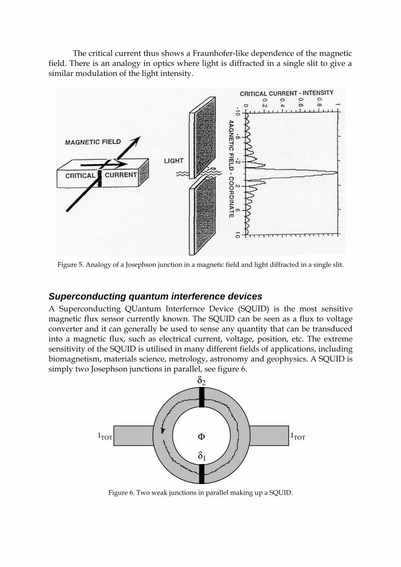
The critical current thus shows a Fraunhofer-like dependence of the magnetic field. There is an analogy in optics where light is diffracted in a single slit to give a similar modulation of the light intensity.

Figure 5. Analogy of a Josephson junction in a magnetic field and light diffracted in a single slit.

Superconducting quantum interference devices A Superconducting QUantum Interfernce Device (SQUID) is the most sensitive magnetic flux sensor currently known. The SQUID can be seen as a flux to voltage converter and it can generally be used to sense any quantity that can be transduced into a magnetic flux, such as electrical current, voltage, position, etc. The extreme sensitivity of the SQUID is utilised in many different fields of applications, including biomagnetism, materials science, metrology, astronomy and geophysics. A SQUID is simply two Josephson junctions in parallel, see figure 6.

ITOT ITOTΦ

δ1

δ2

Figure 6. Two weak junctions in parallel making up a SQUID.

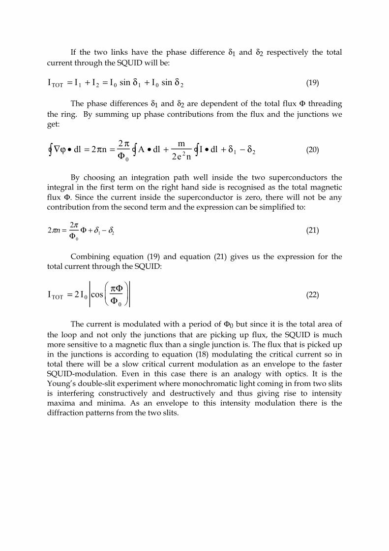
If the two links have the phase difference δ1 and δ2 respectively the total current through the SQUID will be:

ITOT = I1 + I2 = I0 sin δ1 + I0 sin δ 2 (19) The phase differences δ1 and δ2 are dependent of the total flux Φ threading the ring. By summing up phase contributions from the flux and the junctions we get:

∇ϕ • dl = 2πn = 2 π

Φ0A • dl∫ + m

2e 2 nI • dl∫ + δ1 − δ2∫ (20)

By choosing an integration path well inside the two superconductors the integral in the first term on the right hand side is recognised as the total magnetic flux Φ. Since the current inside the superconductor is zero, there will not be any contribution from the second term and the expression can be simplified to:

2πn =2πΦ0

Φ +δ 1 − δ2 (21)

Combining equation (19) and equation (21) gives us the expression for the total current through the SQUID:

ITOT = 2 I0 cos πΦ

Φ0

⎛

⎝ ⎜

⎞

⎠ ⎟ (22)

The current is modulated with a period of Φ0 but since it is the total area of the loop and not only the junctions that are picking up flux, the SQUID is much more sensitive to a magnetic flux than a single junction is. The flux that is picked up in the junctions is according to equation (18) modulating the critical current so in total there will be a slow critical current modulation as an envelope to the faster SQUID-modulation. Even in this case there is an analogy with optics. It is the Young’s double-slit experiment where monochromatic light coming in from two slits is interfering constructively and destructively and thus giving rise to intensity maxima and minima. As an envelope to this intensity modulation there is the diffraction patterns from the two slits.

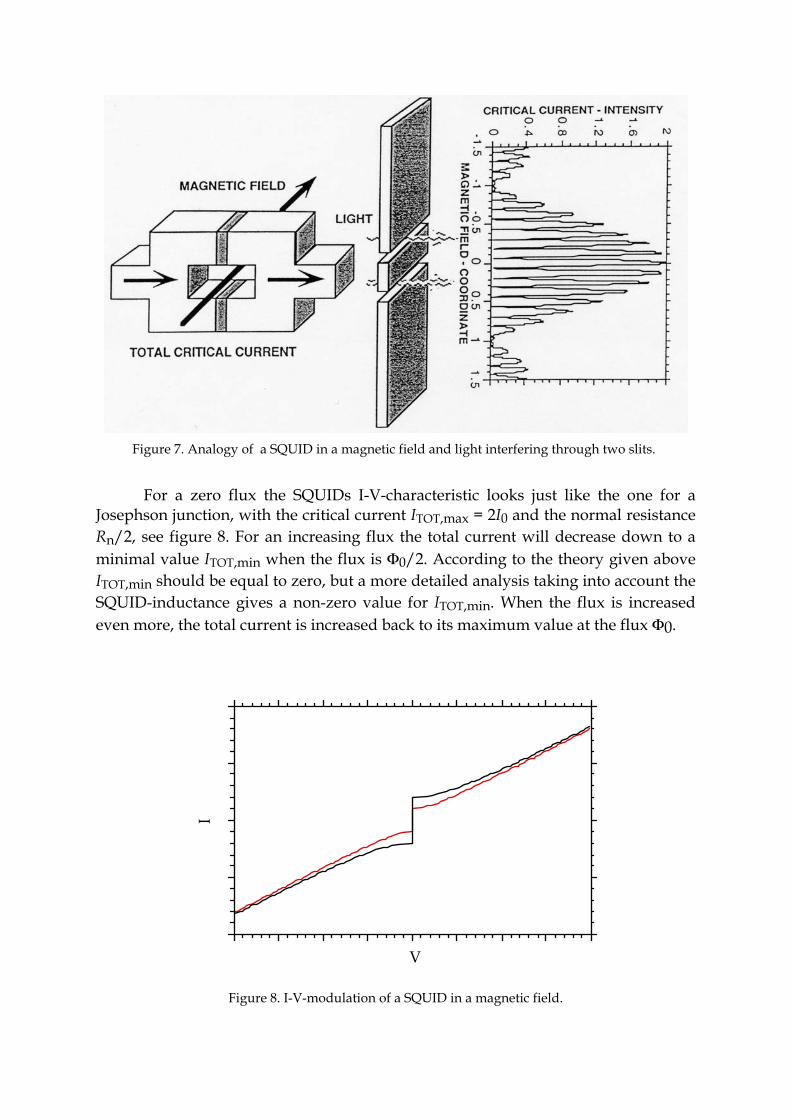
Figure 7. Analogy of a SQUID in a magnetic field and light interfering through two slits.

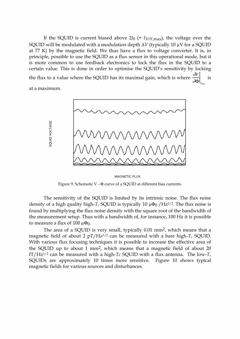
For a zero flux the SQUIDs I-V-characteristic looks just like the one for a Josephson junction, with the critical current ITOT,max = 2I0 and the normal resistance Rn/2, see figure 8. For an increasing flux the total current will decrease down to a minimal value ITOT,min when the flux is Φ0/2. According to the theory given above ITOT,min should be equal to zero, but a more detailed analysis taking into account the SQUID-inductance gives a non-zero value for ITOT,min. When the flux is increased even more, the total current is increased back to its maximum value at the flux Φ0.

I

V

Figure 8. I-V-modulation of a SQUID in a magnetic field.

If the SQUID is current biased above 2I0 (= ITOT,max), the voltage over the SQUID will be modulated with a modulation depth ∆V (typically 10 µV for a SQUID at 77 K) by the magnetic field. We thus have a flux to voltage converter. It is, in principle, possible to use the SQUID as a flux sensor in this operational mode, but it is more common to use feedback electronics to lock the flux in the SQUID to a certain value. This is done in order to optimise the SQUID’s sensitivity by locking

the flux to a value where the SQUID has its maximal gain, which is where ∂V∂Φ Ibias

is

at a maximum.

SQ

UID

VO

LTA

GE

MAGNETIC FLUX Figure 9. Schematic V - Φ curve of a SQUID at different bias currents.

The sensitivity of the SQUID is limited by its intrinsic noise. The flux noise

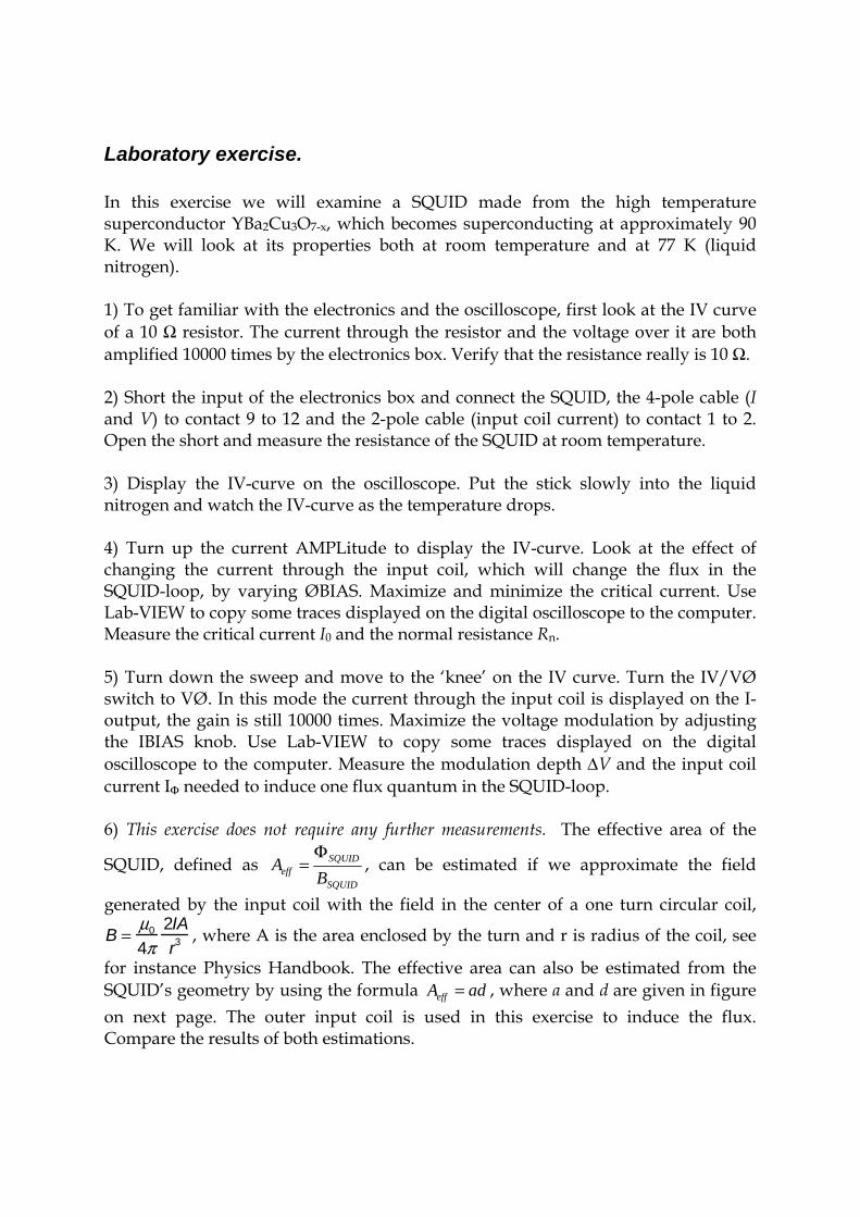
density of a high quality high-Tc SQUID is typically 10 µΦ0 /Hz1/2. The flux noise is found by multiplying the flux noise density with the square root of the bandwidth of the measurement setup. Thus with a bandwidth of, for instance, 100 Hz it is possible to measure a flux of 100 µΦ0. The area of a SQUID is very small, typically 0.01 mm2, which means that a magnetic field of about 2 pT/Hz1/2 can be measured with a bare high-Tc SQUID. With various flux focusing techniques it is possible to increase the effective area of the SQUID up to about 1 mm2, which means that a magnetic field of about 20 fT/Hz1/2 can be measured with a high-Tc SQUID with a flux antenna. The low-Tc SQUIDs are approximately 10 times more sensitive. Figure 10 shows typical magnetic fields for various sources and disturbances.

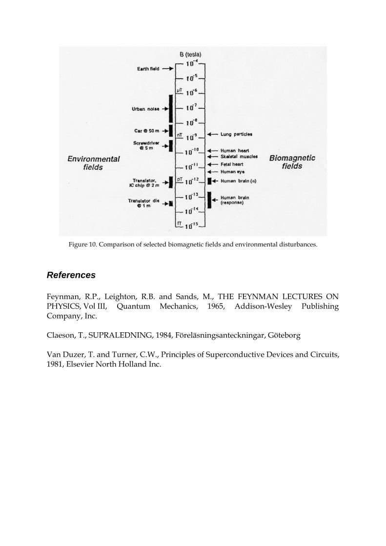
Figure 10. Comparison of selected biomagnetic fields and environmental disturbances.

References Feynman, R.P., Leighton, R.B. and Sands, M., THE FEYNMAN LECTURES ON PHYSICS, Vol III, Quantum Mechanics, 1965, Addison-Wesley Publishing Company, Inc. Claeson, T., SUPRALEDNING, 1984, Föreläsningsanteckningar, Göteborg Van Duzer, T. and Turner, C.W., Principles of Superconductive Devices and Circuits, 1981, Elsevier North Holland Inc.

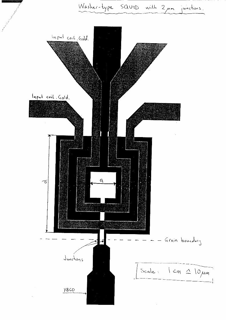
Laboratory exercise. In this exercise we will examine a SQUID made from the high temperature superconductor YBa2Cu3O7-x, which becomes superconducting at approximately 90 K. We will look at its properties both at room temperature and at 77 K (liquid nitrogen). 1) To get familiar with the electronics and the oscilloscope, first look at the IV curve of a 10 Ω resistor. The current through the resistor and the voltage over it are both amplified 10000 times by the electronics box. Verify that the resistance really is 10 Ω. 2) Short the input of the electronics box and connect the SQUID, the 4-pole cable (I and V) to contact 9 to 12 and the 2-pole cable (input coil current) to contact 1 to 2. Open the short and measure the resistance of the SQUID at room temperature. 3) Display the IV-curve on the oscilloscope. Put the stick slowly into the liquid nitrogen and watch the IV-curve as the temperature drops. 4) Turn up the current AMPLitude to display the IV-curve. Look at the effect of changing the current through the input coil, which will change the flux in the SQUID-loop, by varying ØBIAS. Maximize and minimize the critical current. Use Lab-VIEW to copy some traces displayed on the digital oscilloscope to the computer. Measure the critical current I0 and the normal resistance Rn. 5) Turn down the sweep and move to the ‘knee’ on the IV curve. Turn the IV/VØ switch to VØ. In this mode the current through the input coil is displayed on the I-output, the gain is still 10000 times. Maximize the voltage modulation by adjusting the IBIAS knob. Use Lab-VIEW to copy some traces displayed on the digital oscilloscope to the computer. Measure the modulation depth ∆V and the input coil current IΦ needed to induce one flux quantum in the SQUID-loop. 6) This exercise does not require any further measurements. The effective area of the

SQUID, defined as SQUID

SQUIDeff B

AΦ

= , can be estimated if we approximate the field

generated by the input coil with the field in the center of a one turn circular coil,

B =µ0

4π2IAr3 , where A is the area enclosed by the turn and r is radius of the coil, see

for instance Physics Handbook. The effective area can also be estimated from the SQUID’s geometry by using the formula , where a and d are given in figure on next page. The outer input coil is used in this exercise to induce the flux. Compare the results of both estimations.

adAeff =