The Intranational Business Cycle:

Evidence from Japan

by

Michael Artis, Manchester University and CEPR*†

and

Toshihiro Okubo, Manchester University**

January 2008

Abstract: This paper studies the intranational business cycle – that is the set of regional

(prefecture) business cycles – in Japan. One reason for choosing to examine the

Japanese case is that long time series and relatively detailed data are available. A

Hodrick-Prescott filter is applied to identify the cycles in annual data from 1955 to 1995

and bilateral cross-correlation coefficients are calculated for all the pairs of prefectures.

Comparisons are made with similar sets of bilateral cross correlation coefficients

calculated for the States of the US and for the member countries of a “synthetic Euro

Area”. The paper then turns to an econometric explanation of the cross-correlation

coefficients (using Fisher’s z-transform), in a panel data GMM estimation framework.

An augmented gravity model provides the basic model for the investigation, whilst the

richness of the data base also allows for additional models to be represented.

JEL Classification : E32, F41, R11

Keywords: Intranational business cycle, Hodrick-Prescott filter, Optimal Currency Area,

Gravity Model, Market potential, Heckscher Ohlin theorem.

*†Professor of Economics, Manchester Regional Economics Centre, Institute for

Political and Economic Governance, Manchester University, Oxford Rd., Manchester,

M13 9PL. E-mail: Michael.Artis@manchester.ac.uk

**Research Associate, Manchester Regional Economics Centre, Institute for Political

and Economic Governance, Manchester University, Oxford Rd., Manchester, M13 9PL.

E-mail: Toshihiro.Okubo@manchester.ac.uk

†Denotes corresponding author Acknowledgments: The authors are grateful to Tommaso Proietti, Len Gill, George

Chouliarakis, Pierre Picard, Denise Osborn and participants at seminars in Kobe and

Manchester Universities for their advice along the way. They are also grateful to Kyoji Fukao

and Hyeog Ug Kwon for providing data sets.

2

1. Introduction

The intranational business cycle is just the set of business cycles that characterize

the regions of a country (or, as we shall also use the term, the constituent countries of a

currency union). Although less commonly studied1, analysis of the intranational business

cycle offers a useful benchmark for comparison with the results obtained from

international business cycle analysis. For example, issues of adjustment and of

consumption-risk spreading, and more generally many of the predictions of Real

Business Cycle (RBC) theory which have been investigated at the international level can

also be analyzed at the intranational level – often with different results. Those

differences provide a challenge for explanation. Intranational cycles have also been

studied in the past in connection with propositions in the optimal currency area (OCA)

literature, particularly with respect to risk-sharing mechanisms and the like.2 In this last

respect Wincoop (1995) and Iwamoto and Wincoop (2000) offer leading examples.

Naturally the OCA perspective is not the only one that should be important in

studies of the intranational cycle. Indeed, as amplified below, many of the variables that

determine or are alleged to determine the degree of international business cycle

convergence, can have no salience in the study of the intranational context. We have

chosen to investigate the intranational business cycle in Japan. An advantage of choosing

Japan is that a relatively lengthy time series and reasonably comprehensive set of

regional accounts and factor endowments exists for Japan’s 47 prefectures.3 Furthermore,

the regional context of the intranational cycle draws attention to the need, instead, to take

up some of the themes and insights contained in traditional (Heckscher-Ohlin) and new

trade (the gravity model) theory, the new economic geography (Fujita, Krugman and

Venables, 1999; Fujita and Thisse, 2002) and the factor basis for production and trade

1 Of the handful of previous studies of the intranational business cycle among the better-known are

those by Wynne and Koo (2000), Hess and Shin (1999 and 2001) Del Negro (2001) and HM Treasury

(2003). 2 Traditional OCA theory (as identified with Mundell ,1961) points towards a trade-off between trade

and integration benefits against a loss of monetary sovereignty. The latter is assumed to imply a loss of

regional stabilization policy benefits. A high correlation between regions’ business cycles resolves the

trade-off because the common monetary policy of a currency union then appears appropriate for all the

regions. 3 See Table E for 47 Japanese prefectures list for details.

3

(foreign direct investment (FDI), fragmentation and “task trade”).4 These literatures in

recent years have seen greater attention paid to regional aspects.

In the next section we discuss ways to extract the cycle and provide some

comparisons with other intranational cycles; we show that the cohesion of the Japanese

intranational cycle, whilst pronounced for the recent period and in comparison with other

countries, exhibits some effects of the dramatic changes that the Japanese industrial

structure has undergone. In the subsequent section we move on to an attempt to explain

the set of bilateral cross-correlations in the cyclical deviates (and their variation through

time) that we identify for each of the regions. We recall that another purpose of an

intranational cycle investigation such as this is to measure and identify the extent and

nature of the risk-sharing mechanisms that exist. Whilst further investigation of this is

the topic of a further paper we shall note some graphical evidence of the extent of

consumption risk-sharing in Japan, which appears considerable.

Our main findings are that 1) Japanese prefectures have fairly high positive

business cycle correlations over several decades, although the imbalance of economic

growth across regions and factor movements in earlier years exacted a toll in reducing the

synchronicity of the regional cycles then. The high cross-correlations reflect the

homogeneity of Japanese society (law, political and economic institutions, culture, and

language) and support an optimal currency area. 2) Augmented gravity model variables

have considerable explanatory power in explaining the cross-correlations. Higher GDPs,

greater openness in trade and smaller distance between prefectures increase the

correlations. Market potential has a U-shaped relationship with the business cycle

correlation measure: pairs of low or high market potentials have higher correlations. 3)

The most recent decades (1980s-1990s) see more explanatory power in the capital-labor

ratio gap: a larger capital-labor factor endowment gap synchronizes the intranational

business cycle. These findings might be explained by the impact of globalization and

fragmentation of production processes across regions.

The paper is organized into 7 sections. The next section seeks to identify business

cycles and correlations across prefectures. Section 3 reviews Japanese economic history

in the post-war period and Section 4 conducts an econometric analysis. Section 5

provides some interpretations using previous studies, linked with several literatures. Then

4 Bergstrand (1985) explained the gravity model in new trade theory. Grossman and Rossi-Hansberg

(2006) proposed “task trade” to explain the fragmentation of production processes.

4

Section 6 touches on the linkage to consumption-risk sharing. Finally, Section 7 sets out

some conclusions.

2. Identifying the Business Cycle

Traditional business cycle analysis recognizes two types of cycle. There is the

“classical” cycle, which can be recognized from the fact that it involves an absolute

decline in economic activity from the peak and an absolute rise in activity from the

trough. The NBER for the US and the CEPR for the Euro Area provide chronologies of

such cycles. Clearly such cycles do not exist in growth economies and they are relatively

rare for European economies and for Japan. The other type of cycle is a deviation or

growth (occasionally growth rate) cycle where the underlying idea is that the business

cycle can be identified as a cycle relative to a trend. It is the concept of the deviation

cycle that we work with here. Consequently we need to use some kind of filter to provide

a measure of the trend, so that the cycle can be identified as the deviation from this trend.

In our case, where the original data are annual, there is a reasonable presumption that

high-frequency noise (seasonal and the like) is already filtered out. On this basis we use

a Hodrick-Prescott (HP) filter with a lambda value (dampening factor) set at 6.25,

following the suggestion of Ravn and Uhlig (2002): this corresponds to a maximum

periodicity of the cycle of 10 years just as the popular lambda value of 1600 does for data

at a quarterly frequency.5 The filter has been applied to the log of the GDP series for

each prefecture and for Japan as a whole. Figure 1 shows the national Japanese cycle

identified in this way and, alongside it the cycles for Tokyo, for Osaka (the second largest

city) and for Aichi (the capital city of which is Nagoya, the third largest city in Japan).

Perhaps not surprisingly the cycle for Tokyo follows that for Japan very closely: Tokyo

itself accounts for 15 to 20 per cent of Japanese GDP and the Tokyo Area for 30 per cent

over recent decades.6 It is clear from the Figure that Osaka and Aichi (Nagoya) follow the

national cycle less closely, with more volatility being evident.7

5 There remains a degree of controversy about the procedure, as exemplified most recently in the paper

by Meyers and Winker (2005), following earlier papers by Harvey and Jaeger (1993), Burnside (1998)

and Canova (1998) among others. However, an effective countercriticism can be found in Kaiser and

Maravall (2001, 2002). 6 The Tokyo Area is defined in our paper as Tokyo, plus its adjacent prefectures of Kanagawa, Saitama

and Chiba. In population size, Tokyo accounts for less than 10 per cent in total over recent decades, but

the Tokyo Area has 30 per cent. 7 Generally, the more localized regional business cycle might be expected to be more volatile than the

aggregate national cycle to the extent that more localization implies more specialization.

5

Our basic tool of analysis from here on is the bilateral cross correlation between the

cyclical deviates for any (and all) pairs of prefectures i and j. When econometric

explanation is attempted we use Fisher’s z-transformation of this cross-correlation of HP-

filtered GDPs to remove the potential limited dependent variable problem.8 The bilateral

cross correlation tools can be used to compare the Japanese intranational cycle with that

for the US (US gross state product (GSP) data being used) and with that for a synthetic

Euro Area (the data are just the data on the national business cycles for the countries that

eventually formed the EuroArea-12, i.e. prior to the entry of Slovenia into the Euro

Area)9. US intranational data have been used before, as providing a presumptive

benchmark for a currency area to reach (see Hess and Shin, 1998; Wynne and Koo, 2000;

HM Treasury 2003), whilst the countries forming the Euro Area have indeed formed a

new currency union. Figure 2 shows the distribution of the bilateral cross correlations of

the cyclical deviates for the 50 States over the periods 1990-1997 and 1997-2005 whilst

Figure 3 does the same for the EuroArea-12 countries over the period 1975-1995.

Turning to our discussion of the GDP correlation across Japanese prefectures, Figures 4-7

provide the same information for Japan, taken over 4 separate sub-periods (1955-1964,

1965-1974, 1975-1984, and 1985-1995).10

It is clear that the Japanese distribution

changed shape over the period considerably, reflecting what we know to be some

turbulent periods of structural change. The more recent of the distributions suggests a

greater degree of cohesion (fewer or no negative values and a bunching around quite high

values) than can be found in the earlier periods or for the other countries. Figure 8 shows

a time series generated as the 10-year moving average of the (unweighted) mean (the

upper panel of the Figure) and variance of the cross correlations (the middle panel of the

Figure) which indicate quite a lot of movement, especially in the earlier years. The

average and the variance are likely to be related, as for example when common shocks

dominate –yielding both high mean and small variance. The upper and middle panels of

Figure 8 indeed show a striking negative relationship between the two: when the mean is

high, the variance is low and vice-versa. The middle terms around from period 12 to 18,

i.e. the 1970s, as well as the latest terms (period 31), i.e. 1990s, experienced nearly zero

8 See the section “definitions” in the Data Appendix for Fisher’s z transformation. 9 Euro-12 countries are composed of Austria, Belgium, Finland, France, Germany, Greece, Ireland,

Italy, Luxembourg, the Netherlands, Portugal and Spain. See Data Appendix for data source. 10 See Tables A-D for HP filtered GDP cross-correlations, correspondent to the histograms of Figures

4-7. We have done the same for the full period as well as the two sub-periods. As a result, we can find

similar results to the four-sub-sample case.

6

variance and nearly unity in mean.11

The bottom panel of Figure 8 shows the scatter-plot

of variance against mean and the time-dated combinations of these variables. The figure

shows how the Japanese experience has involved over time an oscillation between high-

variance-low-mean and high-mean-low-variance attractors. Over the last two decades the

latter has been the dominant attractor. These results suggest that the Japanese GDP

correlations are high and convergent in most periods and stated differently, Japan is

composed of highly correlated prefectures.

Next, Moran’s I and Geary’s C statistics, which test for spatial autocorrelation

(Moran, 1948, 1950; Geary, 1954), indicate an absence of this phenomenon throughout

the sample period: values of these indices are shown in Appendix 1. Almost zero in

Moran’s I and almost one in Geary’s C imply that GDP fluctuations are spatially random

and thus have no positive nor negative correlations with neighboring prefectures (Figure

A).12 13

Finally, Figure B marks the geographical distribution of the cyclical correlation

of each prefecture with total Japan. The dense (bright) colors indicate higher (lower)

correlation with the Japanese national cycle. Central prefectures are likely to have high

values. However, it is quite difficult to see any spatial correlation; rather the maps seem

to agree with the “no spatial autocorrelation” outcome provided by the Moran’s I and

Geary’s C statistics. The correlation seems to be spatially random over time. As

explained briefly below, the economic history of Japan from the 1950’s on has reflected

considerable structural change.

3. The Japanese Economy over Decades

Before contemplating a factor analysis of the business cycle correlations across the

prefectures, we review the development in the Japanese economy over the post war years

to support our discussion.

The Japanese economy in the post-war period (in the 1960s and 70s before the first

oil shock) experienced a dramatically high growth rate. At the same time, Japan

experienced a notable convergence in income across regions. Many studies concerning

the Japanese prefectures observed the convergence of income (GDP per capita) and

11 Obviously the concept of business cycle convergence should be distinguished from that of income

convergence, studied in the Japanese context by, among others, Barro and Sala-i-Martin (1992b) and

Shioji (1991). 12 The fact of the absence of spatial autocorrelation, as shown in Figure A in the Appendix, tells us that

we need not use spatial econometrics concepts to explain the cross-correlations. 13 See sectoral HP filtered employment cross-correlations for Appendix 2 and Table C.

7

economic growth across the prefectures in the post-World War period, although we note

that our main focus is business cycle correlation. Barro and Sala-i-Martin (1992a) (1992b)

explained regional convergence as a result of technological progress and growth in factor

endowments appealing to the Solow growth model (Solow, 1956).14

Yue (1995), focusing

on factor endowments and mobility across prefectures, showed that public capital

accumulation as a result of government policy played a role in the convergence of GDP

per capita. In particular, public capital moved toward low labor productivity prefectures,

while private capital tended to flow to high labor productivity prefectures. Barro and

Sala-i-Martin (1992b) and Shioji (1991) by contrast showed that labor mobility

contributed to the convergence of GDP per capita across Japanese prefectures. Because

labor moved to higher income prefectures, the income distribution across prefectures

converged. Fukao and Yue (2000) suggested that larger public capital accumulation and

higher human capital growth in poor prefectures contributed to the catch-up on the high

income prefectures from 1955 to 1973. However, technological improvement and growth

in the working force contributed to income convergence after 1973.

Turning from economic growth to change in the industrial and urban structure, the

middle of the 1970s is generally recognized by students of Japanese history as an

important turning point, the oil crisis bringing to an end the period of rapid economic

growth. Many changes occurred inside Japan during the period of rapid economic growth

– the period of the 1960s and the early 1970s. As shown in Fujita and Tabuchi (1997),

industrial structure changed from a concentration on heavy industries to high-technology

and service sectors. In the 1980s, the electronics sectors expanded dramatically. Japan

also experienced a regional transformation, which shifted from a bipolar urban system

centered on Tokyo and Osaka to a mono-polar system centered on Tokyo. According to

Fujita and Tabuchi (1997, Figure 6), the major metropolitan areas (Tokyo, Osaka and

Nagoya) witnessed labor inflow (net migration) until the early 1970s continuing from a

peak in the previous decade. After the mid-1970s, the Osaka and the Nagoya areas

declined considerably and experienced zero or negative net migration, while Tokyo

retained a positive net migration (positive labor inflow). This led to the predominance of

Tokyo as a population and economic center in Japan.

Then we turn to geographical aspects. The Taiheiyou (Pacific Ocean) Belt

manufacturing area, the belt shaped area from Tokyo through Osaka to Fukuoka (South

14 Kawagoe (1999) re-estimated their regressions in Japanese prefectures using a Markov chain model.

8

West Japan), was created during the phase of Japanese industrialization before World

War II, in which Keihin area (Tokyo and Kanagawa), Chukyou area (Aichi, Mie and

Gifu), Hanshin area (Osaka and Hyougo) and Kita-Kyushu area (Fukuoka) are central

clustering areas of major heavy and light industries. The dramatic development of

railway and highway networks after the mid-1960s created various kinds of

manufacturing clusters in many other areas -if mainly in the Taiheiyou (Pacific Ocean)

Belt areas in early periods then subsequently in other areas as Japan acquired a good

transportation network access in later periods. After the 1980s, together with the

completion of the spread of transport network systems all over Japan, the Japanese

economy saw a large-scale unbundling of tasks and fragmentation across the Japanese

regions, and then firm location was split by the characteristics of tasks, i.e. production

process, correspondent to regional factor endowments. In detail, the spread of the

highway and high-speed train networks all over Japan promoted the relocation of mass

production points to rural areas, leading to the unbundling of tasks (Fukao and Yue,

1997).15

Furthermore, since the late 1980s the Japanese manufacturing has increased FDI

toward Asia in labor intensive production processes and increased re-imports of parts and

components (Fukao, et al. 2003).16

Together with these changes, headquarter services and

business points, i.e. human capital intensive production processes, have concentrated

heavily in Tokyo area and other big cities. Together with globalization, many

manufacturing and non-manufacturing (particularly, service) sectors inside Japan have

franchised, merged or spread firm/establishment networks across Japanese regions owing

to the development of telecommunications and transportation networks and this causes

the exit of local/ regional firms and business. This history of structural change needs to be

reflected in our estimation procedures as indicated below.

4. Explaining the Cross-correlations

In this section of the paper we turn to the study of the pattern of cross-correlations

that we found in the regional business cycle data in Section 2. Such studies, using panel

data estimation techniques, have become common in the international business cycle

15 Fukao and Yue (1997) examined the relocation of electronics machinery production in the period. 16 Japan steadily reduced tariff rates and trade barriers. Japan saw a large increase in both exports and

imports with a reduction in the national “border effect” (Okubo, 2004) over recent decades. In addition,

volumes of FDI and service trades greatly increased in the 1980s and 1990s.

9

literature, particularly since the papers by Frankel and Rose (e.g., Frankel and Rose 1997,

1998) which initiated the use of large scale panels in this field. The principal object of

this literature (see Gruben et al (2002) for a conspectus) was to establish the relationship

between trade between countries and the synchronization of their business cycles. The

development of the subsequent literature in the field has exploited the notion of a

business cycle as a product of a shock followed by a transmission mechanism; intra-

industry trade (or at least, horizontal intra-industry trade) – e.g., Fidrmuc (2004),

Fontagné (1999) - has been treated as evidence of a common vulnerability to shocks and

thus as predisposing to a high cross-correlation in business cycle experience whilst inter-

industry trade (and vertical intra-industry trade) suggest a degree of specialization likely

to result in a high frequency of idiosyncratic shocks, ultimately reflected in low business

cycle cross-correlations. Albeit Kenen (2000) has reminded us that “thick” trade

connections are liable to produce a shared business cycle fate regardless. The study of

the international business cycle has led also to the reflection that differences in the

propagation mechanism (including differences in policy response and even linguistic and

genetic differences (e.g. Spolaore and Wacziarg, 2006)) are liable to produce a different

business cycle. It is clear that many of these elements can have no salience in the setting

of the intranational cycle, where institutions and markets important to the propagation

mechanism are “national” in character and scope. This seems especially true in the case

of Japan which is ethnically homogeneous and benefits from institutions, markets and

welfare and taxation systems which are national in their scope and character. At the same

time, for the prefecture system we are dealing with here trade data (though some can be

retrieved for an alternative level of localization) simply do not exist.17

Nevertheless, as

will become clear below, the basic idea of choosing as explanatory variables those that

might reasonably proxy a common – or an idiosyncratic – vulnerability to shocks (and

hence predispose towards high or low cross correlations respectively) are ones with some

potential salience for the problem in hand. At the same time, the notion that any thick

flow of trade is likely to imply a common fate in the face of external shocks suggests that

any variables that might proxy trade (as those suggested by the gravity model for

example) will prove useful explanators.

17 Japan has regional trade data sets in the Inter-regional input-output (IO) Table assembled by METI

(Ministry of Economy and International Trade of Japan). However, the data are published every five

years (not annual data) and are not at prefecture level (47 prefectures) but regional level (9 regions).

For these reasons, the data sets are out of our scope. There are a few studies measuring the direct

impact of regional trade (Clark and van Wincoop, 2001; Chen 2004; Martincus and Molinari, 2007).

10

Data issues on one side there are some other important considerations to be taken

account of here. First, as already mentioned above, the incidence of structural change

reflected in other studies suggests that it will be unreasonable to treat the period as

homogeneous.18

Instead, we have broken the sample into four sub-periods of ten years

each, averaging the variables over these decades and applying panel data estimation

techniques. We also have to expect that as a result of structural change some variables

identified as significant in some periods may not be so important in others. Second,

general considerations suggest that there will be a substantial amount of endogeneity in

the data, which requires the use of an appropriate estimation technique: here, after some

(unreported) experimentation with OLS and GLS we decided to use GMM, nominating

as instruments the lagged values of our independent variables19

. Third, the left hand side

dependent variable, the set of bilateral cross-correlation coefficients, is potentially a

limited dependent variable as the values are bounded between -1 and +1; to overcome the

potential bias involved in not recognizing this we applied the Fisher “z” transformation to

the data. This implies that the estimating equation takes the following general form:

(1) ijtjitijtt

ijt

ijtDDDX ...

1

1log

2

1

where i j denote prefecture pairs, i and j, and t is a time subscript. ijt is the HP filtered

GDP cross-correlation between prefectures i and j at time t. tD and iD , jD denote time

and prefecture dummies respectively, whilst ijtX denotes the explanatory variables

employed in the estimation. Following the argument above we consider as independent

variables (generally expressed as the product of the values for prefectures i and j) all of

the following: market potential, squared market potential, GDP, private sector capital

stock, public sector capital stock, infrastructure, labor, human capital, openness, area,

geographical distance, a dummy for adjacency, manufacturing ratio, and specialization

index. Note that all factor endowment variables are expressed as a per-capita basis. These

18 The reason of taking such 4 sub-samples is that almost every ten years from 1955 Japan experienced

critical changes. For instance, the high-speed transport system and highway networks were first

developed in the middle 1960s, and then a rapid economic growth period provided until the middle of

the 1970s, but main manufacturing sectors shifted to machinery after the oil crisis after the middle

1970s, and then the Plaza Accord of 1985, which appreciated Japanese yen, promoted the Japanese FDI

and international trade. The highway networks and transport system were spread all over Japan and

were completed in the middle of the 1980s. This affected firm location together with globalization. 19 Using these same instruments IV (instrumental variables) estimation produces the same point

estimates of coefficient values though significance levels differ.

11

are all more or less self-explanatory but a detailed definition of each appears in the Data

Appendix.

Before discussing the estimation results in any detail we briefly consider what signs

we might associate with these variables. For distance, we would expect that a negative

sign would be obtained as is the gravity model. For openness, we expect a positive sign.

Measures of industrial structure seem attractive because they should proxy vulnerability

to common shocks if similar and to idiosyncratic shocks if different. Measures of GDP

are often employed as the “mass” variable in gravity trade models and to that extent

should be expected to have a positive coefficient here. Market potential is a composite

distance-weighted GDP variable which might be regarded as an alternative measure of

mass, and hence also could be expected to carry a positive sign.20

However, this

expectation is not as clear-cut as first appears. Figure 9 plots the median spline of HP

filtered GDP cross-correlations in terms of market potential from period 2 to 4. The

market potential (given that the variable is entered as a product) will have high values

when two large regions are considered and low values when two small regions are

considered. Considering these limiting values a positive sign would be anticipated but the

intermediate range combines large and small regions and medium-size and medium-size

regions and across these the sign is less obvious. In consideration of this the variable has

been entered in quadratic form, with results that vindicate the choice (see the discussion

of the results below)21

.

While implicit trade in the gravity equation is intra-industry trade between two

regions with similar productions (GDPs) (Helpman and Krugman, 1985), the one

explained by the Heckscher Ohlin theorem is inter-industry trade or task trade due to

fragmentation in production processes between two regions with different productions

and different factor endowments (Grossman and Rossi-Hansberg, 2006). The Heckscher

Ohlin theorem suggests that labor abundant regions export labor intensive products and

capital abundant regions export capital intensive products. We use a measure of the

capital labor ratio gap in the estimation when this is significantly positive, we obtain a

confirmation of the hypothesis. The variable “public sector capital” (per capita) turns out

to be quite significant, possibly because the practice of successive Japanese governments

has been to reward lagging areas with substantial public sector infrastructure investment

(per capita), so that the variable acts as a “branding” or for other reasons. The paper

20 See Data Appendix for more detail on market potential. 21 We owe to George Chouliarakis a valuable discussion of these points.

12

proceeds from here by first considering in brief the estimation results, then in Section 6

expanding on the interpretation of the results.

Let us see how these presumptions are borne out in the estimation. Given the

historical association in the literature between trade and business cycle synchronization

we can start with a simple model which predominantly reflects the gravity model of trade.

In many of the papers mentioned above (including the “foundation” papers of Frankel

and Rose (1997, 1998) the authors instrumented trade by the predictions of a simple

gravity model. Here we can look to variables measuring “mass” and distance as in the

simple model, supplemented by measures of openness and a dummy for a shared border.

Mass can be represented (as usual) by GDP and accompanied by distance. Or the

distance-weighted measure of market potential can be used, with (here) a negative effect

on the level of the variable but a positive effect on the squared value. Table 1 shows the

results of starting from such a model; as in the remaining estimations to be discussed,

constant term and prefecture dummies are also included with the latter not shown in the

interests of saving space (they are, commonly, significant). Starting from the classical

gravity model, the first set of results (the first and second columns of Table 1) yields the

expected positive sign on GDP products and the expected negative sign on distance.22

Similarly, measures of area and the border dummy, though themselves not changing with

time, could have time-varying effects but allowing for time-varying coefficients on these

variables also proved an unprofitable exercise. The second set of results shown in Table 1

(the third to the fourth columns) brings into play an additional variable – market potential

– alongside GDP and also introduces openness. As we predicted, squared market

potential terms are significantly positive whilst market potential terms are significantly

negative for periods 2 and 3. In period 4 we cannot see any significant relationships. This

implies that the market potentials have the U-shaped relationship with HP-filtered GDP

correlations except period 4, consistent with Figure 9. In the third set of estimates

reported in Table 1 (the fifth column) a further measure, “gap”, is introduced: this is the

absolute difference in GDP per capita between prefectures i and j. As can be seen, this is

significant, but to an extent and with a sign that varies between the periods. The variable,

“openness”, is mainly significantly positive. Two prefectures with high openness are

highly correlated with each other due to high interdependencies through more trade flows.

22 In principle, the effect of distance could vary through time but when we made allowance for this the

result was often to produce insignificant values of the coefficient.

13

In Table 2, the “gravity model” variables are supplemented by others relating to

factor endowments. Human capital is likely to be significantly positive. The variable

relating to public sector capital stock and infrastructure have a negative sign, perhaps

reflecting the “branding” argument that we mentioned above. As we expected, capital-

labor ratio gap between two prefectures have positive relations with GDP cross-

correlations. In particular, whilst market potential becomes insignificant the capital labor

ratio gap becomes significantly positive in period 4. Interestingly, we can say that GDP

correlations in period 4 can definitely be explained by the Heckscher-Ohlin theorem

rather than the Gravity equation.

In Table 3 the bank of explanatory variables is further augmented by variables

relating to the role of manufacturing in the prefecture. Though it is not so obvious, in

some cases the manufacturing percentage of the prefecture in total manufacturing of

Japan, CL, has a significantly positive sign. Prefectures with a high percentage of

manufacturing are likely to be more correlated in GDP. The vertical linkage through

intermediate good transactions within and across sectors might promote the correlation.

The coefficient on the manufacturing specialization index, CV, changes sign over the

periods. Period 2 is significantly positive, period 3 is significantly negative, and then

period 4 is indeterminate. This implies that manufacturing substantially contributed to

business cycle correlation in period 2, i.e. 1965-1974, whereas other sectors such as

service and non-manufacturing played a role in leading business cycle correlation in

period 3, i.e. 1975-1984. This seems to reflect what we know about the Japanese

economy.

There is a noticeable sensitivity of the results to changes through time. But the

arguments of a simple gravity-style trade model - as represented here by GDP and simple

distance – New Economic Geography- as represented market potential, and the

Heckscher-Ohlin model – as represented capital-labor ratio gap— and public capital or

infrastructure investments demonstrate the most reliable explanators business cycle

differences across the prefectures. We elaborate on this in the next section.

5. Discussion and Interpretations

The rich data base that we are able to exploit together with the structural change

documented for the Japanese economy enable us to incorporate several hypotheses in our

choice of explanatory variables. The results obtained confirm the salience of different

14

hypotheses at different times, even whilst strongly supporting the relevance through out

of the basic gravity model explanation.

5.1 Gravity Model Explanations and the Optimal Currency Area

Literature

Our results see fairly good fits to augmented gravity equations and the openness of

trade. Higher GDPs and smaller geographical distance increase the correlation between

prefectures. The salience of the gravity equation in explaining business cycle

convergence was initially highlighted in the empirical OCA literature: active (intra-

industry) trade between countries (Frankel and Rose, 1997; 1998) and a high openness of

trade (McKinnon, 1963) synchronize business cycles. Our results show that these

hypotheses in international business cycle studies are applicable to the intranational

business cycle. They confirm to this extent that the set of Japanese prefectures constitutes

an optimal currency area

5.2 Explanations from Globalization and New Economic

Geography

Market potential is one of the keys to firm location (Head and Mayer, 2002; Head et

al, 1995). Firms are likely to locate in high market potential regions. Trade costs

(distance) and market size are in trade-off. Even in small markets when they are far from

big cities, firms may have incentive to locate there. In periods 2 and 3 in our sample

(Figure 9), GDP cross-correlations have a U-shape with respect to market potential, in

which two regions with low market potentials as well as those with high market

potentials have higher correlations. Here, we can interpret two lower market potential

regions as belonging to the periphery while two higher potential regions are big cities or

manufacturing cluster areas. However, this explanation loses explanatory power in period

4. The U-shape finally weakens and fades out in period 4. Consistently, the market

potentials in our estimations are not significant any more in period 4. This might come

from the development of transport networks and the impact of globalization. Indeed, as

we discussed in Section 3, the periods after the 1980s saw the dramatic development of

transport networks and firm network all over Japan.

15

As currently discussed in the context of the heterogeneous firm trade model (Melitz,

2003) and many empirical papers (Bernard and Jensen, 1999a, 1999b, 2001) in the

international trade literature, trade cost reductions and trade liberalization cause a shift of

profits from low productivity local firms (non-exporters) to high productivity export

firms (profit shift effect) and the most efficient local firms may start exporting but some

least efficient local firms will exit the market (selection effect). Applying this idea to our

case, as international and interregional (domestic) trade costs decrease due to

globalization, severe competition expels the local firms in the periphery. Local firms in

the periphery produce and sell locally, i.e. only in peripheral prefectures. Indeed, Japan

saw a drastic decline of trade costs and on the other hand the 1980s and 1990s saw the

development of firm networks and franchises and excluded local/regional firms and

business. As a result, low market potential regions in the periphery definitely reduce the

correlation with one another and instead they are more correlated with core regions.

5.3 Task trade and Fragmentation within Japan

So, what factors are crucial in the 1980s and 1990s? Our estimation results point to

the capital-labor ratio gap rather than market potential. This might be affected by the

evidence that Japan saw fragmentation across regions and an unbundling of tasks in the

production process since the 1980s. The machinery sectors in particular have experienced

fragmentation and task trade within Japan, later expanding to Asia. The development of

the transport system has allowed the production process to be split up geographically. As

Grossman and Rossi-Hansberg (2006) suggest, the production process can be split

according to the Heckscher Ohlin theorem, in which the tasks in production are split over

regions and more mass production processes (tasks) locate in labor abundant regions and

human capital abundant regions specialize more in human capital intensive production

processes. This implies that factor endowments difference is a big factor in unbundling.

As a result, the unbundling of task will synchronize the business cycle between two

regions through a specialization of production process in each prefecture and then a

drastic increase in intra-firm and inter-firm trades due to fragmentation, which is

triggered by the Heckscher Ohlin theorem. Our estimation tells us that only period 4

observes a significantly negative capital-labor ratio gap whilst the U-shape relationship of

market potentials in cyclical correlation fades away and market potential terms are not

16

significant. This might indicate that task trades across Japanese prefectures from the

1980s occur between different factor-endowment regions and consequently the

Heckscher-Ohlin type trade may synchronize business cycle between them.

5.4 Public Capital Investment and Business Cycle Synchronization

Our results involve public capital per capita and infrastructure investments. The

coefficients on these variables are significantly negative, i.e. there is a negative impact of

public investments on business cycle synchronization. That is, two regions with higher

public capital or infrastructure per capita have lower correlation, whilst two regions with

lower public capital have a higher correlation. In Japan the public capital / infrastructure

per capita is higher in rural areas and lower in cities. Over decades Japanese governments

have invested in public capital through fiscal policy. This implies that the development of

industrial infrastructure, highway, road networks, ports and airports in rural areas does

not greatly contribute to business cycle synchronization with neighboring rural

prefectures. Rather than that, this investment fortifies the connection to cities and boosts

the correlation with them. By contrast with rural area, inter-city correlations are higher.

The highway between cities is the most utilized for economic activity. This suggests a

paradox that more public capital investment by central government reduces or does not

increase business cycle synchronization. If we transferred our evidence on this point to

Europe, it could be inferred that EU Structural Funds, in particular public investments in

poor peripheral regions, are not appropriate and might actually be vicious in the sense of

reducing business cycle synchronization, which is an essential criterion for an optimal

common currency.

6. Additional Discussion-- consumption risk-sharing

A stylized fact that comes strongly out of these data is that institutions in Japan do

appear to permit a high degree of consumption risk-sharing. We took the consumption

data for the 47 prefectures is our working sample and filtered them in the same way as

17

the GDP data.23

In the same way we also calculated bilateral cross-correlations of the

cyclical deviates of consumption for each pair of prefectures. Figure 10 plots these

consumption cross-correlations against the GDP cross correlations. RBC theory predicts

that (in the presence of complete asset markets) consumption-smoothing should result in

consumption cross-correlations which are higher than the corresponding output

correlations at business cycle frequency. In terms of the graphical evidence displayed in

Figure 10, this would lead as to expect that a majority of the observations would lie

below the 45 degree line, as they appear to do. This provides a counter-example to the

well-known “consumption/output” anomaly first uncovered by Backus et al. (1993). In

their (and many subsequent) studies the international evidence points to consumption

correlations being lower than output correlations. The contrary finding leads weight to

the presumption that the Japanese prefectures constitute a standard for an optimal

currency area, but leaves open the question of the quantification of the channels through

which this is achieved, which will be the subject of another paper. Iwamoto and Wincoop

(2000) is a precursor study. The fact that the channels (and degree) of consumption risk-

sharing may vary across countries needs documentation and provides a natural

complement to the resolution of the puzzle that international capital mobility seems to

have increased drastically without affecting conventional measures of risk-sharing

between countries (see Artis and Hoffmann, 2006)

7. Conclusions

In this paper we have identified the intranational business cycle in Japan using GDP

data for prefectures over the period 1955-1995. In the first section of the paper we

compared it with those for the US and for the Euro Area. A high degree of business

cycle synchronization within a prospective currency union has often been regarded as a

sine qua non of that union’s viability and ultimate survival; at the same time many

observers have assumed that the formation of a currency union can itself lead to an

increase in business cycle synchronization. In the Japanese case examined in this paper,

the degree of business cycle synchronization within the country emerges as strikingly

high by comparison with that in the US and the Euro Area for the periods considered.

But this is only clearly so for the more recent decades of Japanese history. Earlier, the

23 The consumption data are taken from Fukao and Yue’s Japanese prefecture data set.

18

well-documented and drastic changes that occurred in Japan’s industrial structure find a

reflection in the appearance of a much lower degree of business cycle synchronization.

We devote a short section of the paper to summarizing the empirical evidence on Japan’s

industrial development. This excursus provides as with valuable material, we believe, for

the interpretation of the estimation results we subsequently obtain. The paper then moves

on to explain the patterns of business cycle synchronization summarized in the set of

bilateral cross-correlations. There is a large literature which explains the pattern of

international business cycle cross-correlations, the later versions of which have

increasingly drawn on explanatory factors which are irrelevant to the explanation of the

intranational cycle – differences in labor markets, monetary policy, financial markets and

the like which play an important role in explaining international business cycle

differences are irrelevant in the setting of a single country. Our econometric explanation

of the pattern of bilateral cross-correlations between the prefectures of Japan draws

heavily, though, on a feature of earlier international cross-correlation work and that is the

idea that trade models – specifically the gravity model and the Heckscher Ohlin trade

model – and inspired by the new economic geography can help to explain business cycle

associations. We find that variables that can be associated with gravity model explanators

– GDP, distance, with economic geography represented as market potential supplemented

by openness, and with Heckscher Ohlin explanators--capital labor ratio gap supplemented

by endowment variables such as human capital and public capital investment are highly

significant in explaining the bilateral business cycle cross-correlation coefficients in a

GMM panel data estimation (fixed effects) framework. This is gratifying from several

points of view: it underscores the remarkable versatility of use of the gravity model and

allows us to integrate our knowledge of the development of the Japanese economy with

modern trade theory. A feature of working currency unions is that some mechanisms

usually exist to facilitate consumption risk-sharing; we find that overall risk-sharing

between the prefectures is a marked phenomenon but its precise measurement and

explanation remain a project for a future paper.

19

Data Appendix

The number of Japanese prefectures became 47 after the Okinawa prefecture was

returned from the United States in 1972. Due to data availability problems for Okinawa

Prefecture before 1972 and its position as both a geographical and economic outlier our

estimation sample is restricted to the 46 mainland prefectures from 1955 to 1995. Many

prefecture data sets for factor endowments and flow data are taken from Fukao and Yue’s

“Japanese prefecture data base”(Hitotsubashi University, Tokyo, Japan)

(http://www.ier.hit-u.ac.jp/~fukao/japanese/data/index.html) and Fukao and Yue (2000)

and Yue (1995).

The GDP data set for 12 EU nations for the HP-filtered GDP cross-correlations in

Figure 3 is taken from World Development Indicator (Edition September 2006, World

Bank). GDP is constant 2000 US dollars. The US GSP (gross state product) data sets for

the autocorrelation in Figure 2 are taken from Bureau of Economic Analysis, US

Department of Commerce (http://www.bea.gov/regional/index.htm#gsp). The unit of real

GSP is millions of chained 2000 dollars.

Definitions

The dependent variable

The bilateral cross-correlation of cyclical deviates from HP-filtered real GDPs in

two prefectures (prefectures i and j) in four sub-sample periods, transformed by Fisher’s z

transformation. The transformation is aimed at expanding the limited variation (from -1

to 1) in the cross correlation measure. Fisher’s z transformation is a one-by-one mapping

from a certain variable, , to a variable , utilizing a uniformly increasing monotone

function, defined as 1

1ln5.0 for -1< <+1

The independent variables

All the variables are related to two prefectures A and B, corresponding to the

correlation of the dependent variables. The variables are the average values in each sub-

sample period. These are period 1: 1955-1964; period 2: 1965-1974; period 3: 1975-1984;

and period 4: 1985-1995.

20

GDP (time period 1-4): GDP denotes the logarithm of the product of GDPs in

prefecture i and j. Real GDP is taken from Fukao and Yue’s “Japanese prefecture data

base” and Fukao and Yue (2000) and Yue (1995).

MKT (time period 1-4): Market refers to the logarithm of the product of Market

Potential in prefectures i and j. The market potential for prefecture i is defined as the

summation of GDPs weighted by geographical distance for all prefectures including the

home market of prefecture i, i.e. j ij

j

iD

GDPM where D stands for the distance between

prefectures i and j. The distance between prefectures is that between the locations of

central city offices in the prefecture capitals. The distance for the home market itself, iiD ,

can be derived as /)3/2( iii AreaD , in which Area is the geographical area (km2) of

prefecture i. (See Keeble, et al. 1982). (This formula implies one third of the radius of a

circle of the area.) The market potential variable has the largest values in Tokyo and

Tokyo Area over four periods. By and large, values for the Northern prefectures tend to

fall over time whilst those for the Southern and Western prefectures tend to increase.

MKT_square (time period 1-4): Square term of MKT.

Gap (time period 1-4): Absolute difference of GDP per capita.

CapLabor (time period 1-4): This is the variable of logarithm of capital labor ratio

gap between prefectures i and j. Capital stands for capital per capita in prefectures i and j.

This is private sector capital. Labor denotes working force ratio in total population. Both

capital and labor are taken from Fukao and Yue data sets and Yue (1995).

CapPub (time period 1-4): This is variable stands for public capital per capita. The

variable takes logarithm of the product of public capital in both prefectures. Fukao and

Yue data sets.

21

Infra (time period 1-4): This variable is the logarithm of the product of industrial

infrastructure per capita in two prefectures. Industrial infrastructure is a part of public

capital formation. Fukao and Yue data sets.

Human (time period 1-4): this stands for the human capital index calculated by

Fukao and Yue and then controlled by population size. The indices are derived from

relative wages conditioned on gender and educational level. The index is normalized to

be one for the male workers with less than the junior high school level education. Higher

values express more human capital endowment.

Openness (time period 1-4): This stands for the summation of the openness to trade

in two prefectures. Openness is derived as the value of net-exports divided by GDP. In

the estimation these data are summed across the two prefectures involved in each pair. A

higher value of the openness to trade means that prefectures export more to the other

prefectures and foreign countries. Thus, “Openness” is higher, both prefectures are open

each other and economically tied each other.

CL (time period 1-4): this is the summation of the manufacturing ratios of two

prefectures. The ratio is defined as the manufacturing worker population ratio of

prefecture i in Japanese total manufacturing workers, defined as

i

ii

ingManufactur

ingManufacturCL . This represents for percentage of manufacturing of prefecture i

in Japan. The data are taken from Manufacturing Census (Ministry of Economy and

International Trade of Japan (METI).

CV (time period 1-4): This index stands for the summation of two prefectures’

manufacturing specialization index. The index is defined as the deviation of

manufacturing worker in all working force (e.g. agriculture, manufacturing and service

sectors) in prefecture i from the average in Japan, i.e.

i

i

i

ii

WorkForce

WorkForce

ingManufactur

ingManufacturCV . When the value takes a higher positive

number, the prefecture i is relatively specialized in manufacturing. Otherwise, the

prefecture i is relatively specialized in service and agriculture. This reflects comparative

22

advantage of manufacturing. The data are taken from Manufacturing Census (Ministry of

Economy and International Trade of Japan (METI).

AREA: Area is the logarithm of the product of two areas ( 2km ).

Distance: Distance is the logarithm of the geographical distance between two

prefectures. The distance is measured between the capitals of the prefectures (km).

Neighbor: Dummy for share border between two prefectures.

Appendix 1: Moran’s I and Geary’s C statistics (Spatial

Autocorrelation)

These statistics are aimed at studying (global) spatial autocorrelation in terms of

GDPs across prefectures (Moran, 1948, 1950; Geary, 1954). Figure A shows two sorts of

spatial autocorrelation statistic in logarithm of the first difference of GDP for 47

prefectures from 1955 to 1995, i.e. Moran’s I (the left panel) and Geary’s C (the right

panel) statistics. I-statistics are bounded in value between -1 and +1. We used

geographical distance as weight matrix, W. The formula of Moran’s I is given as

1 1

2

1 1 1

( )( )

1( )

n n

ij i j

i j

n n n

ij i

i j i

W X X X X

I

W X Xn

Values for the I-statistics value closer to 1 indicate clustered (spatially concentrated) data

points with similar characteristics, whilst the values close to -1 imply gathering data

points with totally different characteristics. When the value is zero, it is randomly

distributed in space: no spatial pattern in distribution of characteristics. Likewise, C-

statistics take from 0 to 2, which is given as

n

i

n

j

iij

n

i

n

j

jiij

XXW

XXWn

C

1 1

2

1 1

2

)(2

])()[1(

23

A value of 1 means no spatial autocorrelation. As shown two panels of Figure A, the first

difference of GDP (growth) is not spatially correlated over time. GDP growth is sporadic:

some Metropolitan areas-Tokyo Area, Osaka and Nagoya--have predecessors of

economic growth (as shown in Figure 1) and experienced high growth.

Appendix 2: HP-filtered Cross-correlations

Figure B shows the HP-filtered GDP cross-correlations of each prefecture with total

Japan over four periods. The dark colors indicate higher cross-correlations with total

Japan. Consistently with the verdict of Moran’s I and Geary’s C statistics discussed in

Appendix 1, we cannot see a clear pattern of spatial correlations and see somewhat

random patterns, although central prefectures are likely to have high correlations.

Figure C shows the histogram of HP-filtered employment cross-correlations at 2

digit-level industries for two periods (1975-1984 and 1985-1995) for pairs of prefectures.

The data for the number of employees are taken from Manufacturing Census (METI). As

shown in Figures, almost all sectors experienced a convergence from the 1970s through

the 1990s. While the precision machinery, electronics machinery and food sector have a

little change, other sectors experienced the convergence.

All sectors see an increase in the average with a positive. In particular, general

machinery, transport machinery and textiles skew the correlation toward one. These

outcomes might be related to the Japanese FDI after 1985. After the mid-1980s, the

machinery and textile sectors relocated their own production points to Asian countries.

Japanese FDI greatly increased. FDI in Asia is mainly for the labor intensive production

process due to lower wage rates and re-imports to Japan have drastically increased. This

causes off shoring and reduces employment in Japan. Textiles for instance reduce the

number of employment in Japan, and as a result, the correlation becomes largely biased

toward one.

References

Artis, M and M. Hoffmann (2006) “The Home Bias and Capital Income Flows between

Countries and Regions”, CEPR DP 5691.

Backus, D.K., P.J. Kehoe and F.E. Kydland (1993) “International Real Business Cycles:

theory and evidence”, NBER Working Paper, No. 4493.

24

Barro, R. J., and X.Sala-i-Martin (1992a), "Convergence", Journal of Political Economy,

100, 233-251.

Barro, R. J., and X.Sala-i-Martin (1992b), “Regional Growth and Migration: A Japan-

United States Comparison”, Journal of the Japanese and International

Economies, 6, 1072-1085.

Bergstrand, J. (1985) “The Gravity Equation in International Trade: Some

Microeconomic Foundations and Empirical Evidence.” The Review of Economics

and Statistics, Vol. 67, No. 3, 474-481.

Bernard A. and Jensen, B. (1999a), ‘Exporting and Productivity: Importance of

Reallocation’, NBER working paper 7135.

Bernard, A. and Jensen, B. (1999b), ‘Exceptional Exporter Performance: Cause, Effect,

or Both?’ Journal of International Economics 47, 1-26

Bernard A. and Jensen B. (2001), ‘Why Some Firms Export’, NBER working paper 8349.

Bureau of Economic Analysis, US Department of Commerce, US GSP data sets.

http://www.bea.gov/regional/index.htm#gsp

Burnside C. (1998), " Detrending and business cycle facts: A comment", Journal of

Monetary Economics, 41(3), 513-532.

Canova F. (1998), " Detrending and business cycle facts: A user’s guide", Journal of

Monetary Economics, 41(3), 533-540.

Chen, S. (2004). How Does International Trade Affect Business Cycle Synchronization

in North America? mimeo. Department of International Trade, Canada.

Clark, T., and E. van Wincoop (2001). Borders and Business Cycles. Journal of

International Economics 55 (1): 59–85.

Del Negro, M (2002) “Asymmetric Shocks among U.S.states”, Journal of International

Economics, 56 (2): 273-297.

Fidrmuc, J. (2004) “The Endogeneity of the Optimum Currency Area Criteria, Intra-

industry Trade and EMU Enlargement”, Contemporary economic policy, 22, 1-

12.

Fontagné, L (1999) “Endogenous Symmetry of Shocks in a Monetary Union”, Open

Economies Review, 10, 263-287.

Frankel, J. and A.Rose (1997) “Is EMU more justifiable ex post than ex ante?”, European

Economic Review, 41, 753-760.

Frankel, J.A and A.Rose. (1998) “The Endogeneity of the Optimal Currency Area

Criteria”, Economic Journal, 108, 1009-25.

Fujita M., Krugman P. and A. Venables (1999) The Spatial Economy: Cities, Regions

and International Trade (Cambridge (Mass.): MIT Press).

Fujita, M. and J.-F. Thisse (2002) Economics of Agglomeration, (Cambridge: Cambridge

University Press).

Fukao, K, H.Ishido and K.Ito (2003) “Vertical Intra-industry Trade and Foreign Direct

Investment in East Asia”, Journal of the Japanese and International Economies,

17, 4, 469-506.

25

Fukao, K and X. Yue (1997) “Denki Meka no Ricchi Sentaku”(Location Choice in

Electronics Machinery Sector), Mita Keizai Zasshi, 90 (2) 11-39, Japanese.

Fukao, K and X.Yue (2000), “Sengo Nihon Kokunai ni okeru Keizai Shusoku to Seisan

Tounyu (Economic Convergence and Factor Endowments in post-war Japan)”,

Keizai Kenkyu vol. 51 No.2, 136-151, Japanese.

Fukao, K and Yue. X “Japanese prefecture data base” at http://www.ier.hit-

u.ac.jp/~fukao/japanese/data/index.html

Fujita, M and T.Tabuchi (1997)“Regional Growth in Postwar Japan.” Regional Science

and Urban Economics, 27(6), 643-70.

Geary, R (1954), The contiguity ratio and statistical mapping, The Incorporated

Statistician 5: 115–145.

Grossman, G. M., and E. Rossi-Hansberg, 2006, “Trading Tasks: A Simple Theory of

offshoring,” NBER Working Paper 12721.

Gruben,W., Koo, J. and E.Mills (2002) How much does international trade affect

business cycle synchronization?”, Federal Reserve Bank of Texas Research

Department Working Paper, 0203.

Harvey, A..C. and A. Jaeger (1993), “Detrending, stylized facts and the business cycle”,

Journal of Applied Econometrics, 8, 231-247.

Head, K and T. Mayer (2002) “Market Potential and the Location of Japanese Investment

in the European Union”, CEPR DP 3455.

Head, K, J.Ries and D.Swenson (1995), “Agglomeration Benefits and Location Choice:

Evidence from Japanese Manufacturing Investment in the United States”, Journal

of International Economics, 38 (3-4), 223-247.

Helpman, E.M. and P. Krugman (1985) Market Structure and Foreign Trade,

Cambridge, MIT Press.

Hess, G. D. and Shin, K. (1997). “International and intranational business cycles”,

Oxford Review of Economic Policy, Vol. 13, pp. 93–109.

Hess, G. D. and Shin, K. (2001).Intranational business cycles in the United States,

Journal of International Economics 44 (1998) 289–313

H.M Treasury (2003) The United States as a Monetary Union, EMU Study.

Hodrick, R. J., and Prescott, E. C. (1997), ‘Postwar US Business Cycles: An Empirical

Investigation’, Journal of Money, Credit and Banking, 29(1), 1–16.

Iwamoto, Y., and E. V Wincoop. (2000) Do Borders Matter?: Evidence from Japanese

Regional Net Capital Inflows, International Economic Review 41, 241-69.

Kaiser, R. and A Maravall (2001) Measuring Business Cycles in Economic Time Series,

Lecture Notes in Statistics 154, New York: Springer-Verlag.

Kaiser, R. and A. Maravall (2002) A complete model-based interpretation of the

Hodrick-Prescott filter: spuriousness reconsidered, at

http://www.bde.es/servicio/software/tramo/mhpfmodel.pdf.

Kawagoe, M (1998) “Regional Dynamics in Japan: A Reexamination of Barro

Regressions”, Journal of the Japanese and International Economies 13, 61–72.

26

Keeble, D., Owens, P. and Thompson, C. (1982). Regional accessibility and economic

potential in the European Community. Regional Studies 16 (6): 419-432.

Kenen, P. B. (1969).”The theory of optimum currency areas: an eclectic view”, in

Mundell R.and Swoboda A. K. (eds), Monetary Problems of the International

Economy, University of Chicago Press, Chicago, IL, pp. 41–60.

Kenen.P.B. (2000) Currency Areas, Policy Domains, and the institutionalization of Fixed

Exchange Rates, at http://cep.lse.ac.uk/pubs/download/dp0467.pdf.

Martincus, C.Y and A. Molinari (2007) “Regional Business Cycles and National

Economic Borders: What Are the Effects of Trade in Developing Countries?”

Review of World Economics, Vol. 143 (1), 140-178

McKinnon, R. (1963). “Optimal Currency Areas.” American Economic Review, 53,

September: 717-724.

Melitz, M. (2003). The Impact of Trade on Intra-Industry Reallocations and Aggregate

Industry Productivity, Econometrica, Vol. 71, 1695-1725.

Meyers, M. and P.Winker (2005)”Using HP filtered data for econometric analysis: some

evidence from Monte Carlo simulations”, Allgemeines Statistiches Archiv, 89:

303-320.

Ministry of Economy and International Trade of Japan (METI), Kougyou Toukei Hyou

(Manufacturing Census) (each year), Japanese.

Moran, P.A.P. (1948) The interpretation of statistical maps, Journal of the Royal

Statistical Society. Series B 10: 243–251.

Moran, P.A.P. (1950). Notes on continuous stochastic phenomena. Biometrika 37:17-23.

Mundell, R.A. (1961) A Theory of Optimum Currency Areas, American Economic

Review, 51, 657–65.

Okubo, T (2004) `Border Effect in the Japanese Market -A gravity model analysis',

Journal of the Japanese and International Economies 18, 1-11.

Ravn, M., and H. Uhlig (2002). On Adjusting the HP Filter for the Frequency of

Observations. Review of Economics and Statistics 84 (2): 371–376.

Shioji, E, (2004) “Initial Values and Income Convergence: do “the Poor Stay Poor”?

Review of Economics and Statistics 86(1), 444-446.

Solow, R. M. (1956) "A Contribution to the Theory of Economic Growth." Quarterly

Journal of Economics, 70:65-94

Spolaore, E.and R. Wacziarg (2006) Development and Diffusion, CEPR DP NO. 5639.

Yue, X (1995) “Sengo Nihon ni okeru Kenminshotoku no Shukusyou to Kenbetu

Yousohuson no Henka (The Income Convergence and the Change of Factor

Endowments in the Japanese Prefectures in the Post-war Period Japan)”, Nihon

Keizai Kenkyu, No.29, pp 126-162, Japanese.

Wincoop, E.V (1995), ‘Regional Risksharing’, European Economic Review, 39(8), 1545–

67.

World Bank, World Development Indicator (Edition September 2006).

Wynne, M., Koo, J., (2000). “Business Cycles under Monetary Union: a Comparison of

the EU and US.”, Economica 67, 347–374.

Figure 1: GDP Cycles.

-0.1

-0.08

-0.06

-0.04

-0.02

0

0.02

0.04

0.06

0.08

1955 1960 1965 1970 1975 1980 1985 1990 1995

year

Tokyo

Aichi

Osaka

Japan

Figure 2: US Inter-state GSP Cross-correlations.

Histogram (US, 1990-1997)

0

20

40

60

80

100

120

140

160

180

-1 -0.8 -0.6 -0.4 -0.2 0 0.2 0.4 0.6 0.8 1

Fre

qu

en

cy

Histogram (US 1997-2005)

0

20

40

60

80

100

120

140

160

-1 -0.8 -0.6 -0.4 -0.2 0 0.2 0.4 0.6 0.8 1

Fre

qu

en

cy

Austr

iaB

elg

ium

Fin

land

Fra

nce

Germ

any

Gre

ece

Irela

nd

Italy

Lu

xe

mb

ou

rgN

eth

erla

nd

sP

ort

ugal

Austr

ia

Belg

ium

0.3

767

Fin

land

-0.0

12

0.4

724

Fra

nce

0.5

386

0.6

557

0.4

43

Germ

any

0.6

752

0.5

731

-0.1

079

0.4

836

Gre

ece

0.3

072

0.5

862

0.1

309

0.5

574

0.7

059

Irela

nd

0.0

70.3

317

0.4

726

0.5

365

0.2

963

0.3

652

Italy

0.4

114

0.8

681

0.5

385

0.5

975

0.5

957

0.6

609

0.3

168

Luxem

bou

r0.2

891

0.3

527

0.0

34

0.3

424

0.5

983

0.6

389

0.0

713

0.3

824

Neth

erland

0.4

784

0.6

649

0.2

122

0.4

998

0.8

01

0.7

594

0.4

012

0.7

211

0.6

096

Port

ugal

0.4

974

0.6

34

0.3

797

0.6

972

0.3

474

0.2

711

0.3

346

0.6

334

0.2

217

0.3

084

Spain

0.4

32

0.6

821

0.3

752

0.7

689

0.4

226

0.3

646

0.4

996

0.5

965

0.3

331

0.5

68

0.7

727

Fig

ure

3:

EU

12

Co

un

trie

s G

DP

Cro

ss

-co

rre

lati

on

s.

EU

Cu

rre

nc

y A

rea

(12

EU

co

un

trie

s)

19

75

-19

95

02468

10

12

14

16

-1-0

.8-0

.6-0

.4-0

.20

0.2

0.4

0.6

0.8

1

Frequency

Figure 4: Japanese GDP Cross-correlations

(1955-1964)

0

20

40

60

80

100

120

140

160

180

200

-1 -0.8 -0.6 -0.4 -0.2 0 0.2 0.4 0.6 0.8 1

Fre

qu

en

cy

Figure 5: Japanese GDP Cross-correlations

(1965-1974)

0

50

100

150

200

250

300

350

-1 -0.8 -0.6 -0.4 -0.2 0 0.2 0.4 0.6 0.8 1

Fre

qu

en

cy

Figure 6:Japanese GDP Cross-correlations

(1975-1984)

0

20

40

60

80

100

120

140

160

180

-1 -0.8 -0.6 -0.4 -0.2 0 0.2 0.4 0.6 0.8 1

Fre

qu

en

cy

Figure 7: Japanese GDP Cross-orrelations (1985-

1996)

0

50

100

150

200

250

-1 -0.8 -0.6 -0.4 -0.2 0 0.2 0.4 0.6 0.8 1

Fre

quency

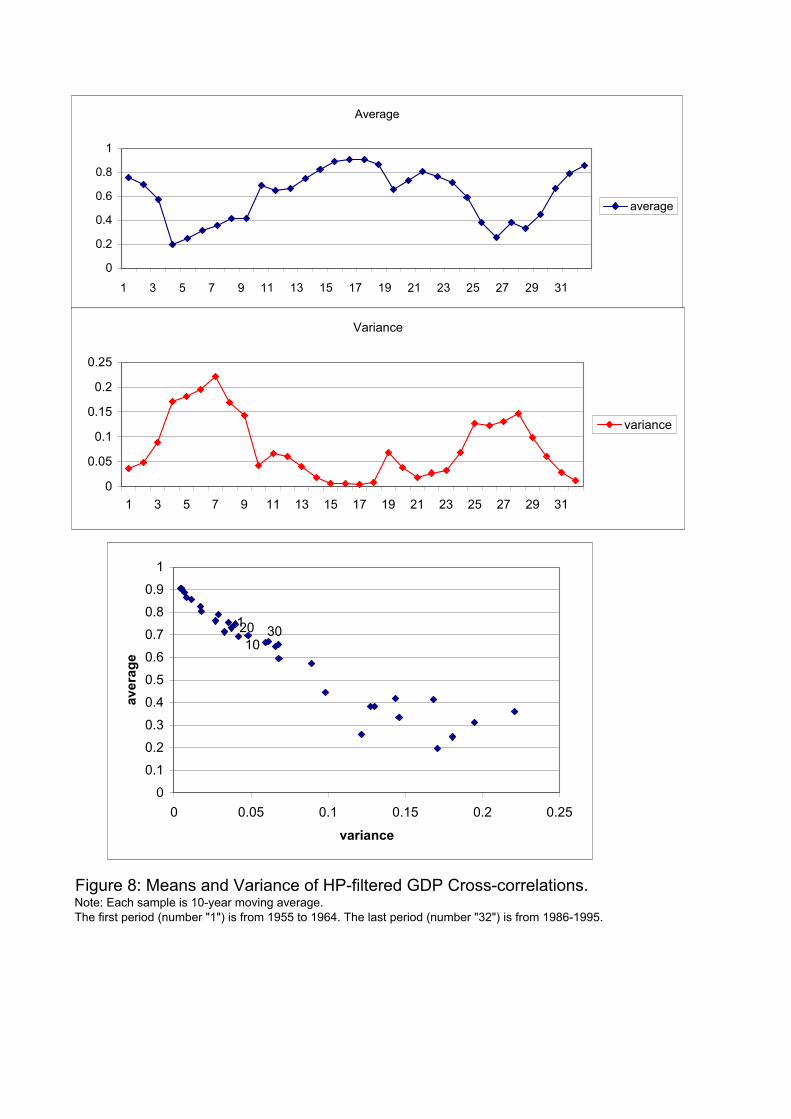
Figure 8: Means and Variance of HP-filtered GDP Cross-correlations.Note: Each sample is 10-year moving average.

The first period (number "1") is from 1955 to 1964. The last period (number "32") is from 1986-1995.

Average

0

0.2

0.4

0.6

0.8

1

1 3 5 7 9 11 13 15 17 19 21 23 25 27 29 31

average

Variance

0

0.05

0.1

0.15

0.2

0.25

1 3 5 7 9 11 13 15 17 19 21 23 25 27 29 31

variance

1

10

20 30

0

0.1

0.2

0.3

0.4

0.5

0.6

0.7

0.8

0.9

1

0 0.05 0.1 0.15 0.2 0.25

variance

av

era

ge

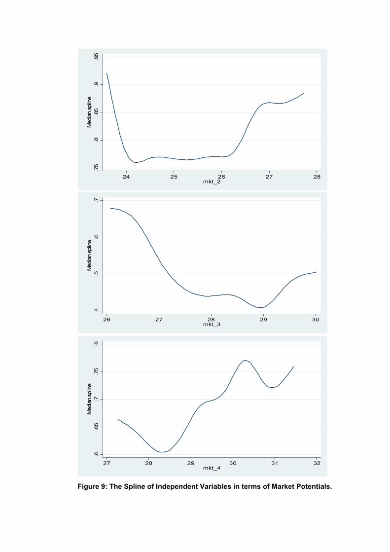
Figure 9: The Spline of Independent Variables in terms of Market Potentials.

.6.6

5.7

.75

.8

Media

n s

plin

e

27 28 29 30 31 32mkt_4

.4.5

.6.7

Media

n s

plin

e

26 27 28 29 30mkt_3

.75

.8.8

5.9

.95

Media

n s

plin

e

24 25 26 27 28mkt_2

Figure10: Consumption Risk Sharing.

-0.2

0

0.2

0.4

0.6

0.8

1

0 0.2 0.4 0.6 0.8 1

Consumption Correlations

Outp

ut C

orr

ela

tions

Fig

ure

A:

Sp

ati

al A

uto

co

rrela

tio

ns.

Mo

ran

's I S

tati

sti

c

-0.2

-0.1

8

-0.1

6

-0.1

4

-0.1

2

-0.1

-0.0

8

-0.0

6

-0.0

4

-0.0

20

19

55

19

60

19

65

19

70

19

75

19

80

19

85

19

90

19

95

Ye

ar

Geary

's C

sta

tisti

c

0.6

0.7

0.8

0.91

1.1

1.2

1955

1959

1963

1967

1971

1975

1979

1983

1987

1991

1995

Year

1955-1

964

1965-1

974

1975-1

984

1985-1

995

HP

corr

ela

tions

0.9

5-1

0.9

-0.9

5

0.8

5-0

.9

0.8

-0.8

5

0.7

5-0

.8

0.7

-0.7

5

0-0

.7

Fig

ure

B: Japanese M

ap a

nd H

P-f

iltere

d G

DP

Cro

ss-c

orr

ela

tions.

Figure C: Employment Cross-correlations in Manufacturing Sectors.

GM

M1

23

45

De

pe

nd

en

t V

ar

Co

eff

icie

nt

z-v

alu

eC

oe

ffic

ien

t

z-v

alu

eC

oe

ffic

ien

t

z

-va

lue

Co

eff

icie

nt

z-v

alu

eC

oe

ffic

ien

t

z

-va

lue

MK

T2

-6.7

19

86

1-7

.27

**-6

.40

68

-6.9

1**

-6.1

73

88

6-6

.11

**

MK

T3

-6.8

06

30

9-5

.97

**-5

.53

61

-4.8

2**

-5.0

06

39

7-3

.77

**

MK

T4

-4.1

79

61

5-0

.87

2.0

34

20

.32

12

.69

67

81

.03

MK

T2_square

0.1

29

75

47

.14

**0

.12

30

6.7

3**

0.1

18

38

5.9

3**

MK

T3_square

0.1

18

25

55

.75

**0

.09

42

4.5

3**

0.0

84

46

33

.50

**

MK

T4_square

0.0

69

84

90

.84

-0.0

39

0-0

.35

-0.2

25

11

3-1

.05

GD

P2

0.0

69

65

.00

**0

.08

79

05

5.5

1**

0.0

74

50

44

.69

**0

.07

71

4.8

6**

0.0

88

12

74

.89

**

GD

P3

0.0

21

41

.48

0.0

11

72

90

.69

0.0

78

80

34

.53

**0

.08

81

5.0

8**

0.0

75

67

34

.15

**

GD

P4

0.1

07

67

.97

**0

.06

27

94

1.7

9*

0.1

28

03

24

.56

**0

.17

11

4.2

7**

0.1

62

96

73

.89

**

gap2

-0.3

08

36

5-3

.14

**-0

.18

80

58

-1.8

3*

gap3

0.1

63

11

61

.08

0.2

82

28

81

.69

*

gap4

0.7

91

27

61

.41

1.4

18

17

11

.60

Openness2

0.6

74

41

.77

*0

.68

29

26

1.6

9*

Openness3

0.8

31

33

.17

**0

.91

68

38

3.2

7**

Openness4

0.9

00

21

.55

1.5

57

97

11

.79

*

AR

EA

0.0

29

95

.24

**0

.04

85

08

8.7

2**

9.9

07

11

51

55

6.7

**0

.70

91

0.0

42

.85

34

42

26

.99

**

Neig

hbour

0.0

11

70

.46

0.0

10

12

30

.39

0.0

10

23

10

.42

0.0

10

60

.43

0.0

09

38

60

.36

Dis

tance

-0.0

29

6-2

.83

**-0

.03

17

14

-2.8

3**

-0.0

04

87

9-0

.36

81

.48

28

6.8

4**

-0.0

39

16

6-1

.49

tim

e2

-1.5

83

8-4

.09

**-2

.01

78

74

-4.6

7**

85

.17

63

7.1

6**

78

.07

22

4.8

7**

78

.26

32

6.0

4**

tim

e3

-0.8

25

7-1

.89

*-0

.56

44

91

-1.1

29

5.1

72

55

.96

**-3

1.5

09

1-0

.34

71

.22

40

83

.87

**

tim

e4

-3.2

65

5-7

.70

**-2

.01

70

26

-2.0

2**

58

.50

61

10

.83

-0.0

16

4-1

.09

-18

4.2

01

7-1

.04

Ha

nse

n's

J

0.0

00

0H

an

se

n's

J

0.0

00

0H

an

se

n's

J

0.0

04

4H

an

se

n's

J

0.0

04

Ha

nse

n's

J

0.0

17

7

Ro

ot

MS

E

=

0

.35

85

Ro

ot

MS

E

=

0

.36

78

Ro

ot

MS

E

=

0

.34

93

Ro

ot

MS

E

=

0

.34

8R

oo

t M

SE

=

0.3

79

1

Tab

le 1

: E

sti

mati

on

Resu

lts 1

(G

DP

, M

ark

et

Po

ten

tial

an

d O

pp

en

ness).

No

tes:

Th

e n

um

be

r o

f sa

mp

le 4

14

0

Co

nsta

nt

term

s a

re o

mitte

d.

Ind

ep

en

de

nt

va

r: H

P-f

ilte

red

GD

P c

orr

ela

tio

ns

* S

ign

ific

an

t a

t th

e 1

0 p

er

ce

nt

leve

l.

** S

ign

ific

an

t a

t th

e 5

pe

r ce

nt

leve

l.

GM

M1

23

4

De

pe

nd

en

t V

ar

Co

eff

icie

nt

z-v

alu

eC

oe

ffic

ien

t

z-v

alu

eC

oe

ffic

ien

t

z-v

alu

eC

oe

ffic

ien

t

z-v

alu

e

MK

T2

-6.1

05

61

-6.0

3**

-9.3

55

6-9

.30

**-8

.34

41

-8.1

9**

-8.8

82

76

-8.1

4**

MK

T3

-4.9

37

81

-4.0

7**

-6.5

86

6-5

.36

**-5

.45

14

-4.4

1**

-5.5

57

41

-4.1

4**

MK

T4

10

.67

21

.13

-4.6

39

8-0

.59

4.0

28

41

0.5

0-1

.83

14

3-0

.19

MK

T2_square

0.1

16

57

5.8

3**

0.1

72

27

8.7

5**

0.1

55

13

7.7

2**

0.1

63

27

7.6

5**

MK

T3_square

0.0

83

02

3.7

7**

0.1

06

35

4.7

7**

0.0

89

99

4.0

0**

0.0

88

78

3.6

9**

MK

T4_square

-0.1

89

46

-1.1

60

.06

22

50

.45

-0.0

73

9-0

.53

0.0

15

98

0.0

9

GD

P2

0.0

76

94

4.2

9**

1.3

15

42

9.6

3**

1.0

19

51

8.0

4**

1.3

09

35

9.2

7**

GD

P3

0.0

90

49

5.0

3**

0.8

96

26

4.4

1**

0.2

94

23

1.5

70

.66

25

42

.63

**

GD

P4

0.2

42

47

3.5

1**

0.9

47

06

1.3

5-0

.70

88

-0.9

50

.52

82

10

.55

Hum

an2

1.5

02

64

9.2

1**

1.1

47

76

7.5

5**

1.4

99

13

8.8

7**

Hum

an3

0.9

50

84

4.0

4**

0.2

81

92

1.3

00

.71

05

72

.47

**

Hum

an4

0.9

58

62

1.2

2-0

.95

72

-1.1

60

.47

06

40

.44

CapLabour2

0.0

59

50

.36

0.0

24

58

0.2

00

.02

77

80

.21

0.0

73

32

0.5

5

CapLabour3

0.0

53

89

0.2

30

.07

04

90

.43

0.1

07

44

0.6

00

.16

28

40

.91

CapLabour4

5.7

59

13

1.8

6*

5.6

15

79

2.6

5**

6.0

45

98

2.4

6**

6.6

60

98

2.6

8**

Cappub2

-0.5

13

2-4

.11

**-0

.29

91

1-1

.97

**

Cappub3

-0.8

53

-6.0

2**

-0.3

50

05

-1.6

5*

Cappub4

-2.3

06

1-6

.34

**-2

.14

49

5-2

.95

**

Infr

a2

-0.2

17

9-1

.95

*-0

.24

18

8-2

.10

**

Infr

a3

-0.4

77

4-3

.59

**-0

.49

44

-3.0

0**

Infr

a4

-0.8

53

7-1

.95

*-0

.10

08

7-0

.15

Openness2

1.1

98

82

.27

**3

.17

28

35

.92

**2

.65

87

64

.88

**3

.15

95

25

.80

**

Openness3

1.1

51

98

3.4

0**

2.2

31

16

4.3

5**

1.0

46

71

2.1

3**

1.7

47

57

2.9

4**

Openness4

1.4

47

08

1.7

8*

1.8

33

94

1.0

7-0

.79

88

-0.4

31

.00

61

60

.48

AR

EA

3.0

88

92

0.2

60

.03

62

0.0

02

2.7

94

42

47

2.7

0**

1.9

98

63

20

4.7

3**

Neig

hbour

0.0

07

30

.20

0.0

06

36

0.1

80

.00

67

10

.19

0.0

06

22

0.1

6

Dis

tance

-0.0

41

38

-1.7

2*

-0.0

13

9-0

.70

-0.0

29

2-1

.39

-0.0

21

99

-0.9

3

tim

e2

77

.90

43

6.0

0**

13

3.0

43

10

.04

**1

15

.89

38

.78

**1

26

.14

58

.73

**

tim

e3

70

.00

56

4.1

4**

10

2.2

51

5.9

0**

80

.17

82

4.6

5**

85

.80

69

4.4

5**

tim

e4

-15

8.7

31

-1.1

58

5.2

57

0.7

5-6

1.1

36

-0.5

34

1.2

00

60

.28

Ha

nse

n's

J

0.0

02

1H

an

se

n's

J

0.0

05

Ha

nse

n's

J

0.1

26

9H

an

se

n's

J

0.0

05

2

Ro

ot

MS

E

=

0

.51

44

Ro

ot

MS

E

=

0

.50

03

Ro

ot

MS

E

=

0

.51

29

Ro

ot

MS

E

=

0

.54

55

No

tes:

Tab

le 2

: E

sti

mati

on

Resu

lts 2

(F

acto

r E

nd

ow

men

ts).

Th

e n

um

be

r o

f sa

mp

le 4

14

0

Co

nsta

nt

term

s a

re o

mitte

d.

* S

ign

ific

an

t a

t th

e 1

0 p

er

ce

nt

leve

l.

Ind

ep

en

de

nt

va

r: H

P-f

ilte

red

GD

P c

orr

ela

tio

ns

** S

ign

ific

an

t a

t th

e 5

pe

r ce

nt

leve

l.

GM

M1

23

45

Dependent V

ar

Coeffic

ient

z-v

alu

eC

oeffic

ient

z-v

alu

eC

oeffic

ient

z-v

alu

eC

oeffic

ient

z-v

alu

eC

oeffic

ient

z-v

alu

e

MK

T2

-8.1

932

-8.2

9**

-9.1

435

-8.6

0**

-9.8

948

-9.1

3**

-9.1

314

-8.4

4**

-9.3

514

-7.7

6**

MK

T3

-5.4

928

-4.4

8**

-5.0

82

-3.8

8**

-5.8

203

-4.5

9**

-5.1

579

-4.0

2**

-5.3

127

-3.6

9**

MK

T4

-12.5

851

-1.5

49.7

3802

0.5

7-0

.3228

-0.0

214.5

888

0.9

49.0

0097

0.4

9

MK

T2

_sq

ua

re0.1

547

8.0

3**

0.1

7099

8.3

2**

0.1

8222

8.7

5**

0.1

704

8.1

1**

0.1

7191

7.4

1**

MK

T3

_sq

ua

re0.0

951

4.3

1**

0.0

8552

3.7

1**

0.0

9378

4.1

9**

0.0

8575

3.7

7**

0.0

8483

3.3

4**

MK

T4

_sq

ua

re0.2

121

1.5

0-0

.1697

-0.5

9-0

.0122

-0.0

5-0

.2539

-0.9

7-0

.1691

-0.5

4

GD

P2

0.0

536

3.2

1**

0.7

4734

6.1

0**

1.1

9894

8.1

0**

0.7

6526

4.7

1**

1.1

9031

7.9

1**

GD

P3

0.1

066

5.8

5**

0.4

5189

1.4

91.2

7214

4.5

6**

0.4

719

1.5

91.0

5529

3.6

3**

GD

P4

0.1

857

4.8

5**

-2.0

277

-0.8

30.2

674

0.1

3-2

.6567

-1.2

0-0

.8875

-0.3

9

Hu

ma

n2

0.8

3604

5.8

9**

1.3

7693

7.8

8**

0.8

6167

4.5

0**

1.3

7073

7.6

5**

Hu

ma

n3

0.4

1356

1.2

21.3

7185

4.3

7**

0.4

596

1.3

71.1

4559

3.4

9**

Hu

ma

n4

-2.5

47

-0.9

30.2

0249

0.0

9-3

.2074

-1.3

0-1

.0982

-0.4

4

Ca

pL

ab

ou

r20.0

1416

0.1

00.0

1179

0.0

80.0

6426

0.4

60.0

7294

0.4

9

Ca

pL

ab

ou

r3-0

.0407

-0.2

0-0

.0514

-0.2

70.0

6666

0.3

50.0

6274

0.3

1

Ca

pL

ab

ou

r45.8

485

1.7

1*

5.5

0119

1.7

2*

7.4

6542

2.2

7**

7.2

8699

2.0

3**

Ca

pp

ub

2-0

.4481

-3.9

0**

-0.2

359

-1.6

5*

Ca

pp

ub

3-0

.7753

-6.3

4**

-0.4

032

-1.9

8**

Ca

pp

ub

4-2

.3448

-5.2

4**

-2.8

079

-4.3

9**

Infr

a2

-0.0

469

-0.3

9-0

.2319

-2.0

5**

Infr

a3

-0.2

184

-1.6

4*

-0.3

65

-2.3

6**

Infr

a4

-0.5

142

-1.3

30.2

8597

0.6

0

Op

en

ne

ss2

1.4

423

3.3

0**

2.3

5711

4.6

1**

3.2

6581

5.9

7**

2.5

556

4.4

8**

3.2

3176

5.6

6**

Op

en

ne

ss3

0.5

686

1.9

4*

1.5

1744

2.0

7**

2.5

3607

3.6

8**

1.4

8179

2.0

6**

2.2

4347

3.1

0**

Op

en

ne

ss4

0.7

612

1.3

0-0

.779

-0.2

01.3

8284

0.3

9-1

.9138

-0.5

2-0

.43

-0.1

1

CV

21.2

822

2.9

4**

1.1

7808

2.1

3**

0.6

5704

1.2

11.2

535

2.1

4**

0.6

4187

1.2

0

CV

3-2

.3634

-4.1

0**

-1.5

403

-2.0

3**

-2.7

533

-3.9

2**

-1.1

793

-1.6

5*

-2.1

422

-3.2

7**

CV

40.6

198

0.5

47.2

29

1.8

9*

3.4

2152

1.0

38.7

9369

2.4

1**

4.9

7852

1.4

7

CL

22.5

866

0.8

3-2

.4896

-0.6

90.3

6097

0.1

1-2

.9362

-0.8

10.3

4419

0.1

0

CL

312.0

914

4.2

2**

7.1

0655

1.4

711.1

432

2.5

9**

5.4

6303

1.2

69.4

764

2.2

5**

CL

411.8

518

2.7

0**

-29.9

94

-1.0

1-1

7.8

77

-0.6

6-4

0.9

17

-1.5

1-3

4.5

94

-1.1

9

AR

EA

0.0

045

0.0

00.0

2293

0.0

01.4

0269

0.0

60.0

2426

0.0

00.3

2325

0.0

1

Ne

igh

bo

ur

0.0

100

0.4

10.0

0649

0.1

90.0

0649

0.1

90.0

0596

0.1

50.0

058

0.1

5

Dis

tan

ce

0.0

072

0.4

2-0

.0353

-1.0

3-0

.02

-0.6

6-0

.0458

-1.4

0-0

.0381

-1.0

2

tim

e2

106.4

864

8.3

0**

124.8

75

8.8

6**

139.7

04

9.6

4**

124.9

65

8.7

8**

131.8

84

8.1

6**

tim

e3

76.5

540

4.4

5**

73.7

125

3.8

6**

92.4

228

5.0

2**

75.8

882

4.0

8**

83.8

577

3.9

7**

tim

e4

180.3

838

1.5

2-1

53.3

-0.6

021.0

529

0.1

0-2

23.3

3-0

.96

-118.2

2-0

.43

**

Hansen's

J 0.0

083

Hansen's

J 0.0

102

Hansen's

J 0.0

287

Hansen's

J 0.0

224

Hansen's

J 0.0

128

Root M

SE

=

0.3

471

Root M

SE

=

0.5

044

Root M

SE

=

0.4

885

Root M

SE

=

0.5

806

Root M

SE

=

0.5

72

Ta

ble

3:

Es

tim

ati

on

Re

su

lts

3 (

Ind

us

tria

l S

tru

ctu

re a

nd

Fa

cto

r E

nd

ow

me

nts

).N

ote

The n

um

ber

of sam

ple

4140

Consta

nt te

rms a

re o

mitte

d.

Independent var:

HP

-filt

ere

d G

DP

corr

ela

tions

* S

ignific

ant at th

e 1

0 p

er

cent le

vel.

** S

ignific

ant at th

e 5

per

cent le

vel.

Pre

fectu

re1

23

45

67

89

10

11

12

13

14

15

16

17

18

19

20

21

22

23

24

25

26

27

1 20

.20

14

30

.30

05

0.6

51

9

40

.37

09

0.6

15

0.8

14

2

50

.07

13

0.4

48

30

.65

31

0.8

14

4

60

.53

0.5

63

30

.78

85

0.9

11

60

.80

65

70

.46

77

0.5

11

0.8

90

20

.87

70

.73

68

0.9

14

6

80

.30

32

0.3

53

80

.39

14

0.7

05

10

.59

91

0.5

85

0.4

15

3

90

.21

58

0.3

94

0.6

99

20

.91

93

0.7

45

10

.82

71

0.7

97

50

.73

33

10

0.4

10

.35

60

.34

20

.72

82

0.4

81

50

.63

64

0.5

51

30

.80

84

0.8

04

7

11

0.7

29

70

.67

44

0.7

96

70

.83

60

.51

43

0.8

22

80

.82

81

0.5

04

10

.62

31

0.5

58

7

12

0.6

91

90

.46

54

0.5

87

70

.88

22

0.5

72

10

.86

08

0.7

77

20

.66

44

0.7

96

0.8

15

10

.87

27

13

0.3

38

90

.54

82

0.3

89

50

.63

44

0.6

30

90

.77

67

0.4

70

10

.56

53

0.5

75

90

.51

02

0.4

94

70

.62

99

14

0.1

59

20

.44

85

0.6

80

10

.77

02

0.8

53

0.8

36

60

.69

24

0.4

30

20

.67

46

0.2

77

10

.55

28

0.5

77

0.7

73

6

15

0.5

13

40

.85

93

0.7

49

90

.66

81

0.5

83

90

.77

61

0.7

36

30

.36

79

0.4

39

80

.38

95

0.8

05

10

.59

55

0.6

21

0.5

60

6

16

0.4

50

40

.14

67

0.5

64

50

.76

79

0.7

44

80

.79

66

0.6

61

20

.79

04

0.7

81

90

.60

04

0.5

88

70

.72

89

0.6

22

90

.73

59

0.3

86

7

17

-0.1

55

4-0

.23

75

0.2

31

70

.14

17

-0.0

35

1-0

.08

53

0.2

59

8-0

.00

33

0.2

92

20

.19

69

0.0

39

30

.04

6-0

.60

62

-0.2

72

3-0

.25

69

-0.0

12

9

18

0.4

68

30

.69

33

0.6

90

10

.90

08

0.7

48

20

.85

73

0.8

23

60

.71

17

0.7

99

0.8

29

70

.81

88

0.8

57

0.6

11

50

.55

81

0.7

89

90

.62

85

0.0

81

7

19

0.3

66

70

.53

07

0.7

91

50

.91

43

0.7

19

10

.89

11

0.7

92

90

.76

66

0.9

26

70

.70

56

0.7

33

20

.80

06

0.7

21

0.7

64

50

.60

52

0.8

41

60

.04

38

0.7

81

6

20

0.5

06

10

.44

94

0.7

96

90

.92

49

0.7

43

0.9

23

70

.85

38

0.7

65

50

.90

70

.71

15

0.8

00

20

.85

89

0.6

62

70

.75

16

0.6

19

20

.90

86

0.0

93

40

.81

18

0.9

71

1

21

0.2

81

50

.28

78

0.8

07

0.8

20

70

.74

39

0.7

01

70

.78

08

0.6

20

40

.75

52

0.4

42

70

.68

65

0.6

29

70

.26

05

0.6

51

60

.43

20

.80

70

.38

20

.64

15

0.7

57

30

.83

53

22

0.6

61

60

.52

60

.68

57

0.8

32

0.5

66

60

.84

44

0.7

16

0.8

22

10

.77

83

0.7

50

80

.83

31

0.8

65

80

.69

10

.58

99

0.6

68

40

.83

08

-0.0

63

20

.80

32

0.9

13

40

.93

68

0.6

83

9

23

0.4

42

80

.42

99

0.8

27

60

.70

86

0.7

26

0.8

60

30

.80

23

0.4

08

70

.59

85

0.2

35

80

.69

05

0.5

68

40

.63

36

0.8

53

50

.70

75

0.7

70

9-0

.16

24

0.5

67

80

.77

61

0.8

20

40

.73

02

0.7

18

7

24

0.3

42

40

.50

03

0.8

54

60

.88

99

0.7

05

60

.81

82

0.8

09

70

.77

84

0.8

95

10

.66

89

0.7

39

0.7

28

80

.52

11

0.6

55

50

.59

27

0.8

24

0.2

38

90

.77

74

0.9

54

10

.95

38

0.8

67

50

.88

77

0.7

59

2

25

0.2

00

70

.54

84

0.9

11

60

.78

78

0.7

42

0.7

20

10

.83

35

0.2

96

10

.60

25

0.1

95

20

.73

66

0.5

33

50

.29

96

0.7

44

90

.64

12

0.5

44

80

.21

95

0.6

15

60

.64

40

.69

0.8

56

20

.51

50

.77

91

0.7

13

4

26

0.3

52

80

.75

48

0.8

47

80

.92

43

0.7

80

.92

12

0.8

13

20

.63

10

.80

76

0.5

62

30

.81

16

0.7

72

30

.79

17

0.8

57

90

.79

43

0.7

12

2-0

.14

65

0.8

17

70

.92

42

0.8

88

80

.69

76

0.8

38

50

.82

20

.85

65

0.7

66

7

27

0.4

96

30

.41

96

0.5

43

90

.80

32

0.4

23

30

.74

87

0.6

05

0.7

14

80

.83

37

0.7

77

0.7

03

0.8

70

80

.67

37

0.5

56

20

.41

53

0.7

11

50

.01

28

0.6

74

10

.88

60

.85

08

0.5

37

30

.87

73

0.5

12

60

.77

77

0.3

79

0.7

72

3

28

0.4

09

50

.24

74

0.3

05

60

.73

72

0.7

60

60

.72

57

0.5

21

10

.84

33

0.7

09

90

.77

19

0.5

24

50

.77

29

0.6

96

40

.61

17

0.4

02

20

.84

37

-0.1

58

50

.75

33

0.6

86

60

.74

79

0.5

82

70

.73

05

0.4

89

0.6

20

90

.34

86

0.6

28

0.6

41

2

29

0.6

54

30

.27

17

0.1

30

70

.40

91

0.1

72

90

.54

62

0.4

17

60

.46

39

0.4

61

10

.79

08

0.4

67

20

.68

08

0.5

41

50

.09

42

0.4

53

70

.36

05

-0.1

17

0.6

35

10

.45

60

.48

26

0.0

28

60

.61

71

0.1

91

70

.34

89

-0.1

00

30

.36

31

0.5

99

6

30

0.4

78

0.5

45

80

.90

39

0.8

47

80

.71

67

0.8

54

70

.93

35

0.5

92

70

.77

80

.59

86

0.8

20

90

.71

94

0.4

23

70

.58

88

0.7

64

90

.71

08

0.2

76

80

.84

71

0.8

21

90

.88

17

0.8

35

20

.80

74

0.7

96

30

.90

54

0.7

88

50

.79

89

0.5

86

9

31

0.2

65

0.4

68

30

.85

08

0.8

80

40

.82

93

0.8

28

30

.91

25

0.6

31

80

.86

57

0.6

44

50

.69

70

.68

36

0.4

04

20

.63

32

0.6

36

80

.73

13

0.3

73

30

.84

82

0.8

20

80

.86

48

0.8

70

60

.71

95

0.7

21

70

.90

06

0.7

91

50

.77

50

.55

97

32

0.1

07

80

.04

91

0.4

96

10

.65

25

0.7

35

60

.58

50

.62

0.7

31

70

.77

80

.65

81

0.3

41

40

.49

58

0.2

64

20

.43

51

0.2

45

90

.77

91

0.4

22

40

.63

49

0.6

63

70

.72

52

0.7

69

30

.57

90

.49

12

0.7

63

40

.46

10

.47

39

0.4

28

8

33

0.2

82

10

.43

71

0.7

69

30

.93

91

0.9

35

90

.91

24

0.8

62

80

.69

24

0.8

94

20

.62

79

0.6

95

80

.77

21

0.6

40

70

.85

80

.59

35

0.8

72

30

.10

02

0.8

20

60

.88

13

0.9

17

70

.86

71

0.7

61

80

.79

98

0.8

67

70

.79

24

0.8

68

60

.66

95

34

0.4

00

90

.38

11

0.5

36

90

.49

41

0.7

03

10

.76

49

0.6

41

30

.35

46

0.4

17

70

.27

40

.46

06

0.4

18

40

.70

07

0.6

81

20

.73

65

0.6

13

5-0

.38

12

0.5

68

90

.56

25

0.6

11

20

.40

08

0.5

62

90

.82

44

0.5

14

0.4

60

60

.63

30

.27

22

35

0.0

00

1-0

.15

40

.57

14

0.4

83

10

.34

41

0.3

79

10

.59

64

0.2

22

70

.65

29

0.2

89

90

.27

13

0.3

24

1-0

.11

98

0.3

02

1-0

.03

75

0.4

87

30

.76

81

0.2

50

40

.51

55

0.5

51

90

.70

19

0.3

15

60

.40

02

0.6

20

50

.52

36

0.3

0.3

86

3

36

-0.0

43

90

.08

72

0.6

54

90

.75

09

0.7

58

90

.61

57

0.7

19

0.4

83

20

.82

70

.45

09

0.4

05

0.5

09

60

.20

75

0.6

37

90

.17

71

0.7

03

40

.52

92

0.5

31

10

.68

27

0.7

17

40

.86

84

0.4

52

50

.55

70

.74

37

0.7

26

70

.57

0.4

72

4

37

0.3

77

70

.56

71

0.5

99

70

.87

27

0.8

94

50

.89

19

0.7

92

10

.66

53

0.7

71

80

.72

72

0.6

98

50

.80

43

0.7

26

20

.73

08

0.7

24

50

.71

2-0

.08

89

0.9

29

50

.74

32

0.7

86

20

.62

80

.71

29

0.6

41

70

.69

0.6

20

30

.80

76

0.5

86

5

38

0.2

23

90

.32

17

0.7

55

30

.89

77

0.9

09

20

.82

79

0.8

41

40

.65

21

0.8

64

10

.57

02

0.6

45

80

.70

83

0.4

70

10

.78

80

.48

34

0.8

53

0.2

60

70

.75

50

.81

18

0.8

71

80

.93

0.6

82

30

.74

72

0.8

46

90

.81

96

0.7

73

20

.58

36

39

0.3

52

50

.39

06

0.6

66

10

.90

46

0.9

16

80

.88

44

0.7

84

70

.79

96

0.8

62

40

.69

46

0.6

74

80

.79

04

0.6

71

50

.80

07

0.5

67

80

.92

18

0.0

23

90

.83

16

0.8

62

50

.91

40

.83

59

0.8

06

90

.75

39

0.8

49

20

.68

55

0.8

24

70

.67

79

40

0.1

53

70

.22

64

0.2

76

10

.55

95

0.7

60

20

.67

94

0.4

17

70

.71

35

0.6

28

60

.57

23

0.2

50

90

.48

39

0.8

24

30

.68

16

0.3

99

40

.76

67

-0.3

70

20

.57

18

0.6

71

80

.65

66

0.3

85

70

.61

11

0.5

76

10

.56

28

0.2

18

10

.61

06

0.5

01

2

41

0.4

53

1-0

.00

69

0.3

42

90

.27

35

0.2

03

30

.52

61

0.5

69

30

.12

95

0.4

27

50

.41

79

0.2

85

0.3

78

90

.29

24

0.1

74

20

.35

55

0.3

65

60

.16

11

0.3

78

50

.41

94

0.4

66

80

.16

75

0.4

23

30

.44

62

0.3

92

70

.08

84

0.2

67

50

.33

91

42

0.2

86

60

.38

80

.10

71

0.2

45

90

.54

92

0.4

36

80

.22

47

0.1

96

50

.00

36

0.0

63

10

.28

78

0.2

49

0.6

04

30

.49

90

.58

35

0.2

87

6-0

.70

03

0.3

92

70

.13

01

0.1

92

0.0

83

10

.22

73

0.4

25

90

.04

08

0.2

47

90

.37

09

-0.0

33

7

43

0.2

69

60

.14

17

0.1

82

40

.67

71

0.5

18

40

.55

63

0.4

81

90

.67

63

0.7

63

50

.91

28

0.4

15

30

.76

91

0.4

22

40

.30

96

0.1

68

60

.56

62

0.2

49

20

.71

54

0.5

63

40

.59

42

0.4

18

90

.54

54

0.1

20

30

.49

85

0.1

80

30

.43

11

0.6

66

6

44

0.3

38

60

.25

33

-0.2

10

2-0

.16

63

-0.3

17

9-0

.09

34

-0.0

98

0.0

69

6-0

.17

37

0.3

47

20

.07

48

0.0

63

7-0

.01

41

-0.5

35

70

.27

84

-0.3

17

3-0

.07

70

.24

04

-0.1

64

3-0

.16

12

-0.4

26

60

.08

8-0

.33

37

-0.1

45

6-0

.43

98

-0.1

63

2-0

.04

45

0.2

27

10

.42

82

0.9

11

60

.79

66

0.7

83

50

.83

86

0.9

42

0.3

65

20

.77

15

0.3

89

70

.65

05

0.5

70

50

.41

23

0.7

38

50

.64

40

.65

60

.28

89

0.6

85

70

.77

36

0.8

06

60

.80

59

0.6

07

0.8

47

0.8

17

30

.85

67

0.7

74

70

.47

52

46

0.3

94

80

.63

02

0.4

03

60

.76

23

0.4

37

50

.67

50

.54

29

0.4

90

50

.66

04

0.7

21

80

.69

45

0.8

45

40

.66

07

0.4

98

20

.52

05

0.3

85

5-0

.11

42

0.7

46

60

.63

34

0.5

94

20

.30

56

0.6

24

90

.28

04

0.4

79

50

.37

02

0.7

08

10

.79

13

47

-0.1

33

90

.09

83

0.6

98

90

.53

27

0.5

05

0.4

38

10

.61

20

.38

28

0.6

91

40

.31

08

0.2

64

50

.23

59

0.0

30

50

.38

85

0.1

76

70

.51

86

0.6

24

10

.36

47

0.6

25

20

.61

03

0.7

31

40

.40

34

0.5

16

60

.75

65

0.5

81

90

.45

03

0.3

49

4

To

atl

0.5

00

50

.55

34

0.7

21

0.9

04

80

.81

42

0.9

72

50

.81

55

0.7

22

40

.83

71

0.6

78

0.7

76

10

.85

28

0.8

53

10

.84

93

0.7

26

60

.86

57

-0.1

86

70

.83

98

0.9

29

80

.94

37

0.6

94

40

.89

92

0.8

39

60

.84

43

0.6

43

70

.93

43

0.8

03

2

Tab

le A

: H

p-f

ilte

red

GD

P C

ross-c

orr

ela

tio

ns in

Jap

an

(1955-1

964).

28

29

30

31

32

33

34

35

36

37

38

39

40

41

42

43

44

45

46

47

0.5

41

4

0.5

47

30

.41

51

0.6

18

10

.33

63

0.9

54

1

0.7

01

10

.29

63

0.7

29

10

.84

95

0.7

97

70

.31

04

0.8

39

20

.90

96

0.7

85

0.5

36

90

.42

07

0.6

56

90

.59

62

0.4

70

70

.64

77

0.1

42

-0.0

28

60

.56

56

0.6

51

30

.65

33

0.5

32

10

.06

58

0.5

25

6-0

.00

72

0.6

74

50

.83

02

0.8

17

70

.84

19

0.2

89

70

.84

37

0.8

59

40

.54

70

.75

70

.80

84

0.6

58

80

.89

35

0.7

01

80

.19

60

.58

76

0.7

45

10

.18

78

0.8

27

0.9

18

90

.83

38

0.9

77

30

.54

90

.63

88

0.9

16

40

.82

25

0.8

98

10

.38

92

0.8

05

0.8

67

80

.81

79

0.9

76

30

.65

94

0.4

33

0.7

70

40

.90

92

0.9

47

2

0.8

28

0.4

72

70

.46

13

0.5

37

60

.65

24

0.7

11

70

.75

04

0.0

79

80

.42

27

0.7

43

50

.61

02

0.7

87

3

0.2

09

90

.68

23

0.5

40

30

.46

95

0.4

31

10

.33

05

0.5

99

90

.41

79

0.2

37

50

.34

52

0.2

75

10

.31

21

0.3

82

2

0.5

16

20

.20

81

0.2

00

50

.16

77

0.0

65

40

.35

87

0.6

97

9-0

.51

04

-0.0

80

40

.59

98

0.2

58

10

.42

52

0.5

50

5-0

.00

88

0.8

00

20

.64

41

0.4

27

60

.55

68

0.6

35

70

.62

62

0.1

48

50

.32

42

0.5

50

90

.71

52

0.6

04

70

.67

97

0.5

31

70

.27

87

0.0

81

2

-0.0

36

70

.64

89

0.0

26

4-0

.09

68

-0.1

23

7-0

.31

55

0.0

39

3-0

.44

22

-0.5

43

90

.03

71

-0.3

95

4-0

.22

55

-0.0

64

10

.31

60

.07

83

0.1

20

9

0.4

19

0.2

02

20

.90

39

0.9

21

30

.68

25

0.8

58

20

.67

47

0.6

89

20

.79

95

0.6

96

0.8

56

80

.75

80

.45

76

0.5

46

20

.16

64

0.3

21

1-0

.27

16

0.5

94

80

.58

80

.41

54

0.4

24

50

.16

29

0.5

63

80

.17

55

0.0

40

90

.29

08

0.6

93

20

.45

53

0.5

51

50

.35

10

.09

75

0.2

32

50

.71

74

0.1

15

80

.32

26

0.1

81

4-0

.04

37

0.6

89

0.7

72

20

.75

69

0.6

07

90

.27

40

.88

78

0.8

20

10

.29

84

0.6

79

40

.52

08

0.2

77

10

.41

36

-0.3

52

30

.22

43

-0.3

34

70

.78

13

-0.0

20

7

0.8

12

10

.54

36

0.8

02

20

.78

49

0.6

10

90

.91

40

.74

91

0.3

06

70

.58

59

0.8

85

40

.81

75

0.9

20

60

.78

22

0.4

36

80

.46

0.5

80

8-0

.10

84

0.7

51

50

.67

72

0.4

06

2

Pre

fectu

re1

23

45

67

89

10

11

12

13

14

15

16

17

18

19

20

21

22

23

24

25

26

27

1 20

.84

98

30

.96

64

0.8

01

6

40

.85

21

0.7

35

10

.89

05

50

.94

03

0.8

80

40

.85

97

0.8

03

1

60

.91

63

0.8

44

40

.87

74

0.8

38

30

.95

23

70

.92

94

0.8

25

40

.92

40

.72

51

0.8

98

60

.89

57

80

.60

40

.58

93

0.6

00

10

.80

74

0.6

51

40

.56

61

0.4

18

7

90

.67

07

0.2

90

50

.74

56

0.7

13

90

.52

05

0.6

29

30

.58

84

0.3

86

1

10

0.6

93

80

.60

13

0.7

42

0.8

04

40

.73

35

0.7

17

20

.67

04

0.8

15

0.6

51

8

11

0.6

86

80

.29

70

.75

22

0.6

40

60

.60

27

0.6

28

0.7

11

30

.43

96

0.8

08

20

.71

33

12

0.7

25

30

.49

75

0.8

08

50

.77

76

0.6

79

90

.78

30

.73

0.5

68

90

.84

69

0.8

58

50

.86

57

13

0.7

73

70

.56

22

0.8

69

20

.82

76

0.7

22

60

.78

39

0.8

14

50

.60

.79

97

0.8

84

70

.89

59

0.9

51

8

14

0.5

56

20

.31

53

0.6

22

80

.69

24

0.5

75

60

.57

44

0.5

42

60

.69

29

0.7

36

40

.93

41

0.8

24

0.8

57

0.8

73

3

15

0.7

33

60

.91

50

.70

17

0.7

63

40

.84

20

.78

29

0.7

07

50

.77

99

0.2

56

70

.78

13

0.3

12

10

.54

43

0.6

16

30

.52

59

16

0.7

35

40

.64

20

.79

11

0.8

71

10

.74

52

0.7

30

10

.69

32

0.8

21

30

.68

36

0.9

79

30

.68

88

0.8

23

20

.88

59

0.9

02

10

.79

83

17

0.8

65

20

.72

98

0.8

83

80

.90

98

0.8

76

10

.90

52

0.8

14

60

.75

57

0.7

67

0.9

32

80

.75

70

.91

44

0.9

16

60

.84

46

0.7

93

50

.93

48

18

0.9

30

60

.81

21

0.9

58

80

.88

66

0.8

82

60

.89

78

0.9

43

40

.57

46

0.6

66

40

.74

45

0.7

24

70

.76

17

0.8

75

40

.62

95

0.7

52

30

.80

81

0.8

76

19

0.6

57

30

.43

30

.77

47

0.5

82

80

.50

77

0.5

02

10

.76

48

0.2

94

60

.65

81

0.6

27

30

.77

35

0.6

55

40

.81

62

0.6

38

60

.39

19

0.6

85

10

.62

49

0.7

89

9

20

0.8

13

50

.79

24

0.8

61

40

.85

71

0.8

08

20

.79

74

0.7

94

60

.77

39

0.6

29

30

.94

61

0.6

35

10

.82

23

0.8

71

40

.79

31

0.8

73

0.9

58

60

.93

69

0.8

49

0.6

92

2

21

0.7

15

20

.44

85

0.7

76

20

.80

76

0.6

99

90

.79

38

0.7

05

60

.57

21

0.8

81

60

.85

64

0.8

68

10

.95

83

0.9

39

70

.89

63

0.5

27

80

.84

87

0.9

22

60

.78

24

0.6

49

20

.78

64

22

0.6

92

30

.54

51

0.7

82

70

.83

09

0.6

74

70

.72

60

.69

49

0.6

76

50

.79

24

0.9

51

20

.75

59

0.9

03

20

.93

76

0.9

21

80

.67

80

.96

50

.92

89

0.7

97

10

.73

43

0.9

19

70

.92

56

23

0.7

09

90

.45

92

0.7

90

40

.72

70

.67

12

0.6

66

30

.74

50

.63

48

0.7

33

10

.89

76

0.9

31

10

.90

35

0.9

57

40

.92

39

0.5

59

20

.86

91

0.8

60

.77

81

0.8

06

70

.83

40

.88

11

0.8

91

1

24

0.6

94

0.6

67

40

.73

60

.87

67

0.7

39

70

.73

51

0.6

17

70

.89

37

0.5

99

40

.96

89

0.5

91

70

.80

06

0.8

24

40

.85

54

0.8

48

0.9

72

40

.92

66

0.7

42

40

.51

91

0.9

42

10

.80

70

.91

72

0.7

98

4

25

0.8

12

50

.48

32

0.8

76

60

.78

55

0.7

01

20

.77

24

0.7

96

20

.46

20

.94

85

0.7

68

20

.90

33

0.9

17

40

.92

46

0.8

02

70

.44

89

0.7

89

80

.87

44

0.8

35

90

.79

89

0.7

70

80

.93

46

0.8

71

10

.87

05

0.6

95

1

26

0.8

07

20

.63

74

0.8

52

70

.88

17

0.8

22

50

.83

65

0.8

12

70

.72

27

0.7

26

30

.92

59

0.8

35

70

.88

82

0.9

60

.89

05

0.7

37

80

.93

78

0.9

53

60

.90

.73

56

0.8

95

80

.92

74

0.9

36

30

.92

57

0.8

94

70

.86

9

27

0.7

91

90

.60

13

0.8

50

.80

04

0.7

70

60

.74

53

0.8

10

20

.70

24

0.7

20

50

.94

32

0.8

67

30

.88

27

0.9

55

90

.91

34

0.6

96

10

.93

71

0.9

17

90

.85

23

0.8

17

10

.91

80

.87

66

0.9

29

70

.97

72

0.8

69

60

.87

26

0.9

60

2

28

0.4

78

90

.31

58

0.6

12

70

.67

81

0.4

27

0.4

62

30

.47

12

0.6

48

70

.72

70

.90

45

0.6

98

10

.82

22

0.8

43

0.9

24

50

.51

01

0.8

99

20

.78

16

0.5

85

90

.69

0.8

26

30

.81

22

0.9

36

70

.85

82

0.8

49

60

.75

98

0.8

03

20

.86

04

29

0.8

64

10

.68

08

0.8

27

80

.62

83

0.8

66

70

.77

59

0.9

03

30

.52

96

0.5

45

70

.74

10

.80

29

0.7

19

0.7

88

30

.67

75

0.6

49

20

.71

18

0.7

92

50

.81

60

.72

03

0.7

68

40

.68

90

.67

14

0.8

42

0.6

37

0.7

59

20

.81

0.8

73

1

30

0.9

51

10

.84

70

.97

31

0.9

18

30

.88

14

0.9

12

0.9

04

60

.61

39

0.7

35

40

.76

45

0.6

56

40

.78

30

.84

27

0.6

19

40

.77

38

0.8

30

20

.90

98

0.9

63

50

.72

12

0.8

90

10

.78

62

0.8

19

90

.72

84

0.7

85

10

.85

30

.85

96

0.8

22

6

31

0.6

87

40

.75

02

0.7

44

80

.68

56

0.7

14

70

.69

32

0.7

97

60

.53

42

0.4

50

30

.81

61

0.5

14

0.6

44

60

.78

36

0.6

64

10

.82

31

0.8

55

10

.77

99

0.8

27

80

.77

15

0.8

99

20

.64

87

0.8

33

70

.72

79

0.7

84

40

.64

86

0.8

15

30

.83

16

32

0.7

80

70

.78

28

0.7

74

40

.79

39

0.8

21

50

.82

45

0.7

81

10

.57

42

0.6

00

10

.79

20

.47

54

0.6

54

10

.73

26

0.6

48

60

.82

35

0.8

56

80

.85

76

0.8

46

10

.61

74

0.8

69

60

.73

05

0.8

36

10

.62

61

0.8

07

70

.71

81

0.8

18

70

.76

36

33

0.6

87

20

.50

23

0.7

65

20

.71

63

0.6

68

70

.65

06

0.7

14

90

.69

52

0.6

73

60

.93

87

0.8

60

90

.89

23

0.9

31

30

.92

62

0.6

31

0.8

97

0.8

67

70

.73

96

0.7

54

90

.88

04

0.8

44

80

.89

89

0.9

84

40

.84

95

0.8

15

90

.90

62

0.9

74

9

34

0.7

63

40

.46

42

0.8

38

20

.70

37

0.6

59

70

.77

47

0.7

86

30

.37

66

0.8

79

50

.70

10

.89

87

0.9

52

70

.90

82

0.7

23

60

.39

75

0.6

78

50

.82

88

0.7

72

40

.70

73

0.7

07

70

.90

35

0.7

88

50

.84

64

0.6

19

0.9

47

0.8

05

60

.81

03

35

0.7

80

20

.74

41

0.8

19

40

.89

79

0.8

13

90

.79

42

0.7

45

60

.84

61

0.6

04

60

.96

31

0.6

49

30

.80

13

0.8

74

30

.84

08

0.8

81

10

.98

38

0.9

43

50

.85

14

0.6

48

30

.97

0.8

16

20

.92

84

0.8

41

10

.97

68

0.7

45

80

.94

35

0.9

21

6

36

0.6

87

90

.51

04

0.7

45

40

.91

33

0.6

96

20

.74

91

0.5

90

80

.82

71

0.7

24

90

.87

97

0.7

46

90

.86

57

0.8

73

0.8

63

0.6

57

30

.88

73

0.9

08

60

.75

45

0.5

09

20

.80

57

0.9

03

20

.87

89

0.8

26

90

.90

98

0.7

80

80

.91

96

0.8

39

5

37

0.8

85

50

.87

44

0.8

50

90

.84

98

0.9

43

0.9

43

80

.83

03

0.7

54

10

.54

49

0.8

28

0.5

93

90

.79

21

0.7

79

60

.64

75

0.8

88

70

.81

12

0.9

32

10

.83

64

0.4

48

40

.88

58

0.7

55

50

.75

58

0.7

18

10

.85

46

0.7

00

80

.84

42

0.7

98

1

38

0.4

20

30

.40

29

0.4

94

80

.68

68

0.4

89

70

.48

44

0.3

83

60

.78

50

.52

06

0.9

23

40

.49

18

0.6

88

80

.71

89

0.8

81

40

.68

41

0.9

18

50

.77

60

.53

08

0.4

65

40

.82

48

0.7

27

60

.88

82

0.7

28

30

.92

67

0.5

73

60

.78

41

0.7

81

4

39

0.6

34

80

.72

34

0.6

23

0.6

93

0.6

70

90

.66

19

0.5

55

90

.62

40

.50

73

0.7

53

50

.24

54

0.5

47

60

.54

99

0.5

64

60

.79

96

0.7

99

20

.76

38

0.6

18

60

.39

63

0.8

35

30

.57

47

0.7

50

80

.46

60

.80

26

0.5

52

90

.63

09

0.6

20

4

40

0.9

24

0.8

42

90

.94

94

0.8

93

60

.87

37

0.8

54

30

.88

63

0.7

00

90

.68

85

0.8

57

50

.66

55

0.7

80

50

.85

83

0.7

07

90

.83

22

0.9

07

0.9

23

90

.93

70

.76

24

0.9

58

60

.77

14

0.8

67

50

.79

76

0.8

56

80

.82

92

0.8

86

50

.89

57

41

0.7

36

50

.68

90

.78

15

0.7

99

70

.77

33

0.8

58

70

.82

22

0.4

55

0.5

99

70

.71

53

0.6

20

40

.73

78

0.8

37

10

.63

19

0.7

08

70

.77

01

0.8

27

60

.90

56

0.6

66

40

.76

62

0.8

10

70

.81

10

.68

96

0.7

21

60

.75

24

0.8

78

10

.75

93

42

0.5

56

80

.67

01

0.5

91

70

.82

63

0.6

30

10

.63

60

.48

44

0.7

86

90

.39

72

0.7

76

10

.28

36

0.5

28

20

.61

82

0.6

15

50

.84

58

0.8

49

70

.75

54

0.6

82

30

.39

16

0.8

03

20

.60

63

0.7

72

60

.51

59

0.8

82

50

.47

67

0.7

45

90

.64

39

43

0.8

83

30

.69

49

0.8

44

60

.86

03

0.8

72

50

.93

48

0.8

02

30

.51

69

0.7

14

80

.59

90

.65

15

0.7

15

90

.73

18

0.5

31

90

.60

94

0.6

53

60

.83

42

0.8

72

50

.48

24

0.6

56

20

.79

26

0.6

61

70

.59

82

0.6

37

0.7

93

20

.79

56

0.6

62

4

44

0.7

30

30

.54

97

0.8

36

30

.71

76

0.6

47

90

.66

69

0.8

13

50

.48

88

0.7

48

40

.84

48

0.8

18

90

.84

09

0.9

37

70

.82

12

0.5

85

80

.86

76

0.8

28

20

.84

46

0.9

34

10

.87

24

0.8

26

50

.91

49

0.9

16

60

.75

28

0.8

85

90

.88

26

0.9

41

1

45

0.9

21

0.8

19

70

.87

51

0.8

71

20

.93

07

0.8

92

90

.86

27

0.6

33

20

.60

81

0.7

14

80

.59

39

0.6

30

20

.73

63

0.5

91

60

.78

87

0.7

92

10

.85

48

0.9

33

70

.62

79

0.7

99

70

.71

74

0.7

31

80

.65

19

0.7

41

0.7

49

30

.84

54

0.7

70

4

46

0.8

86

40

.79

88

0.8

54

40

.69

40

.79

83

0.8

25

40

.87

57

0.2

60

10

.53

90

.37

94

0.4

65

20

.49

11

0.5

76

60

.22

81

0.5

66

30

.47

47

0.6

35

50

.86

88

0.6

01

10

.58

42

0.5

12

90

.47

30

.42

51

0.4

03

60

.66

65

0.5

92

30

.52

76

47

0.8

79

60

.76

26

0.8

64

90

.69

04

0.8

05

50

.86

70

.91

32

0.2

22

90

.61

04

0.4

37

20

.55

94

0.5

98

30

.66

43

0.3

17

30

.54

84

0.5

10

40

.68

89

0.8

89

40

.64

53

0.6

11

60

.61

73

0.5

48

80

.50

83

0.4

32

70

.74

35

0.6

56

80

.58

84

Ja

pa

n0

.83

90

.65

14

0.8

97

60

.87

74

0.8

10

10

.82

79

0.8

32

90

.71

05

0.7

89

30

.94

10

.85

66

0.9

30

.97

74

0.8

95

40

.72

02

0.9

47

0.9

67

60

.89

57

0.7

81

0.9

34

50

.93

04

0.9

56

10

.95

02

0.8

96

60

.91

64

0.9

80

20

.98

16

Tab

le B

: H

p-f

ilte

red

GD

P C

ross-c

orr

ela

tio

ns in

Jap

an

(1965-1

974).

28

29

30

31

32

33

34

35

36

37

38

39

40

41

42

43

44

45

46

47

0.5

29

2

0.6

22

10

.76

22

0.7

14

50

.70

65

0.8

03

5

0.6

41

60

.65

20

.88

59

0.8

93

1

0.8

87

30

.82

74

0.7

13

70

.75

77

0.6

37

9

0.6

77

10

.74

08

0.7

80

90

.55

37

0.5

75

0.7

98

9

0.8

23

10

.73

80

.85

95

0.8

74

90

.86

95

0.8

73

0.6

57

8

0.7

89

60

.59

94

0.7

55

90

.60

14

0.6

73

50

.81

78

0.7

37

70

.88

72

0.5

60

70

.79

64

0.8

71

20

.71

68

0.7

88

10

.75

08

0.7

13

90

.87

66

0.7

96

9

0.9

10

10

.44

88

0.5

68

30

.73

12

0.7

14

10

.78

94

0.4

59

90

.87

71

0.8

04

70

.62

09

0.6

41

40

.46

60

.75

54

0.7

69

0.9

02

30

.53

91

0.4

12

20

.79

25

0.5

69

0.7

19

60

.74

91

0.7

20

30

.81

69

0.9

70

60

.87

81

0.9

00

80

.80

88

0.7

36

40

.92

45

0.7

60

80

.87

58

0.6

83

40

.80

75

0.5

80

40

.63

35

0.8

49

30

.82

83

0.8

66

10

.64

86

0.6

99

60

.81

09

0.7

49

20

.75

33

0.5

98

30

.61

09

0.8

02

4

0.6

57

0.3

72

60

.71

62

0.7

67

30

.83

90

.55

99

0.3

34

80

.87

82

0.7

66

70

.69

82

0.8

38

40

.81

79

0.7

53

0.7

50

3

0.3

91

30

.66

67

0.8

76

20

.53

62

0.7

52

60

.53

43

0.7

46

70

.69

82

0.7

61

70

.81

43

0.3

89

50

.54

17

0.7

73

60

.82

93

0.5

90

6

0.8

56

40

.78

55

0.8

19

40

.87

69

0.7

70

20

.90

12

0.8

14

60

.83

35

0.7

03

80

.66

24

0.7

00

70

.61

12

0.8

75

0.7

77

0.5

79

60

.58

67

0.4

90

70

.77

05

0.9

27

20

.76

68

0.9

03

70

.62

12

0.6

15

50

.83

37

0.7

18

20

.83

18

0.5

40

.71

80

.90

69

0.8

46

90

.74

16

0.9

00

30

.70

93

0.1

94

60

.65

07

0.8

72

10

.59

56

0.7

17

80

.36

60

.61

27

0.5

38

30

.42

27

0.6

73

0.1

21

90

.50

75

0.7

71

70

.73

49

0.4

30

70

.84

38

0.5

77

70

.85

3

0.2

68

90

.68

94

0.8

80

50

.63

18

0.7

38

0.4

42

80

.71

75

0.5

64

70

.47

46

0.6

99

0.1

71

80

.49

95

0.7

76

40

.80

39

0.4

18

20

.86

86

0.6

48

70

.84

10

.98

04

0.8

50

80

.83

56

0.8

89

50

.82

07

0.8

12

60

.94

21

0.8

63

10

.93

88

0.8

94

30

.85

25

0.7

78

10

.67

21

0.9

24

80

.82

52

0.6

98

40

.76

53

0.9

27

70

.81

87

0.6

06

50

.66

92

Pre

fectu

re1

23

45

67

89

10

11

12

13

14

15

16

17

18

19

20

21

22

23

24

25

26

27

1 20

.70

6

30

.34

97

0.6

00

5

40

.63

77

0.7

54

20

.44

97

50

.84

48

0.2

95

60

.28

94

0.3

55

1

60

.79

54

0.7

60

.55

40

.89

73

0.6

45

7

70

.64

67

0.6

81

60

.72

40

.48

30

.49

96

0.5

79

7

80

.69

92

0.1

85

6-0

.00

82

0.1

64

80

.75

93

0.3

47

40

.57

37

90

.27

57

0.2

85

90

.47

74

-0.0

02

40

.21

69

0.0

03

0.5

26

30

.12

17

10

0.6

16

30

.48

41

0.4

45

60

.38

04

0.4

79

70

.42

13

0.5

34

70

.50

11

0.2

03

7

11

0.4

55

80

.33

74

0.3

49

50

.07

64

0.3

14

0.0

74

60

.70

64

0.6

10

60

.53

03

0.7

52

4

12

0.5

04

70

.51

71

0.1

92

70

.21

94

0.1

70

40

.10

69

0.4

38

80

.33

82

0.5

39

90

.73

31

0.8

01

1

13

0.6

45

30

.60

36

0.2

89

70

.85

96

0.4

18

60

.81

96

0.2

79

20

.21

22

-0.2

78

10

.52

64

0.0

92

0.2

28

8

14

0.6

44

20

.26

12

-0.0

33

30

.41

94

0.4

93

80

.30

54

0.3

81

40

.59

92

0.3

46

30

.50

91

0.6

09

50

.65

43

0.4

56

1

15

0.6

61

80

.28

81

0.2

01

80

.63

62

0.6

92

0.6

95

90

.50

09

0.7

24

-0.1

87

40

.56

06

0.3

44

50

.12

20

.69

55

0.5

67

6

16

0.3

83

40

.50

71

0.5

53

40

.29

78

0.1

97

10

.26

52

0.5

39

4-0

.02

40

.85

32

0.0

88

70

.35

42

0.4

38

20

.05

46

0.3

93

-0.1

29

4

17

0.7

56

90

.75

19

0.8

11

10

.68

90

.58

61

0.7

51

0.7

78

90

.33

72

0.4

70

50

.73

95

0.5

75

30

.54

51

0.6

42

0.5

00

60

.53

11

0.5

98

5

18

0.5

53

60

.09

92

-0.5

09

80

.21

87

0.4

31

10

.19

05

0.0

36

60

.69

53

-0.2

02

10

.37

31

0.3

25

60

.42

99

0.4

03

60

.72

38

0.5

53

-0.2

11

50

.05

47

19

0.3

02

10

.13

53

0.5

30

30

.21

74

0.3

93

50

.23

30

.61

39

0.4

88

0.3

41

50

.74

72

0.7

18

40

.40

89

0.1

71

10

.37

90

.58

0.0

86

30

.58

93

0.0

59

1

20

0.4

68

50

.15

03

0.5

78

90

.42

51

0.6

59

40

.56

35

0.4

05

0.3

43

0.0

70

10

.62

27

0.3

05

80

.07

35

0.5

60

70

.33

93

0.6

99

40

.09

36

0.7

02

90

.03

47

0.6

99

1

21

0.7

36

90

.24

34

-0.0

20

.43

71

0.6

92

70

.42

59

0.4

13

50

.79

11

0.2

10

.64

92

0.5

81

0.5

67

60

.47

51

0.8

86

90

.76

75

0.1

17

60

.49

38

0.7

91

20

.55

41

0.4

78

2

22

0.4

06

10

.58

80

.78

71

0.3

60

30

.19

96

0.3

12

10

.69

38

0.0

69

30

.75

74

0.6

04

60

.68

87

0.6

82

40

.23

30

.40

45

0.0

95

80

.77

64

0.8

34

6-0

.20

12

0.5

68

10

.42

04

0.2

55

2

23

0.7

00

70

.47

93

-0.0

05

10

.58

73

0.4

27

30

.47

16

0.2

40

90

.44

63

0.0

66

90

.72

22

0.4

74

80

.72

96

0.7

20

80

.81

75

0.5

73

10

.14

13

0.5

52

20

.75

72

0.3

12

70

.35

11

0.8

20

50

.34

27

24

0.5

54

70

.20

50

.19

21

-0.0

80

.53

93

0.0

34

70

.60

21

0.6

75

20

.72

48

0.4

46

90

.81

09

0.6

54

4-0

.10

39

0.6

61

20

.20

04

0.5

63

50

.45

44

0.3

64

30

.43

12

0.1

91

20

.58

90

.55

15

0.3

46

9

25

0.4

77

20

.72

80

.38

70

.83

09

0.1

41

80

.64

95

0.3

70

4-0

.02

67

0.2

92

20

.30

80

.06

82

0.3

97

20

.53

18

0.3

26

70

.28

33

0.4

17

40

.55

25

0.0

89

10

.17

64

0.1

29

70

.34

98

0.4

38

40

.52

25

-0.0

42

9

26

0.6

98

70

.37

67

0.2

45

20

.60

36

0.6

14

10

.57

04

0.5

96

20

.73

54

0.1

01

60

.76

45

0.6

48

50

.50

98

0.6

35

40

.78

25

0.9

02

10

.07

92

0.6

55

70

.61

76

0.7

31

60

.64

79

0.9

02

90

.38

58

0.7

67

0.4

49

40

.39

47

27

0.7

66

20

.18

4-0

.15

48

0.4

41

20

.79

66

0.5

25

0.2

20

60

.76

39

-0.0

44

90

.48

75

0.2

70

80

.30

30

.55

38

0.7

35

40

.78

68

-0.0

62

20

.36

17

0.8

31

80

.30

49

0.4

66

90

.91

37

-0.0

35

0.7

49

60

.38

88

0.2

69

90

.77

17

28

0.2

68

40

.28

94

0.3

66

80

.07

48

0.1

64

60

.05

48

0.0

83

4-0

.17

91

0.6

76

40

.42

77

0.2

88

10

.62

04

0.0

52

40

.27

21

-0.2

48

40

.58

41

0.4

83

6-0

.11

14

0.2

00

50

.21

26

0.1

87

90

.66

75

0.3

75

20

.37

49

0.3

84

80

.04

58

0.0

55

2

29

0.3

02

0.5

64

0.6

03

10

.60

01

0.1

40

20

.55

05

0.2

02

5-0

.38

89

0.4

29

30

.07

79

-0.1

86

40

.12

54

0.3

73

40

.03

9-0

.05

93

0.6

39

80

.56

56

-0.3

78

6-0

.02

21

0.2

56

2-0

.04

35

0.5

29

0.1

67

5-0

.10

43

0.7

41

6-0

.01

6-0

.04

11

30

0.5

37

0.5

81

90

.01

67

0.4

23

0.2

28

50

.43

75

0.4

28

80

.55

83

-0.2

87

0.5

76

0.4

36

0.4

45

80

.50

93

0.2

71

60

.52

63

-0.2

54

30

.29

70

.59

52

0.2

15

60

.02

45

0.4

31

40

.03

75

0.5

53

40

.12

78

0.2

66

20

.55

46

0.4

14

5

31

0.7

62

50

.69

05

0.6

30

80

.45

20

.59

26

0.5

49

10

.60

36

0.2

92

60

.68

80

.66

57

0.5

41

0.6

97

50

.39

29

0.4

99

60

.22

96

0.7

03

50

.86

23

0.1

09

90

.39

85

0.4

60

20

.48

43

0.8

05

70

.56

22

0.6

11

40

.53

55

0.4

44

40

.37

11

32

0.6

39

60

.44

93

0.5

58

50

.38

93

0.6

45

20

.54

72

0.6

58

30

.62

28

0.1

75

10

.89

77

0.6

41

0.4

62

70

.43

81

0.3

25

20

.68

34

0.0

02

80

.71

91

0.2

41

50

.82

87

0.7

14

10

.60

51

0.4

83

20

.48

94

0.3

92

0.2

80

50

.75

47

0.5

06

9

33

0.2

24

40

.38

17

0.7

90

70

.08

96

0.1

83

10

.13

83

0.7

91

70

.19

71

0.7

81

70

.43

74

0.6

97

0.4

44

9-0

.14

31

0.1

46

70

.05

30

.62

89

0.6

29

3-0

.37

78

0.6

77

50

.32

77

0.1

14

30

.84

56

-0.0

47

50

.58

51

0.1

99

80

.26

95

-0.1

89

2

34

0.8

33

20

.68

19

0.6

45

40

.52

10

.67

25

0.6

16

10

.80

47

0.5

69

40

.53

32

0.8

27

30

.77

30

.71

22

0.5

26

80

.64

81

0.5

47

10

.55

91

0.9

36

90

.28

24

0.6

32

60

.62

21

0.6

56

80

.80

14

0.6

44

50

.69

82

0.4

10

70

.73

47

0.4

95

4

35

0.3

36

7-0

.30

07

0.0

17

4-0

.14

50

.66

21

0.0

12

60

.24

53

0.5

77

0.4

51

60

.12

52

0.3

47

20

.07

32

-0.1

26

60

.54

89

0.3

53

50

.29

70

.21

23

0.2

64

30

.39

26

0.4

62

50

.56

16

0.1

62

50

.11

91

0.6

89

3-0

.23

46

0.3

86

90

.51

98

36

0.3

93

60

.23

20

.15

66

0.5

78

0.2

78

50

.34

77

0.3

59

20

.34

50

.31

59

0.4

99

80

.44

32

0.4

94

10

.41

42

0.7

45

70

.59

31

0.2

48

40

.48

32

0.3

98

90

.62

94

0.4

24

90

.77

17

0.4

25

10

.67

10

.29

17

0.6

38

80

.78

89

0.5

59

6

37

0.7

48

90

.34

29

0.1

07

90

.19

42

0.6

81

20

.34

34

0.6

28

0.8

17

40

.34

51

0.4

02

30

.66

05

0.4

69

0.2

67

30

.72

47

0.5

01

90

.40

55

0.4

86

30

.59

33

0.2

56

10

.26

34

0.6

57

40

.32

96

0.4

65

90

.83

61

-0.0

39

40

.58

70

.59

46

38

0.2

23

30

.28

51

0.2

94

5-0

.19

33

0.0

40

2-0

.21

54

0.4

76

90

.22

71

0.7

82

60

.47

23

0.8

15

30

.82

15

-0.2

56

80

.37

81

-0.2

16

30

.58

04

0.3

84

40

.04

18

0.3

82

1-0

.06

24

0.2

34

10

.72

79

0.2

41

80

.78

74

0.0

53

20

.17

06

-0.0

81

3

39

0.9

14

90

.73

99

0.4

10

40

.80

29

0.6

84

10

.81

69

0.5

74

0.5

04

80

.25

56

0.7

26

40

.45

08

0.6

03

20

.79

84

0.7

10

40

.68

50

.38

93

0.8

40

90

.50

69

0.4

10

80

.55

91

0.7

68

10

.53

27

0.8

53

40

.39

87

0.6

88

0.7

89

30

.73

11

40

0.7

55

10

.60

24

0.4

12

10

.34

24

0.5

56

60

.45

47

0.7

90

.65

29

0.4

12

40

.56

67

0.7

65

80

.60

46

0.3

93

0.6

33

80

.44

65

0.5

35

50

.70

87

0.3

87

70

.35

05

0.3

26

40

.52

50

.60

38

0.4

87

10

.77

30

.11

56

0.5

86

10

.39

16

41

0.8

43

30

.65

44

0.5

00

20

.84

29

0.7

63

70

.96

12

0.6

43

90

.51

28

0.0

92

40

.40

09

0.1

72

30

.10

85

0.7

57

80

.46

16

0.7

87

50

.32

34

0.7

49

10

.28

71

0.3

09

70

.61

80

.56

41

0.3

13

10

.47

99

0.2

12

70

.55

92

0.6

69

20

.63

99

42

0.6

78

80

.32

71

-0.0

03

90

.59

91

0.6

07

20

.64

35

0.0

51

10

.39

68

-0.3

10

10

.58

40

.08

79

0.2

61

90

.85

72

0.5

37

60

.70

61

-0.1

54

30

.46

66

0.6

52

50

.18

30

.57

89

0.6

69

60

.02

29

0.8

11

70

.02

43

0.3

38

70

.65

67

0.8

12

7

43

0.8

57

30

.65

58

0.7

13

20

.63

46

0.7

96

90

.77

79

0.8

36

0.5

74

30

.50

66

0.6

48

40

.56

39

0.4

38

10

.54

40

.56

54

0.6

50

30

.57

51

0.9

32

30

.17

46

0.6

01

0.7

10

10

.62

65

0.6

95

40

.49

55

0.5

88

70

.47

73

0.7

13

80

.54

05

44

0.7

24

40

.34

66

0.6

14

40

.38

89

0.8

86

80

.65

01

0.7

44

70

.69

10

.34

16

0.5

51

80

.47

71

0.1

55

10

.36

38

0.3

93

60

.71

20

.30

21

0.7

38

50

.13

37

0.6

63

90

.79

72

0.5

71

90

.44

65

0.2

58

50

.54

41

0.1

51

30

.65

96

0.5

54

1

45

0.6

66

90

.76

46

0.7

75

50

.84

22

0.5

40

.93

70

.73

0.2

55

10

.17

62

0.3

91

0.1

56

60

.07

74

0.6

63

60

.18

25

0.5

99

60

.39

76

0.8

08

8-0

.08

75

0.3

70

10

.58

38

0.2

77

30

.48

56

0.2

67

50

.06

58

0.6

37

40

.50

18

0.2

89

2

46

0.7

41

0.4

46

30

.33

76

0.7

63

50

.72

30

.81

37

0.3

73

80

.46

82

-0.0

22

40

.63

83

0.1

88

80

.24

10

.78

51

0.5

17

20

.83

46

0.0

36

0.6

74

40

.42

34

0.5

08

10

.74

98

0.7

35

50

.25

04

0.6

98

0.1

02

90

.59

12

0.7

92

70

.78

97

47

0.1

33

80

.39

30

.38

49

0.0

98

-0.0

60

30

.11

43

0.6

86

40

.24

28

0.2

45

90

.02

59

0.4

78

0.1

50

9-0

.03

34

0.0

69

50

.06

51

0.3

90

40

.27

36

-0.1

32

70

.12

69

-0.1

10

3-0

.10

95

0.3

76

2-0

.17

65

0.3

67

-0.0

84

30

.10

72

-0.2

84

9

Ja

pa

n0

.90

34

0.6

00

90

.39

06

0.6

18

60

.74

74

0.6

62

80

.67

58

0.6

92

30

.37

17

0.8

03

10

.68

90

.68

84

0.6

48

60

.82

62

0.7

25

10

.40

77

0.8

37

40

.56

89

0.5

84

60

.61

23

0.8

71

60

.59

81

0.8

28

90

.64

68

0.4

79

30

.88

22

0.7

60

7

Tab

le C

: H

p-f

ilte

red

GD

P C

ross-c

orr

ela

tio

ns in

Jap

an

(1975-1

984).

28

29

30

31

32

33

34

35

36

37

38

39

40

41

42

43

44

45

46

47

0.6

20

7

-0.2

49

7-0

.26

5

0.7

84

10

.61

77

0.1

61

0.2

31

60

.06

54

0.5

44

10

.58

87

0.3

92

90

.26

54

-0.0

18

90

.57

53

0.5

06

5

0.4

85

70

.32

82

0.4

11

0.8

83

60

.77

52

0.6

35

5

0.1

59

3-0

.11

26

-0.3

31

70

.28

37

0.2

19

50

.25

98

0.3

59

5

0.2

70

50

.25

74

0.1

65

20

.37

98

0.4

32

70

.26

61

0.4

86

0.3

26

8

0.0

17

2-0

.18

17

0.3

94

40

.48

03

0.3

75

70

.29

06

0.6

95

20

.59

44

0.2

19

8

0.5

94

0.0

16

70

.10

66

0.5

90

70

.28

84

0.7

11

50

.57

10

.21

83

0.1

84

0.4

36

3

0.4

06

20

.46

82

0.5

04

40

.79

03

0.6

61

60

.22

69

0.8

45

0.2

00

30

.63

20

.54

67

0.2

03

5

0.1

46

90

.00

95

0.4

90

20

.63

18

0.4

94

10

.50

45

0.8

45

10

.34

52

0.2

09

80

.91

04

0.5

66

40

.62

98

0.0

06

50

.44

80

.37

34

0.5

44

30

.54

78

0.1

85

20

.66

34

0.2

61

10

.43

35

0.5

17

8-0

.16

72

0.8

21

90

.55

13

0.1

53

80

.17

01

0.4

56

30

.38

66

0.4

96

1-0

.33

04

0.4

70

30

.12

49

0.4

08

60

.31

83

-0.2

45

60

.77

22

0.2

84

40

.62

66

0.3

55

20

.45

28

0.2

73

90

.82

49

0.7

35

40

.60

38

0.9

24

0.4

58

80

.49

78

0.6

48

0.3

22

30

.83

64

0.7

44

80

.84

87

0.4

57

5

0.1

21

60

.18

0.1

83

80

.59

38

0.7

68

90

.53

25

0.7

61

60

.62

45

0.3

37

0.6

15

80

.14

92

0.6

12

60

.61

35

0.7

66

20

.38

75

0.8

98

4

0.0

71

80

.60

72

0.3

14

80

.55

72

0.5

66

20

.41

48

0.6

34

80

.00

98

0.3

34

50

.27

16

-0.0

95

0.6

98

90

.45

60

.90

10

.38

50

.81

52

0.6

97

6

0.2

09

20

.38

87

0.3

68

80

.53

27

0.7

10

.04

69

0.6

15

40

.25

23

0.6

55

30

.27

71

-0.1

82

80

.85

84

0.2

82

70

.82

10

.84

29

0.7

20

50

.66

49

0.6

88

6

-0.3

30

2-0

.16

75

0.3

09

90

.05

30

.06

13

0.5

37

90

.30

69

-0.0

5-0

.13

10

.48

41

0.3

76

8-0

.00

41

0.6

44

70

.16

92

-0.3

90

50

.27

21

0.2

08

60

.29

62

-0.2

95

8

0.3

76

70

.24

48

0.4

88

50

.78

37

0.7

38

20

.37

93

0.9

28

10

.42

84

0.6

60

.73

29

0.3

93

20

.93

74

0.7

74

40

.74

07

0.6

77

70

.87

80

.72

29

0.5

80

50

.77

31

0.1

26

6

Pre

fectu

re1

23

45

67

89

10

11

12

13

14

15

16

17

18

19

20

21

22

23

24

25

26

27

1 20

.50

8

30

.59

49

0.7

47

3

40

.83

27

0.6

59

70

.76

78

50

.85

05

0.5

19

0.6

07

20

.81

11

60

.74

25

0.5

98

30

.54

15

0.8

66

50

.81

31

70

.69

38

0.7

55

10

.66

27

0.8

89

20

.62

85

0.7

91

5

80

.64

93

0.6

69

90

.40

94

0.7

59

80

.80

09

0.8

21

90

.73

22

90

.60

46

0.5

64

50

.42

91

0.7

20

60

.65

46

0.8

30

40

.83

53

0.7

15

8

10

0.6

33

60

.46

53

0.2

63

20

.53

95

0.5

07

50

.67

70

.66

83

0.5

76

90

.58

68

11

0.7

71

10

.58

53

0.5

24

60

.78

07

0.5

98

50

.84

78

0.7

84

20

.62

70

.68

39

0.8

69

2

12

0.8

49

60

.67

75

0.6

38

10

.93

62

0.7

61

40

.88

01

0.8

83

80

.82

41

0.7

25

70

.73

51

0.9

07

5

13

0.3

93

50

.56

70

.41

55

0.5

88

80

.44

30

.72

56

0.7

35

60

.59

46

0.9

21

50

.49

27

0.6

44

10

.63

01

14

0.7

08

20

.56

31

0.6

50

60

.81

16

0.7

68

40

.89

93

0.7

58

50

.65

75

0.8

72

30

.54

27

0.7

59

10

.78

35

0.8

03

4

15

0.9

01

0.4

85

50

.47

37

0.8

80

20

.84

05

0.8

86

40

.73

88

0.7

70

90

.67

64

0.6

22

10

.78

14

0.8

77

0.4

47

70

.74

38

16

0.6

71

60

.49

32

0.4

22

20

.80

86

0.6

65

70

.94

21

0.8

27

50

.71

99

0.9

11

60

.67

07

0.8

32

40

.83

27

0.8

16

20

.90

41

0.8

25

17

0.7

03

10

.46

06

0.3

90

.62

84

0.6

34

10

.80

51

0.7

22

0.5

55

50

.86

73

0.8

15

50

.83

75

0.7

16

90

.77

59

0.8

51

30

.68

25

0.8

65

7

18

0.8

00

20

.35

20

.59

91

0.6

64

30

.59

33

0.5

59

50

.40

46

0.3

32

70

.17

71

0.5

10

20

.72

31

0.6

89

10

.07

90

.47

51

0.6

98

50

.40

96

0.4

26

9

19

0.6

13

50

.68

79

0.5

92

30

.66

14

0.6

39

60

.78

84

0.7

83

0.5

75

40

.85

27

0.7

34

70

.76

69

0.6

80

30

.80

46

0.8

11

90

.59

27

0.7

79

40

.90

07

0.3

69

5

20

0.6

50

10

.73

63

0.4

91

20

.75

02

0.6

61

80

.88

17

0.8

72

60

.78

97

0.8

77

80

.76

62

0.8

14

10

.82

10

.77

38

0.8

42

0.7

51

80

.89

94

0.8

55

80

.34

68

0.8

49

4

21

0.7

87

0.3

22

70

.35

31

0.6

83

60

.59

88

0.8

16

0.6

48

50

.47

73

0.7

22

0.7

58

20

.89

71

0.7

63

40

.61

34

0.7

93

20

.80

49

0.8

63

40

.90

38

0.6

60

90

.73

04

0.7

38

3

22

0.6

51

60

.49

60

.43

35

0.8

23

0.6

46

0.8

04

70

.90

61

0.7

58

50

.86

47

0.7

09

10

.76

43

0.8

53

50

.76

64

0.7

29

50

.73

01

0.8

62

0.7

54

80

.32

73

0.7

29

50

.79

33

0.6

89

23

0.5

93

80

.51

99

0.4

98

40

.78

14

0.5

91

20

.86

95

0.8

75

30

.62

29

0.9

09

0.6

90

70

.80

50

.78

45

0.8

31

30

.89

16

0.7

08

50

.95

78

0.8

75

50

.33

48

0.8

35

90

.90

04

0.8

03

50

.87

73

24

0.7

00

40

.67

67

0.5

46

50

.85

66

0.6

94

20

.93

28

0.9

21

70

.78

29

0.9

33

90

.71

90

.85

76

0.8

81

40

.85

96

0.8

70

60

.80

37

0.9

54

50

.85

70

.41

97

0.8

73

60

.92

65

0.8

01

20

.91

28

0.9

38

5

25

0.6

90

20

.52

11

0.4

04

60

.83

85

0.6

27

30

.87

79

0.9

03

60

.73

61

0.8

42

90

.75

46

0.8

41

50

.86

94

0.7

12

30

.73

98

0.8

37

50

.92

55

0.7

86

40

.43

26

0.7

50

50

.85

45

0.7

98

90

.94

31

0.9

06

10

.94

8

26

0.8

63

20

.16

0.3

29

90

.73

13

0.6

42

60

.60

56

0.5

73

80

.48

17

0.4

08

70

.58

57

0.6

87

60

.75

66

0.1

62

10

.50

95

0.8

52

80

.60

45

0.5

37

10

.75

66

0.3

24

20

.47

45

0.7

41

50

.62

04

0.5

27

70

.54

53

0.6

82

1

27

0.6

80

70

.42

41

0.3

42

20

.76

14

0.5

50

40

.83

96

0.7

23

30

.66

22

0.6

30

80

.70

58

0.8

63

60

.85

78

0.5

18

60

.72

59

0.8

40

80

.86

94

0.6

92

70

.59

22

0.5

19

60

.80

24

0.8

21

20

.71

33

0.7

96

40

.78

60

.83

48

0.7

55

8

28

0.6

14

80

.38

21

0.2

06

80

.56

47

0.4

02

70

.73

19

0.6

71

0.4

39

60

.78

01

0.6

61

80

.77

79

0.6

43

10

.68

06

0.7

11

40

.70

69

0.8

59

70

.85

50

.37

44

0.7

08

50

.79

15

0.9

00

60

.64

54

0.8

08

20

.80

48

0.7

97

30

.55

75

0.7

75

7

29

0.4

77

30

.61

01

0.5

32

60

.52

60

.61

14

0.7

52

90

.58

25

0.5

54

90

.74

51

0.6

60

70

.70

11

0.5

86

20

.78

68

0.7

94

50

.45

26

0.6

88

20

.82

80

.33

58

0.9

18

20

.75

18

0.6

38

40

.58

29

0.7

19

10

.75

54

0.5

70

30

.14

90

.43

72

30

0.8

54

70

.29

67

0.2

49

20

.61

39

0.7

15

40

.68

80

.50

22

0.5

28

70

.51

09

0.6

42

90

.67

35

0.6

43

90

.24

91

0.5

21

60

.87

26

0.6

21

50

.66

58

0.6

80

70

.56

01

0.5

69

40

.79

39

0.5

22

30

.49

73

0.6

14

90

.67

34

0.7

87

50

.61

76

31

0.3

56

90

.15

28

0.5

41

30

.58

62

0.4

85

90

.44

94

0.4

69

40

.35

32

0.4

81

0.1

14

90

.32

12

0.4

90

10

.47

39

0.6

66

0.3

29

90

.49

61

0.3

63

0.2

21

20

.28

62

0.3

50

20

.31

04

0.5

31

50

.56

16

0.4

25

20

.36

10

.36

61

0.3

97

9

32

0.7

79

90

.58

83

0.5

58

10

.86

61

0.7

16

80

.86

78

0.8

08

70

.74

05

0.6

12

90

.82

37

0.9

13

70

.92

75

0.4

96

40

.67

33

0.8

56

30

.78

07

0.6

90

90

.73

30

.69

31

0.7

65

20

.76

28

0.8

10

.74

83

0.8

35

10

.87

90

.74

60

.82

69

33

0.6

71

80

.53

22

0.4

23

60

.86

11

0.5

89

0.7

55

60

.84

51

0.7

87

50

.72

20

.45

86

0.6

71

90

.86

68

0.6

08

40

.64

13

0.8

11

10

.79

61

0.5

11

90

.39

01

0.4

53

40

.70

87

0.5

90

50

.84

18

0.7

16

50

.81

32

0.8

55

80

.68

03

0.7

9

34

0.7

05

30

.68

34

0.4

89

40

.84

34

0.5

82

20

.86

43

0.9

32

0.7

51

90

.85

71

0.7

07

40

.86

62

0.9

00

20

.77

56

0.7

77

30

.81

53

0.9

18

10

.78

03

0.4

43

10

.75

38

0.9

07

40

.78

74

0.8

74

80

.88

58

0.9

56

50

.94

50

.61

38

0.8

56

1

35

0.6

42

30

.30

46

0.4

01

20

.63

07

0.3

59

90

.62

03

0.6

03

60

.29

50

.37

85

0.7

45

30

.85

92

0.7

19

10

.28

76

0.5

44

60

.67

04

0.6

50

70

.63

50

.75

56

0.4

90

30

.59

37

0.8

11

20

.54

47

0.6

61

50

.59

89

0.6

88

40

.76

49

0.8

42

9

36

0.5

74

70

.73

24

0.4

82

20

.67

94

0.4

61

90

.73

97

0.8

89

60

.63

62

0.8

55

20

.78

02

0.8

33

90

.78

02

0.8

55

60

.70

70

.58

59

0.8

03

30

.83

36

0.3

07

40

.88

14

0.8

76

10

.71

06

0.8

34

10

.84

40

.91

32

0.8

46

70

.38

01

0.6

46

5

37

0.7

28

70

.62

34

0.4

27

80

.82

68

0.6

71

60

.74

13

0.8

24

90

.84

76

0.7

57

90

.44

33

0.6

18

10

.83

51

0.6

12

60

.63

70

.82

11

0.7

51

40

.53

44

0.3

52

10

.50

73

0.7

33

0.5

56

80

.79

13

0.6

50

70

.80

41

0.8

01

20

.62

30

.69

23

38

0.4

94

60

.80

04

0.4

29

40

.59

40

.61

33

0.6

42

70

.65

32

0.8

26

80

.68

04

0.3

81

10

.45

96

0.6

15

70

.63

97

0.5

04

70

.55

68

0.5

39

30

.44

78

0.1

57

90

.62

86

0.6

66

40

.31

24

0.5

84

50

.45

52

0.7

06

10

.58

0.1

50

40

.33

65

39

0.6

94

50

.41

60

.38

11

0.3

57

10

.51

03

0.2

24

0.1

96

40

.37

81

0.0

06

80

.37

70

.40

54

0.4

73

7-0

.10

43

0.1

50

70

.45

29

0.0

38

0.1

99

20

.70

59

0.1

64

30

.18

77

0.2

86

30

.08

87

-0.0

65

40

.13

97

0.1

00

90

.50

34

0.2

30

9

40

0.8

51

20

.64

93

0.6

06

10

.87

28

0.7

27

50

.89

38

0.7

53

50

.71

64

0.6

24

30

.68

79

0.9

13

40

.92

27

0.5

21

70

.75

68

0.9

13

70

.80

52

0.6

95

0.8

09

10

.66

41

0.7

76

60

.82

88

0.6

72

30

.70

79

0.8

25

10

.80

16

0.7

36

50

.86

52

41

0.4

44

60

.36

80

.22

65

0.3

67

80

.14

22

0.1

91

50

.23

45

0.2

40

7-0

.02

54

0.0

47

20

.30

01

0.3

87

7-0

.08

52

0.0

03

0.4

59

10

.11

17

-0.0

62

80

.52

59

-0.0

55

30

.10

93

0.2

18

10

.05

06

-0.0

51

40

.17

46

0.2

19

40

.41

51

0.3

31

9

42

0.6

82

30

.78

70

.75

72

0.7

27

80

.54

37

0.6

06

80

.64

33

0.4

81

30

.49

52

0.2

49

20

.57

40

.65

50

.43

18

0.6

16

80

.65

74

0.5

28

20

.42

75

0.5

97

90

.54

31

0.5

89

0.5

06

0.3

61

40

.46

74

0.6

13

0.4

86

90

.40

47

0.5

02

5

43

0.7

22

50

.66

82

0.6

46

60

.90

86

0.7

90

10

.97

77

0.8

51

30

.79

02

0.8

32

80

.63

99

0.8

33

80

.88

09

0.7

46

30

.88

21

0.8

52

50

.91

62

0.7

68

50

.55

38

0.8

26

0.8

60

80

.76

69

0.8

31

30

.87

67

0.9

50

90

.89

22

0.5

63

30

.77

62

44

0.6

00

20

.62

81

0.3

71

10

.60

66

0.4

27

50

.45

28

0.7

80

10

.61

45

0.5

98

90

.60

57

0.5

82

80

.68

78

0.5

17

70

.33

35

0.5

25

10

.47

55

0.4

95

60

.27

41

0.5

68

20

.57

20

.41

75

0.7

50

10

.48

57

0.6

66

60

.69

43

0.4

61

90

.38

88

45

0.5

90

80

.48

92

0.7

90

90

.79

27

0.5

28

80

.62

72

0.5

30

60

.38

85

0.3

22

80

.16

15

0.5

84

50

.68

14

0.3

18

80

.63

47

0.6

25

10

.52

44

0.2

88

30

.74

85

0.3

35

60

.39

83

0.4

89

20

.38

11

0.4

74

30

.51

71

0.4

55

0.5

21

30

.59

6

46

0.8

57

80

.66

36

0.6

79

40

.90

92

0.9

25

40

.81

77

0.7

39

70

.87

67

0.6

54

10

.46

07

0.6

52

0.8

74

60

.49

72

0.7

34

10

.86

83

0.6

80

80

.53

87

0.6

22

30

.57

21

0.6

77

30

.55

82

0.7

03

60

.58

45

0.7

47

40

.68

70

.66

04

0.6

26

1

47

0.5

60

60

.35

47

0.5

28

0.6

35

90

.34

24

0.3

42

60

.54

08

0.2

70

70

.43

79

-0.0

14

60

.34

70

.51

53

0.4

05

40

.40

94

0.4

82

90

.39

48

0.2

34

70

.39

02

0.2

56

10

.22

80

.37

52

0.4

55

90

.33

98

0.4

60

80

.43

55

0.4

65

10

.28

9

Ja

pa

n0

.75

04

0.6

48

80

.55

50

.86

72

0.7

05

70

.93

97

0.9

05

30

.77

09

0.9

18

40

.73

45

0.8

97

60

.91

31

0.8

43

80

.90

96

0.8

29

30

.96

99

0.8

83

20

.49

01

0.8

42

60

.93

21

0.8

54

70

.89

22

0.9

43

90

.98

48

0.9

28

90

.61

30

.84

99

Tab

le D

: H

p-f

ilte

red

GD

P C

ross-c

orr

ela

tio

n in

Jap

an

(1985-1

995).

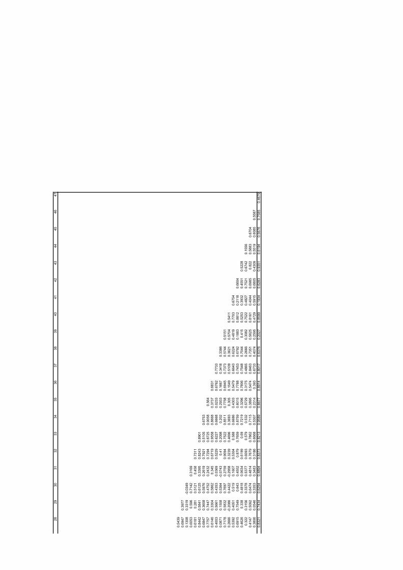
28

29

30

31

32

33

34

35

36

37

38

39

40

41

42

43

44

45

46

47

0.5

43

9

0.6

94

70

.39

77

0.1

30

80

.33

19

-0.0

34

9

0.6

05

30

.59

60

.71

42

0.3

16

9

0.6

18

10

.28

10

.51

21

0.4

58

0.7

31

1

0.8

44

20

.58

41

0.6

12

50

.33

95

0.8

24

30

.89

01

0.6

84

70

.36

58

0.5

97

60

.26

19

0.7

92

10

.51

05

0.6

75

3

0.7

75

70

.74

47

0.4

75

20

.24

32

0.7

29

40

.67

25

0.9

05

80

.56

4

0.6

14

60

.33

04

0.5

86

20

.34

50

.67

19

0.9

55

80

.86

68

0.3

73

70

.68

31

0.4

00

30

.56

61

0.4

35

30

.03

69

0.5

22

90

.62

27

0.6

66

80

.02

33

0.6

76

20

.77

33

0.0

87

10

.15

58

0.5

36

4-0

.07

43

0.4

10

.20

98

0.2

02

0.2

93

30

.16

67

0.3

41

80

.33

86

0.7

17

80

.58

32

0.7

69

70

.27

59

0.9

09

40

.75

22

0.8

51

10

.77

58

0.6

94

50

.73

73

0.5

74

40

.51

51

0.2

66

6-0

.20

86

0.4

42

2-0

.29

58

0.3

23

90

.46

96

0.3

69

30

.30

50

.15

49

0.5

10

90

.36

21

0.5

70

40

.54

11

0.5

39

20

.40

51

0.5

19

0.1

60

70

.53

04

0.5

88

0.6

68

60

.43

03

0.5

47

90

.66

43

0.6

22

40

.48

19

0.7

70

30

.67

54

0.6

91

50

.75

49

0.6

43

0.4

55

20

.87

90

.76

59

0.8

75

90

.60

15

0.7

78

80

.74

53

0.6

79

20

.18

83

0.8

81

20

.21

18

0.6

60

4

0.4

62

60

.33

80

.48

18

0.0

63

40

.61

99

0.6

90

.72

19

0.3

29

60

.78

06

0.7

54

80

.70

44

0.4

15

0.5

25

30

.39

32

0.4

55

10

.52

28

0.3

22

0.3

15

60

.33

78

0.5

37

70

.60

93

0.5

79

0.5

32

0.5

72

90

.31

75

0.4

86

50

.26

66

0.3

08

20

.75

22

0.4

82

70

.75

21

0.6

74

20

.15

56

0.4

14

70

.50

92

0.6

47

40

.48

14

0.7

67

90

.78

62

0.7

11

50

.38

95

0.5

47

40

.84

63

0.7

35

10

.56

25

0.8

16

10

.40

44

0.6

98

50

.82

20

.58

83

0.6

70

4

0.3

80

60

.05

46

0.3

35

30

.34

83

0.3

18

60

.66

68

0.5

30

70

.23

14

0.3

93

0.6

73

30

.40

74

0.2

59

50

.47

29

0.5

91

50

.68

05

0.4

30

90

.55

19

0.6

08

50

.55

87

0.8

32

10

.74

34

0.6

25

40

.48

94

0.8

37

30

.82

13

0.9

58

90

.66

77

0.8

91

40

.80

17

0.6

37

60

.20

27

0.8

59

90

.19

34

0.6

28

30

.93

51

0.6

19

40

.56

76

0.7

58

50

.46

79

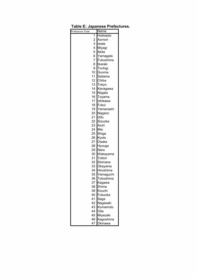
Table E: Japanese Prefectures.Name

1 Hokkaido

2 Aomori

3 Iwate

4 Miyagi

5 Akita

6 Yamagata

7 Fukushima

8 Ibaraki

9 Tochigi

10 Gunma

11 Saitama

12 Chiba

13 Tokyo

14 Kanagawa

15 Niigata

16 Toyama

17 Ishikawa

18 Fukui

19 Yamanashi

20 Nagano

21 Gifu

22 Sizuoka

23 Aichi

24 Mie

25 Shiga

26 Kyoto

27 Osaka

28 Hyougo

29 Nara

30 Wakayama

31 Tottori

32 Shimane

33 Okayama

34 Hiroshima

35 Yamaguchi

36 Tokushima

37 Kagawa

38 Ehime

39 Kouchi

40 Fukuoka

41 Saga

42 Nagasaki

43 Kumamoto

44 Oita

45 Miyazaki

46 Kagoshima

47 Okinawa