The Influence of Highways on Rural Economic Development...

Haskins

1

The Influence of Highways on Rural Economic Development: Evidence from North Carolina

By:

Conaway B. Haskins III

A Masters Project submitted to the faculty of the University of North Carolina at Chapel Hill

in partial fulfillment of the requirements for the degree of Master of Regional Planning

in the Department of City and Regional Planning. Chapel Hill 2002 Approved By: _________________________ ___________________________ READER (optional) ADVISOR

Haskins

2

Introduction

State and local highway investment projects are often justified on grounds that

such efforts will produce positive economic impacts. In particular, road network

enhancements are trumpeted as a primary means of bringing development to distressed

areas, including rural localities. In some manner, transportation routes have been

promoted as vehicles for commerce in the U.S. For rural areas experiencing economic

distress, such policies are often welcomed with open arms. Empirical evidence suggests

that there is a relationship between the presence of major highways and economic

development in general, however, evidence is less certain as to whether road investments

play a role in the economic growth of rural areas specifically.

Spurred by the initiation of the “Good Roads State” policy in the 1920’s, the state

of North Carolina began an ambitious effort to connect every county seat and major

locality in the state with a state highway (Harrington 1989). Where possible, these roads

were four-lanes highways. Often, they ran though low-density rural areas. Even though

the construction of these state highways is virtually complete, there is still a move within

policy circles for increasing the state’s highway capacity in order to spur rural

development (Rural Task Force 2000). Despite the prevalence of research on the subject

of rural economic development and transportation, the current effects of North Carolina’s

highway system on rural economies is less certain. Much of the state’s current road

network was built out by the 1960’s, but roadway lane expansions and interstate highway

extensions have been made since and are planned for the future. Despite the massive road

system, rural development advocates continue to cite highway expansion as a major

Haskins

3

mechanism for economic development. This paper seeks to determine if highway

investments are an enabler of economic development in rural North Carolina.

Building off of the recent convergence of rural transportation and economic

development policy in North Carolina, the paper examines if, given the widespread

coverage of the state road network, highway investment – in terms of mileage - is a

differentiating development factor among rural counties. This research is motivated by

several factors. As previously asserted, transportation projects, including highways, are

often justified based upon expected and potential economic development impacts. North

Carolina has historically shown a preference for highway infrastructure development and

improvements over alternative forms of transportation. The justification for such a

system, The Good Roads State Policy, was partially based upon perceived economic

benefits, including job growth. The paper will test if transportation infrastructure

influences economic development in North Carolina, a state that has a dispersed and

dense road system and a significant non-agricultural economy. It will also establish

whether marginal accessibility benefits, in terms of jobs, accrue to a state with a mature

road system.

The Policy Context: Good Roads and Economic Development

Transportation issues have been at the forefront of North Carolina’s state

government’s efforts to bring prosperity to its people and communities since North

Carolina’s inception. In particular, over the last eighty years, the development of

highways has been a key component to the economic development and growth policies

instituted by the state and its counties. More recently, issues of the rural economic

Haskins

4

development and rural transportation have converged, thus giving rise to discussions that

mirror those of the days prior to the Good Roads Policy (Rural Task Force 2001).

In 1915, the state legislature authorized the formation of an active Highway

Commission to oversee the state’s roadway investments. The Commission consisted of

several high-profile individuals who were very interested in growing the state’s economy

through transportation. Based upon their efforts, the state government in partnership with

the counties began an ambitious road construction project. From this effort, North

Carolina earned the nickname of “The Good Roads State.” With the devastating effects of

the Great Depression at hand, the state assumed responsibility of providing roads for the

counties. Since that time, county roads were, have been state roads. The system was

divided among a combination of multilane freeways, primary arterial highways, and

secondary, local-serving routes (Harrington 1989).

After weathering the Depression and World War II, the state developed a stable

highway finance fund for constructing highways, and continues to do so to this day.

During the 1950’s the federal Interstate Highway Act provided additional roadways to

states, and North Carolina developed its portion of the interstate system, guiding the

creation of several routes throughout it. The federal system further increased the highway

network, and the bulk of the state and interstate highway system was completed by 1990

with the completion of I-40 from Raleigh to Wilmington (Harrington 1989). Currently,

the state contains of over 78,000 miles of highways, and all but 7 counties contain part of

the state highway and interstate system (NC DOT 2000).

A prime example of the convergence of rural transportation and development

planning and policy is the creation and administration of Rural Planning Organizations

Haskins

5

(RPOs). In 1999, the General Assembly passed legislation authorizing the creation of

(RPOs), and charged the state Department of Transportation (NC DOT) with

implementing the program. RPOs are voluntary organizations that work cooperatively

with the Department to plan rural transportation systems and to advise the state

government on rural transportation policy (NC DOT 2001). RPOs have several required

functions that can be accentuated by other activities as regions see fit. Other planning-

related activities may stem from formation of an RPO, as they relate to integrating multi-

modal transportation planning with regionalism. The legislation allows for the

combination of transportation, land use and economic development activities, and RPO

advocates have advanced the notion that integrating transportation and economic

development will enhance the economies of rural counties.

Another example of this convergence rests with the establishment of the Rural

Prosperity Task Force. The state created the Rural Prosperity Task Force to address the

destructive effects of natural disasters (such as Hurricane Floyd), the decline of the

textiles industry, and the recent developments in the tobacco industry. The Task Force

works under the premise that rural North Carolina counties face certain challenges and

pressures that converged to cause a sense of distress. Statewide, the overall economy was

growing yet thousands of rural manufacturing workers were being laid off and the

traditional tobacco-focused agricultural economy was facing a crisis status. The task

force determined that much of rural North Carolina lacked the appropriate infrastructure

to connect to the emerging, growing global economy (Rural Task Force 2000). Among its

recommendations are proposals for increased funding for transportation projects in rural

counties. The central tenet of the task force recommendation is the establishment of

Haskins

6

policies and funds for joint rural transportation and economic development program to

implement road improvements that increase economic development opportunities (Rural

Task Force 2000).

The final prime example of the integration of rural transportation and economic

development concerns is a major report developed by the Brookings Institution. Along

with the state policy efforts, the Brookings Institution (2000) compiled a large amount of

data to study growth patterns across the state of North Carolina and performed trend

analysis. They found that North Carolina has enjoyed significant population and

economic growth throughout the 1990s, and it is one of the fastest growing states in the

nation. Over the past decade, North Carolina has become attractive for migrants due to its

relative high quality of life. However, the factors that make it a desirable and growing

location threaten the long-term health of the state due to rapid growth. North Carolina is

growing at a rapid pace in terms of population, jobs and land consumption. Most of this

growth occurs in the state’s seven major metro areas, and urban and suburban sprawl

threatens the quality of life of many parts of NC. Mainly occurring in major metro area,

rapid growth is not uniform over the entire state. Brookings holds that rural North

Carolina, as a whole, has not recently undergone the same rapid growth patterns as

metropolitan North Carolina, and those rural areas are not currently seeing the benefits

related to job growth that the states metropolitan areas are. One caveat is that this study

view rural counties in total, and did not differentiate between counties with growth and

those that have historically had distressed economies.

Brookings concludes that North Carolina needs to enact policies and practices to

purse a different growth pattern toward more compact and balanced areas. Among the

Haskins

7

eight steps that they recommend is rethinking state and local transportation policy to

counteract the historic over-investment in highways. They propose alternative

transportation strategies and a continuing support of rural economic development efforts.

Given the current and historical policy environment, the issue of transportation as

a mechanism to further rural economic development is of great importance. This

convergence of two streams of policy has significant implications for the future of rural

North Carolina and the state in general. Additionally, the decentralized road network of

North Carolina is a unique case for testing whether accessibility improvements of

highways in a state with ubiquitous road access has any economic development impacts.

The Literature

The empirical literature linking transportation to economic variables is rich in

scope and scale. Analysts and researches have sought to link transportation improvements

with economic grown and development. A prime argument is that transportation, rather

than crowd out private investment (such as other public expenditures are held to do),

actually stimulates investment, and thus economic activity, by increasing the rates of

return to private capital (Banister and Berechman 2000). This empirical work has sought

to advance the notion that there are significant and positive correlations between highway

transportation infrastructure and economic activity (Apogee 1994). Many empirical

studies assert that transportation infrastructure is important in generating local economic

development (e.g., Brown, 1999, Cambridge Systematics et al., 2001, and Forkenbrock

and Foster, 1996).

Haskins

8

Others view transportation as a necessary, but not sufficient, condition for

economic growth (Eberts 1990). Others find that highway systems interact with other

variables to drive rural economic growth (Aldrich and Kusmin 1997). Some assert that

other factors are sometimes found to be more important than highways for generating

benefits (Brown 1999). These other factors include an area’s attractiveness to retirees, the

presence of right-to-work laws, excellent high school completion rates, and good public

education expenditures. Poor earnings growth was due to higher wage levels, high

concentrations of transfer-payment recipients, and concentrations of small, independent

businesses in goods-producing sectors.

Empirical research also suggests that geographical proximity to metropolitan

areas plays an important role in growth outcomes along with other factors. Thus,

urbanization, development, and public infrastructure may be important triggering forces

in the US. Economic growth of counties with interstate highways is greatest for those

close to large cities or those with some degree of prior urbanization. Interstate counties

that are isolated or rural have few benefits over different periods of time (Rephann and

Isserman 1994).

Other research has shown unique links between transportation and economic

development, often at an industrial level. New manufacturing location is systematically

influenced by the provision of highway infrastructure. The development of new

motorways affects the spatial allocation of new manufacturing establishments at the

municipal level, and some evidence indicates that negative spillover effects may occur in

terms of displacement of current industrial centers. There is evidence that that

manufacturing firms prefer locations closer to new highways to the detriment of more

Haskins

9

distant municipalities that are not connected (Holl 2001). Certain empiricists conclude

that finds that negative spillover effects are shown to exist in the case of street-and-

highway capital. They assert that changes in county output are positively associated with

changes in street-and-highway capital within the same county, but output changes are

negatively associated with changes in street-and-highway capital in other counties

(Boarnet 1998). Thus, in some instances increasing highway capacity can actually

displace employment and economic activity versus generating new activity. Still, the

literature is not conclusive.

Increases in four-lane highways, interstate access, and two-lane highway density

have also been found to stimulate new manufacturing firm employment. Those regions

that consistently have higher-than average employment density (a proxy for

agglomeration economies) influence employment gains in other areas as well. A major

implication for state and local policymakers is that the location, timing, and type of

highway investment matter concerning whether highway investment serves as an

economic development aid not just the shear production of those highways. (Singletary

1995)

Some authors find that find that highways have differential impact across

industries. Thus, certain industries will grow as a result of reduced transportation costs,

while others contract as economic activity relocates. As with manufacturing, highways

affect the spatial allocation of general economic activity. However, while highways raise

the level of economic activity in the counties that they pass directly through, those roads

draw activity away from adjacent counties without interstates (Chandra and Thompson

2000). As for labor, transportation accessibility is still considered important to the

Haskins

10

economic fortunes of workers. A relationship exists between accessibility and economic

opportunity. Studies indicate that limitations on access experienced by certain workers do

affect labor market outcomes. Though other factors come into play, transportation

accessibility plays a significant role in advancing economically (O’Regan and Quigley

1999).

In some instances, variations in affects are due to differences in areas. Some non-

metro interstate interchanges often vary according to different functions that they

perform, with others some acting as interchange villages, performing the role of central

places in their regions (Moon 1988).The differentials are due to the remoteness and

isolation of the areas themselves more so than the actual highway. And, there is some

indication that highways are losing their influence on the economic development of an

area. This line of inquiry concludes that access to highways generally has become a less

important factor in location decisions than it was earlier. State-level highway investment

policies that emphasize proper maintenance and relatively minor improvements are likely

to be more cost-effective strategies for economic development than expensive highway

construction projects (Forkenbrock and Foster 1996).

The literature on transportation role in rural economic development leads to

interesting findings. Though differences do exist between the implicit and explicit and

positive and negative impacts and effects of highways on rural areas, evidence suggests

that road infrastructure has an influence on rural economic development. Highways are

either a primary or secondary economic mover. In consort with other productivity and

cost factors or alone, roads tend to serve as producers or inhibitors rural economic

development.

Haskins

11

However, there are several major shortcomings of the literature. Empirical

research fails to sufficiently account for the degree of highway accessibility that is

necessary to generate rural economic development. The research also does not account

for wide-scale development differential between areas of the same state or region. Rather,

the studies either consider data from large grouping of rural areas or with specific

segments of a roadway. Also, the research does not account for whether enhancements to

mature road systems generate any benefits whatsoever.

Given the findings of the above literature and the state of highway infrastructure

in North Carolina, this paper hypothesizes that highway infrastructure does not

significantly influence rural economic development, on a county level, in areas with a

dispersed and dense highway system. Given that highways are rather ubiquitous in the

state, transportation is not a scarce good. The high volume of roadways virtually

eliminates resource price differentials because the cost of access to firms is zero. As such,

good highway access is not particularly valuable to business and does not influence

location decisions. If these assumptions hold, further increasing that infrastructure will

not longer be a significant economic growth generator. Thus, North Carolina’s highway

system will not influence rural economic development.

Haskins

12

Methods and Data

Economic development is a function of a variety of costs and production factors,

including transportation. The literature highlighted several of these factors. The most

notable one were market size, localization and urbanization economies, local costs

factors, labor cost qualifications, the business cycles, and transportation accessibility

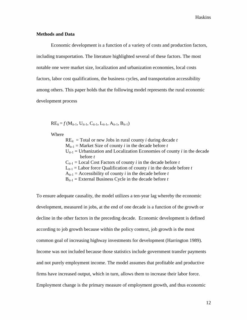
among others. This paper holds that the following model represents the rural economic

development process

REit = f (Mit-1, Uit-1, Cit-1, Lit-1, Ait-1, Bit-1)

Where

REit = Total or new Jobs in rural county i during decade t Mit-1 = Market Size of county i in the decade before t Uit-1 = Urbanization and Localization Economies of county i in the decade

before t Cit-1 = Local Cost Factors of county i in the decade before t Lit-1 = Labor force Qualification of county i in the decade before t Ait-1 = Accessibility of county i in the decade before t Bit-1 = External Business Cycle in the decade before t

To ensure adequate causality, the model utilizes a ten-year lag whereby the economic

development, measured in jobs, at the end of one decade is a function of the growth or

decline in the other factors in the preceding decade. Economic development is defined

according to job growth because within the policy context, job growth is the most

common goal of increasing highway investments for development (Harrington 1989).

Income was not included because those statistics include government transfer payments

and not purely employment income. The model assumes that profitable and productive

firms have increased output, which in turn, allows them to increase their labor force.

Employment change is the primary measure of employment growth, and thus economic

Haskins

13

development, for this research. Several different employment measures are included to

account for shifts in sector employment in the areas. Total and new employment is used

to measure the overall effects of economic development. Manufacturing employment is

used to capture the specialization that may be increasing or declining within an economy.

Finally, Private, Non-Farm employment is used to measure the effects within the

commercial labor economy.

Market size provides firms with labor resources, thus greater population leads to a

greater market size for labor. Population statistics are the measures of market size.

Localization and urbanization economies are the result of relative specializations of an

area’s business sector and population density. Location quotients indicate potential

competitive advantages of the firms and sectors in an area due to specialization.

Population density highlights the level of urbanization of the residents of a county. Local

cost factors vis-à-vis jobs are measured in terms of wage rates. Given the focus on

employment as a measure of development, including wage rates is sensible.

Labor force qualification is measured in terms of the percentage of an area’s adult

population that has attained either a high school diploma or a college diploma. Although

other determinants of qualification exist, the limitations of data in terms of consistency

influence the decision to use these two variables as factors. Accessibility measures the

ease through which labor can access employment opportunities. Geographic access to

high-employment areas and transportation access are assumed to play important roles in

employment levels, and thus are used to measure this. Finally, firm decisions are made

with respect to the national economy, and this affects their ability to provide labor

opportunities. Thus, Gross Domestic Product is the indicator for national business cycle.

Haskins

14

Data were collected at the county level in ten-year increments for decades

between 1970 and 2000 (with population data collected for 1960) for each of the factors

except GDP, which is a national statistic. For this paper, the unit of analysis is the

county. Designation as rural is determined by inclusion in a Metropolitan Statistical Area

(MSA) during the 1970 Census. Those counties not in MSAs in 1970 are rural, and the

other counties are considered urban. The result is that, over time, some counties that were

rural in 1970 are currently urban due to inclusion in previously designated MSA or from

becoming new MSAs.

The US Office of Management and Budget designates MSAs for Federal

statistical purposes. The general concept of a metropolitan area is that of a geographic

area consisting of a large population nucleus together with adjacent communities having

a high degree of economic and social integration with the nucleus. MSA designation was

chosen in order to standardize measurement over time and across geographies. Since

economic activity does not explicitly recognize county borders, MSA designation

provided the best way to ensure the capture of most regional economic effects. Though

growth occurs in some instances without respect to political jurisdiction, policy decisions

are made within the framework of municipalities. Therefore, the factors influencing

development are functions of county borders. Finally, the MSA standard is applied

throughout the United States, thus it allows for application of this model and research in

other states.

Haskins

15

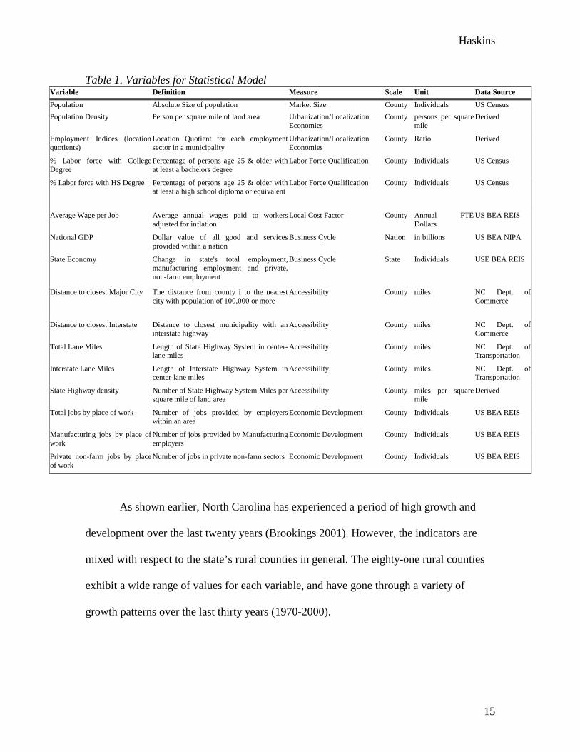
Table 1. Variables for Statistical Model Variable Definition Measure Scale Unit Data Source Population Absolute Size of population Market Size County Individuals US Census Population Density Person per square mile of land area Urbanization/Localization

Economies County persons per square

mile Derived

Employment Indices (location quotients)

Location Quotient for each employment sector in a municipality

Urbanization/Localization Economies

County Ratio Derived

% Labor force with College Degree

Percentage of persons age 25 & older with at least a bachelors degree

Labor Force Qualification County Individuals US Census

% Labor force with HS Degree Percentage of persons age 25 & older with at least a high school diploma or equivalent

Labor Force Qualification County Individuals US Census

Average Wage per Job Average annual wages paid to workers adjusted for inflation

Local Cost Factor County Annual FTE Dollars

US BEA REIS

National GDP Dollar value of all good and services provided within a nation

Business Cycle Nation in billions US BEA NIPA

State Economy Change in state's total employment, manufacturing employment and private, non-farm employment

Business Cycle State Individuals USE BEA REIS

Distance to closest Major City The distance from county i to the nearest city with population of 100,000 or more

Accessibility County miles NC Dept. of Commerce

Distance to closest Interstate Distance to closest municipality with an interstate highway

Accessibility County miles NC Dept. of Commerce

Total Lane Miles Length of State Highway System in center-lane miles

Accessibility County miles NC Dept. of Transportation

Interstate Lane Miles Length of Interstate Highway System in center-lane miles

Accessibility County miles NC Dept. of Transportation

State Highway density Number of State Highway System Miles per square mile of land area

Accessibility County miles per square mile

Derived

Total jobs by place of work Number of jobs provided by employers within an area

Economic Development County Individuals US BEA REIS

Manufacturing jobs by place of work

Number of jobs provided by Manufacturing employers

Economic Development County Individuals US BEA REIS

Private non-farm jobs by place of work

Number of jobs in private non-farm sectors Economic Development County Individuals US BEA REIS

As shown earlier, North Carolina has experienced a period of high growth and

development over the last twenty years (Brookings 2001). However, the indicators are

mixed with respect to the state’s rural counties in general. The eighty-one rural counties

exhibit a wide range of values for each variable, and have gone through a variety of

growth patterns over the last thirty years (1970-2000).

Haskins

16

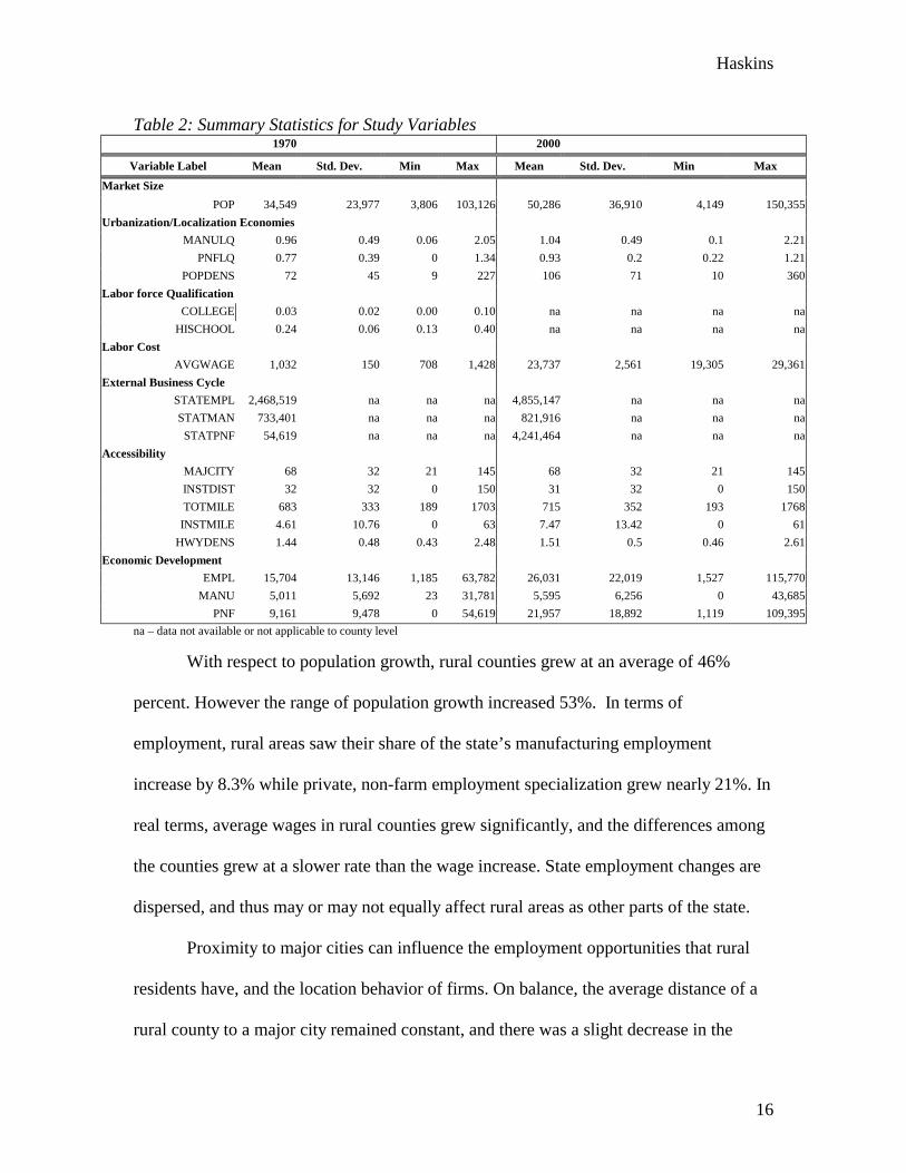
Table 2: Summary Statistics for Study Variables 1970 2000

Variable Label Mean Std. Dev. Min Max Mean Std. Dev. Min Max Market Size

POP 34,549 23,977 3,806 103,126 50,286 36,910 4,149 150,355 Urbanization/Localization Economies

MANULQ 0.96 0.49 0.06 2.05 1.04 0.49 0.1 2.21 PNFLQ 0.77 0.39 0 1.34 0.93 0.2 0.22 1.21

POPDENS 72 45 9 227 106 71 10 360 Labor force Qualification

COLLEGE 0.03 0.02 0.00 0.10 na na na na HISCHOOL 0.24 0.06 0.13 0.40 na na na na

Labor Cost AVGWAGE 1,032 150 708 1,428 23,737 2,561 19,305 29,361

External Business Cycle STATEMPL 2,468,519 na na na 4,855,147 na na na STATMAN 733,401 na na na 821,916 na na na

STATPNF 54,619 na na na 4,241,464 na na na Accessibility

MAJCITY 68 32 21 145 68 32 21 145 INSTDIST 32 32 0 150 31 32 0 150 TOTMILE 683 333 189 1703 715 352 193 1768

INSTMILE 4.61 10.76 0 63 7.47 13.42 0 61 HWYDENS 1.44 0.48 0.43 2.48 1.51 0.5 0.46 2.61

Economic Development EMPL 15,704 13,146 1,185 63,782 26,031 22,019 1,527 115,770

MANU 5,011 5,692 23 31,781 5,595 6,256 0 43,685 PNF 9,161 9,478 0 54,619 21,957 18,892 1,119 109,395

na – data not available or not applicable to county level

With respect to population growth, rural counties grew at an average of 46%

percent. However the range of population growth increased 53%. In terms of

employment, rural areas saw their share of the state’s manufacturing employment

increase by 8.3% while private, non-farm employment specialization grew nearly 21%. In

real terms, average wages in rural counties grew significantly, and the differences among

the counties grew at a slower rate than the wage increase. State employment changes are

dispersed, and thus may or may not equally affect rural areas as other parts of the state.

Proximity to major cities can influence the employment opportunities that rural

residents have, and the location behavior of firms. On balance, the average distance of a

rural county to a major city remained constant, and there was a slight decrease in the

Haskins

17

distance of rural counties to an interstate highway. Distance to interstates is considered

because the literature showed that interstates have varying effects on localities. Nearby

interstates can enhance a counties’ economy, while being further from interstates may

contribute to decline. On average, rural counties have less than 5% more state highway

miles and highway density over the 30-year period, but those counties saw their interstate

mileage increase by over 62%.

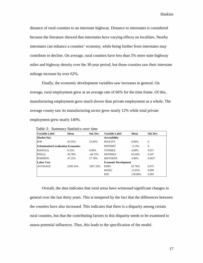
Finally, the economic development variables saw increases in general. On

average, rural employment grew at an average rate of 66% for the time frame. Of this,

manufacturing employment grew much slower than private employment as a whole. The

average county saw its manufacturing sector grow nearly 12% while total private

employment grew nearly 140%.

Table 3: Summary Statistics over time Variable Label Mean Std. Dev. Variable Label Mean Std. Dev. Market Size Accessibility POP 45.55% 53.94% MAJCITY 0.00% 0

Urbanization/Localization Economies INSTDIST -3.13% 0 MANULQ 8.33% 0.00% TOTMILE 4.69% 0.057 PNFLQ 20.78% -48.72% INSTMILE 62.04% 0.247 POPDENS 47.22% 57.78% HWYDENS 4.86% 0.0417 Labor Cost Economic Development AVGWAGE 2200.10% 1607.33% EMPL 65.76% 0.675 MANU 11.65% 0.099 PNF 139.68% 0.993

Overall, the data indicates that rural areas have witnessed significant changes in

general over the last thirty years. This is tempered by the fact that the differences between

the counties have also increased. This indicates that there is a disparity among certain

rural counties, but that the contributing factors to this disparity needs to be examined to

assess potential influences. Thus, this leads to the specification of the model.

Haskins

18

The Model and Empirical Results

Recall that a model has been hypothesized using several factors that empirical

research has shown as affecting economic development, such as market size,

agglomeration economies, local cost factors, labor force qualifications, accessibility, and

the external business cycle. Using OLS regression, two sets of models are developed, in

which highway access is factored with the other variables and tested with respect to

employment changes. Each set of models contains three specifications. The first set uses

total employment, manufacturing employment, and private, non-farm employment as

dependent variables. It seeks to account for differences between the total stocks of

independent variables among the counties. The second set uses changes in total

employment, manufacturing employment and private, non-farm employment (lagged).

This approach accounts for differences in the changes among the counties over time.

Both models incorporate time dummies for 1990 and 2000 in order to account for time-

series effects.

Models with Employment Totals

The first specification, using manufacturing employment as a dependent variable,

accounts for at least 79.4% of the variation in the outputs. Of the independent variables,

eight demonstrate at least 90% significance. This iteration indicates that differences in

manufacturing employment are positively linked to total highway mileage, population

density, distance to interstate highways, and specialization in manufacturing. Highway

density, population, and the average wage per job appear to account for negative changes

in manufacturing employment. These results indicate that areas further away from

Haskins

19

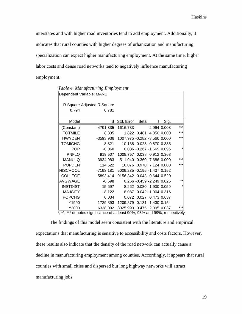
interstates and with higher road inventories tend to add employment. Additionally, it

indicates that rural counties with higher degrees of urbanization and manufacturing

specialization can expect higher manufacturing employment. At the same time, higher

labor costs and dense road networks tend to negatively influence manufacturing

employment.

Table 4. Manufacturing Employment Dependent Variable: MANU

R Square Adjusted R Square

0.794 0.781

Model B Std. Error Beta t Sig. (Constant) -4791.835 1616.733 -2.964 0.003 *** TOTMILE 8.835 1.822 0.481 4.850 0.000 *** HWYDEN -3593.936 1007.975 -0.282 -3.566 0.000 *** TOMICHG 8.821 10.138 0.028 0.870 0.385

POP -0.060 0.036 -0.267 -1.669 0.096 * PNFLQ 919.507 1008.757 0.038 0.912 0.363

MANULQ 3934.983 511.940 0.360 7.686 0.000 *** POPDEN 114.522 16.076 0.970 7.124 0.000 ***

HISCHOOL -7198.181 5009.235 -0.195 -1.437 0.152 COLLEGE 5893.414 9156.342 0.043 0.644 0.520

AVGWAGE -0.598 0.266 -0.459 -2.249 0.025 ** INSTDIST 15.697 8.262 0.080 1.900 0.059 * MAJCITY 8.122 8.087 0.042 1.004 0.316 POPCHG 0.034 0.072 0.027 0.473 0.637

Y1990 1729.893 1209.879 0.131 1.430 0.154 Y2000 6338.092 3025.993 0.475 2.095 0.037 ***

*, **, *** denotes significance of at least 90%, 95% and 99%, respectively

The findings of this model seem consistent with the literature and empirical

expectations that manufacturing is sensitive to accessibility and costs factors. However,

these results also indicate that the density of the road network can actually cause a

decline in manufacturing employment among counties. Accordingly, it appears that rural

counties with small cities and dispersed but long highway networks will attract

manufacturing jobs.

Haskins

20

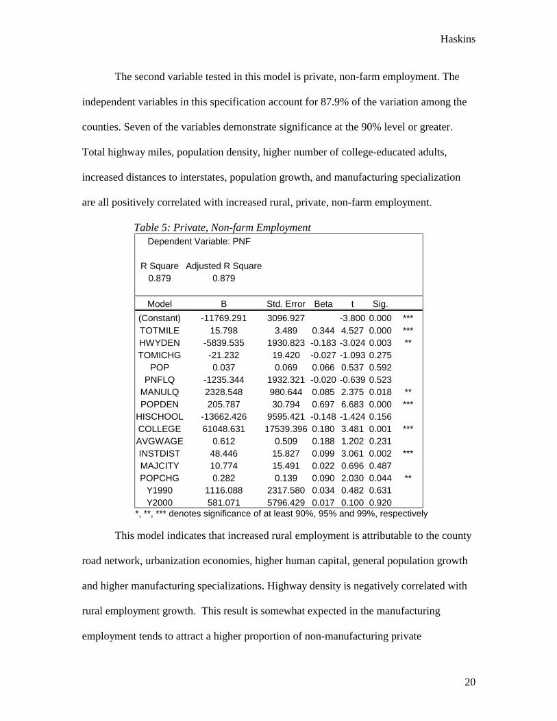
The second variable tested in this model is private, non-farm employment. The

independent variables in this specification account for 87.9% of the variation among the

counties. Seven of the variables demonstrate significance at the 90% level or greater.

Total highway miles, population density, higher number of college-educated adults,

increased distances to interstates, population growth, and manufacturing specialization

are all positively correlated with increased rural, private, non-farm employment.

Table 5: Private, Non-farm Employment Dependent Variable: PNF


0.879 0.879

Model B Std. Error Beta t Sig. (Constant) -11769.291 3096.927 -3.800 0.000 *** TOTMILE 15.798 3.489 0.344 4.527 0.000 *** HWYDEN -5839.535 1930.823 -0.183 -3.024 0.003 ** TOMICHG -21.232 19.420 -0.027 -1.093 0.275

POP 0.037 0.069 0.066 0.537 0.592 PNFLQ -1235.344 1932.321 -0.020 -0.639 0.523

MANULQ 2328.548 980.644 0.085 2.375 0.018 ** POPDEN 205.787 30.794 0.697 6.683 0.000 ***

HISCHOOL -13662.426 9595.421 -0.148 -1.424 0.156 COLLEGE 61048.631 17539.396 0.180 3.481 0.001 *** AVGWAGE 0.612 0.509 0.188 1.202 0.231 INSTDIST 48.446 15.827 0.099 3.061 0.002 *** MAJCITY 10.774 15.491 0.022 0.696 0.487 POPCHG 0.282 0.139 0.090 2.030 0.044 **

Y1990 1116.088 2317.580 0.034 0.482 0.631 Y2000 581.071 5796.429 0.017 0.100 0.920


This model indicates that increased rural employment is attributable to the county

road network, urbanization economies, higher human capital, general population growth

and higher manufacturing specializations. Highway density is negatively correlated with

rural employment growth. This result is somewhat expected in the manufacturing

employment tends to attract a higher proportion of non-manufacturing private

Haskins

21

employment. And unexpected finding is that increased distances from interstate increase

private, non-farm employment. A possible explanation is that those counties with the

other necessary factors for growth benefit from not having an interstate highway to

displace employment. For this variable, it appears that increased road network coverage

inhibits higher employment.

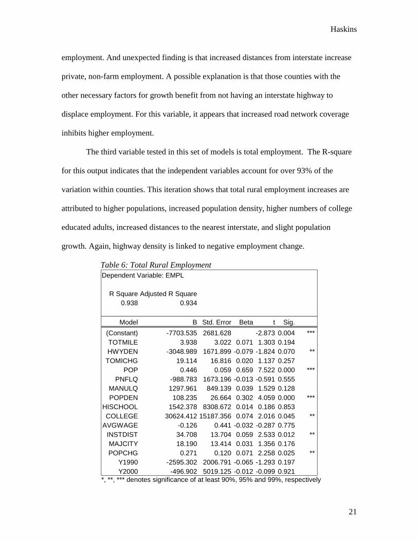
The third variable tested in this set of models is total employment. The R-square

for this output indicates that the independent variables account for over 93% of the

variation within counties. This iteration shows that total rural employment increases are

attributed to higher populations, increased population density, higher numbers of college

educated adults, increased distances to the nearest interstate, and slight population

growth. Again, highway density is linked to negative employment change.

Table 6: Total Rural Employment Dependent Variable: EMPL


0.938 0.934

Model B Std. Error Beta t Sig. (Constant) -7703.535 2681.628 -2.873 0.004 *** TOTMILE 3.938 3.022 0.071 1.303 0.194 HWYDEN -3048.989 1671.899 -0.079 -1.824 0.070 ** TOMICHG 19.114 16.816 0.020 1.137 0.257

POP 0.446 0.059 0.659 7.522 0.000 *** PNFLQ -988.783 1673.196 -0.013 -0.591 0.555

MANULQ 1297.961 849.139 0.039 1.529 0.128 POPDEN 108.235 26.664 0.302 4.059 0.000 ***

HISCHOOL 1542.378 8308.672 0.014 0.186 0.853 COLLEGE 30624.412 15187.356 0.074 2.016 0.045 **

AVGWAGE -0.126 0.441 -0.032 -0.287 0.775 INSTDIST 34.708 13.704 0.059 2.533 0.012 ** MAJCITY 18.190 13.414 0.031 1.356 0.176 POPCHG 0.271 0.120 0.071 2.258 0.025 **

Y1990 -2595.302 2006.791 -0.065 -1.293 0.197 Y2000 -496.902 5019.125 -0.012 -0.099 0.921


Haskins

22

Of particular interest is the impact that increased numbers of adults with college

degrees has on overall employment differentials among counties. The results suggest that

simply increasing the total of college-educated adults by one percent causes a difference

of over 30,000 jobs. Additionally, the results for interstate distance are unexpected in that

as a county moves away from an interstate, it gains employment with respect to other

counties. Finally, it is notable that highway miles and highway mile changes are not

significant in this model. Thus, there doesn’t seem to be a strong link between lane miles

and total employment in rural counties.

Models with Employment Change

The first model in this set tested manufacturing change. The battery of

independent variables in this model only account for 14% of the variation among

observations as demonstrated by the R-square of .196. For this iteration, three of the

coefficients tested as significant above 90%. This iteration indicates that slight increases

in total highway miles and population provide for manufacturing employment growth in

rural counties. It also appears that higher wages per job contribute to a decline in

manufacturing employment. Thus, a slight population and road growth coupled with low

wages may help foster change in rural manufacturing employment.

Of particular interest for this model is that there are so few independent variables

that demonstrate any level of statistical significance. That being said, the results for

accessibility and labor cost are expected; as accessibility increases and total wages

decrease, manufacturing employment grows. This is consistent with previous findings

and the hypothesis.

Haskins

23

Table 7: Change in Manufacturing Employment Dependent Variable: MANUCHG


0.196 0.142

Model B Std. Error Beta t Sig. (Constant) 741.826 708.287 1.047 0.296 TOTMILE 1.498 0.798 0.368 1.877 0.062 ** HWYDEN -678.867 441.592 -0.240 -1.537 0.126 TOMICHG 2.660 4.442 0.038 0.599 0.550

POP -0.023 0.016 -0.468 -1.476 0.141 PNFLQ -315.691 441.934 -0.059 -0.714 0.476

MANULQ 295.427 224.280 0.122 1.317 0.189 POPDEN 10.128 7.043 0.387 1.438 0.152

HISCHOOL 207.161 2194.534 0.025 0.094 0.925 COLLEGE 2922.006 4011.372 0.097 0.728 0.467

AVGWAGE -0.281 0.116 -0.974 -2.412 0.017 ** INSTDIST -1.279 3.620 -0.030 -0.353 0.724 MAJCITY 1.916 3.543 0.045 0.541 0.589 POPCHG 0.056 0.032 0.201 1.760 0.080 **

Y1990 -14.929 530.045 -0.005 -0.028 0.978 Y2000 1518.818 1325.680 0.513 1.146 0.253


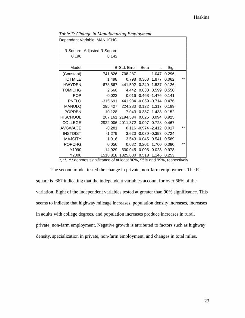
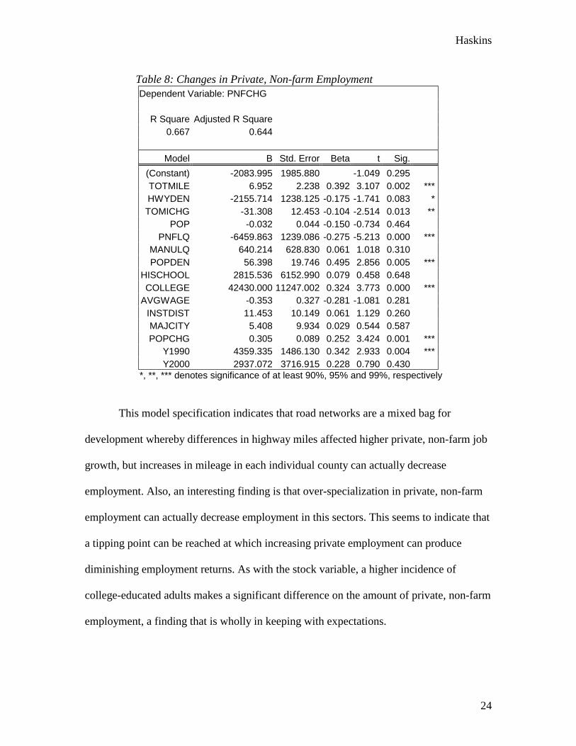
The second model tested the change in private, non-farm employment. The R-

square is .667 indicating that the independent variables account for over 66% of the

variation. Eight of the independent variables tested at greater than 90% significance. This

seems to indicate that highway mileage increases, population density increases, increases

in adults with college degrees, and population increases produce increases in rural,

private, non-farm employment. Negative growth is attributed to factors such as highway

density, specialization in private, non-farm employment, and changes in total miles.

Haskins

24

Table 8: Changes in Private, Non-farm Employment Dependent Variable: PNFCHG


0.667 0.644

Model B Std. Error Beta t Sig. (Constant) -2083.995 1985.880 -1.049 0.295 TOTMILE 6.952 2.238 0.392 3.107 0.002 *** HWYDEN -2155.714 1238.125 -0.175 -1.741 0.083 * TOMICHG -31.308 12.453 -0.104 -2.514 0.013 **

POP -0.032 0.044 -0.150 -0.734 0.464 PNFLQ -6459.863 1239.086 -0.275 -5.213 0.000 ***

MANULQ 640.214 628.830 0.061 1.018 0.310 POPDEN 56.398 19.746 0.495 2.856 0.005 ***

HISCHOOL 2815.536 6152.990 0.079 0.458 0.648 COLLEGE 42430.000 11247.002 0.324 3.773 0.000 ***

AVGWAGE -0.353 0.327 -0.281 -1.081 0.281 INSTDIST 11.453 10.149 0.061 1.129 0.260 MAJCITY 5.408 9.934 0.029 0.544 0.587 POPCHG 0.305 0.089 0.252 3.424 0.001 ***

Y1990 4359.335 1486.130 0.342 2.933 0.004 *** Y2000 2937.072 3716.915 0.228 0.790 0.430


This model specification indicates that road networks are a mixed bag for

development whereby differences in highway miles affected higher private, non-farm job

growth, but increases in mileage in each individual county can actually decrease

employment. Also, an interesting finding is that over-specialization in private, non-farm

employment can actually decrease employment in this sectors. This seems to indicate that

a tipping point can be reached at which increasing private employment can produce

diminishing employment returns. As with the stock variable, a higher incidence of

college-educated adults makes a significant difference on the amount of private, non-farm

employment, a finding that is wholly in keeping with expectations.

Haskins

25

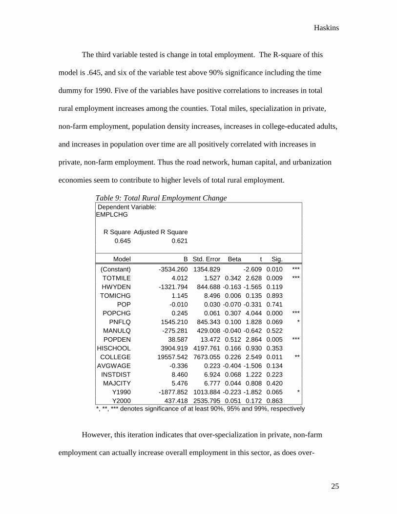
The third variable tested is change in total employment. The R-square of this

model is .645, and six of the variable test above 90% significance including the time

dummy for 1990. Five of the variables have positive correlations to increases in total

rural employment increases among the counties. Total miles, specialization in private,

non-farm employment, population density increases, increases in college-educated adults,

and increases in population over time are all positively correlated with increases in

private, non-farm employment. Thus the road network, human capital, and urbanization

economies seem to contribute to higher levels of total rural employment.

Table 9: Total Rural Employment Change Dependent Variable: EMPLCHG


0.645 0.621

Model B Std. Error Beta t Sig. (Constant) -3534.260 1354.829 -2.609 0.010 *** TOTMILE 4.012 1.527 0.342 2.628 0.009 *** HWYDEN -1321.794 844.688 -0.163 -1.565 0.119 TOMICHG 1.145 8.496 0.006 0.135 0.893

POP -0.010 0.030 -0.070 -0.331 0.741 POPCHG 0.245 0.061 0.307 4.044 0.000 ***

PNFLQ 1545.210 845.343 0.100 1.828 0.069 * MANULQ -275.281 429.008 -0.040 -0.642 0.522 POPDEN 38.587 13.472 0.512 2.864 0.005 ***

HISCHOOL 3904.919 4197.761 0.166 0.930 0.353 COLLEGE 19557.542 7673.055 0.226 2.549 0.011 **

AVGWAGE -0.336 0.223 -0.404 -1.506 0.134 INSTDIST 8.460 6.924 0.068 1.222 0.223 MAJCITY 5.476 6.777 0.044 0.808 0.420

Y1990 -1877.852 1013.884 -0.223 -1.852 0.065 * Y2000 437.418 2535.795 0.051 0.172 0.863


However, this iteration indicates that over-specialization in private, non-farm

employment can actually increase overall employment in this sector, as does over-

Haskins

26

saturation of highways. Additionally, as with other variables, increasing labor force

qualifications with respect to higher education seems to increase the incidence if rural

employment growth. As such, it is necessary to consider the mix of employment types

within a county in order to hedge against a trend toward over specialization. Finally, total

change in lane miles is not significant in this model, thus indicating the increasing

highway mileage in rural counties does not influence employment.

Implications and Conclusion

The models seem to indicate that a variety of factors play a role in rural

employment growth. Among these, population change, manufacturing specializations and

some degree of accessibility appear to be important factors. Different highway variables

played a role in development, yet, contrary to expectations, higher road mileage appears

to produce higher employment. However, the models consistently show that dense

highway networks in rural areas have negative employment effects. Thus, it can be

generalized that some degree of overall accessibility is necessary, but that too many roads

can be harmful to areas. Furthermore, the results of the models indicate that a tipping

point can be reached whereby increasing highways can produce diminishing employment

returns.

Among non-accessibility variables, the results of the models indicate that

increased labor force qualifications and dense population patterns contribute significantly

to employment growth in private employment and overall employment. In particular,

human capital and urbanization patterns, when coupled with increase distances from

interstates, foster growth within rural areas. This would indicate that those counties that

Haskins

27

urbanize are better able to control for displacement effects that interstate highways have

been shown to result it.

The empirical results have wide-ranging implications for a variety of policy actors

in transportation and rural economic development. For state-level transportation officials,

this research implies that focusing on enhancing the current road stock through lane-

width expansions and improvement may be a tool for increased economic development,

but that building additional highway miles may be detrimental to the creation of jobs.

Given the potentially high expense of increasing lane miles, the small number of

additional jobs attributed to lane mile enhancements may be a costly endeavor for the

state. The state may reconsider its funding and construction plans in order to produce the

desired economic impacts on a long-term basis as a justification for expenditures.

Advocating for additional lane miles is not supported by this research.

Economic development advocates and officials should also take caution in

continuing to advance the notion that more highways will automatically lead to more

development. It appears that highways contribute to accessibility in some measure, and

therefore, in tandem with other factors, like labor cost and human capital, help foster

rural growth and development. However, pushing for highway-specific infrastructure

development plans is not recommended.

State officials should also be mindful that labor force enhancements appear to

contribute significantly to rural development. Increasing workforce training and higher

education opportunities to rural residents will probably produce a greater impact on

economic outcomes that highways. A well-trained labor force stands to attract more

employment either through business growth and/or retention. Thus, connecting college

Haskins

28

attendance to employment is vital. At the same time, the state should not continue to

encourage low-wage labor as a development mechanism because non-farm employment

is inversely related to low wages. Continuing to guide localities into low-wage

employment opportunities could have a long-term deleterious effect.

The research also implies that local officials should take certain steps to bring

development to their rural areas and prevent negative growth. They should discontinue

the advocacy of more highways and try to develop better quality roads and possibly other

modes of transportation for individuals. Focusing on developing small cities or other

notes of commercial and residential life will probably enhance rural areas through

capturing urbanization and localization benefits. Local officials should also seek out

opportunities to develop higher education facilities in their counties. Finally, local

officials should not seek to attract employment via cheaper labor because this seems to

negatively correlate with non-manufacturing employment.

In general, the hypothesis that a mature road network - such as North Carolina’s –

does not produce additional benefits from increases lane-mile capacity appears to hold

true. As the literature indicated, transportation seems to be a contributor to economic

development under certain constructs. However, other factors, such as agglomeration

economies and labor force qualification have as much or more of an influence on

development variables, and appear to produce greater rural economic development.

Haskins

29

References

Aldrich, Lorna and Lorin Kusmin. 1997. Rural Economic Development: What Makes Rural Communities Grow? USDA Agriculture Information Bulletin No. 737. 7 pgs. Apogee Research, Inc. 1994. “The Economic Importance of the National Highway System” Prepared for Trucking Research Institute, Alexandria, VA Banister, D. and Berechman, J. (2000) Transport Investment and Economic Development. Chapter 6, University College-London Press, 131-160. Boarnet, Marlon G. 1998. Spillovers and the Locational Effects of Public Infrastructure. Journal of Regional Science. Vol. 38, No. 3, pp. 381-400. Brookings Institution. 2000. Adding It Up: Growth Trends and Policies in North Carolina. Center on Urban and Metropolitan Policy. 38 pgs. Brown, Dennis M. 1999. Highway Investment and Rural Economic Development: An Annotated Bibliography. Food and Rural Economics Division, Economic Research Service, US Dept. of Agriculture, No. 133. Cambridge Systematics, Inc. and Economic Development Research Group. 2001. Using Empirical Information to Measure the Economic Impact of Highway Investments. Prepared for: Federal Highway Administration. Chandra, Amitabh and Eric Thompson. 2000. “Does Public Infrastructure Affect Economic Activity? Evidence From the Rural Interstate Highway System.” Regional Science and Urban Economics. Vol. 30, pp. 457-490 Development. Transportation Research Record 1125. Eberts, Randall W. 1990. Public Infrastructure and Regional Economic Development, Economic Review, Federal Reserve Bank of Cleveland, Vol. 26, No. 1, pp. 15-27. Economic Development Quarterly Vol. 10 No. 3, August 1996. Forkenbrock, David J., and Norman S.J. Foster. Highways and Business Location Decisions. Gordon, Peter, Harry Richardson and Gang Yu. 1998. Metropolitan and Non-metropolitan Employment Trends in the US: Recent Evidence and Implications. Urban Studies, Vol. 35 No. 7, 1037-1057 Holl, Adelheid. 2001. Manufacturing Location and Impacts of Road Transport Infrastructure. The Case of Spain. NECTAR Conference no. 6: European Strategies in the Globalising Markets; Transport Innovations, Competitiveness and Sustainability in the Information Age.

Haskins

30

Moon, Henry E., Jr. 1988 Interstate Highway Interchanges as Instigators of Nonmetropolitan North Carolina Department of Commerce. Economic Development Scans. 2001. North Carolina Department of Transportation (NC DOT). Highway and Road Mileage: 1970-2000 North Carolina Department of Transportation. Rural Planning Organizations. 2001. North Carolina Rural Prosperity Task Force. 2000. Final Report O’Regan, K and J. Quigley. 1999. “Accessibility and Economic Opportunity” in Essays in Transportation Economics and Policy. Edited by J. Gomez-Ibanez et al. Washington, D.C., Brookings Institution Press, 437-466. Rephann, Terance J. 1993. Highway Investment and Regional Economic Development: Decision Methods and Empirical Foundations. Urban Studies, Vol. 30, No. 2, 437-450. Rephann, Terance J., and Andrew M. Isserman. 1994. New Highways as Economic Development Tools: An Evaluation Using Quasi-Experimental Matching Methods, Regional Science and Urban Economics, Vol. 24, No. 6, pp. 723-51. Singletary, Loretta, Mark Henry, Kerry Brooks, and James London. 1995. “The Impact of Highway Investment on New Manufacturing Employment in South Carolina: A Small Region Spatial Analysis” The Review of Regional Studies. Vol. 25, No. 1, 37-55 US Bureau of Economic Analysis. Regional Economic Information Systems. 1970-2000 US Bureau of the Census. Census of Population and Housing. General Social and Economic Characteristics: 1970-2000

The Influence of Highways on Rural Economic Development...

Documents

Transcript of The Influence of Highways on Rural Economic Development...