The impact of news on measures of undiversifiable risk: evidence from the UK stock market

Article

Accepted Version

Brooks, C. and Henry, O.T. (2002) The impact of news on measures of undiversifiable risk: evidence from the UK stock market. Oxford Bulletin of Economics and Statistics, 64 (5). pp. 487-507. ISSN 1468-0084 doi: https://doi.org/10.1111/1468-0084.00274 Available at http://centaur.reading.ac.uk/24149/

It is advisable to refer to the publisher’s version if you intend to cite from the work. See Guidance on citing .

To link to this article DOI: http://dx.doi.org/10.1111/1468-0084.00274

Publisher: Blackwell Publishing Ltd

All outputs in CentAUR are protected by Intellectual Property Rights law, including copyright law. Copyright and IPR is retained by the creators or other copyright holders. Terms and conditions for use of this material are defined in

the End User Agreement .

www.reading.ac.uk/centaur

CentAUR

Central Archive at the University of Reading

Reading’s research outputs online

This is the authors’ accepted manuscript of an article published in

the Oxford Bulletin of Economics and Statistics. The definitive

version is available at www3.interscience.wiley.com

2

The Impact of News on Measures of Undiversifiable

Risk: Evidence from the UK Stock Market*

Chris Brooks (corresponding author)

ISMA Centre, The University of Reading,

Whiteknights Park, PO Box 242, Reading RG6 6BA

United Kingdom.

Tel: +44 (0)118 9316768

Fax: +44 (0)118 9314741

E-Mail: c.brooks@ismacentre.rdg.ac.uk

Ólan T. Henry,

Department of Economics, University of Melbourne

Victoria 3010 Australia

Tel: + 613 3 8344 5312

Fax: +613 3 8344 6899

E-mail: oth@unimelb.edu.au

http://melbecon.unimelb.edu.au/staffprofile/ohenry/home.html

This Version: May 2002

Abstract

Using UK equity index data, this paper considers the impact of news

on time varying measures of beta, the usual measure of undiversifiable risk.

The empirical model implies that beta depends on news about the market and

news about the sector. The asymmetric response of beta to news about the

market is consistent across all sectors considered. Recent research is divided as

to whether abnormalities in equity returns arise from changes in expected

returns in an efficient market or over-reactions to new information. The

evidence suggests that such abnormalities may be due to changes in expected

returns caused by time-variation and asymmetry in beta.

JEL Codes: G12 G15

Keywords: Stock Index, Multivariate Asymmetric GARCH, News Impact Surfaces,

Conditional Beta Surfaces.

* Initial work on this paper took place while the second author was on study leave at the ISMA Centre,

The University of Reading. The News impact surfaces were graphed using a GAUSS Routine written

by the second author and Michalis Ioannides. The data and estimation routines are available upon

request from the corresponding author. We are indebted to Kalvinder Shields, seminar participants at

the University of Manchester and RMIT University and to an anonymous referee for helpful comments

on earlier drafts of this paper. The responsibility for any errors or omissions lies solely with the authors.

1

1. Introduction

There is widespread evidence that the volatility of equity returns is higher in bull

markets than in bear markets. One potential explanation for such asymmetry in variance is

the so-called 'leverage effect' of Black (1976) and Christie (1982). As equity values fall, the

weight attached to debt in a firm’s capital structure rises, ceteris paribus. This induces equity

holders, who bear the residual risk of the firm, to perceive the stream of future income

accruing to their portfolios as being relatively more risky.

An alternative view is provided by the 'volatility-feedback' hypothesis. Assuming

constant dividends, if expected returns increase when stock return volatility increases, then

stock prices should fall when volatility rises. Pagan and Schwert (1990), Nelson (1991),

Campbell and Hentschel (1992), Engle and Ng (1993), Glosten, Jagannathan and Runkle

(1993), and Henry (1998), inter alia, provide evidence of asymmetry in equity return

volatility using univariate GARCH models. Kroner and Ng (1995), Braun, Nelson and

Sunnier (1995), Henry and Sharma (1999), Engle and Cho (1999), and Brooks and Henry

(2000) inter alia use multivariate GARCH models to capture time-variation and asymmetry

in the variance-covariance structure of asset returns.

Such time-variation and asymmetry in volatility may be used to explain a time-

varying and asymmetric beta. A risk averse investor will trade off higher levels of expected

return for higher levels of risk. If the risk premium is increasing in volatility, and if beta is an

adequate measure of the sensitivity to risk, then time-variation and asymmetry in the

variance-covariance structure of returns may lead to time-variation and asymmetry in beta.

Recent research by Braun, Nelson and Sunnier (1995), hereafter BNS, explores time

variation and asymmetry in beta using a bivariate EGARCH model. Engle and Cho (1999),

hereafter EC, extend the BNS paper in two main directions. First, EC consider the differing

roles of market- and asset-specific shocks. This is important since a series of negative returns

caused by market or asset-specific shocks may lead to an increase in beta. Second, EC use

daily data on individual firms, rather than the aggregated data used by BNS.

2

Our approach differs from that of both BNS and EC. In particular we use a linear as

opposed to an exponential multivariate GARCH model to distinguish between the roles of

idiosyncratic and market shocks in determining potential asymmetry in beta. The exponential

GARCH approach of BNS does not readily admit negative covariance estimates although

such inverse relationships may be present in the data. Moreover, the EGARCH form appears

to overstate the response of the conditional variance to a negative shock - see Engle and Ng

(1993), and Henry (1998), inter alia. Our approach allows for a (potentially negative) time

varying and asymmetric covariance between the risky asset and market portfolio, while

guaranteeing a positive definite variance-covariance matrix. Moreover, we define the

Conditional Beta Surface, an extension of the News Impact Surface concept of Ng and

Kroner (1995). Using this approach it is possible to produce a graphical representation of the

impact of idiosyncratic and market-wide shocks upon estimates of beta. We also employ

indicator dummy regressions to identify sources of the observed asymmetry in the estimated

beta series. The models are applied in the context of the estimation of beta for six UK sector

return indices.

The remainder of the paper develops as follows. Section 2 outlines the strategy

employed for modelling the time-variation and asymmetry in beta, while section 3 describes

the data and presents the empirical results. The statistical properties of the estimated beta

series are reported in section 4. The final section of the paper provides a summary and some

concluding comments.

2. Modelling Time Variation and Asymmetry in Beta

The static Capital Asset Pricing Model (CAPM) predicts that the expected return to

investing in a risky asset or portfolio, E( tSR , ), should equal, fr , the risk free rate of return,

plus a risk premium. The risk premium is determined by a price of risk, the expected return

3

on the market portfolio in excess of fr , and a quantity of risk, known as the ‘beta’ of asset S,

S . The static CAPM may be written as

[ ( ) ]S f M f SE R r E R r (1)

where M and S denote the market and sector respectively,

,M S

S

M

Cov R R

Var R , and

, and M S MCov R R Var R are the covariance between the sector and market portfolio

returns and the variance of the market returns, respectively1.

Estimates of S may be obtained from OLS estimates of the slope coefficient in

, 0 1 ,S t M t tR b b R u (2)

It has long been recognised that the volatility of asset returns is clustered. Thus the

assumption of constant variance (let alone covariance) underlying the estimation of (2) must

be regarded as tenuous.

Let Et-1(.) represent the expectations operator conditional on information available at

time t-1. The conditional formulation of the Capital Asset Pricing Model (CAPM) predicts

that the expected return to investing in a risky asset or portfolio, Et-1(RS,t), should equal the

risk free rate of return plus a risk premium. The risk premium is determined by a price of risk,

Et-1(RM,t)-rf, and a quantity of risk, the beta of asset S, ,S t . This may be written as

)(var

),(cov])([)(

,

,,

,1,1

tMt

tMtSt

ftMtftStR

RRrRErRE (3)

where , , , ,cov / varS t t S t M t t M tR R R , and , ,covt S t M tR R and ,vart M tR are the

conditional covariance between the asset and market portfolio returns and the conditional

variance of the market returns respectively. Note that (3) assumes investors maximise utility

period by period and is written in terms of the conditional moments, reflecting market

1 The CAPM can be written as ,i f S ME R r COV R R , where is the market price per unit risk.

4

participants’ use of information available up to time 1t in making investment decisions for

time t . Unlike the static CAPM, (3) does not require constant S or constant risk premia.

The model presented by Merton (1973, 1980) predicts a positive relationship

between the market risk premium and the variance of the market portfolio. Bollerslev, Engle

and Wooldridge (1988), Braun, Nelson and Sunier (1995) and Engle and Cho (1999), inter

alia, report evidence of time variation in ,S t based upon the GARCH class of models.

Attanasio (1991), Engel, Frankel, Froot and Rodrigues (1995) and González-Rivera (1996)

present tests of the conditional CAPM allowing for predictability of the second moment of

asset returns. González-Rivera (1996) presents a testable version of the conditional CAPM

written as

),(cov)( ,,,1 tMtStftSt RRrRE (4)

where )(var/])([ ,, tMtftM RrRE represents the aggregate coefficient of relative risk

aversion and is assumed constant over time.

The focus of this paper is on the time series behaviour of ,S t and in particular

whether there is evidence of asymmetry in this measure of risk. Braun, Nelson and Sunnier

(1995) and Engle and Cho (1999) use the bivariate EGARCH approach specifying the

conditional mean equations as

, , ,

, , , , ,

M t M t M t

S t S t M t S t S t

R h z

R R h z

(5)

where , and M t S,tR R represent the demeaned returns to the market and sector respectively,

S,ttM zz and , are contemporaneously uncorrelated i.i.d. processes with zero mean and unit

variance and , and M t S,th h are the conditional variances of , and M t S,tR R , respectively. The

measure of undiversifiable risk associated with industry sector S, S, is defined as:

1 , ,

, 2

1 ,

[ ]

[ ]

t M t S t

S t

t M t

E R R

E R

(6)

5

where [.]1tE denotes the expectation at time t-1. The model is completed by the equations

defining the time series behaviour of S,ttStM hh and , ,,

1,31,21,1,101,40,

1,,1,1,1,,

1,1,1,,

)()()ln()ln(

)()ln()ln(

tStMtStMtStS

tMmMStSSStSSStSSStS

tMmMtMMMtMMMtM

zzzz

zgzgzhh

zgzhh

(7)

where 1,1,1, )( tititii zEzzg for i = M, S.

As noted by Braun et al. (1995), the bivariate EGARCH (7) implies some strong

assumptions. First, the model does not allow for feedback, as would be the case if

S,ttStM hh and )ln(),ln( ,, followed a VARMA process. Second, the model assumes a linear

autoregressive process for S,t . Third, although the model allows for leverage effects, it does

so in an ad-hoc fashion.

In contrast to Braun, Nelson and Sunnier (1995), and Engle and Cho (1999), our

approach allows for feedback between the conditional means and variances of tMR , and

tSR , . Furthermore, we make no formal assumptions as to the time series process underlying

S,t . We assume a VARMA process for the returns and model the time variation in the

variance-covariance matrix using a linear as opposed to an exponential GARCH model. The

multivariate GARCH approach allows the researcher to examine the effects of shocks to the

entire variance-covariance matrix. Thus the effect of a shock to tMR , on the covariance

between tMR , and tSR , may be inferred directly from the parameter estimates. Moreover, the

conditional variance-covariance matrix may be parameterised to be time varying and

asymmetric. Given the role of covariances in asset pricing and financial risk management,

correct specification of the variance-covariance structure is of paramount importance. For

example, the conditional covariance may be used in the calculation of prices for options

involving more than one underlying asset (such as rainbow options), and is vital to the

6

calculation of minimum capital risk requirements, see Brooks, Henry and Persand (2002).

Both variance and covariance estimates may be used in the calculation of the measure of

undiversifiable risk from the Capital Asset Pricing Model. It follows that if the variance

and/or covariance terms are time-varying (and asymmetric), the CAPM is also likely to be

time-varying (and asymmetric).

The conditional mean equations of the model are specified in our study as a Vector

Autoregressive Moving Average (VARMA) with conditional variance and covariance terms,

which may be written as:

1 1

( ) ( ), , ,

( ) ( ), , ,

( ) ( )1, 1, 1, ,, ,

( ) ( )2, 2, 2, ,, ,

; ; ;

; ;

m n

t j t j k t k t tj k

M MM t M j M j S

t j S SS t S j M j S

M MS SM M M tk M k S

k tS SS SM M S tk M k S

Y Y vech H

RY

R

(8)

where vech is the column stacking operator of a lower triangular matrix.

If 1tt (0,Ht), where, ,

, ,

M t MS t

t

MS t S t

H HH

H H

and t represents the innovation

vector in (8), the bivariate VARMA(m,n) GARCH(1,1) model may be written as (9), the

BEKK parameterisation proposed by Engle and Kroner (1995)

*' * *' * *' ' *

0 0 11 1 11 11 1 1 11t t t tH C C A H A B B (9)

The BEKK parameterisation requires estimation of only 11 parameters in the conditional

variance-covariance structure and guarantees tH positive definite. It is important to note that

the BEKK model implies that only the magnitude of past return innovations is important in

determining current conditional variances and covariances. This assumption of symmetric

time-varying variance-covariance matrices must be considered tenuous given the existing

body of evidence documenting the asymmetric response of equity volatility to positive and

negative innovations of equal magnitude (see Engle and Ng, 1993, Glosten, Jagannathan and

Runkle, 1993, Kroner and Ng, 1996, and Brooks, Henry and Persand, 2002, inter alia).

7

Defining , ,min ,0i t i t for i =M,S, the BEKK model in (9) may be extended to

allow for asymmetric responses as

*' * *' * *' ' * *' ' *

0 0 11 1 11 11 1 1 11 11 1 1 11t t t t t tH C C A H A B B D D (10)

with the following definitions of the coefficient matrices:

* * * *

* *11 12 11 12

0 11* * *

22 21 22

* * * *

* *11 12 11 12

11 11* * * *

21 22 21 22

; ;0

;

c c a aC A

c a a

b b d dB D

b b d d

and ,

,

M t

t

S t

(11)

The symmetric BEKK model (9) is given as a special case of (10) where all the elements of

*

11D equal zero. Given estimates of ,MS tH , the conditional covariance between the return to

the market portfolio, ,M tR , and the return to the individual sector, ,S tR , and the variance of

return to the market portfolio, ,M tH , it is possible to calculate a time varying estimate of S ,

the measure of undiversifiable risk associated with industry sector S as:

,

,

,

.MS t

S t

M t

H

H (12)

Previous studies by Ballie and Myers (1991), Kroner and Sultan (1991), and Brooks, Henry

and Persand (2002) have considered the time series properties of ,S t constructed in this

fashion in the context of dynamic hedging using futures contracts. Attanasio (1991), Engel et

al (1995), and González-Rivera (1996), inter alia, test the CAPM but do not discuss the time

series properties of the estimated ,S t series.

Kroner and Ng (1996) analyse the asymmetric properties of time-varying covariance

matrix models, identifying three possible forms of asymmetric behaviour. First, the

covariance matrix displays own variance asymmetry if , ,M t S th h , the conditional variance

of , ,M t S tR R , is affected by the sign of the innovation in , ,M t S tR R . Second, the

covariance matrix displays cross variance asymmetry if the conditional variance of

8

, ,M t S tR R is affected by the sign of the innovation in , ,S t M tR R . Finally, if the covariance

of returns ,MS tH is sensitive to the sign of the innovation in return for either portfolio, the

model is said to display covariance asymmetry.

The innovation in the log of the prices from time t-1 to time t, denoted,

, , 1 ,log( ) log( )i t i t i tP P , i = M, S, represents changes in information available to the

market (ceteris paribus). Kroner and Ng (1996) treat such innovations as collective measures

of news arriving to market i between the close of trade on period t-1 and the close of trade on

period t. Kroner and Ng (1996) define the relationship between innovations in returns and the

conditional variance-covariance structure as the news impact surface, a multivariate form of

the news impact curve of Engle and Ng (1993).

3. Data Descriptions and Empirical Results

Weekly UK equity index data for the period 01/01/1965 to 01/12/1999 was obtained

from Datastream International. The FT-All Shares index was used as a proxy for the market

portfolio. The paper reports results for six sector return indices, namely Basic Industries

(BASICUK), Total Financials (TOTLFUK), Healthcare, (HLTHCUK), Publishing

(PUBLSUK), Retail (RTAILUK) and Real Estate, (RLESTUK)2. In all cases the data were in

accumulation index form and were transformed into continuously compounded returns for

each sector in the standard fashion. Summary statistics for the data are presented in Table 1.

As one might anticipate, the data display evidence of extreme non-normality. In only one

case, Healthcare, is the degree of skewness not statistically significant. In all cases, the data

display strong evidence of excess kurtosis. Columns 1 and 2 of Figure 1 display the index and

returns data respectively. Visual inspection of the graph of the returns data suggests that there

is strong volatility clustering. A Ljung-Box test on the squared return data suggests that there

2 The results for the remaining sectors are qualitatively unchanged from those reported here, and are available on

request from the authors.

9

is strong evidence of Autoregressive Conditional Heteroscedasticity (ARCH) in the data. The

final column of Table 1 displays static estimates of undiversifiable risk obtained from OLS

estimation of (2). The range of estimates runs from 0.930 for Health Care to 1.079 for

Retailing.

The Akaike and Schwarz information criteria were used to determine the lag order of

the VARMA model (8). In all cases, the restricted VARMA(2,1) given as (13) was deemed

optimal:

2

1 11

( ) ( ), , ,

( ) ( ), , ,

( )1, 1, 1, ,1,

1 ( )2, 2, 2, ,1,

; ; ;

0; ;

0

t j t j t t tj

M MM t M j M j S

t S SS t S j M j S

MS SM M M tM

tSS SM M S tS

Y Y vech H

RY

jR

(13)

Maximum likelihood techniques were used to obtain estimates of parameters for equations

(10) and (13) assuming Student’s-t distributions with unknown degrees of freedom for the

errors. The parameter estimates for the conditional mean and variance equations are

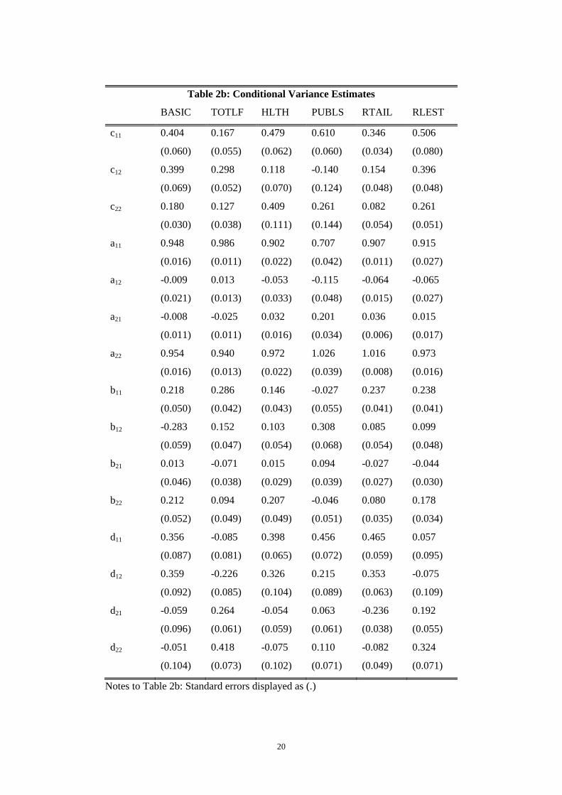
displayed in Tables 2a, 2b and the upper panel of Table 2c.

Shocks to volatility appear highly persistent. Estimates of the main diagonal elements

of *

11A are, in general, close to unity. There is strong evidence of own variance, cross variance

and covariance asymmetry in the data. This is highlighted by the significance of the

parameters in the *

11D matrix. The insignificance of the off-diagonal elements in the *

11B

matrix suggests that the majority of important volatility spillovers from the market to the

sector are associated with negative realisations of ,M tR . Taken together, the evidence

suggests that news about the individual portfolios (market or sector) impacts only upon that

individual portfolio volatility. However, bad news about the market portfolio spills over into

the individual sector portfolios without evidence of feedback from sector to market.

10

The upper panel of Table 2c displays the estimates of the matrix. The conditional

CAPM suggests a positive relationship between the market risk premium and the variance of

the market portfolio. This condition is not supported by the data for the Basic Industries and

Total Financials Sectors with 1,ˆ 0M and significant. Similarly for Total Financials, Retail

and Real Estate 1,ˆ 0SM and significant. As 1,

ˆSM can be interpreted as an estimate of the

coefficient of risk aversion these estimates are not consistent with existing estimates in the

literature, see Hansen and Singleton (1983) inter alia. While the focus of this paper is not on

testing the conditional CAPM, these results are suggestive of the theory being incompatible

with the data.

With the exception of the health sector, the models all pass the usual Ljung-Box test

for serial correlation in the standardised and squared standardised residuals displayed in

Table 2c.

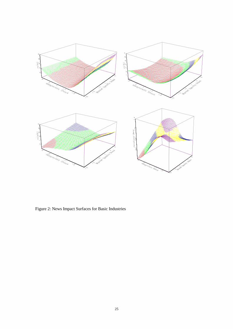
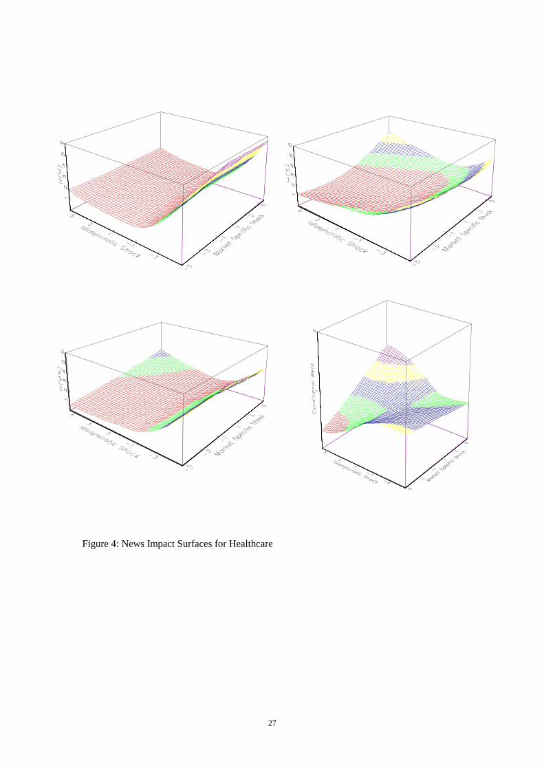
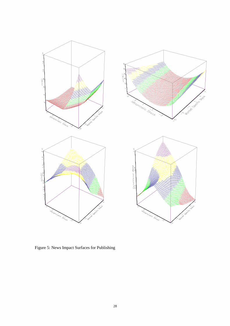
Figures 2-7 display the variance and covariance news impact surfaces for the

estimates of the Multivariate GARCH model displayed in Table 2. Following Engle and Ng

(1993) and Ng and Kroner (1996), each surface is evaluated in the region , 5,5i t for i

= M, S, holding information at time t-1 and before constant. There are relatively few extreme

outliers in the data, which suggests that some caution should be exercised in interpreting the

news impact surfaces for large absolute values of ,i t . Despite this caveat, the asymmetry in

variance and covariance is clear from each Figure. The sign and magnitude of idiosyncratic

and market shocks have clearly differing impacts on elements of tH . The first panel of each

Figure shows the effect of idiosyncratic and market-wide shocks on subsequent market

volatility. It is evident that for the basic industries, healthcare and publishing sectors, positive

idiosyncratic shocks have virtually no effect on next period market volatility, while negative

shocks have moderate impacts. On the other hand, in the cases of the financial and real estate

sectors, idiosyncratic shocks have a much stronger role to play. In the cases of the basic

industries, retail and healthcare sectors, a market-wide shock has a bigger impact on

11

subsequent sector volatility than an idiosyncratic shock of the same size. The third panels of

Figures 2 to 7 show the effects of idiosyncratic and market-wide shocks on future conditional

covariance between market and sector returns. For the basic industries, financial, healthcare

and retail sectors, it appears to be the sector-specific shocks that drive the covariances, with

negative shocks having considerably larger effects than positive shocks of the same

magnitude.

Holding information at time t-1 and before constant, and evaluating ,S t as before

yields the response of the measure of undiversifiable risk to news. The fourth panels of

Figures 2-7 graph the response of ,S t to news using the estimates displayed in Table 2.

Again, the asymmetry in response to market and idiosyncratic shocks is clear. For example,

visual inspection of the fourth panel of Figure 2 suggests the differing response of ,S t to

idiosyncratic and market-wide shocks. The basic industries beta appears to respond largely to

idiosyncratic shocks. On the other hand, Figure 3 suggests that the total financials beta

responds far more to market-wide shocks. In the course of daily business, providing liquidity

and capital, the financial sector becomes exposed to risk across all sectors of the economy;

thus it is intuitively appealing that the beta for the financial sector appears to respond

strongly to news about the market. Such visual analysis, while intuitively appealing, is

obviously ad-hoc and subjective, therefore the paper now moves to a more formal statistical

analysis of the sources of the observed asymmetry.

4. Properties of the ,ˆ

S t series

By construction, the model allows S, the measure of undiversifiable risk associated

with industry sector S to respond asymmetrically to news about the market portfolio and/or

news about sector S. Brooks, Henry and Persand (2002) argue that the dependence of beta on

news is important in the context of dynamic hedging, particularly in the presence of

asymmetries. The third column of Figure 1 plots the estimated ,ˆ

S t . The time variation of the

12

measure of undiversifiable risk across each sector is evident. Table 3 presents descriptive

statistics for the ,ˆ

S t series. The most volatile of the ,ˆ

S t series is associated with the real

estate sector. Here the ,ˆ

S t ranges from a minimum of 0.44 to a maximum of 1.48. In terms of

the average value of ,ˆ

S t , retailing appears to be the riskiest sector, with a ,ˆ

S t =1.11,

indicating that retailing has higher risk than the market portfolio which has , 1M t t by

definition. The averages of the ,ˆ

S t series compare closely with the static estimates presented

in Table 1. On the basis of a sequence of augmented Dickey-Fuller unit root tests, the ,ˆ

S t

series appear stationary.

What factors underlay the observed asymmetry in ,ˆ

S t ? EC argue that shocks to the

market and idiosyncratic shocks determine asymmetric effects in ,ˆ

S t . This logic underlies

the News Impact Surface that we propose for ,ˆ

S t depicted in Figures 2 to 6. To identify

negative returns to the market, let ,M tI represent an indicator variable, which takes the value

of unity when ,M tR , the return to the market portfolio, is negative and zero otherwise.

Similarly, in order to identify the magnitude of negative market returns, let

, , ,M t M t M tR I R . Similar variables may be defined to identify negative return innovations

and the corresponding magnitudes for each individual sector.

Consider the OLS regression

, 1 2 , 3 , 4 , 5 , 6 , ,ˆ

7S t M t M t S t S t S t M t tI R I R C C u (14)

where , , ,S t M t S tC I R , and , , ,M t S t M tC I R represent dummy variables designed to

capture the sector return when the market return is negative ( ,S tC ) and the market return

when the sector return is negative ( ,M tC ).

13

The results from estimation of (14) are displayed in Table 4. Periods of negative

returns to the market only significantly affect ,ˆ

S t for the health sector, leading to a fall in

the value of the measure of undiversifiable risk. However, large negative innovations to the

market portfolio uniformly lead to a significant increase in ,ˆ

S t across all sectors considered.

There is no pattern of correlation between a negative return to the sector and changes in

,ˆ

S t with the sign and significance of 5 being apparently random across sectors. Similarly,

,S tC and ,M tC do not appear to significantly affect estimates of systematic risk.

On the basis of the static estimates of S, the healthcare sector appears least risky.

Using the mean of ,ˆ

S t as a measure of the relative riskiness of the sectors also suggests that

the Healthcare sector is the least risky. However such a ranking clearly ignores relative

uncertainty about the estimates of ,ˆ

S t .

Figure 8 displays the empirical cumulative density functions (CDF) for the six

estimated ,ˆ

S t series. Following González-Rivera (1996), we compare the market risk of the

six sectors using the concepts of stochastic dominance. Here the least risky sector will

dominate. Let XF and YG be the CDF of for sectors X and Y, respectively. If

XF YG for all then X dominates Y in the first order sense. The CDFs are

constructed from the 1, 10, 25, 50, 75, 90, 95 and 99 percentiles. In this context, there is no

first order dominance as the CDFs all cut each other. That is, there is no clear least risky

sector on the first order basis. Second order dominance requires that

0X YF G d

for all . In this context there are 15 possible pairs of series,

so graphical representation is not useful. Using second order dominance, no clear ordering is

obtained. It is therefore not possible to identify a clearly least risky sector using a pair wise

approach. Further investigation of this issue is beyond the scope of the current paper.

14

5. Summary and Conclusions

Recent research provides conflicting evidence as to whether abnormalities in equity

returns are a result of changes in expected returns in an efficient market or an over-reaction to

new information in a market that is inefficient. De Bondt and Thaler (1985), Chopra,

Lakonishok and Ritter (1992), and Jegadeesh and Titman (1993) inter alia, conclude that the

return to a portfolio formed by buying stocks which have suffered capital losses (losers) in

the past, and selling stocks which have experienced capital gains (winners) in the past, has a

higher average return that predicted by the CAPM. All three studies conclude that such over-

reaction is inconsistent with efficiency, since such contrarian strategies should not

consistently earn excess returns.

On the other hand, Chan (1988), and Ball and Kothari (1989) argue that the time

variation in expected return due to time-variation in beta explains the success of the ‘losers’

portfolio. The studies find that there exists predictive asymmetry in the response of the

conditional beta to large positive and negative innovations. Braun, Nelson and Sunier (1995)

find weak evidence of asymmetry in beta, but conclude that it is not sufficient to explain the

over-reaction to information, or mean reversion in stock prices. Engle and Cho (1999) argue

that this lack of evidence of asymmetry in beta is due to stock price aggregation, and lack of

cross-sectional variation in the monthly data used by Braun, Nelson and Sunier (1995). Engle

and Cho (1999) suggest that the use of daily data on individual stocks makes the detection of

asymmetry an easier task.

This paper employs weekly data on industry sectors from the UK equity market to

examine the impact of news on time-varying measures of beta. The use of weekly data on

sectors of the market should overcome the potential price aggregation problems associated

with lower frequency data, and maintain sufficient cross-sectional variation to detect time

variation and asymmetry in beta.

Treating logarithmic price innovations as a collective measure of news arriving to the

market between time t –1 and time t, the results suggest that time-variation in beta depends

15

on two sources of news - news about the market and news about the sector. However, the

asymmetric response of beta to news appears related only to large negative innovations to the

market. Bad news about each individual sector does not appear to significantly affect the

measure of undiversifiable risk. The asymmetric effect in beta is consistent across all sectors

considered.

Given the magnitude of the asymmetry identified in beta, the evidence in this paper

suggests that abnormalities such as mean reversion in stock prices may occur as a result of

changes in expected return caused by time-variation and asymmetry in beta, rather than as a

by-product of market inefficiency.

There is some evidence that the healthcare industry is the least risky of the sectors

considered. However this evidence is at best indicative and does not take into account the

higher moments of the empirical distribution of the estimated measures of market risk.

Taking uncertainty about ,ˆ

S t into account it is not possible to order the sectors in terms of

exposure to market risk. Further research on this subject is clearly a matter of interest.

16

References Akaike, H., (1974) “New look at statistical model identification”, I.E.E.E Transactions on

Automatic Control, AC-19, 716-723.

Attanasio, O.P. (1991) “Risk, time varying second moments and market efficiency”, Review

of Economic Studies, 58, 479-494.

Baillie, R.T. and Myers, R.J. (1991) “Bivariate GARCH Estimation of the Optimal

Commodity Futures Hedge” Journal of Applied Econometrics, 6, 109-124.

Ball, R., and Kothari, S.P. (1989) “Non-stationary expected returns: Implications for tests of

market efficiency and serial correlation in returns”, Journal of Financial Economics, 25, 51-

74.

Black, F. (1976) “Studies in price volatility changes”, Proceedings of the 1976 Meeting of the

Business and Economics Statistics Section, American Statistical Association, 177-181.

Bollerslev, T., Engle, R.F. and Wooldridge, J.M. (1988) “A capital asset pricing model with

time-varying covariances”, Journal of Political Economy, 96, 116-31.

Braun, P.A., Nelson, D.B., and Sunier, A.M. (1995) “Good News, Bad News, Volatility and

Betas”, Journal of Finance, 50, 1575-1603.

Brooks C. and Henry, Ó. T. (2000), “Linear and Non-Linear Transmission of Equity Return

Volatility: Evidence from the US, Japan and Australia”, Economic Modelling, 17, 497-513.

Brooks, C., Henry Ó.T. and Persand, G. (2002) “The Effect of Asymmetries on Optimal

Hedge Ratios” Journal of Business 75(2), 333-352.

Campbell, J. and Hentschel, L. (1992) “No news is good news: An asymmetric model of

changing volatility in stock returns”, Journal of Financial Economics, 31, 281-318.

Christie, A. (1982) “The stochastic behaviour of common stock variance: Value, leverage and

interest rate effects”, Journal of Financial Economics, 10, 407-432.

Chopra, N., Lakonishok, J., and Ritter, J. (1992) “Measuring abnormal returns: Do stocks

overreact?” Journal of Financial Economics, 10, 289-321.

DeBondt, W., and Thaler, R., (1985) “Does the stock market overreact?” The Journal of

Finance, 40, 793-805

Engel, C., Frankel, J.A., Froot, K.A., and Rodrigues, A.P. (1995) “Tests of Conditional

Mean-Variance Efficiency of the U.S. Stock Market”, Journal of Empirical Finance, 2, 3-18.

Engle, R.F. (1982) “Autoregressive conditional heteroscedasticity with estimates of the

variance of United Kingdom inflation”, Econometrica, 50, 987-1007.

Engle, R.F., and Cho, Y-H, (1999) “Time Varying Betas and Asymmetric Effects of News:

Empirical Analysis of Blue Chip Stocks”, NBER Working Paper No 7330

Engle, R.F and Kroner, K. (1995) “Multivariate simultaneous generalized ARCH”,

Econometric Theory, 11, 122-150.

17

Engle, R.F. and Ng, V. (1993) “Measuring and testing the impact of news on volatility”,

Journal of Finance, 48, 1749-1778.

Glosten, L.R., Jagannathan, R. and Runkle, D. (1993) “On the relation between the expected

value and the volatility of the nominal excess return on stocks”, Journal of Finance, 48,

1779-1801.

González-Rivera, G. (1996) “Time varying risk: The case of the American computer

industry”, Journal of Empirical Finance, 2, 333-342.

Hansen L.P. and Singleton, K. (1983) “Stochastic consumption, risk aversion, and the

temporal behaviour of asset returns”, Journal of Political Economy, 91, 249-266.

Henry, Ó.T. (1998) “Modelling the Asymmetry of Stock Market Volatility”, Applied

Financial Economics, 8, 145 - 153.

Henry, Ó.T. and Sharma J.S. (1999) “Asymmetric Conditional Volatility and Firm Size:

Evidence from Australian Equity Portfolios”, Australian Economic Papers, 38, 393 – 407

Jegadeesh, N., and Titman, S., (1993) “Returns to buying winners and selling losers:

Implications for stock market efficiency”, Journal of Finance, 48, 65-91.

Kroner, K.F. and Sultan, J. (1991) “Exchange Rate Volatility and Time Varying Hedge

Ratios” in Rhee, S.G. and Chang, R.P. (eds.) Pacific Basin Capital Markets Research

Elsevier, North Holland

Kroner, K.F., and Ng, V.K. (1996) “Multivariate GARCH Modelling of Asset Returns”,

Papers and Proceedings of the American Statistical Association, Business and Economics

Section, 31-46.

Merton, R.C. (1973) “An Intertemporal Asset Pricing Model”, Econometrica, 41, 867-887.

Merton, R.C. (1980) “On Estimating the Expected Return on the Market: An Exploratory

Investigation”, Journal of Financial Economics, 8, 323-361.

Pagan, A.R., and Schwert, G.W. (1990) “Alternative Models for Conditional Stock

Volatility”, Journal of Econometrics, 45, 267-290

Schwarz, G. (1978) “Estimating the dimensions of a model”, Annals of Statistics, 6, 461-464.

18

Tables and Figures

Table 1: Summary statistics for the returns data

Series Mean Variance Skew E.K. 1 Q(5) Q2(5)

FTALL 0.280 6.288 -0.323

[0.000]

9.082

[0.000]

0.071 56.67

[0.000]

231.036

[0.000]

1.00

BASIC 0.226 7.690 -0.517

[0.000]

7.975

[0.000]

0.079 44.447

[0.000]

55.825

[0.000]

0.976

(0.012)

TOTLF 0.303 7.260 0.007

[0.900]

6.941

[0.000]

0.111 56.668

[0.000]

342.389

[0.000]

0.978

(0.010)

HLTH 0.280 10.842 -0.061

[0.290]

5.459

[0.000]

0.016 21.715

[0.001]

155.245

[0.000]

0.930

(0.022)

PUBLS 0.245 9.883 -0.650

[0.000]

10.531

[0.000]

0.107 48.013

[0.000]

107.912

[0.000]

1.040

(0.016)

RTAIL 0.256 11.129 0.168

[0.000]

3.737

[0.000]

0.002 6.009

[0.305]

122.797

[0.000]

1.079

(0.018)

RLEST 0.249 11.908 -0.159

[0.000]

6.579

[0.000]

0.097 33.713

[0.000]

391.338

[0.000]

1.032

(0.021)

Notes to Table 1: Marginal significance levels displayed as [.], standard errors displayed as

(.). Skew measures the standardised third moment of the distribution and reports the marginal

significance of a test for zero skewness. E.K. reports the excess kurtosis of the return

distribution and the associated marginal significance level for the test of zero excess kurtosis.

The first order autocorrelation coefficient is 1. Q(5) and Q2(5) are Ljung-Box tests for fifth

order serial correlation in the returns and the squared returns, respectively. Both tests are

distributed as 2(5) under the null. is the OLS estimate of the measure of undiversifiable

risk.

19

Table 2a: Conditional Mean Estimates

BASIC TOTLF HLTH PUBLS RTAIL RLEST

)(M 0.336

(0.043)

0.288

(0.053)

0.157

(0.041)

0.207

(0.0350)

0.099

(0.034)

0.258

(0.038)

)(

,1

M

M -0.171

(0.017)

-0.033

(0.011)

0.199

(0.028)

-0.086

(0.018)

0.171

(0.012)

-0.103

(0.019)

)(

,2

M

M 0.130

(0.011)

0.055

(0.010)

0.038

(0.015)

0.114

(0.015)

0.145

(0.012)

0.087

(0.013)

)(

,1

M

S 0.051

(0.009)

0.042

(0.011)

0.002

(0.012)

0.047

(0.021)

0.036

(0.009)

0.018

(0.011)

)(

,2

M

S -0.003

(0.011)

0.062

(0.008)

0.062

(0.011)

0.005

(0.011)

-0.024

(0.009)

0.026

(0.010)

)(

,1

M

M 0.153

(0.016)

0.008

(0.012)

-0.019

(0.024)

0.061

(0.021)

-0.202

(0.012)

0.117

(0.020)

)(S 0.150

(0.013)

0.363

(0.068)

0.134

(0.068)

0.242

(0.038)

0.222

(0.057)

0.160

(0.045)

)(

,1

S

M -0.023

(0.013)

0.005

(0.012)

0.117

(0.021)

0.053

(0.030)

-0.021

(0.021)

0.003

(0.018)

)(

,2

S

M 0.113

(0.018)

0.032

(0.011)

0.090

(0.020)

0.216

(0.017)

0.156

(0.020)

0.040

(0.018)

)(

,1

S

S 0.147

(0.019)

-0.011

(0.010)

-0.097

(0.015)

0.056

(0.016)

-0.057

(0.013)

0.094

(0.012)

)(

,2

S

S 0.002

(0.012)

0.080

(0.010)

0.008

(0.015)

-0.048

(0.013)

-0.071

(0.013)

0.009

(0.012)

)(

,1

S

S -0.089

(0.021)

0.062

(0.011)

0.053

(0.014)

-0.016

(0.021)

0.031

(0.013)

-0.003

(0.013)

Notes to Table 2a: Standard errors displayed as (.)

20

Table 2b: Conditional Variance Estimates

BASIC TOTLF HLTH PUBLS RTAIL RLEST

c11 0.404

(0.060)

0.167

(0.055)

0.479

(0.062)

0.610

(0.060)

0.346

(0.034)

0.506

(0.080)

c12 0.399

(0.069)

0.298

(0.052)

0.118

(0.070)

-0.140

(0.124)

0.154

(0.048)

0.396

(0.048)

c22 0.180

(0.030)

0.127

(0.038)

0.409

(0.111)

0.261

(0.144)

0.082

(0.054)

0.261

(0.051)

a11 0.948

(0.016)

0.986

(0.011)

0.902

(0.022)

0.707

(0.042)

0.907

(0.011)

0.915

(0.027)

a12 -0.009

(0.021)

0.013

(0.013)

-0.053

(0.033)

-0.115

(0.048)

-0.064

(0.015)

-0.065

(0.027)

a21 -0.008

(0.011)

-0.025

(0.011)

0.032

(0.016)

0.201

(0.034)

0.036

(0.006)

0.015

(0.017)

a22 0.954

(0.016)

0.940

(0.013)

0.972

(0.022)

1.026

(0.039)

1.016

(0.008)

0.973

(0.016)

b11 0.218

(0.050)

0.286

(0.042)

0.146

(0.043)

-0.027

(0.055)

0.237

(0.041)

0.238

(0.041)

b12 -0.283

(0.059)

0.152

(0.047)

0.103

(0.054)

0.308

(0.068)

0.085

(0.054)

0.099

(0.048)

b21 0.013

(0.046)

-0.071

(0.038)

0.015

(0.029)

0.094

(0.039)

-0.027

(0.027)

-0.044

(0.030)

b22 0.212

(0.052)

0.094

(0.049)

0.207

(0.049)

-0.046

(0.051)

0.080

(0.035)

0.178

(0.034)

d11 0.356

(0.087)

-0.085

(0.081)

0.398

(0.065)

0.456

(0.072)

0.465

(0.059)

0.057

(0.095)

d12 0.359

(0.092)

-0.226

(0.085)

0.326

(0.104)

0.215

(0.089)

0.353

(0.063)

-0.075

(0.109)

d21 -0.059

(0.096)

0.264

(0.061)

-0.054

(0.059)

0.063

(0.061)

-0.236

(0.038)

0.192

(0.055)

d22 -0.051

(0.104)

0.418

(0.073)

-0.075

(0.102)

0.110

(0.071)

-0.082

(0.049)

0.324

(0.071)

Notes to Table 2b: Standard errors displayed as (.)

21

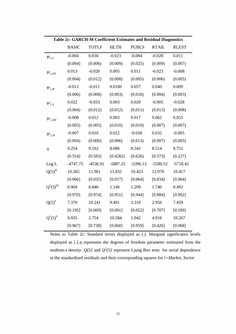
Table 2c: GARCH-M Coefficient Estimates and Residual Diagnostics

BASIC TOTLF HLTH PUBLS RTAIL RLEST

1,S -0.004

(0.004)

0.030

(0.006)

-0.023

(0.009)

-0.084

(0.025)

-0.028

(0.009)

0.011

(0.007)

1,SM 0.013

(0.004)

-0.020

(0.012)

0.005

(0.008)

0.011

(0.005)

-0.023

(0.006)

-0.008

(0.005)

1,M -0.011

(0.006)

-0.011

(0.008)

0.0180

(0.003)

0.057

(0.018)

0.040

(0.004)

0.009

(0.003)

2,S 0.022

(0.004)

-0.033

(0.012)

0.003

(0.012)

0.020

(0.011)

-0.005

(0.013)

-0.028

(0.008)

2,SM -0.008

(0.005)

0.012

(0.005)

0.003

(0.010)

0.017

(0.010)

0.062

(0.007)

0.055

(0.007)

2,M -0.007

(0.004)

0.010

(0.006)

0.012

(0.006)

-0.028

(0.013)

0.032

(0.007)

-0.005

(0.005)

9.254

(0.554)

9.162

(0.583)

8.086

(0.4282)

8.345

(0.626)

8.514

(0.573)

8.751

(0.227)

Log L -4747.75 -4536.92 -5887.25 -5396.13 -5580.52 -5718.42

Q(5)M

10.365

[0.066]

11.961

[0.035]

13.832

[0.017]

10.423

[0.064]

12.070

[0.034]

10.417

[0.064]

Q2(5)

M 0.904

[0.970]

0.846

[0.974]

1.140

[0.951]

1.209

[0.944]

1.740

[0.884]

0.492

[0.992]

Q(5)S 7.370

[0.195]

10.241

[0.069]

9.491

[0.091]

3.310

[0.652]

2.956

[0.707]

7.459

[0.189]

Q2(5)

S 0.935

[0.967]

2.754

[0.738]

10.584

[0.060]

1.042

[0.959]

4.916

[0.426]

10.267

[0.068]

Notes to Table 2c: Standard errors displayed as (.). Marginal significance levels

displayed as [.]. represents the degrees of freedom parameter estimated from the

students-t density. Q(5)i and Q

2(5)

i represent Ljung Box tests for serial dependence

in the standardised residuals and their corresponding squares for i=Market, Sector

22

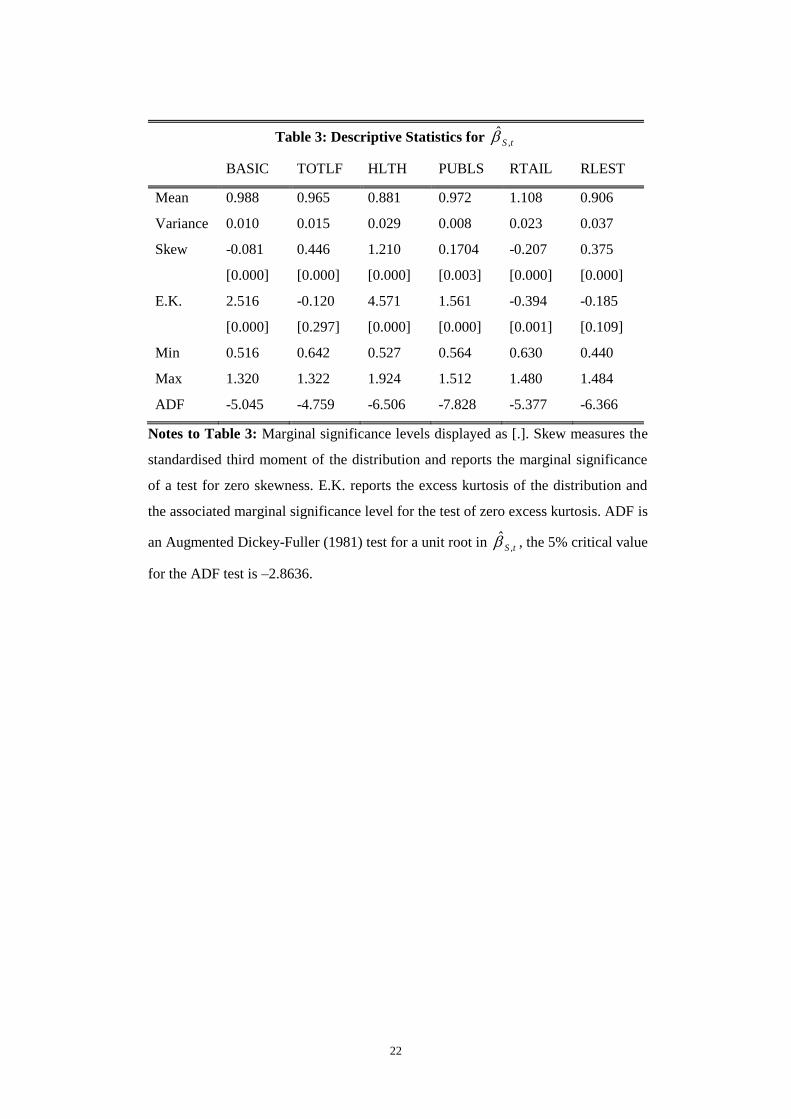
Table 3: Descriptive Statistics for tS ,̂

BASIC TOTLF HLTH PUBLS RTAIL RLEST

Mean 0.988 0.965 0.881 0.972 1.108 0.906

Variance 0.010 0.015 0.029 0.008 0.023 0.037

Skew -0.081

[0.000]

0.446

[0.000]

1.210

[0.000]

0.1704

[0.003]

-0.207

[0.000]

0.375

[0.000]

E.K. 2.516

[0.000]

-0.120

[0.297]

4.571

[0.000]

1.561

[0.000]

-0.394

[0.001]

-0.185

[0.109]

Min 0.516 0.642 0.527 0.564 0.630 0.440

Max 1.320 1.322 1.924 1.512 1.480 1.484

ADF -5.045 -4.759 -6.506 -7.828 -5.377 -6.366

Notes to Table 3: Marginal significance levels displayed as [.]. Skew measures the

standardised third moment of the distribution and reports the marginal significance

of a test for zero skewness. E.K. reports the excess kurtosis of the distribution and

the associated marginal significance level for the test of zero excess kurtosis. ADF is

an Augmented Dickey-Fuller (1981) test for a unit root in tS ,̂ , the 5% critical value

for the ADF test is –2.8636.

23

Table 4: Sources of Asymmetry in tS ,̂

BASIC TOTLF HLTH PUBLS RTAIL RLEST

1 0.993*

(0.003)

0.959*

(0.004)

0.900*

(0.006)

0.983*

(0.003)

1.237*

(0.005)

0.909*

(0.006)

2 0.008

(0.007)

0.004

(0.009)

-0.040*

(0.011)

-0.007

(0.006)

0.002

(0.010)

-0.011

(0.012)

3 0.056*

(0.007)

0.052*

(0.012)

0.019*

(0.008)

0.040*

(0.005)

0.051*

(0.009)

0.027*

(0.009)

4 -0.001

(0.007)

-0.009

(0.009)

-0.039*

(0.011)

-0.015*

(0.006)

-0.007

(0.011)

-0.065*

(0.011)

5 0.023*

(0.007)

-0.032*

(0.010)

-0.019*

(0.005)

-0.001

(0.005)

-0.009

(0.006)

-0.035*

(0.006)

6 -0.036*

(0.006)

-0.012

(0.012)

-0.014

(0.008)

-0.022

(0.005)

-0.027*

(0.009)

-0.016*

(0.008)

7 -0.039*

(0.007)

-0.017

(0.010)

-0.004

(0.005)

-0.020*

(0.004)

-0.022*

(0.006)

-0.014*

(0.006)

LM 135.120

[0.000]

141.991

[0.000]

88.279

[0.000]

173.451

[0.000]

78.217

[0.000]

285.049

[0.000]

Notes to Table 4: Marginal significance levels displayed as [.]. Standard errors

displayed as (.). * denotes significance at the 5% level.

24

B a s i c I n d u s t r i e s I n d e x

1 9 6 51 9 6 81 9 7 11 9 7 41 9 7 71 9 8 01 9 8 31 9 8 61 9 8 91 9 9 21 9 9 51 9 9 80

1 0 0 0

2 0 0 0

3 0 0 0

4 0 0 0

5 0 0 0

6 0 0 0

7 0 0 0

T o t a l F i n a n c i a l s I n d e x

1 9 6 51 9 6 81 9 7 11 9 7 41 9 7 71 9 8 01 9 8 31 9 8 61 9 8 91 9 9 21 9 9 51 9 9 80

5 0 0 0

1 0 0 0 0

1 5 0 0 0

2 0 0 0 0

2 5 0 0 0

3 0 0 0 0

H e a l t h C a r e I n d e x

1 9 6 51 9 6 81 9 7 11 9 7 41 9 7 71 9 8 01 9 8 31 9 8 61 9 8 91 9 9 21 9 9 51 9 9 8

0

2 5 0 0

5 0 0 0

7 5 0 0

1 0 0 0 0

1 2 5 0 0

1 5 0 0 0

1 7 5 0 0

P u b l i s h i n g I n d e x

1 9 6 51 9 6 81 9 7 11 9 7 41 9 7 71 9 8 01 9 8 31 9 8 61 9 8 91 9 9 21 9 9 51 9 9 80

1 0 0 0

2 0 0 0

3 0 0 0

4 0 0 0

5 0 0 0

6 0 0 0

7 0 0 0

8 0 0 0

9 0 0 0

R e t a i l I n d e x

1 9 6 51 9 6 81 9 7 11 9 7 41 9 7 71 9 8 01 9 8 31 9 8 61 9 8 91 9 9 21 9 9 51 9 9 8

0

2 0 0 0

4 0 0 0

6 0 0 0

8 0 0 0

1 0 0 0 0

1 2 0 0 0

1 4 0 0 0

1 6 0 0 0

R e a l E s t a t e I n d e x

1 9 6 51 9 6 81 9 7 11 9 7 41 9 7 71 9 8 01 9 8 31 9 8 61 9 8 91 9 9 21 9 9 51 9 9 80

2 0 0 0

4 0 0 0

6 0 0 0

8 0 0 0

1 0 0 0 0

1 2 0 0 0

B a s i c I n d u s t r i e s R e t u r n

1 9 6 51 9 6 81 9 7 11 9 7 41 9 7 71 9 8 01 9 8 31 9 8 61 9 8 91 9 9 21 9 9 51 9 9 8- 3 0

- 2 5

- 2 0

- 1 5

- 1 0

- 5

0

5

1 0

1 5

T o t a l F i n a n c i a l s R e t u r n

1 9 6 51 9 6 81 9 7 11 9 7 41 9 7 71 9 8 01 9 8 31 9 8 61 9 8 91 9 9 21 9 9 51 9 9 8- 2 4

- 1 6

- 8

0

8

1 6

2 4

H e a l t h C a r e R e t u r n

1 9 6 51 9 6 81 9 7 11 9 7 41 9 7 71 9 8 01 9 8 31 9 8 61 9 8 91 9 9 21 9 9 51 9 9 8

- 3 0

- 2 0

- 1 0

0

1 0

2 0

3 0

P u b l i s h i n g R e t u r n

1 9 6 51 9 6 81 9 7 11 9 7 41 9 7 71 9 8 01 9 8 31 9 8 61 9 8 91 9 9 21 9 9 51 9 9 8- 3 6

- 2 4

- 1 2

0

1 2

2 4

R e t a i l R e t u r n

1 9 6 51 9 6 81 9 7 11 9 7 41 9 7 71 9 8 01 9 8 31 9 8 61 9 8 91 9 9 21 9 9 51 9 9 8

- 2 4

- 1 6

- 8

0

8

1 6

2 4

R e a l E s t a t e R e t u r n

1 9 6 51 9 6 81 9 7 11 9 7 41 9 7 71 9 8 01 9 8 31 9 8 61 9 8 91 9 9 21 9 9 51 9 9 8- 2 4

- 1 6

- 8

0

8

1 6

2 4

3 2

B a s i c I n d u s t r i e s B e t a

1 9 6 51 9 6 81 9 7 11 9 7 41 9 7 71 9 8 01 9 8 31 9 8 61 9 8 91 9 9 21 9 9 51 9 9 80 . 5

0 . 6

0 . 7

0 . 8

0 . 9

1 . 0

1 . 1

1 . 2

1 . 3

1 . 4

T o t a l F i n a n c i a l s B e t a

1 9 6 51 9 6 81 9 7 11 9 7 41 9 7 71 9 8 01 9 8 31 9 8 61 9 8 91 9 9 21 9 9 51 9 9 80 . 6

0 . 7

0 . 8

0 . 9

1 . 0

1 . 1

1 . 2

1 . 3

1 . 4

H e a l t h C a r e B e t a

1 9 6 51 9 6 81 9 7 11 9 7 41 9 7 71 9 8 01 9 8 31 9 8 61 9 8 91 9 9 21 9 9 51 9 9 8

0 . 5 0

0 . 7 5

1 . 0 0

1 . 2 5

1 . 5 0

1 . 7 5

2 . 0 0

P u b l i s h i n g B e t a

1 9 6 51 9 6 81 9 7 11 9 7 41 9 7 71 9 8 01 9 8 31 9 8 61 9 8 91 9 9 21 9 9 51 9 9 80 . 5 6

0 . 7 0

0 . 8 4

0 . 9 8

1 . 1 2

1 . 2 6

1 . 4 0

1 . 5 4

R e t a i l B e t a

1 9 6 51 9 6 81 9 7 11 9 7 41 9 7 71 9 8 01 9 8 31 9 8 61 9 8 91 9 9 21 9 9 51 9 9 8

0 . 6

0 . 7

0 . 8

0 . 9

1 . 0

1 . 1

1 . 2

1 . 3

1 . 4

1 . 5

R e a l E s t a t e B e t a

1 9 6 51 9 6 81 9 7 11 9 7 41 9 7 71 9 8 01 9 8 31 9 8 61 9 8 91 9 9 21 9 9 51 9 9 80 . 4

0 . 6

0 . 8

1 . 0

1 . 2

1 . 4

1 . 6

Figure 1: Sector index, sector return and estimated sector beta

25

Figure 2: News Impact Surfaces for Basic Industries

26

Figure 3: News Impact Surfaces for Total Financial

27

Figure 4: News Impact Surfaces for Healthcare

28

Figure 5: News Impact Surfaces for Publishing

29

Figure 6: News Impact Surfaces for Retail

30

Figure 7: News Impact Surfaces for Real Estate

31

C D B A S I C B

C D T O T L F B

C D H L T H C B

C D P U B L S B

C D R L E S T B

C D R T A I L B

B e t a

0 . 2 50 . 5 00 . 7 51 . 0 01 . 2 51 . 5 01 . 7 52 . 0 0

0 . 0 0

0 . 2 5

0 . 5 0

0 . 7 5

1 . 0 0

Figure 8: Cumulative distribution functions for the Sector ,ˆ

S t