The impact of HIV/AIDS on household economy in two

villages in Salima district, MalawiJohn Seaman and Celia Petty, with James Acidri

DRAFT COPY - FEBRUARY 2005

Funded by Save the Children UK

2

Field Research Team: James Acridri , Gabriela Chapota, Hellen Fatchi,Richard Kajombo, Leonard Mushani, Stanley Mvula, , Celia Petty, JohnSeaman, Condwani Zimba (facilitator and field researcher)Moussa Mafuta (translator)

Acknowledgements

We are very grateful to the staff of Save the Children US and to Save theChildren UK for their support in implementing this survey and communitymembers in the two study sites who helped in our work.

3

HIV/AIDS and Household Economy in Two Villages in Salimadistrict, Malawi

A Study conducted in September 20041. Introduction

This is the third in a series of studies undertaken in southern Africa, with the aim of

improving understanding of the relationship between HIV/AIDS, poverty and food

security 1. The earlier studies were carried out in Swaziland and Mozambique in

2003. In one of these studies, Swaziland, an attempt was made to estimate the

impact of HIV/AIDS on individual household economies. It was found that although

the impact was negative, and for some households catastrophic, the average size of

the impact was comparatively small relative to the effect of other economic

fluctuations, chiefly because many of the people affected were under employed or

unemployed. It was also found that many of the commonly used indicators of

HIV/AIDS vulnerability (for example, the presence of orphans in the household,

chronic illness, the proportion of available land cultivated etc) provided a poor guide

to a more objective estimate of need. However, both the Swaziland and Mozambique

studies were located in countries and communities that were, by the standards of

rural southern Africa, comparatively affluent. The Malawi study was carried out in

Salima district, which has a recent history of famine2, high levels of poverty and a

lack of off farm employment options, as well as a high prevalence of HIV/AIDS. 3

The aim of this study was to inform the wider debate around effective programming

for orphans and vulnerable children (OVCs) by

� exploring whether there were differences in the relationship between orphans,

poverty and food security in a poorer setting than the two earlier studies.

1 HIV/AIDS and household economy in a Highveld Swaziland community (Seaman J, Petty Cwith Narangui H. SC UK March 2004) A rural trading community in Manica province,Mozambique: the impact of HIV/AIDS on household economy (Petty C, Sylvester K, SeamanJ. SC UK March 2004)2 Distress migration from rural areas to Salima town occurred in 2002; there were choleradeaths among the displaced and malnutrition rates of 19% were recorded3 HIV prevalence rates in Salima range from 13%-25% (Salima Socio-economic profileRepublic of Malawi 2002) . HIV prevalence in the Swaziland site was 38% and theMozambique site was around 21%

4

� demonstrating a practical methodology for field research and data analysis that

provides reliable, quantitative descriptions of household economy and

demography in extremely poor, HIV affected communities.

� modelling a range of interventions and their impact on poor households (including

households with and without orphans).

This report presents a summary of the main findings of the study. A number of

issues, including the choice of interventions to more effectively reduce levels of

poverty and vulnerability and the implications of different targeting methods, will be

treated in greater depth, and comparisons made with the findings of the other two

studies, in a future paper.

2. Background and context: Salima district4

Salima district is located in the central region of Malawi bordering the western side of

Lake Malawi.. The district extends from the Rift Valley lakeshore plain (altitude 200m-

500 m) adjacent to Lake Malawi, to the central upland area in the west (altitude 500m

-1000 m).

Salima has one main rainy season (November to April) and average temperatures of

around 22 C. Lowland soils are made up of clay loam and alluvial deposits and

include extensive dambos 5. The upland areas have shallow stony soils.

Salima has one of the highest rates of soil erosion in the country, with a registered

soil loss of 41-50 ha/year. There has been extensive deforestation and the estimated

current rate of deforestation across the district is just under 4%.6

Customary land comprises 76% of the district and can be allocated by Traditional

Authorities (local chiefs). 20% of land is held privately and is mostly used by estate

farmers for commercial farming. The District has 486 private estates, occupying

56146 ha (average around 115 ha). 4% of land is used for schools, hospitals, forest

reserves and markets.

4 See also Salima socio-economic profile, (Republic of Malawi, 2002)5 Defined as 'seasonally waterlogged, predominantly grass covered depressions borderingheadwater drainage lines'

5

Demography, population characteristics and availability of services

Population

The 1998 Population and Housing Census recorded a district population of 248,214

people. Salima district had an annual population growth rate of 2.5% between

1987/1998. At that time, children aged less than 9 years made up around 33% of the

population.

Education

Primary education is available free of charge. However, around 30% of primary

school children have an average travel time to school of over an hour. Pupils are

expected to provide books, school materials and to pay an annual ‘community

contribution’. Staff: pupil ratios are above the national average and there is a

shortage of staff housing. Literacy rates in Salima are low (around 38%).

Health and health services

Infant mortality is estimated at 132 per 10007. There is one referral hospital in the

district. 42% of the population lives within 2 hours’ walk of a health post and 29% of

the population within 1 hours’ walk. Malaria, anaemia and pneumonia are the main

causes of under 5-year hospitalisation. Estimates of the prevalence of HIV/AIDS

ranges from 25-13%.

Water

Only 43% of the population has access safe drinking water. Charges are made for

access to boreholes and other improved water sources.

Electricity

2% of the population has access to electricity and 80% use paraffin for lighting.

Roads and Transport

Two well-maintained main tarmac roads pass through Salima. Most of the remaining

road infrastructure (around 77%), including feeder roads connecting villages and

rural trading centres, become impassable in the rainy season.8

6 See Salima Socio-economic profile, (Republic of Malawi, 2002)7 National infant mortality is 121 per 10008 Salima socio-economic profile 2002

6

Main sources of income

Crops

More than 75% of land in Salima used for crop production, including maize, pulses,

groundnuts, cotton, tobacco, cassava, sorghum, sweet potatoes, mangoes and

bananas. Rain fed maize is the main crop, occupying 40% of arable land. Cotton and

tobacco are the main cash crops. Tobacco production has fallen in the past 3 years

(from 1,013,656 MT in 1999-2000 T to 997,386 MT in 2001-02). Cotton production

increased in the same period from 5,521 MT to 7,529 MT. It has been suggested that

this is due to lower input costs.

Livestock

Despite good conditions for cattle production, livestock are mainly limited to goats,

pigs and chickens. Lack of cattle is explained by problems of disease, raiding and

widespread poverty, preventing farmers from building up herds or restocking to

replace losses.

Sources of employment

Agricultural labour, mainly on private estates, is the main source of income for an

estimated 85% of the district's population. In lakeshore areas fishing also provides

employment. Other employment opportunities, including government service, NGOs

and private business, are extremely limited

Around 80% of households are engaged in farming.

Food aid and Community Based Organisations (CBO)

From 2003 to June 2004, a special food aid distribution (‘food aid plus’) was made

available to ‘orphans and vulnerable households’. SC UK carried out the distribution

in the study area. Food was made available to local community based organisations

(CBOs) which were responsible for targeting assistance, with the co-operation of

community leaders.9 The monthly ration was made up of 50 kg maize, 25 kg soya, 4

litres cooking oil and 50 kg beans. There are 9 registered orphan care support

programmes in Salima. In addition to their role in food aid distribution these groups

are also involved in implementing a range of HIV/AIDS and OVC programmes.

9 The source of food was WFP stocks from the previous year’s emergency programme

7

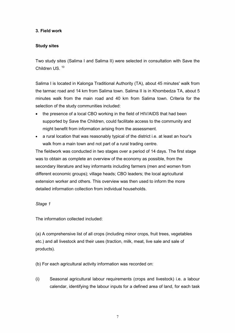
3. Field work

Study sites

Two study sites (Salima I and Salima II) were selected in consultation with Save the

Children US. 10

Salima I is located in Kalonga Traditional Authority (TA), about 45 minutes' walk from

the tarmac road and 14 km from Salima town. Salima II is in Khombedza TA, about 5

minutes walk from the main road and 40 km from Salima town. Criteria for the

selection of the study communities included:

� the presence of a local CBO working in the field of HIV/AIDS that had been

supported by Save the Children, could facilitate access to the community and

might benefit from information arising from the assessment.

� a rural location that was reasonably typical of the district i.e. at least an hour's

walk from a main town and not part of a rural trading centre.

The fieldwork was conducted in two stages over a period of 14 days. The first stage

was to obtain as complete an overview of the economy as possible, from the

secondary literature and key informants including farmers (men and women from

different economic groups); village heads; CBO leaders; the local agricultural

extension worker and others. This overview was then used to inform the more

detailed information collection from individual households.

Stage 1

The information collected included:

(a) A comprehensive list of all crops (including minor crops, fruit trees, vegetables

etc.) and all livestock and their uses (traction, milk, meat, live sale and sale of

products).

(b) For each agricultural activity information was recorded on:

(i) Seasonal agricultural labour requirements (crops and livestock) i.e. a labour

calendar, identifying the labour inputs for a defined area of land, for each task

8

(e.g. land preparation), and who (men/women/children) typically does this

work.

(ii) The costs of all crop and livestock inputs (land, labour, fertilisers and

pesticides, veterinary services etc); the yields expected at different input

levels and for upland and dambo cultivation; and details of seasonal prices.

(iii) All types of employment. For each type of paid employment (including

salaried and self-employment) information was obtained on the amount of

labour typically available for each type of employment (days per month),

seasonal variation in this, typical wage rates, and any requirements for

employment (e.g. age, gender, skill or qualifications).

(iv) Market information, including the names and locations of local markets for

goods and services. Information was collected on the operation of markets,

e.g. price setting for major traded commodities and on local barter

arrangements (eg maize for fish).

(v) Information on credit, loans and local farm input support schemes.

(vi) Information on the social and economic context e.g. land tenure and

inheritance, who in the extended family is normally considered responsible for

supporting orphans, the availability of external NGO and government support

etc.

(vii) A map of the community. Each homestead and the name of the household

head was drawn on a sketch map, to assist in the location of households and

to ensure that all households were visited.

Stage 2

The second part of the fieldwork involved individual household interviews.

Two questionnaires were designed and administered separately. 1. A census

questionnaire. 2. An economic questionnaire. The economic questionnaire was 10 SC US supports CBOs implementing programmes for orphans and vulnerable children in

9

designed on the basis of information obtained in the first stage of the enquiry, to

ensure that all potential income sources were included. The census questionnaire

sought information on all people normally resident in the household (i.e people

usually sleeping and eating there) and included details of household members

absent at the time of the census, orphan status, the relationship of each household

member to the head of household, and school attendance of each child. Additional

information on orphans included the year in which their parent or parents died and

the last occupation of the deceased parent. In the case of female-headed

households, women were identified as never married, widowed or divorced.

The economic questionnaire included:

(i) All sources and amounts of household income in the defined reference year,

whether obtained from household production (food and cash crops, livestock

production, wild foods and gifts 11) or in cash or food from paid employment

and self-employment . This chiefly includes agricultural labour (‘Ganyu’) and

trade (i.e. the sale of cash and food crops, livestock and livestock products,

wild foods, cash gifts, handicrafts etc).

(ii) Household assets (livestock, hoes and other agricultural implements, bicycles

etc). Information on cash savings was not sought, as it was not thought that

accurate information would be obtained.

(iii) The use of agricultural inputs in the reference year.

For this assessment, the reference year, was defined as the year preceding the

survey (Oct 2003-September 2004).

In Salima I, all households were included in the census. Because of the large number

of households, a 50% sample was taken for the economic interviews. To avoid

selection bias every second household was selected from the map. In Salima II, a

smaller village, all households were included in both the census and economic

survey.

The assessment team

The team included 5 field assistants (recent graduates in agricultural science); a

translator/facilitator; a team leader with experience of the individual household the study sites

10

method (IHM) and two experts with responsibility for overall design, implementation,

analysis and documentation.

The field assistants were given an initial, half-day induction. Further training was

carried out on a daily basis in relation to specific tasks (e.g. village mapping,

household economy information etc) and data was reviewed regularly.

4. Description of methodology

In order to make meaningful comparisons between the income and standard of living

of different households, household income must be reduced to common terms. There

are three difficulties in making these comparisons:

(i) Households obtain income both as food (from cultivation, gifts, wild foods and

payment in food) and money (from the sale of food and non-food production,

employment, gifts, remittance) in different amounts and from a different

pattern of sources.

(ii) Some food items are not traded (in this case, chiefly wild foods) and therefore

have no price.

(iii) The chief interest of the study is not in gross income but in disposable income

i.e. the amount of money available to the household to procure goods and

services after unavoidable costs (such as food and taxes) have been met.

These difficulties have been resolved by:

(i) Calculating the disposable income of each household i.e. the money

remaining to the household after their minimum food needs have been met.

As most households produce less food income than their requirement, any

household food need not met by production is met by the purchase of maize

11 ‘Gifts’ include all transfers between households and to households on ‘non-market’ terms.This would include charitable gifts, gifts between kin, reciprocal arrangements betweenhouseholds and food aid.

11

at the price prevailing in the study period.12 The cost of any maize purchase is

subtracted from the household’s money income. 13 14

(ii) Standardising disposable income by the number of ‘adult equivalents’ in the

household. The number of adult equivalents in a household = the total annual

household food energy requirement / average (male and female) annual adult

(aged 25-26 years) energy requirement. Household food energy requirement

is calculated as the sum of the food energy requirement of each household

member, using WHO (1995) requirements by age and sex for a population of

a developing country.

Note that in deriving a disposable income it is not assumed that the calculated diet is

the actual diet eaten by these households. Although the quality of the calculated diet

does closely approximate that of poorer households, it is assumed that better off

households would purchase a larger quantity of food and a wider range of food items

from their disposable income.

The standard of living.

A minimum standard of living has been defined as the ability of a household to obtain

sufficient food to meet its needs and:

� basic household expenses i.e. kerosene, matches and utensils.

� personal expenses i.e. clothing and soap.

� primary school costs i.e. school dues, uniforms and books. 12 At the time of the survey the price of maize as Kw16/kg. However, maize prices vary duringthe year (approximately Kw11/kg post 2004 harvest) and according to where and how muchis purchased. A price of Kw13.5 has been taken as a reasonable average of the price whichwould have been paid by most households during the reference year.13 For example, a household with a requirement of 1000kg maize/ year to meet itsconsumption needs, which cultivated 400kg maize/ year for consumption, and had a cashincome of Kw 20, 000/ year from employment would be calculated to have a disposableincome of: (Kw 20,000 - (cost of 600kg maize, i.e. Kw 600 * 13.5)) = Kw 11,900/year. If therewere 3.2 adult equivalents in the household the calculated disposable income would bestandardised to Kw3719/ adult equivalent/ year14 Household food income was in excess of household requirement in 10 households out of 59included in the analysis in Salima I, and 8 households out of 31 households in Salima II. Themain reason for the excess was the distribution of food aid. In these cases the money value ofthe excess food (calculated at the maize price) was added to disposable income.

12

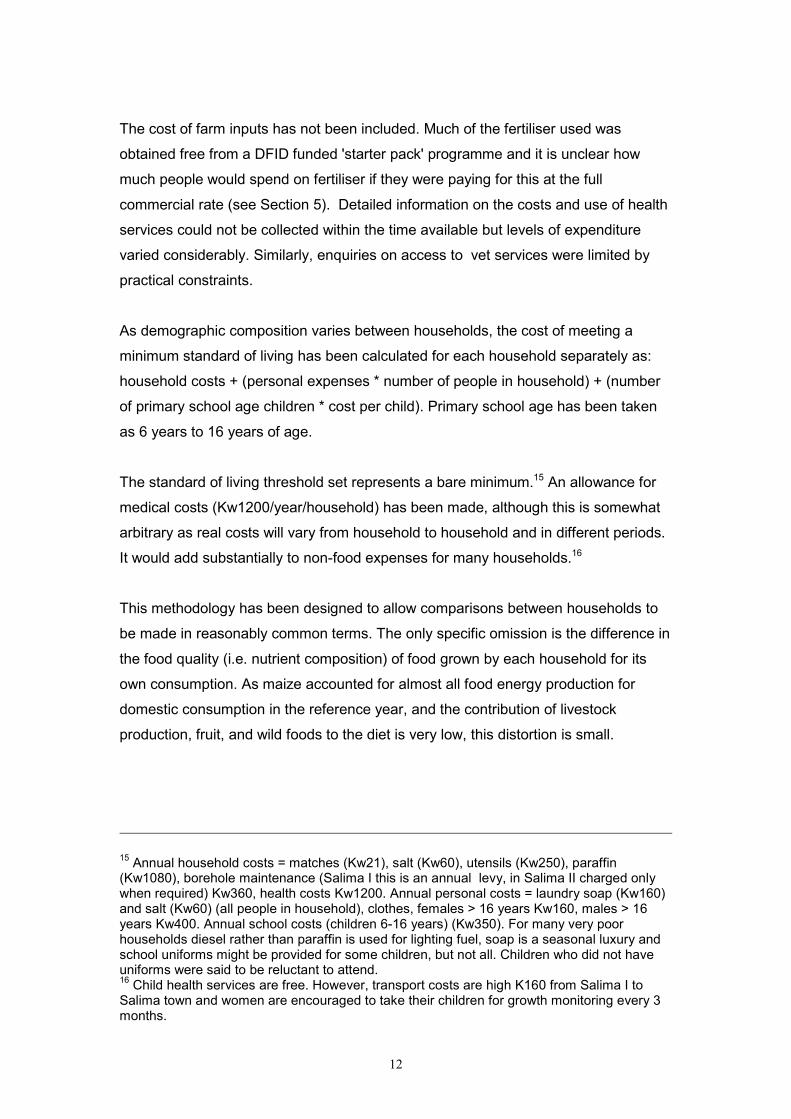
The cost of farm inputs has not been included. Much of the fertiliser used was

obtained free from a DFID funded 'starter pack' programme and it is unclear how

much people would spend on fertiliser if they were paying for this at the full

commercial rate (see Section 5). Detailed information on the costs and use of health

services could not be collected within the time available but levels of expenditure

varied considerably. Similarly, enquiries on access to vet services were limited by

practical constraints.

As demographic composition varies between households, the cost of meeting a

minimum standard of living has been calculated for each household separately as:

household costs + (personal expenses * number of people in household) + (number

of primary school age children * cost per child). Primary school age has been taken

as 6 years to 16 years of age.

The standard of living threshold set represents a bare minimum.15 An allowance for

medical costs (Kw1200/year/household) has been made, although this is somewhat

arbitrary as real costs will vary from household to household and in different periods.

It would add substantially to non-food expenses for many households.16

This methodology has been designed to allow comparisons between households to

be made in reasonably common terms. The only specific omission is the difference in

the food quality (i.e. nutrient composition) of food grown by each household for its

own consumption. As maize accounted for almost all food energy production for

domestic consumption in the reference year, and the contribution of livestock

production, fruit, and wild foods to the diet is very low, this distortion is small.

15 Annual household costs = matches (Kw21), salt (Kw60), utensils (Kw250), paraffin(Kw1080), borehole maintenance (Salima I this is an annual levy, in Salima II charged onlywhen required) Kw360, health costs Kw1200. Annual personal costs = laundry soap (Kw160)and salt (Kw60) (all people in household), clothes, females > 16 years Kw160, males > 16years Kw400. Annual school costs (children 6-16 years) (Kw350). For many very poorhouseholds diesel rather than paraffin is used for lighting fuel, soap is a seasonal luxury andschool uniforms might be provided for some children, but not all. Children who did not haveuniforms were said to be reluctant to attend.16 Child health services are free. However, transport costs are high K160 from Salima I toSalima town and women are encouraged to take their children for growth monitoring every 3months.

13

Modelling the impact of changes affecting a household

A cross sectional survey can only give a snapshot of recent economic conditions. In

fact, the absolute and relative level of household income will vary over time, as

changes occur, both within the household (e.g. births, illness and deaths, the

adoption of orphans) and in the external context to which all households relate (e.g.

changes in crop production and crop and input prices, availability of food aid etc).

However, the data set we collected can be used to simulate the impact of some

external changes on current household disposable income and standard of living: in

other words, it can be used to model the vulnerability of households to specified

changes. This is done by recalculating disposable income under the stated changed

conditions (for example, with and without food aid). A simple example is given in

Annexe 2.17 In practice this involves a large amount of calculation, and software was

written for the analysis.

5. Findings and analysis

Population

Orphans have been defined as children under the age of 17 years who have lost one

or both parents. 18

Grandparent headed households included one or two grandparents.

The population of Salima I is 683 (complete census) and Salima II 168 people. Figure

1a shows the recorded population of each village grouped by one-year divisions from

birth to 79 years of age, and all ages above 79 years, distinguishing male and female

orphans. Note that younger ages are probably accurately recorded to the nearest

year, but some older people did not always confidently know their ages and there is

an element of estimate for older age groups. The data is summarised in Figure 1b

and Table 1. 17 The approach could also be used in a longitudinal study to monitor and quantify changeover time, including responses to external shocks and changes in household demography.18 A cut-off of 17 years was used, rather than the 18years recommended by WHO, to maintainconsistency with earlier studies. The use of a higher threshold makes little difference to theresults. Older people have not been included as dependants as age did not seem to be a barto full economic activity.

14

Salima I: Population

-30 -20 -10 0 10 20 300-1

6-7

12-13

18-19

24-25

30-31

36-37

42-43

48-49

54-55

60-61

66-67

72-73

78-79

Age

, yea

rs

Number in group

Male - OrphanMaleFemale - OrphanFemale

Salima II: Popula tion

-10 -5 0 5 100-1

5-6

10-11

15-16

20-21

25-26

30-31

35-36

40-41

45-46

50-51

55-56

60-61

65-66

70-71

75-76

>80

Age

Num ber in group

Male - OrphanMaleFem ale - OrphanFem ale

Figure 1a. Population of Salima I and Salima II by 1 year age groups.

15

Salima I: Population

-100 -50 0 50 100

0-5

10-15

20-25

30-35

40-45

50-55

60-65

70-75

80+

Age

, 5 y

ear i

nter

vals

Number in group

Male - OrphanMaleFemale - OrphanFemale

Salima II: Population

-20 -10 0 10 20

0-5

5-10

10-15

15-20

20-25

25-30

30-35

35-40

40-45

45-50

50-55

55-60

60-65

65-70

70-75

75-80

80+

Age

, 5 y

ear i

nter

vals

Number in group

Male - OrphanMaleFem ale - OrphanFem ale

Figure 1b. Population of Salima I and Salima II by 5 year age groups.

16

Orphans make up 8.9% and 10.7% of the total population of Salima I and Salima II

respectively, and 15.6% and 21.2% of the under-17 year population. In Salima I,

orphan girls outnumber orphan boys by 1.8: 1. In Salima II the ratio is reversed

(1:3.5)19.

Table 1 Population CategoriesSalima I Salima II

Male Female Total Male Female TotalOrphans 22 39 61 14 4 18

All other people 313 299 612 69 81 150

Total 335 338 673 83 85 168

Children under 17years age

197 195 392 44 41 85

In Salima I, 61orphans were recorded in 32 households (22.5%) out of a total of 142

households. Twenty-two (15.5%) households were female headed and 20 (14%)

headed by one or two grandparents. Seven of the 20 grandparent headed

households are also female headed. Orphans were recorded in 4.2% of female

headed household (N=6.); 5.6% of grandparent headed households (N=8); and 1.4%

of female headed grandparent households (N=2).

In Salima II, orphans were resident in 9 (29%) of all (N=31) households. Two

households (6.5%) were female headed and 3 (9.7%) were grandparent headed.

One grandparent headed household was also female headed. Orphans were

recorded in all grandparent headed households.

The average household size in Salima I was 5.3 people and in Salima II 4.6 people.

School attendance

In Salima I, 83% of all children aged 6-16 years were attending school (male 85%,

female 80%) and in Salima II, 66.7% of children aged 6-16 years were attending

school (male 69%, female 58%).20

19 An excess of girls was found in our studies in Swaziland and Mozambique and is consistentwith other reports. The reason for the reverse ratio in Salima II is unclear. The question 'whathappens to boys?' requires further rigorous investigation. The assumption is that many leavetheir communities prematurely and migrate to urban areas.20 The reasons for non attendance were not researched in depth, but interviews suggestedthat lack of money for uniforms deters a proportion of poorer children from attending.

17

Sources and levels of household income 21

Household income in the reference year was to some extent distorted by the

distribution of food aid. In the following section, results have been presented as these

were recorded, including food aid as a source of income.

A list of all sources of food and cash income is given in Annexe 2. Table 2 shows the

respective contributions of the main categories of income to total village food and

cash income. Food for consumption makes up a little over half of the cash value of all

income in both villages (Salima I 58% Salima II 52%).

Crops produced for consumption were chiefly maize, groundnuts and beans. Non-

relief gifts of cash and food were all gifts from kin. Food payments in kind were made

in maize. Wild foods make only a very small contribution to the diet and are highly

seasonal. These include a range of wild fruits and plants of low energy value and

Baobab fruit and wild Okra. Mangoes were classified as a cultivated crop. Aside

from some seasonal fishing (in Salima II) the only wild animal hunted, excepting

occasional birds, is the field mouse, which is caught in large numbers in fields and

granaries.22 Almost no foods of animal origin are consumed.

Table 2 Sources of income as food and cash

Salima I Salima IISource of income as food % of all food income(as food energy, Kcal)Crops 53.2 76.7Livestock and livestock products 1.6 2.1Payment in kind 3.6 7.5Non-relief gifts 10.9 3.5Relief 29.6 9.6Wild foods 1.2 0.6

21 Note that the economic analysis described in the following paragraphs is based on a 50%sample in Salima I (every even numbered household) and all households in Salima II.22 Examples of all wild foods were obtained, but not all could be identified. For items thatwere of very low energy content e.g. a fruit eaten for its sweet taste, but with virtually noedible flesh, the energy value was estimated. The energy values of the major items (chieflyOkra, Baobab fruit) were known. Mice were obtained in edible form and weighed, and theirenergy value estimated from values for other game.

18

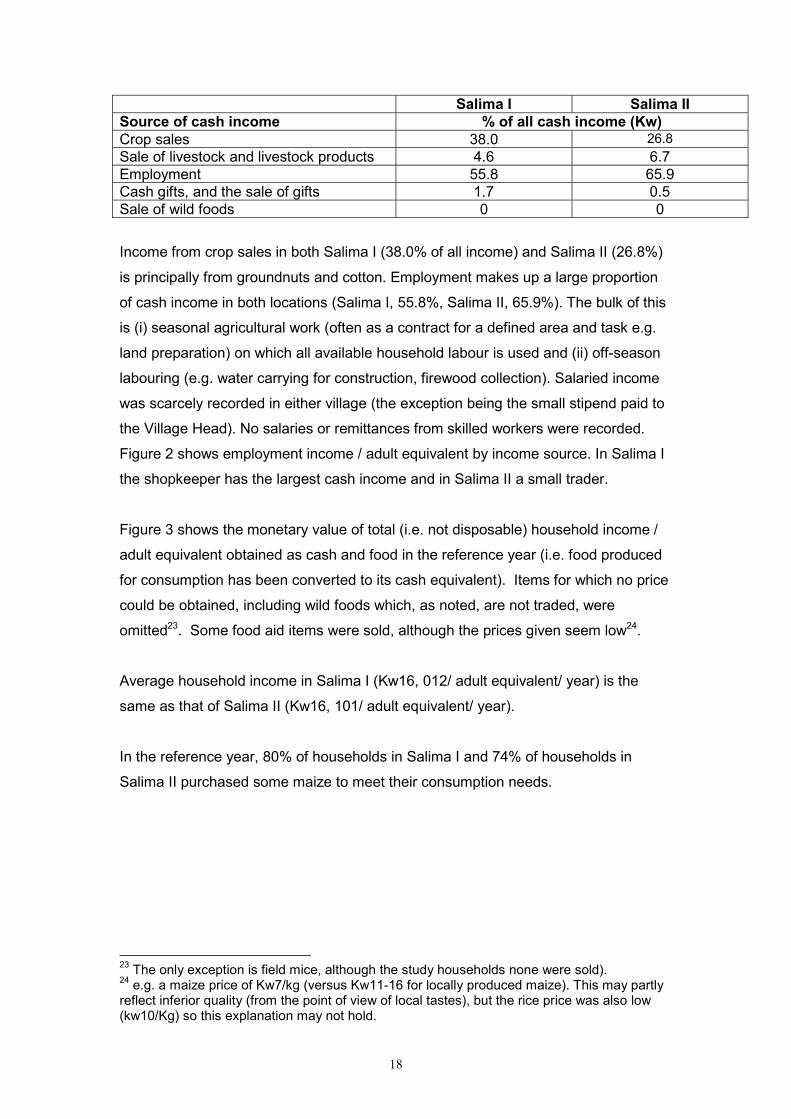
Salima I Salima IISource of cash income % of all cash income (Kw)Crop sales 38.0 26.8Sale of livestock and livestock products 4.6 6.7Employment 55.8 65.9Cash gifts, and the sale of gifts 1.7 0.5Sale of wild foods 0 0

Income from crop sales in both Salima I (38.0% of all income) and Salima II (26.8%)

is principally from groundnuts and cotton. Employment makes up a large proportion

of cash income in both locations (Salima I, 55.8%, Salima II, 65.9%). The bulk of this

is (i) seasonal agricultural work (often as a contract for a defined area and task e.g.

land preparation) on which all available household labour is used and (ii) off-season

labouring (e.g. water carrying for construction, firewood collection). Salaried income

was scarcely recorded in either village (the exception being the small stipend paid to

the Village Head). No salaries or remittances from skilled workers were recorded.

Figure 2 shows employment income / adult equivalent by income source. In Salima I

the shopkeeper has the largest cash income and in Salima II a small trader.

Figure 3 shows the monetary value of total (i.e. not disposable) household income /

adult equivalent obtained as cash and food in the reference year (i.e. food produced

for consumption has been converted to its cash equivalent). Items for which no price

could be obtained, including wild foods which, as noted, are not traded, were

omitted23. Some food aid items were sold, although the prices given seem low24.

Average household income in Salima I (Kw16, 012/ adult equivalent/ year) is the

same as that of Salima II (Kw16, 101/ adult equivalent/ year).

In the reference year, 80% of households in Salima I and 74% of households in

Salima II purchased some maize to meet their consumption needs.

23 The only exception is field mice, although the study households none were sold).24 e.g. a maize price of Kw7/kg (versus Kw11-16 for locally produced maize). This may partlyreflect inferior quality (from the point of view of local tastes), but the rice price was also low(kw10/Kg) so this explanation may not hold.

19

Salima I: Household cash income/ adult equivalent by source

-10,000

0

10,000

20,000

30,000

40,000

50,000

60,000

70,000

1 5 9 13 17 21 25 29 33 37 41 45 49 53 57

Household: 1 = poorest

Kw

Cash gifts

Cash employment

Livestock & livestock productsalesCrop sales

Salima II: Household cash income/ adult equivalent by source

-10000

0

10000

20000

30000

40000

50000

60000

1 4 7 10 13 16 19 22 25 28 31

Household: 1 = poorest

Kw

Cash gifts

Employment

Livestock & livestock productsalesCrop sales

Figure 2. Household cash income/adult equivalent by source, Salima I and Salima II.Shown in ascending order of disposable income

20

Salima I. Total value of household income/ adult equivalent.

0

20,000

40,000

60,000

80,000

100,000

120,000

140,000

1 6 11 16 21 26 31 36 41 46 51 56

Household: 1 = poorest

Kw

/ yea

r

Cash incomeCash value of all food income

Salima II: Total value of all income/ adult equivalent

0

20,000

40,000

60,000

80,000

100,000

120,000

1 4 7 10 13 16 19 22 25 28 31

Household: 1 = poorest

Kw Cash income

Cash value of all food income

Figure 3 Total income as cash value of food and cash Salima I and Salima II.Omits the value of wild foods and some relief foods. Shown in ascending order ofdisposable income

21

Livestock holdings

Livestock holdings at both sites were very low. The reasons for this included (i)

livestock sales during the 2001/2002 famine 25; (ii) the theft of larger stock; (iii) the

loss of animals to disease (which was identified from interviews as the main cause.)

Large numbers of poultry were lost to Newcastle disease in 2003, cattle to foot-and-

mouth disease, and pigs and goats to unspecified epidemic diseases. Animals are

not generally vaccinated, although for a charge, some vaccines and veterinary

services are available 26. 71% of all households in Salima I and 61% of households in

Salima II held some livestock. Average household livestock holdings are given in

Table 3.

Table 3 Livestock holdings

Goat Pig Chickens Ducks Guinea fowlAverage number of animals/ household

Salima I 1.0 0.8 3.8 0.5 0.1Salima II 0.0 0.44 0.56 5.2 0.0

Disposable income and the standard of living

Figure 4 shows disposable income/ adult equivalent by household (i.e. cash

remaining after household food costs have been met) in ascending order of

disposable income. Households that fall below the defined minimum standard of

living are shown in red (see section 4). In Salima I, 33.9% of all households fall

below the defined poverty threshold and in Salima II 38.7 %.

In Figure 4, several of the poorest households are shown with a negative disposable

income. This is to say that in the reference year, the recorded household food and

cash income was insufficient to meet the household’s food needs. All of these

households were observed to be very poor. The explanation includes: (i) a lower

actual level of food consumption than was used in calculation; (ii) possibly some

under-reporting of small income sources, particularly charitable gifts and off-season

Ganyu; (iii) the possibility that the household was using savings and other capital to

survive, or (iv) the household was in fact failing. 25 In which some people in Salima I died (see “Waiting for food in Salima”).26 Cattle theft was common (apparently sponsored by a known individual in Salima). Althoughtheft is not now considered a major problem it remains one reason for not investing in cattle.Although the question was not systematically asked of all households, people do not routinelyvaccinate animals, if at all. In Salima II Guinea fowl are preferred to chickens because of their

22

disease resistance: chickens are used to incubate Guinea fowl eggs, which are sold at apremium.

Salima I: Disposable income/ adult equivalent and the standard of living

-10,000

0

10,000

20,000

30,000

40,000

50,000

60,000

70,000

1 6 11 16 21 26 31 36 41 46 51 56

Household: 1 = poorest

Kw < Standard of living threshold

> Standard of living threshold

Salima II: Disposable income/ adult equivalent and the standard of living

-10,000

0

10,000

20,000

30,000

40,000

50,000

60,000

1 4 7 10 13 16 19 22 25 28 31

Household: 1 = poorest

Kw < Standard of living threshold

> Standard of living threshold

Figure 4. Salima I and Salima II. Household disposable income/adult equivalent,showing households below the standard of living threshold. Shown in ascendingorder of disposable income

23

Disposable income is very unequally distributed, ranging from less than zero to Kw

5,375/ adult equivalent/year and in Salima I and Kw 5,184/ adult equivalent/ year in

Salima II (US$1 = approximately Kw100 at the time of the survey)

Disposable income and orphan residence

Figure 5 shows disposable income/ adult equivalent and identifies those households

with resident orphans in female headed, grandparent headed and female

grandparent headed households.

Salima II: Disposable income/ adult equivalent & orphans in different household categories

-10000

0

10000

20000

30000

40000

50000

60000

1 3 5 7 9 11 13 15 17 19 21 23 25 27 29 31

Household: 1 = poorest

Kw

Female & gradparent headed +orphanGrandparent headed + orphan

Female headed +orphan

Orphan

No orphans

Figure 5. Salima I and Salima II. Household disposable income/adult equivalentin ascending order of disposable income, showing households with orphans.

Saliama I: Disposable income/adult equivalent & orphans in different categories of household

-10,000

0

10,000

20,000

30,000

40,000

50,000

60,000

70,000

1 5 9 13 17 21 25 29 33 37 41 45 49 53 57

Household: 1 = poorest

Kw

Grandparent headed + orphanFemale headed +orphanOrphanNo orphans

24

Table 4 Disposable income, orphan residence, female and grandparent headedhouseholds

Salima I Salima IIPoorest 30households

Richest 29households

Poorest 16households

Richest 15households

Orphan households (%, number) 30%(9) 17%(5) 50%(8) 13.3%(2)Number of orphans 22 7 12 3Average number orphans/ orphanhousehold

2.4 1.4 1.5 1.5

Female headed households (%, number) 23.3%(7) 6.9%(2) 12.5%(2) 0%(0)Number of female headed householdswith orphans

1 1 1

Grandparent headed households (%,number)

13.3%(4) 10.3%(3) 12.5%(2) 6.6%(1)

Grandparent headed households withorphans

2 0 2 1

At both sites (Table 4) more households with orphans fell in the poorer part of the

income distribution. In Salima I, but not in Salima II, the average number of orphans

per orphan household was greater in the poorer group. More female-headed

households fell in the poorer group, but orphans were found in only 3 female headed

households from a total (both sites) of 11 female headed households27. In the Salima

I sample, orphans were found in 2 out of 4 grandparent headed households in the

poorer group, and not in grandparent headed households in the better off group. In

Salima II all grandparent headed households had resident orphans.

The dependency ratio

The dependency ratio (calculated as the ratio of people under 17 years of age:

number over 17 years age28) and those households with resident orphans are shown

in Figure 6, in order of disposable income. Although the trend is for poorer

households to have higher ratios, at neither site is there a significant relationship

between the dependency ratio and household disposable income (Salima I r2 =

0.0657, Salima II r2 = 0.1911, p>0.1). Grouping the data into the poorest and richest

suggests a higher dependency ratio in poorer households, particularly in Salima II

(Salima I, 1.98 in the poorest 30 households, 1.64 in the richest 29); Salima II, 1.43 in

the poorest 16 households, 0.73 in the richest 15.). As would be expected,

27 Note that households were female headed through divorce as well as widowhood.28 See footnote 16.

25

households with orphans have a higher average ratio (Salima I, 2.06, Salima II, 1.64)

than households without (Salima I, 1.41, Salima II, 0.83).

Salima I: Ratio of children < 17 years age : people > 17 years age

0

0.5

1

1.5

2

2.5

3

3.5

4

4.5

1 4 7 10 13 16 19 22 25 28 31 34 37 40 43 46 49 52 55 58

Household: 1 = poorest

Ratio Household with orphans

Household without orphans

Salima II: Ratio children < 17years : people > 17 years age

0

0.5

1

1.5

2

2.5

3

3.5

1 2 3 4 5 6 7 8 910111213141516171819202122232425262728293031Household: 1 = poorest

Ratio Household with orphans

Household without orphans

Figure 6. Salima I and Salima II. Household dependency ratio, showing householdswith orphans. Shown in ascending order of disposable income

26

However (Figure 6) in Salima I there is no obvious relationship between disposable

income, the dependency ratio and the presence of orphans in a household. Of the 30

poorest households, non-orphan and orphans households have a similar

dependency ratio (1.94 and 2.07).

In Salima II, almost all orphan households fall the poorest half of the wealth

distribution. Within this group, the poorest 7 orphan households have a higher

dependency ratio (1.68) than the poorest 8 non-orphan households (1.20).

The impact of food aid on disposable income and food aid targeting criteria

Food aid in the reference year made a substantial contribution to the total income

and disposable income of some households (Figure 7). Recalculating disposable

income omitting food aid as a source of income, suggests that in Salima I, food aid

increased average household disposable income by 6.9% and in Salima II by 5.6%.

This calculation assumes that had food aid not been distributed, other household

economic activities and income would have remained the same. This seems likely to

be broadly true i.e. for most households it seems unlikely that the receipt of a small

amount of food aid would act as an economic disincentive or incentive, but is untrue

for some of the very poorest households. For example in Salima I an ill single woman

household with no other source of income was wholly dependent on food aid and

small charitable gifts and we cannot know what would have happened if food aid had

not been supplied.

Note that recalculating disposable income omitting food aid alters the relative

disposable income of each household, as households that received significant

amounts of food aid become relatively poorer. In the example given of an ill single

woman household in Salima I this household is, omitting food aid, the poorest

household (with effectively no income); with a full ration and some charitable gifts,

the household is the 20th poorest. Omitting food aid increases the proportion of all

households below the standard of living threshold, from 33.8% to 42.4% in Salima I

and from 38.7% to 41.9% in Salima II 29. Omitting food aid also reduces the number

of households with food income in excess of household requirement (See Section 4);

in Salima I, this falls from 16.9% to 6.8% of households and Salima II, from 25.8% to

22.5% of households.

27

Omitting food aid represents more fairly the actual pattern of need prior to the food

aid distribution.

Salima I. Contribution of food aid to household disposable income/ adult equivalent. Orphan households in red

0

500

1000

1500

2000

2500

1 3 5 7 9 11 13 15 17 19 21 23 25 27 29 31 33 35 37 39 41 43 45 47 49 51 53 55 57 59

Household: 1 = poorest

Kw

Salima II: Contribution of food aid to household disposable income/adult equivalent

0

200

400

600

800

1000

1200

1 2 3 4 5 6 7 8 9 10 11 12 13 14 15 16 17 18 19 20 21 22 23 24 25 26 27 28 29 30 31

Household: 1 = poorest

Kw

Figure 7. Salima I and Salima II. Contribution of food aid to householddisposable income. Shown in ascending order of disposable income calculatedwithout food aid. In Salima II households 2 and 3 were orphan householdswhich did not receive food aid.

28

Who received food aid?

The criterion for the supply of food aid was that this should be distributed to orphan

and vulnerable households, the CBO being given some latitude in the definition of

vulnerability. The following section describes the households that received food aid

where the level of disposable income has been calculated without food aid i.e.

simulating the situation before food aid was distributed. The standard of living

threshold is used as a measure of vulnerability, but this is not necessarily the

criterion used by the CBO.

Table 5 Households receiving food aid

Salima I Salima II% (number of households)

% all households with orphans receiving food

aid

63.6% (11) 20%(2)

% all non-orphan households receiving food

aid

43%(19) 33%(7)

Households < Standard of living threshold 42.5%(25) 41.9% (13)

% households with orphans below Standard

of living threshold receiving food aid

100%(7) 22% (2)

% non- orphan households below Standard

of living threshold receiving food aid

32%(8) 33%(2)

In Salima I, 60% (15 of 25) households below the standard of living threshold

received food aid. All 7 households with orphans falling below the standard of living

threshold received aid. 44% of households above the standard of living threshold

received food aid (15 of 34 households). 50% of households with orphans (4 of 7)

above the standard of living threshold received aid.

In Salima II of 13 households below the standard of living threshold, 4 (31%)

received food aid. Of 7 households with orphans below the standard of living

threshold, 2 received aid. Three households with orphans above the threshold did not

receive aid.

29

Pre-school feeding

In Salima I, where 25 households received pre-school food, pre-school feeding

increased average disposable income by 2.7%. In Salima II, 10 households received

pre-school meals which contributed 1.8% to average disposable income. 30

Characteristics of households below the standard of living threshold

Table 6 shows the characteristics of those 25 households in Salima I which fall below

the standard of living threshold, calculated omitting food aid.

Table 6 Characteristics of households below the standard of living threshold,Salima I

Salima I. Household characteristics.Illness Orphan/s Female

headedDivorced Grand

parentheaded

Othersocial/economic

Dependencyratio

Household1(poorest) X X 02 X X 03 X X 24 X 35 X X 46 X 27 X 2.58 X 2.59 X X 110 X 1.2511 X 112 X X 413 X 214 X 0.515 X X 316 X X 417 218 X 319 X 1.720 X 221 X 1.722 X 2.523 X 2.524 X 025 X 0.75 30 Both CBOs organising pre school activities included members from adjacent villages.Salima I pre school was situated in the centre of the community; Salima II preschool at a shortdistance.

30

In both the two poorest households the (female) head is ill. Divorced women head

four households. Other social/economic detail includes a household in which the

husband only visits home irregularly and which also supports a sister’s (non-orphan)

children. For the most part the poorest households are those with low incomes and a

large number of dependants.

Land use

In Salima I, where only upland crops are grown, most households reported unused

land in the reference year. In Salima II, where most households have access to

dambo (i.e. riparian) land, which is better watered and will produce a reasonable

return without fertiliser, it was found that all dambo was cultivated, either by the

owner or a tenant. In Salima II, as in Salima I, a variable proportion of the upland

available to each household was cultivated.

Figure 8 shows, by household, the proportion of available upland cultivated in the

reference year and Figure 9 the proportion of cultivated land put to the main crops

grown. In Salima I the greatest proportion of land was put to the cultivation of maize,

cotton and groundnuts; in Salima II cash crops are much less prominent.

In Salima I, households with orphans (N=15) and without orphans (N=44) had

access to a similar amount of land (with orphans 6.25 acres, without orphans 6.47

acres) and, on average, cultivated a similar proportion of this (with orphans 61.6%,

without 62.6%). In Salima II households with orphans (N=10) have access to less

land (2 acres) than non-orphan households ((N=21) 2.85) and cultivate on average a

larger proportion of this (90.7%) than non orphan households (68.9%), although a

similar area (with orphans 1.78 acres, without 1.75 acres).

31

Salima I. Percent of all available land cultivated

0

20

40

60

80

100

120

1 4 7 10 13 16 19 22 25 28 31 34 37 40 43 46 49 52 55 58

Household: 1 = poorest

%

Orphan householdsNon-orphan households

Salima II. Percent of all available land cultivated

0

20

40

60

80

100

120

1 3 5 7 9 11 13 15 17 19 21 23 25 27 29 31

Household: 1 = poorest

%

Orphan householdsNon-orphan households

Figure 8. Salima I and Salima II. Percentage of all land cultivated. Householdswith orphans in red. Shown in ascending order of disposable income

32

Salima I. Percent of all land used for different crops

0

20

40

60

80

100

120

1 4 7 10 13 16 19 22 25 28 31 34 37 40 43 46 49 52 55 58

Household: 1 = poorest

%

Sweet potatoesBeansGroundnutsCottonMaize

Salima II: Percent of all cultivated upland used for different crops

0

20

40

60

80

100

120

1 3 5 7 9 11 13 15 17 19 21 23 25 27 29 31

Household: 1 = poorest

%

Sweet potatoesTobaccoBeansCottonGroundnutsMaize

Figure 9. Salima I. Percentage of all cultivated land used for different crops. SalimaII Percentage of all upland used for different crops. Shown in ascending order ofdisposable income

33

The reason for the lower landholding by orphan households in Salima II is unclear.

Households with orphans in Salima II are relatively poor: however, taking the 15

poorest households and comparing the non-orphan and orphan households suggests

that a smaller land holding is specific to households with orphans (non-orphan 2.93

acres (n=7), orphan = 1.86 acres (N=8)), and is not simply a feature of household

poverty.31

In Salima I, the 29 better off households have access to slightly more land (3.1 acres)

then the poorest 30 households (2.4 acres). In Salima II the poorest 15 households

have access to 2.48 acres of upland, the better off 16 households 2.66 acres.

The reasons given for not cultivating all of the available land varied (e.g. it included

temporary illness) but was chiefly given as a lack of cash to purchase inputs and the

high input price.

Input use and maize returns

All farmers asked gave the high cost of fertiliser for use on upland maize as their

greatest concern. The only other input identified was pesticide for cotton, the cost of

which was low (1 bottle / acre @ Kw10/ bottle).

Farmers obtained fertiliser from starter packs 32, on credit, and/or on the open

market, including the purchase of starter packs from other recipients. Fertiliser prices

varied (from zero for starter packs to Kw 44/ kg for some commercial fertiliser). Some

farmers obtained fertiliser from multiple sources and in some cases starter packs

were subdivided. The amount of fertiliser used/ acre and its cost varied widely,

depending in each case on the particular source or combination of sources.

57% of households in Salima I and 61% of households in Salima II used some

fertiliser in the reference year.

In Salima I, the quantity of fertiliser obtained by households with and without orphans

was similar (orphan 30.5kg/acre, non-orphan 30 kg/acre). The poorest 30

households used less fertiliser (20.9kg/acre) than the richest 29 (39.7kg/acre). In 31 There is some indication that this may be due to widows returning to their home communityand receiving a smaller than average allocation of land. However, historical analysis oflandholdings was outside the scope of this study

34

Salima II orphan households used substantially less (12kg/acre) than non-orphan

households (36.2Kg/acre). The poorest 15 households used less (20kg/acre) than

the richest 16 households (36.1 kg/acre).

The quantity of fertiliser used/acre and the maize return / acre are correlated (Salima

I, r2 = 0.4741, p< 0.01; Salima II, r2 = 0.3205, p<0.1). Combining the two data sets

(r2 = 0.4007, N = 79, p< 0.0.1) and excluding households which did not cultivate, a

linear regression suggests that fertiliser use accounts for approximately 40% of the

variation in yield. The remaining variation is due to a variety of other factors (flooding,

damage by animals, pests). From the regression, using no inputs, the average yield

would be 135 kg maize/ acre, and at the maximum level of fertiliser use recorded

(110kg/acre) the average yield would be 529 Kg maize/ acre33.

Figure 10 shows the net return on fertiliser use calculated using the actual rate of

fertiliser/ acre and the actual maize yield/ acre recorded for each household, at two

different levels of fertiliser price (i) Kw 44/kg i.e. roughly the commercial rate (ii) Kw

22/ Kg, ie half the commercial rate. The maize price has been held at Kw13.5/ kg (the

mid year price used in this analysis). A doubling of the maize price (Kw27/kg) would

achieve the same net return as a halving of fertiliser price.

This suggests that under the growing conditions in the reference year, at the

commercial fertiliser price, a farmer would maximise the chance of obtaining some

return by using no fertiliser, or very little fertiliser. At rates of fertiliser use up to

20kg/acre, the risks would have been low and net return positive, although the

average return would be only slightly greater (Kw 1907/acre) than using no fertiliser

(Kw1695/ acre). Over the entire recorded range of fertiliser use, about one-third of all

farmers using fertiliser would have lost money and at rates of fertiliser use above

60kg/ acre all would have done so at the current commercial fertiliser price.

In reality the situation would be complicated by seasonal variations in maize price.

Poorer farmers would tend to get a lower price i.e. they would have no choice but to

sell or consume their maize production in a period when prices are low. Better-off

farmers might be able to retain a surplus and sell at a higher pre-harvest price.

32 26 were distributed in Salima II in 2003; information not available for Salima I33 Local information was that using the recommended level and types of inputs (in total 200kg/acre) returns as high as Kg 2,000/acre can be obtained).

35

Farmers in Salima II estimated that that the 2005 pre-harvest maize price will be

approximately Kw18/ kg, at which rate returns on fertiliser use would improve.

Salima I & Salima II combined: upland maize, net return/acre @ maize price = Kw13.5/kg & fertiliser price = Kw44/Kg

-2,000

-1,000

0

1,000

2,000

3,000

4,000

5,000

6,000

7,000

1 5 9 13 17 21 25 29 33 37 41 45 49 53 57 61 65 69 73 77

Household

Kw

Input cost/ acreNet return/acreLinear (Net return/acre)

Salima I & Salima II combined: upland maize, net return/acre @ maize price = Kw13.5/kg & fertiliser price = Kw22/Kg

0

1,000

2,000

3,000

4,000

5,000

6,000

7,000

1 5 9 13 17 21 25 29 33 37 41 45 49 53 57 61 65 69 73 77

Household

Kw

Input cost/ acreNet return/acreLinear (Net return/acre)

Figure 10. Salima I and Salima II. Simulated net return on upland maize cultivation,using observed rate of fertiliser use and maize return (kg/ acre) at different fertiliserprices.

36

6. Summary of findings

Both villages are characterised by very high levels of poverty and the most basic,

comfortless conditions of life. Households with orphans, female-headed households

and grandparent headed households with and without orphans, tend to be relatively

poorer than non-orphan households. In Salima II households with orphans were

distinguished by less access to land, (although they cultivated a similar amount of

land in the reference year); using less fertiliser and receiving less food aid. The

reasons for this are not entirely clear, but may be due to the fact that some settled in

the village after bereavement.

A large proportion of the poorest households do not fall into the category of either

female headed or grandparent headed or orphan, and many of the female-headed

households are the result of divorce rather than bereavement. In the two

communities, poverty is characterised by:

(i) An absolute or relative lack of household labour in an economy where income

for poor households depends entirely on manual labour for both domestic

production and income from paid employment. This is variously due to a high

dependency rate; illness and infirmity, the lack of a male (or female) adult

household member, or a combination of these. To the extent that orphans are

a proxy for HIV/AIDS and contribute to household poverty, this group makes

up about 20% of those households below the standard of living threshold

(Salima I).

(ii) A lack of money to acquire fertiliser and livestock.

(iii) The poor returns and high risks associated with fertiliser use at current

fertiliser/maize prices.

(iv) Poor (virtually no) returns from livestock, and the loss of capital and

investment in livestock, primarily resulting from a lack of access to effective

veterinary services34.

(v) Low cash crop prices, particularly for cotton.

This analysis suggests that the presence of orphans is not a reliable household level

indicator for targeting assistance to the poorest. It also casts doubt on the causal link

34 We were unable to go into this in detail, but the impression was that the charges were adeterrent. The potential returns on some livestock are substantial and the subject would meritfurther investigation.

37

between HIV/AIDS and declining levels of cereal production observed in many parts

of southern Africa.

We did not gather detailed retrospective information on changes in individual

household economy that would be needed to quantify the economic impact of

HIV/AIDS. However, from key informant interviews with widows and others, it is clear

that, following a bereavement, households in the study communities change

demographic structure in a variety of ways e.g. bereaved women may follow

traditional practice and marry a brother in law, or they may choose to continue alone;

bereaved men may remarry, orphans move into the households of kin etc. Rigorous

analysis of the economic implications of these changes requires more detailed

demographic information than was obtained on this study. Interviews with

households and the understanding of household economy obtained on the study do,

nevertheless challenge assumptions (e.g. FAO 2004) of a steep descent into poverty

following the loss of active adult male labour (from bereavement or divorce), or the

adoption of children by grandparents or others into a household.

This is because (i) household heads can to some extent compensate for the lost

income by expanding their own workload, albeit at some personal and social cost

(e.g. during periods of high seasonal workload, time for child care is lost, and older

household heads continue working in order to maximise income). (ii) In cases of

bereavement or divorce, the lost income is partly compensated by a fall in household

costs. (iii) Some women headed households received increased support from

relatives. The income of such households would of course be more vulnerable, e.g.

to illness, than households with two active adults and in this economy it would be

expected that in general such households would become poorer.

The cost of supporting orphans

To illustrate the financial cost of caring for orphans, we have calculated for Salima I

the total annual costs of maintaining all children who have lost one or both parents.

The basic standard of living criteria set out in section 5 have been used. The costs

per child, and for all (61) orphans in Salima I are set out in Table 7.

38

Table 7 Costs of maintaining children, to meet minimum standard of livingcriteria.Item Cost per

childCost for all (61)orphans in Salima I

Food * Kw 2,554 Kw 155,794

School costs Kw 350 Kw 21,350

All non-food costs,

including school costs

Kw 570 Kw 34,770

Total food and non food

costs per year

Kw 3124 Kw 190,564

(approx US$1,900 )

*Assumes that food, whether produced or purchased costs Kw13.5/ kg i.e. the maize

price used in the analysis.

7. The potential impact of policy and programme interventions on the pooresthousehold

To explore the practical inferences that can be drawn from this analysis, we have

included a final section showing examples of the changes to disposable income that

would result from a range of possible policy changes and programme interventions,

with particular emphasis on the benefits which would accrue to the poorest

households.

Three policy interventions have been selected either because these are current in

Malawi, or are internationally topical:

(i) Fertiliser prices

(ii) Maize prices

(iii) Cotton prices

and three programme interventions

(i) The impact of general food distribution

(ii) School feeding

(iii) Cash distribution.

The aim here is to illustrate only the size and pattern of the immediate changes in

disposable income that would result from each policy or programme change. Any

39

change that substantially increases disposable income may lead to increased

consumption and/or create an opportunity for a household to invest in further

productive activity and create employment opportunities. For example, a sustained

reduction in fertiliser price or increase in maize price would be expected to increase

investment in maize production, at least by better off farmers who could afford the

inputs and absorb the risk (Section 5) and might also benefit the poor households

with labour by increasing the availability of, or returns from, day labour. Similarly, in

Salima I several households (around 8-10) were investing in building brick houses,

as a result of better returns on cotton in 2002/2003, thus creating more day labour

opportunities (water carrying, brick making, labouring, plank cutting etc).

The examples have been developed only for Salima I. The poorest households are

defined as those falling below the standard of living threshold, including food aid (see

Section 4).

Maize, Cotton and Fertiliser price

To illustrate the importance of maize production to household disposable income and

standard of living, disposable income has been recalculated assuming that

households used the same amount of land as in the reference year, and obtained a

return of 580kg maize/acre (equivalent to the largest rate of return recorded on the

survey). 35 The effect of this would be to increase average disposable income (all

households) in Salima I by 24.3%, reduce the proportion of households falling below

the standard of living threshold from 33.8% to 20.3% and increase the disposable

income of households below the standard of living threshold by an average of

Kw1651/adult equivalent/year (see Figure 11). All households would benefit except

for one household that did not cultivate because of illness. This demonstrates the

substantial impact on income and living standards that could be achieved by

improving the returns on maize production.

35 Note that it is impossible to estimate the impact of fertiliser use on household disposableincome as households in Salima I already used some fertiliser, and fertiliser use accountedfor only part of the variation in maize yieldss

40

Reducing the price of maize

Reducing the price of maize by an arbitrary 20% (from Kw13.5/kg to Kw10.8/kg)

increases average (all households) disposable income by 4.2%. Households selling

maize lose income, and any gain is in proportion to the household’s need to

purchase grain. This makes no change to the proportion of households below the

standard of living threshold.

However, for households falling below the standard of living threshold (n=20, 33.9%)

the impact would be to increase disposable income by Kw390/adult equivalent/year

as most of these households are heavily dependant on maize purchase. 19 of the 20

households below the standard of living threshold would benefit36.

Increasing the price of cotton

Recorded cotton prices range from Kw20-35/Kg. An increase of 1% in all cotton

prices leads to an increase of 0.33% in average household disposable income. 36 For the same reason any significant rise in maize price has a very severe impact on the incomes ofthe poor as during the 2001/2002 famine. Were maize prices to rise to high levels again it is clear that in

Salima I: Comparison of disposable income/ adult equivalent (i) recorded on survey (ii) assuming a return of 580Kg/acre

-2,000

-1,000

0

1,000

2,000

3,000

4,000

1 3 5 7 9 11 13 15 17 19

Household: 1 = poorest

Kw Recorded maize production

Maize production @ 580Kg/acre

Fig11 Effect of a return on maize production of 540kg/acre

41

Figure 12 shows the effect on individual households of a 20% increase in cotton

prices on households below the standard of living threshold. This does not reduce

the proportion of households below the standard of living threshold. Only 70% (14) of

households below the standard of living threshold benefit (i.e. only households

growing cotton). Disposable income in this group would increase by an average of

Kw122/adult equivalent/year.

Programme interventions

Figures 13-16 show the impact on the disposable income of the poorest 20

households of the distribution in response to the following universal (i.e. untargeted)

social protection interventions:

the study villages the impact on food supply would be worse than in 2001/2002 because of the loss ofreserves which are chiefly in livestock i.e. from distress sales in 2002/2002 and losses to disease.

Salima I: Impact on disposable income/ adult equivalent of a 20% rise in cotton price

-2,000

-1,500

-1,000

-500

0

500

1,000

1 3 5 7 9 11 13 15 17 19

Household: 1 = Poorest

Kw

Cotton price Kw20-35/kg

All cotton prices increased by20%

Fig 12 Effect on individual households of a 20% increase in cotton prices

42

Salima I: Effect on disposable income/ adult equivalent of dsitribution of 200Kg maize/ year

-2,000

-1,000

0

1,000

2,000

3,000

4,000

1 2 3 4 5 6 7 8 9 10 11 12 13 14 15 16 17 18 19 20

Household: 1 = poorest

Kw 200Kg/maize/year

No food

Salima I: Effect on disposable income of a Kw 1200/household/year cash transfer

-2,000

-1,500

-1,000

-500

0

500

1,000

1,500

2,000

1 2 3 4 5 6 7 8 9 10 11 12 13 14 15 16 17 18 19 20

Household: 1 = poorest

Kw No cash

Kw1200/household/year

Fig 13 Effect on annual disposable income of a 200kg maize distribution (poorest 20 households)

Fig 14 Effect on the poorest 20 households, of a cash income transfer of Kw1200per household, per year

43

1. A food distribution of 200kg maize/ household/ year. This increases disposable

income/adult equivalent by Kw778/year. The poverty impact of the transfer is shown

in Figure 13.

2. An unconditional cash transfer of Kw1200/household/year (i.e. $1/ month).

This increases disposable income/adult equivalent by Kw325/year but does not

change the proportion of households below the standard of living threshold (see

Figure 14). If the rate is doubled to Kw 2400/household/year, disposable

income/adult equivalent is increased by Kw 692/ year (see Figure 15). If Kw 4800/

month ($4/month) is given, the proportion of households below the standard of living

threshold drops substantially (from 34% to 22%).

3. School meals equivalent to Kcals500 /schoolchild for 200 days / year, assuming a

maize price of Kw13.5/Kg. This intervention would increase disposable income by

Kw221/year. The poverty impact is illustrated in Figure 16.

The cost of these programmes would differ substantially, and in practice would vary

according to the type of distribution and the degree of targeting used. In Salima I a

Kg200/ household/ year food aid distribution would require 28 tons of food aid / year.

No costing is available, but transport costs to and within Malawi are high. An

untargeted cash distribution equivalent to $2/household/month, which would have

only a slightly smaller impact on household income, would cost $3,400/ year.

School meal programmes have the advantage of comparatively easy administration,

but only children who attend school benefit and there is limit to the quantity of food

that can be transferred in this way (note that the proportion of children who do not

attend school ranges from 15% of primary school aged boys in Salima I to 42% of

girls in Salima II).

These calculations demonstrate a range of quantitative impact modelling applications

of the IHM. They provide a guide to the distributional effects of policy and other

potential changes in the two sites and with some development could be used as a

basis for local, pilot interventions. To establish a reliable overview of the district as a

whole, further data could be analysed from a representative sample of households

across the district.

44

Salima I: Effect on disposable income of a Kw2400/household/year cash transfer

-2,000

-1,000

0

1,000

2,000

3,000

4,000

1 2 3 4 5 6 7 8 9 10 11 12 13 14 15 16 17 18 19 20

Household: 1 = poorest

Kw No cash

Kw2400/household/year

Salima I: Effect on disposable income/ adult equivalent of school meals = 500kcals/day/schoolchild for 200days/year

-2,000

-1,500

-1,000

-500

0

500

1,000

1 2 3 4 5 6 7 8 9 10 11 12 13 14 15 16 17 18 19 20

Household: 1 = poorest

Kw No food

Food

Fig 15 Effect on the poorest 20 households, of a cash income transfer of Kw24000per household, per year

Fig 16 Effect of school meals on disposable income

45

Annexe 1

Modelling change using the IHMA simple example is the estimated change in disposable income that would result

from an increase in maize production. For a household of 2 members

� with an annual food energy requirement equivalent to 400kg maize.

� maize production of 600 kg using agricultural inputs costing Kw500.

� an employment income of Kw 2000

� at a maize price of Kw10/Kg

the change would be as follows:

The calculated household disposable income would be Kw4,000 i.e. (the value of

maize surplus to consumption, (200kg @Kw10)) + employment income of Kw 2,000

= Kw4000.

If production increased by 200Kg to 400Kg, disposable income would rise by

Kw2,000 i.e. the value of the additional maize, to Kw6,000/ year. The cost of inputs

(Kw 500) could be subtracted from this.

Multiple simultaneous changes e.g. a change in employment income, household

costs, input costs and returns, can be calculated using the same method.

46

Annexe 2 sources of food and income

Crops Livestock Employment Food aidMaize Chickens Agricultural labour Food aid - rice, maize, beans, soya, oilBeans Ducks Firewood Food for work - rice, soya, maizeGroundnuts Guinea

fowlBrickmaking/laying Cash and food gifts

Sweetpotatoes

Goat Grass sales Pre-school meals

Pumpkin Pig Petty trade School feeding -maize and soyaBambaragroundnut

General daylabour

Tomatoes Brewing Wild foodsPapaya Fishing/ selling

fishMice

Banana Bicycle transport White antsCotton Village head

salaryWild okra

Millet Blacksmith/bicyclerepair

Baobab

Greenleaves

Carpenter Tamarind

Mango Mat making FishOkra Kiosk Wild leavesRice Builder Wild riceCow peas Plank cutting Wild fruits(Mankakhazu, Matowo fruits

etc)Mustard Granary building Wild birdsCabbage Wild fungiTobacco Other Banana rootsVegetables Land rent, dambo

Tobacco cultivation, fishing and most pig raising were carried out in Salima II. Income

from food-for-work was very small.

This is the third of a series of studiesundertaken in southern Africa. The overall goalis to develop methods of measuring andanalysing poverty and modelling the impact ofchange at household level. The aim of thisstudy is to improve understanding of therelationship between HIV/AIDS, poverty andfood security. The earlier studies were carriedout in Swaziland and Mozambique in 2003.

For copies of this or otherreports in this researchprogramme please contact:

Save the Children Emergency Policy Team

1 St Johns LaneLondonEC1M 4ARUKTel: +44 (0)20 7012 6801Fax: +44 (0)20 7012 6964Email:emergencypolicy@savethechildren.org.uk

www.savethechildren.org.uk