The Impact of Hidden Liquidity in Limit Order Books∗

Stefan Frey† Patrik Sandas‡

May 30, 2008

Abstract

We report evidence that the presence of hidden liquidity is associated with greater liquidity

in the order books, greater trading volume, and smaller price impact. Limit and market order

submission behavior changes when hidden liquidity is present consistent with at least some

traders being able to detect hidden liquidity. We estimate a model of liquidity provision that

allows us to measure variations in the marginal and total payoffs from liquidity provision in

states with and without hidden liquidity. Our estimates of the expected surplus to providers

of visible and hidden liquidity are positive and typically of the order of one-half to one basis

points per trade. The positive liquidity provider surpluses combined with the increased trading

volume when hidden liquidity is present are both consistent with liquidity externalities.

Keywords: Hidden Liquidity; Iceberg Orders; Hidden Orders; Reserve Orders; Limit Order Mar-

kets; Limit Order Books; Transparency;

JEL Codes: G10, G14

1 Introduction

Transparency is, in general, a desirable quality in markets, but there is still no agreement on how

much transparency is optimal. In their survey of limit order markets, Parlour and Seppi (2008)

describe the transparency choice in limit order markets as a continuum from a closed book, with no

∗We thank the German Stock Exchange for providing access to the Xetra order book data and Uwe Schweickertfor his help with the order book reconstruction. Frey gratefully acknowledges financial support from the DeutscheForschungsgemeinschaft (DFG), and Sandas gratefully acknowledges financial support from the McIntire School ofCommerce.

†University of Tubingen, e-mail: stefan.frey@uni-tuebingen.de‡University of Virginia and CEPR, e-mail: patriks@virginia.edu

1

order disclosure, to an open book, with full real-time order disclosure. In practice, most limit order

markets use a market design that lies between the two extremes and allows traders to submit hidden

liquidity. A prerequisite for assessing the optimality of this market design is a better understanding

of how the behavior of market participants change when hidden liquidity is present. We provide

that by examining the interaction between visible and hidden liquidity and overall liquidity and

trading activity.

The argument for hidden liquidity rests on the idea that some degree of opacity may be needed

to attract orders from large traders to the order book. Large traders may be reluctant to submit

orders to a fully transparent order book for fear of revealing their trading intentions. Without the

option to submit hidden liquidity, the large traders’ orders may migrate to off-exchange venues

or after-hours trading, or be broken up over time to minimize price impact. With the option to

submit hidden liquidity, the argument goes, large traders are more likely to submit their orders to

the order book leading to a deeper order book which leads to more trading and more of the gains

from trade being realized. But a critical step in the argument, which has not been addressed in

the literature, is how any hidden liquidity interacts with the behavior of liquidity demanders and

other liquidity providers. The benefits may be small if hidden liquidity from large traders simply

displaces liquidity from other liquidity providers. Alternatively, the impact could be negative if

uncertainty about the amount of hidden liquidity or the motives of the large traders cause other

liquidity providers to back away and submit fewer or smaller limit orders. The same uncertainty

may cause liquidity demanders to be more cautious and submit fewer or smaller market orders.

We report evidence on how liquidity demanders and other liquidity providers respond to hidden

liquidity that lends some new support to the argument for hidden liquidity.

Exchanges often add the option to submit hidden liquidity by creating a different type of limit

order that is known as an iceberg order.1 An iceberg order is a limit order that specifies a price,

a total order size, and a visible peak size. The peak size is the maximum number of shares that

1This type of order is known as a reserve order in some markets. Completely hidden orders can be submitted insome markets and some markets (e.g., BATS Trading) allow both reserve and hidden orders. In fixed-income marketsthere is a type of reserve order known as a expandable limit order that gives the submitter the option but not theobligation to trade more when the initial size has been executed (see Boni and Leach (2004)) but iceberg orders arealso used (see Fleming and Mizrach (2008)).

2

is displayed to the market at any time. The remainder of the iceberg order is not displayed in

the order book. When the first peak size has been fully executed, the visible part is immediately

replenished by a size equal to the peak size. At a given price level in the order book all displayed

order depth has time priority relative to any hidden depth, irrespective of the order entry times.

Because of the replenishment rule, which adds a new peak size immediately after the current visible

peak size is executed, an iceberg order is likely to be detected, after its first peak executes, by acute

observers of the order book. A sequence of events that includes a trade followed by a new order

at the same price with a minimal delay is a signal of an iceberg order. Therefore, one might argue

that what large traders are able to or choose to hide by using iceberg orders is not so much their

intentions to buy or sell the stock but the size of their desired trades.

We measure the impact that iceberg orders have on the order books and the price dynamics

using a sample from German Stock Exchange’s Xetra platform that includes iceberg and limit

orders. On average, order books with one or more iceberg orders at the best quotes have greater

visible depth and narrower inside spreads. The price impact of market orders, the market order

size, the conditional probability of a buy versus a sell market order, and the expected duration

to the next market order also change when iceberg orders are present. For example, when there

is an iceberg order at the best ask quote we find a significant reduction in the price impact of

buy market orders, a significant increase in the size of buy market orders, a significant increase in

the conditional probability of a buy market order, and a shorter expected time until the next buy

market order. The net effect is that iceberg orders are associated with increased liquidity supply

and demand consistent with a positive liquidity externality.

We estimate a state-dependent model of liquidity provision in a limit order book that takes

into account how the priority rules affect the payoffs to visible and hidden liquidity. We extend

the empirical approach of Sandas (2001) to allow liquidity provision to depend on the existence of

iceberg orders at either the best bid or ask quotes.2 The iceberg state variable also permit differences

in the market order flow and the price impact of market orders in line with the empirical regularities

2Frey and Grammig (2006) implement the tests of Sandas (2001) on the Xetra sample that we use and findqualitatively similar results. The zero-profit conditions are rejected when applied directly to the total and visibleorder book depths. Neither study considers state-dependence or accounts for the impact of the priority rules withvisible and hidden liquidity.

3

discussed above. We focus on the case in which traders can perfectly detect the presence of iceberg

orders but do not observe their total size. We verify that our findings are robust to uncertainty

about iceberg orders by implementing our model using the predictions generated by an iceberg

detection algorithm instead of the actual knowledge of the icebergs.

Our empirical results show that the expected payoffs of different liquidity provision strategies

change with iceberg orders. For example, payoffs to marginal limit orders at the best quotes are

negative in order books with no iceberg orders on the same side but positive with iceberg orders

on the same side. The first finding is consistent with existing evidence but the second finding,

which is new, demonstrates the iceberg orders’ indirect impact on the payoffs to liquidity provision.

The positive impact of the iceberg order on the payoffs of limit orders is driven by the smaller

price impact of market orders that hit the book. The systematic variations in the expected payoffs

suggest that liquidity providers do not completely equalize the marginal payoffs across the different

order book levels and states.

Based on the model parameter estimates we calculate the surplus that accrues to liquidity

providers. Our surplus measure is the expected gain to all limit orders taking into account the

probability of the order being executed and the associated price impact. Our surplus estimates are,

in general, positive and of the order of one-half to one basis points per trade. Given the increased

trading volume when hidden liquidity is present and the positive surplus accruing to liquidity

providers it suggests that periods with hidden liquidity are associated with liquidity externalities.

There is a large literature on market transparency which is often classified along the pre-trade

versus post-trade dimensions.3 Hidden liquidity is an example of a pre-trade transparency issue but

there are several others. The complexity of the issue of pre-trade transparency arises because the

nature of the trade-offs involved change with the trading mechanism, the type of information that

is disclosed, and the participants to whom information is disclosed.4 A number of studies focus

3See the sections on market transparency in O’Hara (1995), Madhavan (2000), and Biais, Glosten, and Spatt(2005) for in-depth discussions.

4Biais (1993), Madhavan (1995), Madhavan (1996), Pagano and Roell (1996), Bloomfield and O’Hara (2000),Baruch (2005), Moinas (2006), Foucault, Moinas, and Theissen (2007) among others develop theoretical modelsof transparency and Flood, Huisman, Koedijk, and Mahieu (1999) and Bloomfield and O’Hara (1999) carry outexperimental studies of trading in different transparency regimes. A number of empirical studies including Anandand Weaver (2004), Boehmer, Saar, and Yu (2005), Foucault, Moinas, and Theissen (2007), Hendershott and Jones(2005), Madhavan, Porter, and Weaver (2005) focus on the impact of changes in market transparency.

4

specifically on hidden orders or iceberg orders. Pardo and Pascual (2006) and Tuttle (2006) find

evidence consistent with iceberg orders being perceived as uninformed orders. A number of studies

have focused on different aspects of the decision problem faced by a submitter of an iceberg order.

Esser and Monch (2007) focus on the trade-off between price and peak size of the iceberg order.

Bessembinder, Panayides, and Venkataraman (2008) and D’Hondt and De Winne (2007) study how

the decision to not display the full order interacts with other dimensions of the trader’s order choice

problem. Harris (1996) studies how variations in the minimum tick size influence the willingness

to display larger order quantities. Aitken, Berkman, and Mak (2001) examine variation in the use

of hidden orders around a change in the threshold size for such orders. We add to this literature

by focusing on how the presence of iceberg orders influence the payoffs and the strategies of other

liquidity providers and how liquidity demanders respond to the presence of hidden liquidity.

2 Our Sample

Our sample includes all order entries, trades, and cancellations in the thirty stocks in the DAX-30

German blue chip index for the period January 2nd to March 31st, 2004. Our sample is from the

Frankfurt Stock Exchange’s electronic trading platform Xetra and provides detailed information

that enables us to reconstruct complete histories for individual orders and for the visible and hidden

portions of the limit order books. Table A1, in the appendix, reports descriptive statistics for the

sample stocks. In 2004, trading on Xetra accounted for approximately 75% of all domestic equity

trading. Equity trading off the Xetra platform was split between over-the-counter trading, which

accounted for approximately 19%, and, floor trading and trading on regional exchanges, which

together accounted for approximately 6%.5

On Xetra, traders can, in addition to market and limit orders, submit iceberg orders.6 An

5The statistics for overall domestic equity trading in Germany are based on the statistics reported by the Federationof European Securities Exchanges (http://fese.eu) and by the Deutsche Borse Group (2005 Factbook).

6Iceberg orders were added to the Xetra system in 2000, three years after its introduction. Other examples ofmarkets that have introduced iceberg orders or converted other the types of hidden liquidity to iceberg orders afterintroducing an electronic limit order book include the London Stock Exchange, which introduced iceberg orders in2003, and the Toronto Stock Exchange, which reintroduced iceberg orders in 2002 after a six-year period withouticeberg orders. The Australian Stock Exchange recently replaced its undisclosed order type with an iceberg order.Recently, the New York Stock Exchange proposed to add reserve orders that are similar to iceberg orders. SecuritiesIndustry News, March 31st, 2008, “NYSE Will Offer Electronic Reserve Orders.”

5

iceberg order specifies a price, a total size, and a peak size. The peak size is the maximum visible

volume of the order. When a trader submits an iceberg order, the first peak size is visible in the

order book. At that time, the hidden volume of the order is equal to the order’s total size minus

its peak size. When the first peak size has been fully executed, the visible part is automatically

replenished by a number of shares equal to the peak size, and the hidden part is reduced by the

corresponding number of shares. The replenishment of the visible part continues automatically

until the hidden volume is depleted or the trader cancels the iceberg order.

In the order book, an order is given priority according to price, display condition, and time. A

sell order at a lower price has priority relative to any sell orders at higher prices, irrespective of

the order’s time of submission or display condition. At the same price level, a displayed order has

priority relative to any hidden orders regardless of the order’s time of submission. Among displayed

orders, an order submitted earlier has priority relative to any orders submitted later. When an

iceberg order’s visible part is replenished and the next peak size converts from hidden to displayed

status the newly visible peak size also receives a new time stamp which determines its time priority.

We reconstruct the sequence of order books from the event histories in the sample. The order

records include a flag for an iceberg order which we use to construct complete histories for all limit

and iceberg orders. From these histories we reconstruct snapshots of the visible and hidden order

books before each transaction. In addition, we construct individual order histories that we use

to examine the placement, execution, cancellation, and duration of limit and iceberg orders. We

restrict our sample to orders submitted during the continuous trading period. Continuous trading

on Xetra starts after an opening auction, ends with a closing auction, and stops for a few minutes,

in the middle of the day, for an auction. The reconstruction takes into account the effects that

any order submissions, transactions, or cancellations in the auctions have on the state of the order

book during continuous trading.

Iceberg orders are designed to solve a problem of transacting a large number of shares so we

expect the orders to be larger than limit orders, but they may also differ along other dimensions.

Tables 1 and 2 report descriptive statistics that show some of the differences between iceberg

and limit orders. The iceberg orders’ share of all submitted and executed shares are reported in

6

Table 1. We exclude all market orders and any marketable limit or iceberg orders in calculating

the percentages. Across all stocks, iceberg orders represent 9% of all shares submitted, but they

represent 16% of all shares executed implying a higher execution rate for iceberg orders than for

limit orders. The higher execution rate cannot be explained by differences in order size since both

measures are expressed in numbers of shares rather than in number of orders. They may, however,

be driven by differences in the price (order placement) and duration of iceberg orders.

The rightmost two columns of Table 1 report the median distance between the same-side best

quotes and the iceberg and limit order prices. There is not a clear pattern in the median distances.

While the iceberg orders, on average, are placed closer to the best quotes for large and medium

stocks the evidence is mixed for the smaller stocks. Overall, the cross-sectional average of the

median distances is 3.6 basis points for iceberg orders and 3.9 basis points for limit orders. An

average difference of 0.3 basis points is small in comparison to the average half-spread of 3.6 basis

points (Table A1). The relatively small difference and the mixed ordering across sub-samples

suggest that a difference in the typical order placement is not likely to be the main driver of

differences in execution rates.

The middle four columns (columns four through seven) of Table 1 report statistics on the order

sizes. The last entries of the fourth and fifth columns report that, on average, the limit order size

is a 1,000 shares whereas the peak size of an iceberg order is 2,600 shares implying that the visible

part of an iceberg order is between two and three times the size of a typical limit order. The sixth

column, labeled ‘Total Size/Peak Size,’ reports the average of the ratio of the iceberg order’s total

size to its peak size. The average ratios are with one exception between 5 and 10 which reflects

clustering at even multiples such as five or ten times the peak size. The column labeled ‘Executed

Shares/Peak Size’ reports the ratio of executed shares to peak size for all iceberg orders whose

first peak size was executed. The average ratio of 4.6 implies that, on average, iceberg orders are

replenished almost four times conditional on the first peak size being executed and therefore almost

80% of the executed iceberg shares originate from initially hidden volume.

Panel A of Table 2 reports the percentage of limit and iceberg orders that are either partially or

fully executed. Forty-seven percent of all iceberg orders receive at least a partial execution whereas

7

the corresponding figure for limit orders is only fourteen percent. The last column of Panel A

reports the ratio of the median duration for iceberg orders to the median duration of limit orders.

The ratio of median durations of 7.1 shows that iceberg orders spend a substantially longer time in

the order book. Holding other things equal, one would expect that a longer time spent in the order

book would lead to a greater chance of order execution. Another implication of a longer duration

is that the fraction of limit order books that contain iceberg orders is greater than the fraction of

shares submitted that are iceberg orders.

We create two sub-samples of iceberg orders and matched limit orders to determine if the

execution of iceberg and limit orders differs after the first peak of an iceberg order is executed.

Panel B of Table 2 reports, for two sub-samples, the execution rates and the ratio of median time-

to-fill for iceberg and limit orders. The samples are selected to isolate possible differences in the

information that is available to the market as a function of how long the iceberg order has been in

the order book.

The sub-sample labeled ‘First Peak’ consists of iceberg orders that at the time of the observation

(i) have zero shares executed, (ii) have a peak size that differs by 10% or less from the modal peak

size, and (iii) have an order price relative to the same-side best quote that falls between the 30th

and 70th percentile for all iceberg orders. The matching limit order sample includes all limit orders

with order sizes and quantities that fall within the price and size cut-offs for the iceberg orders. The

sub-sample labeled ‘Second Peak’ includes only iceberg orders whose first peak size, at the time of

the observation, has been executed. The execution of the first peak implies that, at the time of

the execution, the iceberg order was at the front of the order queue. Accordingly, in the matching

limit order sample we keep only the limit orders that undercut the best quote and therefore also

are at the front of the order queue.

The execution frequencies for the First Peak sample are comparable with an average of 86% for

limits and 90% for iceberg orders. The average ratio of the median time-to-fill is 1.0 implying that

iceberg orders that are less likely to be detected are similar to otherwise similar limit orders along

these two dimensions. The execution frequencies for the Second Peak sample are also comparable

for the matched iceberg and limit order samples although the relative ordering is reversed relative

8

to the First Peak. The time-to-fill, however, is shorter for iceberg orders with an average ratio of

0.7. Out of the thirty ratios, 23 are below 1 and only one ratio is above one (TUI). Iceberg orders

that are more likely to have been detected appear to attract market orders generating executions

more rapidly than otherwise comparable limit orders. Overall, the higher execution frequencies of

iceberg orders may reflect both the longer order durations and a tendency for iceberg orders to

attract market order flow.

3 Order Books, Price Dynamics and Iceberg Orders

The hidden depth, larger size, and longer duration of iceberg orders may lead them to have a

significant influence on both the order books and the price dynamics around trades. In this section,

we examine more closely the interaction between iceberg orders, the limit order books, the price

impact of market orders, and the market order flow. For tractability we make some simplifying

assumptions. We condition on whether or not an iceberg order is present at the best bid or ask

quotes, but we do not condition on the size of hidden depth. We focus on changes in the visible

depth in the order books with iceberg orders since, by definition, such order books have additional

hidden depth (See, Table 1). We restrict the focus to the two best bid and ask levels and iceberg

orders at the best levels.

3.1 The Limit Order Books and Iceberg Orders

Table 3 reports the average spreads and visible depths observed before transactions, conditional

on whether or not the order book contains iceberg orders. The order book snapshots are created

1/100th of a second before every transaction. Panel A reports that between 18 and 26% of all order

book snapshots have at least one iceberg order at either the best bid or ask quotes. For each stock

and iceberg scenario we compute an average spread and depth and we then compute and report

the cross-sectional means of the individual averages for the three categories; large, medium, and

small stocks. We also report the difference in the cross-sectional means and the number of stocks

that have a difference that is significantly different from zero and of the same sign as the overall

difference.

9

Panel B shows that the mean bid-ask spread for large stocks is 4.9 basis points for books without

iceberg orders and 4.1 basis points for books with at least one iceberg order on either the bid or

the ask side. Across all three groups, the mean spreads without iceberg orders are 0.7 to 1.2 basis

points wider than the spreads with one or more iceberg orders in the book. For all stocks, we reject

the null hypothesis of the difference in spreads being zero. The spread between the best and second

best price levels in the order book is narrower when there is an iceberg order at the opposite side of

the book, but it is wider when there is an iceberg order at the same side of the book. The spread

is 0.2 to 0.4 basis points narrower with the iceberg order at the opposite side and we reject the

null of no difference for 27 stocks. The difference is greater in magnitude when the iceberg order

is at the same side; the difference ranges from -0.6 to -1.4 basis points. The most common iceberg

scenario is an iceberg order at one side of the order book. In that scenario, the net effect—adding

the change for the inside spread and the spreads between the best and second best quotes—is a

narrower spread for order books with iceberg orders.

Panel C shows that the visible depth at the best quote is greater when an iceberg order is

present at the best quote at either the opposite or the same side of the book with a greater increase

when the iceberg order is at the same side. The null hypothesis of no difference is rejected for 29

stocks in the same side case and for 23 stocks for the opposite side case. The magnitude of the

increase in the same side case corresponds to approximately an average-sized limit order and thus is

less than the peak size of a typical iceberg order. That means that traders submit fewer or smaller

limit orders when an iceberg order is present, but that the drop is small enough to increase the

net depth. The visible depth at the second level does not change much between books with and

without iceberg orders, with the exception of the medium stocks and iceberg orders at the opposite

side.

3.2 The Price Impact and Iceberg Orders

We estimate price impact regressions that allow the price impact of a market order to depend on

whether or not there is one or more iceberg orders in the limit order book. Let ∆mq+τ denote the

change in the mid-quote, mq, from time t to t + τ measured in basis points. We denote the size of

10

the market order by m; m > 0. The market order size is normalized for each stock so that m is

measured in units of the average market order size. Let d denote the sign of the market order at

time t, d = +1 for a buy market order, and d = −1 for a sell market order.

Let Ibid be an indicator that takes on a value of one, if there is at least one iceberg order at the

best bid level in the limit order book at time t. Let Iask be the corresponding indicator order for

the best ask level. We focus on a symmetric case in which the magnitude of the price impact of a

buy market order when an iceberg order is at the best ask is the same as that of a sell market order

when an iceberg order is at the best bid, holding other things equal. We use the indicators Ih and

Inh to differentiate the cases in which an iceberg order is at the side that the market order hits or

at the opposite side. If a buy market order arrives (d = +1), we set Ih = Iask and Inh = Ibid, and,

if a sell market order arrives (d = −1), we set Ih = Ibid and Inh = Iask.

We estimate the regressions for the following three time horizons: 10 minutes, 30 trades, and

next trade. We include the next trade case primarily as a benchmark because such a short horizon

is likely to be influence by mechanical effects due to the replenishment of iceberg orders. The longer

time horizons obviously add more noise but they are also less likely to pick up such mechanical

effects. If the time horizon goes beyond the closing time we use the closing price as the revised

mid-quote.

We estimate the following regression for each stock:

∆mq+τ = c + (a0 + a1m)d + (ah0 + ah

1m)dIh + (anh0 + anh

1 m)dInh + ǫ+τ . (1)

The baseline price impact without iceberg orders is determined by the parameters a0 and a1. The

parameters ah0 and ah

1 capture any change in the price impact function for the case in which the

market order hits the order book side with an iceberg order. The parameters anh0 and anh

1 capture

any change for the case in which the order book side that is not hit has an iceberg order.

Table 4 reports the average parameter estimates and standard errors for the large, medium,

and small sub-samples for the three time horizons. The magnitude of the estimates of a0 and a1

increase from large to small stocks and from next trade to either the 10 minute or the 30 trade

horizons. The average estimated baseline price impact for a unit market order and the 30 trade

11

horizon—adding a0 and a1—is 2.3, 3.3, and 4.2 basis points for the large, medium, and small stocks.

The corresponding average impacts are almost identical for the 10 minute horizon. The change in

the fixed and variable price impact (ah0 and ah

1) when a market order hits the order book side with

an iceberg order (Ih) are both negative with estimates that are of a larger magnitude for the two

longer horizons. For example, for the large stocks the average expected net price impact of a unit

market order for the 30 trade horizon drops by approximately 80% from 2.2 to 0.3 basis points.

The estimates for the parameter for the fixed component when an iceberg is present on the order

book side not hit by the market order (anh0 ) are, on average, positive and range from 1.5 to 4.3

basis points for the 30 trade horizon. The variable component (anh1 ) is on average negative but

typically not significantly different from zero. The net effect when an iceberg order is present at

side of the book not hit by the market order is therefore to increase the expected price impact by

between 1.5 to 4.3 basis points.

The bottom panel of Table 4 report results for an extended version of the price impact regression

that allows for asymmetric effects for buy and sell orders. The number of stocks for which the joint

hypothesis of asymmetric fixed effects (different a0 coefficients) and variable effects (different a1

coefficients) are rejected at the 1% level are reported. The evidence in favor of an asymmetric

price impact function is weak. The parameter estimates for the asymmetric effect, which are not

reported, are in general small in magnitude relative to the symmetric case even in the cases that

reject the null.

3.3 The Market Order Flow and Iceberg Orders

In order to determine to what extent the characteristics of market orders change with icebergs in

the books we examine the size, direction, and duration for market orders for order books with and

without iceberg orders. To determine whether the market order size changes when iceberg orders are

present we regress the market order size on iceberg indicators. We report results for specifications

with symmetric buy and sell side effects. We have also estimated asymmetric specifications but

the asymmetries are small relative to the parameters in the symmetric specification. Panel A of

Table 5 reports the average parameter estimates and standard errors. The average estimates of

12

c range from 0.92 and 0.95 which means that, on average, market orders are 5-8% smaller for

observations without iceberg orders. The estimates for Ih are positive and range from 0.37 to 0.50

implying that when there is an iceberg order at the side hit by the market order we observe 37%

to 50% larger market order quantities. The corresponding average estimates of the parameter on

Inh range from 0.12 for the large to 0.21 for the small stocks implying that even when the iceberg

order is at the side not hit by the market order we observe an increase in market order quantities

of 12 to 21%. The larger market order sizes in either direction may partly explain the greater price

impact for market orders that hit the non-iceberg side of the order book reported in Table 4.

In order to determine whether the presence of iceberg orders also affects the direction of the

market order flow we estimate a logit model of the probability of a buy market order. Panel B

reports the average marginal effects, based on the logit model estimates, with standard errors in

parentheses. The marginal effects are positive for Ih and negative for Inh. The positive marginal

effect for Ih ranges from 0.14 to 0.16 and implies that, if the baseline probability is one-half, the

probability of observing a buy market when there is an iceberg at the best ask is between 0.64 and

0.66. The negative marginal effect for Inh ranges from -0.13 to -0.15 implying that, with the same

baseline assumption, the probability of a buy market is between 0.35 and 0.37 when there is an

iceberg at the best bid.

Panel C reports the cross-sectional means of the parameter estimates for a log-ACD (Autore-

gressive Conditional Duration) model for the expected duration between market orders.7 Following

the literature, we remove time of day effects using a spline function for thirty minute intervals.

Our specification differs from the baseline only in terms of the choice of additional explanatory

variables, which in our case are Ih and Inh. The parameter estimates for ω, α, and β, while not our

primary focus, are comparable to the ones reported in Bauwens and Giot (2000) for NYSE stocks.

The average estimates for Ih are negative ranging from -0.05 to -0.09 implying a 5 to 9% decrease in

the normalized expected duration when there is an iceberg order at the side of the book hit by the

market order. The corresponding average estimates are positive for Inh, but smaller in magnitude,

ranging from 0.02 to 0.04 implying a 2 to 4% increase in the expected normalized duration when

7Bauwens and Giot (2000) present the log-ACD model as an extension of the ACD model introduced by Engleand Russell (1998) that allows for other explanatory variables to determine the durations without a sign restriction.

13

there is an iceberg at the side of the order book that is not hit by the market order.

3.4 Interpretation

The above results suggest that the presence of iceberg orders is associated with greater visible

depth and narrower spreads in the limit order book. Hidden liquidity is not simply displacing

visible liquidity in the order books. The presence of iceberg orders is associated with larger market

orders that tend to be skewed towards the side with the iceberg order. The price impact for a

market order that hits the side with an iceberg order is less than for an otherwise similar market

order suggesting that liquidity demanders may adjust their trading strategies to take advantage

of the variation in liquidity. Together these effects suggest that the relative payoffs to providing

liquidity may vary along several dimensions in order books with iceberg orders. In the next section

we present a simple model that allows us to incorporate the price, display, and time priority rules

that determine how visible and hidden orders interact in the order book and to determine the net

effects on the marginal payoffs to liquidity provision.

4 Model

Our model captures several key features that influence the interaction between visible and hidden

depth in limit order books. The model incorporates a price, display, and time priority rule and

captures the discriminatory nature of limit order executions. The model permits the price impact

function and the market order distribution to depend on whether or not there are iceberg orders

in the book.

4.1 Model Structure

Two types of players submit orders to the limit order book. Liquidity providers submit limit orders

to the order book and earn a compensation for their liquidity provision that depends on the value

of the stock conditional on their limit orders executing. Large traders may provide hidden liquidity

by submitting iceberg orders to the order book. We abstract from the large trader’s motivation for

trading and the details of her decision problem and focus instead on the response of the liquidity

14

providers. From the liquidity providers’ perspective the arrival and replenishment of iceberg orders

follow some exogenous stochastic process. The expected payoffs to the liquidity providers depend

on the probability of a market order, the distribution of market order sizes, the limit order’s position

in the order book, and the possible size and location of any iceberg orders. All liquidity providers

agree on a fundamental value of X for the stock at time t; X may be interpreted as the liquidity

providers’ time t expectation of the liquidation value of the stock.

The time t market order is submitted by a trader who may be informed about the future value

of the stock. As in Section 3.2 we denote the size of the time t market order by m, and the direction

of the market order by d.

The following three components determine the observed change in the fundamental value be-

tween t and t + τ : a drift term µ, private information revealed by the market order flow, and new

public information. The new fundamental value at t + τ , X+τ , is given by:

X+τ = X + µ + (α0 + α1m)d + ǫ+τ , (2)

in which, α0 and α1 are parameters that measure the information content of the market order flow,

d is plus one for a buy market and minus one for a sell market, and ǫ+τ is a mean-zero, independent

random variable that reflects the impact of public news that arrives between t and t + τ .

The bid and ask sides of the limit order book at time t are characterized by a series of quotes,

p1, p2, . . . , pK , with the index starting from the best quote. The total visible volume offered at the

kth best quote is denoted by qk. The cumulative visible volume offered at all quotes with equal or

higher priority to the kth best quote, pk, is denoted by Qk, and is determined as, Qk =∑

i≤k qi.

Accordingly the hidden volumes are denoted by qk and the cumulative hidden volumes by Qk. In

our model we focus primarily on the hidden volume at the best quotes. Since liquidity providers

are risk neutral they care about the expected hidden depth, which we assume is the same for the

bid and ask side and denote by η = E[q1|q1 > 0].

We use the indicators Iown and Iopp to differentiate the cases in which an iceberg order is at

the ‘own’ side and ‘opposite’ side viewed from the perspective of a given limit order in the order

book. Let Iown be an indicator for an iceberg order on the own side, and let Iopp be an indicator

15

for an iceberg order on the opposite side. It is convenient to summarize the information about the

state of the order book by a vector h that is defined as h′ = [1 Iown Iopp]. The baseline case of

no iceberg orders at either side leads to h′ = [1 0 0]. In the model traders know whether or not

the book contains iceberg orders at the best bid and ask quotes, i.e., they observe the value of h.

Section A1, in the appendix, provide a more detailed discussion on how traders may use market

data to detect the presence of iceberg orders.

4.2 The Order Book Without Iceberg Orders

Limit orders are executed in a discriminatory fashion. A limit sell order that is executed if a buy

market order of size m arrives is also executed by any larger buy market order. Upper- and lower-

tail expectations of the fundamental value determine the expected revision in the fundamental

value conditional on execution (as in Glosten (1994)). Given the symmetry assumption we define

a single tail expectation that we denote by x+τ (m,d; θ), which is defined as the expected value of

X at t + τ , conditional on a market order at time t of size m or greater. Combining the affine

price impact function of Equation (2) with the direction of the market order, d, the tail expectation

x+τ (m,d; θ) is given by:

x+τ (m,d; θ) = E[X+τ |X, m ≥ m,d]

= X + µ + (α0 + α1E[m|m ≥ m])d (3)

with θ denoting the vector of parameters including µ, α0, and α1, and any parameters for the

distribution of m. The expected marginal payoff conditional on execution for the marginal order

at the best ask quote is denoted by δvis1 and is given by

δvis1 = E[(p1 − X+τ )|m ≥ q1],

= p1 − x+τ (q1, d = 1; θ) (4)

A similar equation can be derived for the best bid quote. The corresponding expected payoff for a

marginal limit at the kth best level is obtained by replacing the single tail expectation, x+τ (q1, d; θ)

16

in Equation (4), by x+τ (Qk, d; θ). Under perfect competition the δ’s would be driven to the per-

share order processing cost.

4.3 The Order Book With Iceberg Orders

With iceberg orders we have four possible states and the price impact function is characterized by

the parameter vectors α0 = [αvis0 αown

0 αopp0

] and α1 = [αvis1 αown

1 αopp1

]. The discounts or premia for

marginal liquidity provision are also state dependent and we refer to them as the marginal payoffs.

The case of no iceberg orders is the baseline case with marginal payoffs, δvis1 and δvis

2 . The parameter

δown1 measures the change in the marginal payoff, relative to the baseline case, when there is an

iceberg order at the same side of the book. The parameter δopp1

measures the corresponding change

in the marginal payoff when the iceberg order is present at the opposite side of the order book. The

vectors δ1 = [δvis1 δown

1 δopp1

] and δ2 = [δvis2 δown

2 δopp2

] denote the state-dependent marginal payoffs.

The state-dependent single tail expectations for the best and second-best quotes, x+τ (q1, d; θ)

and x+τ (Q2, d; θ), take the following form:

x+τ (q1, d; θ) = X + µ +

(

α0h + (α1h)(

E[m|m ≥ q1, h]))

d,

x+τ (Q2, d; θ) = X + µ +

(

α0h + (α1h)(

E[m|m ≥ Q2, h] + Iownη))

d. (5)

In the first tail expectation the indirect effect of an iceberg order is captured through shifts in the

price impact per unit of market order measured by α0h and α1h and by shifts in the distribution

of market order quantities measured by E[m|m ≥ Q2, h]. The same indirect effects apply to the

second tail expectation but in addition there is the direct effect of the hidden liquidity captured by

the last term Iownη.

4.4 Liquidity Provider Surplus

The δ parameters in our model capture the marginal compensation, conditional on execution, for

the marginal units at different levels in the order book. The expected surplus to all units take into

account the probability of execution and the corresponding tail expectations. Let πk(q) denote the

expected surplus for the qth unit at quote k. Using Equation (3) we can write the surplus πk(q)

17

for the ask side as

πk(q) =

∫ ∞

q

[

pk − x+τ (m,d = 1; θ)]

Pr(d = 1;h)f(m;h, λ) dm (6)

where Pr(d = 1;h) denotes the state dependent probability of a buy order and f(m;h, λ) the

probability distribution of the size of market orders with parameter vector λ. An equivalent formula

is used for the bid side.

Denote the aggregate expected surplus for the visible volume at quote k by Πk. We obtain it

by integrating πk(q) for the visible volume at quote k

Πk =

Qk+Qk−1∫

Qk−1+Qk−1

πk(q) dq (7)

where we use the definition of Q0 = 0 and Q0 = 0.

The aggregate expected surplus for the hidden volume at quote k is Πk and calculated by

Πk =

Qk+Qk∫

Qk+Qk−1

πk(q) dq (8)

The total liquidity provider surplus is obtained by adding across quotes of both sides of the

order book. By conditioning on the state or a subset of order book levels we can calculate various

components of the total surplus.

5 Empirical Results

We start by briefly describing the parametrization of our model and our estimation strategy. We

then present the estimates of the model parameters and the marginal payoffs to liquidity provision.

Finally, we present our estimates of the expected surplus to liquidity providers.

18

5.1 Market Order Distribution

For the distribution of the market order size f(m;λ, h) we choose the exponential distribution with

state dependent parameter vector λ = (λvis, λown, λopp). The expected mean depends on the state

vector h: E[m;h] = λh, where λown and λopp equals the change of the expected mean from the

visible to the own and opposite iceberg states.

The state dependent probability of a buy market order Pr(d = 1;h) is estimated by the state

dependent sample probabilities of buy market orders.

5.2 Estimation Strategy

We use the restrictions implied by the model to specify a set of moment conditions that we denote

by g(·). The state-dependent marginal payoffs generate a set of moment conditions that involve

the lower-tail and upper-tail expectations, the δ parameters, and the iceberg state vector h. Here

we use superscripts for the h vector to distinguish between the state viewed from the bid and the

ask sides of the order book:

g1(θ) = E

[[

x+τ (q1, d = −1; θ) − p1 − δ1h

bid

x+τ (Q2, d = −1; θ) − p2 − δ2h

bid

]

⊗ hbid

]

= 0. (9)

and

g2(θ) = E

[[

p1 − x+τ (q1, d = +1; θ) − δ1h

ask

p2 − x+τ (Q2, d = +1; θ) − δ2h

ask

]

⊗ hask

]

= 0. (10)

The state-dependent price impact and market order flow imply the following set of moment

conditions:

g3(θ) = E

m − λhmkt

X+τ − X − µ −(

α0hmkt

)

d −(

α1hmkt

)

(d · m)(

X+τ − X − µ −(

α0hmkt

)

d −(

α1hmkt

)

(d · m))

d(

X+τ − X − µ −(

α0hmkt

)

d −(

α1hmkt

)

(d · m))

(d · m)

⊗ hmkt

= 0. (11)

Finally, the hidden depth, η, is identified from the following two moment conditions:

g4(θ) = E

[ (

qask − η)

1(qask > 0)(

qbid − η)

1(qbid > 0)

]

= 0. (12)

19

We replace X and X+τ by the mid-quotes observed immediately before the transactions at

times t and t + τ . We use the 30 trade time horizon. Using the 10 minute horizon yields similar

results. We stack the moment conditions, g1(·), ..., g4(·) and estimate the model parameters using

GMM in two stages. In the second-stage estimation we use a Newey-West type weighting matrix

with a Bartlett kernel with 10 lags. Table 6 summarizes the parameters and the moment conditions

of our model.

5.3 Model Parameter Estimates

We estimate the model separately for each stock and report average parameter estimates and

standard errors for the large, medium, and small categories in Table 7. Panel A of Table 7 reports

the estimates for the price impact function. Overall, the parameter estimates for the price impact

function are very close to the estimates for the price impact regression reported in Table 4 (for

the 30 trade horizon). The price impact of market orders changes with the presence of iceberg

orders. When an iceberg order is present on the side that is hit by the market order (own side), the

net fixed component of the price impact is approximately zero and the variable component impact

drops to approximately half of its baseline value. When the iceberg order is on the side opposite to

the side hit by the market order (opposite), the fixed component increase by between 65 and 100%

whereas the variable component stays essentially unchanged.

Panel B reports the estimates for the marginal payoffs to liquidity provision at the best and

second best levels. On average, the δvis1 estimates are negative and range from 0.8 to 1.6 basis

points. One interpretation of the negative estimates is that, on average, traders who determine

the marginal prices at the best bid or ask level have some intrinsic reason for trading. Accepting

a negative payoff of this magnitude is rational if the alternative is to pay one-half of the bid-ask

spread, which range from approximately 2.4 basis points for the large category to 4.3 basis points

for the small category. The estimates of δvis2 are positive and range from 1.2 to 2.4 basis points

implying that liquidity providers at the second best level expect to have a positive net payoff after

accounting for the price impact.

The average estimates of the own side marginal payoffs, δown1 and δown

2 , are positive across all

20

three categories albeit that only the δown1 estimates are significantly different from zero for most

stocks. The positive marginal payoff for liquidity providers at the best level is consistent with the

reasoning behind some form of order matching or front running strategy (Harris (1996)). Yet, the

fact that the marginal payoff is significant and positive would suggest these opportunities are not

fully exploited.

The average estimates of the opposite side marginal payoffs, δopp1

and δopp2

, are all negative and,

in general, significantly different from zero. The negative payoffs for marginal limit orders in order

book on the side opposite an iceberg order may reflect the ‘buffer effect’ of the iceberg order which

limits any favorable price movements for these limit orders.

Panel C of Table 7 reports the estimates for the mean market order size and hidden depth.

The estimates for the mean market order size—the λ’s—are close to the regression results reported

above in Table 5. The market order sizes are larger when iceberg orders are present with a stronger

effect when the iceberg order is on the side hit by the market order. The mean hidden depth ranges

from 9 to 14 times the normal market order size.

5.4 Marginal Payoffs for Liquidity Provision

We compute the net marginal payoffs for liquidity provision to summarize how the payoffs vary

with the iceberg states. Table 8 reports the average values for the marginal payoffs to liquidity

provision by order book level and iceberg state and reports the number of significant negative and

positive estimates. The top row reports the average values for δvis1 and the top row of the second

half of the table reports the corresponding values for δvis2 . Twenty-six of the stocks have negative

δvis1 estimates (8+5+13) and positive δvis

2 estimates (8+7+11). This pattern in marginal payoffs is

in line with the results of Frey and Grammig (2006) and Sandas (2001).

The second, third, and fourth rows of both panels report the average estimated marginal payoffs

as a function of whether the iceberg order is on the same side as the limit (own), the opposite side

(opp), and both side (own+opp). The marginal payoffs to liquidity provision tend to be positive

when liquidity is provided on the same side as an iceberg order and negative when it is provided

on the opposite side. These regularities apply in particular to the best level. For twenty-four of

21

the stocks the net δ is positive in the ‘own’ case and none are significantly negative compared to

twenty-six negative estimates for the baseline case. Similarly, when the iceberg is on the opposite

side the estimated net payoff becomes significantly negative for all but one stock. For the second

best level the ‘own’ side effect is comparable whereas the ‘opp’ effect is indistinguishable from zero

in most cases. The marginal payoffs for the cases with an iceberg order on both sides are often

insignificantly different from zero which is consistent with the above effects partly offsetting each

other.

The positive marginal compensation for liquidity provision at the best level when iceberg orders

are present on the same side suggests that traders are not bidding aggressively enough or are

bidding relatively less aggressively when it is likely that their limit orders compete with hidden

liquidity. Similarly, at the second best quotes the results provide some support for the idea that

after controlling for other factors traders bid less aggressively when they are likely to compete with

hidden liquidity. A difference between the two levels, which is not reflected here, is that at the best

level the marginal order has priority relative to the iceberg order whereas the marginal order at the

second best level does not. This effect will be accounted for in the expected surplus calculations in

the next subsection.

Conversely, when iceberg orders are on the opposite side we observe that traders are bidding

too aggressively. Of course, one may also interpret this as evidence that when iceberg orders are

present on the opposite side then liquidity traders tend to determine the marginal prices. Our

evidence on the order flow suggests that when iceberg orders are present there is more frequent

and larger market orders making trades more likely on both sides of the book although the effect

is stronger on the side with the hidden liquidity.

5.5 Liquidity Provider Surplus

We compute different surplus estimates for liquidity providers based on the results in section 4.4.

Additional details on the surplus calculations are provided in Appendix A2. Table 9 reports the

average estimates of the expected liquidity provider surplus. Panel A reports the average expected

surplus for all states with (i) no iceberg orders and (ii) states with at least some iceberg orders at

22

the best quotes. Average standard errors reported in parentheses account for sampling error in the

second-stage and the first-stage estimation error for the model parameters. The standard errors

are computed under the assumption that the first- and second-stage errors are independent. The

average estimates of the liquidity provider surpluses are positive for both no iceberg and iceberg

states but the only the estimates for the first two groups are, on average, significantly different

from zero.

For individual stocks the estimates are positive for 28 stocks for the no iceberg states and for 23

stocks for the iceberg states. An expected surplus of 0.7 for large stocks and order books with at least

one iceberg order implies that collectively the liquidity providers expect to earn approximately 0.7

basis point per trade after subtracting the price impact. The corresponding bid-ask spread (Table

4) is 4.2 basis points so the expected surplus is approximately a third of the half-spread.

In Panel B the expected liquidity surplus is split by display condition—visible versus hidden—

and by iceberg state. The first three rows report the surplus for all visible liquidity for order

books (states) with no iceberg orders and order books with at least one iceberg order at the best

bid or ask quote.8 The last row reports the average expected surplus for the hidden liquidity (in

iceberg states). The estimates are positive for both no iceberg and iceberg states for visible liquidity

albeit only the estimates for the large and medium category are significantly different from zero. In

general, the estimates are close enough to each other that no meaningful ranking can be established

between the three different states. The estimated surplus for hidden liquidity is also positive and

often significantly different from zero. The hidden liquidity obtains approximately a third of the

liquidity provider surplus.

In Panel C the liquidity provider surplus is split by the order book level—best quote versus the

2nd and 3rd best quotes—and by state. The top half of the panel reports surplus estimates for

the best quote level. The first of the four rows provides the overall estimates and the next row the

estimate for states with no iceberg orders, followed by states with iceberg orders on the same side,

and iceberg orders on the opposite side of the order book. The bottom half of the panel provides

8The estimates for the no iceberg case differ slightly from the estimate on the first row of the table because thedefinition of the states is based only on whether or not there are iceberg orders at the best quote levels. Hence, theno iceberg cases include some iceberg orders that are not at the best bid or ask levels.

23

the corresponding surplus estimates for the second best quote level. A comparison of the first rows

of each block within the panel reveals that the positive overall surplus reported in Panels A and B

masks a negative surplus for the best quote level and a correspondingly larger positive surplus for

the second best level.

The individual estimates for each stock support this with 25 stocks showing significant negative

surplus for the best level and significant positive surplus for the second best level. Several of the

exceptions to this pattern are among the lower-priced stocks that have positive surplus for both

levels.

The difference between marginal compensation and the overall surplus is particularly clear for

the second best order book level when comparing the no iceberg and iceberg (own) states. The

marginal compensation increases with an iceberg on the same side (the own case) but the expected

surplus declines sharply. The difference is that in the iceberg case the depth ahead of any orders

on the second best level is much higher so while the marginal compensation is relatively high the

surplus is much less because the execution probability is much lower.

6 Conclusions

We show that the hidden liquidity changes the behavior of both liquidity providers and liquidity

demanders. In general, periods with hidden liquidity in the order books are associated with greater

overall liquidity and more trading suggesting that these are periods in which more of the gains

from trade are realized. One interpretation of these findings is that market participants view

iceberg orders as positive shock to liquidity. An alternative and not necessarily mutually exclusive

interpretation is that iceberg orders tend to be submitted in markets that are, in general, more

liquid.

A limitation of our approach is that we take as given the arrival and duration of iceberg orders.

The alternatives for a trader who submits the iceberg order may include trading off the exchange or

splitting up his order into smaller orders that are submitted to the order book over time. Careful

modeling of these trade-offs could yield new insights about the economics of hidden liquidity and

the trade-offs between transparency and liquidity. Among other things it may alow us to more

24

definitively determine which of the above interpretations is closer to the truth. The study by

Bessembinder and Venkataraman (2004) of trading at Euronext demonstrates that both iceberg

orders and active trading outside the limit order book coexist.

25

References

Abrokwah, K., and G. Sofianos, 2006, “Accessing Displayed and Non-Displayed Liquidity,” Journal

of Trading, 1, 47–57.

Aitken, M. J., H. Berkman, and D. Mak, 2001, “The Use of Undisclosed Limit Orders on the

Australian Stock Exchange,” Journal of Banking & Finance, 25(8), 1589–1603.

Anand, A., and D. G. Weaver, 2004, “Can Order Exposure Be Mandated?,” Journal of Financial

Markets, 7(4), 405–426.

Baruch, S., 2005, “Who Benefits from an Open Limit Order Book?,” Journal of Business, 78(4),

1267–1306.

Bauwens, L., and P. Giot, 2000, “The Logarithmic ACD Model: An Application to the Bid-Ask

Quote Process of Three NYSE Stocks,” Annales D’Economie et de Statistique, 60, 117–149.

Bessembinder, H., M. Panayides, and K. Venkataraman, 2008, “Hidden Liquidity: An Analysis of

Order Exposure Strategies in Electronic Stock Markets,” working paper, University of Utah.

Bessembinder, H., and K. Venkataraman, 2004, “Does an Electronic Stock Exchange Need an

Upstairs Market?,” Journal of Financial Economics, 73(1), 3–36.

Biais, B., 1993, “Price Formation and Equilibrium Liquidity in Fragmented and Centralized Mar-

kets,” Journal of Finance, 48, 157–185.

Biais, B., L. Glosten, and C. Spatt, 2005, “Market Microstructure: A Survey of Microfoundations,

Empirical Results, and Policy Implications,” Journal of Financial Markets, 8, 217–264.

Bloomfield, R., and M. O’Hara, 1999, “Market Transparency: Who Wins and Who Loses?,” Review

of Financial Studies, 12(1), 5–35.

, 2000, “Can Transparent Markets Survive?,” Journal of Financial Economics, 55, 425–459.

Boehmer, E., G. Saar, and L. Yu, 2005, “Lifting the Veil: An Analysis of Pre-Trade Transparency

at the NYSE,” Journal of Finance, 60(1), 783–816.

26

Bongiovanni, S., M. Borkovec, and R. Sinclair, 2006, “Let’s Play Hide-and-Seek: The Location and

Size of Undisclosed Limit Order Volume,” Journal of Trading, (1), 783–816.

Boni, L., and C. Leach, 2004, “Expanadable Limit Order Markets,” Journal of Financial Markets,

7, 145–185.

D’Hondt, C., and R. De Winne, 2007, “Hide-and-Seek in the Market: Placing and Detecting Hidden

Orders,” Review of Finance, 11, 663–692.

Engle, R. F., and J. R. Russell, 1998, “Autoregressive Conditional Duration: A New Model for

Irregularly Spaced Transactions Data,” Econometrica, 66, 1127–1162.

Esser, A., and B. Monch, 2007, “The Navigation of an Iceberg: The Optimal Use of Hidden Orders,”

Finance Research Letters, 4, 68–81.

Fleming, M. J., and B. Mizrach, 2008, “The Microstructure of a U.S. Treasury ECN: The BrokerTec

Platform,” working paper, Federal Reserve Bank of New York.

Flood, M. D., R. Huisman, K. G. Koedijk, and R. J. Mahieu, 1999, “Quote Disclosure and Price

Discovery in Multiple-Dealer Financial Markets,” Review of Financial Studies, 12, 37–59.

Foucault, T., S. Moinas, and E. Theissen, 2007, “Does Anonymity Matter in Electronic Limit Order

Markets?,” Review of Financial Studies, 20, 1705–1747.

Frey, S., and J. Grammig, 2006, “Liquidity Supply and Adverse Selection in a Pure Limit Order

Book Market,” Empirical Economics, 30, 1007–1033.

Glosten, L. R., 1994, “Is the Electronic Limit Order Book Inevitable?,” Journal of Finance, 49,

1127–1161.

Harris, L., 1996, “Does a Large Minimum Price Variation Encourage Order Exposure?,” working

paper, University of Sourthern California.

Hasbrouck, J., and G. Saar, 2004, “Technology and Liquidity Provision: The Blurring of Traditional

Definitions,” working paper, New York University.

27

Hendershott, T., and C. M. Jones, 2005, “Island Goes Dark: Transparency, Fragmentation, and

Regulation,” Review of Financial Studies, 18, 743–793.

Madhavan, A., 1995, “Consolidation, Fragmentation, and the Disclosure of Trading Information,”

Review of Financial Studies, 8, 579–603.

, 1996, “Security Prices and Market Transparency,” Journal of Financial Intermediation,

5, 255–283.

, 2000, “Market Microstructure: A Survey,” Journal of Financial Markets, 3, 205–258.

Madhavan, A., D. Porter, and D. Weaver, 2005, “Should Securities Markets Be Transparent?,”

Journal of Financial Markets, 8, 266–288.

Moinas, S., 2006, “Hidden Limit Orders and Liquidity in Limit Order Markets,” working paper,

Toulouse Business School.

O’Hara, M., 1995, Market Microstructure Theory. Blackwell Publishers, Cambridge, MA, 1st edn.

Pagano, M., and A. Roell, 1996, “Transparency and Liquidity: A Comparison of Auction and

Dealer Markets with Informed Trading,” Journal of Finance, 51, 579–611.

Pardo, A., and R. Pascual, 2006, “On the Hidden Side of Liquidity,” working paper, University of

Valencia.

Parlour, C., and D. Seppi, 2008, “Limit Order Markets: A Survey,” Handbook of Financial Inter-

mediation & Banking, forthcoming (edited by Boot, A.W.A., and Thakor, A.V., Elsevier).

Sandas, P., 2001, “Adverse Selection and Competitive Market Making: Empirical evidence from a

limit order market,” Review of Financial Studies, 14, 705–734.

Tuttle, L., 2006, “Hidden Orders, Trading Costs and Information,” working paper, University of

Kansas.

28

Table 1: Descriptive Statistics: Iceberg and Limit Orders

Iceberg Orders as % of Limit Iceberg Order Size Distance: Order PriceTicker Shares Shares Size Peak Size Total Size/ Executed Shares/ To Best Quote [b.p.]Symbol Submitted Executed [1000 shrs] [1000 shrs] Peak Size Peak Size Iceberg Limit

Large ALV 5 14 0.5 1.5 8.5 5.5 2.8 3.7DBK 7 16 0.9 2.2 7.5 5.2 1.6 3.2DCX 8 21 1.4 2.7 6.8 5.2 2.7 5.1DTE 7 12 5.4 10.8 4.9 3.7 6.3 6.2EOA 6 15 1.0 2.1 7.4 4.9 1.9 3.9MUV2 8 17 0.5 1.5 8.5 5.2 2.2 3.2SAP 6 11 0.4 1.3 8.2 4.2 3.9 3.1SIE 7 16 1.1 2.4 6.9 4.8 3.0 3.2

Mean 7 15 1.4 3.1 7.3 4.9 3.1 3.9

Medium BAS 7 17 0.9 2.0 8.0 5.1 2.5 4.4BAY 6 14 1.4 2.6 7.1 4.8 4.7 4.3BMW 9 20 0.8 2.1 7.3 4.8 2.8 3.0HVM 18 25 1.4 4.2 6.9 4.8 5.3 5.3IFX 18 22 3.1 7.2 5.7 4.6 8.6 8.6RWE 9 18 0.9 2.2 7.3 4.9 3.0 5.3VOW 12 23 0.8 2.1 7.7 5.1 2.4 2.9

Mean 11 20 1.3 3.2 7.1 4.9 4.2 4.8

Small ADS 7 7 0.2 1.3 8.3 3.0 2.1 0.0ALT 10 11 0.4 1.2 9.0 4.1 3.7 1.9CBK 8 19 1.4 3.8 6.9 4.8 6.1 6.5CONT 7 12 0.5 1.9 8.1 4.3 3.3 3.1DB1 16 22 0.4 1.7 7.7 4.4 2.1 2.2DPW 14 23 1.2 3.1 6.8 4.7 5.1 5.5FME 7 10 0.2 1.2 9.3 4.1 2.0 1.8HEN3 4 9 0.2 1.2 9.1 4.8 0.0 1.6LHA 13 21 1.3 3.4 7.1 5.2 6.7 6.9LIN 7 10 0.4 1.3 8.5 4.0 2.4 2.3MAN 12 18 0.5 1.9 7.6 4.8 3.5 3.6MEO 11 15 0.5 1.6 8.4 4.9 3.0 2.8SCH 9 14 0.5 1.6 8.3 4.9 2.5 2.6TKA 10 13 1.3 3.3 6.6 4.0 5.9 6.2TUI 12 15 0.8 2.2 7.4 4.2 5.3 5.4

Mean 10 15 0.7 2.0 7.9 4.4 3.6 3.5

All Mean 9 16 1.0 2.6 7.6 4.6 3.6 3.9

Table 1 reports the percent of the total number of shares submitted and total number of shares executed that is accounted for by iceberg orders. For both

percentages we exclude all market and marketable limit orders in the totals. The third column reports the average size of limit orders, followed by the average

of the iceberg’s peak size, ratio of total size to peak size, and ratio of executed shares to peak size for iceberg orders whose first peak size was executed. The

last two columns report the median distance between the same-side best quote and the order price of iceberg and limit orders.

29

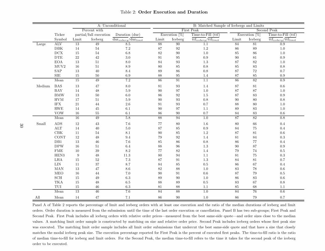
Table 2: Order Execution and Duration

A: Unconditional B: Matched Sample of Icebergs and LimitsPercent with First Peak Second Peak

Ticker partial/full execution Duration (dur) Execution [%] Time-to-Fill (ttf) Execution [%] Time-to-Fill (ttf)

Symbol Limit Iceberg duriceberg/durlimit Limit Iceberg ttficeberg/ttflimit Limit Iceberg ttficeberg/ttflimit

Large ALV 13 49 8.5 88 90 1.1 84 81 0.9DBK 14 54 7.2 87 92 1.2 86 89 1.0DCX 15 54 6.8 82 90 1.0 85 86 1.0DTE 22 42 3.0 91 95 0.9 90 81 0.9EOA 13 51 8.0 84 93 1.3 87 82 1.0MUV2 16 51 8.9 80 85 0.8 85 83 0.8SAP 13 40 8.4 89 86 0.8 87 72 0.7SIE 15 50 6.9 88 95 1.4 87 85 0.9

Mean 15 49 7.2 86 91 1.1 86 82 0.9

Medium BAS 13 47 8.0 81 93 1.4 87 81 0.6BAY 14 48 5.9 90 97 1.0 87 87 1.0BMW 13 50 6.0 86 92 1.5 87 83 0.9HVM 17 51 5.9 90 93 0.8 90 80 0.8IFX 21 44 2.6 91 93 0.7 88 80 1.0RWE 14 45 6.1 90 97 1.1 89 83 1.0VOW 16 55 6.1 86 90 0.7 84 83 0.6

Mean 16 49 5.8 88 94 1.0 87 82 0.8

Small ADS 12 43 7.6 77 80 1.6 80 66 0.4ALT 14 40 5.0 87 85 0.9 84 75 0.4CBK 11 54 8.1 90 85 1.2 87 81 0.6CONT 12 48 9.4 79 92 1.4 81 84 0.3DB1 13 46 7.6 85 86 0.8 86 77 0.4DPW 16 51 6.4 88 96 1.3 90 87 0.9FME 10 39 8.2 77 82 1.4 79 74 0.5HEN3 9 48 11.3 80 94 1.1 81 75 0.3LHA 15 52 7.3 87 91 1.3 84 81 0.7LIN 11 37 8.7 84 85 0.5 86 67 0.4MAN 13 47 8.6 82 88 1.0 83 78 0.6MEO 16 44 7.0 90 91 0.6 87 79 0.5SCH 15 49 6.3 89 90 1.0 86 83 0.6TKA 15 48 6.5 88 89 0.5 83 67 0.8TUI 15 46 6.3 81 88 1.1 85 68 1.1

Mean 13 46 7.6 84 88 1.0 84 76 0.6

All Mean 14 47 7.1 86 90 1.0 86 79 0.7

Panel A of Table 2 reports the percentage of limit and iceberg orders with at least one execution and the ratio of the median durations of iceberg and limit

orders. Order duration is measured from the submission until the time of the last order execution or cancellation. Panel B has two sub-groups; First Peak and

Second Peak. First Peak includes all iceberg orders with relative order prices—measured from the best same-side quote—and order sizes close to the median

values. A matching limit order sample is constructed by matching on size and relative order price. Second Peak includes iceberg orders whose first peak size

was executed. The matching limit order sample includes all limit order submissions that undercut the best same-side quote and that have a size that closely

matches the modal iceberg peak size. The execution percentage reported for First Peak is the percent of executed first peaks. The time-to-fill ratio is the ratio

of median time-to-fill for iceberg and limit orders. For the Second Peak, the median time-to-fill refers to the time it takes for the second peak of the iceberg

order to be executed.

30

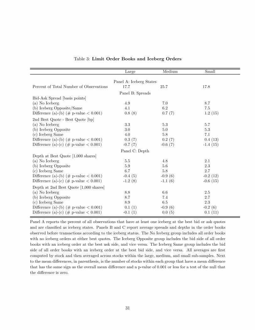
Table 3: Limit Order Books and Iceberg Orders

Large Medium Small

Panel A: Iceberg StatesPercent of Total Number of Observations 17.7 25.7 17.8

Panel B: SpreadsBid-Ask Spread [basis points](a) No Iceberg 4.9 7.0 8.7(b) Iceberg Opposite/Same 4.1 6.2 7.5Difference (a)-(b) (# p-value < 0.001) 0.8 (8) 0.7 (7) 1.2 (15)

2nd Best Quote - Best Quote [bp](a) No Iceberg 3.3 5.3 5.7(b) Iceberg Opposite 3.0 5.0 5.3(c) Iceberg Same 4.0 5.8 7.1Difference (a)-(b) (# p-value < 0.001) 0.3 (7) 0.2 (7) 0.4 (13)Difference (a)-(c) (# p-value < 0.001) -0.7 (7) -0.6 (7) -1.4 (15)

Panel C: DepthDepth at Best Quote [1,000 shares](a) No Iceberg 5.5 4.8 2.1(b) Iceberg Opposite 5.9 5.6 2.3(c) Iceberg Same 6.7 5.8 2.7Difference (a)-(b) (# p-value < 0.001) -0.4 (5) -0.9 (6) -0.2 (12)Difference (a)-(c) (# p-value < 0.001) -1.2 (8) -1.1 (6) -0.6 (15)

Depth at 2nd Best Quote [1,000 shares](a) No Iceberg 8.8 6.6 2.5(b) Iceberg Opposite 8.7 7.4 2.7(c) Iceberg Same 8.9 6.5 2.3Difference (a)-(b) (# p-value < 0.001) 0.1 (1) -0.9 (6) -0.2 (6)Difference (a)-(c) (# p-value < 0.001) -0.1 (1) 0.0 (5) 0.1 (11)

Panel A reports the percent of all observations that have at least one iceberg at the best bid or ask quotes

and are classified as iceberg states. Panels B and C report average spreads and depths in the order books

observed before transactions according to the iceberg status. The No Iceberg group includes all order books

with no iceberg orders at either best quotes. The Iceberg Opposite group includes the bid side of all order

books with an iceberg order at the best ask side, and vice versa. The Iceberg Same group includes the bid

side of all order books with an iceberg order at the best bid side, and vice versa. All averages are first

computed by stock and then averaged across stocks within the large, medium, and small sub-samples. Next

to the mean differences, in parenthesis, is the number of stocks within each group that have a mean difference

that has the same sign as the overall mean difference and a p-value of 0.001 or less for a test of the null that

the difference is zero.

31

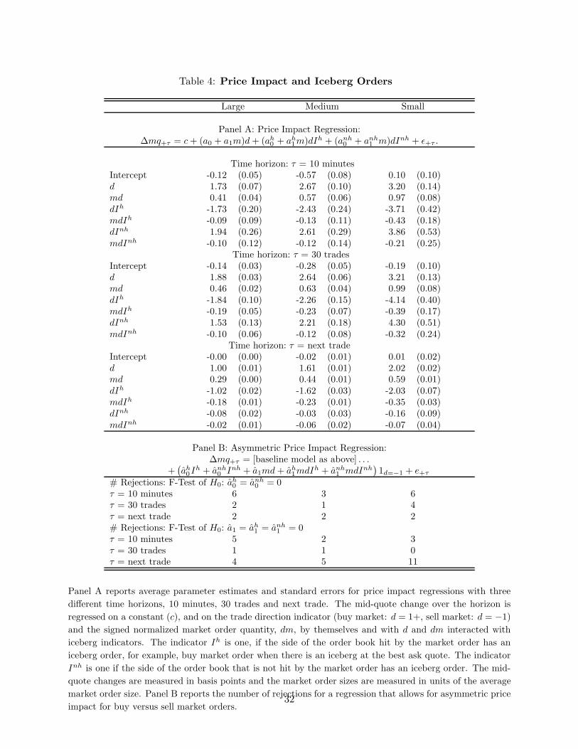
Table 4: Price Impact and Iceberg Orders

Large Medium Small

Panel A: Price Impact Regression:∆mq+τ = c + (a0 + a1m)d + (ah

0 + ah1m)dIh + (anh

0 + anh1 m)dInh + ǫ+τ .

Time horizon: τ = 10 minutesIntercept -0.12 (0.05) -0.57 (0.08) 0.10 (0.10)d 1.73 (0.07) 2.67 (0.10) 3.20 (0.14)md 0.41 (0.04) 0.57 (0.06) 0.97 (0.08)dIh -1.73 (0.20) -2.43 (0.24) -3.71 (0.42)mdIh -0.09 (0.09) -0.13 (0.11) -0.43 (0.18)dInh 1.94 (0.26) 2.61 (0.29) 3.86 (0.53)mdInh -0.10 (0.12) -0.12 (0.14) -0.21 (0.25)

Time horizon: τ = 30 tradesIntercept -0.14 (0.03) -0.28 (0.05) -0.19 (0.10)d 1.88 (0.03) 2.64 (0.06) 3.21 (0.13)md 0.46 (0.02) 0.63 (0.04) 0.99 (0.08)dIh -1.84 (0.10) -2.26 (0.15) -4.14 (0.40)mdIh -0.19 (0.05) -0.23 (0.07) -0.39 (0.17)dInh 1.53 (0.13) 2.21 (0.18) 4.30 (0.51)mdInh -0.10 (0.06) -0.12 (0.08) -0.32 (0.24)

Time horizon: τ = next tradeIntercept -0.00 (0.00) -0.02 (0.01) 0.01 (0.02)d 1.00 (0.01) 1.61 (0.01) 2.02 (0.02)md 0.29 (0.00) 0.44 (0.01) 0.59 (0.01)dIh -1.02 (0.02) -1.62 (0.03) -2.03 (0.07)mdIh -0.18 (0.01) -0.23 (0.01) -0.35 (0.03)dInh -0.08 (0.02) -0.03 (0.03) -0.16 (0.09)mdInh -0.02 (0.01) -0.06 (0.02) -0.07 (0.04)

Panel B: Asymmetric Price Impact Regression:∆mq+τ = [baseline model as above] . . .

+(

ah0Ih + anh

0 Inh + a1md + ah1mdIh + anh

1 mdInh)

1d=−1 + e+τ

# Rejections: F-Test of H0: ah0 = anh

0 = 0τ = 10 minutes 6 3 6τ = 30 trades 2 1 4τ = next trade 2 2 2# Rejections: F-Test of H0: a1 = ah

1 = anh1 = 0

τ = 10 minutes 5 2 3τ = 30 trades 1 1 0τ = next trade 4 5 11

Panel A reports average parameter estimates and standard errors for price impact regressions with three

different time horizons, 10 minutes, 30 trades and next trade. The mid-quote change over the horizon is

regressed on a constant (c), and on the trade direction indicator (buy market: d = 1+, sell market: d = −1)

and the signed normalized market order quantity, dm, by themselves and with d and dm interacted with

iceberg indicators. The indicator Ih is one, if the side of the order book hit by the market order has an

iceberg order, for example, buy market order when there is an iceberg at the best ask quote. The indicator

Inh is one if the side of the order book that is not hit by the market order has an iceberg order. The mid-

quote changes are measured in basis points and the market order sizes are measured in units of the average

market order size. Panel B reports the number of rejections for a regression that allows for asymmetric price

impact for buy versus sell market orders.32

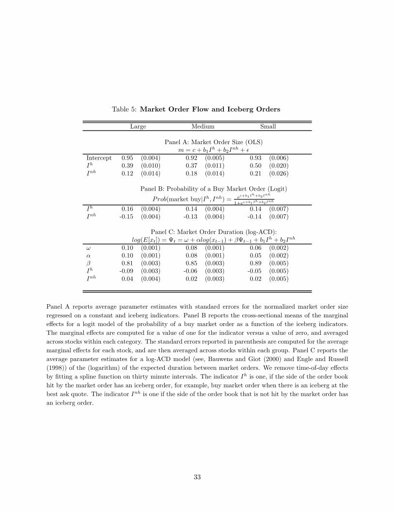
Table 5: Market Order Flow and Iceberg Orders

Large Medium Small

Panel A: Market Order Size (OLS)m = c + b1I

h + b2Inh + ǫ

Intercept 0.95 (0.004) 0.92 (0.005) 0.93 (0.006)Ih 0.39 (0.010) 0.37 (0.011) 0.50 (0.020)Inh 0.12 (0.014) 0.18 (0.014) 0.21 (0.026)

Panel B: Probability of a Buy Market Order (Logit)

Prob(market buy|Ih, Inh) = ec+b1Ih+b2I

nh

1+ec+b1Ih+b2Inh

Ih 0.16 (0.004) 0.14 (0.004) 0.14 (0.007)Inh -0.15 (0.004) -0.13 (0.004) -0.14 (0.007)

Panel C: Market Order Duration (log-ACD):log(E[xt]) = Ψt = ω + αlog(xt−1) + βΨt−1 + b1I

h + b2Inh

ω 0.10 (0.001) 0.08 (0.001) 0.06 (0.002)α 0.10 (0.001) 0.08 (0.001) 0.05 (0.002)β 0.81 (0.003) 0.85 (0.003) 0.89 (0.005)Ih -0.09 (0.003) -0.06 (0.003) -0.05 (0.005)Inh 0.04 (0.004) 0.02 (0.003) 0.02 (0.005)

Panel A reports average parameter estimates with standard errors for the normalized market order size

regressed on a constant and iceberg indicators. Panel B reports the cross-sectional means of the marginal

effects for a logit model of the probability of a buy market order as a function of the iceberg indicators.

The marginal effects are computed for a value of one for the indicator versus a value of zero, and averaged

across stocks within each category. The standard errors reported in parenthesis are computed for the average

marginal effects for each stock, and are then averaged across stocks within each group. Panel C reports the

average parameter estimates for a log-ACD model (see, Bauwens and Giot (2000) and Engle and Russell

(1998)) of the (logarithm) of the expected duration between market orders. We remove time-of-day effects

by fitting a spline function on thirty minute intervals. The indicator Ih is one, if the side of the order book

hit by the market order has an iceberg order, for example, buy market order when there is an iceberg at the

best ask quote. The indicator Inh is one if the side of the order book that is not hit by the market order has

an iceberg order.

33

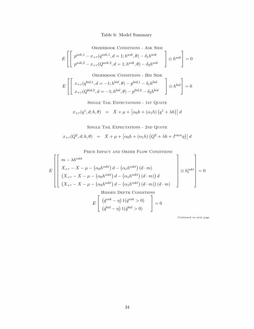
Table 6: Model Summary

Orderbook Conditions - Ask Side

E

pask,1 − x+τ (qask,1, d = 1;hask, θ) − δ1h

ask

pask,2 − x+τ (Qask,2, d = 1;hask, θ) − δ2h

ask

⊗ hask

= 0

Orderbook Conditions - Bid Side

E

x+τ (qbid,1, d = −1;hbid, θ) − pbid,1 − δ1h

bid

x+τ (Qbid,2, d = −1;hbid, θ) − pbid,2 − δ2h

bid

⊗ hbid

= 0

Single Tail Expectations - 1st Quote

x+τ (q1, d;h, θ) = X + µ +

[

α0h + (α1h)(

q1 + λh)]

d

Single Tail Expectations - 2nd Quote

x+τ (Q2, d;h, θ) = X + µ +

[

α0h + (α1h)(

Q2 + λh + Iownη)]

d

Price Impact and Order Flow Conditions

E

m − λhmkt

X+τ − X − µ −(

α0hmkt

)

d −(

α1hmkt

)

(d · m)(

X+τ − X − µ −(

α0hmkt

)

d −(

α1hmkt

)

(d · m))

d(

X+τ − X − µ −(

α0hmkt

)

d −(

α1hmkt

)

(d · m))

(d · m)

⊗ hmktt

= 0

Hidden Depth Conditions

E

(

qask − η)

1(qask > 0)(

qbid − η)

1(qbid > 0)

= 0

Continued on next page

34

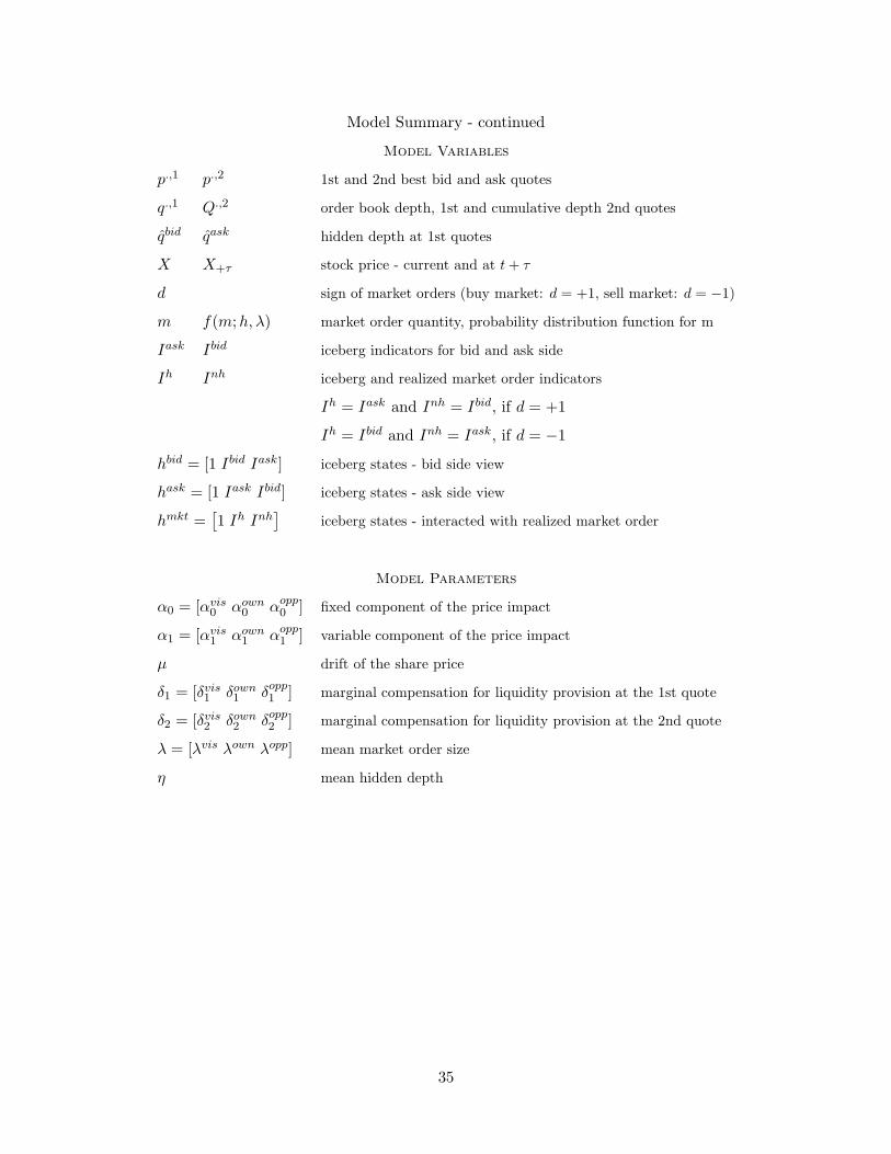
Model Summary - continued

Model Variables

p.,1 p.,2 1st and 2nd best bid and ask quotes

q.,1 Q.,2 order book depth, 1st and cumulative depth 2nd quotes

qbid qask hidden depth at 1st quotes

X X+τ stock price - current and at t + τ

d sign of market orders (buy market: d = +1, sell market: d = −1)

m f(m;h, λ) market order quantity, probability distribution function for m

Iask Ibid iceberg indicators for bid and ask side

Ih Inh iceberg and realized market order indicators

Ih = Iask and Inh = Ibid, if d = +1

Ih = Ibid and Inh = Iask, if d = −1

hbid = [1 Ibid Iask] iceberg states - bid side view

hask = [1 Iask Ibid] iceberg states - ask side view

hmkt =[

1 Ih Inh]

iceberg states - interacted with realized market order

Model Parameters

α0 = [αvis0 αown

0 αopp0

] fixed component of the price impact

α1 = [αvis1 αown

1 αopp1

] variable component of the price impact

µ drift of the share price

δ1 = [δvis1 δown

1 δopp1

] marginal compensation for liquidity provision at the 1st quote

δ2 = [δvis2 δown

2 δopp2

] marginal compensation for liquidity provision at the 2nd quote

λ = [λvis λown λopp] mean market order size

η mean hidden depth

35

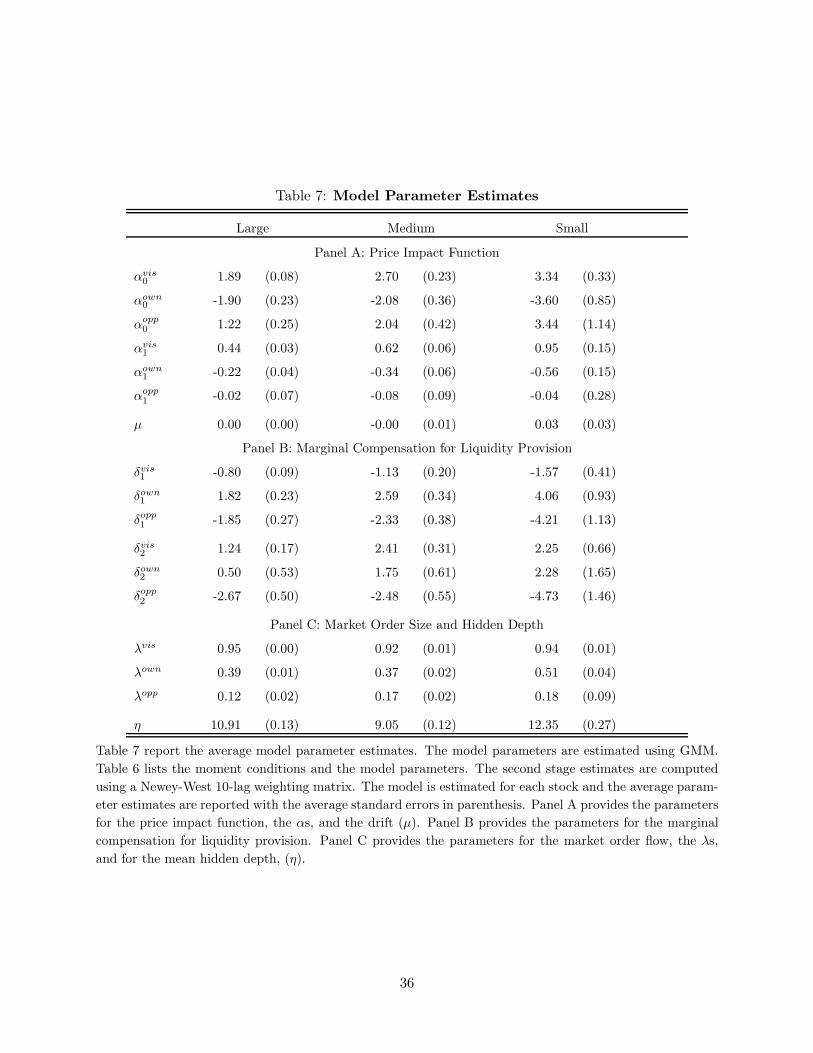
Table 7: Model Parameter Estimates

Large Medium Small

Panel A: Price Impact Function

αvis0 1.89 (0.08) 2.70 (0.23) 3.34 (0.33)

αown0 -1.90 (0.23) -2.08 (0.36) -3.60 (0.85)

αopp0 1.22 (0.25) 2.04 (0.42) 3.44 (1.14)

αvis1 0.44 (0.03) 0.62 (0.06) 0.95 (0.15)

αown1 -0.22 (0.04) -0.34 (0.06) -0.56 (0.15)

αopp1

-0.02 (0.07) -0.08 (0.09) -0.04 (0.28)

µ 0.00 (0.00) -0.00 (0.01) 0.03 (0.03)

Panel B: Marginal Compensation for Liquidity Provision

δvis1 -0.80 (0.09) -1.13 (0.20) -1.57 (0.41)

δown1 1.82 (0.23) 2.59 (0.34) 4.06 (0.93)

δopp1 -1.85 (0.27) -2.33 (0.38) -4.21 (1.13)

δvis2 1.24 (0.17) 2.41 (0.31) 2.25 (0.66)

δown2 0.50 (0.53) 1.75 (0.61) 2.28 (1.65)

δopp2 -2.67 (0.50) -2.48 (0.55) -4.73 (1.46)

Panel C: Market Order Size and Hidden Depth

λvis 0.95 (0.00) 0.92 (0.01) 0.94 (0.01)

λown 0.39 (0.01) 0.37 (0.02) 0.51 (0.04)

λopp 0.12 (0.02) 0.17 (0.02) 0.18 (0.09)

η 10.91 (0.13) 9.05 (0.12) 12.35 (0.27)

Table 7 report the average model parameter estimates. The model parameters are estimated using GMM.

Table 6 lists the moment conditions and the model parameters. The second stage estimates are computed

using a Newey-West 10-lag weighting matrix. The model is estimated for each stock and the average param-

eter estimates are reported with the average standard errors in parenthesis. Panel A provides the parameters

for the price impact function, the αs, and the drift (µ). Panel B provides the parameters for the marginal

compensation for liquidity provision. Panel C provides the parameters for the market order flow, the λs,

and for the mean hidden depth, (η).

36

Table 8: Marginal Compensation for Liquidity Provision

Large Medium Small

Mean + − Mean + − Mean + −

Best Quote Level

δvis1 -0.80 0 8 -1.13 0 5 -1.57 0 13

δvis1 + δown

1 1.02 8 0 1.46 7 0 2.48 9 0

δvis1 + δ

opp1 -2.66 0 8 -3.46 0 7 -5.79 0 14

δvis1 + δown

1 + δopp1

-0.83 0 4 -0.87 0 4 -1.73 0 7

Second Best Quote Level

δvis2 1.24 8 0 2.41 7 0 2.25 11 0

δvis2 + δown

2 1.73 6 0 4.15 6 0 4.53 9 0

δvis2 + δ

opp2 -1.43 0 3 -0.07 2 1 -2.48 1 5

δvis2 + δown

2 + δopp2 -0.94 2 1 1.68 2 0 -0.20 1 0

Table 8 reports the mean values of the net marginal compensation for liquidity provision in different states

of the order book; no iceberg orders, iceberg order on the same side as the marginal limit (own), iceberg

order on the opposite side (opp), and iceberg orders on both sides (own+opp). The units are basis points.

The marginal compensation is measured in basis points. The mean value of the estimated parameter values

or sums of parameter values are reported and the number of mean values that are significantly different from

zero at the 1% level are reported separately for positive and negative values in the columns labeled “+” and

“−.”

37

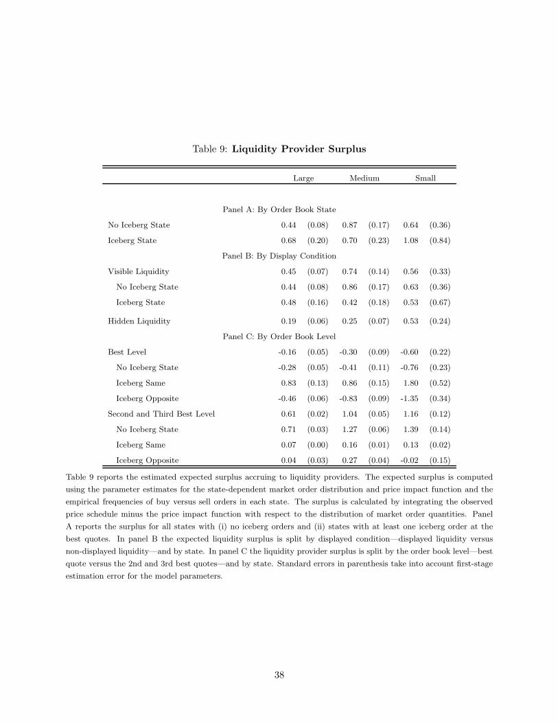
Table 9: Liquidity Provider Surplus

Large Medium Small

Panel A: By Order Book State

No Iceberg State 0.44 (0.08) 0.87 (0.17) 0.64 (0.36)

Iceberg State 0.68 (0.20) 0.70 (0.23) 1.08 (0.84)

Panel B: By Display Condition

Visible Liquidity 0.45 (0.07) 0.74 (0.14) 0.56 (0.33)

No Iceberg State 0.44 (0.08) 0.86 (0.17) 0.63 (0.36)

Iceberg State 0.48 (0.16) 0.42 (0.18) 0.53 (0.67)

Hidden Liquidity 0.19 (0.06) 0.25 (0.07) 0.53 (0.24)

Panel C: By Order Book Level

Best Level -0.16 (0.05) -0.30 (0.09) -0.60 (0.22)

No Iceberg State -0.28 (0.05) -0.41 (0.11) -0.76 (0.23)

Iceberg Same 0.83 (0.13) 0.86 (0.15) 1.80 (0.52)

Iceberg Opposite -0.46 (0.06) -0.83 (0.09) -1.35 (0.34)

Second and Third Best Level 0.61 (0.02) 1.04 (0.05) 1.16 (0.12)

No Iceberg State 0.71 (0.03) 1.27 (0.06) 1.39 (0.14)

Iceberg Same 0.07 (0.00) 0.16 (0.01) 0.13 (0.02)

Iceberg Opposite 0.04 (0.03) 0.27 (0.04) -0.02 (0.15)

Table 9 reports the estimated expected surplus accruing to liquidity providers. The expected surplus is computed

using the parameter estimates for the state-dependent market order distribution and price impact function and the

empirical frequencies of buy versus sell orders in each state. The surplus is calculated by integrating the observed

price schedule minus the price impact function with respect to the distribution of market order quantities. Panel

A reports the surplus for all states with (i) no iceberg orders and (ii) states with at least one iceberg order at the

best quotes. In panel B the expected liquidity surplus is split by displayed condition—displayed liquidity versus

non-displayed liquidity—and by state. In panel C the liquidity provider surplus is split by the order book level—best

quote versus the 2nd and 3rd best quotes—and by state. Standard errors in parenthesis take into account first-stage

estimation error for the model parameters.

38

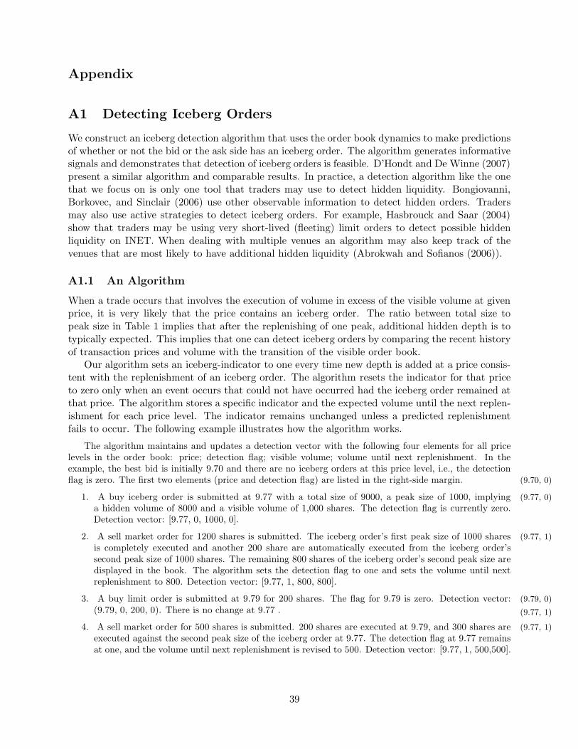
Appendix

A1 Detecting Iceberg Orders

We construct an iceberg detection algorithm that uses the order book dynamics to make predictionsof whether or not the bid or the ask side has an iceberg order. The algorithm generates informativesignals and demonstrates that detection of iceberg orders is feasible. D’Hondt and De Winne (2007)present a similar algorithm and comparable results. In practice, a detection algorithm like the onethat we focus on is only one tool that traders may use to detect hidden liquidity. Bongiovanni,Borkovec, and Sinclair (2006) use other observable information to detect hidden orders. Tradersmay also use active strategies to detect iceberg orders. For example, Hasbrouck and Saar (2004)show that traders may be using very short-lived (fleeting) limit orders to detect possible hiddenliquidity on INET. When dealing with multiple venues an algorithm may also keep track of thevenues that are most likely to have additional hidden liquidity (Abrokwah and Sofianos (2006)).

A1.1 An Algorithm

When a trade occurs that involves the execution of volume in excess of the visible volume at givenprice, it is very likely that the price contains an iceberg order. The ratio between total size topeak size in Table 1 implies that after the replenishing of one peak, additional hidden depth is totypically expected. This implies that one can detect iceberg orders by comparing the recent historyof transaction prices and volume with the transition of the visible order book.

Our algorithm sets an iceberg-indicator to one every time new depth is added at a price consis-tent with the replenishment of an iceberg order. The algorithm resets the indicator for that priceto zero only when an event occurs that could not have occurred had the iceberg order remained atthat price. The algorithm stores a specific indicator and the expected volume until the next replen-ishment for each price level. The indicator remains unchanged unless a predicted replenishmentfails to occur. The following example illustrates how the algorithm works.

The algorithm maintains and updates a detection vector with the following four elements for all pricelevels in the order book: price; detection flag; visible volume; volume until next replenishment. In theexample, the best bid is initially 9.70 and there are no iceberg orders at this price level, i.e., the detectionflag is zero. The first two elements (price and detection flag) are listed in the right-side margin. (9.70, 0)

1. A buy iceberg order is submitted at 9.77 with a total size of 9000, a peak size of 1000, implying (9.77, 0)

a hidden volume of 8000 and a visible volume of 1,000 shares. The detection flag is currently zero.Detection vector: [9.77, 0, 1000, 0].

2. A sell market order for 1200 shares is submitted. The iceberg order’s first peak size of 1000 shares (9.77, 1)

is completely executed and another 200 share are automatically executed from the iceberg order’ssecond peak size of 1000 shares. The remaining 800 shares of the iceberg order’s second peak size aredisplayed in the book. The algorithm sets the detection flag to one and sets the volume until nextreplenishment to 800. Detection vector: [9.77, 1, 800, 800].

3. A buy limit order is submitted at 9.79 for 200 shares. The flag for 9.79 is zero. Detection vector: (9.79, 0)

(9.79, 0, 200, 0). There is no change at 9.77 . (9.77, 1)

4. A sell market order for 500 shares is submitted. 200 shares are executed at 9.79, and 300 shares are (9.77, 1)

executed against the second peak size of the iceberg order at 9.77. The detection flag at 9.77 remainsat one, and the volume until next replenishment is revised to 500. Detection vector: [9.77, 1, 500,500].

39

5. A buy limit order is submitted at 9.77 for 5000 shares. The flag at 9.77 remains at one and volume (9.77, 1)

until replenishment is unchanged because the new limit order is behind the visible 500 share of theiceberg order’s second peak size. Detection vector: [9.77, 1, 5500, 500].

6. The iceberg order at 9.77 is cancelled. The detection flag remains at one.9 Detection vector: [9.77, (9.77, 1)

1, 5000, 500].

7. A sell market order is submitted for 600 shares. The flag is reset to zero as the volume until next (9.77, 0)

replenishment is exceeded without the expected replenishment. Detection vector: [9.77, 0, 4500, 0].

A1.2 Performance

The algorithm will make both type I and type II errors. We take as the null a prediction of noiceberg orders. Table A2 reports the average frequencies of type I and II errors across the fourtrading activity groups. The average frequency of type I errors is approximately one percent. Theaverage frequency of type II errors is between three and five percent. Around a third of all icebergstates are not discovered because the iceberg order remains completely unexecuted. Our resultsare comparable to those of D’Hondt and De Winne (2007).

Of course, we cannot determine to what extent the predictions from our algorithm closelyapproximates the predictions of the market participants. Conversations with market participantssuggest that it is reasonable to assume that active participants are able to collect this type ofinformation. It may also be the case that at least some market participants apply algorithms thatgenerate even more accurate predictions. For example, we have not used information in order sizesor any other characteristics that tends to be different for iceberg orders. We have also exploredwhether there is any evidence that immediate-or-cancel orders may be used to detect iceberg ordersbut while such orders are used quite frequently the connection to iceberg states is rather weak.

A1.3 Robustness of Model Parameter Estimates

We re-estimate the model parameters using the same moment conditions as above, but by lettingthe indicators generated by the detection algorithm determine the values of the indicator variables.Table A3 provides a comparison of the δ estimates obtained in the baseline case—labeled “True”—and in the case of the detection algorithm labeled “Algorithm.” Overall, the parameter estimatesare fairly close. The price impact parameters and the order flow parameters are also fairly similarsuggestion that our main findings for the compensation for liquidity provision are robust to somedegree of uncertainty about the iceberg orders.

9In principle, the algorithm could make use of the fact that the remaining volume of 5,000 at 9.77 exactly matchesthe size of the previously submitted limit order to infer that it is very likely that the drop in the visible volume at9.77 was caused by the iceberg being cancelled. However, if the limit order in question was for 500 shares instead of5,000 shares, it would be a fifty-fifty chance that the cancellation was due to the iceberg order. Our algorithm hasnot been optimized with respect to these scenarios so it is possible that its performance could be enhanced.

40

A2 Surplus Calculation

The formulas presented in sections 4.4 and ?? are independent of the choice of the market ordersize distribution. Below we provide details about the surplus calculation given the choice of anexponential distribution.

The expected surplus, πk(q), of a liquidity provider for unit q in equation (6) is

πk(q) = Pr(d = 1;h)[

pk − X − µ − (α0h) − (α1h)(q + λh)] [

1 − e−q

λh

]

(A 1)

The aggregate expected surplus of a quote, used in equations (7) and (8), in the case of theexponential distribution is calculated by

Π = Pr(d = 1;h)(λh){[

pk − X − µ − (α0h) − (α1h)(λh)] [

e−Qsλh − e−

Qeλh

]

+ (α1h)[

Qs

(

e−Qsλh

)

− Qe

(

e−Qeλh

)]}

(A 2)

where the quote starts at Qs and ends at Qe. The two formulas above are valid for the ask side,similar equations can be derived for the bid side.

A two stage approach is applied for the standard errors of the surplus expressions. The firststage considers the uncertainty of the estimated parameters of the GMM model via the deltamethod. The second stage errors are those of the sample average used to calculate the surplusexpressions itself. The two errors are combined assuming independence. Denote S as one of thesurplus calculations, then an estimator of the variance of S σ2

S is derived by the following expression

σ2S =

∂S

∂θ′V(θ)

∂S

∂θ+ s2

S (A 3)

where V(θ) is the estimated variance matrix of the model parameters and s2S is the sampling

variance of the surplus calculation. The gradient vector of the surplus expression to the parameters∂S∂θ

is calculated numerically.

41

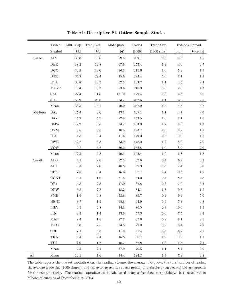
Table A1: Descriptive Statistics: Sample Stocks

Ticker Mkt. Cap Trad. Vol. Mid-Quote Trades Trade Size Bid-Ask Spread

Symbol [¿b] [¿b] [¿] [1000] [1000 shrs] [b.p.] [¿ cents]

Large ALV 33.8 18.6 99.5 289.1 0.6 4.6 4.5

DBK 38.2 19.8 67.6 253.4 1.2 4.0 2.7

DCX 30.3 12.0 36.3 211.6 1.6 5.2 1.9

DTE 34.9 22.4 15.6 284.4 5.0 7.1 1.1

EOA 33.8 10.3 52.5 183.7 1.1 4.5 2.4

MUV2 16.4 13.3 93.6 218.9 0.6 4.6 4.3

SAP 27.4 11.8 131.0 179.4 0.5 4.6 6.0

SIE 52.9 20.6 63.7 282.5 1.1 3.9 2.5

Mean 33.5 16.1 70.0 237.9 1.5 4.8 3.2

Medium BAS 25.4 8.0 43.1 165.1 1.1 4.7 2.0

BAY 15.9 5.7 22.8 153.5 1.6 7.1 1.6

BMW 12.2 5.6 34.7 134.9 1.2 5.6 1.9

HVM 6.6 6.3 18.5 123.7 2.8 9.2 1.7

IFX 4.8 9.4 11.6 179.0 4.5 10.0 1.2

RWE 12.7 6.3 33.9 148.0 1.2 5.9 2.0

VOW 9.7 6.7 39.2 162.8 1.0 5.2 2.0

Mean 12.5 6.8 29.1 152.4 1.9 6.8 1.8

Small ADS 4.1 2.0 92.5 62.6 0.4 6.7 6.1

ALT 3.3 2.0 48.8 69.9 0.6 7.4 3.6

CBK 7.6 3.4 15.3 92.7 2.4 9.6 1.5

CONT 4.1 1.6 31.5 64.0 0.8 8.8 2.8

DB1 4.8 2.3 47.0 62.8 0.8 7.0 3.3

DPW 6.8 2.8 18.2 84.1 1.8 9.3 1.7

FME 1.9 0.8 53.8 39.7 0.4 9.4 5.0

HEN3 3.7 1.2 65.8 44.9 0.4 7.3 4.8

LHA 4.5 2.8 14.1 86.5 2.3 10.6 1.5

LIN 3.4 1.4 43.6 57.3 0.6 7.5 3.3

MAN 2.4 1.8 27.7 67.6 0.9 9.1 2.5

MEO 5.0 2.5 34.8 79.0 0.9 8.4 2.9

SCH 7.1 3.3 41.0 97.4 0.8 6.7 2.7

TKA 6.4 2.4 15.8 80.7 1.9 10.7 1.7

TUI 2.0 1.7 18.7 67.8 1.3 11.5 2.1

Mean 4.5 2.1 37.9 70.5 1.1 8.7 3.0

All Mean 14.1 7.0 44.4 134.2 1.4 7.2 2.8

The table reports the market capitalization, the trading volume, the average mid-quote, the total number of trades,

the average trade size (1000 shares), and the average relative (basis points) and absolute (euro cents) bid-ask spreads

for the sample stocks. The market capitalization is calculated using a free-float methodology. It is measured in

billions of euros as of December 31st, 2003.42

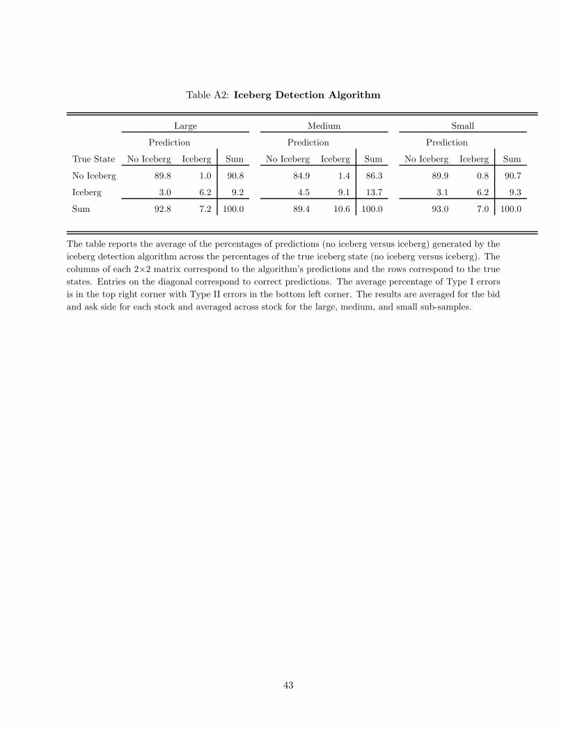
Table A2: Iceberg Detection Algorithm

Large Medium Small

Prediction Prediction Prediction

True State No Iceberg Iceberg Sum No Iceberg Iceberg Sum No Iceberg Iceberg Sum

No Iceberg 89.8 1.0 90.8 84.9 1.4 86.3 89.9 0.8 90.7

Iceberg 3.0 6.2 9.2 4.5 9.1 13.7 3.1 6.2 9.3

Sum 92.8 7.2 100.0 89.4 10.6 100.0 93.0 7.0 100.0

The table reports the average of the percentages of predictions (no iceberg versus iceberg) generated by the

iceberg detection algorithm across the percentages of the true iceberg state (no iceberg versus iceberg). The

columns of each 2×2 matrix correspond to the algorithm’s predictions and the rows correspond to the true

states. Entries on the diagonal correspond to correct predictions. The average percentage of Type I errors

is in the top right corner with Type II errors in the bottom left corner. The results are averaged for the bid

and ask side for each stock and averaged across stock for the large, medium, and small sub-samples.

43

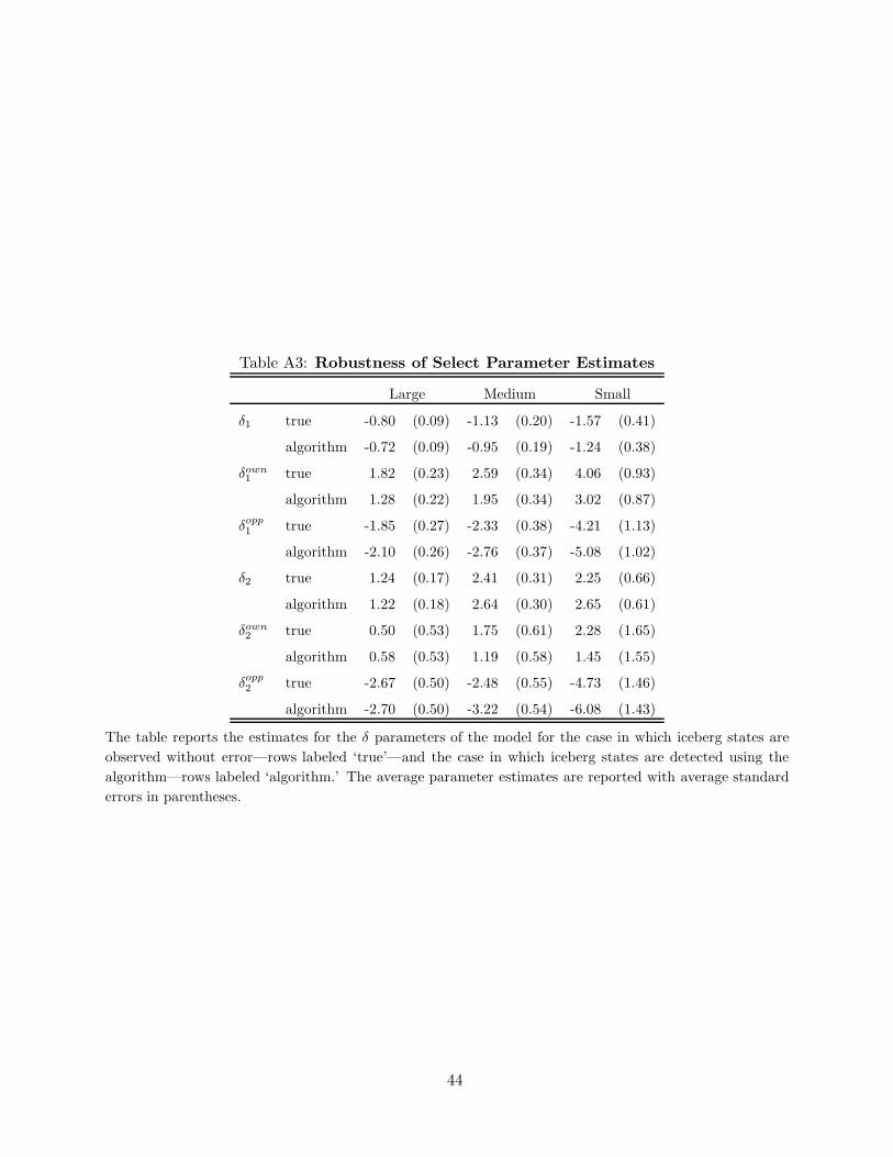
Table A3: Robustness of Select Parameter Estimates

Large Medium Small

δ1 true -0.80 (0.09) -1.13 (0.20) -1.57 (0.41)

algorithm -0.72 (0.09) -0.95 (0.19) -1.24 (0.38)

δown1 true 1.82 (0.23) 2.59 (0.34) 4.06 (0.93)

algorithm 1.28 (0.22) 1.95 (0.34) 3.02 (0.87)

δopp1 true -1.85 (0.27) -2.33 (0.38) -4.21 (1.13)

algorithm -2.10 (0.26) -2.76 (0.37) -5.08 (1.02)

δ2 true 1.24 (0.17) 2.41 (0.31) 2.25 (0.66)

algorithm 1.22 (0.18) 2.64 (0.30) 2.65 (0.61)

δown2 true 0.50 (0.53) 1.75 (0.61) 2.28 (1.65)

algorithm 0.58 (0.53) 1.19 (0.58) 1.45 (1.55)

δopp2 true -2.67 (0.50) -2.48 (0.55) -4.73 (1.46)

algorithm -2.70 (0.50) -3.22 (0.54) -6.08 (1.43)

The table reports the estimates for the δ parameters of the model for the case in which iceberg states are

observed without error—rows labeled ‘true’—and the case in which iceberg states are detected using the

algorithm—rows labeled ‘algorithm.’ The average parameter estimates are reported with average standard

errors in parentheses.

44