Optimal order placement in limit order markets - arXiv · Optimal order placement in limit order...
39
Optimal order placement in limit order markets Rama Cont and Arseniy Kukanov Imperial College London & AQR Capital Management To execute a trade, participants in electronic equity markets may choose to submit limit orders or market orders across various exchanges where a stock is traded. This decision is influenced by characteristics of the order flows and queue sizes in each limit order book, as well as the structure of transaction fees and rebates across exchanges. We propose a quantitative framework for studying this order placement problem by formulating it as a convex optimization problem. This formulation allows to study how the optimal order placement decision depends on the interplay between the state of order books, the fee structure, order flow properties and the aversion to execution risk. In the case of a single exchange, we derive an explicit solution for the optimal split between limit and market orders. For the general case of order placement across multiple exchanges, we propose a stochastic algorithm that computes the optimal routing policy and study the sensitivity of the solution to various parameters. Our solution exploits data on recent order fills across exchanges in the numerical implementation of the algorithm. Key words : limit order markets, optimal order execution, execution risk, order routing, fragmented markets, transaction costs, financial engineering, stochastic approximation, Robbins-Monro algorithm First version: October 2012. Revised: October 2014. 1 arXiv:1210.1625v4 [q-fin.TR] 23 Nov 2014
Transcript of Optimal order placement in limit order markets - arXiv · Optimal order placement in limit order...
Optimal order placement in limit order markets
Rama Cont and Arseniy KukanovImperial College London & AQR Capital Management
To execute a trade, participants in electronic equity markets may choose to submit limit orders or market
orders across various exchanges where a stock is traded. This decision is influenced by characteristics of
the order flows and queue sizes in each limit order book, as well as the structure of transaction fees and
rebates across exchanges. We propose a quantitative framework for studying this order placement problem
by formulating it as a convex optimization problem. This formulation allows to study how the optimal
order placement decision depends on the interplay between the state of order books, the fee structure, order
flow properties and the aversion to execution risk. In the case of a single exchange, we derive an explicit
solution for the optimal split between limit and market orders. For the general case of order placement across
multiple exchanges, we propose a stochastic algorithm that computes the optimal routing policy and study
the sensitivity of the solution to various parameters. Our solution exploits data on recent order fills across
exchanges in the numerical implementation of the algorithm.
Key words : limit order markets, optimal order execution, execution risk, order routing, fragmented
markets, transaction costs, financial engineering, stochastic approximation, Robbins-Monro algorithm
First version: October 2012. Revised: October 2014.
1
arX
iv:1
210.
1625
v4 [
q-fi
n.T
R]
23
Nov
201
4
R Cont and A Kukanov: Optimal order placement and routing in limit order markets2
1. Introduction
The trading process in today’s automated financial markets can be divided into several stages,
each taking place on a different time horizon: portfolio allocation decisions are made over a time
scales of weeks or days and translate into trades that are executed over time intervals of several
minutes to several days through streams of orders placed at high frequency, sometimes thousands
in a single minute (Cont 2011). Existing studies on optimal trade execution have investigated how
the execution cost of a large trade may be reduced by splitting it into multiple orders spread in
time. Once this order scheduling decision is made, one still needs to specify how each individual
order should be placed: this order placement decision involves the choice of an order type (limit
order or market order), order size and destination, when multiple trading venues are available. For
example, in the U.S. equity market there are more than ten active exchanges where a trader can
buy or sell the same securities. Order placement in a fragmented market is a non-trivial task and
brokers offer their clients smart order routing systems in addition to (and often separately from)
their suite of trade execution algorithms. We focus here on this order placement problem: given an
order which has been scheduled, choosing an order type –market or limit order– and which trading
venue(s) to submit it to.
Brokers and other active market participants need to make order placement and order routing
decisions repeatedly, thousands of times a day, and their outcomes have a significant impact on each
participant’s transaction cost. An empirical study of proprietary order data from a large execution
broker by Battalio et al. (2013) demonstrates that brokers use both limit and marketable orders
to execute trades, and the distribution of their orders across trading venues points to strategic
routing behavior. Order execution quality is materially affected by order routing choices which
recently motivated a number of inquiries by regulators into brokers’ ability to optimally place orders
on behalf of their clients (U.S. Senate 2014, Lynch and Flitter 2014, Phillips 2014). The choice
between limit and market orders and their routing is important for most market participants, not
just brokers. For instance, high-frequency traders can opportunistically provide liquidity with limit
orders or demand it with marketable orders and a large group of “mixed” high-frequency strategies
indeed relies on both order types in various proportions (see Baron et al. (2014), Brogaard et al.
(2014)). At the same time market-makers that simultaneously provide liquidity on multiple trading
venues (see Menkveld (2013)) need to take into account the fee and rebate structure and the
current state of limit order books at these venues. In aggregate, strategic order placement and
routing choices made by a variety of traders shape order flow dynamics in a fragmented market.
Boehmer and Jennings (2007) find evidence that marketable orders are sent to trading venues that
provide lower execution costs and Foucault and Menkveld (2008) show that trading fees and the
R Cont and A Kukanov: Optimal order placement and routing in limit order markets3
number of available venues affect consolidated market depth. In Moallemi et al. (2012) market
orders gravitate towards exchanges with larger posted quote sizes and low fees, while limit orders
are submitted to exchanges with high rebates and lower execution waiting times. The importance
of order placement and routing decisions on trading performance of individual market participants
justifies a more detailed modeling of order placement and routing decisions.
1.1. Literature review
Theoretical studies of limit order markets have previously considered the choice of market/limit
order type and execution venue using stylized models of trader behavior. In Foucault (1999),
Foucault et al. (2005), Rosu (2009) traders can submit one limit or market order for one trading
unit to a single exchange. There are no order queues and bid-ask spreads are determined in a
competitive equilibrium. The choice between a limit and a market order by each trader depends
on his exogenous patience parameter and the spread that he observes upon arrival. In Parlour
(1998) traders choose to place a single-unit limit or market order based on their patience and
a probability of limit order execution. There is a single exchange and traders form queues at
exogenously given bid/ask prices. Foucault and Menkveld (2008) present a model where limit order
traders form queues at two exchanges based on a profit break-even condition and then a broker can
choose to send market orders to one or both venues. These models describe market dynamics and
trader behavior in equilibrium, but require strong simplifying assumptions regarding each trader’s
order placement and routing behavior. Our analysis complements existing literature by studying
the order placement decision itself and providing insights into its structure. For instance, most
theoretical models assume that market participants need to execute one trading lot, whereas in
practice traders often need to place larger orders (e.g. the average limit order size in the U.S.
equity market is close to 400 shares). We find that the size of an order to be placed is actually
one of the most interesting input variables. It largely determines the optimal mix of market and
limit orders as well as traders’ sensitivity to exchange fees and rebates. Stylized models of trader
behavior that previously appeared in theoretical literature translate into simple, binary choices of
order type and venue based on one or two variables (e.g. bid-ask spread and trader patience). Our
analysis shows that order placement and routing decisions are more complex and need to be based
on a variety of factors. Comparing the performance of our optimal order placement strategy to
simpler rules-of-thumb for a range of parameters we find that simple heuristics are too inflexible
and often result in large transaction costs. This further motivates a need for a detailed analysis of
order placement and routing decisions, but there are few studies dedicated to this topic.
A reduced-form model for routing an infinitesimal limit order to one destination is presented in
Moallemi et al. (2012), Almgren and Harts (2008) propose a market order routing algorithm in
R Cont and A Kukanov: Optimal order placement and routing in limit order markets4
presence of hidden liquidity, while Ganchev et al. (2010) and Laruelle et al. (2011) propose numer-
ical algorithms to optimize order executions across multiple dark pools, where supply/demand is
unobserved. To the best of our knowledge this work is the first to provide a detailed treatment of
trader’s order placement decision in a multi-exchange market.
Our results also complement the literature on optimal trade execution. Early work on this subject
(Bertsimas and Lo 1998, Almgren and Chriss 2000) focused on the scheduling of orders in time
but did not explicitly model the process whereby each order is filled. More recent formulations
have tried to incorporate some elements in this direction. In one stream of literature (Obizhaeva
and Wang 2012, Alfonsi et al. 2010, Predoiu et al. 2011) traders are restricted to using only
market orders whose execution costs are given by an idealized order book shape function. Another
approach has been to model the process through which an order is filled as a dynamic random
process (Cont 2011, Cont and De Larrard 2013) leading to a formulation of the optimal execution
problem as a stochastic control problem. This formulation has been studied in various settings with
limit orders (Bayraktar and Ludkovski 2011, Gueant and Lehalle 2014) or limit and market orders
(Guilbaud and Pham 2014, Huitema 2012, Guo et al. 2013, Li 2013) but its complexity makes
it computationally intractable unless restrictive assumptions are made on price and order book
dynamics. For example, these studies commonly assume that a trader places a single limit order
for one unit at a time and its execution probability is given by a simplified function of distance
to best quotes. In our formulation limit order fills are based on order quantity, queue position and
order flows generated by other traders, as they are in actual limit order books. Existing approaches
to optimal trade execution do not consider the option of simultaneously placing limit orders on
multiple exchanges, the queue position of individual orders and the possibility of receiving partial
fills, all of which play a central role in our model.
1.2. Summary of contributions
In the present work, we adopt a more tractable approach which is closer to order routing methods
used in practice, by separating the order placement decision from the scheduling decision: assuming
that the trade execution schedule has been specified, we focus on the task of filling the scheduled
batch of orders (a trade “slice”) by optimally distributing it across trading venues and order types.
Decoupling the scheduling problem from the order placement problem is closer to market practice
(see e.g. Almgren and Harts (2008)) and leads to a more tractable approach allowing us to incorpo-
rate some realistic features which matter for order placement decisions, while conserving analytical
tractability. Although simultaneous optimization of order timing, type and routing decisions is an
interesting problem, it also appears to be intractable and its solution would likely omit details that
are important for either order placement or scheduling.
R Cont and A Kukanov: Optimal order placement and routing in limit order markets5
Our key contribution is a quantitative formulation of the order placement problem which illus-
trates how various factors - the size of an order to be placed, lengths of order queues across
exchanges, statistical properties of order flows in these exchanges, trader’s execution preferences,
and the structure of liquidity rebates across trading venues - blend into an optimal allocation of
limit orders and market orders across available trading venues. When only one exchange is avail-
able for execution, this order placement problem reduces to the problem of choosing an optimal
split between market orders and limit orders. We derive an explicit solution for this problem and
analyze its sensitivity to the order size, the trader’s urgency for filling the order and other factors.
In a case of multiple exchanges we also derive a characterization of the optimal order allocation
across trading venues. Finally, we propose a fast and flexible numerical method for solving the
order placement problem in a general case and demonstrate its efficiency through examples.
An important aspect of our framework is to account for execution risk, i.e. the risk of not filling
an order. Previous studies focus on the risk of price variations over the course of a trade execution
Almgren and Chriss (2000), Huberman and Stanzl (2005) but assume that orders are always filled.
However execution risk is a major concern for strategies that involve limit orders (Harris and
Hasbrouck 1996). When it is costly to catch up on the unfilled portion of the order, we find that
the optimal allocation shifts from limit to market orders. Although market orders are executed
at a less favorable price, it becomes optimal to use them when the execution risk is a primary
concern - for example when execution is subject to a deadline or when traders have time-sensitive
information about returns.
Optimal limit order sizes are strongly influenced by queue position that they can achieve at each
exchange and by distributions of order outflows from these queues. For example, if the queue size
at one of the exchanges is much smaller than the expected future order outflow there, it is optimal
to place a larger limit order on that exchange. Moallemi et al. (2012) argue that such favorable
limit order placement opportunities vanish in equilibrium due to competition and strategic order
routing of individual traders. However their empirical results also show that short-term deviations
from the equilibrium are a norm, and can therefore be exploited in our optimization framework.
Our order placement model brings new insights into the structure of order placement decisions.
We find that the targeted execution size plays an important role due to a bounded execution capacity
of limit orders. Relatively small quantities can be executed with a high probability using limit orders
placed just at the cheapest exchange. Faced with progressively larger quantities a trader realizes
that filling the entire amount with a single order at the cheapest exchange is unlikely and is forced
to place orders on more expensive venues. Interestingly, for relatively large quantities the optimal
order allocation becomes practically insensitive to rebates as the non-execution risk outweighs the
cost of placing limit orders on more expensive exchanges. To fill even larger quantities a trader
R Cont and A Kukanov: Optimal order placement and routing in limit order markets6
needs to start using market orders. After some point the optimal market order size increases linearly
with the targeted execution quantity while limit order sizes remain bounded at a certain value. As
a result of this feature, a larger fraction of the targeted quantity is executed with market orders
when that quantity is relatively large.
Another important aspect that appears in our analysis is the tendency of an optimal order
allocation to place more orders than it needs to fill. This overbooking behavior is due to the
possibility of receiving partial fills and the availability of multiple exchanges in our model. Instead
of placing one big limit order, a trader can place more orders to all available venues, collect
their fills and cancel the excess orders afterwards. This results in a reduction of non-execution
risk because limit order fills are not perfectly correlated. Since each venue adds new limit order
execution opportunities, overbooking becomes more prominent as the number of available venues
increases. This may explain the so-called “phantom liquidity” observed in the U.S. equity market,
i.e. a large amount of limit orders that are quickly canceled before market order traders can
execute against them. Assuming that market-makers and other limit order traders indeed post
multiple orders across exchanges and cancel all substitute orders once one of them is filled, these
“phantom” orders may represent rational attempts to reduce risk rather than a manipulative
practice. Further extrapolating this overbooking behavior to all limit order traders, our model
would predict an increase in consolidated depth with each additional trading venue. This intuition
is similar to Foucault and Menkveld (2008), although in their model limit orders are placed only
by profit-maximizing market-makers that would not post orders at an expensive venue. In our
model, overbooking (and thus an increase in consolidated depth) can occur despite high exchange
fees, which suggests that consolidated depth increases with the introduction of additional trading
venues, as long as these venues allow limit order traders to diversify their execution risk.
1.3. Outline
Section 2 describes our formulation of the order placement problem and presents conditions for the
existence of an optimal order placement. In Section 3.1 we derive an optimal split between market
and limit orders for a single exchange. Section 3.2 analyzes the general case of order placement on
multiple trading venues. Section 4 presents a numerical algorithm for solving the order placement
problem in a general case and studies its convergencee properties. Section 5.1 analyses the structure
of order placement decisions through comparative statics. Section 5.2 presents an application of
our method to historical tick data and Section 6 concludes.
R Cont and A Kukanov: Optimal order placement and routing in limit order markets7
2. The order placement problem
2.1. Decision variables
Consider a trader who needs to buy S shares of a stock within a short time interval [0, T ]. The
deadline T may be a fixed time horizon such as 1 minute, or a random stopping time, for instance
triggered by price changes or cumulative trading volume. The execution target S is assumed to
be relatively small - it is a slice of the daily trade that the trader expects to fill during [0, T ].
Nevertheless, this slice S is usually larger than a single trading lot because limit orders may have
to queue for execution for several seconds or even minutes. Our objective is to define a meaningful
framework in which the trader can compare alternative approaches to executing this trade slice
S, for example choose between sending a limit order to a single exchange, splitting it in some
proportion across K exchanges or using a combination of market and limit orders. We assume the
following two-step execution strategy - at time 0 the trader may submit K limit orders for Lk ≥ 0
shares to exchanges k= 1, . . . ,K and also market orders for M ≥ 0 shares.
At time T if the total executed quantity is less than S the trader also submits a market order
to execute the remaining amount. The trader’s order placement decision is thus summarized by a
vector X = (M,L1, . . . ,LK) ∈RK+1+ of order sizes. The components of X are non-negative (only
buy orders are allowed) and we assume that the trader has no other (e.g. pre-existing) orders in
the market.
2.2. Order execution
We will assume for simplicity that a market order of any size up to S can be filled immediately at
any single exchange. Thus a trader chooses the cheapest venue for his market orders.
Limit orders with quantities (L1, . . . ,LK) join queues of (Q1, . . . ,QK) orders in K limit order
books, where Qk ≥ 0. As a simplification we assume that all of these limit orders have the same
price - the highest bid price across venues, i.e. the National Best Bid. The case Qk = 0 is allowed in
our model and corresponds to placing limit orders inside the bid-ask spread at one of the venues.
Denote by (x)+ = max(x,0). Using the assumption that limit orders are not modified before
time T , we can explicitly calculate their filled amounts (full or partial) as a function of their initial
queue position and future order flow:
min(max(ξk−Qk,0),Lk) = (ξk−Qk)+− (ξk−Qk−Lk)+, k= 1, . . . ,K
where ξk is a total outflow from the front of the k-th queue. The order outflow ξk consists of
order cancelations that occurred before time T from queue positions in front of an order Lk, and
R Cont and A Kukanov: Optimal order placement and routing in limit order markets8
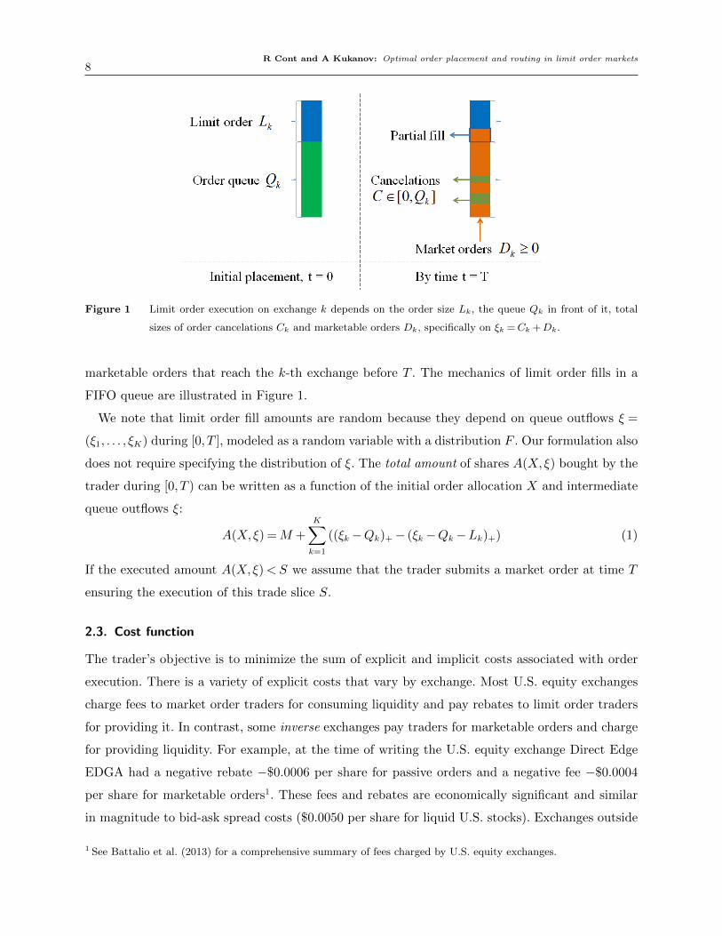
Figure 1 Limit order execution on exchange k depends on the order size Lk, the queue Qk in front of it, total
sizes of order cancelations Ck and marketable orders Dk, specifically on ξk =Ck +Dk.
marketable orders that reach the k-th exchange before T . The mechanics of limit order fills in a
FIFO queue are illustrated in Figure 1.
We note that limit order fill amounts are random because they depend on queue outflows ξ =
(ξ1, . . . , ξK) during [0, T ], modeled as a random variable with a distribution F . Our formulation also
does not require specifying the distribution of ξ. The total amount of shares A(X,ξ) bought by the
trader during [0, T ) can be written as a function of the initial order allocation X and intermediate
queue outflows ξ:
A(X,ξ) =M +K∑k=1
((ξk−Qk)+− (ξk−Qk−Lk)+) (1)
If the executed amount A(X,ξ)<S we assume that the trader submits a market order at time T
ensuring the execution of this trade slice S.
2.3. Cost function
The trader’s objective is to minimize the sum of explicit and implicit costs associated with order
execution. There is a variety of explicit costs that vary by exchange. Most U.S. equity exchanges
charge fees to market order traders for consuming liquidity and pay rebates to limit order traders
for providing it. In contrast, some inverse exchanges pay traders for marketable orders and charge
for providing liquidity. For example, at the time of writing the U.S. equity exchange Direct Edge
EDGA had a negative rebate −$0.0006 per share for passive orders and a negative fee −$0.0004
per share for marketable orders1. These fees and rebates are economically significant and similar
in magnitude to bid-ask spread costs ($0.0050 per share for liquid U.S. stocks). Exchanges outside
1 See Battalio et al. (2013) for a comprehensive summary of fees charged by U.S. equity exchanges.
R Cont and A Kukanov: Optimal order placement and routing in limit order markets9
of U.S. have adopted similar fee/rebate pricing structures (e.g. BATS Chi-X Europe), or special
rebate programs for liquidity providers (e.g. Singapore Stock Exchange, BMF-BOVESPA).
Implicit execution costs include adverse selection and market impact. Adverse selection is
reflected in the correlation between limit order executions and price changes (Glosten and Milgrom
(1985)). For example, after a buy limit order is filled prices tend to go down below its limit price
creating an immediate loss for a limit order trader. The magnitude of adverse selection losses varies
by exchange, and venues with high rebates are typically exposed to more adverse selection (see
Battalio et al. (2013)) which can be explained in a rational equilibrium model of Moallemi et al.
(2012). Small but consistent losses on limit order fills can accumulate to a significant adverse selec-
tion cost over time, which motivates us to use effective rebates rk = rek +ASk, where rek are rebates
set by exchanges and ASk are exchange-specific penalties for adverse selection. In practice these
penalties are often chosen empirically as average returns measured over a short interval following
a limit order execution.
Using the mid-quote price as a benchmark, we calculate execution costs relative to mid-quote
for an order allocation X = (M,L1, . . . ,LK) as:
(h+ f)M −K∑k=1
(h+ rk)((ξk−Qk)+− (ξk−Qk−Lk)+), (2)
where h is one-half of the bid-ask spread at time 0, f is a fee for market orders and rk are effective
rebates for limit orders on exchanges k= 1, . . . ,K.
In addition to average adverse selection losses ASk incurred on filled limit orders, a trader may
experience a shortfall due to unfilled limit orders. In the event A(X,ξ) < S the trader has to
purchase the remaining S−A(X,ξ) shares at time T with a costly market order. Adverse selection
implies that conditionally on this event prices have likely increased and the cost of market orders
at time T is higher than their cost at time 0, i.e. λu >h+ f . Alternatively, in the event A(X,ξ)>
S the prices likely decreased even more than after an average limit order fill, and λo measures
this additional adverse selection cost. To capture this execution risk we include, in the objective
function, a penalty for violations of target quantity in both directions:
λu (S−A(X,ξ))+ +λo (A(X,ξ)−S)+ , (3)
where λu ≥ 0, λo ≥ 0 are marginal penalties in dollars per share for, respectively falling behind or
exceeding the execution target S. In addition to adverse selection, the penalties λu, λo may reflect
trader’s private execution preferences. Generally, a trader can tolerate some differences between
A(X,ξ) and S because S, T are fractions of the overall trade quantity and time horizon. The
R Cont and A Kukanov: Optimal order placement and routing in limit order markets10
penalties need not be symmetric - a trader with a positive forecast of short-term returns within
the period T has a larger opportunity cost and may set λu >λo.
We also include market impact as a function of the volume of submitted orders. The target
quantity S is assumed to be small so orders (M,L1, . . . ,LK) may have little immediate impact
on prices in the interval [0, T ]. However, this impact may accumulate over the course of trading.
Accounting for average impact costs is important: it penalizes order placement strategies that
submit too many orders or orders that are too large. Empirical studies show that both market and
limit orders affect prices, and the average impact of small orders can be well approximated by a
linear function (Cont et al. (2014)), as in Kyle (1985). We assume that the impact cost is paid on
all orders placed at times 0 and T , irrespective of whether they are filled, leading to the following
total impact:
θ
(M +
K∑k=1
Lk + (S−A(X,ξ))+
), (4)
where θ > 0 is the impact coefficient.
Adding these different terms we obtain:
Definition 1 (Cost function). The cost function is defined as the sum of explicit and implicit
execution costs:
v(X,ξ) : = (h+ f)M −K∑k=1
(h+ rk) ((ξk−Qk)+− (ξk−Qk−Lk)+)
+ θ
(M +
K∑k=1
Lk + (S−A(X,ξ))+
)+λu (S−A(X,ξ)))+ +λo (A(X,ξ)−S)+ (5)
It involves the following ingredients:
• Execution objectives: target quantity S, time horizon T
• Trading costs: half of bid-ask spread h, market order fee f and effective limit order rebates
rk, market impact coefficient θ, penalties for under- and overfilling the target λu, λo
• Market configuration: number of exchanges K, limit order queues Qk.
2.4. Optimal order placement problem
We can now formulate the search for an optimal order placement as a cost minimization problem:
Problem 1 (Optimal order placement problem) An optimal order placement is a vector
X∗ ∈RK+1+ solution of
minX∈RK+1
+
V (X) (6)
R Cont and A Kukanov: Optimal order placement and routing in limit order markets11
where
V (X) =E[v(X,ξ)] =
∫RdF (dy)v(X,y) (7)
is the expected execution cost for the allocation X and the expectation is taken with respect to the
distribution F of order outflows (ξ1, ..., ξK) at horizon T .
The output is an order allocation X? = (M?,L?1, . . . ,L?K) consisting of a market order quantity M?
and limit order quantities L?1, . . . ,L?K which minimizes the expected execution cost over [0, T ].
2.5. Discussion
Before proceeding to results we discuss some of the important assumptions in our model and their
implications.
Continuous decision variables: In reality orders are integer multiples of a share; however batch
sizes are often large and one can neglect in first instance the granularity of orders and optimize
over X ∈RK+1+ , then round to number of shares in the last step. This procedure, which corresponds
to the convex relaxation of the underlying integer optimization problem (Williamson and Shmoys
2011), is indeed the standard approach used in the optimal execution literature Almgren and Chriss
(2000), Alfonsi et al. (2010), Bayraktar and Ludkovski (2011), Guilbaud and Pham (2014).
Static optimization problem: In a dynamic setting, one would need to solve Problem 1 one-step
ahead, using the conditional distribution of ξ if known:
V (tk,X∗k) = min
X∈RK+1+
E[v(X,ξt)|Ft] (8)
so insights from Problem 1 are useful for understanding the dynamic version of the problem.
Problem 1 may be seen as the stationary/ ergodic version of the problem, in which one considers
the average cost over many trades, rather than the one-step-ahead execution cost for a single
order placement. An alternative approach to order placement based on a constrained optimization
problem is discussed in the Appendix.
Execution certainty for market orders: This assumption appears to be valid as long as S is of the
same magnitude as the prevailing market depth (roughly 600 shares for an average US stock). Our
results are easily extended, at the expense of additional notation, to a case where S is large but
still can be filled with multiple market orders with progressively higher prices or fees. For example,
consider a case when there are only D1 < S shares available at the cheapest exchange with a fee
f1, but additional shares are available at a more expensive venue with a fee f2. The trader can
fill S shares by sending two market orders and their total explicit cost becomes a piece-wise linear
function of total size: f1 min(S,D1)+f2 max(S−D1,0). If S is even larger, one may add more terms
R Cont and A Kukanov: Optimal order placement and routing in limit order markets12
to this function - additional exchanges or deeper levels in the order book - by suitably increasing
their marginal costs. This generalization remains tractable as long as the cost function remains
convex (e.g. piece-wise linear). However, we note that market order routing is itself a non-trivial
problem. Practical solutions need to take into account hidden liquidity, market data speed and
trading venue geography which affects latency. These considerations are outside of the scope for
our paper that focuses primarily on limit orders and their execution in multiple order queues.
Limit order placement: We assume that limit orders L1, . . . ,LK are all placed at the same price
- the best prevailing quote. Effectively the pricing decision is narrowed to two options - a limit
order at the best quote or a marketable order. This allows us to study limit order execution in
more detail focusing on a queue of orders within a specific price level. The assumed choice appears
to be the most interesting case for applications, since in practice brokers submit the majority of
limit orders at the best bid and ask prices - see Cao et al. (2008), Battalio et al. (2013) for recent
statistics.
Exogenous spread: The spread h is exogenously set in our model, which is related our limit
order placement assumption - the trader joins an existing best quote but does not improve it.
Although this assumption appears to be restrictive from a theoretical viewpoint, in practice many
liquid assets consistently trade with a bid-ask spread equal to a single price increment, which is
exogenously set by exchanges or regulators. When the spread narrows to a single price increment,
traders cannot improve the existing quote and need to queue with their limit orders, as described
in our model.
Market impact coefficient: The coefficient θ could theoretically be different for market and limit
orders, as well as for orders sent to different exchanges. However, empirical studies show that market
impact differences between limit and market orders are small (Eisler et al. (2012), Mastromatteo
et al. (2013)). We also note that market impact occurs over time horizons that are much longer
than those involved in order placement (days as opposed to minutes or seconds), suggesting that
θ - the marginal impact of a single share - is much smaller in magnitude than bid-ask spread h
and explicit costs f, rk. For example, consider a trade to buy 5% of daily volume in a liquid stock.
Recent empirical studies (Almgren et al. 2005, Mastromatteo et al. 2013) find that the impact of
such trade is in a range of 1-6% of daily volatility, corresponding to 2-12 basis points for a stock
with 40% annualized volatility. In other words, the average change in a stock price due to this trade
is 2-12 basis points over the course of multiple hours when the trade is executed. Costs associated
with order placement decisions have similar magnitude but are incurred over much smaller time
horizons. For example, the difference between using a market order and a limit order for a U.S.
stock priced at 30 dollars per share and a spread of 1 penny can be more than 5 basis points after
accounting for liquidity fees and rebates.
R Cont and A Kukanov: Optimal order placement and routing in limit order markets13
2.6. Existence of solutions
We begin by stating certain economically reasonable restrictions on parameter values, that will be
assumed for all of our results.
A1: mink{rk} + h > 0. Interpretation: even if some effective rebates rk are negative, limit order
executions let the trader earn a fraction of the bid-ask spread.
A2: λo >h+ maxk{rk} and λo >−(h+f). Interpretation: the trader has no incentive to exceed the
target quantity S.
A3: λu >h+f . Interpretation: market orders sent at time 0 are less expensive compared to market
orders that are sent at time T conditionally on not being able to fill the target before T .
Although negative rebate values are possible, in the U.S. they are smaller than the smallest possible
value of h= $0.005, justifying our assumptions A1 and A2. Assumption A3 is motivated by adverse
selection and explained above.
Our first result, whose proof is given in the Appendix, shows that it is not optimal to submit
limit or market orders that are a priori too large or too small (larger than the target size S or
whose sum is less than S):
Proposition 1 Under assumptions A1-A3, any optimal order allocation belongs to the set:
C =
{X ∈RK+1
+
∣∣∣ 0≤M ≤ S, 0≤Lk ≤ S−M,k= 1, . . . ,K, M +K∑k=1
Lk ≥ S
}.
Proposition 1 shows that it is never optimal to overflow the target size S with a single order, but
it may be optimal to exceed the target S with the sum of order sizes M +∑K
k=1Lk. The penalty
function (3) effectively implements a soft constraint for order sizes and focuses the search for an
optimal order allocation to the set C. Specific economic or operational considerations could also
motivate adding hard constraints to problem (6), e.g. M = 0 or∑K
k=1Lk = S. Such constraints
can be easily included in our framework but absent the aforementioned considerations we do not
impose them here.
The existence of an optimal solution is then guaranteed:
Proposition 2 Under assumptions A1-A3, V : RK+1+ 7→R is convex, bounded from below and has
a global minimizer X? ∈ C.
We note that the optimal solution may be non-unique, i.e. there could be an optimal “plateau”
depending on the distribution of ξ.
R Cont and A Kukanov: Optimal order placement and routing in limit order markets14
3. Optimal order allocation
3.1. Choice of order type: limit orders vs market orders
To highlight the tradeoff between limit and market order executions in our optimization setup, we
first consider the case when the stock is traded on a single exchange, and the trader has to choose
an optimal split between limit and market orders. This special case is also economically important
because many financial assets (e.g. futures contracts, emerging market equities) in fact trade on a
single exchange.
Proposition 3 (Single exchange: optimal split between limit and market orders)
Under assumptions A1-A3:
(i) If λu ≤ λu =2h+ f + r
F (Q+S)− (h+ r+ θ), (M?,L?) = (0, S) is an optimal allocation.
(ii) If λu ≥ λu =2h+ f + r
F (Q)− (h+ r+ θ), (M?,L?) = (S,0) is an optimal allocation.
(iii) If λu ∈ (λu, λu), an optimal allocation is a mix of limit and market orders, given byM? = S−F−1
(2h+ f + r
λu +h+ r+ θ
)+Q,
L? = F−1(
2h+ f + r
λu +h+ r+ θ
)−Q,
(9)
where F (x) = P(ξ ≤ x) is the distribution of the bid queue outflows ξ and F−1 its left-inverse.
In the case of a single exchange, Proposition 1 implies that M? +L? = S, i.e. the trader does not
oversize orders. As a consequence there is no risk of exceeding the target size and λo does not
affect the optimal solution. The trader is only concerned with the risk of falling behind the target
quantity, and balances this risk with a fee, rebate and other parameters. The parameter λu is an
opportunity cost of not filling the target size, and higher values of λu lead to smaller limit order
sizes, as illustrated on Figure 2. Given that M? +L? = S, the optimal market order size increases
with an increase in λu.
The optimal split between market and limit orders depends on the distribution of outflow (execu-
tion+cancellation) through its quantile at the level 2h+f+rλu+h+r+θ
: this last formula expresses a tradeoff
between marginal costs and savings from a market order. Increasing M by 1 share immediately
increases the cost by h+ f . Since M +L= S, the trader also needs to reduce his limit order size.
This will increase the cost as the trader loses h + r in potential savings, if that limit order is
assumed to fill. However if that limit order does not fill, the trader will need to catch up paying
additional λu+ θ and not realizing any of the savings. The numerator 2h+f + r reflects costs that
the trader accepts by increasing M by 1 share, assuming his limit order will fill. The denominator
R Cont and A Kukanov: Optimal order placement and routing in limit order markets15
reflects market order benefits - if a limit order does not get a fill, the trader does not need to pay
an additional λu + θ and can forfeit h+ r in unrealized savings.
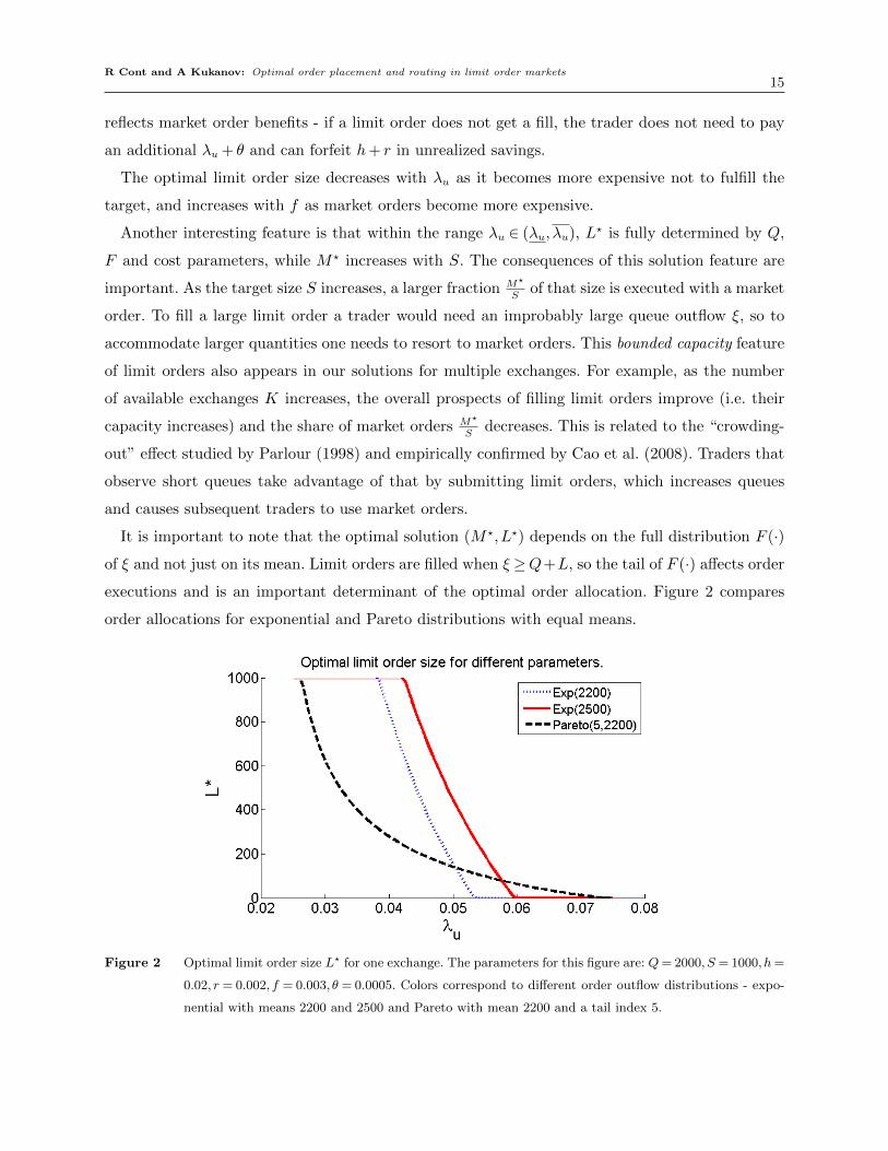
The optimal limit order size decreases with λu as it becomes more expensive not to fulfill the
target, and increases with f as market orders become more expensive.
Another interesting feature is that within the range λu ∈ (λu, λu), L? is fully determined by Q,
F and cost parameters, while M? increases with S. The consequences of this solution feature are
important. As the target size S increases, a larger fraction M?
Sof that size is executed with a market
order. To fill a large limit order a trader would need an improbably large queue outflow ξ, so to
accommodate larger quantities one needs to resort to market orders. This bounded capacity feature
of limit orders also appears in our solutions for multiple exchanges. For example, as the number
of available exchanges K increases, the overall prospects of filling limit orders improve (i.e. their
capacity increases) and the share of market orders M?
Sdecreases. This is related to the “crowding-
out” effect studied by Parlour (1998) and empirically confirmed by Cao et al. (2008). Traders that
observe short queues take advantage of that by submitting limit orders, which increases queues
and causes subsequent traders to use market orders.
It is important to note that the optimal solution (M?,L?) depends on the full distribution F (·)
of ξ and not just on its mean. Limit orders are filled when ξ ≥Q+L, so the tail of F (·) affects order
executions and is an important determinant of the optimal order allocation. Figure 2 compares
order allocations for exponential and Pareto distributions with equal means.
Figure 2 Optimal limit order size L? for one exchange. The parameters for this figure are: Q= 2000, S = 1000, h=
0.02, r = 0.002, f = 0.003, θ = 0.0005. Colors correspond to different order outflow distributions - expo-
nential with means 2200 and 2500 and Pareto with mean 2200 and a tail index 5.
R Cont and A Kukanov: Optimal order placement and routing in limit order markets16
3.2. Optimal routing of limit orders across multiple exchanges
When multiple trading venues are available, dividing a target quantity among them reduces the
risk of not filling an order and improves execution quality, and one may even consider sending S
shares to each exchange. However, sending too many orders leads to excessive market impact and
an undesirable possibility of over-trading. Proposition 4 gives optimality conditions for an order
allocation X? = (M?,L?1, . . . ,L?K):
Proposition 4 Assume A1-A3 hold, the distribution of ξ is continuous, maxk{Fk(Qk +S)} < 1
and λu <maxk
{2h+ f + rkFk(Qk)
− (h+ rk + θ)
}. Then:
1. Let p0 = P (ξ1 ≤Q1, ..., ξk ≤QK). If
λu ≥2h+ f + max
k{rk}
p0− (h+ max
k{rk})
then optimal order placement strategy involves market orders: M? > 0.
2. If cost savings and fill probability on exchange j overweigh market impact :
(h+ rj −λo)P (ξj >Qj)> θ
then any optimal order placement involves limit orders on exchange j: L?j > 0.
3. If previous assumptions hold for all exchanges j = 1, . . . ,K, X? ∈ C is an optimal allocation
if and only if
P
(M? +
K∑k=1
((ξk−Qk)+− (ξk−Qk−L?k)+)<S
)=h+ f +λo + θ
λu +λo + θ(10)
P
(M? +
K∑k=1
((ξk−Qk)+− (ξk−Qk−L?k)+)<S
∣∣∣∣ξj >Qj +L?j
)=
θP(ξj>Qj+L∗j )
+λo− (h+ rj)
λu +λo + θ,
for j = 1, . . . ,K. (11)
The optimality criterion (10)-(11) is simple - it depends on the probabilities of an execution
shortfall A(X,ξ)< S. Proposition 4 thus establishes that for X to be optimal it is necessary and
sufficient that X equates these execution shortfall probabilities to values computed with model
parameters.
When the number of exchanges K is large, shorfall probabilities in (10)-(11) are difficult to
compute in closed-form. However, the case K = 2 is relatively tractable and will be analyzed as an
illustration. The assumption of independence between ξ1, ξ2 is made only in this example and is
not required for the rest of our results. In Section 4 we present results for correlated order flows.
R Cont and A Kukanov: Optimal order placement and routing in limit order markets17
Corollary In addition to assumptions of Proposition 4, assume that K = 2 and ξ1, ξ2 are indepen-
dent. Also, assume that F1,2(Q1,2)< 1− h+ r2,1λo
and (h+ r1,2)P (ξ1,2 >Q1,2 +S)> θ. Then there is
an optimal order allocation X? = (M?,L?1,L?2)∈ int{C} and it solves the following equations
L?1 =Q2 +S−M?−F−12
(−θ/F1(Q1 +L?1) +λu + θ+h+ r1
λu +λo + θ
)(12a)
L?2 =Q1 +S−M?−F−11
(−θ/F2(Q2 +L?2) +λu + θ+h+ r2
λu +λo + θ
)(12b)
F1(Q1 +L?1)F2(Q2 +S−M?−L?1) +
Q1+L?1∫
Q1+S−M?−L?2
F2(Q1 +Q2 +S−M?−x1)dF1(x1) =λu− (h+ f)
λu +λo + θ, (12c)
where F1(·),F2(·) are the cdf functions of ξ1, ξ2 respectively and Fi = 1−Fi.
In (12a)–(12b) the optimal limit order quantities L?1,L?2 are linear functions of M?. When (12a)-
(12b) are substituted into (12c) we obtain a non-linear equation for M?, which can be solved for
M∗.
4. An optimal order routing algorithm
4.1. A stochastic algorithm based on order flow sampling
Practical applications require a fast and flexible method for optimizing order placement across
multiple trading venues. As the number of venues increases, it becomes progressively more difficult
to evaluate the objective function V (X) - a K-dimensional integral - and to obtain analytical
solutions for the order placement problem. In this section we propose a stochastic approximation
method for efficiently computing the optimal allocation even in high dimensions. The idea is to
sample order outflows ξk and approximate the gradient of V (X) along a random optimization path.
Applying this approach for our problem formulation yields an intuitive iterative algorithm that
updates trader’s order allocation in response to past order execution outcomes.
Our numerical solution is based on the robust stochastic approximation algorithm of Nemirovski
et al. (2009). Denote by g(X,ξ) =∇v(X,ξ) the gradient of v(X,ξ) with respect to X. The idea is
to use a random samples ξn ∈RK from ξ to approximate, iteratively, V (X) and its gradient:
1: Choose an initial X0 ∈RK+1 and fix a step size γ;
2: for n= 1, . . . ,N do
3: Xn =Xn−1− γg(Xn−1, ξn)
4: end
5: An estimator X∗ is given by: X?N = 1
N
∑N
n=1Xn
Here random variables ξn are assumed to be an ergodic sequence sampled from the distribution F ,
which may or may not be known. Under mild assumptions, satisfied by our objective function, the
R Cont and A Kukanov: Optimal order placement and routing in limit order markets18
estimator X?N converges to an optimal solution X? and has a performance bound
V (X?)−V (X?)≤ DM√N
, where D= maxX,X′∈C
‖X −X ′‖2, M =√
maxX∈C
E [‖g(X,ξ)‖22].
The optimal step size is γ? = D√NM
and we use a step size
γ =K1/2S
(N(h+ f + θ+λu +λo)
2 +NK∑k=1
(h+ rk + θ+λu +λo)2
)−1/2that scales appropriately with problem parameters. For more details on stochastic approximation
methods we refer to Kushner and Yin (2003) and Nemirovski et al. (2009).
In general, this method requires a sample of size N of the random variable ξ. Since g(Xn, ξ)
depends on random variables ξ only through indicator functions:
g(Xn, ξ) =
h+ f + θ− (λu + θ)1{A(Xn,ξ)<S}+λo1{A(Xn,ξ)>S}
θ+1{ξ1>Q1+L1,n}(−(h+ r1)− (λu + θ)1{A(Xn,ξ)<S}+λo1{A(Xn,ξ)>S}
). . .
θ+1{ξK>QK+LK,n}(−(h+ rK)− (λu + θ)1{A(Xn,ξ)<S}+λo1{A(Xn,ξ)>S}
)
a practical approach is to store the values of these indicator functions from past order executions
at each exchange and use them to compute the sample values ξn.
These indicators have simple interpretations: 1{A(Xn,ξ)<S} = 1 if on the n−th order submission
the trader fell behind the target quantity, 1{A(Xn,ξ)>S} = 1 if he was ahead of the target, and
1{ξk>Qk+Lk,n} = 1 if a limit order on exchange k was fully executed. This leads to a non-parametric
online implementation of the algorithm, which updates order sizes in response to previous order
execution outcomes, and can be interpreted as a sequential learning procedure. For example, the
first row of g(Xn, ξ) describes updates of the market order quantity M :
• on each iteration M is decreased by γ(h+ f + θ) to reduce trading costs and market impact
• if a trader fell behind his target quantity, M will increase by γ(λu + θ) to reduce the shortfall
on the next execution
• since overtrading is also penalized, M is decreased by γλo whenever a target quantity is
exceeded
Limit order sizes are updated similarly. If a limit order is not filled, its quantity will be reduced by
γθ to reduce market impact, otherwise the update depends on a fill outcome.
The algorithm is fast - it updates an allocation vector sequentially and each update involves
at most 5(K + 1) arithmetic operations. On a retail laptop computer, an optimal order allocation
across 12 exchanges can be computed in less than 200 milliseconds using an approximation with
N = 1000 iterations. The sequential nature of the algorithm allows to easily adapt it for low-latency
trading applications: each iteration takes a fraction of a millisecond. First, optimal allocations are
R Cont and A Kukanov: Optimal order placement and routing in limit order markets19
computed off-line and stored in a table. The table can be indexed by parameters such as Qk, S,T .
Then, an allocation is retrieved from the table in real-time, routing decisions are made and orders
are sent. Finally, order fills are collected, the allocation is updated by one iteration as described by
g, and stored in the table for future use. In Section 5.2 we present an illustration of this approach
based on historical tick data.
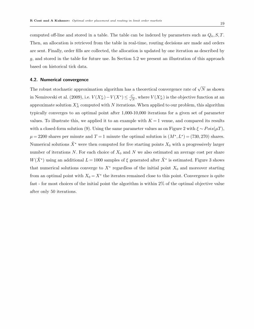
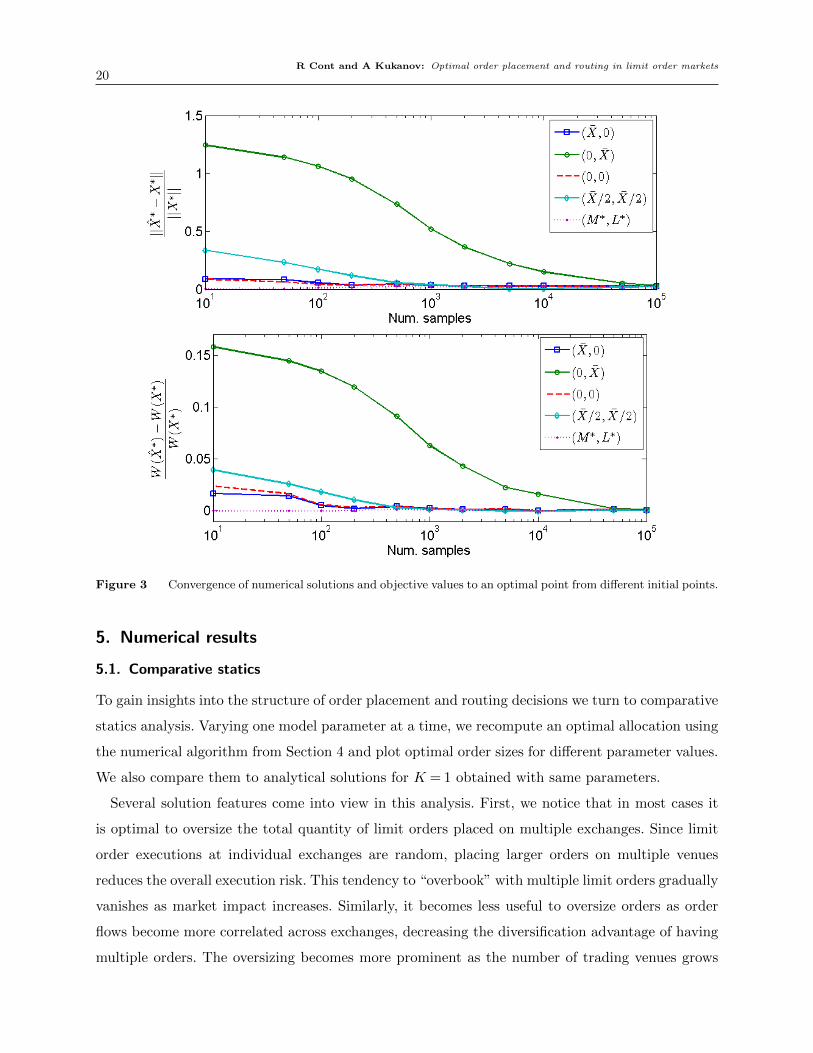
4.2. Numerical convergence
The robust stochastic approximation algorithm has a theoretical convergence rate of√N as shown
in Nemirovski et al. (2009), i.e. V (X?N)−V (X?)≤ C√
N, where V (X?
N) is the objective function at an
approximate solutionX?N computed withN iterations. When applied to our problem, this algorithm
typically converges to an optimal point after 1,000-10,000 iterations for a given set of parameter
values. To illustrate this, we applied it to an example with K = 1 venue, and compared its results
with a closed-form solution (9). Using the same parameter values as on Figure 2 with ξ ∼ Pois(µT ),
µ= 2200 shares per minute and T = 1 minute the optimal solution is (M?,L?) = (730,270) shares.
Numerical solutions X? were then computed for five starting points X0 with a progressively larger
number of iterations N . For each choice of X0 and N we also estimated an average cost per share
W (X?) using an additional L= 1000 samples of ξ generated after X? is estimated. Figure 3 shows
that numerical solutions converge to X? regardless of the initial point X0 and moreover starting
from an optimal point with X0 =X? the iterates remained close to this point. Convergence is quite
fast - for most choices of the initial point the algorithm is within 2% of the optimal objective value
after only 50 iterations.
R Cont and A Kukanov: Optimal order placement and routing in limit order markets20
Figure 3 Convergence of numerical solutions and objective values to an optimal point from different initial points.
5. Numerical results
5.1. Comparative statics
To gain insights into the structure of order placement and routing decisions we turn to comparative
statics analysis. Varying one model parameter at a time, we recompute an optimal allocation using
the numerical algorithm from Section 4 and plot optimal order sizes for different parameter values.
We also compare them to analytical solutions for K = 1 obtained with same parameters.
Several solution features come into view in this analysis. First, we notice that in most cases it
is optimal to oversize the total quantity of limit orders placed on multiple exchanges. Since limit
order executions at individual exchanges are random, placing larger orders on multiple venues
reduces the overall execution risk. This tendency to “overbook” with multiple limit orders gradually
vanishes as market impact increases. Similarly, it becomes less useful to oversize orders as order
flows become more correlated across exchanges, decreasing the diversification advantage of having
multiple orders. The oversizing becomes more prominent as the number of trading venues grows
R Cont and A Kukanov: Optimal order placement and routing in limit order markets21
leading to more opportunities to diversify limit order fills. Larger target trade sizes also lead to
more order oversizing. This suggests that large traders need to seek liquidity opportunities to fill
a large trade even at a cost of creating some market impact with their limit orders.
Second, we find that limit orders have a bounded capacity for executing large trades. The quantity
that is likely to be filled with a limit order on exchange k is given by a queue size Qk and a order
outflow distribution, more precisely by its tail P(ξk >x), x >Qk. Filling a relatively small quantity
S can usually be achieved by just placing several limit orders, but to fill larger quantities a trader
needs to rely on market orders. A number of available venues plays a role in this tradeoff - the
more venues are available, the more likely a trader can fill some of his limit orders, which makes
market orders less necessary.
Third, we show that the target quantity S itself determines which parameters drive its optimal
allocation. For smaller S, our solutions quickly shift to limit orders on venues that provide the
largest effective rebate. For larger S we see that under- and overfill penalties play a more significant
role and solutions become insensitive to rebates. Queue sizes and order outflow distributions appear
to be important in all cases.
The baseline set of parameters in our analysis is representative of a typical stock in the U.S.
equity market. We set f = 0.003, h= 0.02, θ= 0.0005, λu = λo = 0.05 and K = 2. Exchange param-
eters are set to Qk = 2000, rk = 0.002 for all venues. Order outflows follow a simple single-factor
model, capturing the fact that order flows in a fragmented market are usually positively correlated.
Specifically we put ξk = αξ0 + (1− α)εk, where ξ0, εk are i.i.d. Poisson random variables with
a common mean parameter µT , µ= 2200 shares/minute, T = 1 minute and α= 0.6. To compute
each numerical solution we used N = 1000 samples. This was enough for convergence, regardless
of the number of exchanges K as the algorithm remains largely unchanged with different K. With
the exception of a comparison across values of µ, in all other solution comparisons we used the
same samples of ξk across a range of parameter values. For analytical solutions we assumed a sim-
ple Poisson distribution for order flows with the same mean µT . Comparing solutions for K = 1
and K = 2 we find that order allocations for multiple venues are in many cases similar to their
single-venue counterparts.
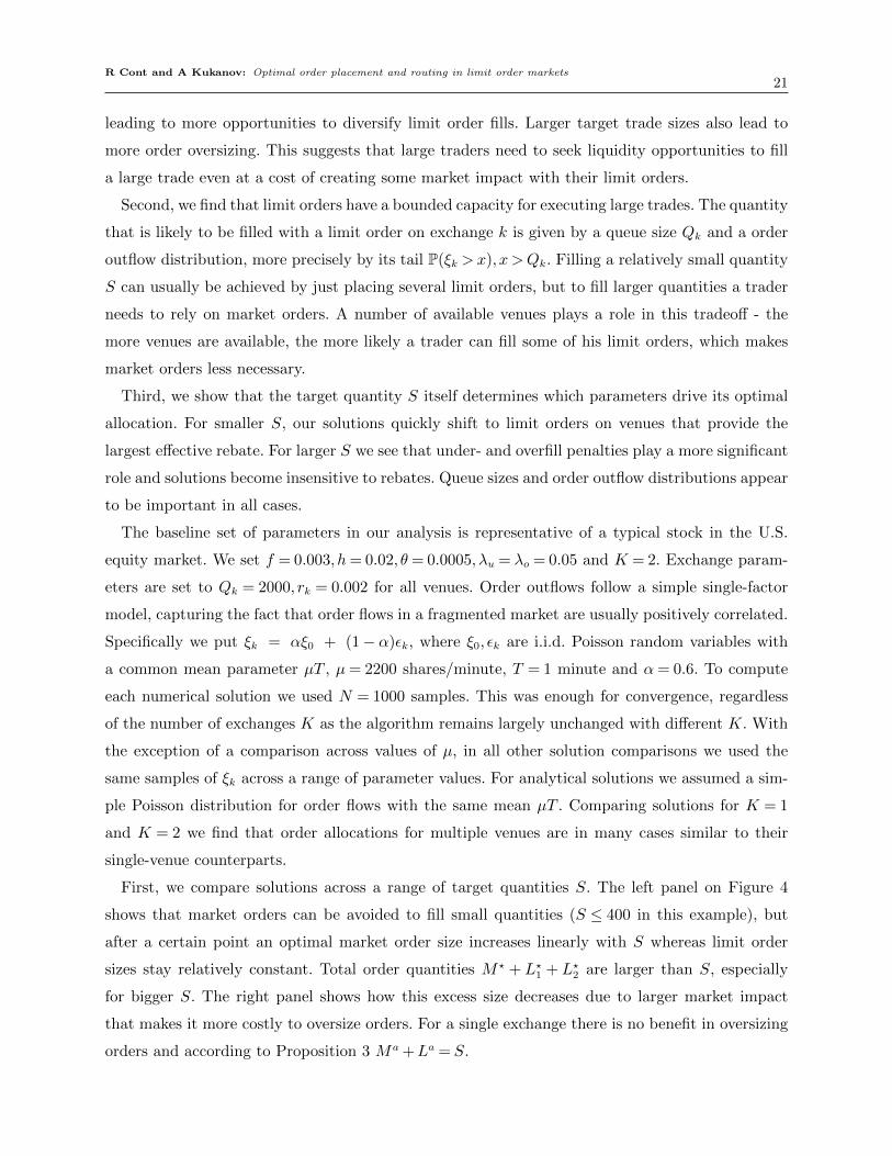
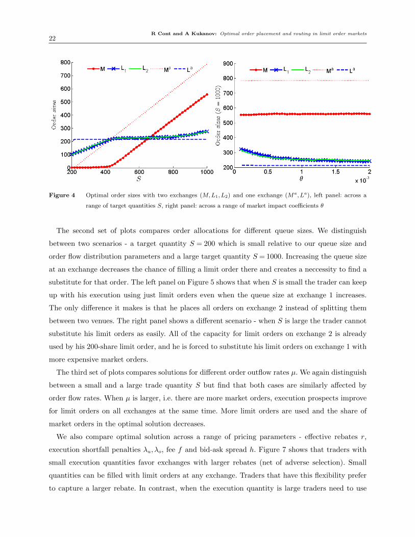
First, we compare solutions across a range of target quantities S. The left panel on Figure 4
shows that market orders can be avoided to fill small quantities (S ≤ 400 in this example), but
after a certain point an optimal market order size increases linearly with S whereas limit order
sizes stay relatively constant. Total order quantities M? + L?1 + L?2 are larger than S, especially
for bigger S. The right panel shows how this excess size decreases due to larger market impact
that makes it more costly to oversize orders. For a single exchange there is no benefit in oversizing
orders and according to Proposition 3 Ma +La = S.
R Cont and A Kukanov: Optimal order placement and routing in limit order markets22
Figure 4 Optimal order sizes with two exchanges (M,L1,L2) and one exchange (Ma,La), left panel: across a
range of target quantities S, right panel: across a range of market impact coefficients θ
The second set of plots compares order allocations for different queue sizes. We distinguish
between two scenarios - a target quantity S = 200 which is small relative to our queue size and
order flow distribution parameters and a large target quantity S = 1000. Increasing the queue size
at an exchange decreases the chance of filling a limit order there and creates a neccessity to find a
substitute for that order. The left panel on Figure 5 shows that when S is small the trader can keep
up with his execution using just limit orders even when the queue size at exchange 1 increases.
The only difference it makes is that he places all orders on exchange 2 instead of splitting them
between two venues. The right panel shows a different scenario - when S is large the trader cannot
substitute his limit orders as easily. All of the capacity for limit orders on exchange 2 is already
used by his 200-share limit order, and he is forced to substitute his limit orders on exchange 1 with
more expensive market orders.
The third set of plots compares solutions for different order outflow rates µ. We again distinguish
between a small and a large trade quantity S but find that both cases are similarly affected by
order flow rates. When µ is larger, i.e. there are more market orders, execution prospects improve
for limit orders on all exchanges at the same time. More limit orders are used and the share of
market orders in the optimal solution decreases.
We also compare optimal solution across a range of pricing parameters - effective rebates r,
execution shortfall penalties λu, λo, fee f and bid-ask spread h. Figure 7 shows that traders with
small execution quantities favor exchanges with larger rebates (net of adverse selection). Small
quantities can be filled with limit orders at any exchange. Traders that have this flexibility prefer
to capture a larger rebate. In contrast, when the execution quantity is large traders need to use
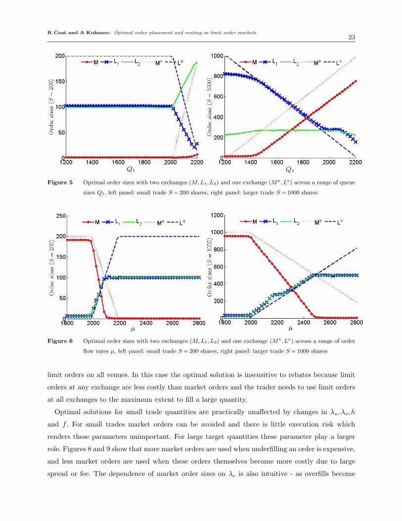
R Cont and A Kukanov: Optimal order placement and routing in limit order markets23
Figure 5 Optimal order sizes with two exchanges (M,L1,L2) and one exchange (Ma,La) across a range of queue
sizes Q1, left panel: small trade S = 200 shares, right panel: larger trade S = 1000 shares
Figure 6 Optimal order sizes with two exchanges (M,L1,L2) and one exchange (Ma,La) across a range of order
flow rates µ, left panel: small trade S = 200 shares, right panel: larger trade S = 1000 shares
limit orders on all venues. In this case the optimal solution is insensitive to rebates because limit
orders at any exchange are less costly than market orders and the trader needs to use limit orders
at all exchanges to the maximum extent to fill a large quantity.
Optimal solutions for small trade quantities are practically unaffected by changes in λu, λo, h
and f . For small trades market orders can be avoided and there is little execution risk which
renders these parameters unimportant. For large target quantities these parameter play a larger
role. Figures 8 and 9 show that more market orders are used when underfilling an order is expensive,
and less market orders are used when these orders themselves become more costly due to large
spread or fee. The dependence of market order sizes on λo is also intuitive - as overfills become
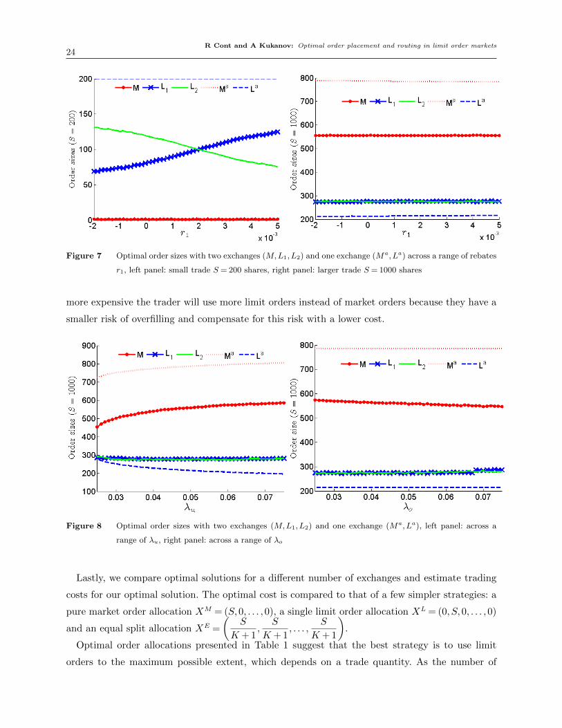
R Cont and A Kukanov: Optimal order placement and routing in limit order markets24
Figure 7 Optimal order sizes with two exchanges (M,L1,L2) and one exchange (Ma,La) across a range of rebates
r1, left panel: small trade S = 200 shares, right panel: larger trade S = 1000 shares
more expensive the trader will use more limit orders instead of market orders because they have a
smaller risk of overfilling and compensate for this risk with a lower cost.
Figure 8 Optimal order sizes with two exchanges (M,L1,L2) and one exchange (Ma,La), left panel: across a
range of λu, right panel: across a range of λo
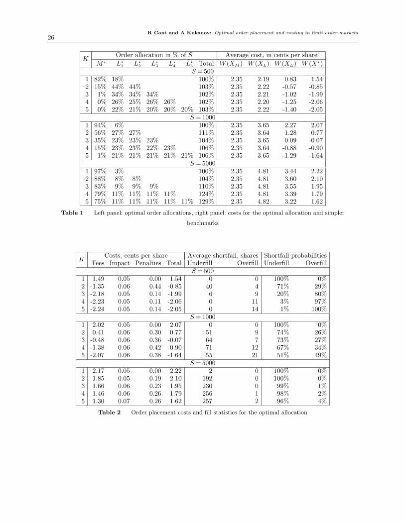
Lastly, we compare optimal solutions for a different number of exchanges and estimate trading
costs for our optimal solution. The optimal cost is compared to that of a few simpler strategies: a
pure market order allocation XM = (S,0, . . . ,0), a single limit order allocation XL = (0, S,0, . . . ,0)
and an equal split allocation XE =
(S
K + 1,
S
K + 1, . . . ,
S
K + 1
).
Optimal order allocations presented in Table 1 suggest that the best strategy is to use limit
orders to the maximum possible extent, which depends on a trade quantity. As the number of
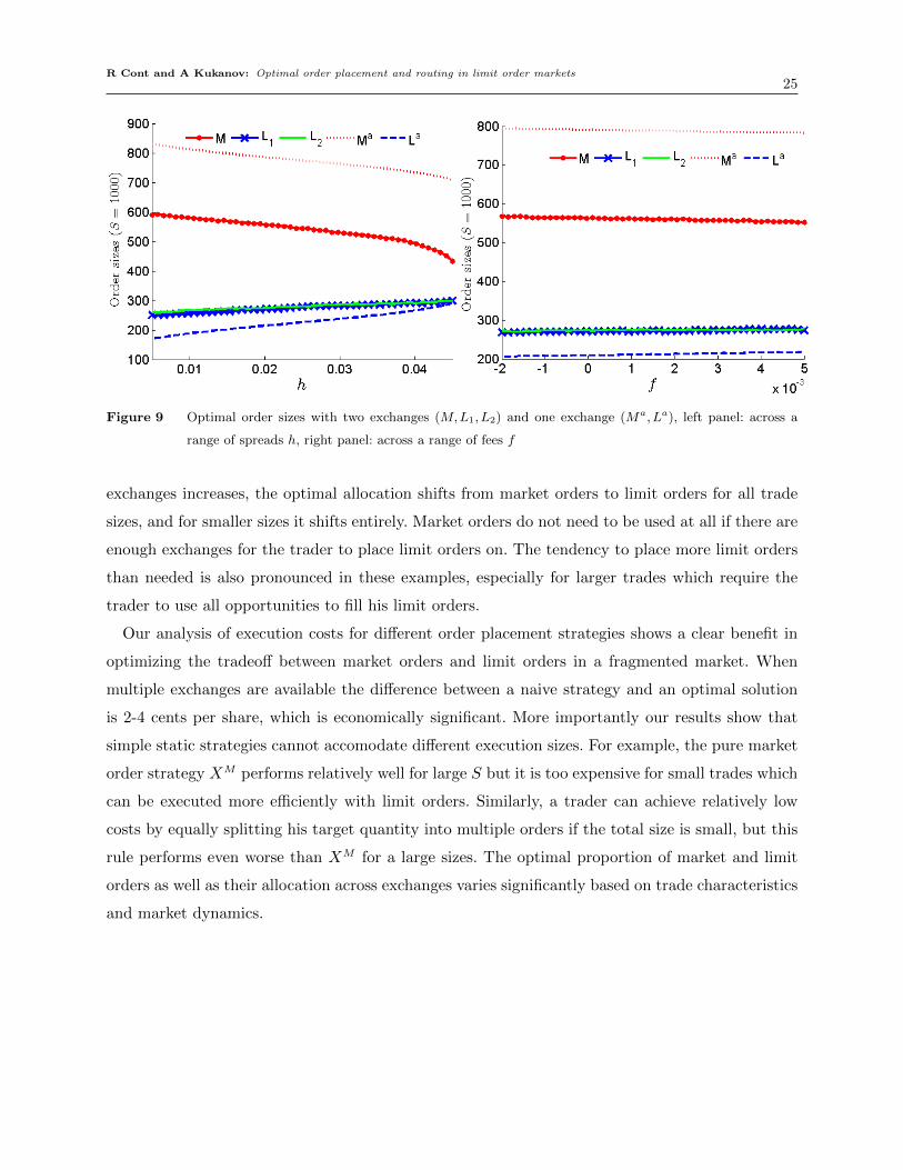
R Cont and A Kukanov: Optimal order placement and routing in limit order markets25
Figure 9 Optimal order sizes with two exchanges (M,L1,L2) and one exchange (Ma,La), left panel: across a
range of spreads h, right panel: across a range of fees f
exchanges increases, the optimal allocation shifts from market orders to limit orders for all trade
sizes, and for smaller sizes it shifts entirely. Market orders do not need to be used at all if there are
enough exchanges for the trader to place limit orders on. The tendency to place more limit orders
than needed is also pronounced in these examples, especially for larger trades which require the
trader to use all opportunities to fill his limit orders.
Our analysis of execution costs for different order placement strategies shows a clear benefit in
optimizing the tradeoff between market orders and limit orders in a fragmented market. When
multiple exchanges are available the difference between a naive strategy and an optimal solution
is 2-4 cents per share, which is economically significant. More importantly our results show that
simple static strategies cannot accomodate different execution sizes. For example, the pure market
order strategy XM performs relatively well for large S but it is too expensive for small trades which
can be executed more efficiently with limit orders. Similarly, a trader can achieve relatively low
costs by equally splitting his target quantity into multiple orders if the total size is small, but this
rule performs even worse than XM for a large sizes. The optimal proportion of market and limit
orders as well as their allocation across exchanges varies significantly based on trade characteristics
and market dynamics.
R Cont and A Kukanov: Optimal order placement and routing in limit order markets26
KOrder allocation in % of S Average cost, in cents per share
M? L?1 L?2 L?3 L?4 L?5 Total W (XM) W (XL) W (XE) W (X?)S = 500
1 82% 18% 100% 2.35 2.19 0.83 1.542 15% 44% 44% 103% 2.35 2.22 -0.57 -0.853 1% 34% 34% 34% 102% 2.35 2.21 -1.02 -1.994 0% 26% 25% 26% 26% 102% 2.35 2.20 -1.25 -2.065 0% 22% 21% 20% 20% 20% 103% 2.35 2.22 -1.40 -2.05
S = 10001 94% 6% 100% 2.35 3.65 2.27 2.072 56% 27% 27% 111% 2.35 3.64 1.28 0.773 35% 23% 23% 23% 104% 2.35 3.65 0.09 -0.074 15% 23% 23% 22% 23% 106% 2.35 3.64 -0.88 -0.905 1% 21% 21% 21% 21% 21% 106% 2.35 3.65 -1.29 -1.64
S = 50001 97% 3% 100% 2.35 4.81 3.44 2.222 88% 8% 8% 104% 2.35 4.81 3.60 2.103 83% 9% 9% 9% 110% 2.35 4.81 3.55 1.954 79% 11% 11% 11% 11% 124% 2.35 4.81 3.39 1.795 75% 11% 11% 11% 11% 11% 129% 2.35 4.82 3.22 1.62
Table 1 Left panel: optimal order allocations, right panel: costs for the optimal allocation and simpler
benchmarks
KCosts, cents per share Average shortfall, shares Shortfall probabilities
Fees Impact Penalties Total Underfill Overfill Underfill OverfillS = 500
1 1.49 0.05 0.00 1.54 0 0 100% 0%2 -1.35 0.06 0.44 -0.85 40 4 71% 29%3 -2.18 0.05 0.14 -1.99 6 9 20% 80%4 -2.23 0.05 0.11 -2.06 0 11 3% 97%5 -2.24 0.05 0.14 -2.05 0 14 1% 100%
S = 10001 2.02 0.05 0.00 2.07 0 0 100% 0%2 0.41 0.06 0.30 0.77 51 9 74% 26%3 -0.48 0.06 0.36 -0.07 64 7 73% 27%4 -1.38 0.06 0.42 -0.90 71 12 67% 34%5 -2.07 0.06 0.38 -1.64 55 21 51% 49%
S = 50001 2.17 0.05 0.00 2.22 2 0 100% 0%2 1.85 0.05 0.19 2.10 192 0 100% 0%3 1.66 0.06 0.23 1.95 230 0 99% 1%4 1.46 0.06 0.26 1.79 256 1 98% 2%5 1.30 0.07 0.26 1.62 257 2 96% 4%
Table 2 Order placement costs and fill statistics for the optimal allocation
R Cont and A Kukanov: Optimal order placement and routing in limit order markets27
5.2. Application to tick data
To further illustrate our method, we applied it to historical tick data using a specific trade example.
We considered an execution of a moderate-sized order to buy S = 2000 shares of Microsoft Cor-
poration (MSFT) stock with an execution deadline T = 1 minute, to be traded on two exchanges
- NASDAQ and BATS Z. This liquid stock is traded on multiple exchanges, but for simplicity
we considered only these two. We assumed in this simulation that rebates are rNSDQ = 0.2 and
rBATS = 0.25 cents per share which is close to their historical averages. The fee was assigned to
f = 0.29 cents per share and the half-spread was set to h= 0.50 cents per share which is typical
for this stock. To perform our numerical optimization we used trade and quote (TAQ) data from
January to March 2012, and then analyzed its performance on a dataset from April 2012.
Average queue sizes on NASDAQ and BATS Z in the calibration dataset were equal to 12,392
and 8,179 shares respectively, and average 1-minute market sell order volumes for each exchange
were equal to 848 and 922 shares. These averages however do not reflect the tails of a volume
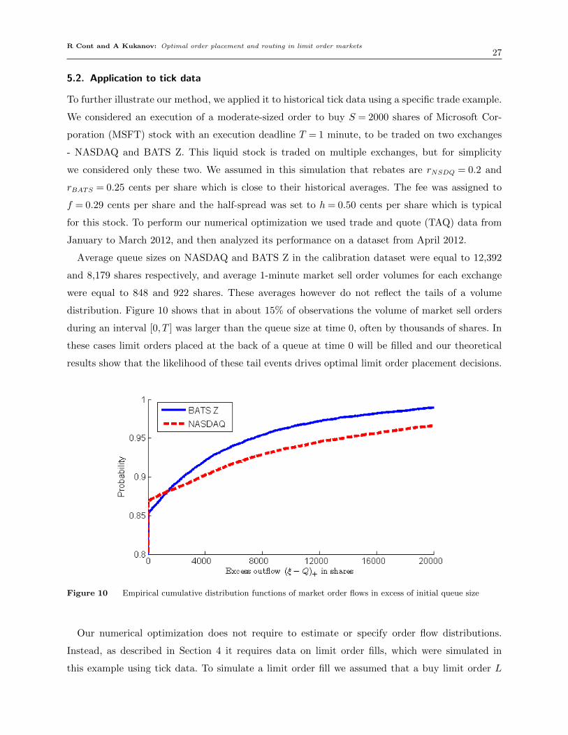
distribution. Figure 10 shows that in about 15% of observations the volume of market sell orders
during an interval [0, T ] was larger than the queue size at time 0, often by thousands of shares. In
these cases limit orders placed at the back of a queue at time 0 will be filled and our theoretical
results show that the likelihood of these tail events drives optimal limit order placement decisions.
Figure 10 Empirical cumulative distribution functions of market order flows in excess of initial queue size
Our numerical optimization does not require to estimate or specify order flow distributions.
Instead, as described in Section 4 it requires data on limit order fills, which were simulated in
this example using tick data. To simulate a limit order fill we assumed that a buy limit order L
R Cont and A Kukanov: Optimal order placement and routing in limit order markets28
placed behind a queue of Q shares at the best bid is filled if the volume of sell market orders
during its placement horizon (T = 1 minute in our example) is larger than Q. The execution is
complete if the volume of sell market orders exceeds Q by more than L, otherwise it is a partial
execution. One-minute sell market order volumes were estimated as a sum of trade sizes at a given
exchange whose trade prices were equal to the prevailing bid price. In this simulation we made
several simplifications that are related to TAQ data limitations. First, our limit order fill estimates
are conservative as they do not include possible order cancelations from the front of a bid queue.
TAQ data does not have information on order cancelations, but this information is available in
more detailed “level-2” datasets. Second, buy limit orders can be filled when ask price ticks down,
but estimating these fills accurately requires knowledge of order queue position which is unavailable
in TAQ. To simplify our simulation we restricted it to one-minute samples where the best quotes
did not change up or down.
To estimate sensitivity to queue sizes QBATS or QNSDQ we ranked observations by queue sizes
QBATS,QNSDQ and grouped them into three equal sized bins labeled “high”, “medium” and “low”.
Similarly we ranked, grouped and labeled observations by total trading volume in the previous
minute V OLBATS, V OLNSDQ. Each label was then used as a state variable leading to 34 = 81 dif-
ferent combinations of state variables. Each combination of states defined a subsample of historical
data, which we used to simulate limit order fills. Based on simulated limit order fills we computed
a numerical solution for each subsample following the algorithm from Section 4.
The result is a lookup table where one can find an approximate solution for each of 81
state variable combinations. Order allocations in this table take into account the magnitude of
QBATS,QNSDQ and V OLBATS, V OLNSDQ relative to their historical values. We recomputed order
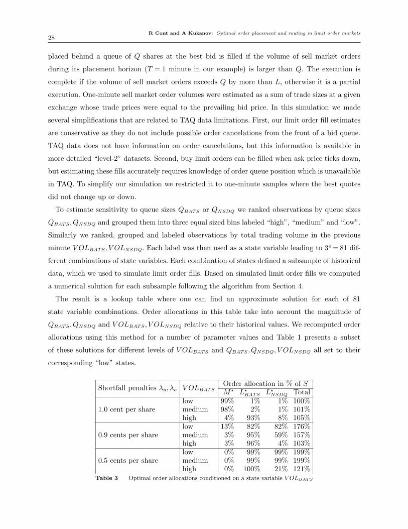
allocations using this method for a number of parameter values and Table 1 presents a subset
of these solutions for different levels of V OLBATS and QBATS,QNSDQ, V OLNSDQ all set to their
corresponding “low” states.
Shortfall penalties λu, λo V OLBATSOrder allocation in % of SM? L?BATS L?NSDQ Total
1.0 cent per sharelow 99% 1% 1% 100%medium 98% 2% 1% 101%high 4% 93% 8% 105%
0.9 cents per sharelow 13% 82% 82% 176%medium 3% 95% 59% 157%high 3% 96% 4% 103%
0.5 cents per sharelow 0% 99% 99% 199%medium 0% 99% 99% 199%high 0% 100% 21% 121%
Table 3 Optimal order allocations conditioned on a state variable V OLBATS
R Cont and A Kukanov: Optimal order placement and routing in limit order markets29
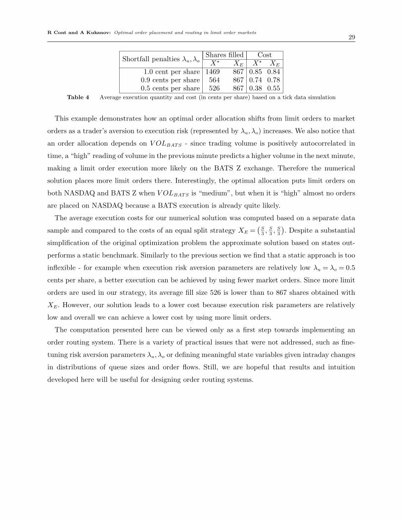
Shortfall penalties λu, λoShares filled CostX? XE X? XE
1.0 cent per share 1469 867 0.85 0.840.9 cents per share 564 867 0.74 0.780.5 cents per share 526 867 0.38 0.55
Table 4 Average execution quantity and cost (in cents per share) based on a tick data simulation
This example demonstrates how an optimal order allocation shifts from limit orders to market
orders as a trader’s aversion to execution risk (represented by λu, λo) increases. We also notice that
an order allocation depends on V OLBATS - since trading volume is positively autocorrelated in
time, a “high” reading of volume in the previous minute predicts a higher volume in the next minute,
making a limit order execution more likely on the BATS Z exchange. Therefore the numerical
solution places more limit orders there. Interestingly, the optimal allocation puts limit orders on
both NASDAQ and BATS Z when V OLBATS is “medium”, but when it is “high” almost no orders
are placed on NASDAQ because a BATS execution is already quite likely.
The average execution costs for our numerical solution was computed based on a separate data
sample and compared to the costs of an equal split strategy XE =(S3, S3, S3
). Despite a substantial
simplification of the original optimization problem the approximate solution based on states out-
performs a static benchmark. Similarly to the previous section we find that a static approach is too
inflexible - for example when execution risk aversion parameters are relatively low λu = λo = 0.5
cents per share, a better execution can be achieved by using fewer market orders. Since more limit
orders are used in our strategy, its average fill size 526 is lower than to 867 shares obtained with
XE. However, our solution leads to a lower cost because execution risk parameters are relatively
low and overall we can achieve a lower cost by using more limit orders.
The computation presented here can be viewed only as a first step towards implementing an
order routing system. There is a variety of practical issues that were not addressed, such as fine-
tuning risk aversion parameters λu, λo or defining meaningful state variables given intraday changes
in distributions of queue sizes and order flows. Still, we are hopeful that results and intuition
developed here will be useful for designing order routing systems.
R Cont and A Kukanov: Optimal order placement and routing in limit order markets30
6. Conclusion
We have formulated the optimal order placement problem for a market participant able to submit
market orders and limit orders across multiple exchanges, and studied its solution properties using
historical data and numerical simulations. In the case when only one exchange is available we
have derived an optimal split between limit and market orders and showed that an optimal order
allocation depends on trader’s aversion to execution risk. For the general case of multiple exchanges,
we provide a characterization of the optimal order placement strategy in terms of execution shortfall
probabilities. To solve the problem in practical applications we propose a fast and straightforward
numerical algorithm that re-samples past order fill data to optimize future order executions. Using
this algorithm, we have studied the sensitivities of an optimal order allocation to problem inputs
and showed that a simultaneous placement of limit orders on multiple trading venues according to
our method can lead to a substantial reduction of transaction costs.
Appendix. A: Alternative problem formulation
We may also consider an alternative approach to order placement optimization, which turns out
to be related to our original formulation by duality. Consider the following problem:
Problem 2 (Alternative formulation: cost minimization under execution constraints)
minX∈RK+1
+
E
[(h+ f)M −
K∑k=1
(h+ rk)((ξk−Qk)+− (ξk−Qk−Lk)+)
+θ
(M +
K∑k=1
Lk + (S−A(X,ξ))+
)](13)
subject to: E[(S−A(X,ξ))+
]≤ µu (14)
E[(A(X,ξ)−S)+
]≤ µo (15)
In this alternative formulation a trader can specify his tolerance to execution risks using constraints
on expected order shortfalls and overflows. The goal is to minimize an expectation of order execution
costs under expected shortfall constraints. The Problem 2 does not appear to be tractable, but it
has a convex objective and convex inequality constraints, and we can easily find its (Lagrangian)
dual problem:
Problem 3
maxλu≥0,λo≥0
{V ?(λu, λo)−λuµu−λoµo} (16)
where V ?(λu, λo) = minX∈RK+1
+
E[v(X,ξ)] is the optimal objective value from Problem 1 given parameter
values λu, λo.
R Cont and A Kukanov: Optimal order placement and routing in limit order markets31
We see that the Problem 3 is related to our original order placement problem - solving the Problem
3 (and therefore, the Problem 2) amounts to re-solving the Problem 1 for different values of λu, λo.
This discussion also leads to a new interpretation of parameters λu, λo in the Problem 1 as shadow
prices for expected shortfall and overflow constraints in the related Problem 2. Hereafter we focus
on the (more tractable) Problem 1, but note that the optimal point for the Problem 2 can also be
found by solving its dual problem.
Appendix. B: Proofs
Proof of Proposition 1 First, for any allocation X that has M > S, we automatically have
A(X) > S and we can show that the (random) costs of X are larger than those of XM =
(S,0, . . . ,0)∈ C:
v(X, ξ)− v(XM , ξ) = (h+ f)(M −S)−K∑k=1
(h+ rk)((ξk−Qk)+− (ξk−Qk− Lk)+)+
λo
(M −S+
K∑k=1
((ξk−Qk)+− (ξk−Qk− Lk)+
))+ θ(M −S+
K∑k=1
Lk)>
(λo +h+ f)(M −S) +K∑k=1
(λo−h− rk)((ξk−Qk)+− (ξk−Qk−Lk)+)> 0,
which holds for all random ξ. Therefore, V (X) > V (XM). Similarly, for any allocation X with
Lk >S− M define a new allocation X ′ by setting M ′ = M , L′j = Lj,∀j 6= k and L′k = S− M . Then
v(X, ξ)− v(X ′, ξ) = θ(Lk− L′k)> 0 on the event B = {ω|ξk(ω)<Qk +S−M}.
On a complementary event Bc,
v(X, ξ)− v(X ′, ξ) =−(h+ rk)((ξk−Qk−S+ M)+− (ξk−Qk− Lk)+)
+λo((ξk−Qk−S+ M)+− (ξk−Qk− Lk)+) + θ(Lk− L′k).
Therefore
V (X)−V (X ′) =E[v(X, ξ)− v(X ′, ξ)|B
]P(B) +E
[v(X, ξ)− v(X ′, ξ)|Bc
]P(Bc) =
θ(Lk− L′k) +E[(λo− (h+ rk))((ξk−Qk−S+ M)+− (ξk−Qk− Lk)+)|Bc
]P(Bc)> 0
If X ′ /∈ C, we can continue truncating limit order sizes L′j >S − M ′ to S − M ′ following the same
argument. Each time the truncation decreases the objective function and finally we obtain a X ′′ ∈ C,
such that V (X ′′)<V (X).
R Cont and A Kukanov: Optimal order placement and routing in limit order markets32
Next, if X is such that M−∑K
k=1 Lk <S consider the difference s= S−M−∑K
k=1 Lk and define a
new allocation X ′ as M ′ = M+s, L′k = Lk, k= 1, . . . ,K. Then v(X ′, ξ)−v(X, ξ) = (h+f−λu)s < 0.
Although the total quantity of orders in allocation X is smaller than in X ′, it has the same market
impact. The former always falls short of the target S and its remainder s must be filled with a
market order at time T , leading to the same impact. Since v(X ′, ξ)− v(X, ξ) < 0, we also have
V (X ′)<V (X). �
Proof of Proposition 2: First, note that (ξk−Qk)+−(ξk−Qk−Lk)+ are concave functions of Lk.
Therefore, A(X,ξ) is concave as a sum of concave functions. Similarly, the cost term in v(X,ξ) is
a sum of convex functions, as long as rk ≥−h,k= 1, . . . ,K and is itself a convex function. Second,
since S −A(X,ξ) is a convex functon of X, and the function h(x) = λu(x)+ − λo(−x)+ is convex
in x for positive λu, λo, so the penalty term h (S−A(X,ξ))) is also convex.
Using the assumption λo > h+ maxk{rk} it is clear that the function v(X,ξ) is bounded from
below by −(h+ maxk{rk})S and therefore V (X) is also bounded from below.
Since V (X) is convex, it is also continous and since it is bounded from below it reaches a
local minimum Vmin on the compact set C at some point X? ∈ C. By convexity, Vmin is a global
minimum of V (X) on C. Moreover, Proposition 1 guarantees that Vmin <V (X) for any X /∈ C, so
Vmin is also a global minimum of V (X) on RK+1+ . �
Proof of Proposition 3:
By Proposition 1 there exists an optimal split (M?,L?) ∈ C between limit and market orders.
Moreover for K = 1 the set C reduces to a line M? + L? = S so it is sufficient to find M?. The
restriction L= S −M implies that {A(X,ξ)> S}= ∅, {A(X,ξ)< S,ξ >Q+L}= ∅, and we can
rewrite the objective function as
V (M) =E[(h+ f)M − (h+ r)((ξ−Q)+− (ξ−Q−S+M)+) + θS +
(λu + θ) (S−M − ((ξ−Q)+− (ξ−Q−S+M)+))))+
]. (17)
Although θS is a constant, we note that different solutions (M,L) have different total market impact
due to a terminal market order at time T . For M ∈ (0, S) the expression under the expectation in
(17) is bounded for all ξ and Lipschitz with respect to M , so we can compute V ′(M) = dV (M)
dMas:
V ′(M) =E[h+ f + (h+ r)1{ξ>Q+S−M}− (λu + θ)1{ξ<Q+S−M}
]= 2h+ f + r− (h+ r+λu + θ)F (Q+S−M) (18)
R Cont and A Kukanov: Optimal order placement and routing in limit order markets33
Note that if λu ≤2h+ f + r
F (Q+S)− (h + r + θ), then V ′(M) ≥ 0 for M ∈ (0, S) and therefore V is
non-decreasing at these points. Checking that
V (S)−V (0)≥ (h+ f −λu− θ)S+ (λu + θ+h+ r)S(1−F (Q+S))≥ 0
we conclude that M? = 0. Similarly, if λu ≥2h+ f + r
F (Q)− (h+ r+ θ), then V ′(M)≤ 0 for all M ∈
(0, S) and V (M) is non-increasing at these points. Checking that
V (S)−V (0)≤ (h+ f −λu− θ)S+ (λu + θ+h+ r)S(1−F (Q))≤ 0
we conclude that M? = S. Finally, if λu is between these two values, ∃ε > 0, such that
V ′(ε) < 0, V ′(S − ε) > 0 and by continuity of V ′ there is a point where V ′(M?) = 0. This M? is
optimal by convexity of V (M) and (9) solves equations V ′(M?) = 0,L? = S−M?. �
Proof of Proposition 4:
Proposition 2 implies the existence of an optimal order allocation X? ∈ C. First, we define XM =
(S,0, . . . ,0) and prove that X? 6=XM by contradiction. If XM were optimal in the problem (6) it
would also be optimal in the same problem with a constraint Lk = 0, k 6= j, for any one j. In other
words, the solution (S,0) would be optimal for any one-exchange problem, defined by using only
exchange j. But by our assumption, there exists a J such that λu <2h+ f + rJFJ(QJ)
− (h+ rJ) and
Proposition 3 implies that (S,0) is not optimal for the J-th single-exchange subproblem, leading
to a contradiction.
The function v(X,ξ) is bounded for X ∈ C and for all ξ, differentiable with respect to M and
Lk, k= 1, . . . ,K for X ∈ C\{XM} for almost all ξ. Therefore V (X) is differentiable for X ∈ C\{XM}
and we can compute all of its partial derivatives by interchanging the order of differentiation and
integration. The KKT conditions for problem (6) and X ∈ C\{XM} are
h+ f + θ− (λu + θ)P(A(X?, ξ)<S) +λoP(A(X?, ξ)>S)−µ0 = 0 (19)
− (h+ rk)P(ξk >Qk +L?k) + θ− (λu + θ)P(A(X?, ξ)<S,ξk >Qk +L?k)+
λoP(A(X?, ξ)>S,ξk >Qk +L?k)−µk = 0, k= 1, . . . ,K (20)
M ≥ 0, Lk ≥ 0, µ0 ≥ 0, µk ≥ 0, µ0M = 0, µkLk = 0, k= 1, . . . ,K (21)
Since the objective function V (·) is convex, conditions (19)–(21) are both necessary and sufficient
for optimality. The first result of this proposition follows if we consider any X with M = 0 and use
the assumption λu ≥2h+f+max
k{rk}
p0− (h+ max
k{rk}):
R Cont and A Kukanov: Optimal order placement and routing in limit order markets34
V (X)≥−(h+maxk{rk})SP
(⋂k
{ξk ≤Qk}
)+λuSP
(⋂k
{ξk ≤Qk}
)+θS ≥ (h+f+θ)S = V (XM).
We already argued that ∃X? with V (X?)<V (XM), so X? 6= X and therefore M? > 0.
Next, we can rearrange terms in a j-th equality (20) as follows:
θ+P(ξj >Qj +L?j )[λo− (h+ rj)− (λu +λo + θ)P(A(X?, ξ)<S|ξj >Qj +L?j )
]−µj = 0. (22)
Setting L?j = 0 and using the assumption (h+ rj − λo)P (ξj >Qj) > θ we see that equation (22)
cannot hold because the left-hand side is negative, leading to a contradiction.
We showed that M? > 0,L?j > 0 for all j = 1, . . . ,K and therefore, µ0 = µ1 = · · · = µK = 0 by
complementary slackness. Then the KKT conditions (19)–(21) reduce to (10)–(11). �
Corollary In addition to assumptions of Proposition 4, assume that K = 2 and ξ1, ξ2 are
independent. Also, assume that F1,2(Q1,2)< 1− h+ r2,1λo
and (h+ r1,2)P (ξ1,2 >Q1,2 +S)> θ. Then
there is an optimal order allocation X? = (M?,L?1,L?2)∈ int{C} and it solves equations (12a-12c).
Proof: First we show that solutions on the boundary of C are sub-optimal: M? = 0, M? = S and
L?1,2 = 0 are ruled out in Proposition 4. Solutions with M? +K∑k=1
L?k = S are ruled out by checking
(20) and noting that since A(X?, ξ) > S = ∅ and (h+ rj)P (ξj >Qj +S) > θ by assumption, the
left-hand side of that equation is always negative, leading to a contradiction.
Finally, solutions with L1,2 = S −M are also ruled out by checking (20). For example, if L1 =
S−M > 0 it follows that µ1 = 0 and we can rewrite (20) as:
−(h+ r1)P(ξ1 >Q1 +L1) + θ+λoP(ξ2 >Q2)P(ξ1 >Q1 +L1) = 0
Dividing by P(ξ1 >Q1 +L1) and applying the assumption F1(Q1)< 1− h+ r2λo
we note that the
left-hand side of the equation is always positive leading to a contradiction.
Having showed that an optimal solution belongs to the interior of C, we can simplify the descrip-
tion of an event A(X,ξ)>S. For any X ∈ int{C}, A(X,ξ)>S if and only if all the following three
inequalities are satisfied:
ξ1 >Q1 +S−M −L2 (23a)
ξ2 >Q2 +S−M −L1 (23b)
ξ1 + ξ2 >Q1 +Q2 +S−M (23c)
R Cont and A Kukanov: Optimal order placement and routing in limit order markets35
These inequalities give a simple characterization of the event {A(X,ξ) > S} which is directly
verified by considering subsets of (ξ1, ξ2) forming a complete partition of R2+.
Case 1: ξ1 >Q1 +L1, ξ2 >Q2 +L2. Since L1 +L2 +M >S, we have A(X,ξ) =L1 +L2 +M >S
and at the same time all of the inequalities (23a-23c) are satisfied, so they are trivially equivalent
in this case.
Case 2: ξ1 >Q1 +L1,Q2 ≤ ξ2 ≤Q2 +L2. Because of the condition ξ1 >Q1 +L1, (23a) is satisfied.
We have in this case that A(X,ξ) =L1 + ξ2−Q2 +M and thus A(X,ξ)>S if and only if (23b) is
satisfied. Finally, ξ1 >Q1 +L1 together with (23b) imply (23c), so A(X,ξ)> S and (23a-23c) are
equivalent in this case.
Case 3: ξ2 > Q2 + L2,Q1 ≤ ξ1 ≤ Q1 + L1. Similarly to Case 2 we can show that inequalities
(23a-23c) are satisfied if and only if A(X,ξ)>S.
Case 4: Q1 + S −M − L2 < ξ1 ≤ Q1 + L1,Q2 + S −M − L1 < ξ2 ≤ Q2 + L2. This set is non-
empty because 0<S−M −L1 <L2 and similarly for L1,L2 reversed. Inequalities (23a)–(23b) hold
trivially, only (23c) needs to be checked. We can write A(X,ξ) = ξ1−Q1 + ξ2−Q2 +M >S if and
only if (23c) holds, so A(X,ξ)>S is equivalent to (23a-23c).
Case 5: Outside of Cases 1-4, either (23a) or (23b) is not satisfied. If ξ1 ≤Q1 +S−M −L2, ξ2 ≤Q2 +L2, then A(X,ξ)≤ S−M −L2 +L2 +M = S. The case ξ2 ≤Q2 +S−M −L1, ξ1 ≤Q1 +L1 is
completely symmetric, and it shows that neither A(X,ξ)>S nor (23a-23c) hold in this case.
Next, we use inequalities (23a-23c) to characterize the set {A(X,ξ)>S} in the first-order conditions
(10)–(11). We observe that in the two-exchange case
{A(X,ξ)>S,ξ1 >Q1 +L1}= {ξ1 >Q1 +L1, ξ2 >Q2 +S−M −L1}
{A(X,ξ)>S,ξ2 >Q2 +L2}= {ξ2 >Q2 +L2, ξ1 >Q1 +S−M −L2},
and then use the independence of ξ1 and ξ2 to compute
P(A(X,ξ)>S|ξ1 >Q1 +L1) = F2(Q2 +S−M −L1)
P(A(X,ξ)>S|ξ2 >Q2 +L2) = F1(Q1 +S−M −L2)
Together with (11), this leads to a pair of equations for limit orders sizes:
F2(Q2 +S−M −L1) =−θ/F1(Q1 +L1) +λu + θ+h+ r1
λu +λo + θ
F1(Q1 +S−M −L2) =−θ/F2(Q2 +L2) +λu + θ+h+ r2
λu +λo + θ
whose solution is given by L?1,L?2 from (12a,12b). To obtain the equation (12c), we rewrite the first
equation in (10,11) using the inequalities (23a-23c). Then P (A(X,ξ)>S) may be computed as the
integral of the product measure F1⊗F2 over the region defined by
U(Q,S,M,L1,L2) = {(x1, x2)∈R2, x1 >Q1+S−M−L2, x2 >Q2+S−M−L1, x1+x2 >Q1+Q2+S−M}.
R Cont and A Kukanov: Optimal order placement and routing in limit order markets36
This integral is given by
P (A(X,ξ)>S) = F1⊗F2 (U(Q,S,M,L1,L2))
= F1(Q1 +L1)F2(Q2 +S−M −L1) +
Q1+L1∫Q1+S−M−L2
F2(Q1 +Q2 +S−M −x1)dF1(x1) =λu− (h+ f)
λu +λo + θ
�
R Cont and A Kukanov: Optimal order placement and routing in limit order markets37
References
Alfonsi, Aurelien, Antje Fruth, Alexander Schied. 2010. Optimal execution strategies in limit order books
with general shape functions. Quantitative Finance 10(2) 143–157.
Almgren, R, N Chriss. 2000. Optimal execution of portfolio transactions. Journal of Risk 3 5–39.
Almgren, R, W. Harts. 2008. A Dynamic Algorithm for Smart Order Routing. Tech. rep., StreamBase.
Almgren, R, C Thum, E Hauptmann, H Li. 2005. Direct Estimation of Equity Market Impact. Risk 18 57.
Baron, Matthew, Jonathan Brogaard, Andrei Kirilenko. 2014. Risk and returns in high frequency trading.
Tech. rep.
Battalio, Robert, Shane Corwin, Robert Jennings. 2013. Can Brokers Have it all? On the Relation between
Make Take Fees & Limit Order Execution Quality. Working paper.
Bayraktar, Erhan, Michael Ludkovski. 2011. Optimal Trade Execution in Illiquid Markets. Mathematical
Finance 21(4) 681–701.
Bertsimas, D, Andrew W Lo. 1998. Optimal control of execution costs. Journal of Financial Markets 1(1)
1–50.
Boehmer, Ekkehart, Robert Jennings. 2007. Public disclosure and private decisions: Equity market execution
quality and order routing. Review of Financial Studies 20(2) 315–358.
Brogaard, Jonathan, Corey Garriott, Anna Pomeranets. 2014. High-Frequency Trading Competition.
Cao, Charles, Oliver Hansch, Xiaoxin Wang. 2008. Order placement strategies in a pure limit order book
market. Journal of Financial Research 31(2) 113–140.
Cont, Rama. 2011. Statistical modeling of high-frequency financial data. IEEE Signal Processing 28(5)
16–25.
Cont, Rama, Adrien De Larrard. 2013. Price dynamics in a Markovian limit order market. SIAM Journal
on Financial Mathematics 4(1) 1–25.
Cont, Rama, Arseniy Kukanov, Sasha Stoikov. 2014. Price impact of order book events. Journal of Financial
Econometrics 12(1) 47–88.
Eisler, Zoltan, Jean-Philippe Bouchaud, Julien Kockelkoren. 2012. The price impact of order book events:
market orders, limit orders and cancellations. Quantitative Finance 12(9) 1395–1419.
Foucault, T, A.J. Menkveld. 2008. Competition for Order Flow and Smart Order Routing Systems. Journal
of Finance 63(1) 112.
Foucault, Thierry. 1999. Order flow composition and trading costs in a dynamic limit order market. Journal
of Financial Markets 2(2) 99–134.
Foucault, Thierry, O Kadan, Eugene Kandel. 2005. Limit Order Book as a Market for Liquidity. Review of
Financial Studies 18(4) 1171–1217.
R Cont and A Kukanov: Optimal order placement and routing in limit order markets38
Ganchev, Kuzman, Yuriy Nevmyvaka, Michael Kearns. 2010. Censored exploration and the dark pool prob-
lem. Communications of the ACM 53(5) 99.
Glosten, L, P Milgrom. 1985. Bid, ask and transaction prices in a specialist market with heterogeneously
informed traders. Journal of Financial Economics 14 71–100.
Gueant, Olivier, C.A. Lehalle. 2014. General Intensity Shapes in Optimal Liquidation. Mathematical Finance
to appear.
Guilbaud, Fabien, Huyen Pham. 2014. Optimal high frequency trading in a pro-rata microstructure with
predictive information. Mathematical Finance to appear.
Guo, Xin, Adrien De Larrard, Z Ruan. 2013. Optimal Placement in a Limit Order Book.
Harris, Lawrence, Joel Hasbrouck. 1996. Market vs. limit orders: the SuperDOT evidence on order submission
strategy. Journal of Financial and Quantitative Analysis 31(2) 213–231.
Huberman, Gur, Werner Stanzl. 2005. Optimal liquidity trading. Review of Finance 9(2) 165–200.
Huitema, Robert. 2012. Optimal Portfolio Execution using Market and Limit Orders.
Kushner, Harold, George Yin. 2003. Stochastic Approximation and Recursive Algorithms and Applications.
Springer, New York.
Kyle, A.S. 1985. Continuous auctions and insider trading. Econometrica 1315–1335.
Laruelle, Sophie, Charles-Albert Lehalle, Gilles Pages. 2011. Optimal split of orders across liquidity pools:
a stochastic algorithm approach. SIAM Journal on Financial Mathematics 2(1) 1042–1076.
Li, Tianhui Michael. 2013. Optimal Limit-versus-Market Order Slicing under a VWAP Bechmark - Contin-
uous Case.
Lynch, Sarah, Emily Flitter. 2014. SEC probing brokerages over handling of retail orders. Reuters .
Mastromatteo, I, B. Toth, Jean-Philippe Bouchaud. 2013. Agent-based models for latent liquidity and
concave price impact.
Menkveld, A.J. 2013. High frequency trading and the new-market makers. Journal of Financial Markets
16(4) 712–740.
Moallemi, C.C., Constantinos Maglaras, Hua Zheng. 2012. Optimal Order Routing in a Fragmented Market.
Working Paper DRO-2012-02, Columbia University.
Nemirovski, A, A Juditsky, G Lan, A Shapiro. 2009. Robust stochastic approximation approach to stochastic
programming. SIAM Journal on Optimization 19(4) 1574–1609.
Obizhaeva, Anna A, Jiang Wang. 2012. Optimal trading strategy and supply/demand dynamics. Journal of
Financial Markets 16(1) 1–32.
Parlour, Christine. 1998. Price dynamics in limit order markets. Review of Financial Studies 11(4) 789–816.
R Cont and A Kukanov: Optimal order placement and routing in limit order markets39
Phillips, Matthew. 2014. What’s E*Trade Doing With Its Customers’ Orders Anyway? Bloomberg Business-
week .
Predoiu, Silviu, Gennady Shaikhet, Steven Shreve. 2011. Optimal Execution in a General One-Sided Limit-
Order Book. SIAM Journal on Financial Mathematics 2(1) 183–212.
Rosu, Ioanid. 2009. A Dynamic Model of the Limit Order Book. Review of Financial Studies 22(11) 4601.
U.S. Senate. 2014. Conflicts of Interest in the U.S. Equity Markets: Testimony of Robert Battalio. Permanent
Subcommittee on Investigations of the Committee on Homeland Security and Governmental Affairs .
Williamson, David P, David B Shmoys. 2011. The design of approximation algorithms. Cambridge University
Press.