The Impact of a Barrier Island Loss on Extreme Events in...
15
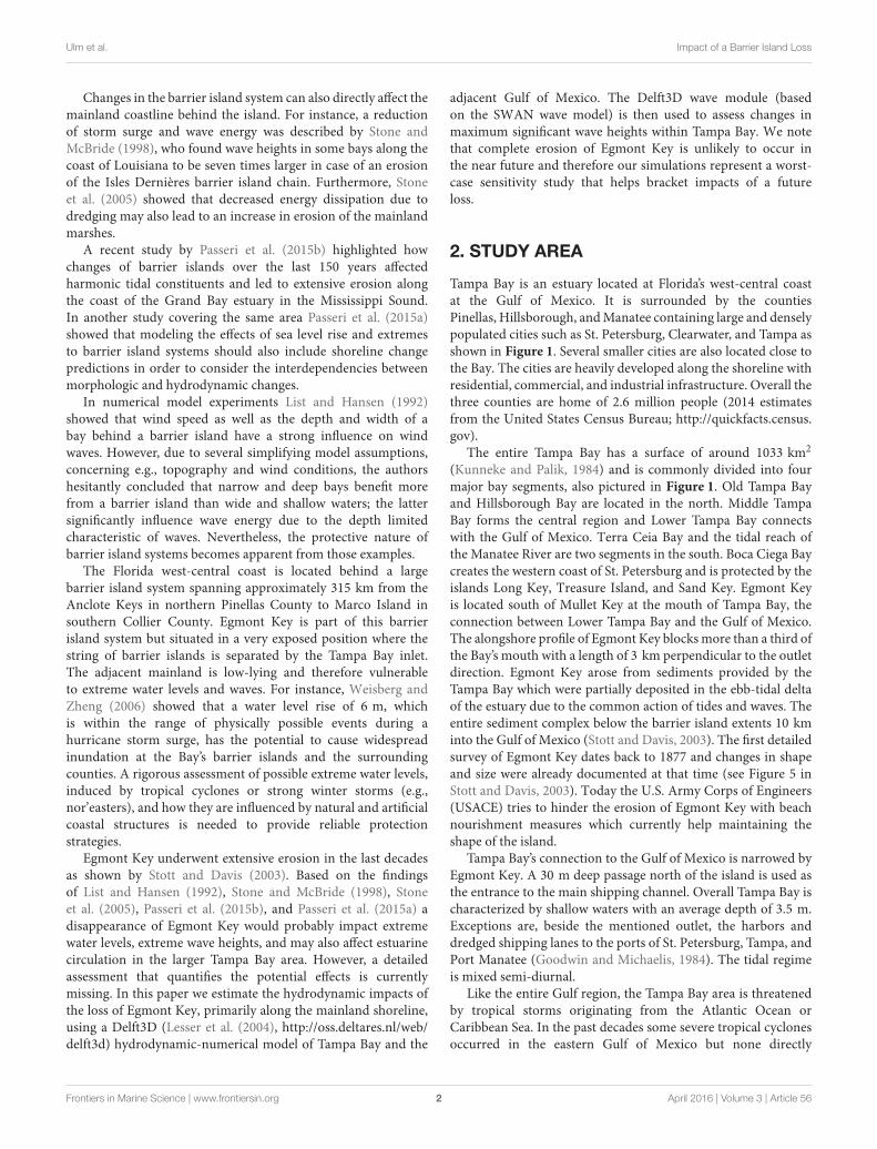
ORIGINAL RESEARCH published: 29 April 2016 doi: 10.3389/fmars.2016.00056 Frontiers in Marine Science | www.frontiersin.org 1 April 2016 | Volume 3 | Article 56 Edited by: Ivan David Haigh, University of Southampton, UK Reviewed by: Matthew John Eliot, Damara WA Pty Ltd., Australia Pushpa Dissanayake, University of Konstanz, Germany *Correspondence: Marius Ulm [email protected] Specialty section: This article was submitted to Coastal Ocean Processes, a section of the journal Frontiers in Marine Science Received: 16 December 2015 Accepted: 11 April 2016 Published: 29 April 2016 Citation: Ulm M, Arns A, Wahl T, Meyers SD, Luther ME and Jensen J (2016) The Impact of a Barrier Island Loss on Extreme Events in the Tampa Bay. Front. Mar. Sci. 3:56. doi: 10.3389/fmars.2016.00056 The Impact of a Barrier Island Loss on Extreme Events in the Tampa Bay Marius Ulm 1 *, Arne Arns 1 , Thomas Wahl 1, 2 , Steven D. Meyers 2 , Mark E. Luther 2 and Jürgen Jensen 1 1 Department of Civil Engineering, Research Institute for Water and Environment, University of Siegen, Siegen, Germany, 2 Ocean Monitoring and Prediction Laboratory, College of Marine Science, University of South Florida, St. Petersburg, FL, USA Barrier islands characterize up to an eighth of the global coastlines. They buffer the mainland coastal areas from storm surge and wave energy from the open ocean. Changes in their shape or disappearance due to erosion may lead to an increased impact of sea level extremes on the mainland. A barrier island threatened by erosion is Egmont Key which is located in the mouth of the Tampa Bay estuary at the west-central coast of Florida. In this sensitivity study we investigate the impact a loss of Egmont Key would have on storm surge water levels and wind waves along the coastline of Tampa Bay. We first simulate still water levels in a control run over the years 1948–2010 using present-day bathymetry and then in a scenario run covering the same period with identical boundary conditions but with Egmont Key removed from the bathymetry. Return water levels are assessed for the control and the scenario runs using the Peak-over-threshold method along the entire Tampa Bay coastline. Egmont Key is found to have a significant influence on the return water levels in the Bay, especially in the northern, furthest inland parts where water levels associated with the 100-year return period increase between 5 and 15cm. Additionally, wind wave simulations considering all 99.5th percentile threshold exceedances in the years 1980–2013 were conducted with the same control and scenario bathymetries. Assessing changes in return levels of significant wave heights due to the loss of Egmont Key revealed an increase of significant wave heights around today’s location of the island. Keywords: barrier islands, beach erosion, numerical modeling, extreme value statistics, extreme water levels, extreme wave heights, estuary, Tampa Bay 1. INTRODUCTION Barrier islands are located near the mainland coast, often forming lagoons which are connected to the ocean by small tidal inlets. Oertel (1985) describes that coastal areas around and behind a barrier island are not merely independent from each other but rather part of an interrelated barrier island system with regard to hydrodynamic, hydrological, and geological processes. Globally, barrier islands can be found along 6.5% (Stutz and Pilkey, 2001) to 13% (Cromwell, 1973) of the coastlines. Examples in Europe are the Frisian Islands protecting the Wadden Sea (North Sea) or the barrier island system forming the Venice Lagoon (Mediterranean Sea). In the United States barrier island systems span large coastal areas along the Atlantic Ocean and Gulf of Mexico. Due to marked interdependency between barrier islands, the mainland coast, and adjacent waters, changes in individual parts may have an effect on the entire system (Oertel, 1985).
Transcript of The Impact of a Barrier Island Loss on Extreme Events in...

ORIGINAL RESEARCHpublished: 29 April 2016
doi: 10.3389/fmars.2016.00056
Frontiers in Marine Science | www.frontiersin.org 1 April 2016 | Volume 3 | Article 56
Edited by:
Ivan David Haigh,
University of Southampton, UK
Reviewed by:
Matthew John Eliot,
Damara WA Pty Ltd., Australia
Pushpa Dissanayake,
University of Konstanz, Germany
*Correspondence:
Marius Ulm
Specialty section:
This article was submitted to
Coastal Ocean Processes,
a section of the journal
Frontiers in Marine Science
Received: 16 December 2015
Accepted: 11 April 2016
Published: 29 April 2016
Citation:
Ulm M, Arns A, Wahl T, Meyers SD,
Luther ME and Jensen J (2016) The
Impact of a Barrier Island Loss on
Extreme Events in the Tampa Bay.
Front. Mar. Sci. 3:56.
doi: 10.3389/fmars.2016.00056
The Impact of a Barrier Island Losson Extreme Events in the Tampa BayMarius Ulm 1*, Arne Arns 1, Thomas Wahl 1, 2, Steven D. Meyers 2, Mark E. Luther 2 and
Jürgen Jensen 1
1Department of Civil Engineering, Research Institute for Water and Environment, University of Siegen, Siegen, Germany,2Ocean Monitoring and Prediction Laboratory, College of Marine Science, University of South Florida, St. Petersburg, FL,
USA
Barrier islands characterize up to an eighth of the global coastlines. They buffer the
mainland coastal areas from storm surge and wave energy from the open ocean.
Changes in their shape or disappearance due to erosion may lead to an increased impact
of sea level extremes on the mainland. A barrier island threatened by erosion is Egmont
Key which is located in the mouth of the Tampa Bay estuary at the west-central coast
of Florida. In this sensitivity study we investigate the impact a loss of Egmont Key would
have on storm surge water levels and wind waves along the coastline of Tampa Bay. We
first simulate still water levels in a control run over the years 1948–2010 using present-day
bathymetry and then in a scenario run covering the same period with identical boundary
conditions but with Egmont Key removed from the bathymetry. Return water levels are
assessed for the control and the scenario runs using the Peak-over-threshold method
along the entire Tampa Bay coastline. Egmont Key is found to have a significant influence
on the return water levels in the Bay, especially in the northern, furthest inland parts
where water levels associated with the 100-year return period increase between 5 and
15 cm. Additionally, wind wave simulations considering all 99.5th percentile threshold
exceedances in the years 1980–2013 were conducted with the same control and
scenario bathymetries. Assessing changes in return levels of significant wave heights
due to the loss of Egmont Key revealed an increase of significant wave heights around
today’s location of the island.
Keywords: barrier islands, beach erosion, numerical modeling, extreme value statistics, extreme water levels,
extreme wave heights, estuary, Tampa Bay
1. INTRODUCTION
Barrier islands are located near the mainland coast, often forming lagoons which are connected tothe ocean by small tidal inlets. Oertel (1985) describes that coastal areas around and behind a barrierisland are not merely independent from each other but rather part of an interrelated barrier islandsystem with regard to hydrodynamic, hydrological, and geological processes. Globally, barrierislands can be found along 6.5% (Stutz and Pilkey, 2001) to 13% (Cromwell, 1973) of the coastlines.Examples in Europe are the Frisian Islands protecting the Wadden Sea (North Sea) or the barrierisland system forming the Venice Lagoon (Mediterranean Sea). In the United States barrier islandsystems span large coastal areas along the Atlantic Ocean and Gulf of Mexico. Due to markedinterdependency between barrier islands, the mainland coast, and adjacent waters, changes inindividual parts may have an effect on the entire system (Oertel, 1985).
Ulm et al. Impact of a Barrier Island Loss
Changes in the barrier island system can also directly affect themainland coastline behind the island. For instance, a reductionof storm surge and wave energy was described by Stone andMcBride (1998), who found wave heights in some bays along thecoast of Louisiana to be seven times larger in case of an erosionof the Isles Dernières barrier island chain. Furthermore, Stoneet al. (2005) showed that decreased energy dissipation due todredging may also lead to an increase in erosion of the mainlandmarshes.
A recent study by Passeri et al. (2015b) highlighted howchanges of barrier islands over the last 150 years affectedharmonic tidal constituents and led to extensive erosion alongthe coast of the Grand Bay estuary in the Mississippi Sound.In another study covering the same area Passeri et al. (2015a)showed that modeling the effects of sea level rise and extremesto barrier island systems should also include shoreline changepredictions in order to consider the interdependencies betweenmorphologic and hydrodynamic changes.
In numerical model experiments List and Hansen (1992)showed that wind speed as well as the depth and width of abay behind a barrier island have a strong influence on windwaves. However, due to several simplifying model assumptions,concerning e.g., topography and wind conditions, the authorshesitantly concluded that narrow and deep bays benefit morefrom a barrier island than wide and shallow waters; the lattersignificantly influence wave energy due to the depth limitedcharacteristic of waves. Nevertheless, the protective nature ofbarrier island systems becomes apparent from those examples.
The Florida west-central coast is located behind a largebarrier island system spanning approximately 315 km from theAnclote Keys in northern Pinellas County to Marco Island insouthern Collier County. Egmont Key is part of this barrierisland system but situated in a very exposed position where thestring of barrier islands is separated by the Tampa Bay inlet.The adjacent mainland is low-lying and therefore vulnerableto extreme water levels and waves. For instance, Weisberg andZheng (2006) showed that a water level rise of 6 m, whichis within the range of physically possible events during ahurricane storm surge, has the potential to cause widespreadinundation at the Bay’s barrier islands and the surroundingcounties. A rigorous assessment of possible extreme water levels,induced by tropical cyclones or strong winter storms (e.g.,nor’easters), and how they are influenced by natural and artificialcoastal structures is needed to provide reliable protectionstrategies.
Egmont Key underwent extensive erosion in the last decadesas shown by Stott and Davis (2003). Based on the findingsof List and Hansen (1992), Stone and McBride (1998), Stoneet al. (2005), Passeri et al. (2015b), and Passeri et al. (2015a) adisappearance of Egmont Key would probably impact extremewater levels, extreme wave heights, and may also affect estuarinecirculation in the larger Tampa Bay area. However, a detailedassessment that quantifies the potential effects is currentlymissing. In this paper we estimate the hydrodynamic impacts ofthe loss of Egmont Key, primarily along the mainland shoreline,using a Delft3D (Lesser et al. (2004), http://oss.deltares.nl/web/delft3d) hydrodynamic-numerical model of Tampa Bay and the
adjacent Gulf of Mexico. The Delft3D wave module (basedon the SWAN wave model) is then used to assess changes inmaximum significant wave heights within Tampa Bay. We notethat complete erosion of Egmont Key is unlikely to occur inthe near future and therefore our simulations represent a worst-case sensitivity study that helps bracket impacts of a futureloss.
2. STUDY AREA
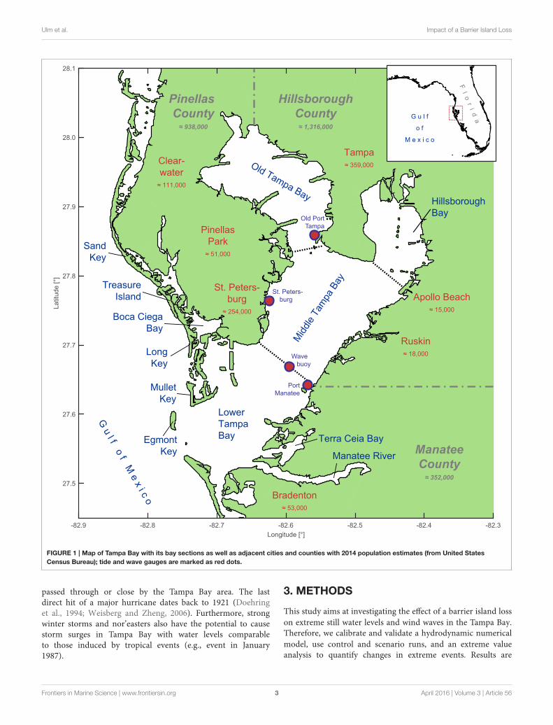
Tampa Bay is an estuary located at Florida’s west-central coastat the Gulf of Mexico. It is surrounded by the countiesPinellas, Hillsborough, andManatee containing large and denselypopulated cities such as St. Petersburg, Clearwater, and Tampa asshown in Figure 1. Several smaller cities are also located close tothe Bay. The cities are heavily developed along the shoreline withresidential, commercial, and industrial infrastructure. Overall thethree counties are home of 2.6 million people (2014 estimatesfrom the United States Census Bureau; http://quickfacts.census.gov).
The entire Tampa Bay has a surface of around 1033 km2
(Kunneke and Palik, 1984) and is commonly divided into fourmajor bay segments, also pictured in Figure 1. Old Tampa Bayand Hillsborough Bay are located in the north. Middle TampaBay forms the central region and Lower Tampa Bay connectswith the Gulf of Mexico. Terra Ceia Bay and the tidal reach ofthe Manatee River are two segments in the south. Boca Ciega Baycreates the western coast of St. Petersburg and is protected by theislands Long Key, Treasure Island, and Sand Key. Egmont Keyis located south of Mullet Key at the mouth of Tampa Bay, theconnection between Lower Tampa Bay and the Gulf of Mexico.The alongshore profile of Egmont Key blocksmore than a third ofthe Bay’s mouth with a length of 3 km perpendicular to the outletdirection. Egmont Key arose from sediments provided by theTampa Bay which were partially deposited in the ebb-tidal deltaof the estuary due to the common action of tides and waves. Theentire sediment complex below the barrier island extents 10 kminto the Gulf of Mexico (Stott and Davis, 2003). The first detailedsurvey of Egmont Key dates back to 1877 and changes in shapeand size were already documented at that time (see Figure 5 inStott and Davis, 2003). Today the U.S. Army Corps of Engineers(USACE) tries to hinder the erosion of Egmont Key with beachnourishment measures which currently help maintaining theshape of the island.
Tampa Bay’s connection to the Gulf of Mexico is narrowed byEgmont Key. A 30 m deep passage north of the island is used asthe entrance to the main shipping channel. Overall Tampa Bay ischaracterized by shallow waters with an average depth of 3.5 m.Exceptions are, beside the mentioned outlet, the harbors anddredged shipping lanes to the ports of St. Petersburg, Tampa, andPort Manatee (Goodwin and Michaelis, 1984). The tidal regimeis mixed semi-diurnal.
Like the entire Gulf region, the Tampa Bay area is threatenedby tropical storms originating from the Atlantic Ocean orCaribbean Sea. In the past decades some severe tropical cyclonesoccurred in the eastern Gulf of Mexico but none directly
Frontiers in Marine Science | www.frontiersin.org 2 April 2016 | Volume 3 | Article 56
Ulm et al. Impact of a Barrier Island Loss
Longitude [°]
-82.9 -82.8 -82.7 -82.6 -82.5 -82.4 -82.3
La
titu
de
[°]
27.5
27.6
27.7
27.8
27.9
28.0
28.1
Old Tampa Bay
Mid
dle
Tam
pa B
ay
St. Peters-
burg
≈ 254,000
Tampa
≈ 359,000
Hillsborough
Bay
Lower
Tampa
Bay
Manatee River
Boca Ciega
Bay
Egmont
Key
Bradenton
≈ 53,000
Clear-
water
≈ 111,000
Pinellas
Park
≈ 51,000
G u
l f o f M
e x i c o
Terra Ceia Bay
Sand
Key
Long
Key
Treasure
Island
Mullet
Key
Hillsborough
County ≈ 1,316,000
Pinellas
County ≈ 938,000
Manatee
County ≈ 352,000
Apollo Beach
≈ 15,000
Ruskin
≈ 18,000
Old Port
Tampa
St. Peters-
burg
Port
Manatee
Wave
buoy
F l o
r i d aG u l f
o f
M e x i c o
FIGURE 1 | Map of Tampa Bay with its bay sections as well as adjacent cities and counties with 2014 population estimates (from United States
Census Bureau); tide and wave gauges are marked as red dots.
passed through or close by the Tampa Bay area. The lastdirect hit of a major hurricane dates back to 1921 (Doehringet al., 1994; Weisberg and Zheng, 2006). Furthermore, strongwinter storms and nor’easters also have the potential to causestorm surges in Tampa Bay with water levels comparableto those induced by tropical events (e.g., event in January1987).
3. METHODS
This study aims at investigating the effect of a barrier island loss
on extreme still water levels and wind waves in the Tampa Bay.Therefore, we calibrate and validate a hydrodynamic numerical
model, use control and scenario runs, and an extreme valueanalysis to quantify changes in extreme events. Results are
Frontiers in Marine Science | www.frontiersin.org 3 April 2016 | Volume 3 | Article 56
Ulm et al. Impact of a Barrier Island Loss
presented as changes in return levels (of still water and significantwave height) due to the modeled barrier island loss.
3.1. Numerical Model SetupThe investigations are based on numerical model experimentsrequiring hydrodynamic forces at the open boundaries as input.The tides and waves within Tampa Bay are primarily fromthe Gulf of Mexico but there is no continuous water levelhindcast available covering the period under investigation orthe investigated area. This is why we set up a two-dimensional,depth-averaged, barotropic tide surge model covering the entireGulf of Mexico, hereafter referred to as Gulf Model. Thislarge-scale model is intended to provide water level boundaryconditions for a higher resolution model of the main studyarea covering the entire Tampa Bay, hereafter referred to asBay Model. This setup enables us to fully describe all relevanthydrodynamic processes adjacent to and within Tampa Bay.Detailed information and references for all data sets describedbelow are summarized in Table 1. The numerical model setup isbriefly summed up in Table 2.
The models are set up and computed using the open sourcemodeling suite Delft3D, provided by Deltares (Lesser et al., 2004).The spatial discretization is achieved using curvilinear grids,shown in Figure 2. In the Gulf Model, cell sizes between 30 and3 km are used. The grid resolution increases from west to eastin order to provide the most accurate results in front of TampaBay without spending too much computation time. In the BayModel, cell sizes range from 400 to 150 m, depending on location
and grid curvature. Bothmodels are configured within a coastlineprovided by the Gulf of Mexico Coastal Ocean Observing System(GCOOS) with a spatially consistent resolution of 60 m.
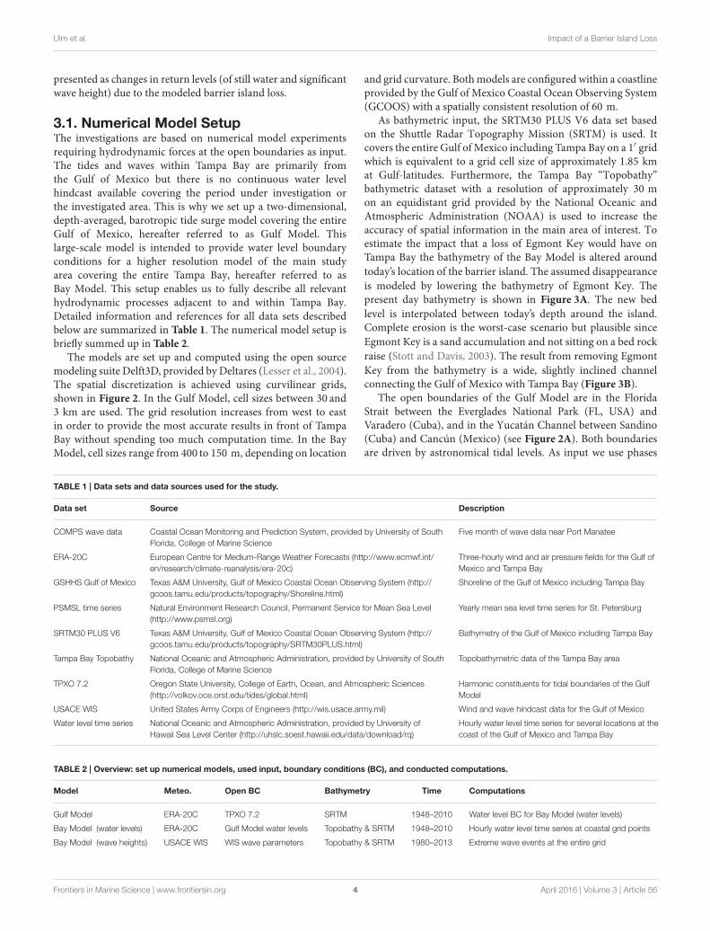
As bathymetric input, the SRTM30 PLUS V6 data set basedon the Shuttle Radar Topography Mission (SRTM) is used. Itcovers the entire Gulf ofMexico including Tampa Bay on a 1′ gridwhich is equivalent to a grid cell size of approximately 1.85 kmat Gulf-latitudes. Furthermore, the Tampa Bay “Topobathy”bathymetric dataset with a resolution of approximately 30 mon an equidistant grid provided by the National Oceanic andAtmospheric Administration (NOAA) is used to increase theaccuracy of spatial information in the main area of interest. Toestimate the impact that a loss of Egmont Key would have onTampa Bay the bathymetry of the Bay Model is altered around
today’s location of the barrier island. The assumed disappearance
is modeled by lowering the bathymetry of Egmont Key. Thepresent day bathymetry is shown in Figure 3A. The new bed
level is interpolated between today’s depth around the island.Complete erosion is the worst-case scenario but plausible since
Egmont Key is a sand accumulation and not sitting on a bed rock
raise (Stott and Davis, 2003). The result from removing Egmont
Key from the bathymetry is a wide, slightly inclined channelconnecting the Gulf of Mexico with Tampa Bay (Figure 3B).
The open boundaries of the Gulf Model are in the FloridaStrait between the Everglades National Park (FL, USA) andVaradero (Cuba), and in the Yucatán Channel between Sandino(Cuba) and Cancún (Mexico) (see Figure 2A). Both boundariesare driven by astronomical tidal levels. As input we use phases
TABLE 1 | Data sets and data sources used for the study.
Data set Source Description
COMPS wave data Coastal Ocean Monitoring and Prediction System, provided by University of South
Florida, College of Marine Science
Five month of wave data near Port Manatee
ERA-20C European Centre for Medium-Range Weather Forecasts (http://www.ecmwf.int/
en/research/climate-reanalysis/era-20c)
Three-hourly wind and air pressure fields for the Gulf of
Mexico and Tampa Bay
GSHHS Gulf of Mexico Texas A&M University, Gulf of Mexico Coastal Ocean Observing System (http://
gcoos.tamu.edu/products/topography/Shoreline.html)
Shoreline of the Gulf of Mexico including Tampa Bay
PSMSL time series Natural Environment Research Council, Permanent Service for Mean Sea Level
(http://www.psmsl.org)
Yearly mean sea level time series for St. Petersburg
SRTM30 PLUS V6 Texas A&M University, Gulf of Mexico Coastal Ocean Observing System (http://
gcoos.tamu.edu/products/topography/SRTM30PLUS.html)
Bathymetry of the Gulf of Mexico including Tampa Bay
Tampa Bay Topobathy National Oceanic and Atmospheric Administration, provided by University of South
Florida, College of Marine Science
Topobathymetric data of the Tampa Bay area
TPXO 7.2 Oregon State University, College of Earth, Ocean, and Atmospheric Sciences
(http://volkov.oce.orst.edu/tides/global.html)
Harmonic constituents for tidal boundaries of the Gulf
Model
USACE WIS United States Army Corps of Engineers (http://wis.usace.army.mil) Wind and wave hindcast data for the Gulf of Mexico
Water level time series National Oceanic and Atmospheric Administration, provided by University of
Hawaii Sea Level Center (http://uhslc.soest.hawaii.edu/data/download/rq)
Hourly water level time series for several locations at the
coast of the Gulf of Mexico and Tampa Bay
TABLE 2 | Overview: set up numerical models, used input, boundary conditions (BC), and conducted computations.
Model Meteo. Open BC Bathymetry Time Computations
Gulf Model ERA-20C TPXO 7.2 SRTM 1948–2010 Water level BC for Bay Model (water levels)
Bay Model (water levels) ERA-20C Gulf Model water levels Topobathy & SRTM 1948–2010 Hourly water level time series at coastal grid points
Bay Model (wave heights) USACE WIS WIS wave parameters Topobathy & SRTM 1980–2013 Extreme wave events at the entire grid
Frontiers in Marine Science | www.frontiersin.org 4 April 2016 | Volume 3 | Article 56

Ulm et al. Impact of a Barrier Island Loss
-98 -96 -94 -92 -90 -88 -86 -84 -82 -80
Longitude [°]
15
17
19
21
23
25
27
29
31
33
La
titu
de
[°]
Gulf Model grid
-83.2 -83.0 -82.8 -82.6 -82.4
Longitude [°]
27.3
27.5
27.7
27.9
28.1
La
titu
de
[°]
Bay Model grid
(A1)
(A2)
(B1)(B)
A B
FIGURE 2 | Curvilinear grids (blue) and shoreline (red) used for the Gulf Model (A) and for the Bay Model (B). For clearness, the grids in this figure appear
with a coarser resolution than used for the simulation. The Gulf Model grid (A) is actually two times higher resolved, the Bay Model grid (B) three times higher. Black
lines indicate the model boundaries of the Gulf Model in the Yucatán Channel (A1), in the Florida Strait (A2) as well as the boundary toward the Gulf of Mexico in the
Bay Model (B1).
Present-day bathymetry
-82.85 -82.80 -82.75 -82.70 -82.65 -82.60
Longitude [°]
27.50
27.55
27.60
27.65
27.70
27.75
La
titu
de
[°]
-5 0 5 10 15 20 25
Scenario bathymetry
-82.85 -82.80 -82.75 -82.70 -82.65 -82.60
Longitude [°]
27.50
27.55
27.60
27.65
27.70
27.75
La
titu
de
[°]
Depth [m]
A B
FIGURE 3 | Unchanged control run bathymetry (A) and scenario bathymetry without Egmont Key (B).
and amplitudes of the main tidal constituents obtained from theglobal ocean tides model TPXO 7.2, provided by the Collegeof Earth, Ocean, and Atmospheric Sciences at the Oregon State
University. The Gulf Model is used to model the transition ofthe tidal components from the Atlantic into the Gulf of Mexicoocean basin. TPXO 7.2 contains 13 harmonic constituents (M2,
Frontiers in Marine Science | www.frontiersin.org 5 April 2016 | Volume 3 | Article 56

Ulm et al. Impact of a Barrier Island Loss
S2, N2, K2, K1, O1, P1, Q1, MF, MM, M4, MS4, MN4) for eachpoint on a global grid with a 0.25° resolution. Tidal boundaryconditions are derived by interpolating the nearest TPXO 7.2gridded information on the models open boundaries. Withinboth models, tidal forces acting on the entire body of water arealso considered including eleven semi-diurnal, diurnal, and longperiod tidal constituents (M2, S2, N2, K2, K1, O1, P1, Q1, MF,MM, SSA). The water levels from the Gulf Model force the BayModel at the boundary indicated in Figure 2B.
The models are additionally forced with spatially varyingmeteorological data (i.e., wind and atmospheric pressure fields)covering the entire model domain. We use data from the ERA-20C reanalysis provided by the European Centre for Medium-Range Weather Forecasts (ECMWF). The reanalysis data coversthe period 1900–2010 and has a temporal resolution of 3 hand a spatial resolution of 1° on a global grid. For waterlevel computations the years 1948–2010 have been chosen sinceobservations at the gauge St. Petersburg (providing the longestrecord for the region) are limited to this period. The usedreanalysis data are limited to the description of meteorologicalconditions at a supra-regional level due to the temporal andspatial resolution. Local and regional anomalies, e.g., in theproximity of tropical cyclones, are represented with little detail,but at the same time no major hurricane passed directly overTampa Bay within the model time frame making the applicationof ERA-20C wind and pressure fields more suitable for theinvestigation area. The availability of the wave input from theUSACE Wave Information Studies (WIS) project is restricted tothe period 1980–2013. Therefore, wind data are also taken fromthis data base for the wave simulation as well as wave height,direction, amplitude, and spread information. The WIS hindcastis available at grid points along the entire U.S. coast. Three pointsclose to the mouth of Tampa Bay are used to force the BayModel.Between these points the boundary conditions are interpolatedlinearly.
In the Bay Model, mean sea level (MSL) changes are alsoconsidered using the Permanent Service for Mean Sea Level(PSMSL) time series of St. Petersburg obtained from the BritishNatural Environment Research Council. Since the computationsfor each year of the simulation time are run separately to handlethe large output data, theMSL is adjusted according to the annualchange in the PSMSL time series.
3.2. Numerical Model Calibration andValidationThe overall aim of this paper is to assess changes in bothextreme still water levels along the coastline and wave heights asconsequence of the loss of Egmont Key. Simplified, simulationsof water level and wave height variables are conducted separatelyenabling to evaluate the contribution of each component to atotal water level independently. Tides and wind set up off themouth of Tampa Bay are extracted from three grid points ofthe Gulf Model. Bay Model water level time series are extractedat about 800 grid points along the coastline in intervals ofapproximately 1 km and wave parameters are extracted from theentire grid since we expect major changes off the coastline, withpotential effects on navigation during extreme events.
In hydrological modeling various efficiency criteria are used todescribe the goodness of model calibration (Krause et al., 2005).Here we use the coefficient of determination (r2) and the rootmean squared error (RMSE). The coefficient of determinationis defined as the squared value of the coefficient of correlation(Krause et al., 2005). The coefficient is calculated with observed(xo) and simulated (xs) water level time series, each with kcorresponding values:
r2 =
∑ki=1 (xsi − x̄s) (xoi − x̄o)
√
∑ki=1 (xoi − x̄o)
2√
∑ki=1 (xsi − x̄s)
2
2
(1)
A value of r2 = 1 [-] denotes that both time series, observed andsimulated, are identical. A value of r2 = 0 [-] indicates that thereis no correlation (Krause et al., 2005). The root mean squarederror is calculated using the time series mentioned above with kvalues:
RMSE =
√
√
√
√
1
k
k∑
i=1
(xoi − xsi)2 (2)
The calibration of the models is done stepwise by adjusting themodeled water levels to recorded data at specific locations usingthe introduced efficiency criteria. The Gulf Model is calibratedfirst since this model provides the input of the Bay Model.The tide gauge of Clearwater, located approximately 45 kmnorth of the mouth of Tampa Bay is used as reference for thecalibration. Furthermore, three tide gauges at the U.S. Gulf coastare used to check the model performance including Apalachicola(Florida), Grand Isle (Louisiana), and Galveston Pier (Texas).All time series are obtained from the NOAA tide gauge database.
The Gulf Model’s parameters and boundary conditions areadjusted in two steps. In the first step a calibration is done byvarying the Manning’s roughness coefficients (n values). In thesecond step the harmonic constituents at the open boundaries ofthe Gulf Model are adjusted. At the beginning of the calibrationexercise, the n values are very uncertain. The Gulf Model iscalibrated by iteratively computing the model with varyingManning’s n values in the range 0.02 ≤ n ≤ 0.04 s/m1/3
and comparing the computation results (using the test statisticsdescribed above) with the tidal predictions from the tide gaugeClearwater provided by NOAA. The calibration consists ofmultiple simulations over 1 month periods, in each case with aspin-up time of 2 weeks.
A Manning’s roughness of n = 0.035 s/m1/3 showsthe smallest achievable error with unmodified harmonicconstituents. Using this roughness significantly increases theaccuracy of the model results but deviations of up to 10 cmare still present. To reduce the remaining differences betweensimulated and observed data the second calibration step isconducted. The input of amplitudes and phases for eachboundary point at the Florida Strait and the Yucatán Channel iscorrected by adjusting the input amplitudes and phases in orderto minimize the error. Similar to the roughness calibration this isdone iteratively.
Frontiers in Marine Science | www.frontiersin.org 6 April 2016 | Volume 3 | Article 56

Ulm et al. Impact of a Barrier Island Loss
Tidal predictions provided by NOAA are separated intotheir underlying constituents and individually compared to thecorresponding constituents from the simulation results. The tidalanalyses are performed with the T_TIDE tool by Pawlowiczet al. (2002). The component breakdown shows which tidalcomponents have the largest influence on the errors. Errorsare reduced by the adjustment of corresponding constituents(amplitudes and phases) at the boundaries. A linear dependencebetween constituents at the gauge site and at the boundariesis assumed for the iterative calibration process. This approachdisregards that tidal oscillations at the gauge are a combination oftidal oscillations at the boundaries and tides originating from theGulf ofMexico but yet leads to a fast convergence of observed andsimulated constituents. After calibration the correction factorsfor the amplitude famp are in a range of 0.9 ≤ famp ≤ 1.4 [-] andthe addends for the phase fpha in the range of −60° ≤ fpha ≤ 15°respectively. All correction factors and addends are presented inTable 3.
After calibration the comparison of full time series atgauge Clearwater results in a coefficient of determination ofr2 = 0.96 [-], showing that the model reliably reproducesobserved water levels at this site, close to the mouth of TampaBay. The RMSE calculation shows errors of 5.1 cm for tidal highwater levels and 5.7 cm for tidal low water levels. The observedmean tidal range at gauge Clearwater is 58 cm. Overall the modeltends to overestimate the minor high and low waters of the mixedsemi-diurnal tide cycle, whereas higher high waters are computedmore reliably enabling to simulate extremes properly.
The Bay Model is forced with the Gulf Model water levelsand also calibrated. The calibration of the Bay Model is limitedto the adjustment of the Manning’s roughness coefficient n. Theinput boundary condition has been computed by the calibratedGulf Model and therefore should not be changed. Tampa Bay ismonitored by several hydrological andmeteorological measuringstations. Three of four active tide gauges within the estuary areunaffected by inflowing rivers and are used here for calibration,validation, and bias correction of the Bay Model. These stationsare located at the port of St. Petersburg in the west of thebay, at Port Manatee in the south-east, and at Old Port Tampain the north (see Figure 1). The official tide predictions forthese gauges, provided by NOAA, are used as reference. Theroughness calibration is conducted in the same way the GulfModel has been calibrated. The iterative test considers valuesin the range of 0.02 ≤ n ≤ 0.036 s/m1/3. The best fit ofsimulated time series against observed time series, regardingRMSE and coefficient of determination, is achieved by usinga Manning’s roughness coefficient of n = 0.022 s/m1/3. Thesmaller coefficient, compared to the Gulf Model’s roughness, isattributable to the significantly higher resolution of the seafloortopography in the Bay. The rather coarse resolution of the Gulf
bathymetry only allows a smoothed seafloor in the Gulf Model.Geometric features smaller than the bathymetry resolution haveto be added artificially by increasing the roughness. The BayModel’s bathymetry already depicts most of these features.Therefore, the calibration leads to a smaller roughness coefficient.The efficiency criteria after Krause et al. (2005) described aboveare also calculated for the Bay Model calibration results. RMSEand r2 differ from gauge to gauge within Tampa Bay. Regardingtidal high water levels the RMSE does not exceed 4 cm; thecoefficient of determination spans 0.92 ≤ r2 ≤ 0.95 [-].The comparison of full time series also shows an RMSE ofapproximately 4 cm and r2 ≥ 0.95 [-] for all three gauges.
The wave simulations are conducted using the calibratedwater level model of the Bay. A validation run (focusing onthe significant wave height) has been performed indicating thatthe model reproduces large wave events well for the simulatedperiod using one available buoy data set of the Coastal OceanMonitoring and Prediction System (COMPS). The buoy data wasrecorded at the border of Middle and Lower Tampa Bay (seeFigure 1) covering 5 months (April through August 2012) withhourly wave parameters. Several events from this period havebeen simulated. The model tends to underestimate small waveheights. With focus on the three largest events a comparisonbetween simulated and observed significant wave heights givesan RMSE of 12 cm and r2 = 0.83 [-] where absolute valuesrange from 86 to 91 cm. The largest event shows a deviation of3 cm in significant wave height. Based on the USACE WIS dataonly events larger than the tested wave heights are simulated forthe comparison between control and scenario run. Therefore,the model can be used for the simulations disregarding thedeficiencies in estimating small wave heights. Regarding waveperiods the model shows peak periods of approximately 3 s forthe highest events at the location of the wave buoy. Due to largegaps in the wave period record a validation of this parametercould not be conducted.
3.3. Statistical model setup3.3.1. Pre-processingThe numerical model is used to simulate multi-decadal waterlevel and wind wave time series which are required for reliableextreme value analysis (EVA) of both variables. Extreme waterlevels are assessed at individual grid points along the entireTampa Bay coastline. The wave simulations are used to estimatereturn wave heights for the entire grid. In both cases, simulationsare performed using (A) a current state bathymetry (control run)and (B) a bathymetry where Egmont Key is removed (scenariorun; see Figure 3). Both water level simulations consider the sametime period of 63 years (1948–2010) and the same hydrodynamicand meteorological boundary conditions. The wave simulationsare only conducted for extreme events, since a continuous
TABLE 3 | Factors famp and addends fpha used to correct the Gulf Model input amplitudes and phases.
TPXO constituents M2 S2 N2 K2 K1 O1 P1 Q1 MF MM M4 MS4 MN4
famp 1.4 1.0 1.0 0.9 1.05 1.05 1.1 1.0 1.0 1.0 1.0 1.0 1.0
fpha −15 15 0 0 0 0 0 0 0 0 −60 0 0
Frontiers in Marine Science | www.frontiersin.org 7 April 2016 | Volume 3 | Article 56
Ulm et al. Impact of a Barrier Island Loss
simulation of several consecutive years would be computationallymuch more expensive without adding new relevant informationon extremes. Furthermore, the available wave data used as inputat the open boundaries is event based (not continuous) andcovers the period 1980–2013. The results from the differentmodel runs are used for the EVA.
A fundamental assumption for EVA is that time series arestationary and that events are independent (Coles, 2001; Arnset al., 2013). This is why linear detrending has been applied to alltime series (simulated and observed) in order to account for thefirst criterion. To comply with the second criterion a declusteringprocedure has been applied to the data ensuring that the sampleconsists of independent events. The declustering procedure isconducted as follows: at first all peaks within the simulated anddetrended hourly water level time series are selected andmatchedwith the corresponding peaks in the detrended observation timeseries. Clusters are detected by identifying peaks that occurredwithin 6 h. A simple comparison of two neighboring peaks thatfulfill the 6-h-criterion allows discarding the smaller one sincethis peak is assumed to be not independent of the larger one.Finally, only the largest peak of a tidal high water period is usedfor the EVA (Zachary et al., 1998).
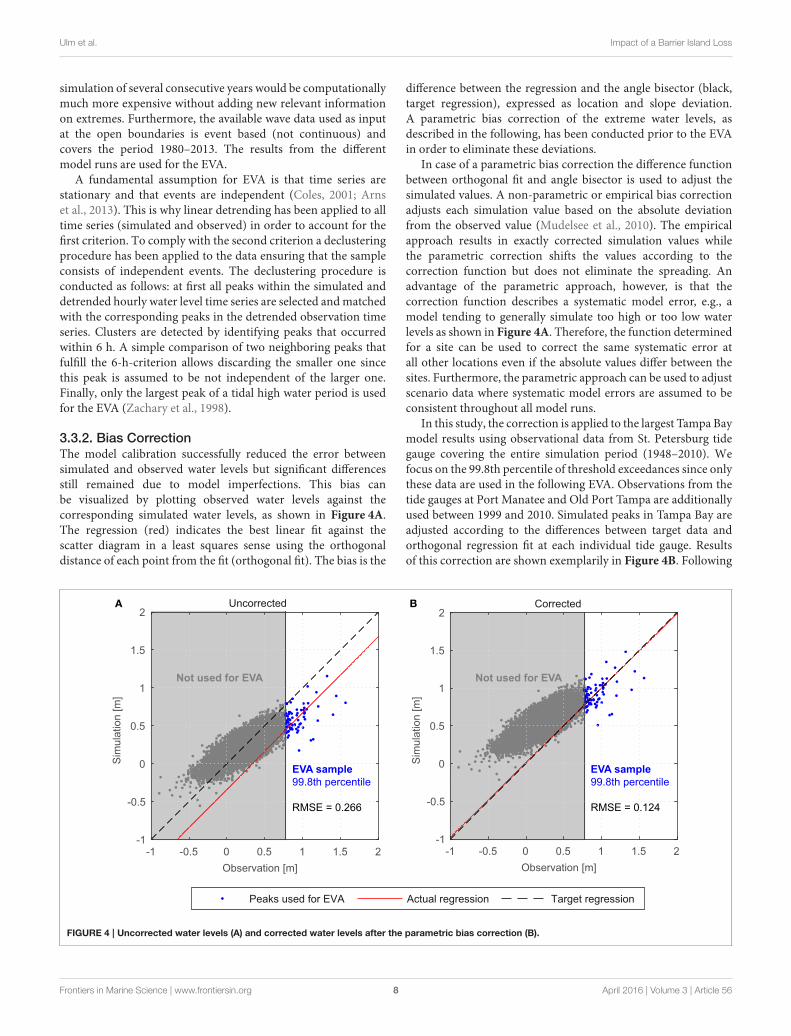
3.3.2. Bias CorrectionThe model calibration successfully reduced the error betweensimulated and observed water levels but significant differencesstill remained due to model imperfections. This bias canbe visualized by plotting observed water levels against thecorresponding simulated water levels, as shown in Figure 4A.The regression (red) indicates the best linear fit against thescatter diagram in a least squares sense using the orthogonaldistance of each point from the fit (orthogonal fit). The bias is the
difference between the regression and the angle bisector (black,target regression), expressed as location and slope deviation.A parametric bias correction of the extreme water levels, asdescribed in the following, has been conducted prior to the EVAin order to eliminate these deviations.
In case of a parametric bias correction the difference functionbetween orthogonal fit and angle bisector is used to adjust thesimulated values. A non-parametric or empirical bias correctionadjusts each simulation value based on the absolute deviationfrom the observed value (Mudelsee et al., 2010). The empiricalapproach results in exactly corrected simulation values whilethe parametric correction shifts the values according to thecorrection function but does not eliminate the spreading. Anadvantage of the parametric approach, however, is that thecorrection function describes a systematic model error, e.g., amodel tending to generally simulate too high or too low waterlevels as shown in Figure 4A. Therefore, the function determinedfor a site can be used to correct the same systematic error atall other locations even if the absolute values differ between thesites. Furthermore, the parametric approach can be used to adjustscenario data where systematic model errors are assumed to beconsistent throughout all model runs.
In this study, the correction is applied to the largest Tampa Baymodel results using observational data from St. Petersburg tidegauge covering the entire simulation period (1948–2010). Wefocus on the 99.8th percentile of threshold exceedances since onlythese data are used in the following EVA. Observations from thetide gauges at Port Manatee and Old Port Tampa are additionallyused between 1999 and 2010. Simulated peaks in Tampa Bay areadjusted according to the differences between target data andorthogonal regression fit at each individual tide gauge. Resultsof this correction are shown exemplarily in Figure 4B. Following
Uncorrected
-1 -0.5 0 0.5 1 1.5 2
Observation [m]
-1
-0.5
0
0.5
1
1.5
2
Sim
ula
tio
n [m
]
Corrected
-1 -0.5 0 0.5 1 1.5 2
Observation [m]
-1
-0.5
0
0.5
1
1.5
2
Sim
ula
tio
n [m
]
Peaks used for EVA Actual regression Target regression
Not used for EVA Not used for EVA
EVA sample
99.8th percentile
RMSE = 0.266
EVA sample
99.8th percentile
RMSE = 0.124
A B
FIGURE 4 | Uncorrected water levels (A) and corrected water levels after the parametric bias correction (B).
Frontiers in Marine Science | www.frontiersin.org 8 April 2016 | Volume 3 | Article 56

Ulm et al. Impact of a Barrier Island Loss
this procedure, data sets at all ungauged grid points of theBay Model are corrected using the correction factors estimatedat the gauged sites. For the years 1999–2010, in which factorsfor all three gauges are available, an inverse distance weightingapproach is used to interpolate the factors to ungauged locationsalong the entire Tampa Bay coastline. It is assumed that the biasmainly originates from model limitations, like the discretizationof wind data or seafloor topography approximations. Therefore,the correction is also applied to the scenario run. Correctedscenario water levels are obtained by calculating the differencesbetween uncorrected control and scenario run water levels andthen adding them to the corrected control run water levels.
The wave control run has not been adjusted as the availablewave data required as input for developing a bias correction onlycovers 5 months with only one extreme event on record. Thus, areliable correction cannot be derived. In our numerical sensitivitystudy, we focus on changes in wave heights as consequence of apotential loss of Egmont Key. The overall aim of this assessmentis to estimate relative changes in wave heights. Based on ourvalidation we assume that the model is able to capture thesechanges reliably.
3.3.3. Return Level AssessmentThe return level assessment is conducted with both controlrun and scenario run water level data at individual grid pointsalong the Tampa Bay coastline and with the correspondingwave simulations with the intention to estimate the impact ofthe disappearing of Egmont Key. Two extreme value analysisapproaches are tested prior to the final assessment, i.e., the BockMaxima (BM) method using the Generalized Extreme ValueDistribution (GEV) and the Peak-over-threshold (POT) methodwith the Generalized Pareto Distribution (GPD).
The BM sampling approach considers the r largest eventswithin a specific time frame, e.g., the three highest water levelsof each year. This yields a sample of events which allows anestimation of return water levels by fitting the GEV to the sample.The GEV unifies three fundamental extreme value distributionsnamely the Gumbel, Fréchet, and Weibull and is defined inEquation 3 with the location parameter−∞ < µ < ∞, the scaleparameter σ > 0, the shape parameter −∞ < ξ < ∞, and theBM values z (Coles, 2001):
GEV = exp
{
−
[
1+ ξ
(
z − µ
σ
)]−1/ξ}
(3)
The POT sampling approach considers all values that exceeda defined threshold u, e.g., the 0.5% largest values of a recordalso referred to as the 99.5th percentile. The GPD is related tothis sampling method and also couples various extreme valuedistributions. It is defined as
GPD = 1−
(
1+ξ · z
σ + ξ · (u− µ)
)−1/ξ
(4)
where µ, σ , ξ , and z denote parameters and values as above(Coles, 2001).
The BM method has been tested with r ∈ {1, 2, 3} valuesper year and the POT approach with the 99.6, 99.7, and 99.8th
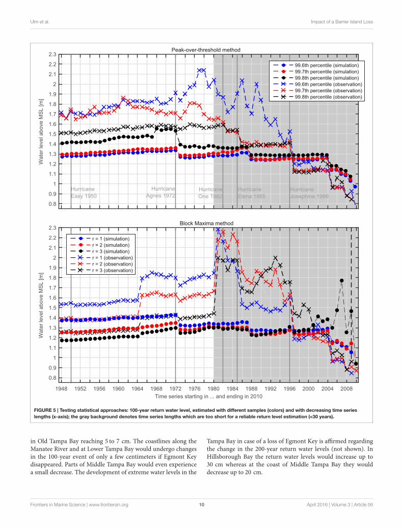
percentile of threshold exceedances. Both methods have beenapplied to subsets of observed and simulated time series of thetide gauge of St. Petersburg. The 100-year return water levelhas been estimated with both methods and different extremevalue model setups using varying time series lengths. The resultsare shown in Figure 5 indicating that the POT approach withthe 99.8th percentile yields the most robust results. Comparedto other approaches, these estimates are among the smallestvariances of all return levels considering different time serieslengths (within a range of 10 cm). The gray shade in Figure 5
denotes time series lengths that are too short for a reliable 100-year return level estimation. Therefore, the results within andclose to the shade vary heavily. With longer time series (especiallystarting between 1948 and 1964) the results are more robust, evenwhen very large events (often associated with tropical cyclones)are excluded from the return level assessment (e.g., HurricaneEasy, 1950). Furthermore, this method with the 99.8th percentilesubset only causes small differences of approximately 10 cmbetween return levels estimated from the observed and from thesimulated time series using the longest period available. OtherEVA model setups yield differences of up to 40 cm. Remainingsmall deviations are assumed to be negligible as we aim atinvestigating the changes induced by the vanishing of EgmontKey and deviations are caused by consistent model deficienciesthat affect control and scenario runs alike.
Frequencies and magnitudes of extreme wave heights areestimated using the same approach as described above. However,in that case we use the 99.5th percentile of all events ofthe USACE WIS database. These selected extreme events aresimulated individually using the control run and scenariobathymetries.
4. RESULTS
4.1. Return Water LevelsExtreme water levels are assessed for different return periodsincluding the 5-, 25-, 50-, 100-, and 200-year events. Thus, thereturn period estimation does not exceed 3 to 4 times the lengthof the underlying time series. The latter limit is recommendede.g., by Pugh (2004). The differences in return water levelsare visualized in Figures 6, 7 for the 25- and 100-year events,respectively. The return water levels are only used for estimatingthe differences a loss of Egmont Key would cause.
A comparison of Figures 6, 7 indicates the overalldevelopment of the results. Changes in water levels withreturn periods shorter than 100 years appear to have a spatiallydifferent characteristic compared to those with return periodsgreater than or equal to 100 years. At shorter return periods,increases can be found along the entire Tampa Bay coastlinewith significant changes in Hillsborough Bay and Old TampaBay. For a return period of 25 years, increases between 3 and5 cm are found. At the tidal reach of the Manatee River and thecoastline of Lower Tampa Bay, close to the mouth of the estuary,increases are in the order of 2 to 3 cm. Middle Tampa Bay is notaffected. Regarding return periods of 100 years or more, largestreturn water level increases are found along Hillsborough Bay.Water levels increase by up to 15 cm. There are also changes
Frontiers in Marine Science | www.frontiersin.org 9 April 2016 | Volume 3 | Article 56
Ulm et al. Impact of a Barrier Island Loss
Time series starting in ... and ending in 2010
1948 1952 1956 1960 1964 1968 1972 1976 1980 1984 1988 1992 1996 2000 2004 2008
Wa
ter
leve
l a
bo
ve
MS
L [m
]
0.8
0.9
1
1.1
1.2
1.3
1.4
1.5
1.6
1.7
1.8
1.9
2
2.1
2.2
2.3Block Maxima method
r = 1 (simulation)
r = 2 (simulation)
r = 3 (simulation)
r = 1 (observation)
r = 2 (observation)
r = 3 (observation)
Wa
ter
leve
l a
bo
ve
MS
L [m
]
0.8
0.9
1
1.1
1.2
1.3
1.4
1.5
1.6
1.7
1.8
1.9
2
2.1
2.2
2.3
Hurricane
Easy 1950
Hurricane
Agnes 1972Hurricane
One 1982
Hurricane
Elena 1985
Hurricane
Josephine 1996
Peak-over-threshold method
99.6th percentile (simulation)
99.7th percentile (simulation)
99.8th percentile (simulation)
99.6th percentile (observation)
99.7th percentile (observation)
99.8th percentile (observation)
FIGURE 5 | Testing statistical approaches: 100-year return water level, estimated with different samples (colors) and with decreasing time series
lengths (x-axis); the gray background denotes time series lengths which are too short for a reliable return level estimation (<30 years).
in Old Tampa Bay reaching 5 to 7 cm. The coastlines along theManatee River and at Lower Tampa Bay would undergo changesin the 100-year event of only a few centimeters if Egmont Keydisappeared. Parts of Middle Tampa Bay would even experiencea small decrease. The development of extreme water levels in the
Tampa Bay in case of a loss of Egmont Key is affirmed regardingthe change in the 200-year return water levels (not shown). InHillsborough Bay the return water levels would increase up to30 cm whereas at the coast of Middle Tampa Bay they woulddecrease up to 20 cm.
Frontiers in Marine Science | www.frontiersin.org 10 April 2016 | Volume 3 | Article 56

Ulm et al. Impact of a Barrier Island Loss
-82.9 -82.8 -82.7 -82.6 -82.5 Longitude [°]
27.3
27.4
27.5
27.6
27.7
27.8
27.9
La
titu
de
[°]
Change in 25-year return water levels [m]
-0.10
-0.05
0
0.05
0.10
0.15
≈ 5 cm
≈ 5 cm
≈ 3 cm
≈ 2 cm
≈ 0 cm
FIGURE 6 | Change in 25-year return water levels for available grid
points along the Tampa Bay and Gulf coastline.
The return level assessment reveals that Egmont Key has asignificant reducing influence on extreme water levels in theTampa Bay. The northern parts of the estuary are protected bythe barrier island and would be affected negatively by a loss ofthe barrier island. Even the smaller but more frequent stormsurge events would increase along large parts of the Tampa Baycoastline.
In addition to the EVA results, differences in maximum waterlevels (scenario to control run) along the coast as well as relativeincreases have been calculated (Figures 8A,B). A loss of EgmontKey leads to water level increases of more than 4 cm in the entireTampa Bay. Manatee River, Lower Tampa Bay, and northernHillsborough Bay water levels increase up to 12 cm which is achange of up to 10%.
4.2. Return Wave HeightsExtreme wave heights are estimated at each grid point includingareas of particular interest like shipping lanes and coastal zones.Overall the wave heights show strong increases around thelocation of today’s Egmont Key in the Gulf of Mexico as well as inLower Tampa Bay. The estimated wave heights for a return periodof 25 years are shown in Figure 9. Entire Lower Tampa Bay wouldbe affected with increases of mostly 0.4 to 1.0 m in areas withoutbathymetric changes. Close to today’s location of Egmont Key,where the bathymetry has been changed, increases range from1.3 to 1.7 m. In contrast,Middle Tampa Bay only shows increases
-82.9 -82.8 -82.7 -82.6 -82.5 Longitude [°]
27.3
27.4
27.5
27.6
27.7
27.8
27.9
La
titu
de
[°]
Change in 100-year return water levels [m]
-0.10
-0.05
0
0.05
0.10
0.15
up to
15 cm
-5 to
-10 cm
5 to 7 cm
≈ 5 cm
≈ 4 cm
FIGURE 7 | Change in 100-year return water levels for available grid
points along the Tampa Bay and Gulf coastline.
of a few centimeters along the center line of the estuary and thenorthern parts of Tampa Bay are not affected at all.
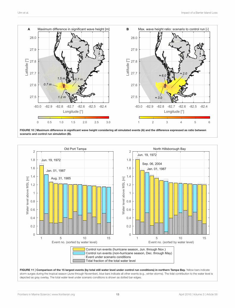
Besides the EVA results, the maximum differences betweenthe control and the scenario run and also the relative increasesof wave heights have been calculated for each grid point (seeFigures 10A,B respectively). Both plots confirm that changesin wave heights are only found in the Lower Tampa Bay area.Maximumdifferences between 1.5 and 2.0 m around the locationof the barrier island could have a significant impact on thenavigability since these increases are a doubling of the today’swave heights in this area. The eastern coast of Lower Tampa Baywould also see significant increases in wave heights (up to 300%).For the city Anna Maria, located on the barrier island south ofEgmont Key, wave height increases of up to 13 cm are found.
Regarding the change in wave period increases are limitedto the area described above. The loss of sheltering and theincreased depth directly behind today’s location of Egmont Keyresult in periods of 9 to 12 s in Lower Tampa Bay under scenarioconditions where control runs show periods of 3 to 5 s. Wavedirections are affected by the removal of Egmont Key as well, butonly in close vicinity to the barrier island.
5. DISCUSSION AND CONCLUSIONS
The simulation of water levels and waves in the Tampa Bay withand without the barrier island Egmont Key shows that the islandprovides significant natural coastal protection. For extreme still
Frontiers in Marine Science | www.frontiersin.org 11 April 2016 | Volume 3 | Article 56

Ulm et al. Impact of a Barrier Island Loss
-82.9 -82.8 -82.7 -82.6 -82.7 Longitude [°]
27.3
27.4
27.5
27.6
27.7
27.8
27.9
La
titu
de
[°]
Max. water level ratio: scenario to control run [-]
0.90
0.92
0.94
0.96
0.98
1.00
1.02
1.04
1.06
1.08
1.10
-82.9 -82.8 -82.7 -82.6 -82.5 Longitude [°]
27.3
27.4
27.5
27.6
27.7
27.8
27.9
La
titu
de
[°]
Difference in maximum coastal water levels [m]
-0.12
-0.08
-0.04
0
0.04
0.08
0.12
4 to 7 cm
up to
12 cm
4 to 5 cm
up to
12 cm
7 to 10 cm
≈ 1.10
1.06 to
1.10
≈ 1.04
≈ 1.06
≈ 1.07
A B
FIGURE 8 | Difference in maximum water levels along the coastline (A) and the difference expressed as ratio between scenario and control run
simulation (B).
Difference in 25-year return wave height [m]
-83.0 -82.9 -82.8 -82.7 -82.6 -82.5 -82.4
Longitude [°]
27.5
27.6
27.7
27.8
27.9
28.0
La
titu
de
[°]
0 0.5 1.0 1.5 2.0
1.7 m 0.4 m
0.5 m
1.0 m
FIGURE 9 | Change in 25-year return wave height for all grid points.
water levels the removal of Egmont Key from the model’sbathymetry yielded higher return water levels in the northernparts of the estuary. The absence of the barrier that blocks about
a third of the mouth of Tampa Bay allows westerly winds togenerate more wind set-up in the estuary. The northern baysections as well as the Manatee River are affected most due to thevery shallow waters and narrow connections to Middle TampaBay that only allow a limited near-ground back flow. The extremewater level increases in the northern bay sections are expected tobe larger than a decimeter in case of a 100-year event which is achange of about 10%. The affected areas are densely populatedand developed with residential, commercial, and industrialinfrastructure close to the waterfront. Smaller events that occurmore frequently (e.g., 25-year return period) are also expected toincrease when Egmont Key disappears. From a coastal protectionperspective, it is thus reasonable to put effort in the maintenanceof Egmont Key since large parts of the adjacent mainland islow-lying and therefore already vulnerable to extreme waterlevels and waves. An increase in extreme events, adding up onthe existing level, would increase the ecological and economicalrisk.
Middle Tampa Bay shows only small increases in 25-yearreturn levels and even a decrease in the 100-year water level. Thiscan primarily be attributed to a change of the shape parameterof the extreme value distribution. In this area, under scenarioconditions, relative increases of smaller events are larger thanthose of the most extreme events. Therefore, the EVA leads tosmaller return levels, especially for longer return periods. Wespeculate that the most extreme events do not increase as muchas the smaller events due to an increased back flow since the
Frontiers in Marine Science | www.frontiersin.org 12 April 2016 | Volume 3 | Article 56
Ulm et al. Impact of a Barrier Island Loss
Max. wave height ratio: scenario to control run [-]
Longitude [°]
-83.0 -82.9 -82.8 -82.7 -82.6 -82.5 -82.4
La
titu
de
[°]
27.5
27.6
27.7
27.8
27.9
28.0
1 2 3 4 5 6
Maximum difference in significant wave height [m]
Longitude [°]
-83.0 -82.9 -82.8 -82.7 -82.6 -82.5 -82.4
La
titu
de
[°]
27.5
27.6
27.7
27.8
27.9
28.0
0 0.5 1.0 1.5 2.0 2.5 3.0
1.5 m 0.7 m
1.2 m
0.7 m
≈ 3.0
≈ 6.0≈ 2.0
A B
FIGURE 10 | Maximum difference in significant wave height considering all simulated events (A) and the difference expressed as ratio between
scenario and control run simulation (B).
1 10 15
Event no. (sorted by water level)
0
0.2
0.4
0.6
0.8
1
1.2
1.4
1.6
1.8
2
Wa
ter
leve
l a
bo
ve
MS
L [m
]
Old Port Tampa
Jun. 19, 1972
Jan. 01, 1987
Aug. 31, 1985
1 10 15
Event no. (sorted by water level)
0
0.2
0.4
0.6
0.8
1
1.2
1.4
1.6
1.8
2
Wa
ter
leve
l a
bo
ve
MS
L [m
]
North Hillsborough Bay
Jun. 19, 1972
Sep. 06, 2004
Jan. 01, 1987
Control run events (hurricane season, Jun. through Nov.)
Control run events (non-hurricane season, Dec. through May)
Event under scenario conditions
Tidal fraction of the total water level
5 5
FIGURE 11 | Comparison of the 15 largest events (by total still water level under control run conditions) in northern Tampa Bay. Yellow bars indicate
storm surges during the tropical season (June through November), blue bars indicate all other events (e.g., winter storms). The tidal contribution to the water level is
depicted as gray overlay. The total water level under scenario conditions is shown as dotted bar edges.
Frontiers in Marine Science | www.frontiersin.org 13 April 2016 | Volume 3 | Article 56
Ulm et al. Impact of a Barrier Island Loss
removal of the barrier island also enlarges the outflow cross-section.
The wave height assessment shows that the potential loss ofEgmont Key has a significant impact on the waves in LowerTampa Bay but overall the influence occurs locally. The effect ofEgmont Key is limited to an area which extends approximately10 km into the Bay, measured from today’s location of the island.Increasing wave heights in this area can be attributed to themissing barrier which today shelters Lower Tampa Bay directly,and to the increased depth around the location of Egmont Key.Areas in the northern Tampa Bay are protected by the shallowwaters of the estuary, which would dissipate most wave energyin case that Egmont Key completely disappears. The very localchange in wave directions is also attributable to the increaseddepth. With the loss of Egmont Key and the increase in waterdepth local shallow water effects like refraction and diffractiondo not appear anymore. Waves from the Gulf of Mexico enterTampa Bay unchanged until the depth limitation decreases waveheights significantly.
The EVA has been conducted without distinguishing betweenevent types. Tampa Bay is located in an area where tropicalcyclones occur during summer and fall months. Therefore,separate analyses of tropical and extra-tropical events wouldbe a reasonable approach, as described e.g., by Haigh et al.(2014). Furthermore, this would be necessary in case that thestudy aims at estimating absolute heights for return periods. Thesimplified method used in this study is feasible since no majortropical cyclone directly hit Tampa Bay within the time period ofinterest. Figure 11 shows that tropical and extra-tropical eventsin Tampa Bay led to similar total still water levels. Possiblechanges from other extreme events that occured beyond theperiod of observation are not considered in this particular studybut could also have an effect on the shape of the underlyingextreme value distribution. Additionally the return levels are onlyused for the A-B-comparison and therefore the chosen simplifiedmethod leads to suitable results.
Figure 11 also shows the tide-surge-ratio of the top events inTampa Bay. Haigh et al. (2010) detected an underestimation forlarge return periods when using direct methods (i.e., conductingan EVA with the total water level signal instead of modeling andexamining tide and surge components separately) in case thatthe tidal component is larger than twice the size of the non-tidalcomponent. In this context, the large contribution of the surge
component to the total still water levels in Tampa Bay confirmsthe applicability of the direct approach.
Regarding the analyzed processes, this study focuses on waterlevels and waves. Changes in estuarine circulations have beenneglected but may also be significantly affected by a loss ofEgmont Key. In particular, changes in the tidal prism, tidalcurrents, exchange circulation and flushing could occur. Thesechanges are associated with alterations in the entire ecosystemand should be investigated in further studies.
Overall the complete removal of Egmont Key is a simplifiedapproach and disregards other morphologic changes inthe barrier island system which would probably occursimultaneously with an erosion of the island extending overseveral decades. Examples are coastline changes in Tampa Bay
or at the Gulf coast near the mouth of the estuary, changes indepth due to sediment displacement, and the impact of sea levelrise. Albeit using a worst-case scenario, the presented resultsshow that Egmont Key significantly alters extreme events inTampa Bay and that a detailed investigation of realistic scenariosis needed. Further studies could include the above-mentionedmorphologic and hydrodynamic changes to improve the results.Furthermore, inundation of the low-lying islands and of themainland during storm surges should be considered. Authoritiesand coastal managers could benefit from the results and usethe findings to develop appropriate protection strategies for theTampa Bay area.
AUTHOR CONTRIBUTIONS
AA, TW, and MU developed the concept. MU set up and ranthe models, analyzed output data, and drafted the paper withthe guidance of AA. SM provided fundamental model data. Allauthors revised and finalized the draft. ML and JJ supervised theresearch project and finally approved the paper.
ACKNOWLEDGMENTS
All analyses presented in this paper were part of the projectThe effect of eroding barrier islands on coastal flood riskand estuarine health (project ID 57052194), supported bythe German Academic Exchange Service (DAAD) with fundsof the German Federal Ministry of Education and Research(BMBF).
REFERENCES
Arns, A., Wahl, T., Haigh, I. D., Jensen, J., and Pattiaratchi, C. (2013).
Estimating extreme water level probabilities: a comparison of the direct
methods and recommendations for best practise. Coast. Eng. 81, 51–66. doi:
10.1016/j.coastaleng.2013.07.003
Coles, S. (2001).An Introduction to Statistical Modeling of Extreme Values. London:
Springer.
Cromwell, J. E. (1973). “Barrier coast distribution: a world survey,” in Barrier
Islands. Benchmark Papers in Geology,Vol. 9, ed M. L. Schwartz, (Stroudsburg,
PA: Douden, Hutchinson, and Ross), 407–408.
Doehring, F., Duedall, I. W., and Williams, J. M. (1994). Florida Hurricanes
and Tropical Storms: 1871-1993: An Historical Survey, Vol. 71 of Technical
Paper. Gainesville, FL: Florida Sea Grant College Program, University of
Florida.
Goodwin, C. R., and Michaelis, D. M. (1984). Appearance and Water Quality of
Turbidity Plumes Produced by Dredging in Tampa Bay, Florida, Vol. 2192 of
United States Geological Survey Water-Supply Paper. Washington: G.P.O.
Haigh, I. D., MacPherson, L. R., Mason, M. S., Wijeratne, E. M. S., Pattiaratchi,
C. B., Crompton, R. P., et al. (2014). Estimating present day extreme water level
exceedance probabilities around the coastline of australia: tropical cyclone-
induced storm surges. Clim. Dyn. 42, 139–157. doi: 10.1007/s00382-012-
1653-0
Haigh, I. D., Nicholls, R., andWells, N. (2010). A comparison of the main methods
for estimating probabilities of extreme still water levels.Coast. Eng. 57, 838–849.
doi: 10.1016/j.coastaleng.2010.04.002
Frontiers in Marine Science | www.frontiersin.org 14 April 2016 | Volume 3 | Article 56
Ulm et al. Impact of a Barrier Island Loss
Krause, P., Boyle, D. P., and Bäse, F. (2005). Comparison of different efficiency
criteria for hydrological model assessment. Adv. Geosci. 5, 89–97. doi:
10.5194/adgeo-5-89-2005
Kunneke, J. T., and Palik, T. F. (1984). Tampa Bay Environmental Atlas, Vol. 85
(15) of Biological Report / Fish and Wildlife Service. Washington, DC: Fish and
Wildlife Service, U.S. Dept. of the Interior.
Lesser, G. R., Roelvink, J. A., van Kester, J. A. T. M., and Stelling, G. S. (2004).
Development and validation of a three-dimensional morphological model.
Coast. Eng. 51, 883–915. doi: 10.1016/j.coastaleng.2004.07.014
List, J. H., and Hansen, M. E. (1992). “The value of barrier islands: 1. Mitigation
of locally-generated wind-wave attack on the mainland,” in Open-File Report
(St. Petersburg, FL: United States Geological Survey), 92–722.
Mudelsee, M., Chirila, D., Deutschländer, T., Döring, C., Haerter, J., Hagemann,
S., et al. (2010). Climate Model Bias Correction und die Deutsche
Anpassungsstrategie. DMGMitteilungen 03/2010, 2–7. doi: 10013/epic.37089
Oertel, G. F. (1985). The barrier island system. Marine Geol. 63, 1–18. doi:
10.1016/0025-3227(85)90077-5
Passeri, D. L., Hagen, S. C., Bilskie, M. V., and Medeiros, S. C. (2015a). On
the significance of incorporating shoreline changes for evaluating coastal
hydrodynamics under sea level rise scenarios.Nat. Hazards 75, 1599–1617. doi:
10.1007/s11069-014-1386-y
Passeri, D. L., Hagen, S. C., Medeiros, S. C., and Bilskie, M. V. (2015b). Impacts of
historic morphology and sea level rise on tidal hydrodynamics in a microtidal
estuary (Grand Bay, Mississippi). Continent. Shelf Res. 111, 150–158. doi:
10.1016/j.csr.2015.08.001
Pawlowicz, R., Beardsley, B., and Lentz, S. (2002). Classical tidal harmonic analysis
including error estimates in MATLAB using T_TIDE. Comput. Geosci. 28,
929–937. doi: 10.1016/S0098-3004(02)00013-4
Pugh, D. (2004). Changing Sea Levels: Effects of Tides, Weather and Climate.
Cambridge: Cambridge University Press.
Stone, G. W., and McBride, R. A. (1998). Louisiana barrier islands
and their importance in wetland protection: forecasting shoreline
change and subsequent response of wave climate. J. Coast. Res. 14,
900–915.
Stone, G. W., Zhang, X., and Sheremet, A. (2005). The role of Barrier Islands,
muddy shelf and reefs in mitigating the wave field along coastal Louisiana. J.
Coast. Res. 44, 40–55. Available online at: http://www.jstor.org/stable/25737048
Stott, J. K., and Davis, R. A. (2003). Geologic development and morphodynamics
of Egmont Key, Florida. Marine Geol. 200, 61–76. doi: 10.1016/S0025-
3227(03)00177-4
Stutz, M. L., and Pilkey, O. H. (2001). A review of global barrier island distribution.
J. Coast. Res. 34, 15–22. Available online at: http://www.jstor.org/stable/
25736270
Weisberg, R. H., and Zheng, L. (2006). Hurricane storm surge simulations for
Tampa Bay. Estuar. Coast 29, 899–913. doi: 10.1007/BF02798649
Zachary, S., Feld, G., Ward, G., and Wolfram, J. (1998). Multivariate extrapolation
in the offshore environment. Appl. Ocean Res. 20, 273–295. doi: 10.1016/S0141-
1187(98)00027-3
Conflict of Interest Statement: The authors declare that the research was
conducted in the absence of any commercial or financial relationships that could
be construed as a potential conflict of interest.
Copyright © 2016 Ulm, Arns, Wahl, Meyers, Luther and Jensen. This is an open-
access article distributed under the terms of the Creative Commons Attribution
License (CC BY). The use, distribution or reproduction in other forums is permitted,
provided the original author(s) or licensor are credited and that the original
publication in this journal is cited, in accordance with accepted academic practice.
No use, distribution or reproduction is permitted which does not comply with these
terms.
Frontiers in Marine Science | www.frontiersin.org 15 April 2016 | Volume 3 | Article 56