The Hubble Redshift Distance Relation student Manual

A Manual to Accompany Software for the Introductory Astronomy Lab Exercise Document SM 3: Version 1

Department of Physics Gettysburg College Gettysburg, PA 17325 1

Telephone: (717) 337-6028 Contemporary Laboratory Experiences in Astronomy

Student Manual I

1..

Contents

Goal .................................. ..,.. ............................................................................................................... 2

............................................................................................................................................. Objectives 2

Equipment and Materials ................................................................................................................ 3

................................................................................................................. Introduction ....................... ;. 3

.................................................................................................................. Technique ........................... 4

..................................................................................................... Using the Hubble Redshift program 4 .

Method .............................................................................................................................................. 8

Determining the Age o:f the l~niverse ................................................................................................... 9

Version 1.0 - 1 --

Goal

You should be ab'le to find the relationship between the redshift in spectra of distant galaxies and the rate of the expansion of the universe.

Objectives

If you learn to ......... Use a simulated sbectrometer to acquire spectra and apparent magnitudes.

Determine distandes using apparent and absolute magnitudes.

Measure Doppler /shifted H & K lines to determine velocities.

You should be alhe to ....... Calculate the rate of expansion of the unjverse.

Calculate the agelof the universe.

Student Manual -

Equipment and Materials

Computer running CLEA Hubble Redshift Distance Relation laboratory exercise. Pencil, ruler, graph paper, calcula- tor.

Introduction

The late biologist J.B.S.Haldane once wrote: "The universe is not only queerer than we suppose, but queerer than we can suppose." One of the queerest things about the universe is that virtually all the galaxies in it (with the exception of a few nearby ones) are moving away from the Milky Way. This curious fact was first discovered in the early 20th century by astronomer Vesto Slipher, who noted that absorption lines in the spectra of most spiral galaxies had longer wavelengths (were "redder") than those observed from stationary objects. Assuming that the redshift was caused by the Doppler shift, Slipher concluded that the red-shifted galaxies were all moving away from us.

In the 1920's, Edwin Hubble measured the distances of the galaxies for the first time, and when he plotted these distances against the velocities for each galaxy he noted something even queerer: The further a galaxy was from the Milky Way, the faster it was moving away. Was there something special about our place in the universe that made us a center of cosmic repulsion?

Astrophysicists readily interpreted Hubble's relation as evidence of a universal expansion. The distance between all galaxies in the universe was getting bigger with time, like the distance between raisins in a rising loaf of bread. An observer on ANY galaxy, not just our own, would see all the other galaxies traveling away, with the furthest galaxies travelling the fastest.

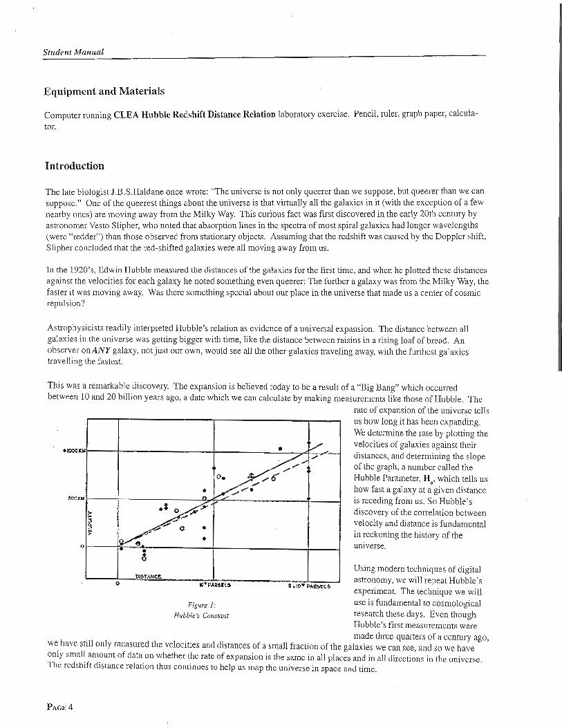
This was a remarkable discovery. The expansion is believed today to be a result of a "Big Bang" which occurred between 10 and 20 billion years ago, a date which we can calculate by making measurements like those of Hubble. The

rate of expansion of the universe tells us how long it has been expanding. We determine the rate by plotting the velocities of galaxies against their distances, and determining the slope of the graph, a number called the Hubble Parameter, Ho, which tells us how fast a galaxy at a given distance is receding from us. So Hubble's discovery of the correlation between velocity and distance is fundamental in reckoning the history of the universe.

Using modern techniques of digital astronomy, we will repeat Hubble's experiment. The technique we will

Figure 1: use is fundamental to cosmological ~ubble ' s Constant research these days. Even though

Hubble's first measurements were made three-quarters of a century ago,

we have still only measured the velocities and distances of a small fraction of the galaxies we can see, and so we have only small amount of data on whether the rate of expansion is the same in all places and in all directions in the universe. The redshift distance relation thus continues to help us map the universe in space and time.

Version 1.0

Technique

The software for the CLEA Hubble Redshift Distance Relation laboratory exercise puts you in control of a large optical telescope equipped with a TV camera and an electronic spectrometer. Using this equipment, you will determine the distance and velocity of several galaxies located in selected clusters around the sky. From these data you will plot a graph of velocity (the y-axis) versus distance (the x-axis).

How does the equipment work? The TV camera attached to the telescope allows you to see the galaxies, and "steer" the telescope so that light from a galaxy is focused into the slit of the spectro-meter. You can then turn on the spectrometer, which will begin to collect photons from the galaxy. The screen will show the spectrum-a plot of the intensity of light collected versus wavelength. When a sufficient number of photons are collected, you will be able to see distinct spectral lines from the galaxy (the H and K lines of calcium), and you will measure their wavelength using the computer cursor. The wavelengths will be longer than the wavelengths of the H and K labs measured from a non-moving object (397.0 and 393.3 nanometers), because the galaxy is moving away. The spectrometer also measures the apparent magnitude of the galaxy from the rate at which it receives photons from the galaxy. So for each galaxy you will have recorded the wave- lengths of the H and K lines and the apparent magnitude.

From the data collected above, you can calculate both the speed of the galaxy from the Doppler-shift formula, and the distance of the galaxy by comparing its known absolute magnitude (assumed to be (-22) for a typical galaxy) to its apparent magnitude. The result is a velocity (in kmlsec) and a distance (in megaparsecs, Mpc) for each galaxy. The galaxy clusters you will. observe have been chosen to be at different distances from the Milky Way, giving you a suitable range to see the straight line relationship Hubble first determined. The slope of the straight line will give you the value of Ha, the Hubble Parameter, which is a measure of the rate of expansion of the universe. Once you have Ha, you can take its reciprocal to find the age of the universe.

The details of the measurements and calculations are described in the following sections.

Using the Hubble Redshift Program

Welcome to the observatory! We will simulate an evening's observation during which we will collect data and draw conclusions on the rate of expansion of the universe. We will gain a proficiency in using the telescope to collect data by working together on the first object. Collecting data for the other four objects will be left to you to complete the evening's observing session. Then you will analyze the data, draw your conclusions, and use the information to predict the age of the universe.

Let's begin.

1. Open the Hubble Redshift program by double clicking on the Hubble Redshift Icon (pink). Click on Log in ... in the MENU BAR and enter student names and the lab table number. Click OK when ready.

2. The title screen of exercise appears. In the MXNU BAR, the only available (bold-faced) choices are to start or to quit, click on Start .

The Hubble Redshift Distance Relation program simulates the operation of a computer-controlled spectrometer attached to a telescope at a large mountain-top observatory. It is realistic in appearance, and is designed to give you a good feeling for how astronomers collect and analyze data for research.

The screen shows the control panel and view window as found in the "warm room" at the observatory. Notice that the dome is closed and tracking status is off.

Student Manual

3. To begin our evening's work, first open the dome by clicking on the dome button.

The dome opens and the view we see is from the finder scope. The finder scope is mounted on the side of the main telescope and points in the same direction. Because the field of view of the finder scope is much larger than the field of view of the main instrument, it is used to bx@ the objects we want to measure. The field of view is displayed on- screen by a CCD camera attached on the finder scope. (Note that it is not necessary for astronomers to view objects through an eyepiece.) Locate the Monitor button on the control panel and note its status, i.e. finder scope. Also note that the stars are drifting in the view window. This is due to the rotation of the earth and is very noticeable under high magnification of the finder telescope. It is even more noticeable in the main instrument which has even a higher magnification. In order to have the telescope keep an object centered over the spectrometer opening (slit) to collect data, we need to turn on the drive control motors on the telescope.

4. We do this by clicking on the tracking button.

The telescope will now track in sync with the stars. Before we can collect data we will need to do the following:

(a) Select a field of view (one is currently selected).

(b) Select an object to study (one from each field of view).

5 . To see the fields of study for tonight's observing session.

Click once on the change field item in the MENU BAR at the top of the control panel.

The items you see are the fields that contain the objects we have selected to study tonight. An astronomer would have selected these fields in advance of going to the telescope by:

(a) Selecting the objects that will be well placed for observing during the time we will be at the telescope.

(b) Looking up the RA and DEC of each object field in a catalog such as Uranometria 2000, Norton's Atlas, etc.

This list in the change field menu item contains 5 fields for study tonight. You will need to select one galaxy from each field of view and collect data with the spectrometer (a total of 5 galaxies).

To see how the telescope works, change the field of view to Ursa Major I1 at RA 11 hour 0 minutes and Dec. 56 degrees 48 min.

Notice the telescope "slews" (moves rapidly) to the RA and DEC coordinates we have selected. The view window will show a portion of the sky that was electronically captured by the charge coupled device (CCD) camera attached to the telescope.

The view window has two magnifications (see Figure 2 on next page):

Finder View is the view through the finder scope that gives a wide field of view and has a cross hair and outline of the instrument field of view.

Spectrometer View is the view from the main telescope with red lines that show the position of the slit of the spectrometer.

Version 1.0

Figure 2 Field of View from the Finder Scope

'JN.

)

".L3.. . ">.""'IY"

1% 5 9 i . . j 4 : i 2 e : l l n ~ t i o t . .

, . 41' Cl,"

Monitor .on F ~ n d e r . , .

u , 3 0 ' nn;. , , . Sel Cuurdinntes -

As in any image of the night sky, stars and galaxies are visible in the view window. It is easy to recognize bright galaxies in this lab simulation, since the shapes of the brighter galaxies are clearly different from the dot-like images of stars. But faint, distant galaxies can look similar to like stars, since we can't see their shape.

6. Now change fields by cliclung on Ursa Major I in the lists of selected galaxies to hghlight the field. Then click the OK button.

7 . Locate the Monitor button in the lower left hand portion of the screen. Click on this button to change the view from the Finder Scope to the Spectrometer. Using the Spectrometer view, carefully position the slit directly over the object you intend to use to collect data-any of the galaxies will be fine. Do this by "slewing", or moving, the telescope with the mouse and the N, S, E o r W buttons. Place the arrow on the N button and click on the left mouse button. To move continuously, press and hold down the left mouse button. Notice the red light comes on to indicate the telescope is "slewing" in that direction.

As in real observatories, it takes a bit of practice to move the telescope to an object. You can adjust the speed or "slew rate" of the telescope by using the mouse to press the slew rate button. (1 is the slowest and 16 is the fastest). When you have positioned the galaxy accurately over the slit, click on the take reading button to the right of the view screen.

The more light you get into your spectrometer, the stronger the.signal it will detect, and the shorter twill be the time required to get a usable spectrum. Try to position the spectrometer slit on the brightest portion of the galaxy. If you position it on the fainter parts of the galaxy, you are still able to obtain a good spectrum but the time required will be much longer. If you position the slit completely off the galaxy, you will just get a spectrum of the sky, which will be mostly random noise.

We are about to collect data from the object. We will be looking at the spectrum from the galaxy in the slit of the spectrometer. The spectrum of the galaxy will exhibit the characteristic H & K calcium lines which would normally appear at wavelengths 3968.847 and 3933.67 A, respectively, if the galaxies were not moving. However, the H & K lines will be red shifted to longer wavelengths depending on how fast the galaxy is receding.

Photons are collected one by one. We must collect a sufficient number of photons to allow identification of the wavelength. Since an incoming photon could be of any wavelength, we need to integrate for some time before we can accurately measure the spectrum and draw conclusions.

PAGE 7

Student Manual

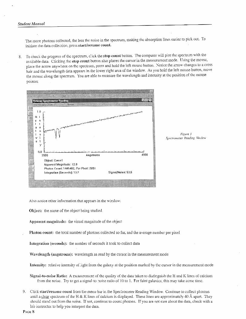
The more photons collected, the less the noise in the spectrum, making the absorption lines easier to pick out. To initiate the data collection, press startlresume count.

8. To check the progress of the spectrum, click the stop count button. The computer will plot the spectrum with the available data. Clicking the stop count button also places the cursor in the measurement mode. Using the mouse, place the arrow anywhere on the spectrum, press and hold the left mouse button. Notice the arrow changes to a cross hair and the wavelength data appears in the lower right area of the window. As you hold the left mouse button, move the mouse along the spectrum. You are able to measure the wavelength and intensity a.t the position of the mouse pointer.

te,i,mnm I. I - _- ' i d

Figure 3 Spectrotneter Reading Wndow

0.0 4 I 3 3900 Angstroms 4900 '

I

Apparent Magnitude: 12.8 Photon Count: 1445482, Per Pixel: 2891 Integration [Seconds]: 13.2 Signal/Noise: 53.5

Also notice other information that appears in the window:

Object: the name of the object being studied

Apparent magnitude: the visual magnitude of the object

Photon count: the total number of photons collected so far, and the average number per pixel

Integration (seconds): the number of seconds it took to collect data

Wavelength (angstroms): wavelength as read by the cursor in the measurement mode

Intensity: relative intensity of light from the galaxy at the position marked by the cursor in the measurement mode

Signal-to-noise Ratio: A measurement of the quality of the data taken to distinguish the H and K lines of calcium from the noise. Try to get a signal-to-noise ratio of 10 to 1. For faint galaxies, this may take some time.

9. Click startlresume count from the menu bar in the Spectrometer Reading Window. Continue to collect photons until a clear spectrum of the H & K lines of calcium is displayed. These lines are approximately 40 8, apart. They should. stand out from the noise. If not, continue to count photons. If you are not sure about the data, check with a lab instructor to help you interpret the data.

PAGE 8

Version 1.0

Additional information is needed to complete the analysis of the information that is not displayed in the spec- trometer reading window. They are the following: (a) The absolute magnitude (M) for all galaxies in this experiment. (b) The laboratory wavelength of the K line of calcium is 3933.67 a. (c) The laboratory wavelength of the H line of calcium is 3968.847 A.

10. Record the object, photon count, apparent magnitude, and the measured wavelength of the H & K lines of calcium on the data sheet located at the end of this exercise. The H & K lines measured should be red shifted from the labora- tory values depending on the galaxies motion.

11. To collect data for additional galaxies, press Return. Change the Monitor to display Finder, then follow steps 6 through 10.

Method

Now that we see how to use our instrument to collect data, we can use this information to determine for each galaxy, its distance and its velocity, using the following relationships:

l ~ o t e that we measure m and aisiirne a value for M in order to calculnre D (distance). Whcre D iq in parrecs.l

Ah, (B) V H = C * - and VK = C * - A x , A H A,

I Note that we measure1 (wivcreength) ln order to calculate v. I

1. Using the computer simulated telescope, measure and record on your data sheet the wavelengths of the calcium H and K lines for one galaxy in each of the fields selected for the evenings observation. Also, be sure to record the object name, apparent magnitude, and photon count. Round off numbers to two decimal places. Collect enough photons (usually around 40,000) to determine the wavelength of the line accurately.

2. Use your measured magnitudes and the assumed absolute magnitude for each galaxy and derive the distance, (D), to each galaxy using equation (A). Express your answer in both parsecs and megaparsecs in the appropriate places on your data table. Note that equation (A) tells you how to find the log of the distance.

Student Manual -

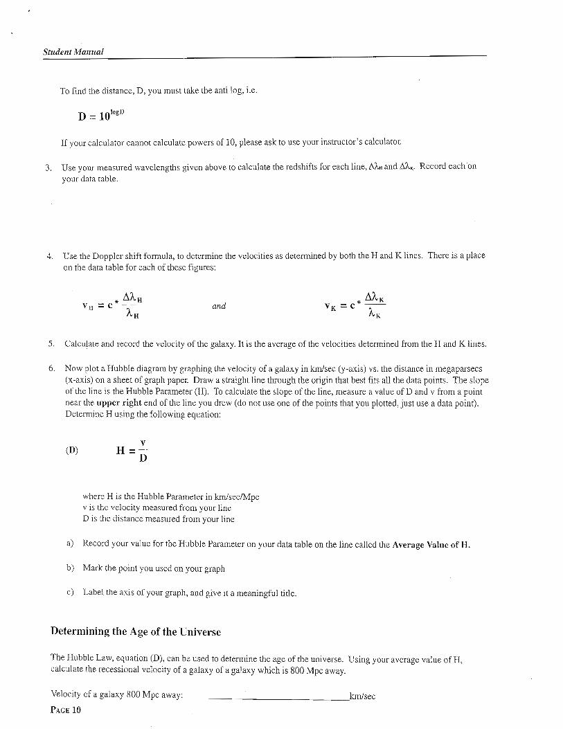
To find the distance, D, you must take the anti log, i.e,

D = 10 l0gD

If your calculator cannot calculate powers of 10, please ask to use your instructor's calculator.

3. Use your measured wavelengths given above to calculate the redshifts for each line, AhH and aK. Record each on your data table.

4. Use the Doppler shift formula, to determine the velocities as determined by both the H and K lines. There is a place on the data table for each of these figures:

and

5. Calculate and record the velocity of the galaxy. It is the average of the velocities determined from the H and K lines.

6. Now plot a Hubble diagram by graphing the velocity of a galaxy in kmlsec (y-axis) vs. the distance in megaparsecs (x-axis) on a sheet of graph paper. Draw a straight line through the origin that best fits all the data points. The slope of the line is the Hubble Parameter (H). To calculate the slope of the line, measure a value of D and v from a point near the upper right end of the line you drew (do not use one of the points that you plotted, just use a data point). Determine H using the following equation:

where H is the Hubble Parameter in km/sec/Mpc v is the velocity measured from your line D is the distance measured from your line

a) Record your value for the Hubble Parameter on your data table on the line called the Average Value of H.

b) Mark the point you used on your graph

c) Label the axis of your graph, and give it a meaningful title.

Determining the Age of the Universe

The Hubble Law, equation (D), can be used to determine the age of the universe. Using your average value of H, calculate the recessional velocity of a galaxy of a galaxy which is 800 Mpc away.

Velocity of a galaxy 800 Mpc away: - kmlsec

PAGE 10

Version 1.0

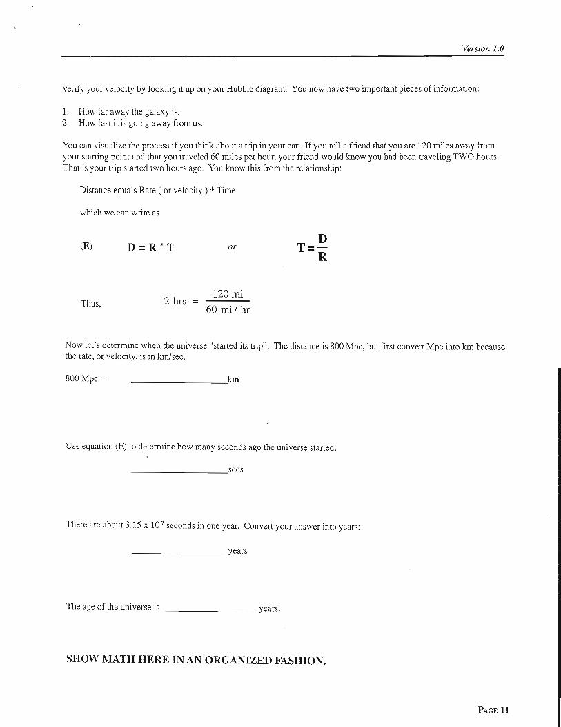
Verify your velocity by looking it up on your Hubble diagram. You now have two important pieces of information:

1. How far away the galaxy is. 2. How fast it is going away from us.

You can visualize the process if you think about a trip in your car. If you tell a friend that you are 120 miles away from your starting point and that you traveled 60 miles per hour, your friend would know you had been traveling TWO hours. That is your trip started two hours ago. You know this from the relationship:

Distance equals Rate ( or velocity ) * Time

which we can write as

Thus, 120 mi

2 hrs = 60 mil hr

Now let's determine when the universe "started its trip". The distance is SO0 Mpc, but first convert Mpc into km because the rate, or velocity, is in kmlsec.

800 Mpc = km

Use equation (E) to determine how many seconds ago the universe started:

There are about 3.15 x 10' seconds in one year. Convert your answer into years:

years

The age of the universe is years.

SHOW MATH HERE IN AN ORGANIZED FASHION.

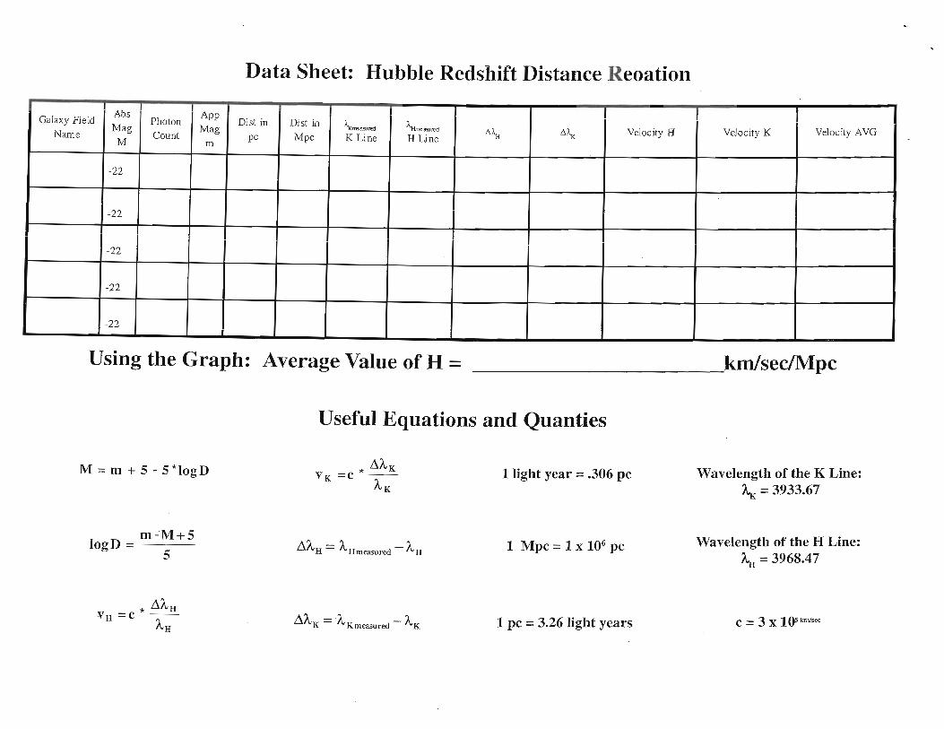
Data Sheet: Hubble Redshift Distance Reoation

Galaxy Field Abs

Photon Dii t in Distin A,,,,

Name Mag Count Mag pc *% *% Velocity H Velocity K Velocity AVG

M m Mpc K Line H Line

-22

-22

-22

-22 --- -22

Using the Graph: Average Value of H = km/sec/Mpc

Useful Equations and Quanties

1 light year = .306 pc

1 pc = 3.26 light years

Wavelength of the K Line: h, = 3933.67

Wavelength of the H Line: h, = 3968.47