Northumbria Research Link

Citation: Jackson, John (2004) Tight cosmological constraints from the angular-size/redshift relation for ultra-compact radio sources. Journal of Cosmology and Astroparticle Physics, 11. pp. 1-15. ISSN 1475-7508

Published by: IOP Publishing

URL: http://dx.doi.org/10.1088/1475-7516/2004/11/007 <http://dx.doi.org/10.1088/1475-7516/2004/11/007>

This version was downloaded from Northumbria Research Link: http://nrl.northumbria.ac.uk/1157/

Northumbria University has developed Northumbria Research Link (NRL) to enable users to access the University’s research output. Copyright © and moral rights for items on NRL are retained by the individual author(s) and/or other copyright owners. Single copies of full items can be reproduced, displayed or performed, and given to third parties in any format or medium for personal research or study, educational, or not-for-profit purposes without prior permission or charge, provided the authors, title and full bibliographic details are given, as well as a hyperlink and/or URL to the original metadata page. The content must not be changed in any way. Full items must not be sold commercially in any format or medium without formal permission of the copyright holder. The full policy is available online: http://nrl.northumbria.ac.uk/pol i cies.html

This document may differ from the final, published version of the research and has been made available online in accordance with publisher policies. To read and/or cite from the published version of the research, please visit the publisher’s website (a subscription may be required.)

Tight cosmological constraints from the

angular-size/redshift relation for ultra-compact

radio sources

J C Jackson†‡† Division of Mathematics and Statistics, School of Informatics, NorthumbriaUniversity, Ellison Place, Newcastle NE1 8ST, UK

Abstract.Some years ago (Jackson and Dodgson 1997) analysis of the angular-size/redshift

relationship for ultra-compact radio sources indicted that for spatially flat universes thebest choice of cosmological parameters was Ωm = 0.2 and ΩΛ = 0.8. Here I present anastrophysical model of these sources, based upon the idea that for those with redshiftz > 0.5 each measured angular size corresponds to a single compact component whichis moving relativistically towards the observer; this model gives a reasonable accountof their behaviour as standard measuring rods. A new analysis of the original data set(Gurvits 1994), taking into account possible selection effects which bias against largeobjects, gives Ωm = 0.24 + 0.09/− 0.07 for flat universes. The data points match thecorresponding theoretical curve very accurately out to z ∼ 3, and there is clear andsustained indication of the switch from acceleration to deceleration, which occurs atz = 0.85.

1. Introduction

The default cosmological paradigm now is that we are living in a spatially flat

accelerating Universe with matter (baryons plus Cold Dark Matter) and vacuum density-

parameters Ωm = 0.27 and ΩΛ = 0.73 respectively, known as the concordance model.

Definitive confirmation of a consensus which has been growing over the last two decades

came with the recent Wilkinson Microwave Anisotropy Probe (WMAP) results (Spergel

et al 2003). The original evidence for such models was circumstantial, in that they

reconcile the inflationary prediction of flatness with the observed low density of matter

(Peebles 1984; Turner et al 1984). The first real evidence came from observations

of very large-scale cosmological structures (Efstathiou et al 1990), which paper clearly

advocated everything that has come to be accepted in recent times: “......very large scale

cosmological structures can be accommodated in a spatially flat cosmology in which as

much as 80 percent of the critical density is provided by a positive cosmological constant.

In such a universe expansion was dominated by CDM until a recent epoch, but is now

governed by the cosmological constant.” A similar case for this model was made by

‡ To whom correspondence should be addressed (john.jackson@unn.ac.uk)

Tight cosmological constraints from the angular-size/redshift relation 2

Ostriker and Steinhardt (1995), who also noted that the location and magnitude of the

first Doppler peak in the cosmic microwave background (CMB) angular spectrum was

marginally supportive of flatness. However, the paradigm did not really begin to shift

until the Hubble diagram for Type Ia supernovae (SNe Ia) (Schmidt et al 1998; Riess et

al 1998; Perlmutter et al 1999) provided reasonably convincing evidence that ΩΛ > 0;

the corresponding confidence region in the Ωm–ΩΛ plane was large and elongated, but

almost entirely confined to the positive quadrant. The dramatic impact of these results

was probably occasioned by the simple nature of this classical cosmological test; coupled

with accurate measures of the first Doppler peak in the CMB angular spectrum (Balbi

et al 2000; de Bernardis et al 2000; Hanany et al 2000), which established flatness

to a high degree of accuracy, the SNe Ia results made anything but the concordance

model virtually untenable. This paper is in part retrospective, and is about another

simple classical cosmological test. Some years ago we published an analysis of the

angular-size/redshift diagram for milliarcsecond radio-sources (Jackson and Dodgson

1997; see also Jackson and Dodgson 1996), with a clear statement to the effect that “if

the Universe is spatially flat, then models with low density are favoured; the best such

model is Ωm = 0.2 and ΩΛ = 0.8”. This result pre-dates the SNe Ia ones.

Ultra-compact radio sources were first used in this context by Kellermann

(1993), who presented angular sizes for 79 objects, obtained using very-long-baseline

interferometry (VLBI). These were divided into 7 bins according to redshift z, and

the mean angular size θ plotted against the mean redshift for each bin. The main

effect of Kellermann’s work was to establish that the resulting θ–z relationship was

compatible with standard Friedmann-Lemaıtre-Robertson-Walker (FLRW) cosmological

models, in sharp contrast to the case for the extended radio structures associated with

radio-galaxies and quasars. In the latter case typical component separations are 30

arcseconds, and the observed relationship is the so-called Euclidean curve θ ∝ 1/z

(Legg 1970; Miley 1971; Kellermann 1972; Wardle and Miley 1974); this deficit of

large objects at high redshifts is believed to be an evolutionary effect, brought about

by interaction with an evolving extra-galactic medium (Miley 1971; Barthel and Miley

1988; Singal 1988), or a selection effect, due to an inverse correlation between linear

size and radio power (Jackson 1973; Richter 1973; Masson 1980; Nilsson et al 1993).

However, see Buchalter et al (1998) for a significant attempt to disentangle these effects.

Ultra-compact objects have short lifetimes and are much smaller than their parent active

galactic nuclei (AGNs), so that their local environment should be free of cosmological

evolutionary effects, at least over an appropriate redshift range. However, it is not clear

that observations of these objects are completely free from selection effects.

Kellermann’s work was extended by Gurvits (1994), who presented a large VLBI

compilation, based upon a 2.3 GHz survey undertaken by Preston et al (1985),

comprising 917 sources with a correlated flux limit of approximately 0.1 Jy; the sub-

sample selected by Gurvits comprises 337 sources with known redshifts, and objective

measures of angular size based upon fringe visibility (Thompson, Moran and Swenson

1986). Gurvits gave good reasons for ignoring sources with z < 0.5, and using just

Tight cosmological constraints from the angular-size/redshift relation 3

the high-redshift data found marginal support for a low-density FLRW model, but

considered only models with ΩΛ = 0. Jackson and Dodgson (1997) was based upon

Gurvits’ sample, and considered 256 sources in the redshift range 0.511 to 3.787, divided

into 16 bins of 16 objects. More recently Gurvits et al (1999) have presented a new

compilation of 330 compact radio sources, observed at a somewhat higher frequency

(ν = 5 GHz), which has stimulated a number of analyses (Vishwakarma 2001; Cunha

et al 2002; Lima and Alcaniz 2002; Zhu and Fujimoto 2002; Chen and Ratra 2003;

Jain et al 2003), which consider the full Ωm–ΩΛ plane and/or alternative models of the

vacuum. However, the constraints placed upon cosmological parameters by this later

work are significantly weaker than for example the SNe Ia constraints alone, and very

much weaker than those obtained when the latter are coupled with CMB and Large

Scale Structure observations (Efstathiou et al 1999; Bridle et al 1999; Lasenby, Bridle

and Hobson 2000; Efstathiou et al 2002).

The main purpose of this work is to show that angular-size/redshift data relating

to these sources place significant constraints upon cosmological parameters, comparable

with those due to any of the currently fashionable tests taken in isolation, and also

to establish a plausible astrophysical model which gives them credibility as putative

standard measuring rods. I find that the original Gurvits (1994) compilation better

in this respect than the later one due to Gurvits et al (1999), and I shall eventually

discuss why this might be so. The astrophysical model and associated selection effects

are discussed in Section 2, where evidence of such an effect is found. Appropriate

countermeasures are discussed in Section 3; these have some similarities to the scheme

adopted by Buchalter et al (1998) with regard to the extended radio sources, and the

parallels will be discussed. The corresponding cosmological results are presented as

marginalized confidence regions in the Ωm–ΩΛ plane, with some consideration of the

quintessence parameter w. It is in these considerations that this work is new, and differs

significantly from the analysis of essentially the same data in Jackson and Dodgson

(1997). At this stage I make no attempt to combine these data with other observations,

being content to show that the former deserve to be part of the cosmological cannon.

Quoted figures which depend upon Hubble’s constant correspond to H0 = 100 km sec−1

Mpc−1.

2. Selection effects and a source model

In a flux-limited sample sources observed at large redshifts are intrinsically the most

powerful, so that an inverse correlation between linear size and radio luminosity will

introduce a bias towards smaller objects. There are several reasons for expecting such

a correlation. On quite general grounds we would expect sources to be expanding,

and their luminosities to decrease with time after an initial rapid increase (Jackson

1973; Baldwin 1982; Blundell and Rawlings 1999). Additionally, Doppler beaming from

synchrotron components undergoing bulk relativistic motion towards the observer is

known to be important in compact sources, and Dabrowski et al (1995) have argued

Tight cosmological constraints from the angular-size/redshift relation 4

that this will introduce a similar correlation. Doppler boosting was first discussed by

Shklovsky (1964a,b), to explain the apparently one-sided jet in M87. Subsequently Rees

(1966) devised a relativistically expanding model with spherical symmetry, to account

for the rapid variability observed in powerful radio sources, and noted that apparently

superluminal motion should be seen in such models, some ten years before this phenomen

was observed (Cohen 1975; Cohen et al 1976, 1977). Shklovsky’s basic twin-jet model

has been the subject of many elaborations over the past three decades, and Doppler

boosting is now the basis of the so called unified model of compact radio sources, in which

orientation effects in an essentially homogeneous population generate the full range of

observed properties. The notion that quasi-stellar radio sources are just a small subset

of apparently radio-quiet quasi-stellar objects (QSOs), that is those which are viewed

in the appropriate orientation, was first discussed by Scheuer and Readhead (1979),

and subsequently by Orr and Browne (1982), who concluded that some QSOs must be

genuinely radio quiet. Particulary germane to the discussion below are Blandford and

Konigl (1979a), Blandford and Konigl (1979b) and Lind and Blandford (1985). This is

not intended to be a comprehensive historical review, examples of which can be found

in Blandford et al (1977) and Kellerman (1994).

The underlying source population probably consists of compact symmetric objects

(CSOs), of the sort observed by Wilkinson et al (1994) at moderate redshifts

(0.2 <∼ z <

∼ 0.5), with radio luminosity densities of several times 1026 W Hz−1 at 5

GHz; these comprise central low-luminosity cores straddled by two mini-lobes, the

former contributing no more than a few percent of the total luminosity (Readhead

et al 1996a); without Doppler boosting these objects would be too faint to be observed

at higher redshifts. It is thus reasonable to suppose that in the most distantly observed

cases the lobes are moving relativistically and are close to the line of sight. For this

reason the use of ultra-compact sources as standard measuring rods has been questioned

by Dabrowski et al (1995), who consider a simple model, comprising two identical but

oppositely directed jets (treated as point or line sources), and assume that the measured

angular size corresponds to their separation projected onto the plane of the sky; thus

apparent radio power increases and angular size decreases as the beams get closer to the

line of sight. However, this model is not realistic, as the counter-jet would be very much

fainter than the forward one, for example by a factor of up to 106 for a jet Lorentz factor

γ of 5. It is more reasonable to suppose that we observe just that component which is

moving relativistically towards the observer, and in particular that the interferometric

angular sizes upon which this work is based correspond to the said components.

It is reasonable to ask if the above supposition is compatible with VLBI images

of distant AGNs and quasars. At first sight this is not the case; it is well-known that

these images typically show a core/one-sided jet structure (see for example Taylor et

al 1996), rather than a single component. However, it is well-known that there is

an inconsistency here, if the cores are to be identified with those of the underlying

CSO population and the latter are unbeamed. The problem then is that as mentioned

above members of the CSO population are typically jet dominated, and would become

Tight cosmological constraints from the angular-size/redshift relation 5

distinctly more so when viewed close to the jet axis, by several orders of magnitude,

which is not what is observed; in VLBI images of distant sources the core is usually

dominant, and the jet is often absent. This dilema has been resolved by Blandford

and Konigl (1979a,b), who describe a model in which the ‘core’ is really part of the

jet, and is thus also Doppler boosted (see also Kellerman 1994). In their model the

core emmission originates in the stationary compact end of a quasi-steady supersonic

jet, where the latter becomes optically thick; the so called jet emmission comes from

up-stream shock waves associated with dense condensations within the bulk flow which

are being accelerated by the latter. A stationary core which is nevertheless relativistic is

necessary, to reconcile superluminal expansion with the observed relative fluxes from the

two components. In the latter respect it is essential that γj < γc (where subscripts c and

j denote core and jet respectively), but this is part of the Blandford and Konigl (1979a,b)

model; jet domination then changes into core domination as φ changes from π/2 to zero,

where φ be the angle between the jet axis and the line-of-sight; the transverse Doppler

effect diminishes the core relative to the jet when φ = π/2, but the roles are reversed

when φ = 0. In other words the core emission is more beamed than that of the jet.

If the two components have flat spectra and the same rest-frame luminosities, and

R(φ) is the core/jet luminosity ratio, then

R(0) =

(γcγj

)n

and R(π/2) =

(γjγc

)n

(1)

and the crossover angle at which R = 1 is φ ∼ (γjγc)−1/2 (see below for the definition of

n). A ratio γc/γj ∼ 2 to 3 would effect a transition of the correct magnitude; for typical

values of γ the crossover angle is 15 to 20.If the basic model outlined above is correct, one consequence is that statistically

cores are observed at something like a fixed rest-frame frequency; suppose that a core

has rest-frame luminosity density L, with flat spectral index α = 0 characteristic of

ultra-compact sources. The Doppler boosting factor D is

D = γ−1(1− β cos φ)−1 (2)

where β is the object velocity in units of c, and as above φ is the angle between this

velocity and the line of sight. For a source at redshift z and angular-diameter distance

DA(z), the observed flux density S is thus

S =LDn

4π(1 + z)3D2A

⇒ D1 + z

=

(4πD2

AS

L

)1/n

(1 + z)(3−n)/n (3)

where n = 3 for discrete ejecta and n = 2 for a continuous jet (Lind and Blandford

1985). As we have seen, in reality the situation lies between these two extremes, and a

value n = 5/2 will be used for purposes of illustration. In the redshift range of interest

DA(z) is close to its minimum, and is thus a slowly varying function of z, so that for an

object observed close to the flux-limit the ratio D/(1 + z) is proportional to (1 + z)1/5

Tight cosmological constraints from the angular-size/redshift relation 6

and is roughly fixed † : the survey frequency of 2.3 GHz corresponds to a rest-frame

frequency of 2.3 GHz divided by this ratio, which would for example greatly reduce

the effect, deleterious in this context, of any dependence of linear size on rest-frame

frequency. Similar considerations apply to jets if γj/γc is fixed.

It has been noted by Frey and Gurvits (1997) that jets become noticeably less

prominent, in terms of both morphology and luminosity, as redshift increases. At z > 3

jets appear to be absent or vestigial (see for example the VLBI images presented by

Gurvits et al 1994, Frey et al 1997 and Paragi et al 1999). Frey and Gurvits (1997)

reasonably attribute this phenomenon to differential spectral properties, cores being

flatter than the jets in this respect. However, if statistically the cosmological redshift

is roughly cancelled out by the Doppler boost, as suggested in the last paragraph,

then spectral differences should be not be as important as Frey and Gurvits (1997)

suppose. In part the phenomenon is probably the Dabrowski et al (1995) selection

effect in operation: the viewing angle φ gets smaller as z increases, and projecion effects

mean that the two components first overlap and then become superimposed, when we

see a single composite source. Such selection is thus not as significant as Dabrowski et

al (1995) suggest, particularly at high redshifts, because the components are not point

sources, and angular sizes do not vanish as the beams get closer to the line of sight.

At lower redshifts we see more structure; cursory inspection of 113 VLBI images (not

redshift selected) presented by Taylor et al (1996) suggests that about one third of these

are superimposed composites, one third are core/jet overlaps, and one third show two

separate components or more complex structures. However, Dabrowski et al (1995) show

that their effect is not significant at low redshifts, typically z <∼ 1.5 for the flux limit of

0.1 Jy which characterises this sample. Thus over the full redshift range it is reasonable

to suppose that this particular selection is of marginal importance. The matter will

be discussed further, when suitable countermeasures are considered. Although these

considerations are interesting from an astrophysical point of view, their significance

here is to identify these superimposed core/jet composites as the components which in

effect determine the measured angular sizes upon which this work is based.

Finally, with regard to establishing ultra-compact sources as standard linear

measures, I note that the parent galaxies in which they are embedded are giant ellipticals,

with masses close 1013M¯; it is known that their central black holes have masses which

are tightly correlated with this mass (Kormendy 2001a,b), being 0.15% of same, close

to 1.5 × 1010M¯. The central engines which power these sources are thus reasonably

standard objects.

The question of whether there is a linear-size/luminosity correlation of the sort

discussed at the beginning of this section is easily settled; Figure 1 is a plot of linear

extent d (as indicated by the measured angular size) against correlated rest-frame

luminosity L (attributable to the compact component, and calculated assuming isotropic

emission and a spectral index α = −0.1, where L ∝ ν−α), for a selection of redshift bins,

† This approximation gets better if the slow changes in DA(z) are taken into account.

Tight cosmological constraints from the angular-size/redshift relation 7

each containing 16 sources from the Gurvits (1994) sample. A cosmology is needed for

this plot, and I have pre-empted the results to be presented here by using Ωm = 0.24

and ΩΛ = 0.76; however, the significant qualitative aspects of the arguments I shall

present are not sensitive to this choice. There is clear evidence that at any particular

epoch individual luminosities are a function of size, and that for sources with z >∼ 0.2 this

relationship is an inverse correlation. For z > 0.5 the relationship is well-represented by

L ∝ d−a (4)

where in round figures a = 3. In the above model, this behaviour would be attributed

to expansion of each relativistic component as it moves away from the central engine

and grows weaker. However, as noted by Gurvits (1994), the remarkable feature of this

diagram is that for z > 0.5 there is no marked change in mean size at a given luminosity,

over a range of the latter variable which covers three orders of magnitude, which suggests

that these two parameters are decoupled. This behaviour is quite compatible with the

model outlined above; a tentative subdivision is that for z < 0.2 these sources are

intrinsically small and weak and not relativistic; between z = 0.2 and z = 0.5 there is a

transitional regime, during which the intrinsic luminosity rises to several times 1026 W

Hz−1; thereafter the latter is approximately fixed, the sources are ultra-relativistic, and

the luminosity range is accounted for largely by changes in Doppler boost. For example

with fixed γ = 5, a luminosity boost factor D2.5 varies by a factor of 316 as φ changes

from 0 to 35. A similar phenomenon has been noted in X-ray astronomy (Fabian et

al 1997).

The sub-division outlined above is analogous to the division of extended double

radio sources into Fanaroff-Riley types I and II (FR-I and FR-II) (Fanaroff and Riley

1974; Kembhavi and Narlikar 1999). The radio morphologies of FR-I sources typically

show a relatively bright central core from which bright opposed jets emanate in

symmetric fashion, which jets terminate in faint diffuse lobes as they run into the inter-

galactic medium. FR-II sources typically comprise a relatively faint core with a one-sided

jet which terminates in a bright compact lobe, with a comparable lobe on the opposite

side of the core, but no sign of a corresponding counter-jet; presumably the latter is

invisible due to beaming. FR-I sources are relatively weak, having radio luminosities

L(2.3 GHz) <∼ 2 × 1024 W Hz−1, whereas FR-II sources are intrinsically strong, having

luminosities greater than this figure. Although this threshold luminosity is two orders of

magnitude lower than the luminosities associated with the CSOs observed by Wilkinson

et al (1994), it may be that the analogy is exact, in that the latter are the precursors of

FR-I objects, if luminosity evolution is invoked (Readhead et al 1996b). Similarly, the

more distant compact objects discussed here may be the precursors of FR-II sources.

Buchalter et al (1998) select FR-II sources as the basis of their work on the angular-

size/redshift relation, in part because their morphology allows an objective definition

angular size. This selection was effected by choosing sufficiently powerful sources having

z > 0.3 and the correct radio morpology. Buchalter et al (1998) must then first

allow for a lower size cut-off, below which the FR-I/FR-II classification is beyond the

Tight cosmological constraints from the angular-size/redshift relation 8

resolving power of the instruments in question. Finally Buchalter et al (1998) allow for

a linear-size/redshift correlation of the sort discussed above, by assuming d ∝ (1 + z)c

and allowing the data to fix the constant c, which represents a combination of several

effects. Such measures appear to be necessary, if the angular-size/redshift diagram for

extended sources is to be in concordance with acceptible FLRW cosmological models,

but the situation is then too degenerate to make definitive statements about cosmological

parameters. As we shall see in the next section, milliarcseconds sources are more robust

in this respect, and although similar measures will be introduced, they are a refinement

rather than a necessity.

Because we cannot measure absolute visual magnitudes or linear sizes directly, it is

essential to have a model which supports the choice of the objects in question as standard

candles or standard measuring rods. In the case of Type Ia supernovae such support is

provided by a reasonably well-established model, based upon accreting Chandrasekhar-

mass white dwarfs in binary systems (Branch et al 1995; Livio 2001). I believe that the

above model provides similar support for powerful ultra-compact radio sources and the

angular-size/redshift diagram.

3. Cosmological parameters

As in Gurvits (1994) and Jackson and Dogson (1997), I shall consider only those sources

with z > 0.5, amply justified by the discussion above. It is clear that as individual

objects these do not have fixed linear dimensions, and we must consider the population

mean. Accordingly, the sources are placed in redshift bins, and earlier practice would be

to plot simple means for each bin in a θ–z diagram. However, due to the selection biases

discussed in Section 2, a growing proportion of the larger members of this population will

be lost as redshift increases, and simple means introduce a systematic error. According

to the adopted model, the effect can be quantified. The flux limit Sc sets a cut-off size

dc at each redshift, such that sources larger than dc are too faint to be observed. Again

taking a flat spectrum, equations (3) and (4) with a = 3 give

dc ∝ Dn/3

(4πD2ASc)1/3(1 + z)

. (5)

Thus assuming that there is a largest boost factor D which does not change with redshift,

and noting that in the redshift range of interest DA(z) is close to its minimum, we find

dc ∝ (1 + z)−1. (6)

Figure 2 is a plot of linear extent against z for all 337 sources in the Gurvits (1994)

sample. The dashed line shows dc(z) according to equation (6), normalized to give

dc = 20 pc at z = 1. Figure 2 appears to show that the larger objects are being lost

when z exceeds 1.5, in a manner which is in reasonable accord with equation (6). I have

adopted the following pragmatic procedure to reduce the concomitant systematic error;

instead of simple means I have defined a lower envelope for the data. An obvious choice

Tight cosmological constraints from the angular-size/redshift relation 9

would be the lowest point within each bin, but this is too noisy. I have defined the

lower envelope as the boundary between the bottom third and the top two thirds of the

points within each bin, in other words a median which gives more weight to the smaller

objects. Note however that this prescription is not tied to the particular model of bias

discussed in Section 2; it is an empirical measure based upon the observation that larger

sources appear to be weaker, and its effect would be neutral otherwise. (Gurvtis et al

(1999) use ordinary median angular sizes rather than means, to reduce the influence

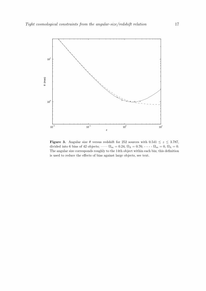
of outliers, which is an added benefit here.) Figure 3 shows 6 weighted median points;

each of these derives from a bin containing 42 objects, being the mean of points 11 to

17 within each bin, counting from the smallest object; the sample thus comprises 252

objects in the range 0.541 ≤ z ≤ 3.787. Error bars are ± one standard deviation as

determined by the said points; they are shown as an indication of the efficacy of this

definition of lower boundary, and are not used in the statistical analysis which follows.

I have experimented with various bin sizes; the reasons for this particular choice will be

discussed later. In all cases means are means of the logarithms.

A simple three-parameter least-squares fit to the points in Figure 3 gives optimum

values Ωm = 0.29, ΩΛ = 0.37 and median size d = 5.7 parsecs. If the model is constrained

to be flat, then a two-parameter least-squares fit gives optimum values Ωm = 0.24,

ΩΛ = 1−Ωm = 0.76 and d = 6.2 parsecs, which model is shown as the continuous curve

in Figure 3; the latter also shows the zero-acceleration model Ωm = 0, ΩΛ = 0, d = 6.2

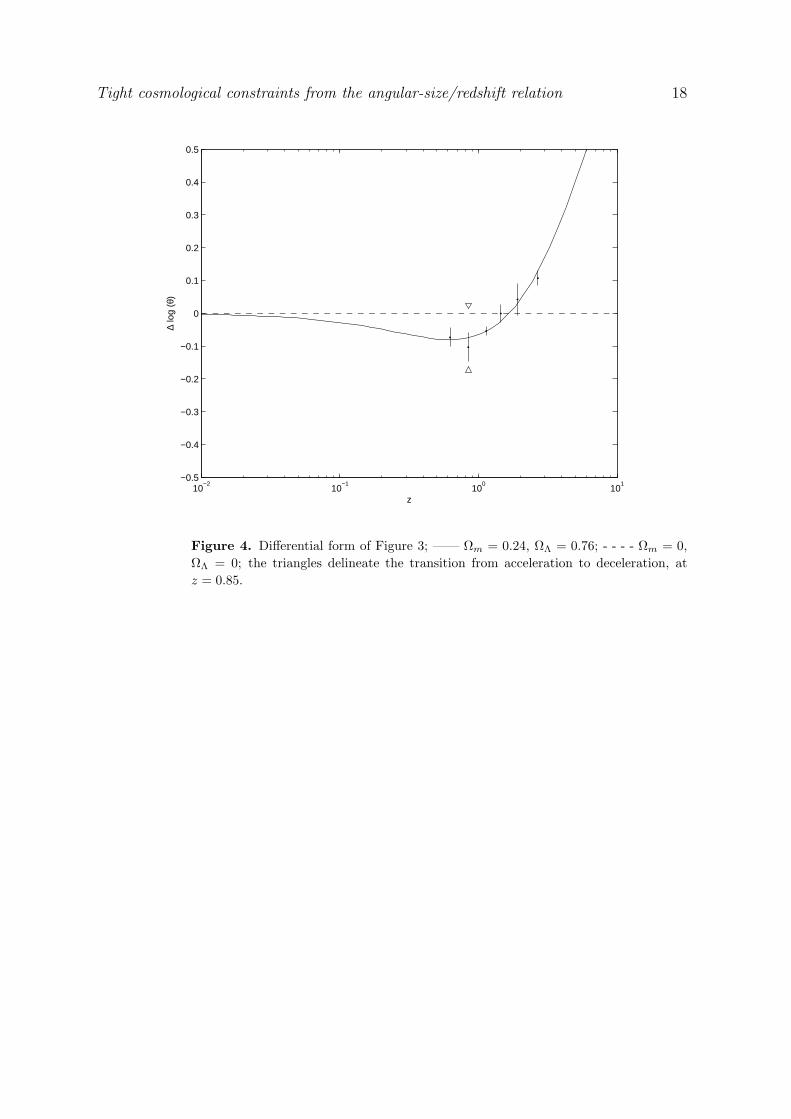
pc as the dashed curve. The difference ∆ log(θ) between the two curves is presented in

Figure 4, which shows clearly the shift from acceleration to deceleration. Note however

that the actual switch occurs before the crossing point, at z = (2ΩΛ/Ωm)1/3−1 = 0.85 in

this case, roughly where the continuous curve begins to swing back towards the dashed

one. Figure 4 establishes definitively and accurately that there is no need to invoke

anything other than a simple Ωm–ΩΛ model to account for the data, out to a redshift

z = 2.69. The current record for SNe Ia is SN 1997ff at z ∼ 1.7 (Gilliand and Phillips

1998; Riess et al 2001), with a somewhat uncertain apparent magnitude.

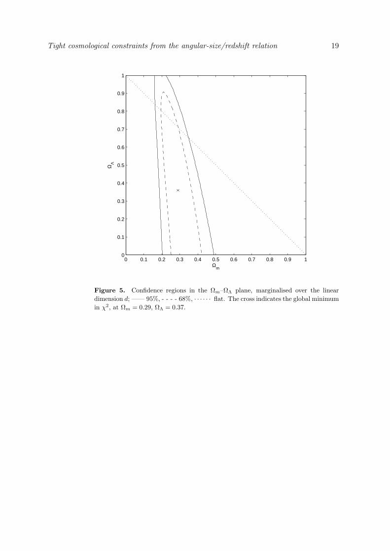
In order to derive confidence regions, I have defined a fixed standard deviation σ

to be attached to each point in Figure 3: σ2 = residual sum-of-squares/(n − p), where

n = 6 is the number of points and p = 3 is the number of fitted parameters, giving

σ = 0.0099 in log θ in this case. This value of σ is used to calculate χ2 values at

points in a suitable region of parameter space. Figure 5 shows confidence regions in

the Ωm–ΩΛ plane derived in this manner, marginalized over d according to the scheme

outlined in Press et al (1986). Without the extra constraint of flatness little can be said

about ΩΛ, which degeneracy is due to the lack of data points with z < 0.5 (Jackson

and Dodgson 1996). Nevertheless Figure 5 clearly constrains Ωm to be significantly less

than unity. Figure 5 is essentially a refined and tighter version of the diagram presented

in Jackson and Dodgson (1997); the significant change is that flat models are now well

within the 68% confidence region, whereas previously the figure was 95%; this change

is entirely due to the measures relating to selection effects. In the case of flat models,

two-dimensional confidence regions can be presented without marginalization. Figure 6

Tight cosmological constraints from the angular-size/redshift relation 10

shows such regions in the Ωm–d plane; marginalizing over d gives 95% confidence limits

Ωm = 0.24 + 0.09/− 0.07.

With respect to choice of redshift binning the balance is between many bins

containing few objects and a small number containing many objects; the former gives

poor estimates of population parameters within each bin, but a large number of points

to work with in Figure 3; the latter gives better estimates of these parameters but

fewer points in Figure 3. I have experimented with 15 bin sizes, from 17 bins of 15

objects to 4 bins of 57 objects, in steps of 3 objects; in each case I have used the largest

number of bins compatible with having no objects with z ≤ 0.5. I find that the central

figure is quite robust, but that accuracy increases gradually as the number of bins is

reduced, the best compromise being the one used above. As a check I have calculated

the best cosmological parameters in each of the 15 cases, and when selection effects are

allowed for I find a mean value Ωm = 0.25 in the flat case, with 95% confidence limits

of ±0.06. If selection effects are ignored corresponding figures are virtually the same,

Ωm = 0.24±0.04, again in the flat case. However, this coincidence understates the value

of the measures relating to selection bias; as mentioned above, these bring flat models

well within the 68% confidence region in Figure 5, and more importantly they reveal

the expected minimum angular size in Figure 3 (Hoyle 1959).

As already noted with respect to Figure 4, simple Ωm–ΩΛ models give an excellent

fit to the data. Nevertheless, in conclusion I consider the limits placed upon the

quintessence parameter w, defined by postulating an equation of state for the vacuum

of the form ρvac = wpvac relating the vacuum density ρvac to the vacuum pressure pvac,

with |w| ≤ 1 and w = −1 corresponding to the conventional vacuum defined by a

cosmological constant. For flat models we have a three-parameter system comprising

Ωm, w and d, the quintessence parameter Ωq being 1−Ωm; we proceed by marginalising

over d to give the two-parameter confidence regions shown in Figure 7. The system

is highly degenerate, and with respect to material content cannot distinguish between

between for example a two component mix with Ωm = 0.24, Ωq = 0.76, w = −1 at one

extreme, and a single component compromise with Ωm = 0, Ωq = 1, w = −0.37 at the

other. Lacking any compelling evidence to the contrary, the sensible choice is to retain

local Lorentz invariance and assume that w = −1.

4. Conclusions

The prescription adumbrated here has produced a set of data points which are

remarkably consistent with Ωm–ΩΛ FLRW cosmological models, but there is extensive

degeneracy due to the restricted redshift range. This degeneracy is resolved by

combining angular-size/redshift data with that CMBR information which indicates

flatness, and the two data sets together give Ωm = 0.24 + 0.09/− 0.07. This compares

well with the figure Ωm = 0.27±0.04 arising from WMAP measurements combined with

a host of other astronomical data sets (Spergel et al 2003); the points generated in this

work might be added as an extra data set; for future reference these are given in Table

Tight cosmological constraints from the angular-size/redshift relation 11

1.

Table 1. Data points for the angular-size/redshift relationship; θ is in milliarcseconds.

z θ

0.623 1.2770.845 1.0891.138 1.0341.450 1.0231.912 1.0082.686 1.024

This work builds upon the earlier work of Jackson and Dodgson (1997), and shows

that the results obtained there were not spurious. Its purpose goes beyond that of

showing compatibility with more recent work, and suggests that building a much larger

angular-size/redshift data set for ultra-compact sources would be a promising enterprise.

VLBI resolution of a quasar at z = 5.82 has been demonstrated (Frey et al 2003), so

that the redshift limit of such a data set should go well beyond that expected of the

Supernova/Accleration probe (SNAP) (Aldering et al 2004), approaching 6 rather than

1.7. Additionally, this approach is immune to effects which might invalidate the SNe Ia

results, such as absorption by grey dust, as has been noted by others (Bassett and Kunz

2004a; Bassett and Kunz 2004b). The two approaches are of course complementary in

their redshift ranges, rather than competitive. Section 2 might act as a guide to further

work, particularly with regard to reducing the effects of selection. Additionally, samples

might be filtered using morphological considerations, to include only those objects which

show roughly circular symmetry, corresponding to the superimposed core/jet composites

discussed in Section 2, which procedure would be similar to that adopted by Buchalter et

al (1998) in their selection of FR-II sources. A related proposal due to Wiik and Valtaoja

(2001) is that the linear sizes of shocks within jets might be estimated directly for each

object, using flux density variations and light travel time arguments, so that each object

would become a separate point in the angular-size/redshift diagram; a weakness in their

case is that individual Doppler boosts have to be estimated.

I must end on a cautionary note; in general results from the 5GHz sample due

to Gurvits et al (1999) are compatible with the ones presented here, but with much

greater uncertainty (Chen and Batra 2003); the prescription developed here does not

significantly improve matters in this respect. The probable reason for this difference in

behaviour is the definition of angular size; in Gurvits et al (1999) this is defined as the

distance between the strongest component and the most distant one with peak brightness

≥ 2% of that of the strongest component; here the objective measure based upon fringe

visibility ignores such outliers and estimates the size of the dominant component.

Tight cosmological constraints from the angular-size/redshift relation 12

References

Aldering G et al 2004 Preprint astro-ph/0405232Balbi A, Ade P, Bock J, Borrill J, Boscaleri A, De Bernardis P, Ferreira P G, Hanany S, Hristov V,

Jaffe A H, Lee A T, Oh S, Pascale E, Rabii B, Richards P L, Smoot G F, Stompor R, Winant CD and Wu J H P 2000 Astrophys. J. 545 L1

Baldwin J E 1982 Proc. IAU Symp. 97 (Dordrecht: Reidel) p 21Barthel P D and Miley G K 1988 Nature 333 319Bassett B A and Kunz M 2004a Astrophys. J. 607 661Bassett B A and Kunz M 2004b Phys. Rev. D 69 101305Blandford R D, McKee C F and Rees M J 1977 Nature 267 211Blandford R D and Konigl A 1979a Astrophys. Lett. 20 15Blandford R D and Konigl A 1979b Astrophys. J. 232 34Blundell K M and Rawlings S 1999 Nature 399 330Branch D, Livio M, Yungelson L R, Boffi F R, Baron E and Baron E 1995 Proc. Astron. Soc. Pacific

107 1019Bridle S L, Eke, V R, Lahav O, Lasenby A N, Hobson M P, Cole S, Frenk C S and Henry J P 1999

Mon. Not. R. Astron. Soc. 310 565Buchalter A, Helfand D J, Becker R H and White R L 1998 Astrophys. J. 494 503Chen G and Ratra B 2003 Astrophys. J. 582 586Cohen M H 1975 Ann. N. Y. Acad. Sci. 262 428Cohen M H, Moffet A T, Romney J D, Schilizzi R T, Seielstad G A, Kellermann K I, Purcell G H,

Shaffer D B, Pauliny-Toth I I K and Preuss E 1976 Astrophys. J. 206 L1Cohen M H, Linfield R P, Moffet A T, Seielstad G A, Kellermann K I, Shaffer D B, Pauliny-Toth I I

K, Preuss E, Witzel A and Romney J D 1977 Nature 268 405Cunha J V, Alcaniz J S and Lima J A 2002 Phys. Rev. D 66 023520Dabrowski Y, Lasenby A and Saunders R 1995 Mon. Not. R. Astron. Soc. 277 753de Bernardis P et al 2000 Nature 404 955Efstathiou G, Sutherland W J and Maddox S J 1990 Nature 348 705Efstathiou G, Bridle S L, Lasenby A N, Hobson M P and Ellis R S 1999 Mon. Not. R. Astron. Soc.

303 L47Efstathiou G et al 2002 Mon. Not. R. Astron. Soc. 330 L29Fabian A C, Brandt W N, McMahon R G and Hook I M 1997 Mon. Not. R. Astron. Soc. 291 L5Fanaroff B L and Riley J M 1974 Mon. Not. R. Astron. Soc. 167 31PFrey S and Gurvits L I, 1997 Vistas Astron. 41 271Frey S, Gurvits L I, Kellermann K I, Schilizzi R T and Pauliny-Toth I I K 1997 Astron. Astrophys.

325 511Frey S, Mosoni L, Paragi Z and Gurvits L I 2003 Mon. Not. R. Astron. Soc. 343 L20Gilliland R L and Phillips M M 1998 IAU Circ. 6810Gurvits L I 1994 Astrophys. J. 425 442Gurvits L I, Schilizzi R T, Barthel P D, Kardashev N S, Kellermann K I, Lobanov A P, Pauliny-Toth

I I K and Popov M V 1994 Astron. Astrophys. 291 737Gurvits L I, Kellermann K I and Frey S 1999 Astron. Astrophys. 342 378Hanany S et al 2000 Astrophys. J. 545 L5Hoyle F 1959 Proc. IAU Symp. 9: Paris Symposium on Radio Astronomy (Stanford: Stanford

University Press) p 529Jackson J C 1973 Mon. Not. R. Astron. Soc. 162 11PJackson J C and Dodgson M 1996 Mon. Not. R. Astron. Soc. 278, 603Jackson J C and Dodgson M 1997 Mon. Not. R. Astron. Soc. 285, 806Jain D, Dev A and Alcaniz J S 2003 Class. Quant. Grav. 20 4485

Tight cosmological constraints from the angular-size/redshift relation 13

Kembhavi A K and Narlikar J V 1999 Quasars and Active Galactic Nuclei (Cambridge: CambridgeUniversity Press) chapter 9

Kellermann K I 1972 Astronom. J. 77 531Kellermann K I 1993 Nature 361 134Kellermann K I 1994 Aust. J. Phys. 47 599Kormendy J 2001a ASP Conf. Ser. 230: Galaxy Disks and Disk Galaxies (San Francisco: Astronomical

Society of the Pacific) p 247Kormendy J 2001b Rev. Mex. Astronom. Astrofs. (Serie de Conferencias) 10 69Lasenby A N, Bridle S L and Hobson M P 2000 Astrophys. Lett. & Communications 37 327Legg T H 1970 Nature 226 65Lind K R and Blandford R D 1985 Astrophys. J. 295 358Livio M 2001 Proc. STScI Symp. 13: Supernovae and Gamma-Ray Bursts (Cambridge: Cambridge

Univ. Press) p 334Lima J A S and Alcaniz J S 2002 Astrophys. J. 566 15Masson C R 1980 Astrophys. J. 242 8Miley G K, 1971 Mon. Not. R. Astron. Soc. 152 477Nilsson K, Valtonen M J, Kotilainen J and Jaakkola T 1993 Astrophys. J. 413 453Orr M J L and Browne I W A 1982 Mon. Not. R. Astron. Soc. 200 1067Ostriker J P and Steinhardt P J 1995 Nature 377 600Paragi Z, Frey S, Gurvits L I, Kellermann K I, Schilizzi R T, McMahon R G, Hook I M and Pauliny-Toth

I I K 1999 Astron. Astrophys. 344 51Peebles P J E 1984 Astrophys. J. 284 439Perlmutter S et al 1999 Astrophys. J. 517 565Press W H, Flannery B P, Teukolsky S A and Vetterling W T 1986 Numerical Recipes (Cambridge:

Cambridge University Press) pp 532–536Preston R A, Morabito D D, Williams J G, Faulkner J, Jauncey D L, Nicolson G 1985 Astronom. J.

90 1599Readhead A C S, Taylor G B, Xu W, Pearson T J, Wilkinson P N, Polatidis A G 1996a Astrophys. J.

460 612Readhead A C S, Taylor G B, Pearson T J, Wilkinson P N 1996b Astrophys. J. 460 634Rees M 1966 Nature 211 468Richter G M 1973 Astrophys. Lett. 13 63Riess A G, Filippenko A V, Challis P, Clocchiatti A, Diercks A, Garnavich P M, Gilliland R L, Hogan

C J, Jha S, Kirshner R P, Leibundgut B, Phillips M M, Reiss D, Schmidt B P, Schommer R A,Smith R C, Spyromilio J, Stubbs C, Suntzeff N B and Tonry J 1998 Astronom. J. 116 1009

Riess A G, Nugent P E, Gilliland R L, Schmidt B P, Tonry J, Dickinson M, Thompson R I, Budavri T,Casertano S, Evans A S, Filippenko A V, Livio M, Sanders D B, Shapley A E, Spinrad H, SteidelC C, Stern D, Surace J and Veilleux S 2001 Astrophys. J. 560 49

Scheuer P G A and Readhead A C S 1979 Nature 277 182Schmidt B P et al 1998 Astrophys. J. 507 46Shklovsky I S 1964a Soviet Astron.–AJ 7 748Shklovsky I S 1964b Soviet Astron.–AJ 7 972Singal A K 1988 Mon. Not. R. Astron. Soc. 233 87Spergel D N, Verde L, Peiris H V, Komatsu E, Nolta M R, Bennett C L, Halpern M, Hinshaw G,

Jarosik N, Kogut A, Limon M, Meyer S S, Page L, Tucker G S, Weiland J L, Wollack E and WrightE L 2003 Astrophys. J. Suppl. 148 175

Taylor G B, Vermeulen R C, Readhead A C S, Pearson T J, Henstock D R, and Wilkinson P N 1996Astrophys. J. Suppl. 107 37

Thompson A R, Moran J M and Swenson G W Jr 1986 Interferometry and Synthesis in RadioAstronomy (New York: Wiley) p 13

Turner M S, Steigman G and Krauss L L 1984 Phys. Rev. Lett. 52 2090

Tight cosmological constraints from the angular-size/redshift relation 14

Vishwakarma R G 2001 Class. Quant. Grav. 18 1159Wardle J F C and Miley G K 1974 Astron. Astrophys. 30 305Wiik K and Valtaoja E 2001 Astron. Astrophys 366 1061Wilkinson P N, Polatidis A G, Readhead A C S, Xu W and Pearson T J 1994 Astrophys. J. 432 L87Zhu Z–H and Fujimoto M–K 2002 Astrophys. J. 581 1

Tight cosmological constraints from the angular-size/redshift relation 15

5. Figures

1021

1022

1023

1024

1025

1026

1027

1028

10−1

100

101

102

radio luminosity (W/Hz)

linea

r si

ze (

pc)

Figure 1. Linear size versus radio luminosity for sources in selected redshift bins: 0.00< z< 0.06, + 0.21< z< 0.31, ∗ 0.51< z< 0.58, × 1.15< z< 1.29, · 2.70< z< 3.79,showing the inverse correlation between linear size and radio power at high redshifts.

Tight cosmological constraints from the angular-size/redshift relation 16

10−3

10−2

10−1

100

101

10−1

100

101

102

z

linea

r si

ze (

pc)

Figure 2. Linear size versus redshift for the 337 sources in the sample used here. Thedashed cut-off curve corresponds to the model discussed in the text, in which largersources are intrinsically weaker.

Tight cosmological constraints from the angular-size/redshift relation 17

10−2

10−1

100

101

100

101

z

θ (

mas

)

Figure 3. Angular size θ versus redshift for 252 sources with 0.541 ≤ z ≤ 3.787,divided into 6 bins of 42 objects; —— Ωm = 0.24, ΩΛ = 0.76; - - - - Ωm = 0, ΩΛ = 0.The angular size corresponds roughly to the 14th object within each bin; this definitionis used to reduce the effects of bias against large objects, see text.

Tight cosmological constraints from the angular-size/redshift relation 18

10−2

10−1

100

101

−0.5

−0.4

−0.3

−0.2

−0.1

0

0.1

0.2

0.3

0.4

0.5

z

∆ lo

g (θ

)

Figure 4. Differential form of Figure 3; —— Ωm = 0.24, ΩΛ = 0.76; - - - - Ωm = 0,ΩΛ = 0; the triangles delineate the transition from acceleration to deceleration, atz = 0.85.

Tight cosmological constraints from the angular-size/redshift relation 19

0 0.1 0.2 0.3 0.4 0.5 0.6 0.7 0.8 0.9 10

0.1

0.2

0.3

0.4

0.5

0.6

0.7

0.8

0.9

1

Ωm

ΩΛ

Figure 5. Confidence regions in the Ωm–ΩΛ plane, marginalised over the lineardimension d; —— 95%, - - - - 68%, · · · · · · flat. The cross indicates the global minimumin χ2, at Ωm = 0.29, ΩΛ = 0.37.

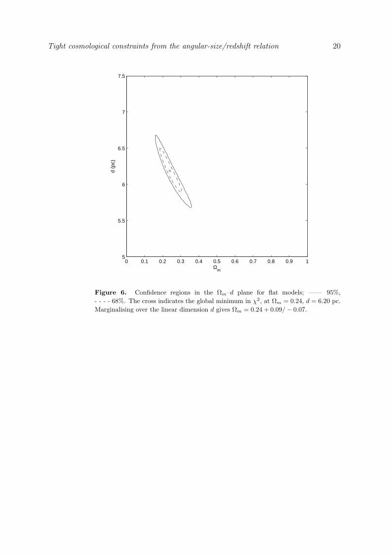
Tight cosmological constraints from the angular-size/redshift relation 20

0 0.1 0.2 0.3 0.4 0.5 0.6 0.7 0.8 0.9 15

5.5

6

6.5

7

7.5

Ωm

d (p

c)

Figure 6. Confidence regions in the Ωm–d plane for flat models; —— 95%,- - - - 68%. The cross indicates the global minimum in χ2, at Ωm = 0.24, d = 6.20 pc.Marginalising over the linear dimension d gives Ωm = 0.24 + 0.09/− 0.07.

Tight cosmological constraints from the angular-size/redshift relation 21

0 0.1 0.2 0.3 0.4 0.5 0.6 0.7 0.8 0.9 1−1

−0.9

−0.8

−0.7

−0.6

−0.5

−0.4

−0.3

−0.2

−0.1

0

Ωm

w

Figure 7. Confidence regions in the Ωm–w plane for flat models, marginalised overthe linear dimension d, where w is the quintessence parameter; —— 95%, - - - - 68%.The cross indicates the global minimum in χ2, at Ωm = 0.07, w = −0.44.