The Heavy Plough and the Agricultural Revolution in ...
61
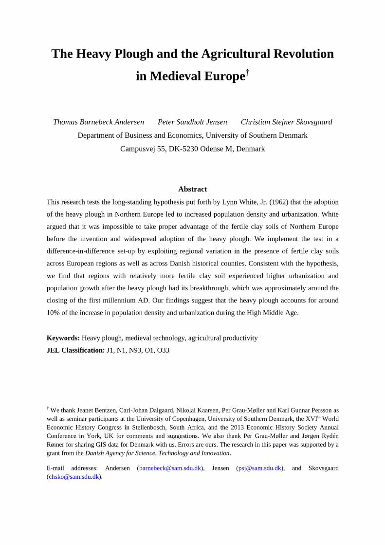
The Heavy Plough and the Agricultural Revolution in Medieval Europe † Thomas Barnebeck Andersen Peter Sandholt Jensen Christian Stejner Skovsgaard Department of Business and Economics, University of Southern Denmark Campusvej 55, DK-5230 Odense M, Denmark Abstract This research tests the long-standing hypothesis put forth by Lynn White, Jr. (1962) that the adoption of the heavy plough in Northern Europe led to increased population density and urbanization. White argued that it was impossible to take proper advantage of the fertile clay soils of Northern Europe before the invention and widespread adoption of the heavy plough. We implement the test in a difference-in-difference set-up by exploiting regional variation in the presence of fertile clay soils across European regions as well as across Danish historical counties. Consistent with the hypothesis, we find that regions with relatively more fertile clay soil experienced higher urbanization and population growth after the heavy plough had its breakthrough, which was approximately around the closing of the first millennium AD. Our findings suggest that the heavy plough accounts for around 10% of the increase in population density and urbanization during the High Middle Age. Keywords: Heavy plough, medieval technology, agricultural productivity JEL Classification: J1, N1, N93, O1, O33 † We thank Jeanet Bentzen, Carl-Johan Dalgaard, Nikolai Kaarsen, Per Grau-Møller and Karl Gunnar Persson as well as seminar participants at the University of Copenhagen, University of Southern Denmark, the XVI th World Economic History Congress in Stellenbosch, South Africa, and the 2013 Economic History Society Annual Conference in York, UK for comments and suggestions. We also thank Per Grau-Møller and Jørgen Rydén Rømer for sharing GIS data for Denmark with us. Errors are ours. The research in this paper was supported by a grant from the Danish Agency for Science, Technology and Innovation. E-mail addresses: Andersen ([email protected]), Jensen ([email protected]), and Skovsgaard ([email protected]).
Transcript of The Heavy Plough and the Agricultural Revolution in ...
The Heavy Plough and the Agricultural Revolution
in Medieval Europe†
Thomas Barnebeck Andersen Peter Sandholt Jensen Christian Stejner Skovsgaard
Department of Business and Economics, University of Southern Denmark
Campusvej 55, DK-5230 Odense M, Denmark
Abstract
This research tests the long-standing hypothesis put forth by Lynn White, Jr. (1962) that the adoption
of the heavy plough in Northern Europe led to increased population density and urbanization. White
argued that it was impossible to take proper advantage of the fertile clay soils of Northern Europe
before the invention and widespread adoption of the heavy plough. We implement the test in a
difference-in-difference set-up by exploiting regional variation in the presence of fertile clay soils
across European regions as well as across Danish historical counties. Consistent with the hypothesis,
we find that regions with relatively more fertile clay soil experienced higher urbanization and
population growth after the heavy plough had its breakthrough, which was approximately around the
closing of the first millennium AD. Our findings suggest that the heavy plough accounts for around
10% of the increase in population density and urbanization during the High Middle Age.
Keywords: Heavy plough, medieval technology, agricultural productivity
JEL Classification: J1, N1, N93, O1, O33
† We thank Jeanet Bentzen, Carl-Johan Dalgaard, Nikolai Kaarsen, Per Grau-Møller and Karl Gunnar Persson as
well as seminar participants at the University of Copenhagen, University of Southern Denmark, the XVIth
World
Economic History Congress in Stellenbosch, South Africa, and the 2013 Economic History Society Annual
Conference in York, UK for comments and suggestions. We also thank Per Grau-Møller and Jørgen Rydén
Rømer for sharing GIS data for Denmark with us. Errors are ours. The research in this paper was supported by a
grant from the Danish Agency for Science, Technology and Innovation.
E-mail addresses: Andersen ([email protected]), Jensen ([email protected]), and Skovsgaard

1
1. Introduction
As of the 9th century to the end of the 13th century, the medieval European economy
underwent unprecedented productivity growth (White 1962; Pounds 1974; Langdon, Astill
and Myrdal 1997). The period has been referred to as the most significant agricultural
expansion since the Neolithic revolution (Raepsaet 1997). In his path-breaking book,
“Medieval Technology and Social Change”, Lynn White, Jr. argues that the most important
element in the “agricultural revolution” was the invention and widespread adoption of the
heavy plough (White 1962).
The earliest plough, commonly known as the ard or scratch-plough, was suitable for the soils
and climate of the Mediterranean; it was, however, unsuitable for the clay soils found in most
of Northern Europe, which “offer much more resistance to a plough than does light, dry
earth” (White 1962, p. 42). The consequence was that north European settlement before the
Middle Age was limited to lighter soils, where the ard could be applied. The heavy plough
and its attendant advantages may have been crucial in changing this. More specifically, heavy
ploughs have three function parts that set them apart from primitive ards. The first part is an
asymmetric ploughshare, which cuts the soil horizontally. The second part is a coulter, which
cuts the soil vertically. The third part is a mouldboard, which turns the cut sods aside to
create a deep furrow (Mokyr 1990; Richerson 2001). The mouldboard is the part of the heavy
plough from which its principal advantages on clay soils derive. The first advantage is that it
turns the soil, which allows for both better weed control on clay soil in damp climates and
incorporation into the soil of crop residues, green manure, animal manure or other substances
(Richerson 2001; Guul-Simonsen et al. 2002). The second advantage is that mouldboard
ploughing produced high-backed ridges, which contributed to more efficient drainage of clay
soils. The ridges also allowed for better harvests in both wet and dry seasons. The third
advantage is that the heavy plough handles the soil with such violence that cross-ploughing is
not needed, thus freeing up labor time. Hence by allowing for better field drainage, access to
the most fertile soils, and saving of peasant labor time, the heavy plough stimulated food
production and, as a consequence, “population growth, specialization of function,
urbanization, and the growth of leisure” (White 1962, p. 44).

2
While White’s work is certainly not without its critics among historians,1 others have
followed his lead. Mokyr (1990, p. 32), for example, writes that it “has taken the combined
geniuses of Marc Bloch (1966) and Lynn White (1962) to make historians fully recognize the
importance of the heavy plow, or carruca.” Landes (1998, p. 41) notes that the heavy plough
“opened up rich river valleys, turned land reclaimed from forest and sea into fertile fields, in
short it did wonders wherever the heavy, clayey soil resisted the older Roman wooden scratch
plow, which had worked well enough on the gravelly soils of the Mediterranean basin.” In
fact, the historiography of medieval technology and its impacts contains a large amount of
circumstantial evidence pointing towards a crucial role of the heavy plough for medieval
economic development (see Poulsen 1997; Jensen 2010; Pounds 1974). The heavy plough
hypothesis has also been perpetuated in a leading textbook on “Civilization in the West”,
where students are told that the heavy plough “increased population in the heavy soil areas
north of the Alps” (Kishlansky et al. 2010, p. 201). Yet to this date there exists no rigorous
quantitative evidence on its impact. This present research aims to fill this gap.
We adopt a difference-in-difference type strategy to test the impact of the introduction of the
heavy plough. We exploit two sources of variation: time variation arising from the adoption
of the heavy plough in Europe in the Middle Age and cross-sectional variation arising from
differences in regional suitability for adopting the heavy plough. This basically allows us to
compare changes in economic development, as measured by urbanization and population
density, in the post-adoption period relative to the pre-adoption period between regions that
were able to benefit from the heavy plough and regions that were not. Our sample contains
316 regions and, to avoid confounding our analysis with the devastating impact of the Black
Death, our window of observation is AD 500-1300. We implement our test under two
alternative assumptions. The first assumption is that we know exactly when the diffusion of
the plough took off in earnest. Under this assumption, a non-flexible model is appropriate.
The alternative assumption is that the exact date is unknown but that it happened after 500. In
this case a flexible model is called for as it allows us to assess when the plough began to have
a detectable effect on our outcome variables for each century of the Middle Age. As a
supplement to the flexible specification, we also apply rolling regressions to further
investigate the timing of the breakthrough of the heavy plough.
1 See Roland (2003) or Worthen (2009) for expositions of some of the criticism and for assessments of the
enduring influence of Lynn White, Jr.

3
While the European data support the heavy plough hypothesis, these data are likely to suffer
from measurement error. We have therefore constructed a new dataset for historical Danish
counties with more precise measures for both urbanization and fertile clay soils. The Danish
data allow us to test the hypothesis on an independent high-quality dataset.
We find evidence strongly consistent with White’s hypothesis. With respect to the European
sample, our estimations show that the heavy plough accounted for around 10% of the
increase in population density and urbanization in the High Middle Age. The empirical
evidence also largely confirms the historiographical evidence about the timing of the
introduction and breakthrough of the heavy plough in medieval Europe. We subject these
findings to a number of checks. For instance, we show that our results are robust to
reasonable alterations of our measure of soil suitability for using heavy ploughs;
unreasonable alterations of the soil suitability measure, however, imply a vanishing impact.
Specifically, we conduct a placebo-type experiment using suitability for growing the potato.
This is a crop brought to Europe from the Americas in the Age of Discovery, which strongly
influenced urbanization and population density in potato suitable areas after its introduction
(Nunn and Qian 2011). Consistent with our identification strategy, potato suitability has no
significant effect on local economic development in our sample period. With respect to the
Danish sample, we also find strong evidence that counties with higher shares of fertile clay
soils experienced greater urbanization in the medieval epoch.
Overall, our research complements existing accounts from the historiography of medieval
technology with rigorous quantitative evidence. To the best of our knowledge, we provide the
first econometric test of the heavy plough hypothesis. Our empirical strategy which exploits
on exogenous variation in fertile clay soil in a difference-in-difference setup deals with the
concern about reverse causality raised by Hilton (1963) in his critical review of White’s
book. Second, we provide evidence that increased agricultural productivity can be a powerful
driver of economic development in an agrarian economy. Third, we provide a clear historical
example of what Acemoglu, Johnson and Robinson (2005a) call the “sophisticated geography
hypothesis.” This hypothesis holds that particular geographical characteristics that were not
useful (or even outright harmful) for successful economic performance at some point in time
may turn out to be beneficial later on. The reason is that certain technological inventions may
benefit particular geographical characteristics. In the present case, the heavy plough (the
technological invention) benefitted areas endowed with fertile clay soils (the geographical

4
characteristic). Finally, our paper speaks to the literature on “the little divergence” which
stresses regional differences in development within Europe (e.g. Broadberry, van Leuwen and
van Zanden 2012; Baten and van Zanden 2008). In particular, these authors stress that living
standards became higher in north-west Europe compared to Mediterranean Europe after 1500.
The paper considers a factor that contributed to regional differences in growth trajectories
within Europe; it also demonstrates regional differences in development within a particular
European country, Denmark. In this way, the paper explores economic geography aspects
usually not discussed in “the little divergence” literature.
The rest of the paper is organized as follows. Section 2 contains a detailed discussion of the
advantages of the heavy plough on clay soils, and it provides historical background for the
introduction and diffusion of the heavy plough in Europe. Section 3 outlines the empirical
model. Section 4 describes our data. Sections 5 and 6 present the results. Section 7 concludes.
2. Background
This section first explains the advantages of using heavy ploughs on clay soil. Understanding
these advantages is important as they form the foundation of the heavy plough hypothesis.
Second, we review the existing evidence on the diffusion of the plough in Europe. Doing so
provides us with knowledge that helps guide our econometric strategy.
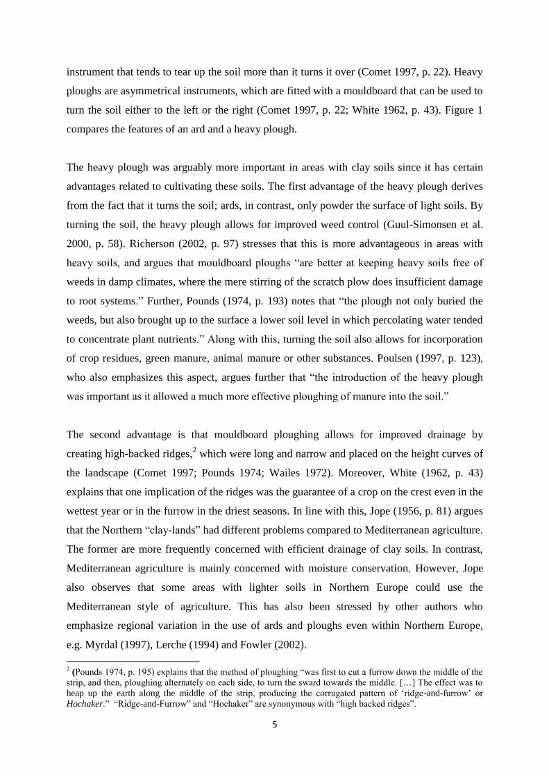
Figure 1: The ard (a) and the heavy plough (b). Source: Fowler (2002).
2.1 Advantages of the heavy plough
The earlier ploughs—known as ards or scratch ploughs—are almost as old as agriculture
itself, and they were probably already in use by 4000-6000 BC in ancient Mesopotamia (Soil
& Tillage Research 2007, p. 2). An ard, which exists in different varieties, is a symmetrical
5
instrument that tends to tear up the soil more than it turns it over (Comet 1997, p. 22). Heavy
ploughs are asymmetrical instruments, which are fitted with a mouldboard that can be used to
turn the soil either to the left or the right (Comet 1997, p. 22; White 1962, p. 43). Figure 1
compares the features of an ard and a heavy plough.
The heavy plough was arguably more important in areas with clay soils since it has certain
advantages related to cultivating these soils. The first advantage of the heavy plough derives
from the fact that it turns the soil; ards, in contrast, only powder the surface of light soils. By
turning the soil, the heavy plough allows for improved weed control (Guul-Simonsen et al.
2000, p. 58). Richerson (2002, p. 97) stresses that this is more advantageous in areas with
heavy soils, and argues that mouldboard ploughs “are better at keeping heavy soils free of
weeds in damp climates, where the mere stirring of the scratch plow does insufficient damage
to root systems.” Further, Pounds (1974, p. 193) notes that “the plough not only buried the
weeds, but also brought up to the surface a lower soil level in which percolating water tended
to concentrate plant nutrients.” Along with this, turning the soil also allows for incorporation
of crop residues, green manure, animal manure or other substances. Poulsen (1997, p. 123),
who also emphasizes this aspect, argues further that “the introduction of the heavy plough
was important as it allowed a much more effective ploughing of manure into the soil.”
The second advantage is that mouldboard ploughing allows for improved drainage by
creating high-backed ridges,2 which were long and narrow and placed on the height curves of
the landscape (Comet 1997; Pounds 1974; Wailes 1972). Moreover, White (1962, p. 43)
explains that one implication of the ridges was the guarantee of a crop on the crest even in the
wettest year or in the furrow in the driest seasons. In line with this, Jope (1956, p. 81) argues
that the Northern “clay-lands” had different problems compared to Mediterranean agriculture.
The former are more frequently concerned with efficient drainage of clay soils. In contrast,
Mediterranean agriculture is mainly concerned with moisture conservation. However, Jope
also observes that some areas with lighter soils in Northern Europe could use the
Mediterranean style of agriculture. This has also been stressed by other authors who
emphasize regional variation in the use of ards and ploughs even within Northern Europe,
e.g. Myrdal (1997), Lerche (1994) and Fowler (2002).
2 (Pounds 1974, p. 195) explains that the method of ploughing “was first to cut a furrow down the middle of the
strip, and then, ploughing alternately on each side, to turn the sward towards the middle. […] The effect was to
heap up the earth along the middle of the strip, producing the corrugated pattern of ‘ridge-and-furrow’ or
Hochaker.” “Ridge-and-Furrow” and “Hochaker” are synonymous with “high backed ridges”.

6
The third advantage emphasized by White (1962, p. 43) was that the heavy plough “handled
the clods with such violence that there was no need for cross-ploughing.” This meant less
work effort for a given amount of land, thus increasing the productivity of farmers.
Finally, the use of the heavy plough on light sandy soils may lead to a gradual destruction of
the soils in the longer run (Henning 2009). Some evidence on the relative advantage of the
heavy plough on clay soils exists in the form of modern mouldboard ploughing tests. These
tests reveal that mouldboard ploughing increases crop yields on clay soils with considerably
higher clay content in the subsoil than the topsoil (Guul-Simonsen et al. 2002, p. 64). We will
use this fact in the construction of our empirical measures below.
2.2 Origin and diffusion of the heavy plough3
Establishing the origin and timing of diffusion of the heavy plough is no easy task. It is,
however, an important one because our empirical strategy relies on comparing European
regions before and after the widespread adoption of the heavy plough. For this reason, we
need to carefully examine the research that sheds light on this issue. We will consider both
the archaeological research on plough marks, plough remains and figurative representations
as well as the linguistic evidence. As will be discussed in detail below, the existing evidence
suggests that the heavy plough may have been introduced in some areas before AD 1000, but
its breakthrough or widespread adoption—which is what should really concern us—seems
only to have started in earnest around AD 1000.
Comet (1997) envisions the gradual evolution from ard to heavy plough as follows: “First the
ancient ard was fitted with a coulter and a wheeled fore-carriage, which made it heavier and
required more draught animals. The farmer could lean on the carriage, so that the ard became
easier to steer and could be tilted to one side. With addition of a mouldboard and the
development of asymmetric shares, the transition to the plough was made.” According to this
view, the development of the heavy plough is likely to have been gradual. This is one reason
why it is difficult to pinpoint its exact origin and diffusion by relying on the existing
evidence. Nonetheless, attempts to do so have been made. White (1962), for example, argues
3 The time periods for the introduction and breakthrough across modern states are discussed in Appendix F
based on various sources. The time periods refer to the approximate time period of the breakthrough or in some
cases the century of introduction.
7
that Slavs may have introduced it, and that it therefore diffused from east to west starting in
the late 6th
century. Some of the evidence discussed below is in line with the view that the
heavy plough was introduced in some parts of South Eastern Europe. Others have argued that
it was invented by Germanic tribes and spread to Eastern Europe as part of the eastern
expansion of the Germanic tribes (Barlett 1993; Piskorski 1999).
For the period before AD 500, Manning (1964, p. 57) notes that there is evidence for bow
ards being used in the Iron Age and Roman Period in Scandinavia, the Rhineland, Britain and
Italy. According to Manning, this distribution is wide enough for us to assume that it was the
normal type of plough throughout Europe at the time. Fowler (2002, p. 203) argues that the
bow ard remained the plough available to most farmers in England throughout the first
millennium AD, and that it remained important across Europe. Moreover, the evidence from
the British Isles suggests that the heavy plough only came in use at the end of the first
millennium. Other historians hold similar views. Fussell (1966, p. 178), for example,
concludes that for Europe as whole much evidence suggests that the heavy plough only came
into general use as of the 11th
century and onwards. Similarly, but focusing on Northern
Europe, Heaton (1963, p. 100) argues that after AD 1000 the (wheeled) heavy plough drawn
by eight oxen “was used more and more to turn the heavy clay lands which became available
with the clearing of some forest areas.” We now turn to a more detailed discussion of the
various strands of evidence.
Plough marks
The earliest evidence that has been interpreted as indicating the use of a heavy plough comes
from the Iron Age settlement Feddersen-Wierde in Northern Germany (Hardt 2003; Larsen
2011; Wailes 1972). The furrows discovered at Feddersen-Wierde can be dated back to the
first century BC, but there is some doubt that a heavy plough in fact produced them.
First, Larsen (2011, p. 83) notes that it may be difficult to distinguish the furrows from heavy
ploughs and certain types of ards. In a similar vein, Wailes (1972, p. 161) argues that the
furrows could have been produced by “skillfull tilting of a heavy ard.” The presence of
symmetrical shares found at Feddersen-Wierde corroborates the argument of Wailes (1972)
that the furrows may indeed be ard marks.

8
Second, as discussed above, mouldboard ploughing is known to create fields with high-
backed ridges. Thus, a stronger indicator of the breakthrough of the heavy plough is the
presence of high-backed ridges, which—in contrast to the aforementioned furrows—only a
heavy plough could have created (Poulsen 1997, p. 127). Yet there are no high-backed ridges
at Feddersen-Wierde (Grau-Møller 1990). High-backed ridges have been observed and dated
in several countries, including Britain, Denmark, Germany, Netherlands, and Sweden. The
earliest of these are dated to around AD 1000 (Grau-Møller 1990). Thus, the evidence on
high-backed ridges favours the view that the breakthrough of mouldboard ploughs took place
around AD 1000. This conclusion is in line with the view of Fowler (2002), Fussel (1966),
and others as stated above.
Plough remains
Heavy ploughs and ards consist of different parts, cf. Figure 1. The most prominent part is the
mouldboard, which therefore indicates most clearly the existence of heavy ploughs. Coulters
and shares are also of interest, but as discussed below there are important reasons for
doubting whether or not these parts give definite evidence for the presence of heavy ploughs.
The archaeological literature discusses discoveries and dating of mouldboards, shares and
coulters, and next we discuss the discoveries of these three parts in turn.
Mouldboards: Unfortunately, few mouldboards have survived. Larsen (2011) discusses two
from Denmark, but they have not been dated. According to Fowler (2002), for the British
Isles there is no evidence of mouldboards for the first millennium AD.
Coulters: Lerche (1994) provides an overview of findings of coulters, which for Hungary
and the Danube area can be dated to the first century AD. In Britain and Ireland, coulters that
date back to the Roman era have been found; in Germany, coulters that date back to the
period 3rd
to 6th
century AD have been found. However, as pointed out by among others
Comet (1997) and Fowler (2002), the presence of coulters does not imply the mouldboard
plough, as coulters were also attached to ards.
Shares: These are of particular interest as they indicate whether the instrument was
symmetrical or asymmetrical. An asymmetrical share would be consistent with the existence
of mouldboard ploughs.

9
The shares found in Feddersen-Wierde are all symmetrical (Felgenhauer-Schmidt 1993, p.
167). This indicates the use of ards rather than mouldboard ploughs. The earliest evidence of
asymmetrical shares comes from Roman Britain where three such parts have been found
(Manning 1964, p. 65; Wailes 1972, p. 163). This is consistent with the existence of
mouldboard ploughs, but it has been suggested by Wailes (1972, pp. 163-64) that
asymmetrical ards have existed. Moreover, Manning (1965) argues that the bow ard was the
normal plough of the period, as noted above. More systematic evidence on the evolution of
shares is given in Henning (1987) for Southeastern Europe, which encompasses parts of the
Balkans as well as Hungary and Slovakia. Henning shows that from the 3rd
to the 6th
century,
there is no systematic asymmetry in the shares found, but concludes that for the period from
the 7th
to the 10th
century there is a strong “overweight of left-sided asymmetry” (1987, p.
55). This is consistent with White’s view that Slavic tribes had the heavy plough from around
AD 600. Other asymmetrical shares are covered in Lerche (1994, Chapter 9), where German
and Czech findings of ploughshares dating back to the 11th
century or later are discussed, and
also in Larsen (2011), who reviews the evidence for Denmark and parts of present-day
Sweden and north Germany. These asymmetrical shares can all be dated to the High Middle
Age or later.
Based on the British evidence, Fowler (2002, p. 203) concludes that “cultivating implements
with coulters and large shares, but no proven mouldboard, were known in third- and fourth-
century Southern Britain, and were probably the source of the similar implements attested in
Western Britain and Ireland in the second half of the millennium.” The existing
archaeological evidence therefore does not provide definitive evidence of the introduction of
the heavy plough, although the evidence provided by Henning (1987) is consistent with a
widespread adoption of asymmetrical heavy ploughs in the 7th
-10th
century in some areas.
Figurative representations
Depictions may indicate when a technology had its breakthrough, though important caveats
are that it sometimes is difficult to date figurative representations, and that it is not always
clear whether an artist copied what “he saw, or rather what had inspired previous work of art
or studio models” as argued by Duby (1968, pp. 390-391).
The earliest depictions are mentioned by Astill (1997, p. 201), who points to seven English
manuscript illustrations of ploughing dating back to the late 10th
and 11th
century. Another

10
early and often cited figurative representation is found on the Bayeux Tapestry sewn in
Normandy or England the late 11th
century (Grau-Møller 1990; Fowler 2002; Jensen 2010).
Later figurative representations are given in Duby (1968, pp. 390-391), who reproduces a
drawing from the 12th
century and a painting from the 15th
century of a heavy plough from
France, and who observes that the construction has not changed much over time in the two
illustrations. Still other depictions of ploughing implements are found in the form of church
paintings. For example, Larsen (2011) dates paintings depicting heavy ploughs to the 15th
or
16th
century for the case of Denmark. Thus, to the extent that the dates of the figurative
representations are informative of the breakthrough of heavy ploughs, the earliest date seems
to be the late 10th
century.
Linguistic evidence
As already mentioned, White (1962, pp. 49-50) argues that the Slavic tribes introduced the
heavy plough around AD 568. This conclusion was reached by considering evidence that
indicated that a word for plough and many associated terms existed in all of the three Slavic
linguistic groups. More specifically, White (1962, p. 50) reasons that “since the Slavic
vocabulary surrounding plug probably would have developed rapidly, once the Slavs got the
heavy plough, we have no reason to date its arrival among them very long before the Avar
Invasion of 568.” He also points out that the word ‘plough’ first appears in written form in
643 in north Italy as the Lombardian ‘plovum’ in the Langobaridan Edictus Rothari.4 For
Southwest Germany, the Lex Alemannorum shows that the word ‘carruca’ had come to mean
a plough with two wheels in front by the 8th
century. There is also written evidence for a
heavy plough in Wales in the 10th
century in the laws of Hywel Dda (White 1962, pp. 50-51).
Puhvel (1964, pp. 180-181) notes that the word for plough (plogr) does not appear in old
Norse before AD 1000, whence it probably spread to 11th
century England where ‘plog’ or
‘ploh’ replaced the older word ‘sulh’.5
Summing Up
4 The word “plaumorati” also appears in a text by Pliny the elder from the 1
st century. White (1962) says that
this word is unintelligible, but if it is replaced by ‘ploum rati’, we have the first appearance of the non-classical
word ‘plough’, but he later refers to this as “the questionable emendation of the Pliny text’s plaumorati.”
Further, the exact nature of Pliny’s plough has been questioned. Wailes (1972, p. 163) says that it did not
necessarily have a mouldboard as contented by other authors. Rapsaet (1997, p. 43) notes that Pliny’s plough is
often believed to be a wheel ard. 5 White (1962, pp. 53-54) argues that the plough was introduced from Denmark to England in the late 9
th and
early 10th
centuries. Myrdal (1997, p. 155) accepts this possibility, but notes that the diffusion could have been
in the opposite direction with the connection being north England and Norway.
11
Our discussion of the evidence demonstrates that there are conflicting time periods for the
introduction and breakthrough of heavy ploughs. As explained above, a view held by many
historians, including Heaton (1963), Fowler (2002), Fussel (1966), Wailes (1972) and
Poulsen (1997), is that the breakthrough happened from around AD 1000 onwards. In
Appendix F we provide further evidence, which shows that for many countries the
breakthrough is believed to have happened around this time. Moreover, this particular dating
(AD 1000) is corroborated by the presence of high-backed ridges from around this time. The
figurative evidence is also in line with the view of the breakthrough starting from AD 1000.
Further, even if heavy ploughs existed earlier, ards seem to have been more common in the
earlier periods, as emphasized by Manning (1965) and Fowler (2002).6
In sum, we use the AD 1000 timing below. However, since there is ample uncertainty
regarding this date, we also use estimation methods that allow for an uncertain breakthrough
date.
3. Empirical strategy
As explained in Section 1, our identification strategy follows the logic of the standard
difference-in-difference estimator. We exploit both the time variation arising from the
adoption of the heavy plough in the Middle Ages and the cross-sectional variation arising
from differences in regional suitability for adopting the heavy plough.7 The European regions
we use are the Nomenclature of Territorial Units for Statistics (NUTS) regions. We have
chosen NUTS level 2, because it gives a detailed and relatively uniform subdivision of
Europe. At this level, Europe is divided into 316 regions.8 Given our historical period of
interest, we focus on the period 500-1300.9 As mentioned in section 1, we also implement the
test on Danish data, but we defer detailed discussion of these to Section 6.
6 This is in line with Landes (1998, p.41) who stresses that the heavy plough went back earlier, but were only
taking widely into use from 1000 AD. 7 A similar strategy is applied by Nunn and Qian (2011) in their evaluation of the impact of the introduction of
the potato from the new to the old world and by Acemoglu et al. (2005b) in their evaluation of the gains from
Atlantic trade opportunities. 8NUTS regions are divided into 5 levels. Level 0 is the country level, level 1 mixes the regional and country
level, levels 2-4 contain the regional level, but level 4 only exists in Poland; thus, the degree of division
increases with the level. The divisions are in most cases based on present national administrative subdivisions.
Figure C1 in Appendix C shows the NUTS 2 division. 9 We begin our investigation before the (presumed) widespread adoption of the heavy plough, and we end
before the medieval economy was hit by the devastating plague.
12
We implement our test under two alternative assumptions. The first assumption is that we
know when the diffusion of the plough took off in earnest. As discussed above, the evidence
indicates that this happened from around AD 1000. We therefore estimate non-flexible
models in which the post-treatment period is AD 1000 onwards. The second assumption is
that the exact date is unknown but that it happened sometime after AD 500. In this case a
flexible model is the natural complement to the non-flexible model. With a flexible approach
we can assess when the plough began to have a noticeable effect on agricultural productivity.
As a supplement to the flexible models, we also apply rolling regressions of 400-year periods
to further investigate the timing of the breakthrough of the heavy plough.
3.1 Non-Flexible Model
Our non-flexible model is given by the following equation:
In the equation, denotes time (centuries from 500-1300), denotes NUTS-regions, is
economic development, is an interaction between the share of
plough suitable area10
in region and a dummy variable being 1 from AD 1000
onwards, thus indicating our assumption that the heavy plough became widespread after this
date. Our main coefficient of interest is , which indicates the causal impact of having plough
suitable area.11
A positive coefficient would be in line with the hypothesis that the heavy
plough mattered for economic development. The remaining variables are control variables,
, interacted with century dummy variables, regional fixed effects, , time fixed effects,
,
and the error term, . We postpone the discussion of control variables to Section 4.
3.2 Flexible Model
The flexible model is described by:
10
See description in Section 4.1 11
Since we have no knowledge of the take-up rate of the heavy plough, is an intention-to-treat (ITT) type
estimate.

13
where the crucial difference from equation (1) is that we obtain an estimate for all centuries
and hence let the data ‘speak’ as to when the effect of the heavy
plough becomes traceable. All the other variables are the same as in the previous section.
This model estimates the excess effect of having fertile clay soil in period compared to AD
500.
4. Data
4.1 Main variables
In order to estimate the above equations, we need several data series. First and foremost, we
need a measure of regional economic development and a measure of fertile clay soil.
We employ two different measures of economic development: urbanization and population
density. The focus on urbanization is warranted by the fact that historians have linked the
heavy plough and urbanization (e.g., White 1962; Jensen 2010). Moreover, Nunn and Qian
(2011) and Pounds (1974) argue that urbanization is closely related to per capita income; and
Acemoglu et al. (2005a, p. 408) argue that only societies with a certain level of agricultural
productivity and a relatively developed system of transport and commerce can sustain large
urban centers (see also Diamond 1998). The heavy plough arguably increased agricultural
productivity and the need for markets, and it therefore allowed for urbanization. Besides,
productivity increases in the agricultural sector may have spawned migration to the urban
sector (Nunn and Qian 2011).12
Pounds (1974, p. 103) argues that evidence does indeed
suggest that migration to towns and cities was taking placing in the Middle Ages. The focus
on population density is usually rationalized by invoking Malthusian thinking (Nunn and
Qian 2011). In a Malthusian model, a one-off positive productivity shock—as brought about
by the heavy plough, say—is fully offset by fertility increases. Income per person may
increase in the short run; in the long run, however, any such increase is completely offset by
increased fertility. In the long run, income per person therefore stays constant and population
levels are permanently higher (Ashraf and Galor 2011).
With respect to urbanization, we construct this measure using historical maps from EurAtlas
for the period 500-1300. We build on Pounds (1974) in that he suggests using number of
cities and towns as an indicator of economic growth for the medieval period. EurAtlas
12
Pounds (1974) argues that all towns had an agricultural sector, and in this way, they may have benefitted
directly from the heavy plough.

14
provides information on the locations of cities by century. Cities were towns that had
achieved some importance in the sense that they had become the seat of a bishop (Pounds
1974, p. 101). Specifically, we use the number of cities per square kilometer.13
Moreover,
Bairoch (1988, pp.135-136) stresses that the period from around 900 to 1300 was a period of
rapid urban growth in Europe, and points out that the way this happened was partly by “the
creation of a great many new urban centers” and partly by the expansion of existing cities. He
produces estimates of the number of cities from 800 to 1300 for Europe as a whole, and
shows that both the number of cities and urban populations more than tripled in this period.
This suggests that in the historical period we cover, the number of cities follow growth in
urban population, and we therefore regard our measure as the best proxy available. We also
note that an advantage of this measure is that it tracks the transition from insignificant
villages to cities which took place in the period under study. Another advantage is that we do
not have to make an arbitrary population-based cut-off of what constitutes a city. A
disadvantage of this measure is obviously that we do not capture the growth of existing
cities.14
With respect to population density, obtaining this at the regional level is possible but not
unproblematic for reasons discussed below. We use gridded population density data from the
HYDE database,15
which was developed under the authority of the Netherlands
Environmental Assessment Agency. The measure is based on historical national population
data such as McEvedy and Jones (1978), Livi-Bacci (2007), Maddison (2001) and Denevan
(1992), supplemented by historical subnational data (Klein Goldewijk et al. 2010; 2011). The
first problem with these data is that for periods before the 18th
century they are not
constructed on the basis of national censuses. The first census in continental Europe was that
of Sweden in 1749, and data before this time are scarce (McEvedy and Jones 1978). The
second problem is that to construct gridded data, the researchers who produced the HYDE
database relied on various geographical weights. Still, they stress that these weights are
unchanged over time, and that only population density and the amount of agricultural area
changes over time. We calculate the average population density at the NUTS 2 level for each
century of our observation period.16
While this variable is constructed, it correlates positively
13
A similar measure of urbanization has been used by historians such as Beresford (1967) for England. 14
Available data on the size of cities by Bairoch et al. (1988) are unfortunately very sparse for the period before
1300. 15
Klein Goldewijk (2010), Hyde Database: http://themasites.pbl.nl/en/themasites/hyde/index.html 16
For an example, see Figure C1 in Appendix C

15
with our measure of urbanization.17
Given that our urbanization indicator is not a constructed
measure, this suggests that the constructed population density measures do to some extend
track economic development.
We also need a measure on how suitable different soils are to the use of the heavy plough.
According to White (1962) and others, it was areas with clay soils that gained from adapting
the heavy plough. Yet none of the writers in the historiographical tradition provide precise
definitions of “clay soils”, “heavy clay soils” or “heavy soils”. A challenge is therefore to
find a soil type that fits this description in commonly used soil classification systems. We
employ the European Soil database, which builds on the classification system of the Food and
Agriculture Organization (FAO). In this system the soil type known as luvisol fits most
closely the description given in the historiographical literature. Luvisol is rich in clay, has
higher clay content in the subsoil than in the topsoil, and its soil profile implies that clay
content increases with soil depth (FAO 2006, p. 86; Louwagie et al. 2009).18
As noted in
Section 2.1, this type of soil has been shown to benefit from mouldboard ploughing in terms
of crop yields.
Fertile luvisol is much more common in Northern Europe than in Southern Europe. Their
geographical locations fit closely with the areas where historians have pointed to the presence
of “clay soils”, “heavy soils” or “heavy clay soils”, and where they believe mouldboard
ploughs would have been beneficial. At this general level, Hodgett (1974, p. 16) argues that
the temperate zone of Europe contained much more “heavy clay soil” than did the
Mediterranean zone, though some heavy soils exist “even in Southern Europe”. For the case
of Denmark, many historians have pinpointed the areas dominated by luvisol as areas with
“clay soils”, “heavy soils” and “heavy, moraine clay” (Jensen 1979, p. 20; Andersen and
Nielsen 1982, pp. 62-63; Jensen 2010, p. 136). Pounds (1974, p. 112) argues that “the heavy
plough, with its coulter and mouldboard” was “essential if the heavy clays of the Polish plain
were to be cultivated.” And luvisol is in fact the dominant soil in Poland; cf. Figure C2,
Appendix C. Hodgett (1974, p. 16) argues that the heavy plough would be useful on the
“heavy soils” in the valley of the river Po. White (1962, p. 42) also notes that the heavy
plough was in use in the Po Valley in later times for reasons of soil and climate. In fact, in the
17
The correlation coefficient is 0.43. 18
This is a result of pedogenetic processes, which leads to a so-called argic subsoil horizon. The presence of an
argic subsoil horizon requires that the clay content increases sufficiently with depth
(http://eusoils.jrc.ec.europa.eu/library/Maps/Circumpolar/Download/39.pdf).

16
region of Lombardy, which dominates the area of the Po Valley, luvisol is highly prevalent.19
In line with this, Parain (1966, p. 374) notes that heavy ploughs were used on the clay soils of
Lombardy. In section 6 below, we return to the challenge of measuring clay soils by using
alternative measures for the case of Denmark.
A concern regarding the use of data based on 20th
century soil maps is that they may not
represent the composition of soils in the Middle Ages. Many authors in the historiographical
tradition write on the presumption that present-day soil maps are informative of past
conditions. Comet (1997, p. 27), for example, argues that the “fundamental composition of
soils in Northern France has probably not changed much since the eleventh century.” This is
not an unreasonable presumption as the available evidence does indicate that heavy clay soils
appear to have been formed long before the Middle Ages.20
According to Alexandrovskiy
(2000, p. 238), for instance, the steppe stage with chemozem soils was replaced by a forest
stage with luvisol in regions of Russia 3000 years ago and in Central Europe some 11,000
years ago. For the case of Denmark, Milthers (1925, p. 23) notes that the clay soils formed
during the ice age.
On this background, we identify the areas with high prevalence of “luvisol” as our baseline
measure for clay soil. But in order to identify the areas that would benefit from adapting the
heavy plough we need a second condition: We have to adjust for the quality of the soil for
growing plough positive crops, such as wheat, barley and rye.21
We must do so since areas
with infertile, clay soil are unlikely to benefit from the heavy plough. Also, using only data
for plough friendly crops would not distinguish between areas that benefitted from using
heavy ploughs or scratch ploughs. The aforementioned crops were also the most common in
the High Middle Age (Pounds 1974).
In effect, we construct our measure of the usefulness of the heavy plough from two sources: a
soil raster map from the European Soil Database as mentioned above and a raster map
indicating the suitability for growing plough positive crops. The suitability map comes from
the Global Agro-ecological Assessment 2002 by FAO which classifies the soil using
19
A soil map has been constructed for the subregion of Lombardy. In this region, luvisol is the most common
type of soil (see http://www.ersaf.lombardia.it/upload/ersaf/suoli/eng/soilmap.asp). 20
Nevertheless, Comet (1997) warns that it would be wrong to take continuity for granted. For example, he
notes problems of soil erosion, which was facilitated by clearing of land. 21
See Pryor (1985) for a discussion of which staple crops are plough positive. Pryor also discusses the need for
the right climatic/geographical conditions for the usefulness of the plough.

17
thresholds on a soil suitability index denoted by SI.22
The corresponding classification
divides soil suitability into categories from “very marginal” to “very high”, see appendix C
for details. The measure, which we denoted PloughFraction, is constructed as the fraction of
the area of each region which contains luvisol with SI greater or equal to a certain threshold
for a plough positive crop.23
We construct a baseline measure of PloughFraction using
luvisol with for wheat. In terms of soil suitability classification, this corresponds to
using luvisol with at least good suitability for growing wheat, but we also investigate other
crops and different thresholds for SI.24
Since our measures are a function of SI, a clearer
notation is PloughFraction(SI), and we therefore denote our baseline measure by
PloughFraction(55), cf. footnote 24. In some estimations we also include areas with (fertile)
gleysol. This is a wetland soil (FAO, 2006) and described as poorly drained by Edwards
(1990, p. 50). PloughFraction(55) is visualized in Figure 2. This map confirms that more
plough suitable land is found in Northern Europe and the northern parts of Italy.25
Figure 2: Distribution of “PloughFraction(55)” in Europe
22
Again we need to justify the use of present-day suitability data. In Figure C3 in Appendix C we show a map
of wheat suitability and a description of the suitability index. Figure D1 confirms a positive correlation between
historic wheat production and our wheat suitability measure based on present-day FAO data. Moreover, sub-
national data from Denmark confirms a relation between yields and soil suitability for the three crops
considered, see appendix D. 23
Due to uncertainty we drop regions where more than 20% of the soil is not defined. 12 regions are dropped in
this regard but including these regions only strengthens our results. 24
PloughFraction can be written in precise terms in the following way: Let F be the distribution function for
luvisol, and let G the distribution for suitability, then our measure of usefulness of the heavy plough is
PloughFraction(SI ) =1luvisol>0éë ùû
×1suitability>SIéë ùû
dF dGòòArea
,
where 1[ ] is the indicator function and SI is the suitability index threshold level. In most estimations, SI = 55,
which is the definition of “good suitability”; however, we also run estimations with “medium suitability”,
corresponding to SI = 40 and “high suitability” corresponding to SI = 70. See Appendix C for further details. 25
The map does not change substantially if areas with fertile gleysol are included.
18
4.2 Control Variables and threats to identification26
A first step in controlling for potentially omitted factors is to add regional fixed effects and
time dummy variables for each century. Regional fixed effects capture time-invariant
characteristics such as soil quality and other geographical factors,27
while time dummies
essentially control for underlying aggregate changes that affect the economic development.
Whilst regional and time fixed effects go some way in ruling out spurious results, we cannot
reject this possibility a priori. Specifically, the identification of a causal impact hinges on the
assumption that we are able to control for all other changes unrelated to the heavy plough
that (i) occurred around the time of plough adoption in Europe, and that at same time both (ii)
correlate with plough suitability and (iii) affect urbanization and/or population density. We
next discuss some changes that potentially fulfill conditions (i) to (iii) and how to deal with
them.
A first potential concern relates to the climatic changes that occurred throughout the so-called
Medieval Warm Period. Specifically, the period from AD 950 to 1250 is considered to have
been warm (Guiot et al. 2010), and it is not implausible that this may have been beneficial for
agricultural output. If higher temperatures correlate with prevalence of heavy clay soil, we
risk confounding the plough effect with a climatic effect. To account for this possibility, we
include a variable measuring the mean temperature in a given region for each century.
A second concern derives from the presence of universities. A recent study finds that the
establishment of medieval universities played a causal role in expanding regional economic
activity (Cantoni and Yuchtman 2012).28
This would constitute a problem to the extent that a
correlation between location of universities and plough suitable areas exists. To rule out this
concern, we include a variable measuring the number of universities in a given region in for
each century.
26
See Appendix A for full definitions of control variables and Appendix B for descriptive statistics. 27
Regional fixed effects also serve to capture the time-invariant geographical factors, which were used in the
construction of population density data. 28
The majority of medieval universities were only “opened” after 1300 AD, the time at which our observation
window closes. Yet some universities were open before 1300, for which reason we control for their presence.
19
A third concern derives from the work of Mitterauer (2010), which emphasizes the
importance of rye and oats as newly introduced crops in the Middle Ages. A new crop such
as rye may have increased cereal production in some areas, which given the Malthusian
regime may have led to higher population density and plausibly urbanization. In an effort to
separate out the effect of rye, we include the share of the land of the region that is strongly
suitable for rye cultivation.29
Nevertheless, the introduction of rye is unlikely to be
completely independent of the adoption of the heavy plough. Rye itself is a plough positive
crop, and the introduction of rye as a winter crop may have been made possible only by the
heavy plough. Grau-Møller (1990) explains that the heavy plough is a precondition for high-
backed ridges, and that these may have influenced the choice of crops, and in particular the
introduction of rye as a winter crop. During wintertime, rye would be exposed to snow and
frost especially on poorly drained fields. The water could be quite high and would sometimes
freeze, possibly causing damage to the crops. With the high-backed ridges, the furrows would
contain the water and the rye could be grown on the ridges.30
The discussion of rye adoption logically directs attention to another set of changes, which
occurred as a result of adoption of the heavy plough. These heavy-plough induced changes
fulfill conditions (i) to (iii), but they are not unrelated to the heavy plough. And while heavy-
plough induced changes are inconsequential for our ability to establish the presence of a
causal impact, they do have important bearings on which type of causal impact we actually
end up establishing. If we neglect heavy-plough induced changes, we identify the total effect
(i.e., direct plus indirect effects) of the heavy plough. When we control for certain heavy-
plough induced changes, we partial out any associated indirect effects. To be sure, it is not
possible to control for all such indirect effects. For example, the plough required a number of
oxen to pull it. As very few peasants could afford their own team of oxen, they combined
their oxen to pull one plough. It is therefore quite possible that the heavy plough thus created
a more cooperative peasant society, which may have exerted a positive direct impact on local
economies (White 1962; Mokyr 1990). We have essentially no way of controlling for this
chain of events. Therefore, while we are convinced that we capture a causal impact of the
heavy plough on regional economic development, it is more of a total than a direct effect we
29
We do so in order to identify regions that would benefit strongly from the adoption of rye, since regions that
merely have land suitable for rye cultivation typically also have land suitable for wheat and barley cultivation as
revealed by a strong correlation between measures of suitability. 30
When we examine the Danish data in Section 6, we note that rye had been grown there long before the Middle
Ages.

20
identify. That is, we capture both direct effects (e.g., access to new and more fertile land) and
some indirect effects (e.g., a more cooperative peasant society) of the invention and
widespread adoption of the heavy plough. That being said, in some of our regression below
we will control for two important additional (and partly) indirect effects: institutions and
trade.
The introduction of the heavy plough may have been a function of local institutions. In some
places its introduction may have been delayed; in other places, institutions may have pushed
it forward. Regional fixed effects will partly account for these scenarios. However, the heavy
plough itself may have induced institutional change, as suggested by White (1962).31
To deal
with this possibility, we control for a time-varying effect of institutional heritage. In practice,
we interact a dummy variable for being a part of the Roman Empire at some point in the past
with time dummies.32
Landes (1998) has argued that Roman presence in an area left
important cultural and institutional footprints that may have had lasting effects, and this may
shape future institutional changes given that institutions are known to persist.
North and Thomas (1970) point out that increased population density may have led to higher
levels of trade. To the extent that the introduction of the heavy plough led to higher
population density, it is therefore conceivable that one mediating channel was trade. To
partial this effect out, we control for a time-varying effect of access to trading routes by sea.
Transportation over longer distances was in this period far easier by sea; hence distance to the
sea may have been important for trade. Increasing trade would presumably have led to higher
prosperity, which in turn would have had a positive effect on population density.33
5. Main Results
The discussion in this section is organized as follows: Sections 5.1 and 5.2 report the results
from the estimation of respectively the non-flexible and the flexible model; Section 5.3
reports on the robustness of our findings.
31
White (1962) emphasized a link from the heavy plough to the development of the medieval manorial system,
which is an indirect of the heavy plough on development. 32
We have tried to include an alternative definition of Roman heritage that Acemoglu et al. (2005b) use in their
paper. Our results are robust to the use of the alternative measure, which includes a number of extra regions that
at some point in history were occupied by the Ottoman Empire; cf. Appendix E, Table E2. 33
We have tried an alternative measure of access to the sea to test the sensitivity of the measure. This alternative
is a dummy variable indicating if the region has any coastline. Using this coastline dummy does not change our
main results; see Appendix E, Table E1.
21
5.1 Non-Flexible Model
In the non-flexible setup we assume that the exact date when the heavy plough was widely
adopted in Europe is known; and, as discussed in detail in Section 2.2, it is reasonable to set
this date to AD 1000.
Table 1: Results of the non-flexible model
(1) (2) (3) (4)
Dependent variable:
ln(1+urbanization)
ln(population density)
ln(1+PloughFraction(55))*I
Post
0.00029*** 0.00024** 0.601*** 0.635***
(0.00011) (0.00011) (0.216) (0.211)
Controls (x Year fixed effects):
Roman heritage No Yes No Yes
ln(1+rye) No Yes No Yes
Universities No Yes No Yes
ln(1+distance coast) No Yes No Yes
ln(mean temperature) No Yes No Yes
FE (Time and Region) Yes Yes Yes Yes
Observations 2,421 2,421 2,421 2,421
R-squared 0.89 0.89 0.96 0.97
Notes: PloughFraction(55) = fraction of region with luvisol and good wheat suitability ( ). . Clustering on NUTS 2 level. Cluster robust standard errors in parentheses, *** p<0.01, ** p<0.05, * p<0.1
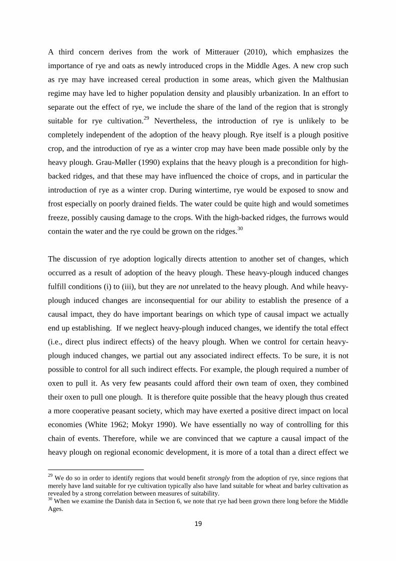
Table 1 presents the results for the non-flexible model. Turning first to urbanization as the
dependent variable, column 1 shows the results when the only controls are time and regional
fixed effects whereas column 2 includes all controls. Inspection of the table reveals that the
effect of having plough suitable area is positive and significant, both with and without control
variables. In columns 3 and 4 we check our results using population density as our measure
of economic development. In this case, the effect is also positive and significant.
In order to evaluate the economic size of impact of the heavy plough, we calculate regional
urbanization and population densities in a counterfactual setting where the plough never was
introduced. That is, we first use the urbanization and population densities from our last period
of observation and subtract the estimated effect of adopting the heavy plough:34
. We then aggregate over all regions
34
We use the estimated effects from the models in columns two and four of Table 1. In a few cases the
counterfactual population density or urbanization becomes negative. This happens when the estimated effect of
the heavy plough exceeds the actual level of development in AD 1300. In those cases we set the counterfactual
equal to zero. Still, using the negative counterfactual creates nearly identical results.

22
and calculate the average urbanization in a world without the heavy plough, which is found to
be 0.000305 cities per km2. This should be compared to the actual urbanization of 0.000321.
In AD 900, before the heavy plough became widespread, the urbanization rate had reached
0.000205. Hence, in the counterfactual setting the increase would have been 0.000100
compared to the actual increase of 0.000117; or, to put it differently, the increase would have
been only 85.7% of the actual increase. This means that the heavy plough explains 14.3 % of
the increase in urbanization from AD 900 to 1300 holding everything else constant.
Calculating the same for population density yields smaller but yet comparable results; the
heavy plough explains 7.7 % of the increase in population density over the same period. That
the heavy plough explains as much as one tenth of the increase in productivity observed in
the High Middle Ages is not unreasonable, keeping in mind that we are considering the total
effect of the plough in a purely agricultural economy.35
5.2 Flexible model
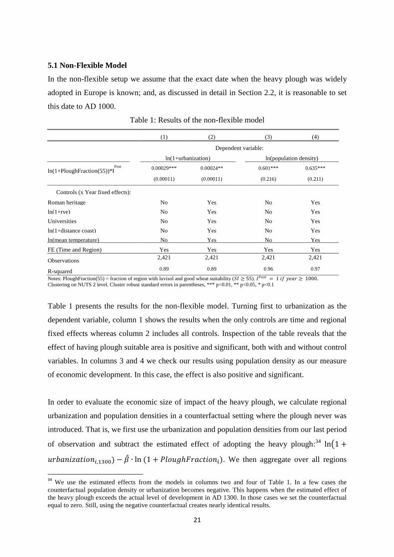
Turning to the flexible model, where the timing of the widespread diffusion of the plough is
assumed unknown, we report results in Table 2. The four columns correspond to the same
columns in Table 1. As is evident upon inspecting the table, as of AD 900 the plough’s effect
on urbanization increases and the precision of the estimated effect also rises, cf. columns 1
and 2. With respect to population density, we see the same increasing effect but with the
precision of the estimated effect rising even faster over time, cf. columns 3 and 4.
The picture that emerges is thus one showing that the heavy plough had a significant effect on
population density after AD 900, and that over time its impact became increasingly
important. This is fully consistent with the view that the plough started to spread across
Europe in earnest at the closing of the first millennium AD. In earlier centuries, before the
breakthrough of the heavy plough, there was no effect of having fertile, heavy clay soil.36
35
An alternative way to gauge the economic effect is to evaluate the marginal effects at mean values. For
urbanization, the formula is
. If we consider moving
from having no plough suitable land to having the mean share, we obtain (upon inserting values from Appendix
B and Table 1):
This means that the relative
increase is 0.0000224/0.000342 = 6.54%. Doing a similar calculation for population density gives a relative
increase of 0.6246/10.52863= 5.93%. 36
We note that the dummies for AD 600 and 700 are marginally significant at the 10 percent level when we
include our full set of controls in the urbanization model. This is likely to be a fluke. First, significance is absent
in the model without controls, and when we formally test whether any of these coefficients are significant by
means of a Bonferonni test (see Mittelhammer et al, 2000) which requires that the smallest p-value is less than
0.10/4, we fail to reject the hypothesis that at least one coefficient is significant. Further, the finding is non-
23
Hence the results based on the more demanding flexible model are consistent with those of
the non-flexible model.
Table 2: Results of the flexible model
(1) (2) (3) (4)
Dependent variable:
ln(1+Urbanization)
ln(Population density)
ln(1+PloughFraction(55)) *I
600
0.00006 0.00008* -0.129 -0.226
(0.00005) (0.00005) (0.151) (0.143)
ln(1+PloughFraction(55)) *I700
0.00008 0.00011* -0.134 -0.313**
(0.00006) (0.00006) (0.133) (0.121)
ln(1+PloughFraction(55)) *I800
0.00002 0.00000 0.076 -0.015
(0.00006) (0.00007) (0.102) (0.081)
ln(1+PloughFraction(55)) *I900
0.00011 0.00009 0.324** 0.338**
(0.00009) (0.00009) (0.154) (0.152)
ln(1+PloughFraction(55)) *I1000
0.00022* 0.00020 0.447** 0.527**
(0.00012) (0.00012) (0.210) (0.213)
ln(1+PloughFraction(55)) *I1100
0.00029** 0.00023* 0.499** 0.555***
(0.00013) (0.00013) (0.212) (0.208)
ln(1+PloughFraction(55))*I1200
0.00041*** 0.00038** 0.717*** 0.628***
(0.00015) (0.00016) (0.237) (0.233)
ln(1+PloughFraction(55))*I1300
0.00045*** 0.00035** 0.848*** 0.658**
(0.00017) (0.00017) (0.274) (0.264)
Controls (x Year fixed effects):
Roman Heritage No Yes No Yes
Rye No Yes No Yes
Universities No Yes No Yes
Distance Coast No Yes No Yes
Mean Temperature No Yes No Yes
FE (Time and Region) Yes Yes Yes Yes
Observations 2,421 2,421 2,421 2,421
R-squared 0.89 0.89 0.96 0.97
Notes: PloughFraction(55) = fraction of region with luvisol and good wheat suitability ( ). . Clustering on NUTS 2 level. Cluster robust standard errors in parentheses, *** p<0.01, ** p<0.05, * p<0.1
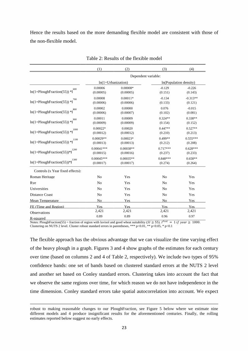
The flexible approach has the obvious advantage that we can visualize the time varying effect
of the heavy plough in a graph. Figures 3 and 4 show graphs of the estimates for each century
over time (based on columns 2 and 4 of Table 2, respectively). We include two types of 95%
confidence bands: one set of bands based on clustered standard errors at the NUTS 2 level
and another set based on Conley standard errors. Clustering takes into account the fact that
we observe the same regions over time, for which reason we do not have independence in the
time dimension. Conley standard errors take spatial autocorrelation into account. We expect
robust to making reasonable changes to our PloughFraction, see Figure 5 below where we estimate nine
different models and 4 produce insignificant results for the aforementioned centuries. Finally, the rolling
estimates reported below suggest no early effects.
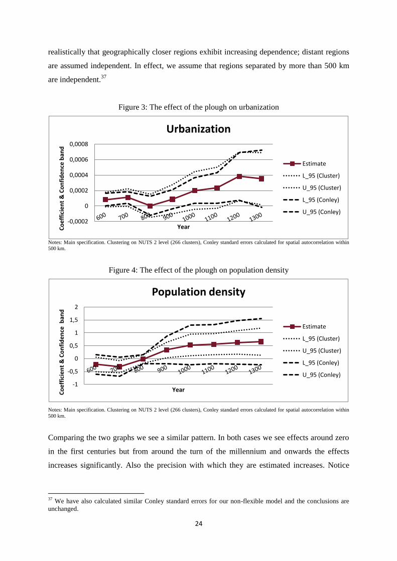
24
realistically that geographically closer regions exhibit increasing dependence; distant regions
are assumed independent. In effect, we assume that regions separated by more than 500 km
are independent.37
Figure 3: The effect of the plough on urbanization
Notes: Main specification. Clustering on NUTS 2 level (266 clusters), Conley standard errors calculated for spatial autocorrelation within
500 km.
Figure 4: The effect of the plough on population density
Notes: Main specification. Clustering on NUTS 2 level (266 clusters), Conley standard errors calculated for spatial autocorrelation within
500 km.
Comparing the two graphs we see a similar pattern. In both cases we see effects around zero
in the first centuries but from around the turn of the millennium and onwards the effects
increases significantly. Also the precision with which they are estimated increases. Notice
37
We have also calculated similar Conley standard errors for our non-flexible model and the conclusions are
unchanged.
-0,0002
0
0,0002
0,0004
0,0006
0,0008
Co
eff
icie
nt
& C
on
fid
en
ce b
and
Year
Urbanization
Estimate
L_95 (Cluster)
U_95 (Cluster)
L_95 (Conley)
U_95 (Conley)
-1
-0,5
0
0,5
1
1,5
2
Co
eff
icie
nt
& C
on
fid
en
ce b
and
Year
Population density
Estimate
L_95 (Cluster)
U_95 (Cluster)
L_95 (Conley)
U_95 (Conley)
25
that the effect on urbanization becomes significant approximately one to two centuries later,
which may indicate a lagged effect of population on urbanization.
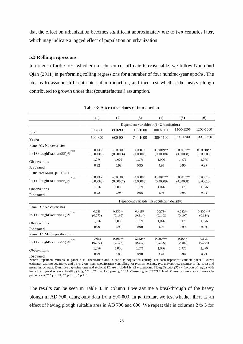
5.3 Rolling regressions
In order to further test whether our chosen cut-off date is reasonable, we follow Nunn and
Qian (2011) in performing rolling regressions for a number of four hundred-year epochs. The
idea is to assume different dates of introduction, and then test whether the heavy plough
contributed to growth under that (counterfactual) assumption.
Table 3: Alternative dates of introduction
(1) (2) (3) (4) (5) (6)
Dependent variable: ln(1+Urbanization)
Post: 700-800 800-900 900-1000 1000-1100 1100-1200 1200-1300
Years: 500-800 600-900 700-1000 800-1100 900-1200 1000-1300
Panel A1: No covariates
ln(1+PloughFraction(55))*IPost
0.00002 -0.00000 0.00012 0.00019** 0.00018** 0.00018**
(0.00005) (0.00006) (0.00008) (0.00008) (0.00008) (0.00009)
Observations 1,076 1,076 1,076 1,076 1,076 1,076
R-squared 0.92 0.93 0.95 0.95 0.95 0.95
Panel A2: Main specification
ln(1+PloughFraction(55))*IPost
0.00002 -0.00005 0.00008 0.00017** 0.00016** 0.00015
(0.00005) (0.00007) (0.00008) (0.00009) (0.00008) (0.00010)
Observations 1,076 1,076 1,076 1,076 1,076 1,076
R-squared 0.92 0.93 0.95 0.95 0.95 0.95
Dependent variable: ln(Population density)
Panel B1: No covariates
ln(1+PloughFraction(55))*IPost
0.035 0.332** 0.415* 0.273* 0.222** 0.309***
(0.073) (0.168) (0.214) (0.142) (0.107) (0.114)
Observations 1,076 1,076 1,076 1,076 1,076 1,076
R-squared 0.99 0.98 0.98 0.98 0.99 0.99
Panel B2: Main specification
ln(1+PloughFraction(55))*IPost
-0.051 0.405** 0.542** 0.380*** 0.164* 0.125
(0.073) (0.177) (0.217) (0.136) (0.089) (0.094)
Observations 1,076 1,076 1,076 1,076 1,076 1,076
R-squared 0.99 0.98 0.98 0.99 0.99 0.99
Notes: Dependent variable in panel A is urbanization and in panel B population density. For each dependent variable panel 1 shows estimates with no covariates and panel 2 our main specification controlling for Roman heritage, rye, universities, distance to the coast and
mean temperature. Dummies capturing time and regional FE are included in all estimations. PloughFraction(55) = fraction of region with
luvisol and good wheat suitability ( ). . Clustering on NUTS 2 level. Cluster robust standard errors in parentheses, *** p<0.01, ** p<0.05, * p<0.1
The results can be seen in Table 3. In column 1 we assume a breakthrough of the heavy
plough in AD 700, using only data from 500-800. In particular, we test whether there is an
effect of having plough suitable area in AD 700 and 800. We repeat this in columns 2 to 6 for

26
the periods 600-900, 700-1000, 800-1100, 900-1200, and 1000-1300. A result consistent with
the cut-off date being AD 1000 would be insignificance for the cases that do not include AD
1000 in the post-adoption period. For the later rolling periods, where the heavy plough
presumably was already in widespread use, post- and pre-adoption periods will in effect both
have been treated.
By and large, the rolling regressions reveal an increasing effect over time. In panel A1 and
A2, where urbanization is used, the point estimate of the effect of the heavy plough increases
significantly when both post centuries contains 1000 AD and 1100 AD. This is not surprising
given that this is the first specification where both pre-centuries are in the expected untreated
range and both post-centuries are in the expected treatment range. In the third specification
the picture is largely the same unless that the effect comes two centuries earlier. However, in
Panel B2 the excess effect is highest around the turn of the millennium; subsequently, the size
and significance of the effect diminishes. This could indicate that it became harder to keep
increasing output even more as the plough was already widespread and the best soils was
already being cultivated. It is also consistent with the view that the effect on population
density started earlier than the effect on urbanization. Again this could be a result of a lagged
effect of population density on urbanization. Of course, we should beware not to interpret too
much into this, as we cannot reject that null hypothesis that all statistically significant point
estimates in Panel B are equal.
5.4 Robustness
So far we have found strong evidence that the heavy plough had a sizeable and increasing
impact on regional economic development as of the closing of the first millennium. In this
section we report on the sensitivity of our results with respect to permutations of the main
independent variable. First, in Section 5.4.1, we check whether the results are robust to
alternative measures of plough suitable land. Second, in Section 5.4.2, we conduct a placebo
type experiment.
5.4.1 Alternative measures of heavy plough suitable land
So far we have worked with a measure of plough suitable land that relies on luvisol and good
conditions for growing wheat.38
This choice of soil, suitability level and crop may be
questioned. Consequently, we first look into the consequences for our results when using 38
Specifically, we have worked with PloughFraction(55), cf. footnote 24.

27
alternative crops, such as barley and rye, as well as alternative suitability levels for growing
the crops. Second, we add another soil type, gleysol, in order to broaden our measure of soils
that may benefit from the heavy plough.
Alternative crops and suitability levels
The results for the non-flexible model when using alternative crops and suitability levels are
shown in Table 4. Our baseline result is the one in the middle of the first column. We see that
the results are highly stable to alternative plough positive crops. The change in suitability
level and crop slightly changes the magnitude and the significance of the results. The size of
the effect increases as the suitability increases. This is an intuitive result: more suitable
conditions would make it even more beneficial to be able to cultivate the land.
Table 4: Non-flexible estimates for different crops and suitability levels
Crop
Wheat Rye Barley
Su
itab
ilit
y a
t le
ast
PloughFraction (40)
0.00025** 0.00025** 0.00023**
(0.00011) (0.00010) (0.00011)
PloughFraction (55) 0.00024** 0.00026** 0.00026**
(0.00011) (0.00011) (0.00011)
PloughFraction (70)
0.00030** 0.00028* 0.00033**
(0.00014) (0.00016) (0.00016)
Notes: Dependent variable is urbanization. Main specification controlling for
Roman heritage, rye, universities, distance to the coast and mean temperature.
Dummies capturing time and regional FE are included. PloughFraction(SI) =
fraction of region with luvisol and crop suitability according to the table. Clustering on NUTS 2 level. Cluster robust standard errors in parentheses, *** p<0.01, **
p<0.05, * p<0.1
Figure 5 investigates exactly the same issue for the flexible model. So we estimate the model
using different alternative crops and suitability levels for growing the alternative crop. The
graphs reveal a similar picture across crops and suitability level. Again the effect and
increases with the suitability level for the same reasons as mentioned above. At the same time
precision decreases, probably due to the fact that areas that in reality are suitable are included
as unsuitable. Given the results in table 4 and figure 5 we conclude that our results are stable
to the use of alternative measures of suitability39
. Next we turn the sensitivity of our choice of
soil type.
39
Carrying out the same robustness tests for population density using flexible as well as non-flexible models
leads to the same conclusion. Results are available upon request.

28
Figure 5: Flexible estimates for different crops and suitability levels
Wheat Rye Barley
Plo
ughF
ract
ion
(40)
Plo
ughF
ract
ion (
55)
Plo
ughF
ract
ion (
70)
Notes: Dependent variable is urbanization. Main specification controlling for Roman heritage, rye, universities, distance to the coast, and
mean temperature. Dummies capturing time and regional FE are included. PloughFraction(SI) = fraction of region with luvisol and crop suitability according to the table. Clustering on NUTS 2 level.
Measure including gleysol.
As we discussed above, luvisol fits well with the soils that historians point to as being
suitable for the heavy plough. But there might be other soils that would gain from the heavy
plough. Gleysol, which is a wetland soil (FAO, 2006), is described by Edwards (1990, p. 50)
as poorly drained soil for the case of the Ireland. Since one of the advantages of the heavy
plough was its ability to assist drainage we add this soil to our plough measure, both in order
to test the sensitivity of our choice of luvisol but also to test for a potential impact in these
-0,0002
0
0,0002
0,0004
0,0006
0,0008
-0,0002
0
0,0002
0,0004
0,0006
0,0008
-0,0002
0
0,0002
0,0004
0,0006
0,0008
-0,0002
0
0,0002
0,0004
0,0006
0,0008
-0,0002
0
0,0002
0,0004
0,0006
0,0008
-0,0002
0
0,0002
0,0004
0,0006
0,0008
-0,0004
-0,0002
0
0,0002
0,0004
0,0006
0,0008
0,001
-0,0004
-0,0002
0
0,0002
0,0004
0,0006
0,0008
0,001
0,0012
-0,0005
0
0,0005
0,001
0,0015

29
areas. Figures 6 and 7 show that the overall picture is the same and, in fact, including gleysol
increases the effect especially so in the period around and after the breakthrough of the heavy
plough. Whether the extra gain in these areas stems from the heavy plough is difficult to say;
they could have gained a lot from improved drainage using the heavy plough but perhaps also
other effects are in operation given the size of the effect. At any rate, nothing changes
qualitatively.
Figure 6: Comparison of urbanization estimates including gleysol
Notes: Dependent variable is urbanization. Main specification. PloughFraction(55) = fraction of region with luvisol or gleysol and good
wheat suitability ( ). Each graph shows the point estimates for each century.
Figure 7: Comparison of population density estimates including gleysol
Notes: Dependent variable is population density. Main specification. PloughFraction(55) = fraction of region with luvisol or gleysol and
good wheat suitability ( ). Each graph shows the point estimates for each century.
All plough positive crops
We also try to include all three plough positive crops simultaneously in our plough measure;
that is, the suitability for one of the crops wheat, rye or barley should be at least “good”
0
0,0001
0,0002
0,0003
0,0004
0,0005
0,0006
Co
eff
icie
nt
Year
Gleysol test, urbanization
Main specification
Including gleysol
-0,5
0
0,5
1
Co
eff
icie
nt
Year
Gleysol test, population density
Main specification
Including gleysol
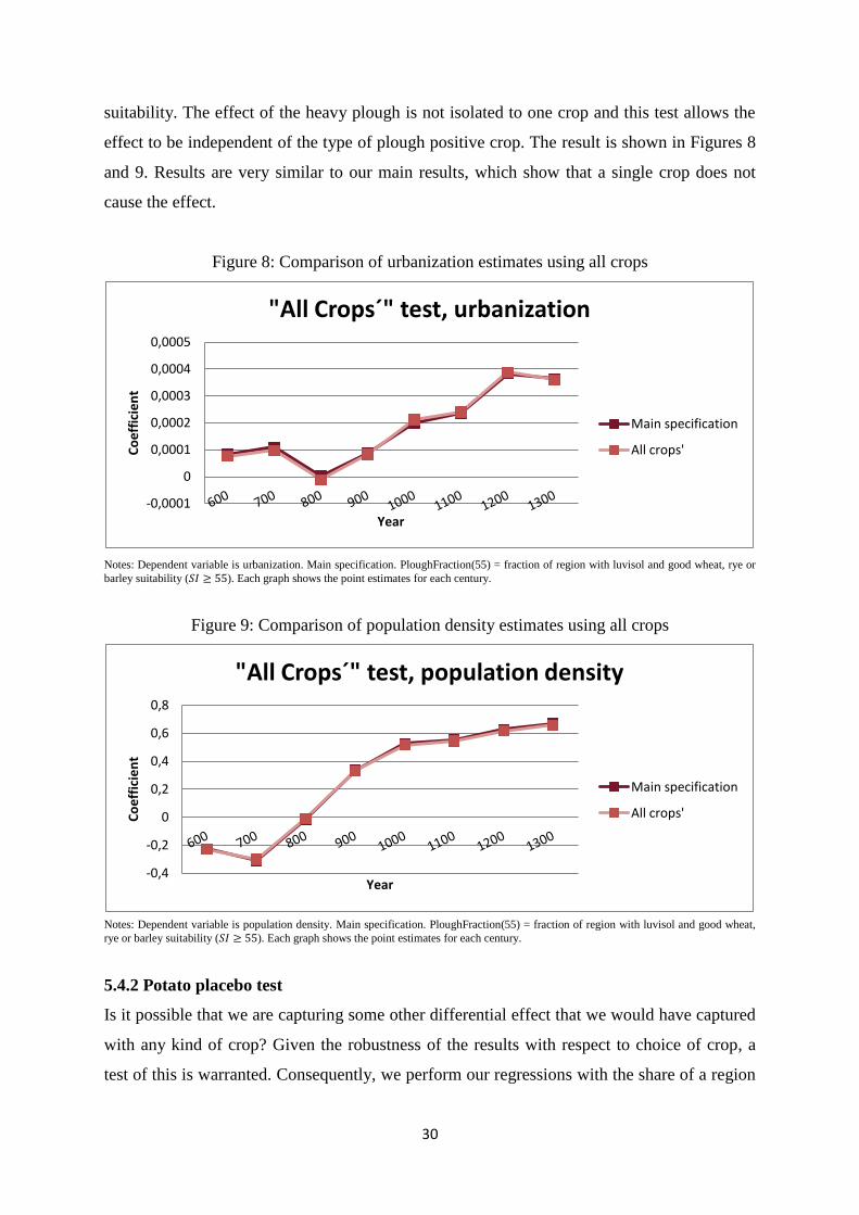
30
suitability. The effect of the heavy plough is not isolated to one crop and this test allows the
effect to be independent of the type of plough positive crop. The result is shown in Figures 8
and 9. Results are very similar to our main results, which show that a single crop does not
cause the effect.
Figure 8: Comparison of urbanization estimates using all crops
Notes: Dependent variable is urbanization. Main specification. PloughFraction(55) = fraction of region with luvisol and good wheat, rye or
barley suitability ( ). Each graph shows the point estimates for each century.
Figure 9: Comparison of population density estimates using all crops
Notes: Dependent variable is population density. Main specification. PloughFraction(55) = fraction of region with luvisol and good wheat,
rye or barley suitability ( ). Each graph shows the point estimates for each century.
5.4.2 Potato placebo test
Is it possible that we are capturing some other differential effect that we would have captured
with any kind of crop? Given the robustness of the results with respect to choice of crop, a
test of this is warranted. Consequently, we perform our regressions with the share of a region
-0,0001
0
0,0001
0,0002
0,0003
0,0004
0,0005
Co
eff
icie
nt
Year
"All Crops´" test, urbanization
Main specification
All crops'
-0,4
-0,2
0
0,2
0,4
0,6
0,8
Co
eff
icie
nt
Year
"All Crops´" test, population density
Main specification
All crops'

31
with good suitability for growing potatoes as our main independent variable. This is a
placebo-type experiment: We know that the potato strongly influenced urbanization and
population density in potato suitable areas after 1700 (Nunn and Qian 2011). However, as the
potato was unknown to Europeans before the discovery of the Americas, we should not see
any effect of potato suitable soil on population density and urbanization during our
observation window, 500-1300. Moreover, potatoes can successfully be grown on many types
of soils (Kopsell 2000), including sandy soils on which we know that the heavy plough is not
beneficial. Any such effect would imply that we are capturing a more general trend, and it
would seriously undermine our identification strategy. The results of the non-flexible model
are shown in Table 5, while Figures 10 and 11 show the flexible estimates with respectively
urbanization and population density as dependent variables.
Table 5: Placebo test
Notes: Main specification controlling for Roman heritage, rye, universities, distance to the coast and
mean temperature. Clustering on NUTS 2 level. Dummies capturing time and regional FE are included.
PotatoFraction(55) = fraction of region with good potato suitability ( ). PloughFraction(55) =
fraction of region with luvisol and good wheat suitability ( ). . Cluster
robust standard errors in parentheses, *** p<0.01, ** p<0.05, * p<0.1
Figure 10: Comparison of urbanization estimates using potato suitability
-0,0004
-0,0002
0
0,0002
0,0004
0,0006
0,0008
Co
eff
icie
nt
& C
on
fid
en
ce b
and
Year
Placebo test, urbanization
Potato
L_95
U_95
Main
L_95 (Cluster)
U_95 (Cluster)
(1) (2) (3) (4)
Dependent variable
ln(1+Urbanization) ln(Population density)
ln(1+PotatoFraction(55))*IPost
0.00008 -0.00534
(0.00010) (0.17300)
ln(1+PloughFraction(55))*IPost
0.00024** 0.638***
(0.00011) (0.21)
Observations 2,421 2,421 2,421 2,421
R-squared 0.89 0.89 0.97 0.97

32
Notes: Dependent variable: urbanization. Controlling for Roman heritage, rye, universities, distance to the coast and mean temperature.
Clustering on NUTS 2 level. Dummies capturing time and regional FE are included.
Figure 11: Comparison of population estimates using potato suitability
Notes: Dependent variable: population density. Controlling for Roman heritage, rye, universities, distance to the coast, and mean temperature. Clustering on NUTS 2 level. Dummies capturing time and regional FE are included.
Using potato suitability alters the results substantially. In the non-flexible as well as in the
flexible model the magnitude of the estimates decreases substantially and precision is
reduced, rendering estimates insignificant. In fact, for urbanization as well as population
density the effect completely vanishes. Overall, these results substantiate that the effect which
we attribute to the heavy plough is not just a general effect that any crop would give rise to;
and, in particular, not a crop that would turn out to be very important later in history.
6. Test on Danish regional data
A concern regarding our measures of economic development and our Ploughfraction measure
is that they are likely to be measured with substantial error. If the measurement error is
unsystematic, it only works against our alternative hypothesis in the sense of reducing the
precision of point estimates. If the measurement error is systematic, the consequences may be
less benign. To deal with this concern, we have constructed alternative and more precise
measures for both clay soil and urbanization for 25 Danish historical counties.40
In addition to
the advantage of more precise measures, a second advantage is that Denmark contains much
regional variation in terms of the presence of clay soils, which makes it an interesting case for
testing White’s hypothesis. A third advantage is that we can study the effects at a more local
40
We use the counties to capture much better the variation within Denmark. With NUTS regions, we only have
5 large regions and do not capture regional heterogeneities to the same extent. Further estimating with only 5
regions would give a very small dataset.
-1
-0,5
0
0,5
1
1,5
Co
eff
icie
nt
& C
on
fid
en
ce b
and
Year
Placebo test, population density
Potato
L_95
U_95
Main
L_95 (Cluster)
U_95 (Cluster)

33
level since we now use smaller geographical units, both in terms of historical counties rather
than larger present regions as well as towns rather than cities. Finally, the Danish case allows
us to shed some light on the plausibility of our maintained assumptions. For instance, we
have assumed that soil maps from the late 20th
century capture the location of medieval clay
soils well, as they formed during the ice age as noted above. The Danish data allow us to
show that the share of clay soil based on late 20th
century map correlates positively and
significantly with the share of clay soil calculated on the basis of an early 20th
century
geological map for Denmark taken from Harder and Ussing (1913), see Appendix D. We also
demonstrate in Appendix D that our modern measure of suitability for growing barley
correlates positively and significantly with a measure of peasant payments in terms of barley
to landlords from the early 1660s as well as crop yields in the 1830s. This supports that soil
suitability today captures that of the past, which is another maintained assumption. Before we
turn to the results, we briefly discuss 1) the timing of the breakthrough of the heavy plough in
Denmark, 2) the construction of the new measures, and 3) the included control variables.
Timing of breakthrough
As in the analysis of the European case, we need to determine the timing of the breakthrough
in order to estimate the nonflexible model. Therefore, we briefly review the existing Danish
evidence. As for Europe in general, most historians stress that the breakthrough took place
around AD 1000 or after. Grau-Møller (1990) notes that the earliest dating of high backed
ridges is from around AD 1000, but that the more certain dating is for the 1100s. Poulsen
(1997, p.116) is in line with this and summarizes the diffusion process as follows: “Probably
around 900 to 1100, then the mouldboard plough was introduced into Denmark, gradually
diffusing from southern areas.” Moreover, and as noted above, the word for plough in Old
Norse does not appear before AD 1000. Jensen (2010, p. 202) argues that the breakthrough
happened in the middle of the 1100s. He bases this on the presence of high backed ridges, as
do other authors, but also stresses that heavy ploughs are mentioned in Danish medieval
provincial laws from the second half of the 1100s and early 1200s.41
Larsen (2011, p. 124)
argues that the earliest evidence of introduction is from AD 200-400 based on two cases from
Western Jutland, though both these two cases remain controversial.42
He concludes that the
41
Porsmose (1988, p.285) mentions that the Danish word for plough (plov) was introduced into Danish history
as the man who killed King Erik Emune in 1137 was named black plough. 42
For the first case, Larsen (2011, p.96) grants that the dating is problematic, and whether the ridges are proper
high backed ridges has been questioned by other experts (Grau-Møller, personal communication). For the
34
introduction in Western Jutland should be dated to this time (Larsen 2011, p. 124). In the rest
of Jutland, the plough may have been used in the early medieval period. While this evidence
is suggestive of an early adoption in some places, it does not provide solid evidence for the
breakthrough. Given that we used AD 1000 in the European case, and given that some
evidence for this year is present, we stick to this timing in the nonflexible model, but we do
investigate the timing in the flexible model in order to evaluate this choice.
Empirical model and data
We implement an empirical specification along the lines equations (1) and (2), but modify the
measures accordingly. The cross-sectional dimension is now the 25 Danish historical
counties.
As our new urbanization measure, we construct the town density for each county based on
Jensen’s (2010) dating of the approximate establishment of Danish medieval towns.43
He
used among other things information on when the town had main streets, a town centre with a
market square, and a town church to give an approximate earliest date of when the town was
established in the sense that it included these elements (Jensen 2010, pp.77-79). Jensen
provides data for the timing of the establishment of towns for every 25 years, and from this
we obtain towns per square kilometer every 25 years from AD 675 to 1300. This measure is
analogous to our city density measure in the European sample.
We also construct a new PloughFraction measure. We have digitized the soil map from
Frandsen (1988), which gives the locations of clay soils in Denmark (see Figure 12).44
Jensen
(2010) used this map to pinpoint the location and types of soil that would benefit from heavy
plough. This measure is more precise than the luvisol based measure used above and, in
contrast to the luvisol measure, captures all clay soils. The luvisol based measure is highly
correlated with the new measure,45
but some of the moraine clay soils on Zealand in East
Denmark are not captured by the luvisol measure. We also note that the most of the
remaining Danish soils are classified as sandy soils. PloughFraction is constructed as the
second case, Larsen (pp.110-112) notes that there is scholarly disagreement on this, as some scholars reject that
the furrows could have been produced by a heavy plough. 43
See table E3 in appendix E for a complete list of the Danish towns and cities. 44
We use the three categories (clay soils, sandy, clay soils and clayey, sandy soils) as suggested by Jensen
(2010) to measure clay soils. We also add clay soils and heavy clay soils from Frandsen’s original map that
Jensen (2010) left out, though there is relatively little soil of these types in Denmark. 45
The correlation coefficient is 0.70 and strongly significant.
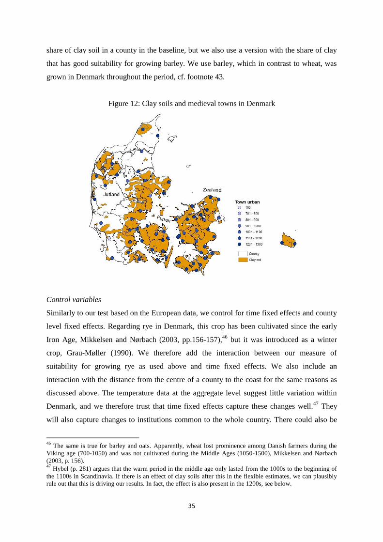
35
share of clay soil in a county in the baseline, but we also use a version with the share of clay
that has good suitability for growing barley. We use barley, which in contrast to wheat, was
grown in Denmark throughout the period, cf. footnote 43.
Figure 12: Clay soils and medieval towns in Denmark
Control variables
Similarly to our test based on the European data, we control for time fixed effects and county
level fixed effects. Regarding rye in Denmark, this crop has been cultivated since the early
Iron Age, Mikkelsen and Nørbach (2003, pp.156-157),46
but it was introduced as a winter
crop, Grau-Møller (1990). We therefore add the interaction between our measure of
suitability for growing rye as used above and time fixed effects. We also include an
interaction with the distance from the centre of a county to the coast for the same reasons as
discussed above. The temperature data at the aggregate level suggest little variation within
Denmark, and we therefore trust that time fixed effects capture these changes well.47
They
will also capture changes to institutions common to the whole country. There could also be
46
The same is true for barley and oats. Apparently, wheat lost prominence among Danish farmers during the
Viking age (700-1050) and was not cultivated during the Middle Ages (1050-1500), Mikkelsen and Nørbach
(2003, p. 156). 47 Hybel (p. 281) argues that the warm period in the middle age only lasted from the 1000s to the beginning of
the 1100s in Scandinavia. If there is an effect of clay soils after this in the flexible estimates, we can plausibly
rule out that this is driving our results. In fact, the effect is also present in the 1200s, see below.
36
regional effects of institutional change. From the late 900s, Denmark was ruled by one king,
and this may have influenced regional development. Jutland (the peninsular which shares a
border with Germany) had proved difficult to defend, and it has been argued that Zealand
(see figure 12) was more easily defended. This may have led to a change in gravitational
centre towards the eastern part of Zealand. In fact, some eastern towns were founded by the
second Danish king around AD 1000 (Sawyer 2002, pp. 355-56). We address this by testing
whether our results still hold within Jutland. The test within Jutland also helps address that
different regions had different provincial laws. Jutland’s provincial law (known as “Jyske
lov”)—a law that among other things regulated how the farmland was distributed within a
village and that tried to incentivize agricultural expansion—is from AD 1241(Porsmose
1988). Since this law was the same across Jutland, we capture its effects by time fixed
effects.
Results
In order to save space, we report mainly nonflexible estimations, cf. Table 6. We calculate
both standard errors corrected for clustering at the county level as reported in Table 6 and
Conley standard errors that correct for spatial autocorrelation. We have allowed counties
further apart than 200 km to be independent. Spatial autocorrelation does not affect our
results, as we obtain similar results regardless of type of the standard errors.
Column 1 reports the baseline measure when we only control for county and time fixed
effects. Column 2 reports results when using only clay soil with good suitability for growing
barley, as in the European analysis. Both regressions show a positive and significant effect of
clay soils from AD 1000. Using the quality adjusted measure has little impact on our results;
in fact, it only strengthens them. It turns out that the fertile soils (in terms of plough friendly
crops) largely coincide with the clay soils of Denmark, and unsurprisingly we therefore find
that there is little effect of making this correction. In column 3, where we add extra
covariates, we find the regression coefficient hardly changes.
We mentioned above that the move to rule by one king led to a shift towards the island of
Zealand for reasons of national defense. Given that the shift was away from Jutland, we can
test whether the shift towards Zealand explains our result by testing solely on Juttish
counties. Doing this shows that the effect still emerges, though with a smaller but significant
coefficient. This suggests that the effect of clay soil areas is not merely due to the move to

37
rule by one king, see column 4. The inclusion of fixed effects captures potential regional
institutional shocks. In columns 5 and 6, we use the luvisol measure both unadjusted and
adjusted for quality. While we find similar results, the coefficients are smaller and less
precisely estimated. We already mentioned above that some clay soils are not classified as
luvisol. This is particular true for the county of Sorø, and if we drop this observation results
become stronger. Given that the Danish case has relevance for Northern Europe in general, it
suggests that we may miss some clay soil in the luvisol based measure above.48
Still, the fact
that we obtain similar, albeit weaker, results suggests that this choice is a reasonable starting
point. Finally, Jensen (2010) includes clayey sandy soils among the soils that would benefit
from the heavy plough. This choice may be questioned since this soil is not defined as clay
soil. On the other hand, the sandy clay soils often coincide with areas that the older map
mentioned above classifies as moraine clay.49
Still, we investigate the importance of this soil
type by excluding it from our measure in column 7, and we reach a similar conclusion as in
the baseline measure.
Table 6: The results for the Danish dataset
(1) (2) (3) (4) (5) (6) (7)
Dependent variable: ln(1+Urbanization)
Clay
Clay with
good barley
suitability
Clay with all
covariates
Clay for
subsample
Jutland Luvisol
Luvisol with
good barley
suitability
Clay without
clayey sand
soil
ln(1+PloughFraction(55)) *IPost
0.00169*** 0.00164*** 0.00168*** 0.00063* 0.00097* 0.00105* 0.00163*** (0.00031) (0.00030) (0.00049) (0.00031) (0.00050) (0.00054) (0.00024)
Distance Coast No No Yes Yes No No No
ln(1+rye) No No Yes Yes No No No
FE (Time and county) Yes Yes Yes Yes Yes Yes Yes
Observations 650 650 650 364 650 650 650
R-squared 0.71 0.71 0.75 0.82 0.68 0.68 0.72
Notes: PloughFraction = fraction of county with clay (columns 1, 3, and 4), = fraction of county with clay and good rye suitability (column
2), = fraction of county with luvisol (column 5), = fraction of county with luvisol and good wheat suitability (column 6), = fraction of region
with clay but not clayey sand (column 7). Column 6 only includes counties in Jutland. Controls interacted with time fixed effects. Clustering on county level. Cluster robust standard errors in parentheses, *** p<0.01, ** p<0.05, * p<0.1
48 The Sorø area is classified as mainly cambisol according to the European soil database. This suggests that
some cambisol is clay soil, and may be better classified as clay soils. We have investigated the effect of
including fertile cambisol in our PloughFraction measure. Effects become stronger and more significant,
increasing to the 1 percent level for urbanization. Thus, these results are in line with what we find for Denmark. 49
We have re-estimated the models in Table 6 using a clay soil measure based on the older map and obtain
similar results. We prefer the modern map since it covers all counties. In the period 1864-1920, the three
counties near the
Danish-German border were under German control.

38
When we evaluate the effect of the heavy plough in a counterfactual setting similar to the one
for the European case, we find that 70.6 % of urbanization can be attributed to the heavy
plough based on model in column 1 of Table 6. This is a large effect, but hardly surprising
given the amount of clay soil in Denmark and our use of towns rather than cities.
Figure 13: The effect of the plough on urbanization in Denmark
Turning finally to the flexible regressions, we obtain similar results. We show one
representative example in Figure 13, which controls for covariates. The effect of clay soils
increase over time and becomes significant as of AD 1175, with point estimates increasing
from this time onwards. Results are similar for the other models. This suggests that a cut-off
after AD 1150 is reasonable; and if we use this cut-off in our non-flexible model, we obtain
larger estimates. We also note that the timing of the effect is later than both the warm
medieval period in Denmark and the shift to rule by one king. In sum, the Danish case
provides strong evidence that the breakthrough of the heavy plough mattered for
development.
7. Conclusion
This paper provides the first rigorous empirical examination of the “heavy plough
hypothesis”, proposed by White (1962). The hypothesis holds that the heavy plough played
an important role for population growth and urbanization in the Middle Ages. The results
emerging from our analysis of two datasets strongly corroborate the hypothesis. Based on the
European data, we find that the heavy plough accounts for one tenth of the increase in
urbanization and population density experienced in the High Middle Age. Our paper
-0,002
0
0,002
0,004
0,006
0,008
Co
eff
icie
nt
& C
on
fid
en
ce b
and
s
Year
PloughArea x Year Indicator
Estimate
L_95 (Cluster)
U_95 (Cluster)
L95 (Conley)
U95 (Conley)

39
therefore importantly complements the qualitative accounts found in the historiographical
literature on medieval technology.
This paper also speaks to the modern literature on the deep determinants of economic
development. Specifically, we analyze an important example of the sophisticated geography
hypothesis: Clay soils conferred no advantages prior to the introduction of the heavy plough;
once the heavy plough arrived, access to the fertile clay soils provided advantages in terms of
productivity, access to new and fertile land, etc.
Our empirical analysis naturally contains some weaknesses. First, since we estimate the total
effect of the heavy plough, the paper is unable to add to the debate on the relative importance
of institutions versus geography in economic development (see Acemoglu et al. 2005a).
Second, identification of a causal impact rests on our ability to control for all other changes
unrelated to the heavy plough that occurred around the time of plough adoption in Europe,
and at the same time both correlate with plough suitability and affect urbanization and/or
population density. Third, we have to assume the geology of the period from AD 500 to 1300
is similar to that of later periods. For the Danish case, we can show that present day soil
suitability matches that of the 17th
and 19th
centuries, but for the rest of Europe we have to
rely on modern geology. We leave attempts to improve the analysis along the said
dimensions for future research.

40
8. References
Acemoglu, D., Johnson, S. and Robinson J., 2001. “The Colonial Origins of Comparative
Development: An Empirical Investigation,” American Economic Review, 91, 1369-1401
Acemoglu, D., Johnson, S. and Robinson J., 2005a. “Institutions as a Fundamental Cause of
Economic Growth.” In Aghion, P. and S. Durlauf (eds). “Handbook of Economic Growth”,
Amsterdam, Holland, North-Holland.
Acemoglu, D., Johnson, S. and Robinson J., 2005b. “The Rise of Europe: Atlantic Trade,
Institutional Change and Economic Growth,” American Economic Review, 95 (3), 546-579.
Alexandrovskiy, A., 2000. ”Holocene development of soils in response to environmental
changes: the Novosvobodnaya archaeological site, North Caucasus,” Catena 41, 237–248
Andersen, S. H and Nielsen P. O., 1982. ”Jæger og bonde i stenalderen,” Copenhagen:
Forlaget Sesam A/S.
Ashraf, Q. and Galor, O., 2011. “Dynamics and Stagnation in the Malthusian Epoch,”
American Economic Review, 101, 2003-2041
Astill, G., 1997. “An archaeological Approach to the Development of Agricultural
Technologies in Medieval England.” In Langdon, J., Astill, G., and Myrdal, J. (eds).
‘Medieval Farming and Technology’, Leiden, Netherlands: Brill.
Bairoch, P., 1988. “Cities and Economic Development: From the Dawn of History to the
Present,” Chicago, IL: University of Chicago Press
Bairoch, P., Batou, J. and Chevre, P., 1988. “The population of European Cities from 800 to
1850,” Centre of Internatonal Economic History, Geneva University, Geneva
Bartlett, R., 1993. “The Making of Europe,” Allen Lane, Great Britain.
Baten, J. Van Zanden, J.L., 2008. Book production and the onset of modern economic
growth. Journal of Economic Growth, 13, 217–235
Beresford, M. W., 1967. ”New towns of the Middle Ages: town plantation in England,
Wales, and Gascony,” Lutterworth Press London
Bloch, M., 1966. “French Rural History,” Routledge & Kegan Paul Limited.
Broadberry, S., Leuwen, B. Van Zanden, J.L., 2012. Reversals of fortune: Holland, Britain
and the rise of the North Sea Area, 1270-1870. Paper presented at Hi-Pod conference in
Brussels.
Comet, G., 1997. “Technology and Agricultural Expansion in the Middle Ages: The Example
of France North of the Loire.” In Langdon, J., Astill, G., and Myrdal, J. (eds). ‘Medieval
Farming and Technology’, Leiden, Netherlands: Brill.
41
Denevan, W. M., 1992. “The pristine myth: The landscape of the Americas in 1492,” Annals
– Association of American Geographers 82, 369–385.
de Vries, J., 1976. “The Economy of Europe in an Age of Crisis, 1600-1750,” Cambridge,
UK: Cambridge University Press
Duby, G., 1968. “Rural economy and life in the medieval west,” United Kingdom: Edward
Arnold Ltd.
Edwards, N., 1990. “The Archaeology of Early Medieval Ireland,” London, UK: B.T.
Basford Limited
European Soil Database, 2006: http://eusoils.jrc.ec.europa.eu/esdb_archive/ESDB/Index.htm
FAO, 2006. World Reference Base for Soil Resources, 2006: A Framework for International
classification, correlation and communication.
Felgenhauer-Schmidt, S., 1993. ”Die sachkultur des mittelalters im lichte der archäologischen
funde,” Frankfurt am Main, Germany: Peter Lang GmbH
Fowler, P., 2002. “Farming in the first millennium AD, “ Cambridge, UK: Cambridge
University Press.
Frandsen, K.E., (1988). 1536-ca. 1720 in Bjørn, C. (eds.) Det danske landbrugshistorie, 1536-
1810.
Fussell, G.E., 1966. “Ploughs and Ploughing before 1800,” Agricultural History, 40 (3), 177-
186
Goldewijk, K. Klein, A. Beusen, and P. Janssen (2010). “Long term dynamic modeling of
global population and built-up area in a spatially explicit way,” HYDE 3.1, The Holocene 20
(4), 565-573.
Goldewijk, K. Klein, Beusen, A., van Drecht, G., de Vos, M., 2011. ”The HYDE 3.1
spatially explicit database of human-induced global land-use change over the past 12,000
years,” Global Ecology and Biogeography, 20, 73–86
Grau-Møller, P., 1990. “Højryggede agre – forskning og bevaring,” Bol og By, 90-118.
Grau-Møller, P., 1995. ”Højryggede agre i fynske skove,” Fortid og Nutid, 303-323.
Guiot, J., Corona, C. and ESCARSEL members, 2010. “Growing Season Temperatures in
Europe and Climate Forcings Over the Past 1400 Years,” PLoS ONE, 5 (4)
Guul-Simonsen, F. Heide Jørgensen, M,, Have, H., Håkansson, I., 2002. ”Studies of plough
design and ploughing relevant to conditions in Northern Europe,” Acta Agricultural
Scandinavia, Section B, Soil and Plant Science 52, 57-77.
42
Hardt, N., 2003. ”Jernalderens og vikingetidens landbrug”. In P. Ethelberg, N. Hardt, B.
Poulsen, A.B. Sørensen, 2003. ”Det sønderjyske landbrugs historie,”. Haderslev, Denmark:
Haderslev Museum.
Heaton, H., 1963. ”Economic History of Europe,” Harper & Row, Ltd, London
Harder, P. and Ussing, N.V.. (1913). Danmarks geologi i almenfattelig omrids. Danmarks
geologiske undersøgelse 3, 2. Copenhagen, Denmark: Andelsbogtrykkeriet i Odense.
Henning, J., 1987. “Südosteuropa zwischen Antike und Mittelalter,” Akademie verlag Berlin.
Hilton, R., 1963. Technical Determinism: The Stirrup and the Plough. Past & Present, 24,.
90-100.
Hodgett, G., 1972. “A social and economic history of medieval Europe,” London, UK:
Methuen & Co. Ltd.
Hybel, N., 2002. Klima og hungersnød i middelalderen. Historisk Tidsskrift 102:2, 265-280
Hybel, N and Poulsen, B., 2007. “The Danish Resources c. 1000-1550: Growth and
Recession,” Brill
Jacobsen, N.K. (1984). Soil map of Denmark according to the FAO-UNESCO legend (p1.1).
Geografisk tidsskrift 84.
Jensen, J. E., 2010 “Gensidig afhængighed,” Syddansk universitetsforlag.
Jope, E.M., 1956. ”Agricultural implements.” In Charles Singer, E.J. Holmyard, A.R. Hall,,
Trevor I. Williams (eds). “A history of technology, Vol. 2: Mediterranean civilizations and
the Middle Ages,” Oxford, UK: Clarendon Press.
Kishlansky, M., Geary, P., O’Brien, P., 2010. “Civilization in the West,” Pearson,
International Edition
Kopsell, D., 2000. Growing potatoes. Fact sheet downloaded from university of New
Hampshire at:
http://extension.unh.edu/resources/representation/Resource000606_Rep628.pdf
Landes, D. S., 1998. “The wealth and poverty of nations: why some countries are so rich and
some so poor,” New York: WW Norton
Langdon, J., Astill, G., and Myrdal, J., 1997. “Introduction.” In Langdon, J., Astill, G., and
Myrdal, J. (eds). “Medieval Farming and Technology,” Leiden, Netherlands: Brill.
Langer, William L., 1972. “An encyclopedia of world history,” 5th Ed. Boston: Houghton
Mifflin Co.
Larsen, L.A., 2011. ”Mulfjælsploven i Danmark,” Århus, Denmark: Moesgård.

43
Lerche, G., 1994. “Ploughing implements and tillage practices in Denmark from the Viking
period to about 1800,” Herning, Denmark: Poul Christensen.
Livi-Bacci, M., 2007. “A Concise History of World Population,” Fourth edition. Oxford:
Blackwell Publishing
Louwagie, G., Gay, S. H., Burrell, A., 2009. “Addressing Soil Degradation in EU
Agriculture: Relevant Processes, Practices and Policies,” JRC Scientific and Technical
Reports
Maddison, A., 2001. “The World Economy: A Millennial Perspective,” Paris: OECD
Manning, W.H., 1964. “The plough in roman Britain,” The Journal of Roman Studies, 54,
Parts 1 and 2 (1964), 54-65
McEvedy, C. and Jones, R., 1978. “Atlas of world population history,” Penguin Books Ltd,
Harmondsworth, Middlesex, England
Milthers, V., 1925. “Jordbunden.” In K. Hansen (ed). ”Det danske landbrugs historie,”
Copenhagen: G.E.C Gads forlag.
Mikkelsen, P.H. and Nørbach, L.C. (2003). Drengsted. Aarhus universitetsforlag.
Mitchell, B. R., 2007. ”International Historical Statistics Europe 1750-2005,” sixth edition,
Macmillian Publishers Ltd
Mittelhammer, RC, Judge, GG, Miller, DJ (2000) Econometric foundations. Cambridge
University Press, Cambridge
Mitterauer, M., 2010. “Why Europe? The Medieval Origins of its special path,” Chicago,
Illionis, Chicago University Press
Mokyr, J., 1990. “The Lever of Riches,” New York, NY: Oxford University Press.
Myrdal, J., 1997. “The agricultural transformation of Sweden, 1000-1300.” In Langdon, J.,
Astill, G., and Myrdal, J. (eds). “Medieval Farming and Technology,” Leiden, Netherlands:
Brill.
North, D. C. and Thomas, R. P., 1970. “An Economic Theory of the Growth of the Western
World,” The Economic History Review, 23 (1), 1-17
Nunn, N. and Qian, N., 2011. “The Potato's Contribution to Population and Urbanization:
Evidence From A Historical Experiment,” The Quarterly Journal of Economics, Vol. 126 (2),
pp. 593-650
Parain, C. 1966. “The evolution of agricultural technique”. Chapter III in M.M. Postan (ed).
“The Cambridge Economic History of Europe, vol. I.,” Cambridge, UK: Cambridge
University Press.
44
Piskorski, J. M., 1999. “The historiography of the so-called “east colonization” and the
current state of research.” In Balazs Nagy and Marcell Sebök (Eds.): “…The man of many
devices, who wandered full many ways …,” CEU Press, Budapest, Hungary, 654-667.
Porsmose, E., 1988. Middelalder in Bjørn, C. (eds.) Det danske landbrugshistorie, 4000 f. Kr.
– 1536.
Poulsen, B., 1997. “Agricultural technology in Medieval Denmark.” In Langdon, J., Astill,
G., and Myrdal, J. (eds). “Medieval Farming and Technology,” Leiden, Netherlands: Brill.
Pounds, N.J.G., 1974. “An Economic History of Medieval Europe,” New York, NY:
Longman publishing.
Pryor, F. L., 1985. “The Invention of the Plow,” Comparative Studies in Society and
History, 27 (4): 727-743.
Puhvel, J., 1964. “The indo-european and indo-aryan plough: a linguistic study of
technological diffusion,” Technology and Culture 5 (2), 175-191.
Raepsaet, G., 1997. “The development of farming implements between the Seine and the
Rheine from the second to the twelfth centuries.” In Langdon, J., Astill, G., and Myrdal, J.
(eds). “Medieval Farming and Technology,” Leiden, Netherlands: Brill.
Richerson, P., 2001. “Principles of Human Ecology,” online book available at:
http://www.des.ucdavis.edu/faculty/Richerson/BooksOnline/101text.htm
Rodrik, D., Subramanian, A. and F. Trebbi, 2004. “Institutions Rule: The Primacy of
Institutions Over Geography and Integration in Economic Development,” Journal of
Economic Growth, 9 (2), 131-165
Roland, A., 2003. “Once More into the Stirrups,” Technology and Culture, 44 (3), 574-585. Sawyer, P., 2002. Danmarkshistorien, 700-1050. Gyldendal.
Soil and Tillage, (2007). “Evolution of the plow over 10,000 years and the rationale for no-
till farming,” Soil and Tillage 93, 1-12.
Verger, J., (1992). “A History of the University in Europe. Vol. I: Universities in the Middle
Ages,” Cambridge University Press, 62–65
Wailes, B., 1972. “Plow and population in temperate Europe.” In B. Spooner (ed.).
“Population growth: Anthropological implications,” Cambridge, Massachusetts, MIT Press.
White, Jr., L., 1962. “Medieval Technology & Social Change,” Oxford, UK: Oxford
University Press
Worthen, S., 2009. “The Influence of Lynn White, Jr,’s Medieval Technology and Social
Change,” History Compass, 7 (4), 1201-17.

45
Appendix A: Control variables
Roman heritage
Roman heritage is coded as 1 if the region was once occupied by the Roman Empire and zero
otherwise. Data on occupation is based on Langer (1972). The countries with Roman heritage
are Belgium, Britain, France, Italy, Netherlands, Portugal, Spain and Switzerland.
Rye
A measure controlling for the adoption of rye is calculated as the share of each NUTS region
with very high suitability for growing rye. The suitability measure comes from a raster map
from the Global Agro-ecological Assessment 2002.
Universities
We calculate the number of universities in each NUTS region for each century. The variable
is coded as the sum of universities founded before a given century. Data on university
foundations are from Verger (1992).
Temperature
Guiot et al. (2010) have estimated gridded summer-spring temperature for each year back in
time until AD 600. The estimations are based on tree-rings, documentaries, pollen
assemblages and ice cores. To obtain a measure for each century and region we interpolate
the data for each century using inverse distance weights50
and afterwards calculate the mean
temperature for each turn of century from AD 700 to 1300 for each region. The mean is based
on the temperatures for the preceding and following fifty years. (Data only goes back to AD
600 so the mean temperature in AD 600 is based on the mean from 600 to 649. We make the
crude assumption that the mean temperature in 500 is the same as in 600, but our results are
robust to excluding AD 500.) An alternative method, to which our results are robust, is
allocating a temperature to each NUTS region from the measurement of the gridded data that
is closest to the centroid of the region.
The power parameter used in the interpolation is two. The number of observations used as
neighbors is seven. Figure A1 shows the estimates of the average temperatures for AD 1000
50
See Appendix F for a description of the method

46
on NUTS 2 level and the 5 x 5 degree geographical distribution of the measurements they are
based on:
Figure A1: IDW average temperature in AD 1000 on NUTS 2 level
Distance to the coast
The variable is constructed as the distance from the centroid of each NUTS region to the
nearest coast calculated in ArcGIS.
47
Appendix B: Descriptive Statistics
Variable
Number of
observations Mean
Standard
deviation Min Max
Definition
European sample
Urbanization 2421 0.000342 0.000373 0 0.002622
Number of cities per square
kilometer
Population density 2421 10.52863 14.00224 0.009202 312.5913
Average population per square
kilometer
PloughFraction (55) 2421 0.103053 0.135026 0 0.933611
Fraction with luvisol and good
suitability for growing wheat
PloughFraction (55, Wheat + gleysol) 2421 0.131534 0.160615 0 0.933611
Fraction with luvisol or gleysol
and good suitability for growing
wheat
Roman heritage 2421 0.460967 0.498577 0 1
Indicator being 1 if once
occupied by the Romans
Rye 2421 0.057716 0.105481 0 0.662891
Share with very high suitability
for growing rye
Universities 2421 0.005783 0.081106 0 2
Number of universities founded
before the given century
Distance to coast 2421 133494 126962 0 551854
Distance from the centroid to
the nearest coast in meters
Mean temperature 2421 14.77275 2.764674 4.530412 21.96702
Average temperature calculated
as the mean of each region for
the inter-polations of every
century
Danish sample
Urbanization 650 0.0005 0.0008 0.0000 0.0036 Number of towns per square
kilometer
Distance to coast 650 10209.6 7541.8 0.0000 29454.0 Distance from the centroid to
the coast in meters
Rye 650 0.0390 0.0835 0.0000 0.3745 Share with very high suitability
for growing rye
Luvisol share 650 0.4781 0.2996 0.0000 0.9425 Fraction with luvisol
Clay share 650 0.6465 0.3264 0.0159 0.9792 Fraction with clay soil

48
Appendix C: Population density, soil and suitability maps
Figure C1: Average population density in Europe in AD 1000 at NUTS 2 level
Source: Goldewijk (2010) and own calculations

49
Figure C2: Distribution of soil in Europe, dominant soil
Source: The European Soil Database
50
Figure C3: Wheat Suitability in Europe
Source: GAEZ, FAO 2002
For each cell (0.5 x 0.5 degrees) a suitability index (SI) is calculated as a weighted average of
the parts of the cell that is “Very Suitable” (VS), “Suitable” (S), “Moderately Suitable” (MS)
or “marginally Suitable” (mS). The weights used in the calculation are
The classification is determined in the following way. First each cell is characterized as either
suitable or unsuitable for cultivation from a number of climatic and geographic constrains.
Then the maximum obtainable yield is estimated as the constrain-free yield. For the suitable
cells the suitability of land is then determined as the percentage of maximum obtainable
yield. That is, the parts of the cell with attainable yields of 80% or above the maximum
potential yield are classified “VS”. Parts that attain only 60-80% of maximum yields are
classified “S” and so on: “MS”: 40-60%, “mS”: 20-40%.
51
Appendix D: Modern and historical soil maps.
In this appendix, we probe into 1) the use of present-day suitability for growing plough
positive crops and 2) the use of modern soil maps for identifying the location of clay soils.
Use of present-day soil suitability
We begin by correlating the FAO suitability measure on a national level with the actual
wheat production in metric tons in 1925 per km2 from Mitchell (2007).
51 The scatter plot
shows a positive but insignificant correlation between the two, see figure D1. While the
relation is not very strong at the national level, we expect it to be much stronger in sub-
national data given the regional variation present in the map shown in figure C3.
Unfortunately, such data are unavailable for the whole of Europe, but we have tracked down
sub-national data for Denmark, which we turn to next.
Figure D1: Actual Wheat Production in 1925 and FAO Suitability
Note: - .
51
Entries nominated in hectoliter have been converted into ‘metric tons’ multiplying by 0.077.

52
We have data on historical soil fertility in the form of barley, rye and wheat yields52
from
1837 and payments of tenants to landlords (known as “Landgilde”) for the 1660s, available at
sub-national level for the Danish case. Figure D2 shows the correlation between 1837 barley
yields and the FAO suitability measure on the county level. We see that the FAO suitability
measure is positively correlated with the historical measure of barley yields.53
Moreover,
Frandsen (1988) conjectures that the geographical distribution of tenant payments in the
1660s reflects soil fertility.54
To test this we regress the payment density at the county level
on the FAO barley suitability measure, leaving out regions completely or partly without data
on payments.55
We find a positive and strongly significant relationship between the payments
and FAO’s suitability measure, see figure D4. These results are in line with the conjecture
that the relation would be stronger at the sub-national level, and it indicates that present day
soil suitability resemble past suitability.
Figure D2: Barley yields and FAO suitability in Danish Counties
Note: -
52
These data come from the first Danish agricultural census and were kindly provided by Jørgen Rydén Rømer.
Yields are measured as the ratio of harvest to seed. 53
Similar pictures emerge for rye and wheat. 54
We use the map in figure D3 to construct the measure. Each point on the map represents 20 toender barley in
payment. Toender is an old Danish measure. 55
Keeping counties only partly represented in the payment data does only increase the significance.

53
Figure D3: Tenant barley payments in 1662
Figure D4: Barley Payments in 1662 and FAO barley Suitability
Note: -

54
Use of present day soil maps for identifying the location of clay soils
To investigate whether the use of present day soil maps captures historical soils we have
digitized an older soil map which dates back to 1912.56
To the best of our knowledge, this is
the oldest soil map for Denmark. Correlating the share of clay soil in 1912 with our present-
day soil measure reveals a strong positive correlation, see Figure D5.57
This suggests strong
persistence in the location of clay soils, and it adds further credibility to our maintained
assumption that present-day location of clay soils accurately reflects the past.
Figure D5: Historical and present day clay soil
56
As explained in the main text, the map is from Harder and Ussing (1913). The same map is given in Ussing
(1899), but for the purpose of digitizing the map, we have used the version from 1913 since this proved to be
easier to handle by ArcGIS. 57
Three counties are left out due to missing data. Data are partially available for two counties, and if we keep
them we obtain similar results.
55
Appendix E: Additional tables
Table E1: Robustness of coast measure
(1) (2) (3) (4) (5) (6) (7) (8)
Dependent variable
ln(1+Urbanization) ln(Population density)
ln(1+PloughFraction(55))*I
Post
0.00024** 0.00021* 0.635*** 0.664***
(0.00011) (0.00011) (0.211) (0.219)
ln(1+PloughFraction(55))*I600
0.00008* 0.00008
-0.226 -0.236
(0.00005) (0.00005) (0.143) (0.145)
ln(1+PloughFraction(55))*I700
0.00011* 0.00009 -0.313** -0.329***
(0.00006) (0.00006) (0.121) (0.125)
ln(1+PloughFraction(55))*I800
0.00000 -0.00003 -0.015 0.004
(0.00007) (0.00008) (0.081) (0.081)
ln(1+PloughFraction(55))*I900
0.00009 0.00003 0.338** 0.386**
(0.00009) (0.00010) (0.152) (0.152)
ln(1+PloughFraction(55))*I1000
0.00020 0.00015 0.527** 0.598***
(0.00012) (0.00013) (0.213) (0.214)
ln(1+PloughFraction(55))*I1100
0.00023* 0.00018 0.555*** 0.618***
(0.00013) (0.00014) (0.208) (0.211)
ln(1+PloughFraction(55))*I1200
0.00038** 0.00033** 0.628*** 0.655***
(0.00016) (0.00016) (0.233) (0.238)
ln(1+PloughFraction(55))*I1300
0.00035** 0.00031* 0.658** 0.646**
(0.00017) (0.00017) (0.264) (0.271)
Alt. coast measure No Yes No Yes No Yes No Yes
Full set of controls Yes Yes Yes Yes Yes Yes Yes Yes
FE (Time and Region) Yes Yes Yes Yes Yes Yes Yes Yes
Observations 2,421 2,421 2,421 2,421 2,421 2,421 2,421 2,421
R-squared 0.89 0.89 0.89 0.89 0.97 0.97 0.97 0.97
Notes: Columns 2, 4, 6 and 8 show the results using the robust coast measure. Robust Coast: dummy variable for not being land locked.
PloughFraction(55) = fraction of region with luvisol and good wheat suitability (SI >=55). IPost = 1 if year >= 1000 Clustering on NUTS 2 level. Robust t-statistics in parentheses, *** p<0.01, ** p<0.05, * p<0.1
Table E2: Robustness of Roman heritage
(1) (2) (3) (4) (5) (6) (7) (8)
Dependent variable
ln(1+Urbanization) ln(Population density)
ln(1+PloughFraction(55))*I
Post
0.00024** 0.00024** 0.635*** 0.646***
(0.00011) (0.00011) (0.211) (0.220)
ln(1+PloughFraction(55))*I600
0.00008* 0.00008*
-0.226 -0.226
(0.00005) (0.00005) (0.143) (0.141)
ln(1+PloughFraction(55))*I700
0.00011* 0.00011* -0.313** -0.312***
(0.00006) (0.00006) (0.121) (0.119)
ln(1+PloughFraction(55))*I800
0.00000 0.00000 -0.015 -0.010
(0.00007) (0.00008) (0.081) (0.073)
ln(1+PloughFraction(55))*I900
0.00009 0.00009 0.338** 0.345**
(0.00009) (0.00010) (0.152) (0.152)
ln(1+PloughFraction(55))*I1000
0.00020 0.00020 0.527** 0.534**
(0.00012) (0.00012) (0.213) (0.215)
ln(1+PloughFraction(55))*I1100
0.00023* 0.00023* 0.555*** 0.564***

56
(0.00013) (0.00013) (0.208) (0.214)
ln(1+PloughFraction(55))*I1200
0.00038** 0.00038** 0.628*** 0.641***
(0.00016) (0.00015) (0.233) (0.244)
ln(1+PloughFraction(55))*I1300
0.00035** 0.00036** 0.658** 0.684**
(0.00017) (0.00016) (0.264) (0.277)
Alternative Roman
heritage measure
No Yes No Yes No Yes No Yes
Full set of controls Yes Yes Yes Yes Yes Yes Yes Yes
FE (Time and Region) Yes Yes Yes Yes Yes Yes Yes Yes
Observations 2,421 2,421 2,421 2,421 2,421 2,421 2,421 2,421
R-squared 0.89 0.89 0.89 0.89 0.97 0.97 0.97 0.97
Notes: Columns 2, 4, 6 and 8 show the results using a robust the Roman heritage measure constructed as: Roman Heritage plus Bulgaria,
Greece and Romania. PloughFraction(55) = fraction of region with luvisol and good wheat suitability (SI >=55). IPost = 1 if year >= 1000
Clustering on NUTS 2 level. Robust t-statistics in parentheses, *** p<0.01, ** p<0.05, * p<0.1
Table E3: List of Danish towns and the year of establishment from Jensen (2010)
Town Year County Town Year County
Ribe 700 Ribe Nykøbing M. 1200 Thisted Århus 900 Århus Lemvig 1200 Ringkøbing
Viborg 1000 Viborg Grenå 1200 Randers Roskilde 1000 Roskilde amtsrådskreds Holstebro 1200 Ringkøbing
Aalborg 1050 Ålborg Helsingør 1200 Frederiksborg
Odense 1050 Odense amtsrådskreds Nykøbing S. 1200 Holbæk Tønder 1050 Tønder Kolding 1200 Vejle
Varde 1075 Ribe Middelfart 1200 Assens amtsrådskreds Ringsted 1075 Sorø Kerteminde 1200 Odense amtsrådskreds
Slagelse 1075 Sorø Tårnborg 1200 Sorø
Randers 1100 Randers Store Heddinge 1200 Præstø Horsens 1100 Skanderborg Korsør 1200 Sorø
København 1100 København amtsrådskreds Skælskør 1200 Sorø Vejle 1100 Vejle Præstø 1200 Præstø
Haderslev 1100 Haderslev Stege 1200 Præstø Næstved 1100 Præstø Rudkøbing 1200 Svendborg
Hjørring 1150 Hjørring Ærøskøbing 1200 Svendborg
Svendborg 1150 Svendborg Sakskøbing 1200 Maribo Hobro 1175 Randers Sæby 1225 Hjørring
Skive 1175 Viborg Ebeltoft 1225 Randers Holbæk 1175 Holbæk Ringkøbing 1225 Ringkøbing
Kalundborg 1175 Holbæk Køge 1225 Roskilde amtsrådskreds
Bogense 1175 Odense amtsrådskreds Herrested 1225 Svendborg Nyborg 1175 Svendborg Rønne 1225 Bornholm
Assens 1175 Assens amtsrådskreds Nysted 1225 Maribo Fåborg 1175 Svendborg Rødby 1231 Maribo
Aabenraa 1175 Åbenrå Søborg 1240 Frederiksborg Vordingborg 1175 Præstø Slangerup 1240 Frederiksborg
Sønderborg 1175 Sønderborg Skibby 1240 Frederiksborg
Stubbekøbing 1175 Maribo Stigs Bjergby 1240 Holbæk Nakskov 1175 Maribo Neksø 1300 Bornholm
Nykøbing F. 1175 Maribo

57
Appendix F: Introduction and breakthrough of the heavy plough across modern states
The table below describes the historical evidence on the introduction and breakthrough of the
heavy plough on a present country level, and in some case at sub-national level.
Countries Break-through/introduction of heavy ploughs in Europe
Austria David B. Grigg (1974, p. 163) argues that settlement in Austria was part of
German expansion and Austrian settlements were founded in 800-1100.
Gaul:
Belgium,
Switzerland,
Luxembourg,
France,
Northern
Italy.
Evidence from Gaul: Raepsaet (1997, p. 59) argues that ”the complete
plough, with its three fundamental parts-coulter, symmetrical or
asymmetrical ploughshare, and mouldboard-is well attested in the
thirteenth century, so it was probably known well before. […] a ploughing
instrument with coulter was known in Roman Gaul.”
Bulgaria,
Estonia,
Latvia,
Lithuania,
Romania,
Slovenia,
Slovakia
Bartlett (1993, pp. 148-152) suggests that the heavy plough was introduced
into Eastern European during the 12th
and 13th
century from Germany.
Czech
Republic
Duby (1968, p. 18) cites evidence that the plough was introduced in
Moravia between the 7th
and 8th
century. In contrast, Pounds (1974, p. 196)
notes that a thirteenth-century fresco at Znojmo (Moravia) show King
Premysl of Bohemia with a simple hooked plough pulled by two oxen. […]
There can be little doubt that that the heavy wheeled plough with
mouldboard was introduced from the west”. The latter point is also made
by Bartlett (1993). The painted evidence may have been deliberately
archaic (Pounds 1974).
Germany Earliest evidence of heavy ploughs in Feddersen-Wierde south of the Elbe
dated till the last century before the birth of Christ (Grau-Møller 1990, p.
94; Hardt 2003:p. 26). May have spread to Schleswig in Northern Germany
and Southern Denmark (Hardt, 2003, pp. 28-29). Poulsen (1997, p. 127)
notes that “the diffusion north to Denmark and to the rest of Northern
Germany at any rate clearly took place much later. From radiocarbon dates
of parts of Danish ploughs found in Moors, the earliest is the Navndrup
beam from Jutland with a calibrated date of 1285.” As in other places
where evidence exists of high-backed ridges, these date back to the Middle
Ages or early Middle Ages (Ehlers 2011, p. 325, Felgen-Hauer Schmidt
1993, p. 167).
Denmark Hybel and Poulsen (2007) summarize the Danish case as:
“In south-west Jutland traces of heavy plough have been found as early as
the fourth century. It is pretty clear, however, that the break-through in
most of the country should generally be placed in the period 1000-1100”
(p. 203).
Evidence from paintings in churches is usually from the 15th
or 16th
century
(see Larsen 2011, p. 68).

58
Larsen (2011) describes the available archaeological findings, and
concludes that the use of the heavy plough in Western Jutland should be
dated to the iron age with the earliest Danish evidence coming from 600 or
after.
Grau-Møller (1990) notes that the earliest Danish high backed ridges date
back to the year 1000 or later. The oldest and most certain case dates back
to the 1100s, Grau-Møller (1990, pp.103-104).
Spain ”There may have been some wheeled, heavy plows in humid areas of the
North (Catalonia, Galicia) as early as the eleventh century, but the evidence
is inferential.” Glick (1979, Chapter 7). Otherwise the ard was the main
ploughing implement used in Spain (Fussell 1966, p. 183).
Finland Knut Helle (p. 266) notes that the plough was introduced from Estonia and
Novrogod in the 13th
century.
France Mouldboard ploughs known from ”at least the thirteenth century” Comet
(1997, p. 24). See also Gaul. Ard was the main ploughing implement used
in southern France (Fussell 1966, p. 183).
Greece Alan Harvey (2003, p. 122) contends that the heavy plough was never
introduced to Byzantium. Further, Laiou and Morrison (2007, p. 99) notes
that the non-adoption of the heavy plough has been used to explain the
relative decline of the Byzantine empire. This suggests that heavy ploughs
were not adopted in Greece. They also note that an ard was more suitable
for the soils of the Eastern Mediterranean region.
Hungary “An important aspect of Hungary’s economic development was the
adoption of new agricultural techniques. Here, too, the western part of the
kingdom was most favored, for the innovations appeared first in western
counties and from here slowly spread eastwards. The earliest example of an
asymmetric heavy plough was found near Zemendorf in modern
Burgenland” (Engel et al., p. 111).
It follows from this that heavy ploughs reached Hungary later than Austria
since Zemendorf is located in Austria. See also the reference to Bartlett in
other entries. However, evidence by Henning (1987) of asymmetric shares
in the Danube era suggests an earlier adoption.
Ireland May have been introduced in Ireland around AD 600 (Hall, 1990, p. 380).
Italy May have been used in the Po Valley (e.g. Pounds, 1973, p. 149).
Otherwise the ard was the main ploughing implement used in Italy (Fussell
1966, p. 183).
Netherlands Hoppenbrouwers (1997, p. 91) links the introduction of the heavy plough
with the growth period 1000-1300. See also Belgium.
Norway “In southern Norway the plough was adopted in the Viking Age (ninth to
tenth centuries)” (Myrdal 1997, p. 155)
Poland Bartlett (1993, pp.148-152) suggests that the heavy plough was introduced
into Eastern European during the 12th
and 13th
century from Germany.
Piskorski (1999) and Wedski (forthcoming) agree with this though Wedski
notes that there is some controversy about this. Pounds (1974, p. 112):
“The heavy plough, with its coulter and mouldboard (see p. 193), was
essential if the heavy clays of the Polish plain were to be cultivated.”
Portugal The ard was the main ploughing implement used in Portugal (Fussell 1966,
p. 183). Payne (1973) notes that the heavy plough may have been
introduced by the Suevi (a small Germanic tribe before 500)

59
Sweden Myrdal (1997, 1999) argues that there is regional variation in adoption
rates. Southern Sweden had the plough around AD 800-1000. Other areas
of Sweden had adoptions from 1400-1500 and 1800, Myrdal (1999, p.52).
The Earliest high-backed ridges are dated till the Middle Ages (Grau-
Møller 1990, p. 6). In our main measure of Ploughshare, Sweden has no
values, but if we use a broader definition as suggested by the Danish data,
southern Sweden has some plough suitable soils. As noted in footnote 43,
this makes results stronger.
United
Kingdom
“Seven (English) manuscript illustrations of ploughing dating to the late
tenth and eleventh century exist. […] The archaeological evidence is scarce
and entirely consists of iron shares and coulters.” (Astill 1997, p. 201)
Earliest date of high backed ridges around AD 1000 (Grau-Møller 1990, p.
110). Medieval high backed ridges are also mentioned by Eyre (1956).
References for the Table and appendices (not listed in reference list):
Engel, P., Pálosfalvi, T., Ayton, A., 2005. ”The realm of St. Stephen: A history of medieval
Hungary,” London: I.B. Taurus, 895-1526
Ehlers, J., 2011. “Das Eiszeitalter,” Heidelberg: Spektrum akademischer verlag
Eyre, R., 1955. “Curving Plough-Strip and Its Historical Implications,” The Agricultural
History Review, 3 (2), 80-89
Glick, T. F. 1979. “Islamic and Christian Spain in the Early Middle Ages,” Princeton
University Press
Grigg, D. B., 1974. “The Agricultural Systems of the World: An Evolutionary Approach,”
Cambridge University Press
Hall, V., 1990. “Recent landscape history from a Co. Down lake deposit,” New Phytol, 115,
377-383
Harvey, A., 2003. “Economic expansion in the Byzantine empire, 900-1200,” Cambridge
University Press
Helle, K., 2003. “The Cambridge History of Scandinavia: Prehistory to 1520,” Cambridge
University Press
Hoppenbrouwers, P., 1997. “Agricultural Production and Technology in the Netherlands.” In
Langdon, J., Astill, G., and Myrdal, J. (eds). ‘Medieval Farming and Technology’, Leiden,
Netherlands: Brill
Laiou, A. E., Morrison, C., 2007. “The Byzantine economy,” Cambridge University Press
Myrdal, J., 1999. “Jordbruket under feodalismen, 1000-1700,” Natur och kultur, LTs förlag

60
Payne, S. G., 1973. “A History of Spain and Portugal,” University of Wisconsin Press
Pounds, N. J. G., 1973. “An Historical Geography of Europe,” Cambridge University Press,
Cambridge
Ussing, N.V. (1899). Danmarks geologi i almenfatteligt omrids. Copenhagen: Bianco Lunos
kgl. Hof-bogtrykkeri
Wedski, A., forthcoming. “Agriculture,” English translation from Polish of Wczesna
Słowiańszczyzna. Przewodnik po dziejach i literaturze przedmiotu, ed. by Andrzej Wędzki,
vol. 1-2
Appendix G: Interpolation using inverse distance weights.
When interpolating temperature data we have used the inverse distance weighted
interpolation method. All interpolation methods are about defining the way to weight
information from neighboring observations in order to obtain an estimate in each cell. The
inverse distance weight method uses distance as the weight based on the presumption that
closer information is more accurate. The estimate of the value in cell is calculated as
where is the number of neighbors taken into account, is the value of observation and
is the weight of cell i given by
The distance from observation to the present cell is given by . Hence the weight is
determined by the distance from the present cell to observation , relative to the distances of
all the other observations taken into account. The power parameter determines how high a
weight nearby observations should have. The higher the power, the higher the weight on
nearby observations.
Another way to interpolate is using the kriging method. The problem using this method is that
it assumes stationarity; that is, the relation between points is the same given the distance.
Ordinary kriging also assumes an unknown but constant mean. These assumptions are
unlikely to hold given the geographical barriers and the geographical distribution, so relying
on a more local approach such as the inverse distance weighted approach seems more
appropriate.