
The Frequency Response Function Method
24
27 CHAPTER 3. FREQUENCY RESPONSE FUNCTION METHOD CHAPTER 3 The Frequency Response Function Method ASSESSJlfElVT OF FREQUENCY DOMAIN FDRCE IDENTIFICATION PROCEDURES
Transcript of The Frequency Response Function Method

27 CHAPTER 3 FREQUENCY RESPONSE FUNCTION METHOD
CHAPTER 3
The Frequency Response Function Method
ASSESSJlfElVTOF FREQUENCY DOMAIN FDRCE IDENTIFICATION PROCEDURES
28 CHAPTER 3 FREQUENCY RESPONSE FUNCTION METHOD
31 THEORY
Preamble
The intent of this section is twofold Firstly we will formulate the relevant theory
relating to the frequency response function method as applied to the force
identification process We will start with the more familiar inverse of a square matrix and progress to the pseudo-inverse of a rectangular matrix The second objective is
concerned with the calculation of the pseudo-inverse itself There are currently a
number of different matrix decomposition methods that are used in the calculation of the pseudo-inverse It is not the intention to present a detailed mathematical
explanation ofthe derivation ofthe pseudo-inverse but rather to highlight some of the important issues This is explained on the basis of the frequency response function method but is also relevant to other force identification procedures among others the
modal coordinate transformation method which also features in this work
311 Direct Inverse
By assuming that the number of forces to be identified and the number of responses
are equal (m = n) the frequency response matrix becomes a square matrix and thus an
ordinary inversion routine can be applied as follows
F(O) = [H(O) ]-1 X(O) (3l)
The above equation suppresses many of the responses for computational purposes since the number of forces is usually only a few even if the structure is very complex or many responses are available
312 Moore-Penrose Pseudo-Inverse
Accordingly it is proposed to use a method of least-squares regression analysis
which allows the use of more equations than unknowns whence the name overshy
determined The advantage of being able to use redundant information minimises the consequence of errors in measured signals due to noise which are always present
Adopting the least-squares method the following set of inconsistent linear equations are formulated
X(O)= [H(O) ]F(O) (32)
where
X(w) is the (n x 1) response vector
[H(O)] is the (n x m) frequency response function matrix
----------- shy- ----------~
ASSESSl1ENT OF FREQUENCY DOMAIN FORCE IDENTIFICATION PROCEDURES
29 CHAPTER 3 FREQUENCY RESPONSE FUNCTIONMETHOD
F(m) is the (mxl) force vector
The difference between the above equation and equation (31) is that here m
unknowns (forces) are to be estimated from n equations (responses) with n 2 m The
least-squares solution ofequation (32) is given by
hm) =[H(m)]+ X(m) (33a)
where
(33b)
which is known as the Moore-Penrose pseudo-inverse of the rectangular matrix
[H(m) ] Since the force and response vectors are always functions of the frequency
the functional notation (m) will be dropped in further equations
The least-squares solution fr is thus given by
(34)
where
[ J is the complex conjugate transpose ofthe indicated matrix and () -I is the
inverse of a square matrix
Now we would like to investigate the conditions under which the pseudo-inverse as
stated in equation (34) are valid For this reason we first need to consider what is
meant by the rank ofa matrix
a) The Rank ofa Matrix
The rank ofa matrix can be defined as the number of linearly independent rows or
columns of the matrix A square matrix is of full rank if all the rows are linearly
independent and rank deficient if one or more rows of the matrix are a linear
combination ofthe other rows Rank deficiency implies that the matrix is singular
ie its determinant equals zero and its inverse cannot be calculated An nxm
rectangular matrix with n 2 m is said to be full rank if its rank equals m but rank
deficient if its rank is less than m (Maia 1991)
b) Limitation Regarding the Moore-Penrose Pseudo-Inverse
It should be noted that equation (34) is only unique when [H] is offull column
rank (rank([ H ])= m m number of forces) ie the equations in (32) are linearly
independent Or in other words the inverse of ([H(m)][H(m)])-lin equation (34) is
ASSESSMENT OF FREQUENCY DOlfJflN FORCE IDENTIFICA TON PROCEDURES
30 CHAPTER 3 FREQUENCY RESPONSE FUNCTION METHOD
only feasible if all the columns and at least m rows of the (n x m) rectangular
matrix [H] are linearly independent
If [H] is rank deficient (rank ([ H ]) lt m ) the matrix to be inverted will be singular
and the pseudo-inverse cannot be computed This however does not mean that
the pseudo-inverse does not exist but merely that another method needs to be
employed for its determination
Based on the above-mentioned requirement Brandon (1988) refers to the Mooreshy
Penrose pseudo-inverse as the restricted pseudo-inverse He investigated the use
of the restricted pseudo-inverse method in modal analysis and only his conclusions will be represented here
igt The most common representation of pseudo-inverse in modal analysis is
the full rank restricted form This will fail if the data is rank deficient due to the singularity of the product matrices In cases where the data is full rank but is poorly conditioned (common in identification problems) the
common formulation of the restricted pseudo-inverse will worsen the condition unnecessarily
igt In applications where the rank of the data matrix is uncertain the singular value decomposition gives a reliable numerical procedure which includes an explicit measure ofthe rank
It is to be hoped that the reader will be convinced in view of the above that certain restrictions exist regarding the use of the Moore-Penrose pseudo-inverse The
Singular Value Decomposition will prove to be an alternative for calculating the pseudo-inverse of a matrix
c) Further Limitation~ Regarding the Least-Square Solution
Up to now it may seem possible to apply the least-squares solution to the force
identification problem simply by ensuring that the columns of [H] are all linearly
independent But this in itself introduces further complications The number of
significantly participating modes as introduced by Fabunmi (1986) plays an
important role in the linear dependency of the columns of the frequency response function matrix
The components of the forces acting on a structure are usually independent Conversely the different responses caused by each one of the forces may have
quite similar spatial distributions As a result the columns of the frequency
ASSESSMENT OF FREQUENCY DOMAIN FORCE IDENTIFICAlION PROCEDURES
31 CHAPTER 3 FREQUENCY RESPONSE FUNCTION METHOD
response function matrix are almost linearly dependent resulting in a rank
deficient matrix This can be circumvented by taking more measurements or by
moving the measurement positions along the structure However situations exist
where the above action will have little effect
As is generally known the response at a particular frequency will be dominated
only by a number of significantly participating modes p This is particularly true
at or near resonance In such a situation only a limited number of columns of the
frequency response function matrix are linearly independent while some can be
written as linear combinations of the dominated modes The linear dependency
may be disguised by measurement errors This leads to ill-conditioning of the
matrix which can be prone to significant errors when inverted
In order to successfully implement the least-squares technique Fabunmi (1986)
suggests that the number of forces one attempts to predict should be less or equal
to the significantly participating modes at some frequency (m S p) This will
ensure that all the columns and at least m rows will be linearly independent
To conclude
~ The number of response coordinates must be at least as many as the
number of forces In the least-squares estimation the response coordinates
should considerably outnumber the estimated forces (n ~ m )
~ Furthermore the selection of the response coordinates must be such as to
ensure that at least m rows of the frequency response function matrix are
linearly independent If there are fewer than m independent rows the
estimated forces will be in error irrespective of how many rows there are
altogether (p ~ m)
313 Singular Value Decomposition (SVD)
In the force identification the number of modes that contribute to the data is not
always precisely known As a result the order of the data matrix may not match the
number of modes represented in the data Another method must then be employed to
calculate the pseudo-inverse for instance Singular Value Decomposition (SVD)
It is not the intent to present a detailed mathematical explanation of the derivation of
the SVD technique but rather to highlight some of the important issues The reader is
referred to the original references for specific details (Menke 1984 Maia 1991
Brandon 1988)
ASSESSMENT OF FREQUENCY DOMAIN FORCE IDENTIFICATION PROCEDURES
--------------
32 CHAPTER 3 FREQUENCY RErPONSE FUNCTION METHOD
The SVD of an nx m matrix [H J is defined by
[H] [U] [2][V]T (35)
where
[ U] is the (n x n) matrix the columns comprise the normalised eigenvectors of
[HHHf
[V] is the (mxm) matrix and the columns are composed of the eigenvectors of
[Hf[H] and
[2] is the (nxm) matrix with the singular values of [H] on its leading
diagonal (off-diagonal elements are all zero)
The following mathematical properties follow from the SVD
a) The Rank ofa Matrix
The singular values in the matrix [2] are arranged m decreasing order
(01 gt 02 gt gt 0) Thus
01 0
[2]
02 m n (36)
0 0
0
m
Some of these singular values may be zero The number of non-zero singular
values defines the rank of a matrix [2] However some singular values may not
be zero because of experimental measurements but instead are very small
compared to the other singular values The significance of a particular singular
value can be determined by expressing it as the ratio of the largest singular value
to that particular singular value This gives rise to the condition number
b) Condition Number ofMatrix
After decomposition the condition number1C2 ([H]) of a matrix can be expressed
as the ratio ofthe largest to the smaJIest singular value
(37)
ASSESSlvfENT OF FREQUENCY DOMAIN FORCE IDENTIFICATION PROCEDURES
33 CHAPTER 3 FREQUENCY RESPONSE FUNCTION METHOD
-- --------- --------------------- shy
If this ratio is so large that the smaller one might as well be considered zero the
matrix [H] is almost singular and has a large condition number This reflects an
ill-conditioned matrix We can establish a criterion whereby any singular value
smaller than a tolerance value will be set to zero This will avoid numerical
problems as the inverse of a small number is very large and would falsely
dominate the pseudo-inverse if not excluded By setting the singular value equal
to zero the rank of the matrix [H] will in turn be reduced and in effect the
number of force predictions allowed as referred to in Section 312c
c) Pseudo-Inverse
Since the matrices [U] and [V] are orthogonal matrices ie
(38a)
and
(38b)and
the pseudo-inverse is related to the least-squares problem as the value of fr
that minimises II [H ] fr X 112 and can be expressed as
(39)
Therefore
(310)
where
[ H] + is an (m x n) pseudo-inverse ofthe frequency response matrix
[V] is an (m x m) matrix containing the eigenvectors of [H ][ H ] T
[U]T is an (nxn) unitary matrix comprising the eigenvectors of [H]T[H]
[L] + is an (m x n) real diagonal matrix constituted by the inverse values of the
non-zero singular values
The force estimates can then be obtained as follows
(311)
ASSESSMENT OF FREQUENCY DOMAIN FORCE IDENTIFKATION PROCEDURES
34 CHAPTER 3 FREQUENCY RESPONSE FUNCTION METHOD
314 QR Decomposition
The QR Decomposition (Dongarra et al 1979) provides another means of
determining the pseudo-inverse of a matrix This method is used when the matrix is
ill-conditioned but not singular
The QR Decomposition of the (n x m) matrix [H] is given as
(312)
where
[Q ] is the (n x m) orthogonal matrix and
[R] is the (mxm) upper triangular matrix with the diagonal elements in
descending order
The least-squares solution follows from the fact that
[H]T [H]= [R ]T [Q ]T [Q][R ] (313)
and taking the inverse of the triangular and well-conditioned matrix [R] it follows
that
(314)
315 Tikhonov Regularisation
As described earlier the SVD deals with the inversion of an iII-conditioned matrix by
setting the very small singular values to zero and thus averting their contribution to the pseudo-inverse In some instances the removal of the small singular values will
still result in undesirable solutions The Tikhonov Regularisation (Sarkar et al 1981
Hashemi and Hammond 1996) differs from the previously mentioned procedures in
the sense that it is not a matrix decomposition method but rather a stable approximate
solution to an ill-conditioned problem and whence the name regularisation methods The basic idea behind regularisation methods is to replace the unconstrained leastshy
squares solution by a constrained optimisation problem which would force the
inversion problem to have a unique solution
The optimisation problem can be stated as the minimising of II[HkF-x112 subjected to the constraint lI[iHF1I2 where [I] is a suitably chosen linear operator
ASSESSMENT OF FREQUENCY DOMAIN FORCE IDENTIFICATION PROCEDURES
35 CHAPTER 3 FREQUENCY RF-SPONSE FUNCTION METHOD
It has been shown that this problem is equivalent to the following one
(315)
where
p plays the role ofthe Lagrange multiplier
The following matrix equation is equivalent to equation (314)
([ H ] [H ]+ p2 [i J[i]) F = [H]x (316)
leading to
(317)
32 TWO DEGREE-OF-FREEDOM SYSTEM
Noise as encountered in experimental measurements consists of correlated and uncorrelated noise The former includes errors due to signal conditioning transduction signal processing and the interaction of the measurement system with the structure The latter comprises errors arising from thermal noise in electronic circuits as well as external disturbances (Ziaei-Rad and Imregun 1995)
The added effect ofnoise as encountered in experimental measurements may further degrade the inversion process This is especially true for a system with a high condition number indicating an ill-conditioned matrix As was stated previously the inverse of a small number is very large and would falsely dominate the pseudoshyInverse
There are primarily two sources oferror in the force identification process The first is the noise encountered in the structures response measurements Another source of errors arises from the measured frequency response functions and the modal parameter extraction Bartlett and Flannelly (1979) indicated that noise contaminating the frequency response measurements could create instabilities in the inversion process Hillary (1983) concluded that noise in both the structures response measurement and the frequency response function can affect the force estimates Elliott et al (1988) showed that the measurement noise increased the rank of the strain response matrix which circumvented the force predictions
The measured frequency response functions can be applied directly to the force identification process As an alternative the frequency response functions can also be
reconstructed from the modal parameters but this approach requires that an
ASSESSMENT OF FREQUENCY DOMAIN FORCE IDENTIFICATION PROCEDURES
36
m=2
CHAPTER 3 FREQUENCY RESPONSE FUNCTION METHOD
experimental modal analysis be done in advance The latter has the advantage that it
leads to a considerable reduction in the amount of data to be stored The curve-fitted
frequency response functions can be seen as a way of filtering some of the unwanted
noise from the frequency response functions However the reconstruction of the
frequency response functions from the identified eigensolutions might give rise to
difficulties in taking into account the effect of out-of-band modes in the
reconstruction
To illustrate the ill-conditioning of a system near and at the resonant frequencies
consider the following lumped-mass system
~ 0001
~2= 0001
14212 X 105 Nm
Nm
Figure 31 2 DOF lumped mass ~ystem
A harmonic forcing function is used to excite each of the masses
f (t) = 150cos( 60Jr t) ht) = 100cos 60 Jr t) (318)
It can be shown that the natural frequencies and mass-normalised mode-shapes for the
undamped system are
w =60 Hz 08165 ] [ltlgt ]= [11547 (319) =120 Hz 05773 -08165w2
The forward problem was solved to obtain the response for each degree-of-freedom
from
X(w) EXACT = [A(w) bCT F(w) APPLIED (320)
where
jw) is the (2x 1) acceleration vector
[A (w)] is the (2x 2) inertance matrix
F (w) is the (2 x 1) force vector
ASSESSMENT OF FREQUENCY DOMAIN FORCE IDENHnCATION PROCEDURES
CHAPTER 3 FREQUENCY RESPONSE FUNCTION METHOD 38
The frequency response function was recalculated for the perturbated modal
parameters The inverse problem was solved subsequently to obtain the force
estimates
(325)
where
(7) denotes the contaminated values
The relative error is given by the Force Error Norm (FEN) cj(OJ) of the forces
evaluated at each frequency line and is defined as
where
F(OJ) is the actualapplied force vector
ft(OJ) is the estimated force vector
IImiddot 2 is the vector 2-norm
Results and Discussion
(326)
Figures 32 and 33 show the ill-conditioning of equation (325) in the vicinity of the modes where the force estimates are in error The FEN at the first mode (Figure 34)
is considerably higher than at the second mode Since the applied forces are not in the vicinity of the systems resonances they are not affected by this ill-conditioned behaviour and are correctly determined
The modes of this system are well-separated and near and at the resonant frequencies
the response of the system is dominated by a single mode As Fabunmi (1986)
concluded the response of which content is primarily that of one mode only cannot be
used to determine more than one force
In another numerical simulation of the same system the influence of the perturbation of the different modal parameter on the force identification was considered The force
estimates were calculated for the case where a single modal parameter was polluted to
the prescribed error level It was concluded that the perturbation of the mode-shapes had the most significant effect in producing large errors in the force estimates This
result confirmed findings of Hillary (1983) and Okubo et al (1985)
ASSESSMENT OF FREQUENCY DOMAIN FORCE IDENTIFICATION PROCEDURES
CHAPTER 3 FREQUENCY RESPONSE FUNCTION METHOD 39
Although the frequency response function matrix is a square matrix it is still singular
at the resonant frequencies This implies that the pseudo-inverse of the frequency
response function can only be obtained by the SVD
Since two forces were determined from two response measurements the least-square
solution is of no use In practice one would include as many response measurements
as possible to utilise the least-squares solution for the over-determined case
The maximum error levels were considered as realistic of what one could expect
during vibration testing These values were gathered from similar perturbation
analyses performed by Hillary (1983) Genaro and Rade (1998) and Han and Wicks (1990) No explanations or references were provided for the error levels adopted A
literature survey conducted by the author concerning this issue also failed to produce satisfactory information These error values proved to produce very large errors in the identified forces beyond the point where the estimated forces could be meaningful
To conclude the aim of this section was to prove that small errors can have adverse effects on the force identification at the resonant frequencies of a system
Oil 0 e 0 t
50 ~-----~-------------------~==~====~ -- Applied + Estimated
-50 --____ ---____ --____ ----____ --- ______ 1-____ --____ ----
o 20 40 60 80 100 120 140
200
100
0 t
+ -100 +
=
-200 o 20 40 60 80 100 120
Frequency [Hz]
Figure 32 - Applied and estimatedforce no ] for the 2 DOF
lumped-mass system in the frequency domain
140
ASSESSMENT OF FREQUENCY DOMA IN FORCE IDENTIFICA TION PROCEDURES
CHAPTER 3 FREQUENCY RESPONSE FUNCTION METHOD
iii~ 2Z -
S - ~ ~~
bil
8 lt1)
c Po
~ -
M pound
50 - Applied
+ Estimated +
0
+
-50 0 20 40 60 80 100 120 140
200
100
0
-100
-200 o
mn
20 40
+
ffit
60 80 100 120
Frequency [Hz]
Figure 33 - Applied and estimatedforce no 2 for the 2 DOF
lumped-mass system in the frequency domain
45
4
35
3
2S
140
05 --___ --____ -L-IL ___ ---________ -
o so 100 150 200 2S0 Frequency [Hz]
Figure 34 - Force Error Norm (FEN) of the estimatedforces
V indicates the 2 DOF systems resonant frequencies
ASSESSMENT OF FREQUENCY DOMAIN FORCE IDENTIFICA TION PROCEDURES
40
CHAPTER 3 FREQUENCY RESPONSE FUNCTION METHOD 41
33 SIGNIFICANCE OF THE CONDITION NUMBER
In the previous section the effect of noise in the force identification was introduced
Consequently errors will always be present in the measurements In this section it is
suggested that the condition number of the frequency response function matrix serves
as a measure of the sensitivity of the pseudo-inverse
Again consider the 2 DOF lumped-mass system This time the system was subjected
to randomly generated forces with uniform distribution on the interval [-1 1] The
responses were obtained utilising the forward problem The contaminated frequency
response function matrix was generated through the perturbation of the modal parameters as previously described Finally the inverse problem was solved to obtain
the force estimates The above procedure was repeated 100 times In each run new
random variables were generated Figure 35 represents the average FEN Ff(OJ) for
these 100 runs
r-
~ -
lt
g OIl pound
4_----_------~------_------_----_------~
35
3
25
2
l L-----~-------L------~------L-----~------~
o 50 100 150 200 250 300
Frequency [Hz]
Figure 35 - A verage Foree Error Norm of estimatedforees
for the 2 DOF lumped-mass system
Golub and Van Loan (1989) describe the error propagation using the condition
number of the matrix to be inverted as an error boundary for perturbation of linear
systems of equations Referring to the above case where only the frequency response
function matrix was perturbated errors in the calculation of F(OJ) will be restricted
by
ASSESSMENT OF FREQUENCY DOMAIN FORCE IDENTIFICA TION PROCEDURES
CHAPTER 3 FREQUENCY RESPONSE FUNCTION METHOD
where
II F (OJ) - fr (OJ) 112 lt K ([ H ]) 2 II [ IiH (OJ) ] 11 2 II F(OJ) II 2 - 2 II[H(OJ) ]11 2
F(OJ) is the actual force vector
hOJ) is the estimated force vector
K 2([ H]) is the condition number of [H ]
[oH(OJ)] is the difference between the actual and perturbated [H]
11middot11 2 is the vector 2-norm
42
(327)
Similar expressions could be obtained for perturbation of the response X (OJ)
Unfortunately these expressions are of little practical use since the actual force and response are unknown
It was suggested that the condition number of the matrix to be inverted should be
used as a measure of the sensitivity of the pseudo-inverse (Starkey and Merrill 1989)
Although the exact magnitude of the error bound of the system at a particular
frequency remains unknown the condition number enables one to comment on the reliability of the force estimates within a given frequency range A high condition
number indicates that the columns of the frequency response function are linearly or
almost linearly dependent ie rank deficient This can result in large errors in the identified forces Conversely a condition number close to unity indicates that the
columns of the frequency response function are almost mutually perpendicular One
should not expect any large amplification of the measurement noise when inverting
the frequency response function matrix Figure 36 shows the condition number of the
frequency response function matrix for the 2 DOF lumped-mass system From this it
is evident that the condition number follows the same trend as the relative error in the
force estimates given in Figure 35
ASSESSMENT OF FREQUENCY DOMAIN FORCE IDENTIFICA TlON PROCEDURES
CHAPTER 3 FREQUENCY RESPONSE FUNCTION METHOD
tS -0 I 0 0
~ 00 9
35
3
25
2
15
05
50 100
~------
150 Frequency [Hz]
200 250 300
Figure 36 - Condition number of frequency response function matrix
43
In the next half of this section we would like to investigate the factors that have an
iniluence on the value of the condition number A more complex structure will be
considered for this purpose
A Finite Element Model (FEM) of a freely supported beam was constructed Ten
equally spaced beam elements were used to simulate the 2 metres long beam The
model was restricted to two dimensions since only the transverse bending modes
were of interest for which the natural frequencies and normal modes were obtained solving the eigenvalue problem The first eight bending modes were used in the
reconstruction of the frequency response function matrix of which the first three
modes were the rigid body modes of the beam A uniform damping factor of 0001
was chosen Each node point was considered as a possible sensor location
Nodes
2 3 4 5 6 7 8 9 10 11
1 1
I ~ I 2m
Cross section
z 1254 mm
I ~ I
508 mm
Figure 3 7 - FEM offree-free beam and response locations
ASSESSMENT OF FREQUENCY DOMAIN FORCE IDENTIFICATION PROCEDURES
44 CHAPTER 3 FREQUENCY RESPONSE HINCTION METHOD
331 Effect of the Number of Forces
Eleven response measurements were taken and four sets of excitation forces were
applied to the beam These sets consisted of 12 3 and 4 forces respectively and are
shown in Figure 38
Nodes
1 2 3 4 5 6 7 8 9 10 11
Figure 38 - FfM offree-free beam andforce locations
Figure 39 shows the condition number of the frequency response function matrix for
each of these sets It is evident from the results that the condition number increases
drastically as the number of force predictions increase The condition number for a
single force prediction is equal to unity over the entire frequency range If an
additional force is added it implies that the column corresponding the force location
be included in the frequency response function matrix which in tum increases the
condition number of the matrix The number of force predictions is however limited
by the number ofmodes included in the analysis (Fabunmi 1986)
332 Effect of the Damping
The effect of the damping on the condition number was evaluated next Only three
forces were applied while still measuring eleven responses From Figure 310 one
notices that the condition number varies for different modal damping factors In fact
as the damping factors increase the condition number decreases especially at the
beams resonances This can be attributed to higher modal overlap due to the higher
damping It was mentioned earlier that at a resonant frequency the systems response
is dominated by that particular mode In a system with higher damping the
neighbouring modes have a larger contribution to the response of the system at that
frequency
333 Effect of the Number of Response Measurements
Figure 311 shows the condition number as a function of the number of response
measurements across the frequency range of interest The beam is once again
subjected to three forces while considering 3 (locations 3 7 and 11)6 (locations 2 3
ASSESSMEWT OF FREQUENCY DOMAIN FORCE IDENTIFICATION PROCEDURES
45 CHAPTER 3 FREQUENCY RESPONSE FUNCTION METHOD
5 7 9 and 11) and 9 (locations 2 345 7 8 9 10 and 11) response measurements respectively
The results show that there is a significant improvement in the condition number by increasing the number of response measurements Since there is a direct relation
between the condition number and force error over-determination will improve the
force estimates as well Adding a response measurement implies that an additional row and thus a new equation is added to the frequency response function matrix
Mas et al (1994) showed that the ratio of the number of response measurements to
the number of force predictions should preferably be greater than or equal to 3 (ie
nm 23)
334 EtTect of the Response Type
Both accelerometers and strain gauges have been employed by Hillary and Ewins (1984) to determine sinusoidal forces on a uniform cantilever beam The strain
responses gave more accurate force estimates since the strain responses are more influenced by the higher modes at low frequencies Han and Wicks (1990) also studied the application of displacement slope and strain measurements From both these studies it is evident that proper selection of the measurement type can improve
the condition of the frequency response function matrix and hence obtain better force predictions
335 Conclusion
It is suggested that the condition number of the frequency response function matrix serves as a measure of the sensitivity of the pseudo-inverse The frequency response function matrix needs to be inverted at each discrete frequency and as a result the condition number varies with frequency Large condition numbers exist near and at
the systems resonances
The condition number of the pseudo-inverse is a function of the number of response points included The number of force predictions systems damping as well as the selection ofthe response type also influence the condition number
ASSElSMENT OF FREQUENCY DOMAIN FORCE IDENTIFICATION PROCEDURES
CHAPTER 3 FREQUENCY RESPONSE FUNCTION METHOD
sect
1
sv
Sri --------------------------~----_--------_--~
45
4
35
l 0 1 ~
o 50 100 150 200 250 300 350 400 450 500
Frequency [Hz]
Figure 39 - Effect of the number of forces on the condition number
sect 0 sect lt)
0
i
4
35
3
25
2
15
05
- S=OmiddotOOI S=Omiddot05
- S=OmiddotI
~ L ~ -- 1 ~ i~~ -------j J~ ~~
OLI __ ~ ________ _L __ ~ ____ ~ __ _L __ ~L_ ______ _L __ ~
o 50 100 150 200 250 300 350 400 450 500
Frequency [Hz]
Figure 310 - Effect of the damping on the condition number
ASSESSMENT OF FREQUENCY DOA1AIN FORCE DENTIFICA TION PROCEDURES
46
CHAPTER 3 FREQUENCY RESPONSE FUNCTION METHOD
451 I
4
35
3
~ 25 sect ~ 2
00 oS
00
~
- 3 Responses 6 Responses
- 9 Responses
50 100 150 200 250 300 350 400 450 500
Frequency [Hz]
Figure 3 J J - Effect ~f the number of response measurements
on the condition number
ASSESSAfENT OF FREQUENCY DOMAIN FORCE IDENTIFICATION PROCEDURES
47
48 CHAPTER 3 FREQUENCY RESPONSE FUNCTION METHOD
34 NUMERICAL STUDY OF A FREE-FREE BEAM
This section examines the different matrix decomposition and regularisation methods
employed for the calculation of the pseudo-inverse For this purpose it was decided to
continue using the FEM of the freely supported aluminium beam as introduced in
Section 33
The eigenvalue problem was solved to obtain the natural frequencies and mode
shapes In addition to the RBM five bending modes were in the chosen frequency
range of 0 to 500 Hz The natural frequencies and mode shapes were taken as the
exact values A proportional damping model was assumed with values obtained
from the experimental modal analysis performed on a similar beam
The beam was then subjected to two simultaneous harmonic forces applied at positions 5 and 11 with forcing frequencies of 220 Hz and 140 Hz respectively The frequency content of the force signals was not determined with an FFT algorithm
thus presenting zero amplitude values in the frequency range except at the discrete
forcing frequencies
The exact response at each of the eleven sensor locations was calculated from
X(01) EUCT = [A(01) bCT F(01) APPLIED (328)
where
x (01) is the (11 xl) acceleration vector
[A(01)] is the (11 x 2) inertance matrix
F(01) is the (2 x 1) force vector
The [A(01)] matrix was constructed from the RBM and five bending modes while
omitting the residual terms The response and modal parameters were perturbated as
described in Section 32 to resemble experimental data Successively the force
identification problem was solved while including only six response locations
(positions 13569 and 11) in the analysis
(329)
where
() denotes the contaminated values
Figure 3 12 shows the effect of the perturbation analysis on the reconstructed
inertance matrix lA(01) j
ASSESSMENT OF FREQUENCY DOMAIN FORCE IDENTIFICATION PROCEDURES
49 CHAPTER 3 FREQUENCY RESPONSE FUNCTION AfETHOD
Each of the previously explained pseudo-inverse methods was employed to evaluate their ability to correctly determine the two harmonic forces
A major difficulty associated with the Tikhonov regularisation is the choice of the
regularisation parameter fi (Da Silva and Rade 1999) The value of this parameter
was obtained from using the L-curve (Hansen and OLeary 1991) The L-curve is a
plot of the semi-norm II [i ]fr II as a function of the residual norm II [H Jfr - x II for various values of fi The comer of the L-curve is identified and the corresponding
regularisation parameter fi is returned This procedure has to be performed at each
discrete frequency line and a result is computationally very expensive
The results of the analysis are presented in Table 32 Only the Tikhonov regularisation failed to predict the two forces correctly This constraint optimisation
algorithm identified the force applied at position 11 correctly but calculated a significant force amplitude with the same frequency content as the force applied at node 11 at the other force location position 5 Furthermore it also under-estimated
the force at node 5 Increasing the number of response locations had no improvement on the result
Table 32 - Force results othe different matrix decomposition
and regularisation methods
1p1[N] IFzl [N]
Applied Force amplitudes
10000 0
0 23000
Singular Value Decomposition QR Decomposition Moore-Penrose
Tikhonov Regularisation
9338 9338 9338
52139
21432
21432 21432 19512
Next the author evaluated the force identification process for the entire frequency
range In this case the frequency content of the harmonic force time signals was determined with an FFT -algorithm thus presenting non-zero values in the frequency range considered Figure 313 illustrates the ill-conditioning of the force estimates at
the resonant frequencies of the beam The ill-conditioning in this particular case is a result of the perturbation analysis the FEM approximations and the FFT -algorithms Changing the excitation points on the beam produced the same trends Once again the
Tikhonov regularisation produced poorer results than the other methods The Singular Value Decomposition QR Decomposition and Moore-Penrose pseudo-inverse produced exactly the same results
ASSESSAfENT OF FREQUENCY DOMAINFORCE IDENTIFICATION PROCEDURES
-- --- ---
50 CHAPTER 3 FREQUENCY RESPONSE FUNCTION METHOD
In view of the above-mentioned the author decided to use the SVD from here onwards
for the calculation of the pseudo-inverse matrix The motivation being the ease of the
implementation of this algorithm in the Matlab environment Another advantage of
the SVD is the ability to ascertain the rank of a matrix and to truncate the singular
values accordingly
Position 9 105
~ i 8 10deg - j ~ U s
200
100
bii 8 c Po
-100
-200 50 100 - middot i)~--middot-2oo 250 300 350 400 450 50o
0 middot -FfequeBCyenl~l- -- shy --- shy
i
i
i
0 -J -----
-- I I
i I j10-5
0 50 IOq 150 200 250 300 350 400 450 500 Frequency [Hz]
shyLshy--=-~- ~
--~--
V[0 [
70 80 jO 100 llO 120 ]10 140
70 SO 90 100 110 120 IJO 140 Frequency IHzI
(J
-50
-100
-15U
-200
l I I
II I I I I
Figure 312 - Comparison ~f the exact andperturbated inertance
frequency response function
ASSESSMENT OF FREQUENCY DOMAIN FORCE IDENTIFICATION PROCEDURES
51 CHAPTER 3 FREQUENCY RESPONSE FUNCTION METHOD
50
ON
~ l ~Zshy-3~ - ~ ~-- -100
-150 0 150 200 250 300 350 400 450 500
~
-5ol
50 100
50 100 150 200 250 300 350 400 450 500
Frequency [Hz]
50
-100 o
V V V V
~I I~J
- Applied SVD
- MP - QR
TR
11I r
Figure 313 - Comparison ofthe different decomposition and
regularisation methods V indicates the resonant frequencies
ASSESSMENT OF FREQUENCY DOlvfAIN FORCE IDENTIFICATION PROCEDURES
shy
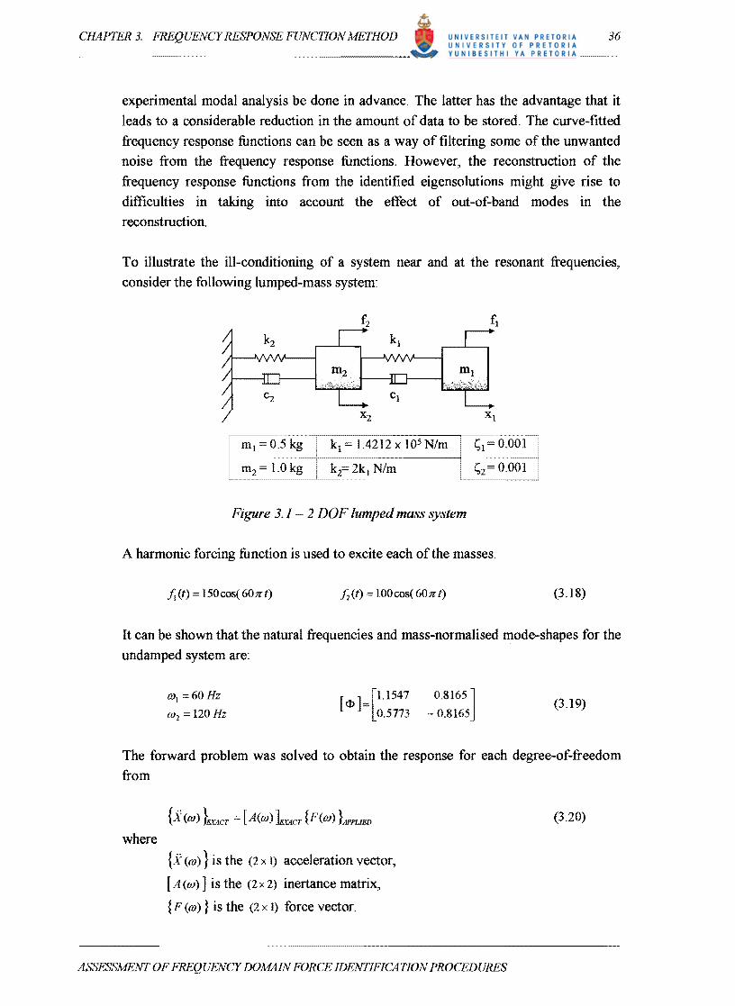

CHAPTER 3 FREQUENCY RESPONSE FUNCTION METHOD
iii~ 2Z -
S - ~ ~~
bil
8 lt1)
c Po
~ -
M pound
50 - Applied
+ Estimated +
0
+
-50 0 20 40 60 80 100 120 140
200
100
0
-100
-200 o
mn
20 40
+
ffit
60 80 100 120
Frequency [Hz]
Figure 33 - Applied and estimatedforce no 2 for the 2 DOF
lumped-mass system in the frequency domain
45
4
35
3
2S
140
05 --___ --____ -L-IL ___ ---________ -
o so 100 150 200 2S0 Frequency [Hz]
Figure 34 - Force Error Norm (FEN) of the estimatedforces
V indicates the 2 DOF systems resonant frequencies
ASSESSMENT OF FREQUENCY DOMAIN FORCE IDENTIFICA TION PROCEDURES
40
CHAPTER 3 FREQUENCY RESPONSE FUNCTION METHOD 41
33 SIGNIFICANCE OF THE CONDITION NUMBER
In the previous section the effect of noise in the force identification was introduced
Consequently errors will always be present in the measurements In this section it is
suggested that the condition number of the frequency response function matrix serves
as a measure of the sensitivity of the pseudo-inverse
Again consider the 2 DOF lumped-mass system This time the system was subjected
to randomly generated forces with uniform distribution on the interval [-1 1] The
responses were obtained utilising the forward problem The contaminated frequency
response function matrix was generated through the perturbation of the modal parameters as previously described Finally the inverse problem was solved to obtain
the force estimates The above procedure was repeated 100 times In each run new
random variables were generated Figure 35 represents the average FEN Ff(OJ) for
these 100 runs
r-
~ -
lt
g OIl pound
4_----_------~------_------_----_------~
35
3
25
2
l L-----~-------L------~------L-----~------~
o 50 100 150 200 250 300
Frequency [Hz]
Figure 35 - A verage Foree Error Norm of estimatedforees
for the 2 DOF lumped-mass system
Golub and Van Loan (1989) describe the error propagation using the condition
number of the matrix to be inverted as an error boundary for perturbation of linear
systems of equations Referring to the above case where only the frequency response
function matrix was perturbated errors in the calculation of F(OJ) will be restricted
by
ASSESSMENT OF FREQUENCY DOMAIN FORCE IDENTIFICA TION PROCEDURES
CHAPTER 3 FREQUENCY RESPONSE FUNCTION METHOD
where
II F (OJ) - fr (OJ) 112 lt K ([ H ]) 2 II [ IiH (OJ) ] 11 2 II F(OJ) II 2 - 2 II[H(OJ) ]11 2
F(OJ) is the actual force vector
hOJ) is the estimated force vector
K 2([ H]) is the condition number of [H ]
[oH(OJ)] is the difference between the actual and perturbated [H]
11middot11 2 is the vector 2-norm
42
(327)
Similar expressions could be obtained for perturbation of the response X (OJ)
Unfortunately these expressions are of little practical use since the actual force and response are unknown
It was suggested that the condition number of the matrix to be inverted should be
used as a measure of the sensitivity of the pseudo-inverse (Starkey and Merrill 1989)
Although the exact magnitude of the error bound of the system at a particular
frequency remains unknown the condition number enables one to comment on the reliability of the force estimates within a given frequency range A high condition
number indicates that the columns of the frequency response function are linearly or
almost linearly dependent ie rank deficient This can result in large errors in the identified forces Conversely a condition number close to unity indicates that the
columns of the frequency response function are almost mutually perpendicular One
should not expect any large amplification of the measurement noise when inverting
the frequency response function matrix Figure 36 shows the condition number of the
frequency response function matrix for the 2 DOF lumped-mass system From this it
is evident that the condition number follows the same trend as the relative error in the
force estimates given in Figure 35
ASSESSMENT OF FREQUENCY DOMAIN FORCE IDENTIFICA TlON PROCEDURES
CHAPTER 3 FREQUENCY RESPONSE FUNCTION METHOD
tS -0 I 0 0
~ 00 9
35
3
25
2
15
05
50 100
~------
150 Frequency [Hz]
200 250 300
Figure 36 - Condition number of frequency response function matrix
43
In the next half of this section we would like to investigate the factors that have an
iniluence on the value of the condition number A more complex structure will be
considered for this purpose
A Finite Element Model (FEM) of a freely supported beam was constructed Ten
equally spaced beam elements were used to simulate the 2 metres long beam The
model was restricted to two dimensions since only the transverse bending modes
were of interest for which the natural frequencies and normal modes were obtained solving the eigenvalue problem The first eight bending modes were used in the
reconstruction of the frequency response function matrix of which the first three
modes were the rigid body modes of the beam A uniform damping factor of 0001
was chosen Each node point was considered as a possible sensor location
Nodes
2 3 4 5 6 7 8 9 10 11
1 1
I ~ I 2m
Cross section
z 1254 mm
I ~ I
508 mm
Figure 3 7 - FEM offree-free beam and response locations
ASSESSMENT OF FREQUENCY DOMAIN FORCE IDENTIFICATION PROCEDURES
44 CHAPTER 3 FREQUENCY RESPONSE HINCTION METHOD
331 Effect of the Number of Forces
Eleven response measurements were taken and four sets of excitation forces were
applied to the beam These sets consisted of 12 3 and 4 forces respectively and are
shown in Figure 38
Nodes
1 2 3 4 5 6 7 8 9 10 11
Figure 38 - FfM offree-free beam andforce locations
Figure 39 shows the condition number of the frequency response function matrix for
each of these sets It is evident from the results that the condition number increases
drastically as the number of force predictions increase The condition number for a
single force prediction is equal to unity over the entire frequency range If an
additional force is added it implies that the column corresponding the force location
be included in the frequency response function matrix which in tum increases the
condition number of the matrix The number of force predictions is however limited
by the number ofmodes included in the analysis (Fabunmi 1986)
332 Effect of the Damping
The effect of the damping on the condition number was evaluated next Only three
forces were applied while still measuring eleven responses From Figure 310 one
notices that the condition number varies for different modal damping factors In fact
as the damping factors increase the condition number decreases especially at the
beams resonances This can be attributed to higher modal overlap due to the higher
damping It was mentioned earlier that at a resonant frequency the systems response
is dominated by that particular mode In a system with higher damping the
neighbouring modes have a larger contribution to the response of the system at that
frequency
333 Effect of the Number of Response Measurements
Figure 311 shows the condition number as a function of the number of response
measurements across the frequency range of interest The beam is once again
subjected to three forces while considering 3 (locations 3 7 and 11)6 (locations 2 3
ASSESSMEWT OF FREQUENCY DOMAIN FORCE IDENTIFICATION PROCEDURES
45 CHAPTER 3 FREQUENCY RESPONSE FUNCTION METHOD
5 7 9 and 11) and 9 (locations 2 345 7 8 9 10 and 11) response measurements respectively
The results show that there is a significant improvement in the condition number by increasing the number of response measurements Since there is a direct relation
between the condition number and force error over-determination will improve the
force estimates as well Adding a response measurement implies that an additional row and thus a new equation is added to the frequency response function matrix
Mas et al (1994) showed that the ratio of the number of response measurements to
the number of force predictions should preferably be greater than or equal to 3 (ie
nm 23)
334 EtTect of the Response Type
Both accelerometers and strain gauges have been employed by Hillary and Ewins (1984) to determine sinusoidal forces on a uniform cantilever beam The strain
responses gave more accurate force estimates since the strain responses are more influenced by the higher modes at low frequencies Han and Wicks (1990) also studied the application of displacement slope and strain measurements From both these studies it is evident that proper selection of the measurement type can improve
the condition of the frequency response function matrix and hence obtain better force predictions
335 Conclusion
It is suggested that the condition number of the frequency response function matrix serves as a measure of the sensitivity of the pseudo-inverse The frequency response function matrix needs to be inverted at each discrete frequency and as a result the condition number varies with frequency Large condition numbers exist near and at
the systems resonances
The condition number of the pseudo-inverse is a function of the number of response points included The number of force predictions systems damping as well as the selection ofthe response type also influence the condition number
ASSElSMENT OF FREQUENCY DOMAIN FORCE IDENTIFICATION PROCEDURES
CHAPTER 3 FREQUENCY RESPONSE FUNCTION METHOD
sect
1
sv
Sri --------------------------~----_--------_--~
45
4
35
l 0 1 ~
o 50 100 150 200 250 300 350 400 450 500
Frequency [Hz]
Figure 39 - Effect of the number of forces on the condition number
sect 0 sect lt)
0
i
4
35
3
25
2
15
05
- S=OmiddotOOI S=Omiddot05
- S=OmiddotI
~ L ~ -- 1 ~ i~~ -------j J~ ~~
OLI __ ~ ________ _L __ ~ ____ ~ __ _L __ ~L_ ______ _L __ ~
o 50 100 150 200 250 300 350 400 450 500
Frequency [Hz]
Figure 310 - Effect of the damping on the condition number
ASSESSMENT OF FREQUENCY DOA1AIN FORCE DENTIFICA TION PROCEDURES
46
CHAPTER 3 FREQUENCY RESPONSE FUNCTION METHOD
451 I
4
35
3
~ 25 sect ~ 2
00 oS
00
~
- 3 Responses 6 Responses
- 9 Responses
50 100 150 200 250 300 350 400 450 500
Frequency [Hz]
Figure 3 J J - Effect ~f the number of response measurements
on the condition number
ASSESSAfENT OF FREQUENCY DOMAIN FORCE IDENTIFICATION PROCEDURES
47
48 CHAPTER 3 FREQUENCY RESPONSE FUNCTION METHOD
34 NUMERICAL STUDY OF A FREE-FREE BEAM
This section examines the different matrix decomposition and regularisation methods
employed for the calculation of the pseudo-inverse For this purpose it was decided to
continue using the FEM of the freely supported aluminium beam as introduced in
Section 33
The eigenvalue problem was solved to obtain the natural frequencies and mode
shapes In addition to the RBM five bending modes were in the chosen frequency
range of 0 to 500 Hz The natural frequencies and mode shapes were taken as the
exact values A proportional damping model was assumed with values obtained
from the experimental modal analysis performed on a similar beam
The beam was then subjected to two simultaneous harmonic forces applied at positions 5 and 11 with forcing frequencies of 220 Hz and 140 Hz respectively The frequency content of the force signals was not determined with an FFT algorithm
thus presenting zero amplitude values in the frequency range except at the discrete
forcing frequencies
The exact response at each of the eleven sensor locations was calculated from
X(01) EUCT = [A(01) bCT F(01) APPLIED (328)
where
x (01) is the (11 xl) acceleration vector
[A(01)] is the (11 x 2) inertance matrix
F(01) is the (2 x 1) force vector
The [A(01)] matrix was constructed from the RBM and five bending modes while
omitting the residual terms The response and modal parameters were perturbated as
described in Section 32 to resemble experimental data Successively the force
identification problem was solved while including only six response locations
(positions 13569 and 11) in the analysis
(329)
where
() denotes the contaminated values
Figure 3 12 shows the effect of the perturbation analysis on the reconstructed
inertance matrix lA(01) j
ASSESSMENT OF FREQUENCY DOMAIN FORCE IDENTIFICATION PROCEDURES
49 CHAPTER 3 FREQUENCY RESPONSE FUNCTION AfETHOD
Each of the previously explained pseudo-inverse methods was employed to evaluate their ability to correctly determine the two harmonic forces
A major difficulty associated with the Tikhonov regularisation is the choice of the
regularisation parameter fi (Da Silva and Rade 1999) The value of this parameter
was obtained from using the L-curve (Hansen and OLeary 1991) The L-curve is a
plot of the semi-norm II [i ]fr II as a function of the residual norm II [H Jfr - x II for various values of fi The comer of the L-curve is identified and the corresponding
regularisation parameter fi is returned This procedure has to be performed at each
discrete frequency line and a result is computationally very expensive
The results of the analysis are presented in Table 32 Only the Tikhonov regularisation failed to predict the two forces correctly This constraint optimisation
algorithm identified the force applied at position 11 correctly but calculated a significant force amplitude with the same frequency content as the force applied at node 11 at the other force location position 5 Furthermore it also under-estimated
the force at node 5 Increasing the number of response locations had no improvement on the result
Table 32 - Force results othe different matrix decomposition
and regularisation methods
1p1[N] IFzl [N]
Applied Force amplitudes
10000 0
0 23000
Singular Value Decomposition QR Decomposition Moore-Penrose
Tikhonov Regularisation
9338 9338 9338
52139
21432
21432 21432 19512
Next the author evaluated the force identification process for the entire frequency
range In this case the frequency content of the harmonic force time signals was determined with an FFT -algorithm thus presenting non-zero values in the frequency range considered Figure 313 illustrates the ill-conditioning of the force estimates at
the resonant frequencies of the beam The ill-conditioning in this particular case is a result of the perturbation analysis the FEM approximations and the FFT -algorithms Changing the excitation points on the beam produced the same trends Once again the
Tikhonov regularisation produced poorer results than the other methods The Singular Value Decomposition QR Decomposition and Moore-Penrose pseudo-inverse produced exactly the same results
ASSESSAfENT OF FREQUENCY DOMAINFORCE IDENTIFICATION PROCEDURES
-- --- ---
50 CHAPTER 3 FREQUENCY RESPONSE FUNCTION METHOD
In view of the above-mentioned the author decided to use the SVD from here onwards
for the calculation of the pseudo-inverse matrix The motivation being the ease of the
implementation of this algorithm in the Matlab environment Another advantage of
the SVD is the ability to ascertain the rank of a matrix and to truncate the singular
values accordingly
Position 9 105
~ i 8 10deg - j ~ U s
200
100
bii 8 c Po
-100
-200 50 100 - middot i)~--middot-2oo 250 300 350 400 450 50o
0 middot -FfequeBCyenl~l- -- shy --- shy
i
i
i
0 -J -----
-- I I
i I j10-5
0 50 IOq 150 200 250 300 350 400 450 500 Frequency [Hz]
shyLshy--=-~- ~
--~--
V[0 [
70 80 jO 100 llO 120 ]10 140
70 SO 90 100 110 120 IJO 140 Frequency IHzI
(J
-50
-100
-15U
-200
l I I
II I I I I
Figure 312 - Comparison ~f the exact andperturbated inertance
frequency response function
ASSESSMENT OF FREQUENCY DOMAIN FORCE IDENTIFICATION PROCEDURES
51 CHAPTER 3 FREQUENCY RESPONSE FUNCTION METHOD
50
ON
~ l ~Zshy-3~ - ~ ~-- -100
-150 0 150 200 250 300 350 400 450 500
~
-5ol
50 100
50 100 150 200 250 300 350 400 450 500
Frequency [Hz]
50
-100 o
V V V V
~I I~J
- Applied SVD
- MP - QR
TR
11I r
Figure 313 - Comparison ofthe different decomposition and
regularisation methods V indicates the resonant frequencies
ASSESSMENT OF FREQUENCY DOlvfAIN FORCE IDENTIFICATION PROCEDURES
shy

CHAPTER 3 FREQUENCY RESPONSE FUNCTION METHOD
where
II F (OJ) - fr (OJ) 112 lt K ([ H ]) 2 II [ IiH (OJ) ] 11 2 II F(OJ) II 2 - 2 II[H(OJ) ]11 2
F(OJ) is the actual force vector
hOJ) is the estimated force vector
K 2([ H]) is the condition number of [H ]
[oH(OJ)] is the difference between the actual and perturbated [H]
11middot11 2 is the vector 2-norm
42
(327)
Similar expressions could be obtained for perturbation of the response X (OJ)
Unfortunately these expressions are of little practical use since the actual force and response are unknown
It was suggested that the condition number of the matrix to be inverted should be
used as a measure of the sensitivity of the pseudo-inverse (Starkey and Merrill 1989)
Although the exact magnitude of the error bound of the system at a particular
frequency remains unknown the condition number enables one to comment on the reliability of the force estimates within a given frequency range A high condition
number indicates that the columns of the frequency response function are linearly or
almost linearly dependent ie rank deficient This can result in large errors in the identified forces Conversely a condition number close to unity indicates that the
columns of the frequency response function are almost mutually perpendicular One
should not expect any large amplification of the measurement noise when inverting
the frequency response function matrix Figure 36 shows the condition number of the
frequency response function matrix for the 2 DOF lumped-mass system From this it
is evident that the condition number follows the same trend as the relative error in the
force estimates given in Figure 35
ASSESSMENT OF FREQUENCY DOMAIN FORCE IDENTIFICA TlON PROCEDURES
CHAPTER 3 FREQUENCY RESPONSE FUNCTION METHOD
tS -0 I 0 0
~ 00 9
35
3
25
2
15
05
50 100
~------
150 Frequency [Hz]
200 250 300
Figure 36 - Condition number of frequency response function matrix
43
In the next half of this section we would like to investigate the factors that have an
iniluence on the value of the condition number A more complex structure will be
considered for this purpose
A Finite Element Model (FEM) of a freely supported beam was constructed Ten
equally spaced beam elements were used to simulate the 2 metres long beam The
model was restricted to two dimensions since only the transverse bending modes
were of interest for which the natural frequencies and normal modes were obtained solving the eigenvalue problem The first eight bending modes were used in the
reconstruction of the frequency response function matrix of which the first three
modes were the rigid body modes of the beam A uniform damping factor of 0001
was chosen Each node point was considered as a possible sensor location
Nodes
2 3 4 5 6 7 8 9 10 11
1 1
I ~ I 2m
Cross section
z 1254 mm
I ~ I
508 mm
Figure 3 7 - FEM offree-free beam and response locations
ASSESSMENT OF FREQUENCY DOMAIN FORCE IDENTIFICATION PROCEDURES
44 CHAPTER 3 FREQUENCY RESPONSE HINCTION METHOD
331 Effect of the Number of Forces
Eleven response measurements were taken and four sets of excitation forces were
applied to the beam These sets consisted of 12 3 and 4 forces respectively and are
shown in Figure 38
Nodes
1 2 3 4 5 6 7 8 9 10 11
Figure 38 - FfM offree-free beam andforce locations
Figure 39 shows the condition number of the frequency response function matrix for
each of these sets It is evident from the results that the condition number increases
drastically as the number of force predictions increase The condition number for a
single force prediction is equal to unity over the entire frequency range If an
additional force is added it implies that the column corresponding the force location
be included in the frequency response function matrix which in tum increases the
condition number of the matrix The number of force predictions is however limited
by the number ofmodes included in the analysis (Fabunmi 1986)
332 Effect of the Damping
The effect of the damping on the condition number was evaluated next Only three
forces were applied while still measuring eleven responses From Figure 310 one
notices that the condition number varies for different modal damping factors In fact
as the damping factors increase the condition number decreases especially at the
beams resonances This can be attributed to higher modal overlap due to the higher
damping It was mentioned earlier that at a resonant frequency the systems response
is dominated by that particular mode In a system with higher damping the
neighbouring modes have a larger contribution to the response of the system at that
frequency
333 Effect of the Number of Response Measurements
Figure 311 shows the condition number as a function of the number of response
measurements across the frequency range of interest The beam is once again
subjected to three forces while considering 3 (locations 3 7 and 11)6 (locations 2 3
ASSESSMEWT OF FREQUENCY DOMAIN FORCE IDENTIFICATION PROCEDURES
45 CHAPTER 3 FREQUENCY RESPONSE FUNCTION METHOD
5 7 9 and 11) and 9 (locations 2 345 7 8 9 10 and 11) response measurements respectively
The results show that there is a significant improvement in the condition number by increasing the number of response measurements Since there is a direct relation
between the condition number and force error over-determination will improve the
force estimates as well Adding a response measurement implies that an additional row and thus a new equation is added to the frequency response function matrix
Mas et al (1994) showed that the ratio of the number of response measurements to
the number of force predictions should preferably be greater than or equal to 3 (ie
nm 23)
334 EtTect of the Response Type
Both accelerometers and strain gauges have been employed by Hillary and Ewins (1984) to determine sinusoidal forces on a uniform cantilever beam The strain
responses gave more accurate force estimates since the strain responses are more influenced by the higher modes at low frequencies Han and Wicks (1990) also studied the application of displacement slope and strain measurements From both these studies it is evident that proper selection of the measurement type can improve
the condition of the frequency response function matrix and hence obtain better force predictions
335 Conclusion
It is suggested that the condition number of the frequency response function matrix serves as a measure of the sensitivity of the pseudo-inverse The frequency response function matrix needs to be inverted at each discrete frequency and as a result the condition number varies with frequency Large condition numbers exist near and at
the systems resonances
The condition number of the pseudo-inverse is a function of the number of response points included The number of force predictions systems damping as well as the selection ofthe response type also influence the condition number
ASSElSMENT OF FREQUENCY DOMAIN FORCE IDENTIFICATION PROCEDURES
CHAPTER 3 FREQUENCY RESPONSE FUNCTION METHOD
sect
1
sv
Sri --------------------------~----_--------_--~
45
4
35
l 0 1 ~
o 50 100 150 200 250 300 350 400 450 500
Frequency [Hz]
Figure 39 - Effect of the number of forces on the condition number
sect 0 sect lt)
0
i
4
35
3
25
2
15
05
- S=OmiddotOOI S=Omiddot05
- S=OmiddotI
~ L ~ -- 1 ~ i~~ -------j J~ ~~
OLI __ ~ ________ _L __ ~ ____ ~ __ _L __ ~L_ ______ _L __ ~
o 50 100 150 200 250 300 350 400 450 500
Frequency [Hz]
Figure 310 - Effect of the damping on the condition number
ASSESSMENT OF FREQUENCY DOA1AIN FORCE DENTIFICA TION PROCEDURES
46
CHAPTER 3 FREQUENCY RESPONSE FUNCTION METHOD
451 I
4
35
3
~ 25 sect ~ 2
00 oS
00
~
- 3 Responses 6 Responses
- 9 Responses
50 100 150 200 250 300 350 400 450 500
Frequency [Hz]
Figure 3 J J - Effect ~f the number of response measurements
on the condition number
ASSESSAfENT OF FREQUENCY DOMAIN FORCE IDENTIFICATION PROCEDURES
47
48 CHAPTER 3 FREQUENCY RESPONSE FUNCTION METHOD
34 NUMERICAL STUDY OF A FREE-FREE BEAM
This section examines the different matrix decomposition and regularisation methods
employed for the calculation of the pseudo-inverse For this purpose it was decided to
continue using the FEM of the freely supported aluminium beam as introduced in
Section 33
The eigenvalue problem was solved to obtain the natural frequencies and mode
shapes In addition to the RBM five bending modes were in the chosen frequency
range of 0 to 500 Hz The natural frequencies and mode shapes were taken as the
exact values A proportional damping model was assumed with values obtained
from the experimental modal analysis performed on a similar beam
The beam was then subjected to two simultaneous harmonic forces applied at positions 5 and 11 with forcing frequencies of 220 Hz and 140 Hz respectively The frequency content of the force signals was not determined with an FFT algorithm
thus presenting zero amplitude values in the frequency range except at the discrete
forcing frequencies
The exact response at each of the eleven sensor locations was calculated from
X(01) EUCT = [A(01) bCT F(01) APPLIED (328)
where
x (01) is the (11 xl) acceleration vector
[A(01)] is the (11 x 2) inertance matrix
F(01) is the (2 x 1) force vector
The [A(01)] matrix was constructed from the RBM and five bending modes while
omitting the residual terms The response and modal parameters were perturbated as
described in Section 32 to resemble experimental data Successively the force
identification problem was solved while including only six response locations
(positions 13569 and 11) in the analysis
(329)
where
() denotes the contaminated values
Figure 3 12 shows the effect of the perturbation analysis on the reconstructed
inertance matrix lA(01) j
ASSESSMENT OF FREQUENCY DOMAIN FORCE IDENTIFICATION PROCEDURES
49 CHAPTER 3 FREQUENCY RESPONSE FUNCTION AfETHOD
Each of the previously explained pseudo-inverse methods was employed to evaluate their ability to correctly determine the two harmonic forces
A major difficulty associated with the Tikhonov regularisation is the choice of the
regularisation parameter fi (Da Silva and Rade 1999) The value of this parameter
was obtained from using the L-curve (Hansen and OLeary 1991) The L-curve is a
plot of the semi-norm II [i ]fr II as a function of the residual norm II [H Jfr - x II for various values of fi The comer of the L-curve is identified and the corresponding
regularisation parameter fi is returned This procedure has to be performed at each
discrete frequency line and a result is computationally very expensive
The results of the analysis are presented in Table 32 Only the Tikhonov regularisation failed to predict the two forces correctly This constraint optimisation
algorithm identified the force applied at position 11 correctly but calculated a significant force amplitude with the same frequency content as the force applied at node 11 at the other force location position 5 Furthermore it also under-estimated
the force at node 5 Increasing the number of response locations had no improvement on the result
Table 32 - Force results othe different matrix decomposition
and regularisation methods
1p1[N] IFzl [N]
Applied Force amplitudes
10000 0
0 23000
Singular Value Decomposition QR Decomposition Moore-Penrose
Tikhonov Regularisation
9338 9338 9338
52139
21432
21432 21432 19512
Next the author evaluated the force identification process for the entire frequency
range In this case the frequency content of the harmonic force time signals was determined with an FFT -algorithm thus presenting non-zero values in the frequency range considered Figure 313 illustrates the ill-conditioning of the force estimates at
the resonant frequencies of the beam The ill-conditioning in this particular case is a result of the perturbation analysis the FEM approximations and the FFT -algorithms Changing the excitation points on the beam produced the same trends Once again the
Tikhonov regularisation produced poorer results than the other methods The Singular Value Decomposition QR Decomposition and Moore-Penrose pseudo-inverse produced exactly the same results
ASSESSAfENT OF FREQUENCY DOMAINFORCE IDENTIFICATION PROCEDURES
-- --- ---
50 CHAPTER 3 FREQUENCY RESPONSE FUNCTION METHOD
In view of the above-mentioned the author decided to use the SVD from here onwards
for the calculation of the pseudo-inverse matrix The motivation being the ease of the
implementation of this algorithm in the Matlab environment Another advantage of
the SVD is the ability to ascertain the rank of a matrix and to truncate the singular
values accordingly
Position 9 105
~ i 8 10deg - j ~ U s
200
100
bii 8 c Po
-100
-200 50 100 - middot i)~--middot-2oo 250 300 350 400 450 50o
0 middot -FfequeBCyenl~l- -- shy --- shy
i
i
i
0 -J -----
-- I I
i I j10-5
0 50 IOq 150 200 250 300 350 400 450 500 Frequency [Hz]
shyLshy--=-~- ~
--~--
V[0 [
70 80 jO 100 llO 120 ]10 140
70 SO 90 100 110 120 IJO 140 Frequency IHzI
(J
-50
-100
-15U
-200
l I I
II I I I I
Figure 312 - Comparison ~f the exact andperturbated inertance
frequency response function
ASSESSMENT OF FREQUENCY DOMAIN FORCE IDENTIFICATION PROCEDURES
51 CHAPTER 3 FREQUENCY RESPONSE FUNCTION METHOD
50
ON
~ l ~Zshy-3~ - ~ ~-- -100
-150 0 150 200 250 300 350 400 450 500
~
-5ol
50 100
50 100 150 200 250 300 350 400 450 500
Frequency [Hz]
50
-100 o
V V V V
~I I~J
- Applied SVD
- MP - QR
TR
11I r
Figure 313 - Comparison ofthe different decomposition and
regularisation methods V indicates the resonant frequencies
ASSESSMENT OF FREQUENCY DOlvfAIN FORCE IDENTIFICATION PROCEDURES
shy

CHAPTER 3 FREQUENCY RESPONSE FUNCTION METHOD
tS -0 I 0 0
~ 00 9
35
3
25
2
15
05
50 100
~------
150 Frequency [Hz]
200 250 300
Figure 36 - Condition number of frequency response function matrix
43
In the next half of this section we would like to investigate the factors that have an
iniluence on the value of the condition number A more complex structure will be
considered for this purpose
A Finite Element Model (FEM) of a freely supported beam was constructed Ten
equally spaced beam elements were used to simulate the 2 metres long beam The
model was restricted to two dimensions since only the transverse bending modes
were of interest for which the natural frequencies and normal modes were obtained solving the eigenvalue problem The first eight bending modes were used in the
reconstruction of the frequency response function matrix of which the first three
modes were the rigid body modes of the beam A uniform damping factor of 0001
was chosen Each node point was considered as a possible sensor location
Nodes
2 3 4 5 6 7 8 9 10 11
1 1
I ~ I 2m
Cross section
z 1254 mm
I ~ I
508 mm
Figure 3 7 - FEM offree-free beam and response locations
ASSESSMENT OF FREQUENCY DOMAIN FORCE IDENTIFICATION PROCEDURES
44 CHAPTER 3 FREQUENCY RESPONSE HINCTION METHOD
331 Effect of the Number of Forces
Eleven response measurements were taken and four sets of excitation forces were
applied to the beam These sets consisted of 12 3 and 4 forces respectively and are
shown in Figure 38
Nodes
1 2 3 4 5 6 7 8 9 10 11
Figure 38 - FfM offree-free beam andforce locations
Figure 39 shows the condition number of the frequency response function matrix for
each of these sets It is evident from the results that the condition number increases
drastically as the number of force predictions increase The condition number for a
single force prediction is equal to unity over the entire frequency range If an
additional force is added it implies that the column corresponding the force location
be included in the frequency response function matrix which in tum increases the
condition number of the matrix The number of force predictions is however limited
by the number ofmodes included in the analysis (Fabunmi 1986)
332 Effect of the Damping
The effect of the damping on the condition number was evaluated next Only three
forces were applied while still measuring eleven responses From Figure 310 one
notices that the condition number varies for different modal damping factors In fact
as the damping factors increase the condition number decreases especially at the
beams resonances This can be attributed to higher modal overlap due to the higher
damping It was mentioned earlier that at a resonant frequency the systems response
is dominated by that particular mode In a system with higher damping the
neighbouring modes have a larger contribution to the response of the system at that
frequency
333 Effect of the Number of Response Measurements
Figure 311 shows the condition number as a function of the number of response
measurements across the frequency range of interest The beam is once again
subjected to three forces while considering 3 (locations 3 7 and 11)6 (locations 2 3
ASSESSMEWT OF FREQUENCY DOMAIN FORCE IDENTIFICATION PROCEDURES
45 CHAPTER 3 FREQUENCY RESPONSE FUNCTION METHOD
5 7 9 and 11) and 9 (locations 2 345 7 8 9 10 and 11) response measurements respectively
The results show that there is a significant improvement in the condition number by increasing the number of response measurements Since there is a direct relation
between the condition number and force error over-determination will improve the
force estimates as well Adding a response measurement implies that an additional row and thus a new equation is added to the frequency response function matrix
Mas et al (1994) showed that the ratio of the number of response measurements to
the number of force predictions should preferably be greater than or equal to 3 (ie
nm 23)
334 EtTect of the Response Type
Both accelerometers and strain gauges have been employed by Hillary and Ewins (1984) to determine sinusoidal forces on a uniform cantilever beam The strain
responses gave more accurate force estimates since the strain responses are more influenced by the higher modes at low frequencies Han and Wicks (1990) also studied the application of displacement slope and strain measurements From both these studies it is evident that proper selection of the measurement type can improve
the condition of the frequency response function matrix and hence obtain better force predictions
335 Conclusion
It is suggested that the condition number of the frequency response function matrix serves as a measure of the sensitivity of the pseudo-inverse The frequency response function matrix needs to be inverted at each discrete frequency and as a result the condition number varies with frequency Large condition numbers exist near and at
the systems resonances
The condition number of the pseudo-inverse is a function of the number of response points included The number of force predictions systems damping as well as the selection ofthe response type also influence the condition number
ASSElSMENT OF FREQUENCY DOMAIN FORCE IDENTIFICATION PROCEDURES
CHAPTER 3 FREQUENCY RESPONSE FUNCTION METHOD
sect
1
sv
Sri --------------------------~----_--------_--~
45
4
35
l 0 1 ~
o 50 100 150 200 250 300 350 400 450 500
Frequency [Hz]
Figure 39 - Effect of the number of forces on the condition number
sect 0 sect lt)
0
i
4
35
3
25
2
15
05
- S=OmiddotOOI S=Omiddot05
- S=OmiddotI
~ L ~ -- 1 ~ i~~ -------j J~ ~~
OLI __ ~ ________ _L __ ~ ____ ~ __ _L __ ~L_ ______ _L __ ~
o 50 100 150 200 250 300 350 400 450 500
Frequency [Hz]
Figure 310 - Effect of the damping on the condition number
ASSESSMENT OF FREQUENCY DOA1AIN FORCE DENTIFICA TION PROCEDURES
46
CHAPTER 3 FREQUENCY RESPONSE FUNCTION METHOD
451 I
4
35
3
~ 25 sect ~ 2
00 oS
00
~
- 3 Responses 6 Responses
- 9 Responses
50 100 150 200 250 300 350 400 450 500
Frequency [Hz]
Figure 3 J J - Effect ~f the number of response measurements
on the condition number
ASSESSAfENT OF FREQUENCY DOMAIN FORCE IDENTIFICATION PROCEDURES
47
48 CHAPTER 3 FREQUENCY RESPONSE FUNCTION METHOD
34 NUMERICAL STUDY OF A FREE-FREE BEAM
This section examines the different matrix decomposition and regularisation methods
employed for the calculation of the pseudo-inverse For this purpose it was decided to
continue using the FEM of the freely supported aluminium beam as introduced in
Section 33
The eigenvalue problem was solved to obtain the natural frequencies and mode
shapes In addition to the RBM five bending modes were in the chosen frequency
range of 0 to 500 Hz The natural frequencies and mode shapes were taken as the
exact values A proportional damping model was assumed with values obtained
from the experimental modal analysis performed on a similar beam
The beam was then subjected to two simultaneous harmonic forces applied at positions 5 and 11 with forcing frequencies of 220 Hz and 140 Hz respectively The frequency content of the force signals was not determined with an FFT algorithm
thus presenting zero amplitude values in the frequency range except at the discrete
forcing frequencies
The exact response at each of the eleven sensor locations was calculated from
X(01) EUCT = [A(01) bCT F(01) APPLIED (328)
where
x (01) is the (11 xl) acceleration vector
[A(01)] is the (11 x 2) inertance matrix
F(01) is the (2 x 1) force vector
The [A(01)] matrix was constructed from the RBM and five bending modes while
omitting the residual terms The response and modal parameters were perturbated as
described in Section 32 to resemble experimental data Successively the force
identification problem was solved while including only six response locations
(positions 13569 and 11) in the analysis
(329)
where
() denotes the contaminated values
Figure 3 12 shows the effect of the perturbation analysis on the reconstructed
inertance matrix lA(01) j
ASSESSMENT OF FREQUENCY DOMAIN FORCE IDENTIFICATION PROCEDURES
49 CHAPTER 3 FREQUENCY RESPONSE FUNCTION AfETHOD
Each of the previously explained pseudo-inverse methods was employed to evaluate their ability to correctly determine the two harmonic forces
A major difficulty associated with the Tikhonov regularisation is the choice of the
regularisation parameter fi (Da Silva and Rade 1999) The value of this parameter
was obtained from using the L-curve (Hansen and OLeary 1991) The L-curve is a
plot of the semi-norm II [i ]fr II as a function of the residual norm II [H Jfr - x II for various values of fi The comer of the L-curve is identified and the corresponding
regularisation parameter fi is returned This procedure has to be performed at each
discrete frequency line and a result is computationally very expensive
The results of the analysis are presented in Table 32 Only the Tikhonov regularisation failed to predict the two forces correctly This constraint optimisation
algorithm identified the force applied at position 11 correctly but calculated a significant force amplitude with the same frequency content as the force applied at node 11 at the other force location position 5 Furthermore it also under-estimated
the force at node 5 Increasing the number of response locations had no improvement on the result
Table 32 - Force results othe different matrix decomposition
and regularisation methods
1p1[N] IFzl [N]
Applied Force amplitudes
10000 0
0 23000
Singular Value Decomposition QR Decomposition Moore-Penrose
Tikhonov Regularisation
9338 9338 9338
52139
21432
21432 21432 19512
Next the author evaluated the force identification process for the entire frequency
range In this case the frequency content of the harmonic force time signals was determined with an FFT -algorithm thus presenting non-zero values in the frequency range considered Figure 313 illustrates the ill-conditioning of the force estimates at
the resonant frequencies of the beam The ill-conditioning in this particular case is a result of the perturbation analysis the FEM approximations and the FFT -algorithms Changing the excitation points on the beam produced the same trends Once again the
Tikhonov regularisation produced poorer results than the other methods The Singular Value Decomposition QR Decomposition and Moore-Penrose pseudo-inverse produced exactly the same results
ASSESSAfENT OF FREQUENCY DOMAINFORCE IDENTIFICATION PROCEDURES
-- --- ---
50 CHAPTER 3 FREQUENCY RESPONSE FUNCTION METHOD
In view of the above-mentioned the author decided to use the SVD from here onwards
for the calculation of the pseudo-inverse matrix The motivation being the ease of the
implementation of this algorithm in the Matlab environment Another advantage of
the SVD is the ability to ascertain the rank of a matrix and to truncate the singular
values accordingly
Position 9 105
~ i 8 10deg - j ~ U s
200
100
bii 8 c Po
-100
-200 50 100 - middot i)~--middot-2oo 250 300 350 400 450 50o
0 middot -FfequeBCyenl~l- -- shy --- shy
i
i
i
0 -J -----
-- I I
i I j10-5
0 50 IOq 150 200 250 300 350 400 450 500 Frequency [Hz]
shyLshy--=-~- ~
--~--
V[0 [
70 80 jO 100 llO 120 ]10 140
70 SO 90 100 110 120 IJO 140 Frequency IHzI
(J
-50
-100
-15U
-200
l I I
II I I I I
Figure 312 - Comparison ~f the exact andperturbated inertance
frequency response function
ASSESSMENT OF FREQUENCY DOMAIN FORCE IDENTIFICATION PROCEDURES
51 CHAPTER 3 FREQUENCY RESPONSE FUNCTION METHOD
50
ON
~ l ~Zshy-3~ - ~ ~-- -100
-150 0 150 200 250 300 350 400 450 500
~
-5ol
50 100
50 100 150 200 250 300 350 400 450 500
Frequency [Hz]
50
-100 o
V V V V
~I I~J
- Applied SVD
- MP - QR
TR
11I r
Figure 313 - Comparison ofthe different decomposition and
regularisation methods V indicates the resonant frequencies
ASSESSMENT OF FREQUENCY DOlvfAIN FORCE IDENTIFICATION PROCEDURES
shy
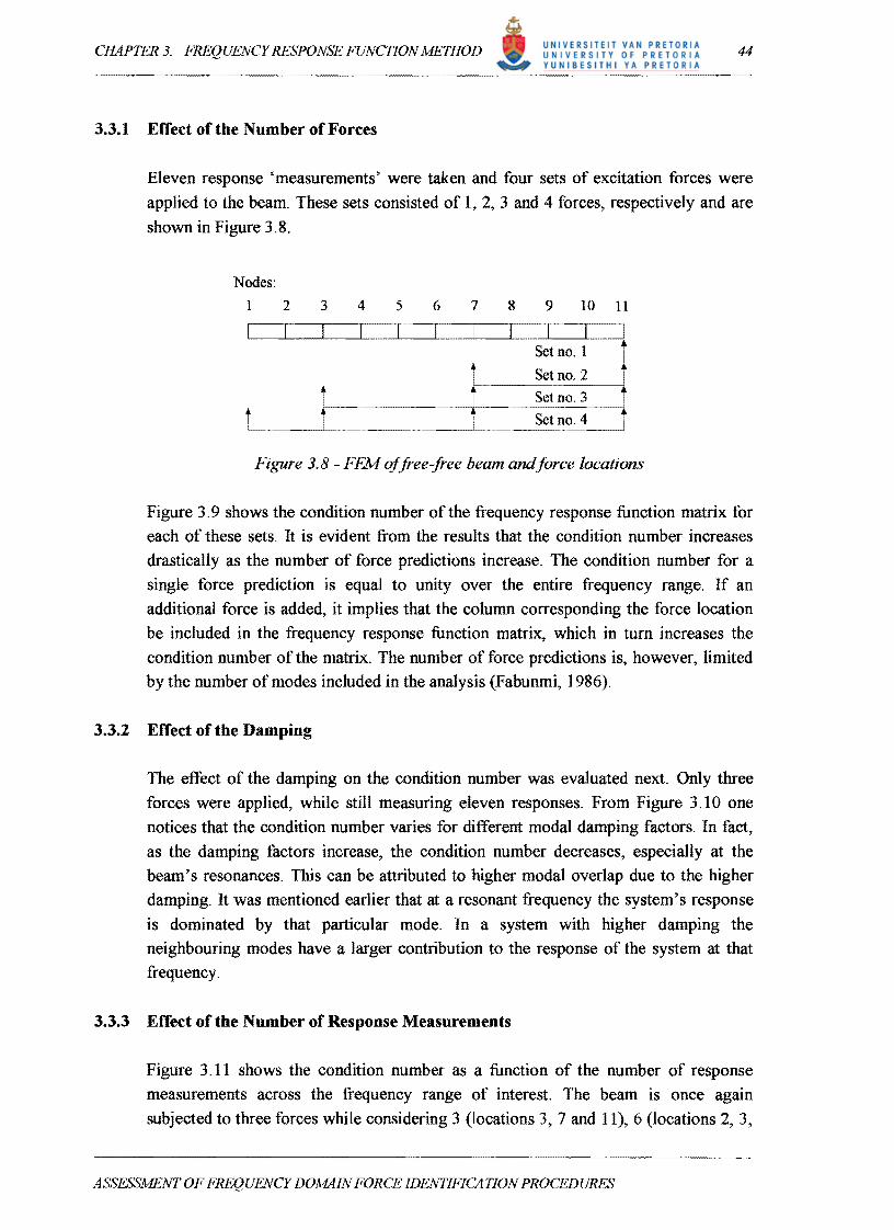

CHAPTER 3 FREQUENCY RESPONSE FUNCTION METHOD
451 I
4
35
3
~ 25 sect ~ 2
00 oS
00
~
- 3 Responses 6 Responses
- 9 Responses
50 100 150 200 250 300 350 400 450 500
Frequency [Hz]
Figure 3 J J - Effect ~f the number of response measurements
on the condition number
ASSESSAfENT OF FREQUENCY DOMAIN FORCE IDENTIFICATION PROCEDURES
47
48 CHAPTER 3 FREQUENCY RESPONSE FUNCTION METHOD
34 NUMERICAL STUDY OF A FREE-FREE BEAM
This section examines the different matrix decomposition and regularisation methods
employed for the calculation of the pseudo-inverse For this purpose it was decided to
continue using the FEM of the freely supported aluminium beam as introduced in
Section 33
The eigenvalue problem was solved to obtain the natural frequencies and mode
shapes In addition to the RBM five bending modes were in the chosen frequency
range of 0 to 500 Hz The natural frequencies and mode shapes were taken as the
exact values A proportional damping model was assumed with values obtained
from the experimental modal analysis performed on a similar beam
The beam was then subjected to two simultaneous harmonic forces applied at positions 5 and 11 with forcing frequencies of 220 Hz and 140 Hz respectively The frequency content of the force signals was not determined with an FFT algorithm
thus presenting zero amplitude values in the frequency range except at the discrete
forcing frequencies
The exact response at each of the eleven sensor locations was calculated from
X(01) EUCT = [A(01) bCT F(01) APPLIED (328)
where
x (01) is the (11 xl) acceleration vector
[A(01)] is the (11 x 2) inertance matrix
F(01) is the (2 x 1) force vector
The [A(01)] matrix was constructed from the RBM and five bending modes while
omitting the residual terms The response and modal parameters were perturbated as
described in Section 32 to resemble experimental data Successively the force
identification problem was solved while including only six response locations
(positions 13569 and 11) in the analysis
(329)
where
() denotes the contaminated values
Figure 3 12 shows the effect of the perturbation analysis on the reconstructed
inertance matrix lA(01) j
ASSESSMENT OF FREQUENCY DOMAIN FORCE IDENTIFICATION PROCEDURES
49 CHAPTER 3 FREQUENCY RESPONSE FUNCTION AfETHOD
Each of the previously explained pseudo-inverse methods was employed to evaluate their ability to correctly determine the two harmonic forces
A major difficulty associated with the Tikhonov regularisation is the choice of the
regularisation parameter fi (Da Silva and Rade 1999) The value of this parameter
was obtained from using the L-curve (Hansen and OLeary 1991) The L-curve is a
plot of the semi-norm II [i ]fr II as a function of the residual norm II [H Jfr - x II for various values of fi The comer of the L-curve is identified and the corresponding
regularisation parameter fi is returned This procedure has to be performed at each
discrete frequency line and a result is computationally very expensive
The results of the analysis are presented in Table 32 Only the Tikhonov regularisation failed to predict the two forces correctly This constraint optimisation
algorithm identified the force applied at position 11 correctly but calculated a significant force amplitude with the same frequency content as the force applied at node 11 at the other force location position 5 Furthermore it also under-estimated
the force at node 5 Increasing the number of response locations had no improvement on the result
Table 32 - Force results othe different matrix decomposition
and regularisation methods
1p1[N] IFzl [N]
Applied Force amplitudes
10000 0
0 23000
Singular Value Decomposition QR Decomposition Moore-Penrose
Tikhonov Regularisation
9338 9338 9338
52139
21432
21432 21432 19512
Next the author evaluated the force identification process for the entire frequency
range In this case the frequency content of the harmonic force time signals was determined with an FFT -algorithm thus presenting non-zero values in the frequency range considered Figure 313 illustrates the ill-conditioning of the force estimates at
the resonant frequencies of the beam The ill-conditioning in this particular case is a result of the perturbation analysis the FEM approximations and the FFT -algorithms Changing the excitation points on the beam produced the same trends Once again the
Tikhonov regularisation produced poorer results than the other methods The Singular Value Decomposition QR Decomposition and Moore-Penrose pseudo-inverse produced exactly the same results
ASSESSAfENT OF FREQUENCY DOMAINFORCE IDENTIFICATION PROCEDURES
-- --- ---
50 CHAPTER 3 FREQUENCY RESPONSE FUNCTION METHOD
In view of the above-mentioned the author decided to use the SVD from here onwards
for the calculation of the pseudo-inverse matrix The motivation being the ease of the
implementation of this algorithm in the Matlab environment Another advantage of
the SVD is the ability to ascertain the rank of a matrix and to truncate the singular
values accordingly
Position 9 105
~ i 8 10deg - j ~ U s
200
100
bii 8 c Po
-100
-200 50 100 - middot i)~--middot-2oo 250 300 350 400 450 50o
0 middot -FfequeBCyenl~l- -- shy --- shy
i
i
i
0 -J -----
-- I I
i I j10-5
0 50 IOq 150 200 250 300 350 400 450 500 Frequency [Hz]
shyLshy--=-~- ~
--~--
V[0 [
70 80 jO 100 llO 120 ]10 140
70 SO 90 100 110 120 IJO 140 Frequency IHzI
(J
-50
-100
-15U
-200
l I I
II I I I I
Figure 312 - Comparison ~f the exact andperturbated inertance
frequency response function
ASSESSMENT OF FREQUENCY DOMAIN FORCE IDENTIFICATION PROCEDURES
51 CHAPTER 3 FREQUENCY RESPONSE FUNCTION METHOD
50
ON
~ l ~Zshy-3~ - ~ ~-- -100
-150 0 150 200 250 300 350 400 450 500
~
-5ol
50 100
50 100 150 200 250 300 350 400 450 500
Frequency [Hz]
50
-100 o
V V V V
~I I~J
- Applied SVD
- MP - QR
TR
11I r
Figure 313 - Comparison ofthe different decomposition and
regularisation methods V indicates the resonant frequencies
ASSESSMENT OF FREQUENCY DOlvfAIN FORCE IDENTIFICATION PROCEDURES
shy


![Circuit Network Analysis - [Chapter5] Transfer function, frequency response, and Bode plot](https://static.fdocuments.net/doc/165x107/55c99800bb61eb45328b47b3/circuit-network-analysis-chapter5-transfer-function-frequency-response.jpg)

