The finite difference methods - Moodle

The finite difference methodsAlain Hebert

[email protected]

Institut de genie nucleaire

Ecole Polytechnique de Montreal

ENE6103: Week 4 The finite difference methods – 1/18

Content (week 4) 1

Discretization of the neutron diffusion equation

Mesh-corner finite differences

Mesh-centered finite differences


Discretization of the diffusion equation 1discretization is the technique we use to transform an algebraic operator into a matrixoperator.

A discretization of the neutron diffusion equation allows its transformation into a matrixsystem that can be solved by standard numerical analysis techniques.

A discretization technique is said to be consistent if the discretization of a Laplaceoperator ∇2φ(r) produces a symmetric, positive-definite and diagonally dominantmatrix.

Consistent discretization techniques are generally based on polynomialapproximation of the neutron flux in each region. Each homogeneous region ofthe reactor can be sub-divided into sub-regions in order to increase the number ofpiecewise polynomials. This operation is called sub-meshing.

A numerical solution of a consistent discretization technique must tend to theexact solution of the differential problem

as the number of sub-regions increases to infinity, for a given order of thepolynomial basis,as the polynomial order of the polynomial basis increases to infinity, for a givennumber of sub-regions.


Discretization of the diffusion equation 2The symmetry of the matrix operator is important to ensure that the discretization of anadjoint differential equation leads to the transposed matrix operator obtained from thediscretization of the direct differential equation.

The positive-definite and diagonally dominant criteria ensure the success of thestandard numerical analysis techniques used to solve the matrix system.

Discretization techniques can be derived from the differential formulation of theneutron diffusion equation by replacing the dependent variable with Taylor’sexpansions or by using a weighted residual approach.

They can also be obtained from a variational formulation by finding a stationary pointof an ad-hoc functional (aka Rayleigh-Ritz method). The choice of the functional isarbitrary, the only condition being that the Euler equations of the functional must beidentical to the neutron diffusion equation with its continuity and boundary conditions.

A discretization technique can be primal if it belongs to the family of mesh-corner finitedifference, or dual if it belongs to the family of mesh-centered finite differencemethods. A discretization technique can be simultaneously primal and dual(primal-dual agreement), a characteristic of superconvergent approximations.

Both mesh-corner and mesh-centered techniques are consistent discretization approachesthat can be obtained from the differential formulation of the neutron diffusion equation.


Mesh-corner finite differences 1The 1D Cartesian mesh-corner finite difference formulation can be derived from thedifferential formulation of the neutron diffusion equation, by replacing the flux derivativeterms in the diffusion equation by finite-difference relations written in terms of the neutronflux values at specific abscissa points.

i-1 i i+1

xi-3/2 x

i-1/2 xi+1/2

xi+3/2

xi-1 x

i+1 xi

∆xi-1 ∆x

i ∆x

i+1

X

region regionregion

In its mesh-corner formulation, the abscissa points where the neutron flux is explicitlycalculated are chosen on the boundary between sub-regions and are numbered as depictedin the figure. We will use Taylor expansions to represent the flux at points xi−3/2 and xi+1/2

in terms of the flux at point xi−1/2 , so that

φ(xi−3/2) = φ(xi−1/2) − ∆xi−1 φ′(x−

i−1/2) +

1

2∆x2

i−1 φ′′(x−

i−1/2)(1)

and

φ(xi+1/2) = φ(xi−1/2) + ∆xi φ′(x+

i−1/2) +

1

2∆x2

i φ′′(x+

i−1/2)(2)

where the energy group index was omitted, in order to simplify the notation.ENE6103: Week 4 The finite difference methods – 5/18

Mesh-corner finite differences 2The neutron current continuity condition at xi−1/2 causes a discontinuity in the firstderivative of the neutron flux at this point:

Di−1 φ′(x−

i−1/2) = Di φ′(x+

i−1/2) .(3)

We multiply Eqs. (1) and (2) by Di−1/∆xi−1 and Di/∆xi, respectively, add the resultingrelations and introduce Eq. (3):

1

2

h

∆xi−1Di−1 φ′′(x−

i−1/2) + ∆xiDi φ′′(x+

i−1/2)i

=Di

∆xi

ˆ

φ(xi+1/2) − φ(xi−1/2)˜

−Di−1

∆xi−1

ˆ

φ(xi−1/2) − φ(xi−3/2)˜

.(4)

Equation (4) is used as a finite difference relation valid for the internal points. We also needrelations valid on boundary points where an albedo boundary condition is imposed:

φ(x3/2) = φ(x1/2) + ∆x1 φ′(x1/2) +1

2∆x2

1 φ′′(x1/2) (left boundary)(5)

φ(xI−1/2) = φ(xI+1/2) − ∆xI φ′(xI+1/2) +1

2∆x2

I φ′′(xI+1/2) (right boundary)(6)


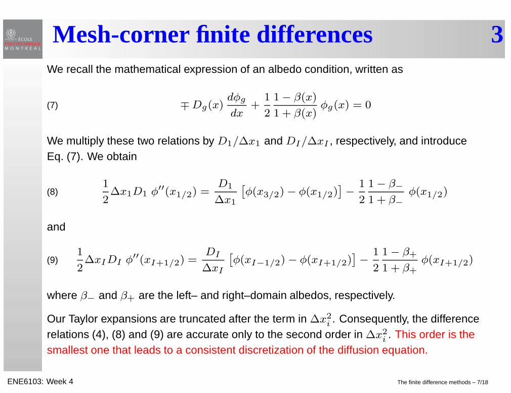
Mesh-corner finite differences 3We recall the mathematical expression of an albedo condition, written as

∓ Dg(x)dφg

dx+

1

2

1 − β(x)

1 + β(x)φg(x) = 0(7)

We multiply these two relations by D1/∆x1 and DI/∆xI , respectively, and introduceEq. (7). We obtain

1

2∆x1D1 φ′′(x1/2) =

D1

∆x1

ˆ

φ(x3/2) − φ(x1/2)˜

−1

2

1 − β−

1 + β−

φ(x1/2)(8)

and

1

2∆xIDI φ′′(xI+1/2) =

DI

∆xI

ˆ

φ(xI−1/2) − φ(xI+1/2)˜

−1

2

1 − β+

1 + β+

φ(xI+1/2)(9)

where β− and β+ are the left– and right–domain albedos, respectively.

Our Taylor expansions are truncated after the term in ∆x2i . Consequently, the difference

relations (4), (8) and (9) are accurate only to the second order in ∆x2i . This order is the

smallest one that leads to a consistent discretization of the diffusion equation.


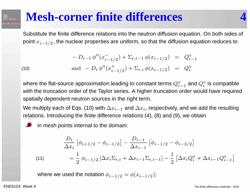
Mesh-corner finite differences 4Substitute the finite difference relations into the neutron diffusion equation. On both sides ofpoint xi−1/2, the nuclear properties are uniform, so that the diffusion equation reduces to

− Di−1 φ′′(x−

i−1/2) + Σr,i−1 φ(xi−1/2) = Q⋄

i−1

and − Di φ′′(x+

i−1/2) + Σr,i φ(xi−1/2) = Q⋄

i(10)

where the flat-source approximation leading to constant terms Q⋄

i−1and Q⋄

i is compatiblewith the truncation order of the Taylor series. A higher truncation order would have requiredspatially dependent neutron sources in the right term.

We multiply each of Eqs. (10) with ∆xi−1 and ∆xi, respectively, and we add the resultingrelations. Introducing the finite difference relations (4), (8) and (9), we obtain

in mesh points internal to the domain:

Di

∆xi

ˆ

φi+1/2 − φi−1/2

˜

−Di−1

∆xi−1

ˆ

φi−1/2 − φi−3/2

˜

=1

2φi−1/2 [∆xiΣr,i + ∆xi−1Σr,i−1] −

1

2

ˆ

∆xiQ⋄

i + ∆xi−1Q⋄

i−1

˜

(11)

where we used the notation φi−1/2 = φ(xi−1/2);


Mesh-corner finite differences 5on zero-flux boundary points:

φ1/2 = 0 or φI+1/2 = 0(12)

on the left boundary point, assuming an albedo boundary condition:

D1

∆x1

ˆ

φ3/2 − φ1/2

˜

−1

2

1 − β−

1 + β−

φ1/2 =1

2∆x1Σr,1 φ1/2 −

1

2∆x1 Q⋄

1(13)

on the right boundary point, assuming an albedo boundary condition:

DI

∆xI

ˆ

φI−1/2 − φI+1/2

˜

−1

2

1 − β+

1 + β+

φI+1/2 =1

2∆xIΣr,I φI+1/2 −

1

2∆xI Q⋄

I .

(14)


Mesh-corner finite differences 6The discretization process involves the transformation of Eq. (36) with its continuity andboundary conditions into a matrix system whose unknown vector, denoted Φ, is a set ofneutron flux values selected at specific abscissa:

Φ =

0

B

B

B

B

@

φ1/2

φ3/2

...φI+1/2

1

C

C

C

C

A

.(15)

The matrix system is written

A Φ = Q(16)

where coefficient matrix A and source vector Q components correspond to the various termsof Eqs. (11) to (14). Matrix A is symmetric, positive definite and diagonally dominant.

The numerical solution of Eq. (16) is greatly simplified by the particular structure of matrix A.All its components are located in a tri-diagonal structure, each component φi−1/2 beingrelated only to its two closest neighbors, φi−3/2 and φi+1/2. The wide acceptance of themesh-corner finite difference method is due to the observation that similar tri-diagonallayouts are observed with two- and three-dimensional domains.


Mesh-centered finite differences 1

The mesh-centered finite difference method is an alternative to the mesh-corner finitedifference method frequently implemented in production codes for solving the neutrondiffusion equation.

It offers the same accuracy and the same advantages as the mesh-corner finitedifference method.

The discretization errors originating from these two types of finite difference methodsare often of opposite sign: an over-estimation of a power peak with one method isoften associated with an under-estimation with the other method.

A careful mathematical study of this phenomenon reveals that the mesh-corner andmesh-centered finite difference methods are the Euler equations of primal and dualvariational formulations, respectively.

The mesh-centered finite difference relations can be obtained by assuming that theaverage neutron flux in a sub-region is equal to the neutron flux at the center of thissub-region.



i-1 i i+1

xi-3/2 x

i-1/2 xi+1/2

xi+3/2

xi-1 x

i+1 xi

∆xi-1 ∆x

i ∆x

i+1

X

region regionregion

We consider the sub-region surrounding the abscissa point xi and write the neutron flux atthis point, using the figure to define the other abscissa values. We obtain

φi = φ(xi) =1

∆xi

Z xi+1/2

xi−1/2

dx φ(x) .(17)

The next step consists in integrating the one-speed diffusion equation over each sub-region,so that

− Di

Z xi+1/2

xi−1/2

dxd2φ

dx2+ Σr,i

Z xi+1/2

xi−1/2

dx φ(x) = ∆xiQ⋄

i(18)

where we assumed that neutron sources Q⋄(x) are uniform and equal to Q⋄

i oversub-region i.


Mesh-centered finite differences 3The first term on the left can be integrated analytically. Introducing Eq. (17), we get

− Di

h

φ′(x−

i+1/2) − φ′(x+

i−1/2)i

+ ∆xiΣr,i φ(xi) = ∆xiQ⋄

i .(19)

The differential terms of Eq. (19) are replaced with finite-difference relations. These relationscan be obtained from the following two Taylor expansions:

φ(xi−1) = φ(xi−1/2) −∆xi−1

2φ′(x−

i−1/2)(20)

and

φ(xi) = φ(xi−1/2) +∆xi

2φ′(x+

i−1/2) .(21)

We also remember the neutron current continuity condition at point xi−1/2. This condition iswritten

Di−1 φ′(x−

i−1/2) = Di φ′(x+

i−1/2) .(22)


Mesh-centered finite differences 4We multiply Eqs. (20) and (21) by Di−1/∆xi−1 and Di/∆xi, respectively, and add theserelations in such a way as to eliminate the derivatives of the flux with the help of Eq. (22). Weobtain

φ(xi−1/2) =∆xiDi−1 φ(xi−1) + ∆xi−1Di φ(xi)

∆xiDi−1 + ∆xi−1Di.(23)

After substitution of Eq. (23) into Eq. (21), we obtain our first mesh-centered finite-differencerelation as

φ′(x+

i−1/2) = 2Di−1

φ(xi) − φ(xi−1)

∆xiDi−1 + ∆xi−1Di.(24)

Using a similar approach, we obtain a second mesh-centered finite-difference relation as

φ′(x−

i+1/2) = 2Di+1

φ(xi+1) − φ(xi)

∆xi+1Di + ∆xiDi+1

.(25)


Mesh-centered finite differences 5Let us now consider the case where the left–most surface is characterized by a zero-fluxboundary condition. Setting φ(x1/2) = 0 in Eq. (21) leads to the correspondingfinite-difference relation. It is written

φ′(x+

1/2) =

2

∆x1

φ(x1) .(26)

We recall the mathematical expression of an albedo condition, written as

∓ Dg(x)dφg

dx+

1

2

1 − β(x)

1 + β(x)φg(x) = 0(27)

If the left–most surface is characterized by an albedo boundary condition, we combineEqs. (27) and (20) to obtain

φ′(x+

1/2) =

2(1 − β−)

4D1(1 + β−) + ∆x1(1 − β−)φ(x1) .(28)


Mesh-centered finite differences 6The substitution of finite-difference Eqs. (24) to (28) into Eq. (19) leads to the complete set ofmesh-centered finite difference relations:

the sub-region i is internal to the domain:

2

»

DiDi+1

φi+1 − φi

∆xi+1Di + ∆xiDi+1

− DiDi−1

φi − φi−1

∆xiDi−1 + ∆xi−1Di

–

= ∆xiΣr,i φi − ∆xiQ⋄

i(29)

the left–surface of sub-region i = 1 is characterized by a zero-flux boundary condition:

2

»

D1D2

φ2 − φ1

∆x2D1 + ∆x1D2

−D1

∆x1

φ1

–

= ∆x1Σr,1 φ1 − ∆x1Q⋄

1(30)

the left–surface of sub-region i = 1 is characterized by an albedo boundary condition:

2

»

D1D2

φ2 − φ1

∆x2D1 + ∆x1D2

−D1(1 − β−)

4D1(1 + β−) + ∆x1(1 − β−)φ1

–

= ∆x1Σr,1 φ1 − ∆x1Q⋄

1(31)



the right–surface of sub-region i = I is characterized by a zero-flux boundarycondition:

2

»

−DI

∆xIφI − DIDI−1

φI − φI−1

∆xIDI−1 + ∆xI−1DI

–

= ∆xIΣr,I φI − ∆xIQ⋄

I(32)

the right–surface of sub-region i = I is characterized by an albedo boundary condition:

2

»

−DI(1 − β+)

4DI(1 + β+) + ∆xI(1 − β+)φI − DIDI−1

φI − φI−1

∆xIDI−1 + ∆xI−1DI

–

= ∆xIΣr,I φI − ∆xIQ⋄

I .(33)


Mesh-centered finite differences 8The matrix system produced by the mesh-centered finite difference method is similar andhas the same numerical properties as the matrix system produced by the mesh-corner finitedifference method. The principal distinction comes from the fact that the unknown vector isthe set of all mesh-centered neutron flux values. It is written

Φ =

0

B

B

B

B

@

φ1

φ2

...φI

1

C

C

C

C

A

.(34)

As before, the matrix system is written

A Φ = Q(35)

where coefficient matrix A and source vector Q components correspond to the various termsof Eqs. (29) to (33). Matrix A is symmetric, positive definite and diagonally dominant.

The spatial discretization order of the mesh-centered finite difference method can beincreased beyond the linear order presented in this text, leading to the nodal collocationmethod.


The finite difference methods - Moodle

Documents

Transcript of The finite difference methods - Moodle