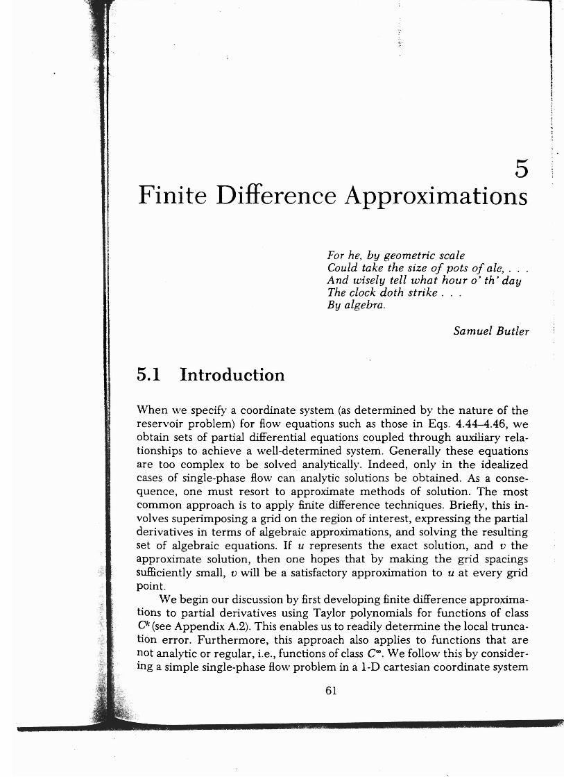
5 Finite Difference Approximations

For he, by geometric scale Could take the size of pots of ale, . And wisely tell what hour 0' th ' day The clock doth strike. By algebra.

Samuel Butler

5.1 Introduction

When we specify a coordinate system (as determined by the nature of the reservoir problem) for flow equations such as those in Eqs. 4.44-4.46, we obtain sets of partial differential equations coupled through auxiliary rela­tionships to achieve a well-determined system. Generally these equations are too complex to be solved analytically. Indeed, only in the idealized cases of single-phase flow can analytic solutions be obtained. As a conse­quence, one must resort to approximate methods of solution. The most cornmon approach is to apply finite difference techniques. Briefly, this in­volves superimposing a grid on the region of interest, expressing the partial derivatives in terms of algebraic approximations, and solving the resulting set of algebraic equations. If u represents the exact solution, and v the approximate solution, then one hopes that by making the grid spacings sufficiently small, v will be a satisfactory approximation to u at every grid point.

, We begin our discussion by first developing finite difference approxima­tions to partial derivatives using Taylor polynomials for functions of class Ck(see Appendix A.2). This enables us to readily determine the local trunca­tion error. Furthermore, this approach also applies to functions that are not analytic or regular, i.e., functions of class COD. We follow this by consider­ing a simple single-phase flow problem in a I-D cartesian coordinate system

61

, ,; ...

-::.

.

F 62 Reservoir Simulation

to illustrate several methods for solving the algebraic problem. Finally, some attention is devoted to the problems of stability and convergence.

5.2 Finite Differences TJ A

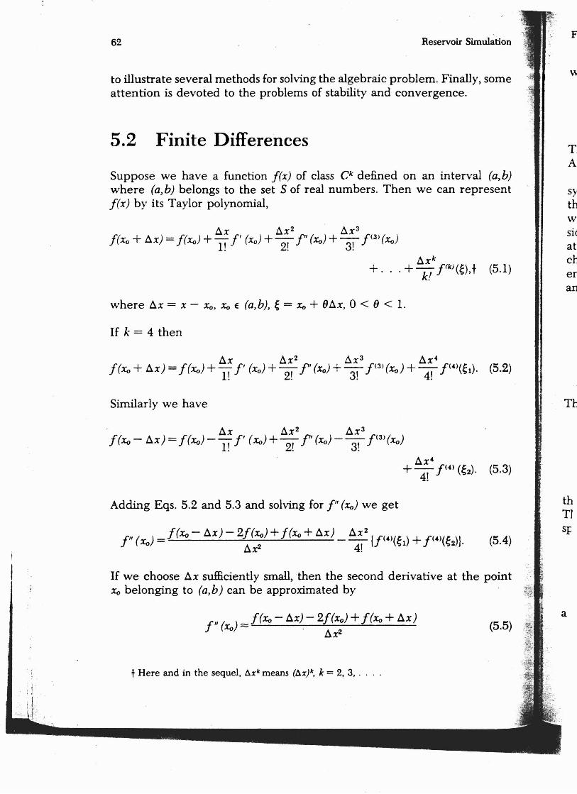
Suppose we have a function [tx) of class Ck defined on an interval (a.b) where (a,b) belongs to the set S of real numbers. Then we can represent sy fix) by its Taylor polynomial, th

w Ax Ax2 Ax3 sic

f(xo + Ax) = f(:ro) +l! f' (xo) +2! f" (:ro) +3! f ( 3 )(:ro) at chAxk

+... + k! f(k)(~),t (5.1) en an

where Ax = x - Xo, :ro E (a.b), ~ = :ro + OAx, 0 < 0 < 1.

If k = 4 then

ThSimilarly we have

thAdding Eqs. 5.2 and 5.3 and solving for f" (:ro) we get TJ

If we choose Ax sufficiently small, then the second derivative at the point :ro belonging to (a,b) can be approximated by

a

; 1, ·

f" (:ro) =::: f(:ro - AX).- 2f(xo) + f(xo + Ax) Ax2

t Here and in the sequel, tak means (ta)k, k = 2, 3, . . ..

(5.4) s1=

63 rr Simulation

.~

.•. .:lally, some 'e .

erval (a,b) represent

(; ),f (5.1)

) (;2). (5.3)

:2)\' (5.4)

at the point

(5.5)

Finite Difference Approxiinations

where the error is

This is called the local truncation error and is of O(~X2) . (See Appendix A.1 where g(x) = ~X2 and [tx) is the expression above.)

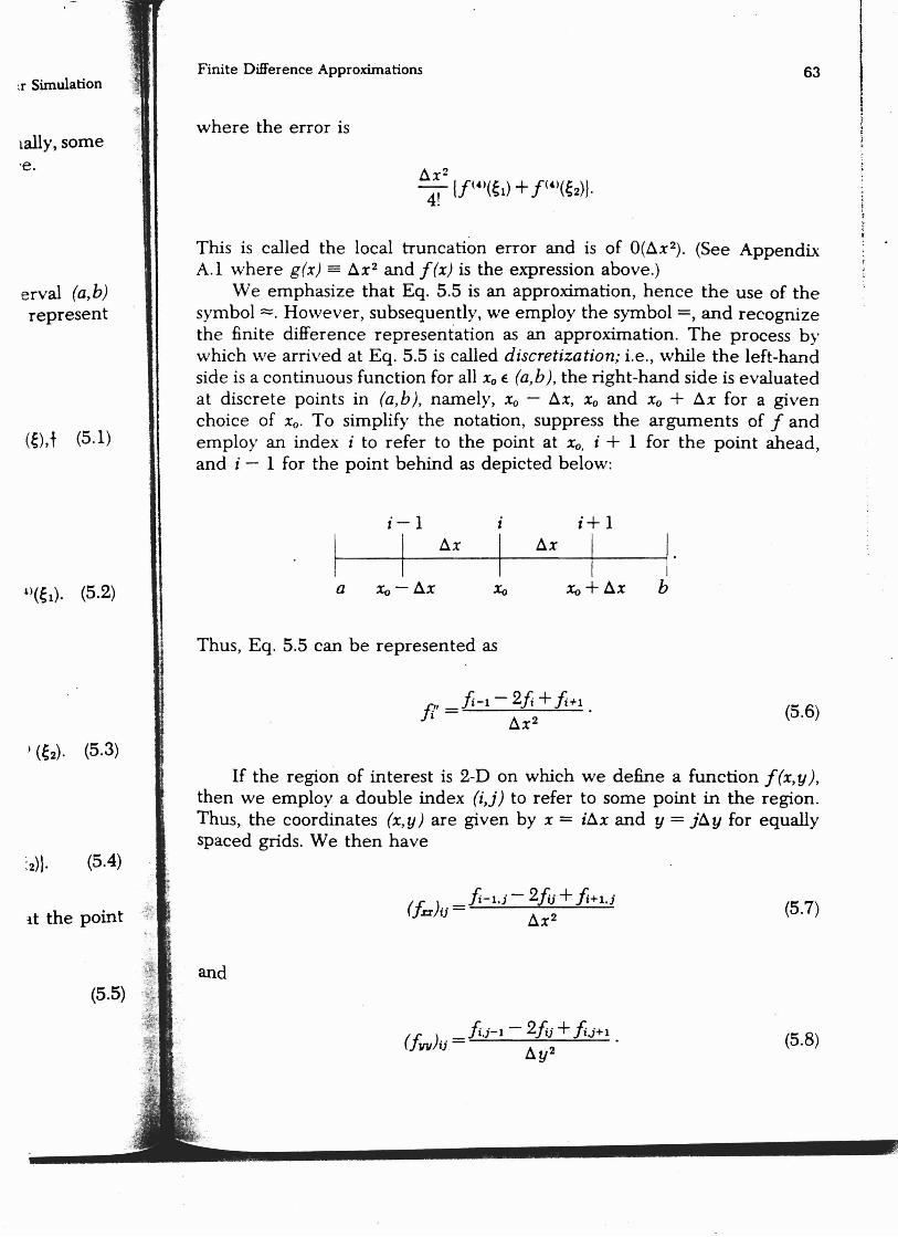
We emphasize that Eq. 5.5 is an approximation, hence the use of the symbol =. However, subsequently, we employ the symbol =, and recognize the finite difference representation as an approximation. The process by which we arrived at Eq. 5.5 is called discretization; i.e ., while the left-hand side is a continuous function for all Xo E (a.b), the right-hand side is evaluated at discrete points in (a,b), namely, Xo - S», Xo and Xo + ~x for a given choice of Xo· To simplify the notation, suppress the arguments of f and employ an index i to refer to the point at Xo. i + 1 for the point ahead, and i-I for the point behind as depicted below:

i+ 1 ~x ~x

I a Xo+~x

Thus, Eq. 5.5 can be represented as

(5.6)

If the region of interest is 2-D on which we define a function f(x,y) , then we employ a double index (i,}) to refer to some point in the region. Thus, the coordinates (x,y) are given by x = i~x and y = j~y for equally spaced grids. We then have

(5.7)

(5.8)

64 Reservoir Simulation FiJ

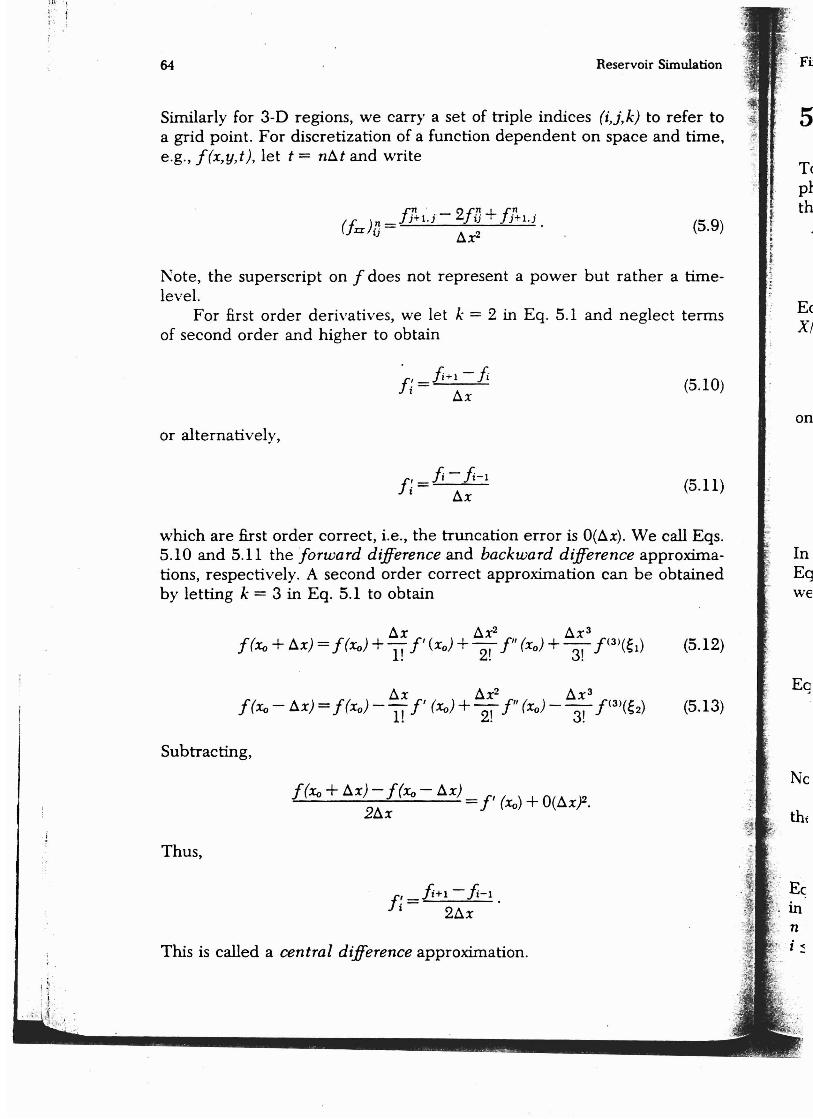
Similarly for 3-D regions, we carry a set of triple indices (i,j,k) to refer to a grid point. For discretization of a function dependent on space and time, e.g., f(x,y,t), let t = nts t and write

(5.9)

Note, the superscript on f does not represent a power but rather a time­level.

For first order derivatives, we let k = 2 in Eq. 5.1 and neglect terms of second order and higher to obtain

(5.10)

or alternatively,

(5.11)

which are first order correct, i.e., the truncation error is O(D.x). We call Eqs. 5.10 and 5.11 the forward difference and backward difference approxima­tions, respectively. A second order correct approximation can be obtained by letting k = 3 in Eq. 5.1 to obtain

(5.12)

(5.13)

Subtracting,

Thus,

This is called a central difference approximation. . .

.~ :i ~ ~

5

Tc pt th

Ec XI

on

In Eq we

Eq

Nc

ir Simulation

to refer to ~ and time,

(5.9)

ner a time­

glect terms

(5.10)

(5.11)

We call Eqs. approxima­

be obtained

(5.12)

(5.13)

-:

Finite Difference Approximations 65

5.3 Application to Single-Phase Flow

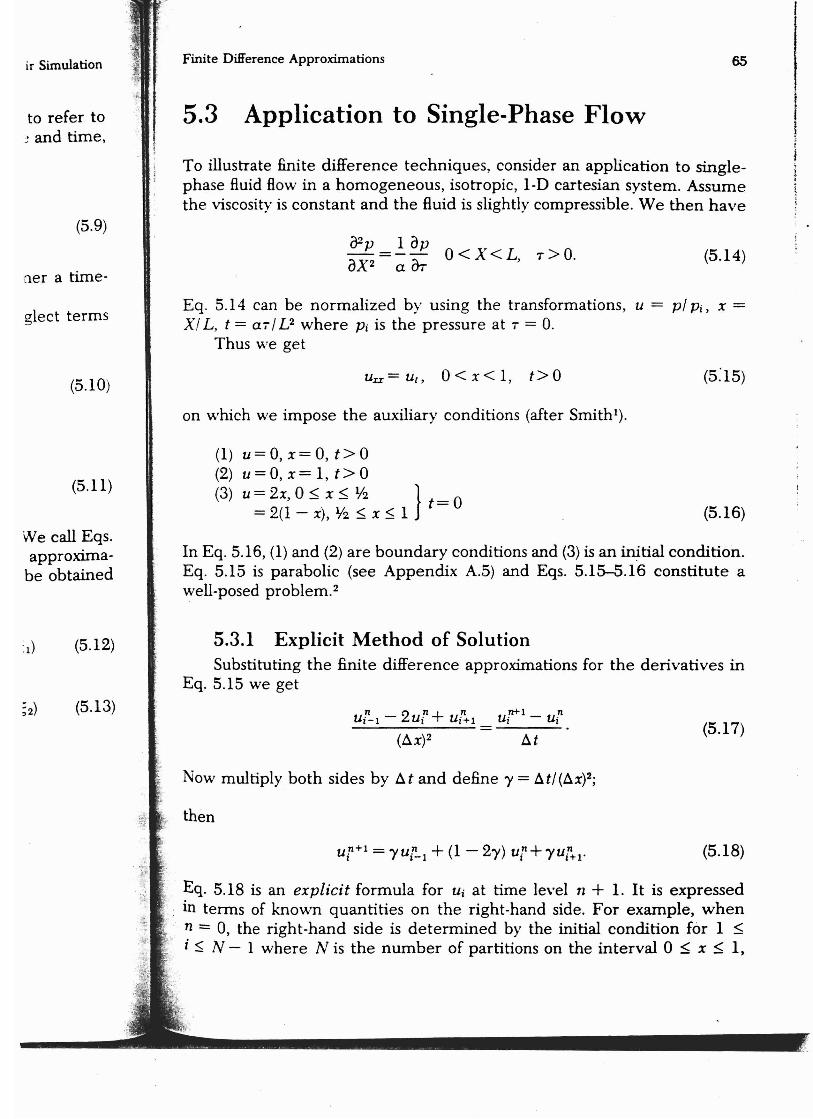
To illustrate finite difference techniques, consider an application to single­phase fluid flow in a homogeneous, isotropic, 1-D cartesian system. Assume the viscosity is constant and the fluid is slightly compressible. We then have

02p=.!.ap O<X<L 0 (5.14)aX2 a OT ' T> .

Eq. 5.14 can be normalized by using the transformations, u = pi Pi, X = X IL , t = aTI L2 where Pi is the pressure at T = O.

Thus we get

Uxx = u. , 0 < x < 1, t> 0

on which we impose the auxiliary conditions (after Smith').

(1) u=O,x=O,t>O (2) U = 0, x= 1, t> 0 (3) U = 2x, 0 ~ x s lf2 } t = 0

= 2(1 - x), lf2 ~ X ~ 1 (5.16)

In Eq. 5.16, (1) and (2) are boundary conditions and (3) is an initial condition. Eq. 5.15 is parabolic (see Appendix A .5) and Eqs . 5.15--5.16 constitute a well-posed problem."

5.3.1 Explicit Method of Solution Substituting the finite difference approximations for the derivatives in

Eq. 5.15 we get

(5.17)

Now multiply both sides by t1t and define y = t1tl(t1x)2;

(5.18)

Eq. 5.18 is an explicit formula for u, at time level n + 1. It is expressed ; : in terms of known quantities on the right-hand side. For example, when ,: .' n = 0, the right-hand side is determined by the initial condition for 1 ~

i S N - 1 where N is the number of partitions on the interval 0 ~ x ~ 1,

.t\. ' ,

Reservoir Simulation :. 66

i.e., Ax = 11 N. The values of u at i = 0 and i = 1 are given by the boundary conditions. Notice we have the following computational star:

i-1 i #+1 n: • • •

1 n+ 1: •

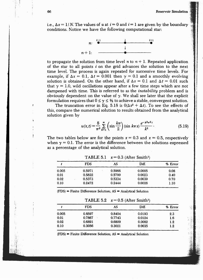
to propagate the solution from time level n to n + 1. Repeated application of the star to all points i on the grid advances the solution to the next time level. The process is again repeated for successive time levels. For example, if Ax = 0.1, At = 0.001 then y = 0.1 and a smoothly evolving solution is obtained. On the other hand, if Ax = 0.1 and At = 0.01 such that y = 1.0, wild oscillations appear after a few time steps which are not dampened with time. This is referred to as the instability problem and is obviously dependent on the value of y. We shall see later that the explicit formulation requires that 0 ~ y ~ ¥2 to achieve a stable, convergent solution.

The truncation error in Eq. 5.18 is O(Ax2 + At). To see the effects of this, compare the numerical solution to results obtained from the analytical solution given by

2 28 (lcrr) e: k 1T I u (x, t) =- LCIl

sin -2 (sin hrx) k . (5.19) ~2~1 2

The two tables below are for the points x = 0.3 and x = 0.5, respectively when y = 0.1. The error is the difference between the solutions expressed as a percentage of the analytical solution.

TABLE 5.1 x = 0.3 (After Smith-)

t FDS AS Diff. % Error

0.005 0.5971 0.5966 0.0005 0.08 0.01 0.5822 0.5799 0.0023 0.40 0.02 0.5373 0.5334 0.0039 0.70 0.10 0.2472 0.2444 0.0028 1.10

. ;

(FDS) = Finite Difference Solution; AS == Analytical Solution

TABLE 5.2 x=0.5 (After Smith')

t FDS AS Diff. % Error - . .,

0.005 0.8597 0.8404 0.0193 2.3 0.01 0.02 0.10

0.7867 0.6891 0.3056

0.7743 0.6809 0.3021

0.0124 0.0082 0.0035

1.6 1.2 1.2

;. .:'!­.£ ,.:.

(FDS) ... Finite Difference Solution; AS E Analytical Solution

Simulation

boundary

pplication the next

evels. For .' evolving 0.01 such

ch are not .ern and is he explicit rt solution. ~ effects of ~ analytical

(5.19)

espectively s expressed

70 Error

0.08 0.40 0.70 1.10

% Error

2.3 1.6 1.2 1.2

Finite Difference Approximations 67

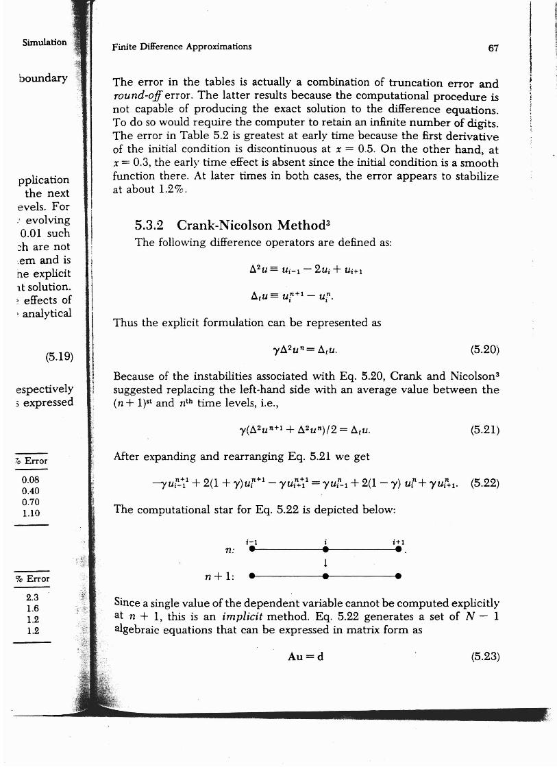
The error in the tables is actually a combination of truncation error and round-off error. The latter results because the computational procedure is not capable of producing the exact solution to the difference equations. To do so would require the computer to retain an infinite number of digits. The error in Table 5.2 is greatest at early time because the first derivative of the initial condition is discontinuous at x = 0.5. On the other hand, at x = 0.3, the early time_effect is absent since the initial condition is a smooth function there. At later times in both cases, the error appears to stabilize at about 1.2o/c.

5.3.2 Crank-Nicolson Method" The following difference operators are defined as:

Atu =U!1+1 - ul' , l l

Thus the explicit formulation can be represented as

(5.20)

II

Because of the instabilities associated with Eq. 5.20, Crank and Nicolson" i suggested replacing the left-hand side with an average value between theI

(n + 1)st and nth time levels, i.e.,

(5.21)

After expanding and rearranging Eq. 5.21 we get

n+l + 2(1 + ) n+l n+l - n + 2(1 - Y ) n+ YUi+l. (5.22),Uj-l y u i - YUi+l - YUi-l u; n

The computational star for Eq. 5.22 is depicted below:

i-I i HI n: • • • •

1 n+ 1: • ••

Since a single value of the dependent variable cannot be computed explicitly at n + 1, this is an implicit method. Eq. 5.22 generates a set of N - 1 algebraic equations that can be expressed in matrix form as

Au=d (5.23)

.."

68

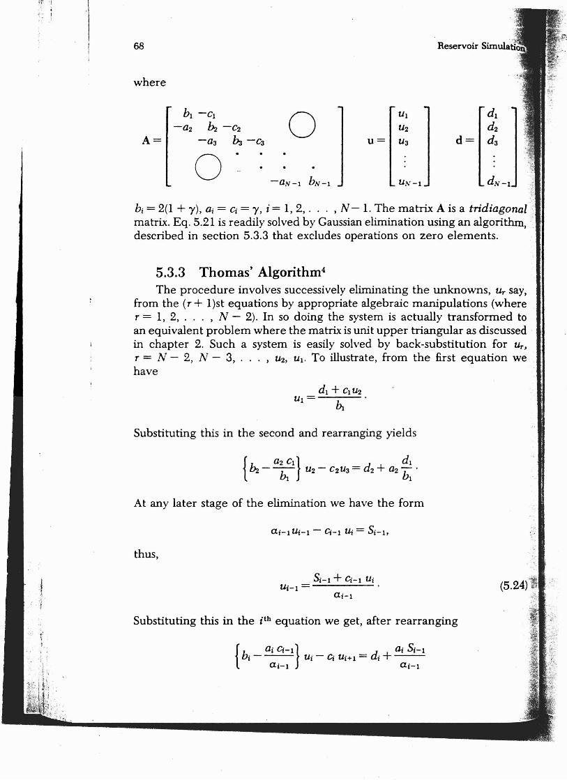
where

hI -CI

-a2 ll2 -C2 oA = -a3 b:J -C3

o hi = 2(1 + 'Y), a, = Ci = 'Y, i = 1,2, . . . , N ­matrix. Eq. 5.21 is readily solved by Gaussian elimination using an algorithm, described in section 5.3.3 that excludes operations on zero elements.

5.3.3 Thomas' Algorithm" The procedure involves successively eliminating the unknowns, Ur say,

from the (r + l)st equations by appropriate algebraic manipulations (where r = 1, 2, ... , N - 2). In so doing the system is actually transformed to an equivalent problem where the matrix is unit upper triangular as discussed in chapter 2. Such a system is easily solved by back-substitution for !Jr.,

r = N - 2, N - 3, . . . , U2, UI. To illustrate, from the first equation we have

1. The matrix A is a tridiagonal

Substituting this in the second and rearranging yields

At any later stage of the elimination we have the form

thus,

~-I + Ci-I Ui Uj-I =

Substituting this in the i th equation we get, after rearranging

I

j

irnulation -'­

d1

d2

d3

diagonal gorithm, rts.

1S, Ur say, IS (where orrned to discussed n for Ur,

ration we

Finite Difference Approximations 69

where

a, Ci-l uj=bj - - - (5.25)

aj-l

!.­

~ _ d aj Sj-l - - j+ (5.26)

Uj-l I I -

and 1

(5.27)

Eqs. 5.25-5.26 are forward recurrence formulas that can be used to generate the a- and Sarrays using Eq. 5.27 for starting values. Once these arrays are obtained, the backward recursion formula, Eq . 5.24, is used to compute :'.t­

i . '

Uj-l, i = N, N -1 , N - 2, . . . , 1 subject to the constraint, CN-l = O. This technique is known as the Thomas algorithm for tridiagonal matrices.' Simi­lar algorithms have been presented by others.s" however, they are not as efficient as Thomas' algorithm, though less round-off error may be incurred.s Where applicable, the Thomas algorithm is used almost exclusively in reser­voir simulation problems.

5.4 Stability Analysis

"

.1 :-,

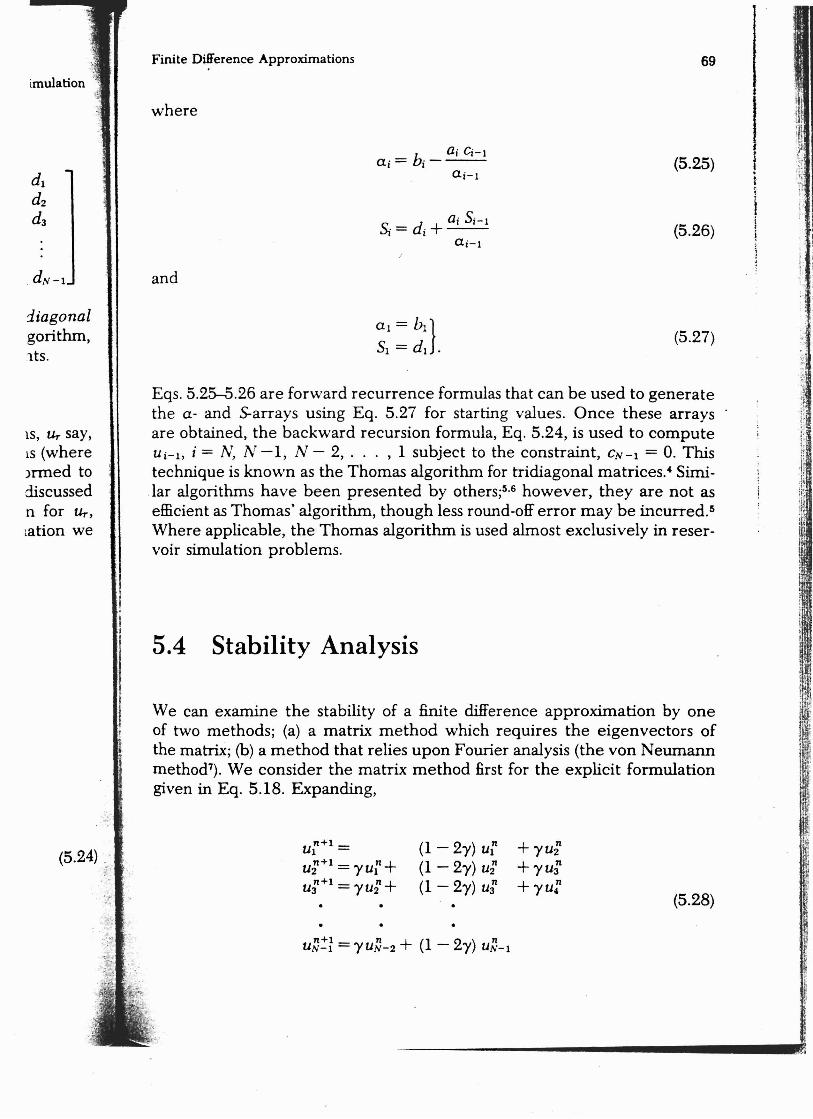
We can examine the stability of a finite difference approximation by one of two methods; (a) a matrix method which requires the eigenvectors of the matrix; (b) a method that relies upon Fourier analysis (the von Neumann method"). We consider the matrix method first for the explicit formulation given in Eq. 5.18. Expanding,

(1 - 2')') uf(5.24) _.­(1 - 2')') u;. ::... :

n(1 - 2')') U3(5.28)

n+l - n + (1 2) nUN-l - ')'UN-2 - ')' UN-l

. ;'.-,-_..''r .'.-­ ....~-- -~..... ,....;'..-----.- ._._..

Reservoir Simulation']70

0 n 1ur+

1 (1 - 2y) y Ul

u:+y (1 - 2')') ')' u:

(5.29) ; :~.o -. 1 0;

n+l -:')' (1 - 2')') U~-l UN-l

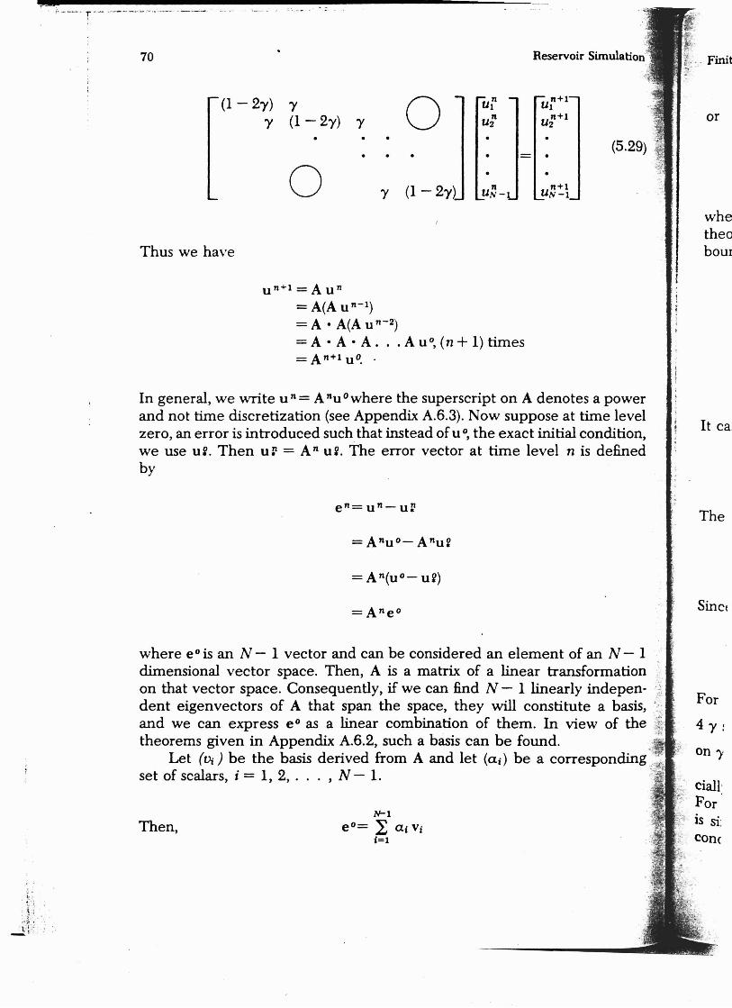
Thus we have

u n +1 = A u " = A(A un-I) = A • A(A u n-2) = A • A • A. . . A u 0, (n + 1) times = An+l u O••

In general, we write u n= Anuowhere the superscript on A denotes a power and not time discretization (see Appendix A.6.3). Now suppose at time level zero, an error is introduced such that instead of u 0, the exact initial condition, we use u s. Then u~ = An u s. The error vector at time level n is defined by

en=un-u~

= Anuo- Anu~

= An(uo- us)

where eO is an N - 1 vector and can be considered an element of an N - 1 dimensional vector space. Then, A is a matrix of a linear transformation on that vector space. Consequently, if we can find N - 1 linearly indepen- - ~_

dent eigenvectors of A that span the space, they will constitute a basis, .. and we can express eO as a linear combination of them. In view of the ii~ theorems given in Appendix A.6.2, such a basis can be found.

Let (Vj) be the basis derived from A and let (at) be a correspondingset of scalars, i = 1, 2, ... , N - 1.

lrl

Then, eO= I ai Vi 1=1

whe theo bour

It ca:

The

Sine.

For

on .,

ciall­For is si:

:; cone

' _' ~. ;ii

Simulation

(5.29)

s a power :ime level xmdition, is defined

~ an N-l .Formation " indepen­te a basis, ew of the

-esponding , :

Finite Difference Approximations 71

N-l

or e"= L ai A""i t=1

N-l

= L ai ArVi (5.30) i=1

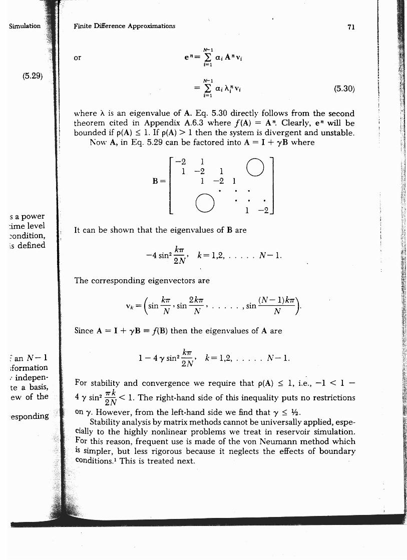
where A is an eigenvalue of A. Eq. 5.30 directly follows from the second theorem cited in Appendix A.6.3 where f(A) = A". Clearly, e " will be bounded if p(A) ::; 1. If p(A) > 1 then the system is divergent and unstable.

Now A, in Eq. 5.29 can be factored into A = I + ')'B where L :.t \ ,

-2 1 01 -2 1 B= 1 -2 1

0 1 -2

It can be shown that the eigenvalues of Bare

kst-4 S1'n2 -, k - 1 2 N - 12N -, , . , , , , .

The corresponding eigenvectors are

, . ktt , 2krr , (N - l)krr) Vk = ( SInN ' SIn N' . . , , . ,sIn N '

Since A = I + ')'B == f(B) then the eigenvalues of A are

krr 1 - 4 ')' S1'n 2 -, k - 1 2 11. T- 12N -"" ,.,1'1 ,

For stability and convergence we require that p(A) ::; 1, i.e. -1 < 1 ­

4 'Y sin- ;~ < 1. The right-hand side of this inequality puts no restrictions

on 'Y. However, from the left-hand side we find that')' ::; 112, Stability analysis by matrix methods cannot be universally applied, espe­ 1:

cially to the highly nonlinear problems we treat in reservoir simulation, For this reason, frequent use is made of the von Neumann method which is simpler, but less rigorous because it neglects the effects of boundary conditions,l This is treated next.

'

72

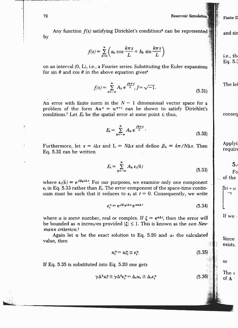
Any function f(x) satisfying Dirichlet's conditions- can be represented by

oc ( ktt x k7rX)f(x) = k~O ak cos L + bk sin L

'

on an interval (0, L), i.e., a Fourier series. Substituting the Euler expansions for sin () and cos 8in the above equation gives"

oc Jkrr I

f(x) = L Ak e-L-, ] = FL k=-oc (5.31)

An error with finite norm in the N - 1 dimensional vector space for a problem of the form Au n = U n+1 can be shown to satisfy Dirichlet's conditions." Let E; be the spatial error at some point i; thus,

OC Jkrr I e= I Ake-L- . k=-oc (5.32)

Furthermore, let x = its» and L = N!:1x and define 13k = k7T /N!:1x. Then Eq. 5.32 can be written

Ei> L oc

Ak€dk) k=-oc (5.33)

J f3k it.I.where €dk) = e For our purposes, we examine only one component €i in Eq. 5.33 rather than e. The error component of the space-time contin­uum must be such that it reduces to €i at t = O. Consequently, we write

€!l = eJf3 k i A I e naA t (5.34)I

where a is some: number, real or complex. If t = ea A t , then the error will be bounded as n increases provided ItI ~ 1. This is known as the von Neu­mann criterion.i

Again let u be the exact solution to Eq. 5.20 and a. the calculated value, then

(5.35) .

If Eq. 5.35 is substituted into Eq. 5.20 one gets or

The E

of A

Finite D

and sin

i.e., thr Eq.5.3

The lef

conseq

Applyii require

5.~

Fa of the

If we,

Since exists.

'

• • ••

:~

esented ]

oansions

(5.31)

.ce for a irichlet's

(5.32)

~x. Then

(5.33)

imponent .ie contin­we write

(5.34)

error will ~ von Neu-.

calculated

or

(5.35) :;: - i': . ~

consequently, ,

.~

. . ,

,. . ~

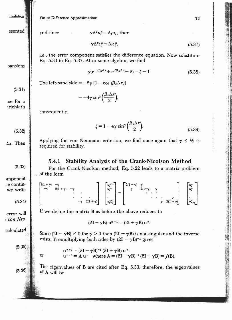
Applying the von Neumann criterion, we find once again that y required for stability.

5.4.1 Stability Analysis of the Crank-Nicolson Method For the Crank-Nicolson method, Eq. 5.22 leads to

of the form

2(1 +'Y) , ] U~ + l] [2(1 - 'Y) 'YU;+l 'Y 2(1,) 'Y , 2(1 ~'Y) -: : • . = . . .

[ [, 2(1 +'Y) u~:: 'Y

If we define the matrix B as before the above reduces to

(21 - yB) u n +1 = (21 + yB) u ",

t Since 121 - yBi ¥: 0 for y > 0 then (21 ­exists. Premultiplying both sides by (21 - yB)-l gives

U n+1 = (21 - yB)-l (21+ yB) u " u n+1 = A u " where A = (21 - yB)-l (21+ yB) =

The eigenvalues of B are cited after Eq. 5.30; therefore, the eigenvalues of A will be

I Finite Difference Approximations 73

and since

(5.37)

i.e., the error component satisfies the difference equation. Now substitute Eq. 5.34 in Eq. 5.37. After some algebra, we find

(5.38)

The left-hand side = -2y [1 - cos (,Bk~X)]

(5.39)

]

'Y

2(1 - 'Y)

f(B) .

yB) is nonsingular and the inverse

a matrix problem

$ 112 is

& ,

Reservoir Simulation 74

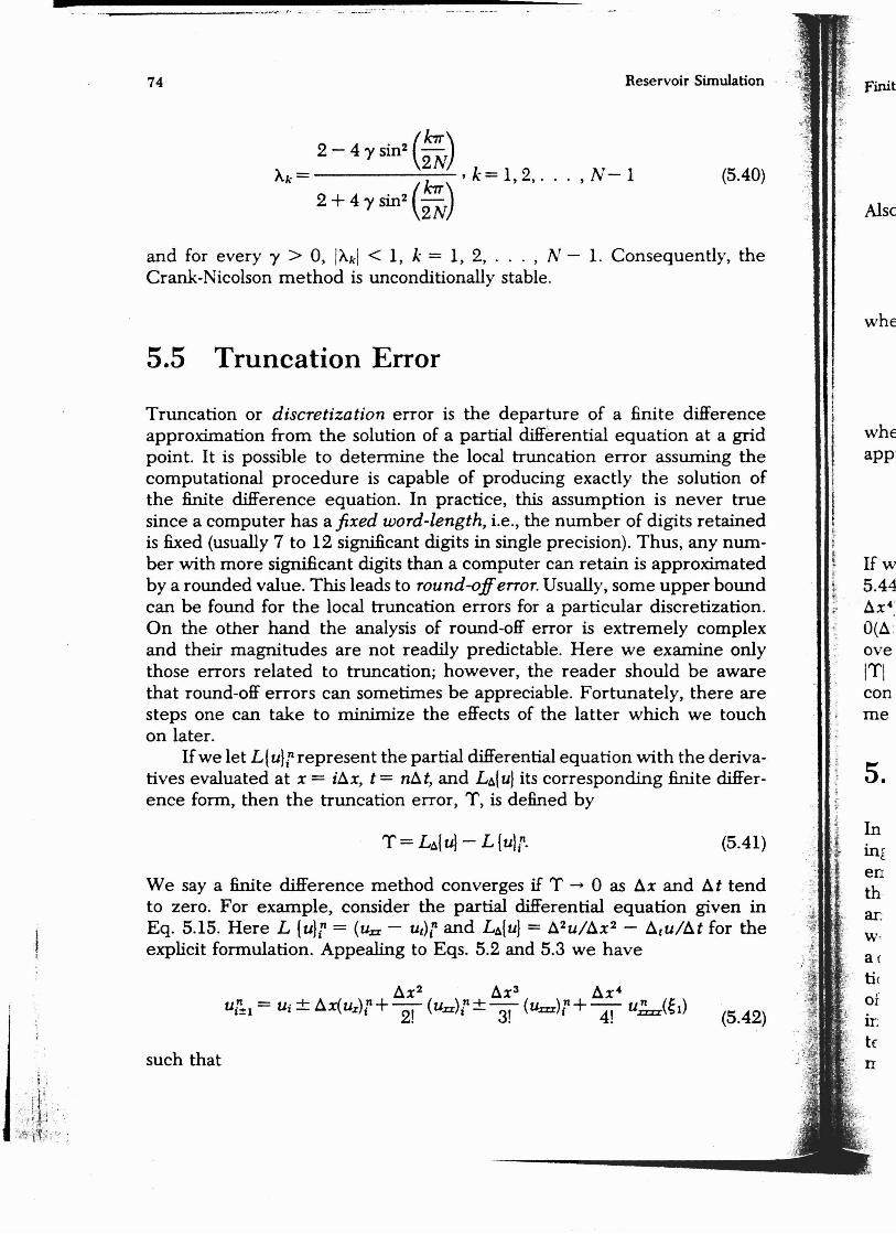
2 - 4 y sin! (~) Ak = /crr «]: = 1, 2,. . . ,N - 1 (5.40)

2+4 YSin2(2N)

and for every Y > 0, IAkl < 1, k = 1, 2, .. . , N ­Crank-Nicolson method is unconditionally stable.

5.5 Truncation Error

1. Consequently, the

Truncation or discretization error is the departure of a finite difference approximation from the solution of a partial differential equation at a grid point. It is possible to determine the local truncation error assuming the computational procedure is capable of producing exactly the solution of the finite difference equation. In practice, this assumption is never true since a computer has a fixed word-length, i.e ., the number of digits retained is fixed (usually 7 to 12 significant digits in single precision). Thus, any num­ber with more significant digits than a computer can retain is approximated by a rounded value. This leads to round-offerror. Usually, some upper bound can be found for the local truncation errors for a particular discretization. On the other hand the analysis of round-off error is extremely complex and their magnitudes are not readily predictable. Here we examine only those errors related to truncation; however, the reader should be aware that round-off errors can sometimes be appreciable. Fortunately, there are steps one can take to minimize the effects of the latter which we touch on later.

Ifwe let Ll u}r represent the partial differential equation with the deriva­tives evaluated at x = i6.x, t = ntxt, and Lt.lu} its corresponding finite differ­ence form, then the truncation error, 1', is defined by

T = Lt.l u} - L Iu} r- (5.41)

We say a finite difference method converges if T - 0 as 6.x and 6.t tend to zero. For example, consider the partial differential equation given in

"

Eq. 5.15. Here L {u}r = (Urc - ut)f and Lt.lu} = A2ul 6.x 2 - Atul 6.t for theI explicit formulation. Appealing to Eqs. 5.2 and 5.3 we haveI

(5.42)

such that

Also

whe

I ! i

whe

I appi

I r r

t Ifw I

i 5.44" f. .. 6.x" 0(6. : ove 11'1 con me

5. I .­J

~ In .f t in t

en : . th

ar w; a( ti t of if: tE

lation

3.40)

. the

ence grid

-y the::>

)n of true

lined num­.iated -ound ation. nplex only

[ware 'e are touch

eriva­iiffer­

(5.41)

' tend en in .....,

)r the

(5.42)

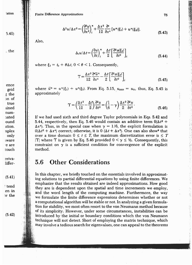
Finite Difference Approximations 75

(5.43)

Also,

'.

(5.44)

where ~3 = to + 86.t, 0 < 8 < 1. Consequently,

(5.45)

where un = Un(~l) + Un(~2)' From Eq. 5.15, \ u= = Utt, thus, Eq. 5.45 is

approximately

1" = (6.X2

_ 6.t) (}2u = (~_ ) 6.x2

(}2u . 12 2 3t2 6 v 2 3t 2 (5.46)

If we had used sixth and third degree Taylor polynomials in Eqs. 5.42 and 5.44, respectively, then Eq. 5.46 would contain an additive term 0(~t2 + ~X4). Thus, in the special case when y = 1/6, the explicit formulation is O(~ t 2 + ~X4) correct; otherwise, it is 0 (~t + ~X2). One can also show? that over a time domain 0 ~ . t ~ T, the maximum discretization error is ~ T 11"1where 1" is given by Eq. 5.46 provided 0 < y ~ Y2. Consequently, this constraint on y is a sufficient condition for convergence of the explicit method.

, :;

5.6 Other Considerations

In this chapter, we briefly touched on the essentials involved in approximat­,

i ing solutions to partial differential equations by using finite differences. We i emphasize that the results obtained are indeed approximations. How goodt• they are is dependent upon the spatial and time increments we employ,

t and the word length of the computing machine. Furthermore, the way we formulate the finite difference expressions determines whether or not a computational algorithm will be stable or not. In analyzing a given formula­tion for stability, we most often resort to the von Neumann method because of its simplicity. However, under some circumstances, instabilities can be introduced by the initial or boundary conditions which the von Neumann technique will not detect. Short of employing the matrix technique, which may involve a tedious search for eigenvalues, one can appeal to the theorems

;

e ,

, .

I

J

j

-

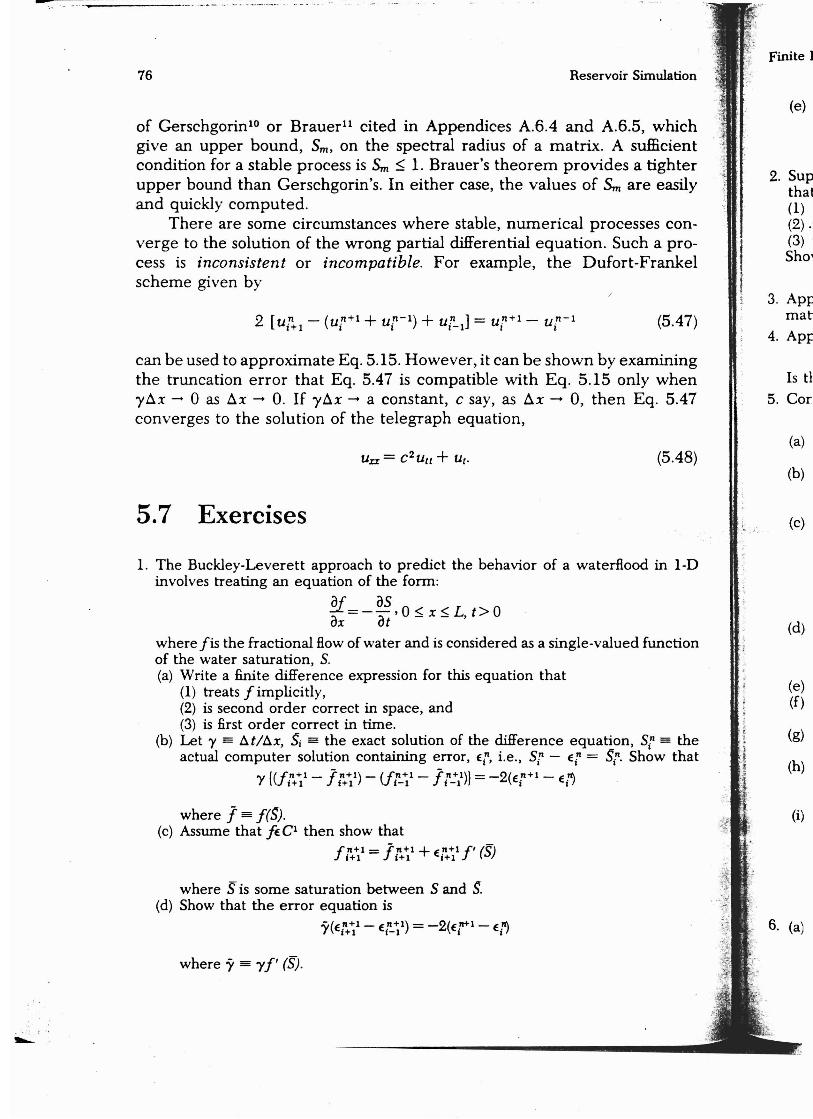
76 Reservoir Simulation

of Cerschgorint? or Brauer!' cited in Appendices A.6.4 and A.6.5, which :~

give an upper bound, Sm, on the spectral radius of a matrix. A sufficient . ~

condition for a stable process is S« :S 1. Brauer's theorem provides a tighter upper bound than Cerschgorin's. In either case, the values of Sm are easily and quickly computed.

There are some circumstances where stable, numerical processes con­verge to the solution of the wrong partial differential equation. Such a pro­cess is inconsistent or incompatible. For example, the Dufort-Frankel scheme given by

(5.47)

can be used to approximate Eq. 5.15. However, it can be shown by examining the truncation error that Eq. 5.47 is compatible with Eq. 5.15 only when "lAx -- 0 as Ax -- 0. If "lAx -- a constant, c say, as Ax -+ 0, then Eq. 5.47 converges to the solution of the telegraph equation,

Uu = c2u., + u.. (5.48)

5.7 Exercises

1. The Buckley-Leverett approach to predict the behavior of a waterflood in 1-D involves treating an equation of the form:

a+ as&= - at ' 0 ~ x ~ L, t> 0

where fis the fractional Howof water and is considered as a single-valued function of the water saturation, S. (a) Write a finite difference expression for this equation that

(1) treats f implicitly, (2) is second order correct in space, and (3) is first order correct in time.

(b) Let "/ == At/Ax, ~ = the exact solution of the difference equation, Sr == the actual computer solution containing error, £t, i.e., Sr - q = Sr. Show that

"'I /(fn + l - f- !,+1) - (fn+l - r !'+1)! = -2(e!l+1 - e!flHI 1+1 j-l 1-1 1 i !

where 1 == f(S). (c) Assume that ftC I then show that

f n + l = f- n+l + en +1 f ' (5)1+1 1+1 1+1

where Sis some saturation between Sand S. (d) Show that the error equation is

- (e!l+1 - e!,+I) = -2(e~1 - e!fl"/ 1+1 1-1 I i !

where 'Y == "'If' (S).

Finite I

(e)

2. Sup that (1) (2) .

(3) Shoi

3. APt: mat

4. API:

Is tl

5. Cor

(a)

(b)

(c)

(d)

(e) (f)

(g)

J .!; (h)

(i)

6. (a)

;j

iulation

which Bcient cighter . easily

es con­a pro­rankel

(5.47)

mining . when ::}. 5.47

(5.48)

i in I-D

function

S» == theI

l OW that

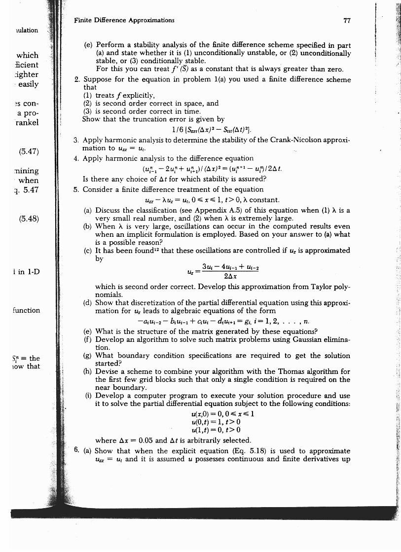
'I Finite Difference Approximations 77

(e) Perform a stability analysis of the finite difference scheme specified in part (a) and state whether it is (I) unconditionally unstable, or (2) unconditionally stable. or (3) conditionally stable. . For this you can treat f' (5) as a constant that is always greater than zero.

2. Suppose for the equation in problem L(a) you used a finite difference scheme that

' j (I) treats f explicitly, ,,(2) is second order correct in space, and (3) is second order correct in time. Show that the truncation error is given by

1I61~d~x)2 - Sttd~t)21 .

3. Apply harmonic analysis to determine the stability of the Crank-Nicolson approxi­mation to Un = Ur.

4. Apply harmonic analysis to the difference equation

( U n - 2u n + u" )/ (ts») 2 = (U!,+l - u .m/2~t. :1-1 I 1+1 I j I ,

Is there any choice of ~t for which stability is assured?

5. Consider a finite difference treatment of the equation -. ~

Uxr - AUr = Ur, 0::0::;; x::O::;; 1, t> 0, Aconstant.

(a) Discuss the classification (see Appendix A.5) of this equation when (1) A is a very small real number, and (2) when A is extremely large.

(b) When A is very large, oscillations can occur in the computed results even when an implicit formulation is employed. Based on your answer to (a) what is a possible reason?

(c) It has been found-s that these oscillations are controlled if Ux is approximated by

3u; - 4Ui-l + U;-2 o-> 2~x

which is second order correct. Develop this approximation from Taylor poly­nomials.

(d) Show that discretization of the partial differential equation using this approxi­mation for Ur leads to algebraic equations of the form

-lliUi -2 - ~Ui-l + CiUj - c:4Ui+l = gi. i = 1,2, ... , n. (e) What is the structure of the matrix generated by these equations? (f) Develop an algorithm to solve such matrix problems using Gaussian elimina­

tion. (g) What boundary condition specifications are required to get the solution · i

started? . ;

(h) Devise a scheme to combine your algorithm with the Thomas algorithm for the .first few grid blocks such that only a single condition is required on the near boundary. .,.

~ . '(i) Develop a computer program to execute your solution procedure and use !~~

it to solve the partial differential equation subject to the following conditions:

u(x,O) = 0, °::0::;; x::O::;; 1 u(O,t) = 1, t> ° u(l,t) = 0, t> °

where ~x = 0.05 and ~t is arbitrarily selected.

6. (a) Show that when the explicit equation (Eq. 5.18) is used to approximate Uxr = u, and it is assumed U possesses continuous and finite derivatives up

,\i;

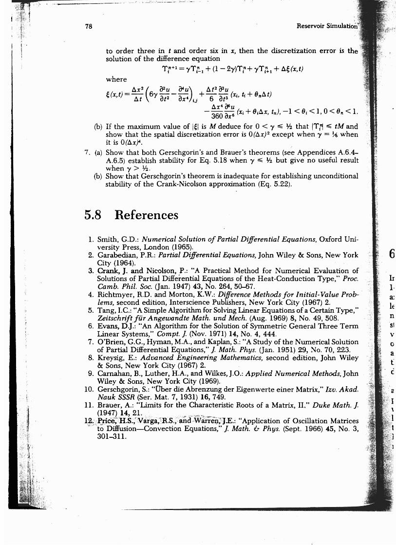
Reservoir Simulatio~'~'

to order three in t and order six in z, then the discretization error is the C'

solution of the difference equation Tn+1 = '\IT.n + (1 - 2'\1)Tn+ '\ITn + AI:. (x t)

I I I-I I I I i+ 1 r",

where

At2(}3uAX 2 ( OZu (}4u)

Hx,t) = At 6"1 ot2 - Ox' lj +6 ot3 (Xi, it+ 8nAt) Ax'i)6u

- 360 ox6 (x,+ 8 jAx, t-), -1 < e, < I, 0 < e; < 1.

(b) If the maximum value of I~ I is M deduce for 0 < "I ~ Y2 that ITi~ ~ tM and show that the spatial discretization error is 0(AX)2 except when "I = ~ when it is o(Axf.

/

7. (a) Show that both Cerschgorin's and Brauer's theorems (see Appendices A.6.4­A.6.5) establish stability for Eq. 5.18 when "I ~ lf2 but give no useful result when "I > lf2 .

(b) Show that Cerschgorin's theorem is inadequate for establishing unconditional stability of the Crank-Nicolson approximation (Eq. 5.22) .

5.8 References

1. Smith, G.D.: Numerical Solution of Partial Differential Equations, Oxford Uni­versity Press, London (1965).

2. Garabedian, P.R.: Partial Differential Equations, John Wiley & Sons, New York 6 City (1964).

3. Crank, J.and Nicolson, P.: "A Practical Method for Numerical Evaluation of Solutions of Partial Differential Equations of the Heat-Conduction Type," Proc. II Camb. Phil. Soc. (Jan. 1947) 43, No. 264,50-07. ,,' 1·

4. Richtmyer, R.D. and Morton, K.W.: Difference Methods for Initial- Value Prob- . 3J lems, second edition, Interscience Publishers, New York City (1967) 2. IE5. Tang, I.e.: "A Simple Algorithm for Solving Linear Equations of a Certain Type," Zeitschriftfiir Angewandte Math. und Mech. (Aug. 1969) 8, No. 49,508. n

6. Evans, D.].: "An Algorithm for the Solution of Symmetric General Three Term 51 Linear Systems," Compt.]. (Nov. 1971) 14, No.4, 444 . v

7. O'Brien, G.G., Hyman, M.A., and Kaplan, S.: "A Study of the Numerical Solution of Partial Differential Equations," ]. Math. Phys. (Jan. 1951) 29, No. 70, 223.

8. Kreysig, E.: Advanced Engineering Mathematics, second edition, John Wiley & Sons, New York City (1967) 2.

9. Carnahan, B., Luther, H.A., and Wilkes, J.D.: Applied Numerical Methods, John Wiley & Sons, New York City (1969).

10. Gerschgorin, S.: "Uber die Abrenzung der Eigenwerte einer Matrix," Izo . Akad. Nauk SSSR (Ser. Mat. 7, 1931) 16, 749.

11. Brauer, A.: "Limits for the Characteristic Roots of a Matrix, It" Duke Math . ]. (1947)14,21. , .: ,.. ..-'. .. _

1¥;£IFce;:H.S.~":varga;::R.S. ,: : ai'id-w arrei:i;'J £ .: "Application of Oscillation Matrices to Diffusion-Convection Equations," ]. Math. & Phys. (Sept. 1966) 45, No.3, 301-311.