The Fading Memory Polynomial Velocity StrategyCME/Globex from January 3, 2008 to January 8, 2016....

Copyright 2016 Dennis Meyers nthOrderFadmV-EC1m Page-1

Trading 1Min Bar Euro Futures Using The Fading Memory Polynomial Velocity Strategy

Jan/2008 –Jan/2016 Working Paper January 2016

Copyright 2016 Dennis Meyers This is a mathematical technique that fits a nth order polynomial to the last T price bars but calculates the coefficients of the polynomial such that the error between the current nth order polynomial and the current bar is weighted much higher than the error between the price T bars ago and the value of the nth order polynomial T bars ago. As an example, if the latest price is at time t and the price made a turn at time bar t-10, then we do not want prices prior to t-10 affecting the current polynomial fit as much. As will be shown the most familiar case of this fading memory technique is the exponential moving average. The fading memory technique is in contrast to the Least Squares Polynomial fit, which weights all past errors between the polynomial and the price bar equally. In previous working papers at http://www.meyersanalytics.com/papers.php we showed how the application of a price curve generated by Nth Order Fixed Memory Polynomial Velocity could be used to develop a strategy to buy and sell futures intraday. The reasoning behind this type of system was to only trade when the price trend velocity was above a certain threshold. Many times prices meander around without any notable trend and this is considered noise. During these times we do not wish to trade because of the cost of whipsaw losses that would occur from this type of price action. When a price trend finally starts, the velocity of that price trend moves above a minimum threshold noise value. Thus the velocity system would only issue a trade when certain velocity thresholds above “noise” levels are crossed. The velocity system that we will use here to trade the Euro futures contract is called the Nth Order Fading Memory Adaptive Polynomial Velocity Strategy. The word “Adaptive” is used because the polynomial inputs change over time, adapting to the changing trading patterns of the Euro futures contract. The Nth Order Fading memory Adaptive Polynomial Velocity Strategy has a number of unknown inputs that we have to determine before we can use this strategy to trade. These unknown inputs to the Fading Memory Polynomial are the polynomial order, the optimum number of prices we need to determine the coefficients of the polynomial and finally the velocity thresholds. Here we will use Walk Forward Optimization and out-of-sample performance to determine the “best” polynomial inputs as well as how these inputs should change over time. We will use the nth Order Fading Memory Adaptive Polynomial Velocity System to trade the Euro futures contract on an intraday basis using one minute bar price data. To test this strategy we will use one minute bar prices of the Euro futures contract(EC) traded on the CME/Globex from January 3, 2008 to January 8, 2016. The nth Order Fading Memory Adaptive Polynomial Velocity Defined The adaptive nth order Fading Memory Polynomial Velocity is constructed and plotted at each bar by solving for the coefficients b1, b2, b3, …bn for the discrete orthogonal Meixner polynomials at each bar using the exponential decay factor α=(1-β) and the equation for bj shown in the “Math” appendix of this paper. Then Velocity(T+1) is constructed from the equation shown in the “Math” appendix and plotted under the price chart. The velocity of a 2nd, 3rd and 4th order polynomial should change faster than the straight line ( 1st order velocity). As observed from the 2nd order velocity equation in the “Math” section, there is an acceleration component in the calculation of the velocity. This means that the 2nd order velocity will reflect a change in the price trend much faster than the straight line velocity which does not have an acceleration component. The same is true for 3rd and 4th order velocities. Whether higher order polynomial velocities is an advantage or not we will let the computer decide when we let the computer search for the “best” polynomial degree as described below. At each bar we calculate the nth order (1st through 4th ) fading memory polynomial velocity from the formulas in the “Math” appendix. As we will show below, optimization will determine the order for nth order polynomial velocity that will be used. When the velocity is greater than the threshold amount vup we will go long. When the velocity is less than the threshold amount -vdn we will go short.


Buy Rule: IF Velocity is greater than the threshold amount vup then buy at the market. Sell Rule: IF Velocity is less than the threshold amount -vdn then sell at the market. The strategy follows the velocity curve. When the velocity is greater than the threshold amount vup a buy signal is issued. The threshold vup serves as a noise filter. That is, price noise creates a lot of small back and forth velocity movement. Unless the velocity can break some threshold to the upside, no trade is issued and the move is considered price noise. The same logic holds for the sell threshold vdn. Intraday Bars Exit Rule: Close the position at 1350 when U.S trading dies down. (no trades will be carried overnight). Note: Before July 2015 floor trading stopped at 1400 CST Intraday Bars First Trade of Day Entry Rule:

Ignore all trade signals before 7:00am. For the Buy and Sell rules above we have included a first trade of the day entry rule. Trading in the EC futures has changed a lot in the last 4 years because of 24hr Globex trading. In particular, trading starts a lot earlier in the morning when Asia and then Europe opens and then dies down. The EC volume starts to pick up again around 7am CST here in the U.S. so we will have the strategy resume trading at 7am.

Discussion of Euro Prices The Euro(EC) is traded on Globex. On Globex the EC is traded on a 23hour basis . The Old CME hours for floor trading (RTH) are 7:20 to 14:00 CST. Approximately Over 50% of the volume in the EC is done on Globex during the Old CME RTH hours. We have restricted our study to only trading the EC during 7:00 to 1350 hours. Testing The Polynomial Velocity System Using Walk Forward Optimization There will be four strategy parameters to determine:

1. degree, degree=1 for straight line velocity, degree=2 for 2nd order velocity, etc. 2. alpha =(1-β) The exponential decay weight for the Nth Order Fading Memory Polynomial calculation. 3. vup, the threshold amount that velocity has to be greater than to issue a buy signal 4. vdn, the threshold amount that velocity has to be less than to issue a sell signal

To test this system we will use one minute bar prices of the Euro(EC) futures contract traded on the CME/Globex and known by the symbol EC for the 419 weeks from November 29, 2007 to January 8, 2016. We will test this strategy with the above EC 1 min bars on a walk forward basis, as will be described below. To create our walk forward files we will use the add-in software product called the Power Walk Forward Optimizer (PWFO). In TradeStation (TS), we will run the PWFO strategy add-in along with the nth Order Fading Memory Polynomial Velocity Strategy on the EC 1min data from November 29, 2007 to January 8, 2016. The PWFO will breakup and create 30 day calendar in-sample sections along with their corresponding one calendar week out-of-sample sections from the 419 weeks of EC (see Walk forward Testing below) creating 419 out-of-sample weeks. What Is An In-Sample Section and Out-Of-Sample Section? Whenever we do a TS optimization on a number of different strategy inputs, TS generates a report of performance metrics (total net profits, number of losing trades, etc) vs these different inputs. If the report is sorted on say the total net profits(tnp) performance metric column then the highest tnp would correspond to a certain set of inputs. This is called an in-sample or test section. If we choose a set of strategy inputs from this report based upon some performance metric we have no idea whether these strategy inputs will produce the same results on future price data or data they have not been tested on. Price data that is not in the in-sample section is defined as out-of-sample data. Since the performance metrics generated in the in-sample section are mostly due to “curve fitting” (see Walk


Forward Out-of-Sample Testing section below) it is important to see how the strategy inputs chosen from the in-sample section perform on out-of-sample data. What Does The Power Walk Forward Optimizer (PWFO) Do? The PWFO is a TS add-in that breaks up the TS optimization run into a number of user selectable in-sample and out-of-sample sections. The PWFO prints out the in-sample sample performance metrics and the out-of-sample performance results, on one line, for each case or input variable combination that is run by the TradeStation(TS) optimization module to a user selected spreadsheet comma delimited file. The PWFO can generate up to 500 different in-sample and out-of-sample date optimization files in one TS run, saving the user from having to generate optimization runs one at a time. The PWFO output allows you to quickly determine whether your procedure for selecting input parameters for your strategy just curve fits the price and noise, or produces statistically valid out-of-sample results. In addition to the out-of-sample performance results presented for each case, 30+ superior and robust performance metrics (many are new and never presented before) are added to each case line in the in-sample section and printed out to the comma delimited file. These 30+ performance metrics allow for a superior and robust selection of input variables from the in-sample section that have a higher probability of performing well on out-of-sample data (Please see Appendix 2 for a listing of these performance metrics). For our computer run we will have the PWFO breakup the 419 weeks of EC one minute bar price data into 419 in-sample and out-of sample files. The in-sample sections will be 30 calendar days and the out-of-sample(oos) section will be the one week following the in-sample section. The oos week will always end on a Friday as will the 30 day calendar in-sample section. As an example the first in-sample section would be from 11/29/2007 to 12/28/2007 and the out-of-sample section would be the week following from 12/31/2007 to 1/4/2008.(our in-sample and out-of-sample sections always end on a Friday). We would then move everything ahead a week and the 2nd in-sample section would be from 12/6/2007 to 1/4/2008 and the week following out-of-sample section would be from 1/7/2008 to 1/11/2008. Etc. The PWFO 419 in-sample/out-of-sample section dates are shown in Table 1 on page 8 below. We will then use another software product called the Walk Forward Performance Metric Explorer (WFME) on each of the 419 in-sample and out-of-sample(oos) sections generated by the PWFO to find the best in-sample section performance filter that determines the system input parameters (degree, N, vup, vdn) that will be used on the out-of-sample data. Detailed information about the PWFO and the WFME can be found at www.meyersanalytics.com For the in-sample data we will run the TradeStation optimization engine on the 419 weeks of EC 1 min bars with the following ranges for the nth order fading memory polynomial velocity strategy input variables.

1. pw=degree from 1 to 4 2. N from 20 to 70 in steps of 10. 3. vup from 0.25 to 3 steps of 0.25 4. vdn from 0.25 to 3 in steps of 0.25

Note: I use N because it gives a better understanding of how many bars of past data are approximately being used. N and α (α=1-β) are approximately related by the formula α=2/(1+N). N is converted to α by this formula in the Nth Order Fading Memory Polynomial calculation This will produce 3456 different cases or combinations of the input parameters for each of the 419 PWFO output files. Walk Forward Out-of-Sample Testing Walk forward analysis attempts to minimize the curve fitting of price noise by using the law of averages from the Central Limit Theorem on the out-of-sample performance. In walk forward analysis the data is broken up into many in-sample and out-of-sample sections. Usually for any system, one has some performance metric selection procedure, which we will call a filter, used to select the input parameters from the in-sample optimization run. For instance, a filter might be all cases that have a profit factor (PF) greater than 1 and less than 3. For the number of cases left, we might select the cases that had the best percent profit. This procedure would leave you with one case in the in-sample section output and its associated strategy input parameters. Now suppose we ran our optimization

http://www.meyersanalytics.com/


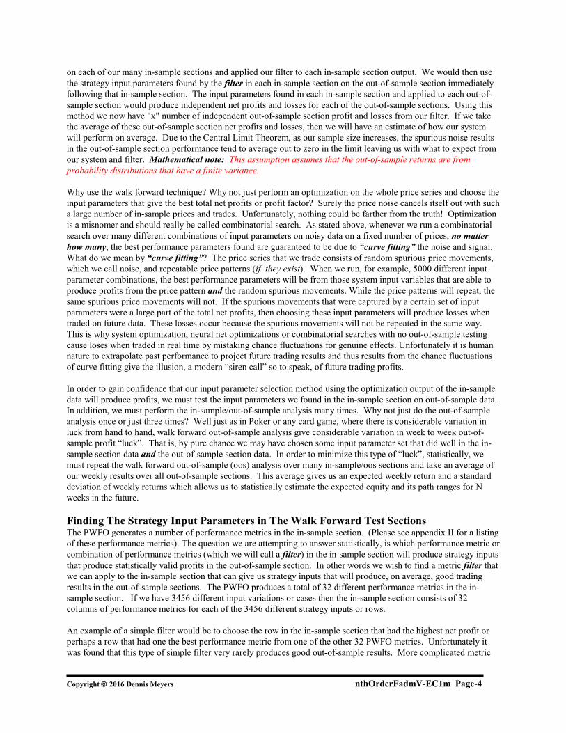
on each of our many in-sample sections and applied our filter to each in-sample section output. We would then use the strategy input parameters found by the filter in each in-sample section on the out-of-sample section immediately following that in-sample section. The input parameters found in each in-sample section and applied to each out-of-sample section would produce independent net profits and losses for each of the out-of-sample sections. Using this method we now have "x" number of independent out-of-sample section profit and losses from our filter. If we take the average of these out-of-sample section net profits and losses, then we will have an estimate of how our system will perform on average. Due to the Central Limit Theorem, as our sample size increases, the spurious noise results in the out-of-sample section performance tend to average out to zero in the limit leaving us with what to expect from our system and filter. Mathematical note: This assumption assumes that the out-of-sample returns are from probability distributions that have a finite variance. Why use the walk forward technique? Why not just perform an optimization on the whole price series and choose the input parameters that give the best total net profits or profit factor? Surely the price noise cancels itself out with such a large number of in-sample prices and trades. Unfortunately, nothing could be farther from the truth! Optimization is a misnomer and should really be called combinatorial search. As stated above, whenever we run a combinatorial search over many different combinations of input parameters on noisy data on a fixed number of prices, no matter how many, the best performance parameters found are guaranteed to be due to “curve fitting” the noise and signal. What do we mean by “curve fitting”? The price series that we trade consists of random spurious price movements, which we call noise, and repeatable price patterns (if they exist). When we run, for example, 5000 different input parameter combinations, the best performance parameters will be from those system input variables that are able to produce profits from the price pattern and the random spurious movements. While the price patterns will repeat, the same spurious price movements will not. If the spurious movements that were captured by a certain set of input parameters were a large part of the total net profits, then choosing these input parameters will produce losses when traded on future data. These losses occur because the spurious movements will not be repeated in the same way. This is why system optimization, neural net optimizations or combinatorial searches with no out-of-sample testing cause loses when traded in real time by mistaking chance fluctuations for genuine effects. Unfortunately it is human nature to extrapolate past performance to project future trading results and thus results from the chance fluctuations of curve fitting give the illusion, a modern “siren call” so to speak, of future trading profits. In order to gain confidence that our input parameter selection method using the optimization output of the in-sample data will produce profits, we must test the input parameters we found in the in-sample section on out-of-sample data. In addition, we must perform the in-sample/out-of-sample analysis many times. Why not just do the out-of-sample analysis once or just three times? Well just as in Poker or any card game, where there is considerable variation in luck from hand to hand, walk forward out-of-sample analysis give considerable variation in week to week out-of-sample profit “luck”. That is, by pure chance we may have chosen some input parameter set that did well in the in-sample section data and the out-of-sample section data. In order to minimize this type of “luck”, statistically, we must repeat the walk forward out-of-sample (oos) analysis over many in-sample/oos sections and take an average of our weekly results over all out-of-sample sections. This average gives us an expected weekly return and a standard deviation of weekly returns which allows us to statistically estimate the expected equity and its path ranges for N weeks in the future. Finding The Strategy Input Parameters in The Walk Forward Test Sections The PWFO generates a number of performance metrics in the in-sample section. (Please see appendix II for a listing of these performance metrics). The question we are attempting to answer statistically, is which performance metric or combination of performance metrics (which we will call a filter) in the in-sample section will produce strategy inputs that produce statistically valid profits in the out-of-sample section. In other words we wish to find a metric filter that we can apply to the in-sample section that can give us strategy inputs that will produce, on average, good trading results in the out-of-sample sections. The PWFO produces a total of 32 different performance metrics in the in-sample section. If we have 3456 different input variations or cases then the in-sample section consists of 32 columns of performance metrics for each of the 3456 different strategy inputs or rows. An example of a simple filter would be to choose the row in the in-sample section that had the highest net profit or perhaps a row that had one the best performance metric from one of the other 32 PWFO metrics. Unfortunately it was found that this type of simple filter very rarely produces good out-of-sample results. More complicated metric


filters can produce good out-of-sample results minimizing spurious price movement biases in the selection of strategy inputs. Here is a combination filter that is used in this paper with good out-of-sample results. High profit factors (PF) in the in-sample section usually mean poor performance in the out-of-sample-section. This is a kind of reversion to the mean. So in the in-sample section we eliminate all strategy input rows that have a PF>3 . The PWFO generates the metric nT. This metric is the sample number of Trades in the In-Sample Section. Let us choose the 50 rows in the in-sample section that contain the lowest(bottom) number of trades from the rows that are left from the PF elimination. This particular filter will now leave 50 cases or rows in the in-sample section that satisfy the above filter conditions. Suppose for this filter, within the 50 in-sample rows that are left, we want the row that has the maximum PWFO metric eq2b1 in the in-sample section. eq2b1 = Slope(b1) of the In-Sample Equity Curve fit by a Least Squares 2nd Order Polynomial Line (b0+ b1*i +b2*i2) to the in-sample equity curve. This would produce a filter named b50nT |p<3-eq2b1. This in-sample filter leaves only one row in the PWFO in-sample section with its associated strategy inputs and out-of-sample net profit in the out-of-sample section. This particular b50nT |p<3-eq2b1 filter finds the strategy inputs parameters in each of the 419 in-sample sections and applies these inputs to each of the 419 out-of-sample sections. Using the filter in-sample strategy inputs on the 419 out-of-sample sections, the average out-of-sample performance is calculated. In addition many other important out-of-sample performance statistics for this filter are calculated and summarized. Figure 3 shows such a filter computer run along with a small sample of other filter combinations that are constructed in a similar manner. Row 10 of the sample output in Figure 3 shows the results of the filter discussed above. A total of 28830 different metric filters were examined. We chose Row 10 because it had a lower BE, BLW and Dev^2 and a higher eqR2 along with better statistics than the rows above it. More on this below and on how that number of filters combinations effect the probability that the filter chosen was or was not due to chance Bootstrap Probability of Filter Results: Using modern "Bootstrap" techniques, we can calculate the probability of obtaining each filter's total out-of-sample net profits by chance. By net we mean subtracting the cost and slippage of all round trip trades from the total out-of-sample profits. Here is how the bootstrap technique is applied. Suppose as an example, we calculate the total out-of-sample net profits(tOnpNet) over all out-of-sample weeks for a given filter like above. A mirror filter is created. However, instead of picking an out-of-sample net profit(OSNP) from a row that the filter picks, the mirror filter picks a random row's OSNP in each of the 419 PWFO files. Suppose we repeat this random row section 5000 times. Each of the 5000 mirror filters will choose a random row's OSNP of their own in each of the 419 PWFO files. At the end, each of the 5000 mirror filters will have 419 random OSNP's picked from the rows of the 419 PWFO files. The sum of the 419 random OSNP picks for each mirror filter will generate a random total out-of-sample net profit(tOnpNet). The average and standard deviation of the 5000 mirror filter's different random tOnpNets will allow us to calculate the chance probability for each our filter's tOnpNet. Thus given the mirror filter's bootstrap random tOnpNet average and standard deviation, we can calculate the probability of obtaining our filter's tOnpNet by pure chance alone. Since for this run we examined 28830(shown in Figure 3) different filters, we can calculate the expected number of cases that we could obtain by pure chance that would match or exceed the tOnpNet of the filter we have chosen or (28830) X (tOnpNet Probability). For our filter in row 10 in Figure 3 the expected number of cases that we could obtain by pure chance that would match or exceed the tOnpNet of $53,236 of Row 10 is 28830 x 7.71 10-7 = 0.022. This is much less than one case so it is improbable that our result was due to pure chance. Results Table 1 on page 8 below presents a table of the 419 in-sample and out-of-sample windows, the selected optimum parameters and the weekly out-of-sample results using the filter described above. Figure 1 presents a graph of the equity and net equity curves generated by using the filter on the 419 weeks ending 1/4/08 to 1/8/16. The equity curves are plotted from the Equity and Net Equity columns in Table 1. Plotted on the equity curves are 2nd Order Polynomial fits. The blue line is the equity curve without commissions and the red dots on the blue line are new highs in equity. The brown line is the net equity curve with commissions and the green dots are the new highs in net equity. The grey line is the weekly EC prices superimposed on the equity chart. Figure 2 Walk Forward Out-Of-Sample Performance for EC Fading Memory Polynomial Velocity System


1 minute bar chart of EC from 12/4/15-12/4/2015 Figure 3 Partial output of the Walk Forward Metric Performance Explorer (WFME) Run on the 419 PWFO files of the EC 1min bars Nth Order Fading Memory Velocity System Discussion of System Performance In Figure 3 Row 10 of the spreadsheet filter output are some statistics that are of interest for our filter. BE is the break even weeks. Assuming the trade average and standard deviation for this filter are from a normal distribution, this is how many weeks we need to trade this strategy so that we have a 98% probability that the equity paths after that number of weeks will be greater than zero. BE is 47.5 weeks for this filter. This means we would have to trade this strategy for at least 47.5 weeks to have a 98% probability that our equity would be positive. Another interesting statistic is Blw. Blw is the maximum number of weeks the OSNP equity curve failed to make a new high. Blw is 28 weeks for this filter. This means that 28 weeks was the longest time that the equity for this strategy failed to make a new equity high. To see the effect of walk forward analysis, take a look at Table 1. Notice how the input parameters pw, N, vup and vdn take sudden jumps from high to low and back. This is the walk forward process quickly adapting to changing volatility conditions in the in-sample sample. In addition, notice how often degree changes from a straight line velocity with degree=1 to a 2nd, 3rd and 4th order velocity with degree= 2, 3 and 4. The 3rd and 4th order velocities, due to the higher order components, change much faster than the straight line velocity. When the data gets very noisy with a lot of spurious price movements, it’s better to have the velocity change slower filtering out the noisy data. During other times when the noise level is not as much it is better to have the velocity break its vup and vdn barriers faster to get onboard a trend faster. This is what the filter is doing. When there is a lot of noise in the in-sample section it switches to the 1st or 2nd order curve velocity. When the noise level is lower in the in-sample section, it switches to the faster changing 3rd or 4th order curve velocity. Using this filter, the strategy was able to generate $53,236 net equity after commissions and slippage trading one EC contract for 419 weeks. Note $20 roundtrip commission and slippage was subtracted from each trade and no positions were carried overnight. The largest losing week was -$2175 and the largest drawdown was -$4013. The longest time between new equity highs was 28 weeks. In observing Table 1 we can see that this strategy and filter made trades from a low of no trades/week to a high of 18 trades/week with an average of 1.8 trades/week on the weeks it did trade. The strategy seemed to wait for really strong trends and then initiate a buy or sell. There were many weeks that had no trades. Out of the 419 out-of-sample weeks the filter only traded 230 of those weeks or 55% of the time with 60% of all trades profitable. In observing the Equity Curve plot in Figure 1 we can see that the equity did quite well in both big up and down moves of the EC. In observing the chart from 12/3/2015 we can see the strategy trading mostly only when there is a big trend action. Given 24 hour trading of the Euro, restricting the strategy to trade only from 7am to 1:50pm caused the strategy to miss many profitable trends opportunities when Asia and then Europe opened trading in the early morning. Further research will include the A.M. time zones. Disclaimer The strategies, methods and indicators presented here are given for educational purposes only and should not be construed as investment advice. Be aware that the profitable performance presented here is based upon hypothetical trading with the benefit of hindsight and can in no way be assumed nor can it be claimed that the strategy and methods presented here will be profitable in the future or that they will not result in losses. References

1. Efron, B., Tibshirani, R.J., (1993), “An Introduction to the Bootstrap”, New York, Chapman & Hall/CRC. 2. Morrison, Norman “Introduction to Sequential Smoothing and Prediction", McGraw-Hill Book Company,

New York, 1969.


Figure 1 Graph of Net Equity Curve Applying the Walk Forward Filter Each Week On EC 1min Bar Prices 01/04/08 – 01/08/16

Note: The blue line is the equity curve without commissions and the red dots on the blue line are new highs in equity. The brown line is the equity curve with commissions and the green dots are the new highs in net equity The grey line is the EC Weekly Closing prices superimposed on the Equity Chart.


Figure 2 Walk Forward Out-Of-Sample Performance for EC Fading Memory Polynomial Velocity System 1 minute bar chart of EC from 12/3/16-12/4/16


Figure 3 Partial output of the Walk Forward Metric Performance Explorer (WFME) EC1 min bars Nth Order Fading Memory Velocity System

The WFME Filter Output Columns are defined as follows:

Row 1 EC1FadmV is the strategy abbreviation, First OOS Week End Date(1/4/08), Last OOS Week End Date(01/08/16), Number of weeks(#419) a=average of bootstrap random picks. s= standard deviation of bootstrap random picks. f=number of different filters examined. c= slippage and round trip trade cost(c=$20).

Filter = The filter that was run. Row10 filter b50nT|p<3-eq2b1 The b50nT|p<3-eq2b1filter produced the following average 419 week statistics on row 10. tOnp = Total out-of-sample(oos) net profit for these 419 weeks. aOsp = Average oos net profit for the 419 weeks aOTrd = Average oos profit per trade aO#T = Average number of oos trades per week B0 = The 419 week trend of the out-of-sample weekly profits %P = The percentage of oos weeks that were traded that were profitable t = The student t statistic for the 419 weekly oos profits. The higher the t statistic the higher the probability that this result was not due to pure chance std = The standard deviation of the 419 weekly oos profits llp = The largest losing oos period(week) eqDD = The oos equity drawdown lr = The largest number of losing oos weeks in a row # = The number of weeks this filter produced a weekly result. Note for some weeks there can be no strategy inputs that satisfy a given filter's criteria. eqTrn = The straight line trend of the oos gross profit equity curve in $/week. eqV^2 = The ending velocity of 2nd order polynomial that is fit to the equity curve eqR2 = The correlation coefficient(r2) of a straight line fit to the equity curve


Dev^2 = A measure of equity curve smoothness. The square root of the average [(equity curve minus a straight line)2] Blw = The maximum number of weeks the oos equity curve failed to make a new high. BE = Break even weeks. Assuming the average and standard deviation are from a normal distribution, this is the number of weeks you would have to trade to have a 98% probability that your oos equity is above zero. tOnpNet = Total out-of-sample net profit(tOnpNet) minus the total trade cost. tOnpNet=tOnp – (Number of trade weeks)*aOnT*Cost. Prob = the probability that the filter's tOnpNet was due to pure chance.


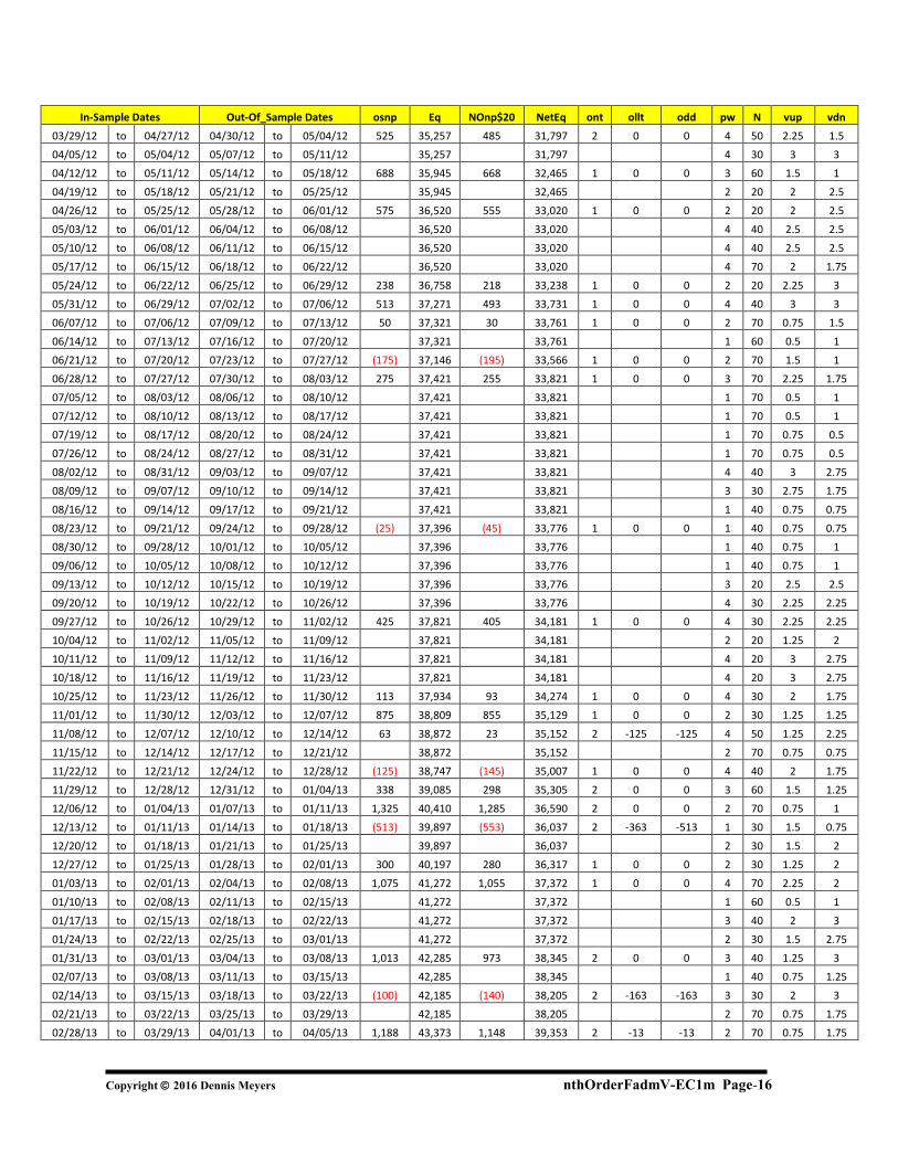
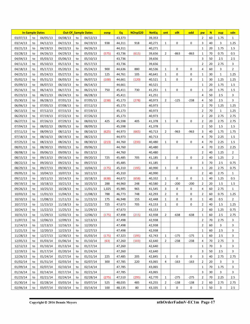
Table 1 Walk Forward Out-Of-Sample Performance Summary for

EC Nth Order Fading Memory Polynomial Velocity System EC-1 min bars 1/2/2008 - 01/08/2016. The input values degree(pw), N, vup, vdn are the values found from applying the filter to the in-sample section optimization runs. Filter= b50nT |p<2.5|lr3-eq2b1 PF<=2.5, LR<=3 and Bottom 50 nT and then maximum eq2b1 osnp = Weekly Out-of-sample gross profit in $ Equity = Running Sum of weekly out-of-sample gross profits $ NOnp$20 = Weekly Out-Of-Sample Net Profit in $ = osnp-ont*20. NetEq = running sum of the weekly out-of-sample net profits in $ ollt = The largest losing trade in the out-of-sample section in $. odd = The drawdown in the out-of-sample section in $. ont = The number of trades in the out-of-sample week. pw= degree, degree=1 for straight line velocity, degree=2 for 2nd order velocity, etc. N = N the lookback period vup, the threshold amount that velocity has to be greater than to issue a buy signal vdn, the threshold amount that velocity has to be less than to issue a sell signal Note: Blank rows indicate that no out-of-sample trades were made that week

In-Sample Dates Out-Of_Sample Dates osnp Eq NOnp$20 NetEq ont ollt odd pw N vup vdn

11/29/07 to 12/28/07 12/31/07 to 01/04/08 238 238 198 198 2 -400 -400 1 70 0.5 0.5

12/06/07 to 01/04/08 01/07/08 to 01/11/08 738 976 718 916 1 0 0 2 60 1 1.5

12/13/07 to 01/11/08 01/14/08 to 01/18/08 563 1,539 543 1,459 1 0 0 1 20 1.25 1.75

12/20/07 to 01/18/08 01/21/08 to 01/25/08 1,539 1,459 1 60 1 0.75

12/27/07 to 01/25/08 01/28/08 to 02/01/08 (13) 1,526 (33) 1,426 1 0 0 1 60 1 0.75

01/03/08 to 02/01/08 02/04/08 to 02/08/08 1,526 1,426 2 70 1.5 1.25

01/10/08 to 02/08/08 02/11/08 to 02/15/08 1,526 1,426 2 70 1.25 1.25

01/17/08 to 02/15/08 02/18/08 to 02/22/08 313 1,839 293 1,719 1 0 0 3 70 1 2

01/24/08 to 02/22/08 02/25/08 to 02/29/08 1,839 1,719 2 70 1 1.25

01/31/08 to 02/29/08 03/03/08 to 03/07/08 613 2,452 573 2,292 2 0 0 1 20 1.5 0.75

02/07/08 to 03/07/08 03/10/08 to 03/14/08 488 2,940 448 2,740 2 0 0 1 60 0.5 0.75

02/14/08 to 03/14/08 03/17/08 to 03/21/08 (138) 2,802 (158) 2,582 1 0 0 2 30 3 2.25

02/21/08 to 03/21/08 03/24/08 to 03/28/08 2,802 2,582 2 30 3 2.5

02/28/08 to 03/28/08 03/31/08 to 04/04/08 2,802 2,582 2 30 3 2.5

03/06/08 to 04/04/08 04/07/08 to 04/11/08 2,802 2,582 2 30 3 2.5

03/13/08 to 04/11/08 04/14/08 to 04/18/08 2,802 2,582 1 30 1 1.25

03/20/08 to 04/18/08 04/21/08 to 04/25/08 2,802 2,582 4 70 2.5 2.25

03/27/08 to 04/25/08 04/28/08 to 05/02/08 (475) 2,327 (495) 2,087 1 0 0 4 70 2.5 2.25

04/03/08 to 05/02/08 05/05/08 to 05/09/08 2,327 2,087 2 30 2 3

04/10/08 to 05/09/08 05/12/08 to 05/16/08 2,327 2,087 4 60 2.25 2.75

04/17/08 to 05/16/08 05/19/08 to 05/23/08 2,327 2,087 4 60 2.25 2.75

04/24/08 to 05/23/08 05/26/08 to 05/30/08 2,327 2,087 2 40 1.5 1.75

05/01/08 to 05/30/08 06/02/08 to 06/06/08 2,413 4,740 2,353 4,440 3 -175 -175 1 70 0.5 0.75

05/08/08 to 06/06/08 06/09/08 to 06/13/08 588 5,328 568 5,008 1 0 0 1 70 1.25 0.5

05/15/08 to 06/13/08 06/16/08 to 06/20/08 5,328 5,008 3 50 2 2.25

05/22/08 to 06/20/08 06/23/08 to 06/27/08 (163) 5,165 (203) 4,805 2 -488 -488 2 50 1 3

05/29/08 to 06/27/08 06/30/08 to 07/04/08 1,438 6,603 1,418 6,223 1 0 0 3 60 1.5 2

06/05/08 to 07/04/08 07/07/08 to 07/11/08 288 6,891 228 6,451 3 -50 -50 2 50 1 2.75

06/12/08 to 07/11/08 07/14/08 to 07/18/08 6,891 6,451 3 30 3 2.75

06/19/08 to 07/18/08 07/21/08 to 07/25/08 6,891 6,451 3 50 2 2.5



06/26/08 to 07/25/08 07/28/08 to 08/01/08 (1,075) 5,816 (1,135) 5,316 3 -1050 -1500 3 30 3 2.75

07/03/08 to 08/01/08 08/04/08 to 08/08/08 5,816 5,316 3 50 2.25 2.5

07/10/08 to 08/08/08 08/11/08 to 08/15/08 5,816 5,316 2 30 2.25 2.25

07/17/08 to 08/15/08 08/18/08 to 08/22/08 5,816 5,316 2 30 2 2.25

07/24/08 to 08/22/08 08/25/08 to 08/29/08 5,816 5,316 2 30 2 2.25

07/31/08 to 08/29/08 09/01/08 to 09/05/08 225 6,041 205 5,521 1 0 0 2 40 2 1.5

08/07/08 to 09/05/08 09/08/08 to 09/12/08 613 6,654 573 6,094 2 0 0 4 50 2.75 2.25

08/14/08 to 09/12/08 09/15/08 to 09/19/08 1,113 7,767 1,013 7,107 5 -1413 -1525 3 30 3 2.5

08/21/08 to 09/19/08 09/22/08 to 09/26/08 (563) 7,204 (603) 6,504 2 -1013 -1013 1 40 1.75 0.75

08/28/08 to 09/26/08 09/29/08 to 10/03/08 (863) 6,341 (963) 5,541 5 -1275 -1275 2 50 2.5 1.25

09/04/08 to 10/03/08 10/06/08 to 10/10/08 (663) 5,678 (763) 4,778 5 -1563 -3488 1 30 1.5 1

09/11/08 to 10/10/08 10/13/08 to 10/17/08 5,678 4,778 3 70 2.75 3

09/18/08 to 10/17/08 10/20/08 to 10/24/08 (1,750) 3,928 (1,770) 3,008 1 0 0 1 20 2 2.75

09/25/08 to 10/24/08 10/27/08 to 10/31/08 688 4,616 648 3,656 2 0 0 2 50 1.5 3

10/02/08 to 10/31/08 11/03/08 to 11/07/08 213 4,829 153 3,809 3 -150 -150 4 70 3 3

10/09/08 to 11/07/08 11/10/08 to 11/14/08 1,050 5,879 1,030 4,839 1 0 0 1 50 2 1

10/16/08 to 11/14/08 11/17/08 to 11/21/08 (2,125) 3,754 (2,145) 2,694 1 0 0 1 30 1.75 2

10/23/08 to 11/21/08 11/24/08 to 11/28/08 400 4,154 380 3,074 1 0 0 1 30 1.75 2

10/30/08 to 11/28/08 12/01/08 to 12/05/08 4,154 3,074 2 70 3 1.75

11/06/08 to 12/05/08 12/08/08 to 12/12/08 4,154 3,074 2 70 3 1.75

11/13/08 to 12/12/08 12/15/08 to 12/19/08 2,675 6,829 2,635 5,709 2 -175 -175 1 30 3 1.25

11/20/08 to 12/19/08 12/22/08 to 12/26/08 6,829 5,709 1 40 2 2.5

11/27/08 to 12/26/08 12/29/08 to 01/02/09 6,829 5,709 2 50 2.25 3

12/04/08 to 01/02/09 01/05/09 to 01/09/09 1,800 8,629 1,780 7,489 1 0 0 1 60 2.5 1

12/11/08 to 01/09/09 01/12/09 to 01/16/09 8,629 7,489 2 70 2 2.75

12/18/08 to 01/16/09 01/19/09 to 01/23/09 8,629 7,489 1 20 2.75 3

12/25/08 to 01/23/09 01/26/09 to 01/30/09 (775) 7,854 (835) 6,654 3 -400 -775 2 50 2.75 2

01/01/09 to 01/30/09 02/02/09 to 02/06/09 7,854 6,654 1 30 2.25 1.75

01/08/09 to 02/06/09 02/09/09 to 02/13/09 7,854 6,654 2 40 3 3

01/15/09 to 02/13/09 02/16/09 to 02/20/09 1,313 9,167 1,293 7,947 1 0 0 2 40 2 2.75

01/22/09 to 02/20/09 02/23/09 to 02/27/09 (363) 8,804 (383) 7,564 1 0 0 2 40 2 2.75

01/29/09 to 02/27/09 03/02/09 to 03/06/09 8,804 7,564 1 30 3 1.25

02/05/09 to 03/06/09 03/09/09 to 03/13/09 (2,138) 6,666 (2,158) 5,406 1 0 0 2 30 2.75 3

02/12/09 to 03/13/09 03/16/09 to 03/20/09 4,175 10,841 4,135 9,541 2 0 0 1 60 0.75 1

02/19/09 to 03/20/09 03/23/09 to 03/27/09 (438) 10,403 (458) 9,083 1 0 0 1 20 2 2

02/26/09 to 03/27/09 03/30/09 to 04/03/09 10,403 9,083 1 20 3 2

03/05/09 to 04/03/09 04/06/09 to 04/10/09 10,403 9,083 1 20 3 2

03/12/09 to 04/10/09 04/13/09 to 04/17/09 10,403 9,083 1 20 3 1.75

03/19/09 to 04/17/09 04/20/09 to 04/24/09 10,403 9,083 1 30 1.5 1.5

03/26/09 to 04/24/09 04/27/09 to 05/01/09 413 10,816 393 9,476 1 0 0 1 30 1.25 1.25

04/02/09 to 05/01/09 05/04/09 to 05/08/09 10,816 9,476 1 60 1 0.75

04/09/09 to 05/08/09 05/11/09 to 05/15/09 10,816 9,476 4 70 3 2.25

04/16/09 to 05/15/09 05/18/09 to 05/22/09 338 11,154 298 9,774 2 0 0 3 70 2 1.75

04/23/09 to 05/22/09 05/25/09 to 05/29/09 11,154 9,774 2 60 2 1.25

04/30/09 to 05/29/09 06/01/09 to 06/05/09 1,913 13,067 1,893 11,667 1 0 0 4 60 3 2.5

05/07/09 to 06/05/09 06/08/09 to 06/12/09 1,463 14,530 1,443 13,110 1 0 0 1 40 1 2

05/14/09 to 06/12/09 06/15/09 to 06/19/09 14,530 13,110 1 20 1.75 3

05/21/09 to 06/19/09 06/22/09 to 06/26/09 14,530 13,110 1 20 1.75 3

05/28/09 to 06/26/09 06/29/09 to 07/03/09 14,530 13,110 1 50 0.75 1.75



06/04/09 to 07/03/09 07/06/09 to 07/10/09 14,530 13,110 1 50 0.75 1.75

06/11/09 to 07/10/09 07/13/09 to 07/17/09 14,530 13,110 4 50 3 2.25

06/18/09 to 07/17/09 07/20/09 to 07/24/09 14,530 13,110 4 50 3 2.25

06/25/09 to 07/24/09 07/27/09 to 07/31/09 213 14,743 193 13,303 1 0 0 4 50 2 2.75

07/02/09 to 07/31/09 08/03/09 to 08/07/09 2,075 16,818 2,035 15,338 2 0 0 4 50 2.5 2

07/09/09 to 08/07/09 08/10/09 to 08/14/09 16,818 15,338 1 50 0.75 1

07/16/09 to 08/14/09 08/17/09 to 08/21/09 900 17,718 880 16,218 1 0 0 1 30 0.75 1.5

07/23/09 to 08/21/09 08/24/09 to 08/28/09 500 18,218 480 16,698 1 0 0 2 30 2.25 2.25

07/30/09 to 08/28/09 08/31/09 to 09/04/09 (663) 17,555 (703) 15,995 2 -1375 -1375 2 50 2.25 1.25

08/06/09 to 09/04/09 09/07/09 to 09/11/09 17,555 15,995 1 70 0.75 0.75

08/13/09 to 09/11/09 09/14/09 to 09/18/09 17,555 15,995 3 70 3 1.5

08/20/09 to 09/18/09 09/21/09 to 09/25/09 713 18,268 693 16,688 1 0 0 3 70 3 1.5

08/27/09 to 09/25/09 09/28/09 to 10/02/09 18,268 16,688 1 30 2 1

09/03/09 to 10/02/09 10/05/09 to 10/09/09 18,268 16,688 3 60 1.75 2

09/10/09 to 10/09/09 10/12/09 to 10/16/09 18,268 16,688 1 60 1 0.5

09/17/09 to 10/16/09 10/19/09 to 10/23/09 18,268 16,688 1 60 1 0.5

09/24/09 to 10/23/09 10/26/09 to 10/30/09 1,500 19,768 1,460 18,148 2 0 0 1 60 1 0.5

10/01/09 to 10/30/09 11/02/09 to 11/06/09 (700) 19,068 (720) 17,428 1 0 0 2 30 2 2

10/08/09 to 11/06/09 11/09/09 to 11/13/09 19,068 17,428 4 60 2 2.5

10/15/09 to 11/13/09 11/16/09 to 11/20/09 (1,138) 17,930 (1,158) 16,270 1 0 0 4 60 2 2.5

10/22/09 to 11/20/09 11/23/09 to 11/27/09 17,930 16,270 4 60 2 3

10/29/09 to 11/27/09 11/30/09 to 12/04/09 2,063 19,993 2,043 18,313 1 0 0 4 60 2 3

11/05/09 to 12/04/09 12/07/09 to 12/11/09 (763) 19,230 (783) 17,530 1 0 0 1 50 0.5 1.5

11/12/09 to 12/11/09 12/14/09 to 12/18/09 19,230 17,530 3 50 1.75 3

11/18/09 to 12/17/09 12/20/09 to 12/24/09 19,230 17,530 3 50 1.75 3

11/25/09 to 12/24/09 12/27/09 to 12/31/09 (413) 18,817 (453) 17,077 2 -338 -413 2 20 1.75 2.75

12/03/09 to 01/01/10 01/04/10 to 01/08/10 975 19,792 955 18,032 1 0 0 3 50 1.75 3

12/10/09 to 01/08/10 01/11/10 to 01/15/10 19,792 18,032 2 50 2.75 1.5

12/17/09 to 01/15/10 01/18/10 to 01/22/10 (1,300) 18,492 (1,360) 16,672 3 -838 -1300 3 40 2 1.75

12/24/09 to 01/22/10 01/25/10 to 01/29/10 18,492 16,672 1 30 2 1

12/31/09 to 01/29/10 02/01/10 to 02/05/10 18,492 16,672 1 50 0.75 0.75

01/07/10 to 02/05/10 02/08/10 to 02/12/10 663 19,155 603 17,275 3 -13 -13 2 40 1 2

01/14/10 to 02/12/10 02/15/10 to 02/19/10 1,500 20,655 1,440 18,715 3 0 0 2 30 1.25 2.25

01/21/10 to 02/19/10 02/22/10 to 02/26/10 20,655 18,715 3 40 2.5 3

01/28/10 to 02/26/10 03/01/10 to 03/05/10 20,655 18,715 3 40 2.5 2.75

02/04/10 to 03/05/10 03/08/10 to 03/12/10 20,655 18,715 3 30 3 3

02/11/10 to 03/12/10 03/15/10 to 03/19/10 (75) 20,580 (95) 18,620 1 0 0 3 60 2 1.25

02/18/10 to 03/19/10 03/22/10 to 03/26/10 20,580 18,620 1 70 0.75 0.5

02/25/10 to 03/26/10 03/29/10 to 04/02/10 20,580 18,620 1 70 0.75 0.5

03/04/10 to 04/02/10 04/05/10 to 04/09/10 (188) 20,392 (208) 18,412 1 0 0 1 70 0.5 0.5

03/11/10 to 04/09/10 04/12/10 to 04/16/10 20,392 18,412 4 50 3 2

03/18/10 to 04/16/10 04/19/10 to 04/23/10 725 21,117 705 19,117 1 0 0 3 70 1 1.75

03/25/10 to 04/23/10 04/26/10 to 04/30/10 225 21,342 165 19,282 3 -513 -513 1 40 1 0.5

04/01/10 to 04/30/10 05/03/10 to 05/07/10 988 22,330 928 20,210 3 -113 -113 3 60 2 1.5

04/08/10 to 05/07/10 05/10/10 to 05/14/10 22,330 20,210 3 70 1.5 2.25

04/15/10 to 05/14/10 05/17/10 to 05/21/10 4,475 26,805 4,395 24,605 4 -75 -75 1 40 0.5 1.5

04/22/10 to 05/21/10 05/24/10 to 05/28/10 26,805 24,605 2 60 2.5 1.5

04/29/10 to 05/28/10 05/31/10 to 06/04/10 1,013 27,818 993 25,598 1 0 0 1 70 1.25 0.5

05/06/10 to 06/04/10 06/07/10 to 06/11/10 27,818 25,598 1 30 1.5 1.75



05/13/10 to 06/11/10 06/14/10 to 06/18/10 27,818 25,598 4 70 2 2.75

05/20/10 to 06/18/10 06/21/10 to 06/25/10 (650) 27,168 (670) 24,928 1 0 0 4 70 2 2.75

05/27/10 to 06/25/10 06/28/10 to 07/02/10 27,168 24,928 2 70 1.25 1.75

06/03/10 to 07/02/10 07/05/10 to 07/09/10 27,168 24,928 2 70 1 1

06/10/10 to 07/09/10 07/12/10 to 07/16/10 27,168 24,928 3 40 2.5 1.75

06/17/10 to 07/16/10 07/19/10 to 07/23/10 (1,088) 26,080 (1,128) 23,800 2 -1288 -1288 4 40 3 2

06/24/10 to 07/23/10 07/26/10 to 07/30/10 26,080 23,800 4 60 2.5 2.25

07/01/10 to 07/30/10 08/02/10 to 08/06/10 513 26,593 493 24,293 1 0 0 2 50 1.25 1.5

07/08/10 to 08/06/10 08/09/10 to 08/13/10 450 27,043 430 24,723 1 0 0 2 20 3 3

07/15/10 to 08/13/10 08/16/10 to 08/20/10 (138) 26,905 (158) 24,565 1 0 0 2 40 3 1.5

07/22/10 to 08/20/10 08/23/10 to 08/27/10 26,905 24,565 2 70 1.5 1.5

07/29/10 to 08/27/10 08/30/10 to 09/03/10 26,905 24,565 2 20 3 2.75

08/05/10 to 09/03/10 09/06/10 to 09/10/10 26,905 24,565 2 20 3 2.75

08/12/10 to 09/10/10 09/13/10 to 09/17/10 825 27,730 805 25,370 1 0 0 2 20 3 2.25

08/19/10 to 09/17/10 09/20/10 to 09/24/10 (125) 27,605 (145) 25,225 1 0 0 1 60 1 0.5

08/26/10 to 09/24/10 09/27/10 to 10/01/10 27,605 25,225 1 70 0.75 0.5

09/02/10 to 10/01/10 10/04/10 to 10/08/10 (450) 27,155 (490) 24,735 2 -588 -588 1 60 0.5 0.5

09/09/10 to 10/08/10 10/11/10 to 10/15/10 27,155 24,735 1 20 1.75 2

09/16/10 to 10/15/10 10/18/10 to 10/22/10 563 27,718 543 25,278 1 0 0 2 50 1.5 1.5

09/23/10 to 10/22/10 10/25/10 to 10/29/10 27,718 25,278 4 60 2.75 3

09/30/10 to 10/29/10 11/01/10 to 11/05/10 27,718 25,278 3 70 2 1.5

10/07/10 to 11/05/10 11/08/10 to 11/12/10 (600) 27,118 (620) 24,658 1 0 0 3 70 2 1.5

10/14/10 to 11/12/10 11/15/10 to 11/19/10 27,118 24,658 3 60 2 1.75

10/21/10 to 11/19/10 11/22/10 to 11/26/10 27,118 24,658 3 70 1.25 2.25

10/28/10 to 11/26/10 11/29/10 to 12/03/10 950 28,068 890 25,548 3 -338 -338 3 70 1.25 2.25

11/04/10 to 12/03/10 12/06/10 to 12/10/10 28,068 25,548 3 60 2.25 2.75

11/11/10 to 12/10/10 12/13/10 to 12/17/10 (313) 27,755 (333) 25,215 1 0 0 1 40 1.25 0.75

11/18/10 to 12/17/10 12/20/10 to 12/24/10 27,755 25,215 3 60 2.25 2.5

11/25/10 to 12/24/10 12/27/10 to 12/31/10 27,755 25,215 3 60 2.25 2.5

12/02/10 to 12/31/10 01/03/11 to 01/07/11 27,755 25,215 4 60 2.5 2.75

12/09/10 to 01/07/11 01/10/11 to 01/14/11 1,325 29,080 1,305 26,520 1 0 0 1 60 0.5 1

12/16/10 to 01/14/11 01/17/11 to 01/21/11 29,080 26,520 2 70 1.5 1

12/23/10 to 01/21/11 01/24/11 to 01/28/11 (588) 28,492 (608) 25,912 1 0 0 1 20 1.75 1.25

12/30/10 to 01/28/11 01/31/11 to 02/04/11 625 29,117 605 26,517 1 0 0 2 30 2 2

01/06/11 to 02/04/11 02/07/11 to 02/11/11 29,117 26,517 1 60 0.5 1

01/13/11 to 02/11/11 02/14/11 to 02/18/11 1,125 30,242 1,085 27,602 2 0 0 2 70 0.75 1.5

01/20/11 to 02/18/11 02/21/11 to 02/25/11 30,242 27,602 3 30 3 2.75

01/27/11 to 02/25/11 02/28/11 to 03/04/11 150 30,392 130 27,732 1 0 0 3 70 1 2.25

02/03/11 to 03/04/11 03/07/11 to 03/11/11 30,392 27,732 2 70 1.75 0.75

02/10/11 to 03/11/11 03/14/11 to 03/18/11 663 31,055 623 28,355 2 0 0 3 70 1 1.25

02/17/11 to 03/18/11 03/21/11 to 03/25/11 (750) 30,305 (810) 27,545 3 -1050 -1050 2 40 1 1.25

02/24/11 to 03/25/11 03/28/11 to 04/01/11 30,305 27,545 2 20 2.5 2.75

03/03/11 to 04/01/11 04/04/11 to 04/08/11 30,305 27,545 2 20 2.5 2.75

03/10/11 to 04/08/11 04/11/11 to 04/15/11 (525) 29,780 (545) 27,000 1 0 0 1 30 1 0.75

03/17/11 to 04/15/11 04/18/11 to 04/22/11 275 30,055 255 27,255 1 0 0 3 60 1.75 1.5

03/24/11 to 04/22/11 04/25/11 to 04/29/11 30,055 27,255 4 60 1.75 2.75

03/31/11 to 04/29/11 05/02/11 to 05/06/11 (1,125) 28,930 (1,185) 26,070 3 -2938 -2938 3 50 1.5 2.75

04/07/11 to 05/06/11 05/09/11 to 05/13/11 28,930 26,070 2 40 1.75 2.25

04/14/11 to 05/13/11 05/16/11 to 05/20/11 28,930 26,070 2 40 1.75 2.25



04/21/11 to 05/20/11 05/23/11 to 05/27/11 28,930 26,070 2 40 1.75 2.25

04/28/11 to 05/27/11 05/30/11 to 06/03/11 28,930 26,070 2 40 1.75 2.25

05/05/11 to 06/03/11 06/06/11 to 06/10/11 250 29,180 230 26,300 1 0 0 2 40 1.75 2.25

05/12/11 to 06/10/11 06/13/11 to 06/17/11 (125) 29,055 (145) 26,155 1 0 0 2 50 1.25 2

05/19/11 to 06/17/11 06/20/11 to 06/24/11 (88) 28,967 (108) 26,047 1 0 0 1 70 0.5 0.75

05/26/11 to 06/24/11 06/27/11 to 07/01/11 (113) 28,854 (153) 25,894 2 -150 -150 1 70 0.5 0.75

06/02/11 to 07/01/11 07/04/11 to 07/08/11 13 28,867 (27) 25,867 2 -163 -163 1 50 1 0.5

06/09/11 to 07/08/11 07/11/11 to 07/15/11 28,867 25,867 3 60 2.25 2.25

06/16/11 to 07/15/11 07/18/11 to 07/22/11 1,500 30,367 1,480 27,347 1 0 0 2 60 1.5 1.25

06/23/11 to 07/22/11 07/25/11 to 07/29/11 30,367 27,347 2 60 2.25 1.25

06/30/11 to 07/29/11 08/01/11 to 08/05/11 763 31,130 723 28,070 2 -163 -163 1 70 1.25 0.5

07/07/11 to 08/05/11 08/08/11 to 08/12/11 31,130 28,070 1 50 1 1.25

07/14/11 to 08/12/11 08/15/11 to 08/19/11 31,130 28,070 1 50 1 1.25

07/21/11 to 08/19/11 08/22/11 to 08/26/11 31,130 28,070 1 50 1 1.25

07/28/11 to 08/26/11 08/29/11 to 09/02/11 31,130 28,070 3 70 2.5 1.75

08/04/11 to 09/02/11 09/05/11 to 09/09/11 1,475 32,605 1,435 29,505 2 0 0 2 40 2.5 1.75

08/11/11 to 09/09/11 09/12/11 to 09/16/11 (63) 32,542 (83) 29,422 1 0 0 4 70 2.5 2.75

08/18/11 to 09/16/11 09/19/11 to 09/23/11 (50) 32,492 (70) 29,352 1 0 0 3 70 2.5 2

08/25/11 to 09/23/11 09/26/11 to 09/30/11 32,492 29,352 1 50 1.25 1

09/01/11 to 09/30/11 10/03/11 to 10/07/11 313 32,805 293 29,645 1 0 0 1 50 1.25 1

09/08/11 to 10/07/11 10/10/11 to 10/14/11 32,805 29,645 1 20 2 2.5

09/15/11 to 10/14/11 10/17/11 to 10/21/11 32,805 29,645 1 20 2 2.5

09/22/11 to 10/21/11 10/24/11 to 10/28/11 938 33,743 918 30,563 1 0 0 2 70 1.25 1.75

09/29/11 to 10/28/11 10/31/11 to 11/04/11 (1,763) 31,980 (1,783) 28,780 1 0 0 1 30 1.75 1.25

10/06/11 to 11/04/11 11/07/11 to 11/11/11 31,980 28,780 2 50 2.25 1.75

10/13/11 to 11/11/11 11/14/11 to 11/18/11 31,980 28,780 1 20 1.75 1.75

10/20/11 to 11/18/11 11/21/11 to 11/25/11 31,980 28,780 1 20 1.75 1.75

10/27/11 to 11/25/11 11/28/11 to 12/02/11 (400) 31,580 (420) 28,360 1 0 0 2 70 1.25 1.5

11/03/11 to 12/02/11 12/05/11 to 12/09/11 63 31,643 43 28,403 1 0 0 4 70 2.5 2.5

11/10/11 to 12/09/11 12/12/11 to 12/16/11 31,643 28,403 1 60 0.5 1

11/17/11 to 12/16/11 12/19/11 to 12/23/11 31,643 28,403 2 40 1.5 2.75

11/24/11 to 12/23/11 12/26/11 to 12/30/11 31,643 28,403 1 20 1 2.25

12/01/11 to 12/30/11 01/02/12 to 01/06/12 31,643 28,403 2 70 0.75 1.75

12/08/11 to 01/06/12 01/09/12 to 01/13/12 388 32,031 368 28,771 1 0 0 2 70 0.75 1.75

12/15/11 to 01/13/12 01/16/12 to 01/20/12 (75) 31,956 (95) 28,676 1 0 0 4 70 1.25 2.75

12/22/11 to 01/20/12 01/23/12 to 01/27/12 1,163 33,119 1,123 29,799 2 0 0 3 70 1 2.25

12/29/11 to 01/27/12 01/30/12 to 02/03/12 (463) 32,656 (483) 29,316 1 0 0 3 40 2.75 1.75

01/05/12 to 02/03/12 02/06/12 to 02/10/12 32,656 29,316 2 30 2.25 2

01/12/12 to 02/10/12 02/13/12 to 02/17/12 32,656 29,316 2 30 2.25 2

01/19/12 to 02/17/12 02/20/12 to 02/24/12 32,656 29,316 2 20 2.75 3

01/26/12 to 02/24/12 02/27/12 to 03/02/12 888 33,544 868 30,184 1 0 0 2 30 2.25 1.5

02/02/12 to 03/02/12 03/05/12 to 03/09/12 33,544 30,184 2 20 2.75 2.5

02/09/12 to 03/09/12 03/12/12 to 03/16/12 488 34,032 468 30,652 1 0 0 2 60 1 1.5

02/16/12 to 03/16/12 03/19/12 to 03/23/12 400 34,432 380 31,032 1 0 0 2 50 1 1.5

02/23/12 to 03/23/12 03/26/12 to 03/30/12 34,432 31,032 1 50 0.75 0.5

03/01/12 to 03/30/12 04/02/12 to 04/06/12 300 34,732 280 31,312 1 0 0 2 50 1.25 1

03/08/12 to 04/06/12 04/09/12 to 04/13/12 34,732 31,312 4 40 2.5 2.5

03/15/12 to 04/13/12 04/16/12 to 04/20/12 34,732 31,312 2 70 1 1.5

03/22/12 to 04/20/12 04/23/12 to 04/27/12 34,732 31,312 4 50 2.25 1.5



03/29/12 to 04/27/12 04/30/12 to 05/04/12 525 35,257 485 31,797 2 0 0 4 50 2.25 1.5

04/05/12 to 05/04/12 05/07/12 to 05/11/12 35,257 31,797 4 30 3 3

04/12/12 to 05/11/12 05/14/12 to 05/18/12 688 35,945 668 32,465 1 0 0 3 60 1.5 1

04/19/12 to 05/18/12 05/21/12 to 05/25/12 35,945 32,465 2 20 2 2.5

04/26/12 to 05/25/12 05/28/12 to 06/01/12 575 36,520 555 33,020 1 0 0 2 20 2 2.5

05/03/12 to 06/01/12 06/04/12 to 06/08/12 36,520 33,020 4 40 2.5 2.5

05/10/12 to 06/08/12 06/11/12 to 06/15/12 36,520 33,020 4 40 2.5 2.5

05/17/12 to 06/15/12 06/18/12 to 06/22/12 36,520 33,020 4 70 2 1.75

05/24/12 to 06/22/12 06/25/12 to 06/29/12 238 36,758 218 33,238 1 0 0 2 20 2.25 3

05/31/12 to 06/29/12 07/02/12 to 07/06/12 513 37,271 493 33,731 1 0 0 4 40 3 3

06/07/12 to 07/06/12 07/09/12 to 07/13/12 50 37,321 30 33,761 1 0 0 2 70 0.75 1.5

06/14/12 to 07/13/12 07/16/12 to 07/20/12 37,321 33,761 1 60 0.5 1

06/21/12 to 07/20/12 07/23/12 to 07/27/12 (175) 37,146 (195) 33,566 1 0 0 2 70 1.5 1

06/28/12 to 07/27/12 07/30/12 to 08/03/12 275 37,421 255 33,821 1 0 0 3 70 2.25 1.75

07/05/12 to 08/03/12 08/06/12 to 08/10/12 37,421 33,821 1 70 0.5 1

07/12/12 to 08/10/12 08/13/12 to 08/17/12 37,421 33,821 1 70 0.5 1

07/19/12 to 08/17/12 08/20/12 to 08/24/12 37,421 33,821 1 70 0.75 0.5

07/26/12 to 08/24/12 08/27/12 to 08/31/12 37,421 33,821 1 70 0.75 0.5

08/02/12 to 08/31/12 09/03/12 to 09/07/12 37,421 33,821 4 40 3 2.75

08/09/12 to 09/07/12 09/10/12 to 09/14/12 37,421 33,821 3 30 2.75 1.75

08/16/12 to 09/14/12 09/17/12 to 09/21/12 37,421 33,821 1 40 0.75 0.75

08/23/12 to 09/21/12 09/24/12 to 09/28/12 (25) 37,396 (45) 33,776 1 0 0 1 40 0.75 0.75

08/30/12 to 09/28/12 10/01/12 to 10/05/12 37,396 33,776 1 40 0.75 1

09/06/12 to 10/05/12 10/08/12 to 10/12/12 37,396 33,776 1 40 0.75 1

09/13/12 to 10/12/12 10/15/12 to 10/19/12 37,396 33,776 3 20 2.5 2.5

09/20/12 to 10/19/12 10/22/12 to 10/26/12 37,396 33,776 4 30 2.25 2.25

09/27/12 to 10/26/12 10/29/12 to 11/02/12 425 37,821 405 34,181 1 0 0 4 30 2.25 2.25

10/04/12 to 11/02/12 11/05/12 to 11/09/12 37,821 34,181 2 20 1.25 2

10/11/12 to 11/09/12 11/12/12 to 11/16/12 37,821 34,181 4 20 3 2.75

10/18/12 to 11/16/12 11/19/12 to 11/23/12 37,821 34,181 4 20 3 2.75

10/25/12 to 11/23/12 11/26/12 to 11/30/12 113 37,934 93 34,274 1 0 0 4 30 2 1.75

11/01/12 to 11/30/12 12/03/12 to 12/07/12 875 38,809 855 35,129 1 0 0 2 30 1.25 1.25

11/08/12 to 12/07/12 12/10/12 to 12/14/12 63 38,872 23 35,152 2 -125 -125 4 50 1.25 2.25

11/15/12 to 12/14/12 12/17/12 to 12/21/12 38,872 35,152 2 70 0.75 0.75

11/22/12 to 12/21/12 12/24/12 to 12/28/12 (125) 38,747 (145) 35,007 1 0 0 4 40 2 1.75

11/29/12 to 12/28/12 12/31/12 to 01/04/13 338 39,085 298 35,305 2 0 0 3 60 1.5 1.25

12/06/12 to 01/04/13 01/07/13 to 01/11/13 1,325 40,410 1,285 36,590 2 0 0 2 70 0.75 1

12/13/12 to 01/11/13 01/14/13 to 01/18/13 (513) 39,897 (553) 36,037 2 -363 -513 1 30 1.5 0.75

12/20/12 to 01/18/13 01/21/13 to 01/25/13 39,897 36,037 2 30 1.5 2

12/27/12 to 01/25/13 01/28/13 to 02/01/13 300 40,197 280 36,317 1 0 0 2 30 1.25 2

01/03/13 to 02/01/13 02/04/13 to 02/08/13 1,075 41,272 1,055 37,372 1 0 0 4 70 2.25 2

01/10/13 to 02/08/13 02/11/13 to 02/15/13 41,272 37,372 1 60 0.5 1

01/17/13 to 02/15/13 02/18/13 to 02/22/13 41,272 37,372 3 40 2 3

01/24/13 to 02/22/13 02/25/13 to 03/01/13 41,272 37,372 2 30 1.5 2.75

01/31/13 to 03/01/13 03/04/13 to 03/08/13 1,013 42,285 973 38,345 2 0 0 3 40 1.25 3

02/07/13 to 03/08/13 03/11/13 to 03/15/13 42,285 38,345 1 40 0.75 1.25

02/14/13 to 03/15/13 03/18/13 to 03/22/13 (100) 42,185 (140) 38,205 2 -163 -163 3 30 2 3

02/21/13 to 03/22/13 03/25/13 to 03/29/13 42,185 38,205 2 70 0.75 1.75

02/28/13 to 03/29/13 04/01/13 to 04/05/13 1,188 43,373 1,148 39,353 2 -13 -13 2 70 0.75 1.75



03/07/13 to 04/05/13 04/08/13 to 04/12/13 43,373 39,353 2 60 1.75 1

03/14/13 to 04/12/13 04/15/13 to 04/19/13 938 44,311 918 40,271 1 0 0 3 40 3 1.25

03/21/13 to 04/19/13 04/22/13 to 04/26/13 44,311 40,271 1 20 1.75 1.5

03/28/13 to 04/26/13 04/29/13 to 05/03/13 (575) 43,736 (615) 39,656 2 -863 -863 1 70 0.75 0.5

04/04/13 to 05/03/13 05/06/13 to 05/10/13 43,736 39,656 3 50 2.5 2.5

04/11/13 to 05/10/13 05/13/13 to 05/17/13 43,736 39,656 2 20 2.75 3

04/18/13 to 05/17/13 05/20/13 to 05/24/13 900 44,636 880 40,536 1 0 0 4 60 3 2

04/25/13 to 05/24/13 05/27/13 to 05/31/13 125 44,761 105 40,641 1 0 0 1 30 1 1.25

05/02/13 to 05/31/13 06/03/13 to 06/07/13 (100) 44,661 (120) 40,521 1 0 0 1 30 1.25 1.25

05/09/13 to 06/07/13 06/10/13 to 06/14/13 44,661 40,521 1 20 1.75 1.5

05/16/13 to 06/14/13 06/17/13 to 06/21/13 750 45,411 730 41,251 1 0 0 1 20 1.75 1.5

05/23/13 to 06/21/13 06/24/13 to 06/28/13 45,411 41,251 4 50 2.5 3

05/30/13 to 06/28/13 07/01/13 to 07/05/13 (238) 45,173 (278) 40,973 2 -125 -238 4 50 2.5 3

06/06/13 to 07/05/13 07/08/13 to 07/12/13 45,173 40,973 2 70 1.25 1.25

06/13/13 to 07/12/13 07/15/13 to 07/19/13 45,173 40,973 2 70 1 1.25

06/20/13 to 07/19/13 07/22/13 to 07/26/13 45,173 40,973 2 20 2.75 2.75

06/27/13 to 07/26/13 07/29/13 to 08/02/13 425 45,598 405 41,378 1 0 0 2 20 2.75 2.75

07/04/13 to 08/02/13 08/05/13 to 08/09/13 45,598 41,378 2 50 1.5 1.5

07/11/13 to 08/09/13 08/12/13 to 08/16/13 (625) 44,973 (665) 40,713 2 -963 -963 3 40 1.75 1.75

07/18/13 to 08/16/13 08/19/13 to 08/23/13 44,973 40,713 4 70 2.25 1.5

07/25/13 to 08/23/13 08/26/13 to 08/30/13 (213) 44,760 (233) 40,480 1 0 0 4 70 2.25 1.5

08/01/13 to 08/30/13 09/02/13 to 09/06/13 44,760 40,480 4 70 2.25 2.25

08/08/13 to 09/06/13 09/09/13 to 09/13/13 44,760 40,480 2 40 1.25 2

08/15/13 to 09/13/13 09/16/13 to 09/20/13 725 45,485 705 41,185 1 0 0 2 40 1.25 2

08/22/13 to 09/20/13 09/23/13 to 09/27/13 45,485 41,185 3 70 2.5 0.75

08/29/13 to 09/27/13 09/30/13 to 10/04/13 (175) 45,310 (195) 40,990 1 0 0 1 20 2.75 0.75

09/05/13 to 10/04/13 10/07/13 to 10/11/13 45,310 40,990 2 40 2.75 1

09/12/13 to 10/11/13 10/14/13 to 10/18/13 (638) 44,672 (658) 40,332 1 0 0 1 40 1.25 0.5

09/19/13 to 10/18/13 10/21/13 to 10/25/13 288 44,960 248 40,580 2 -200 -200 2 20 1.5 1.5

09/26/13 to 10/25/13 10/28/13 to 11/01/13 1,025 45,985 965 41,545 3 0 0 4 60 2.75 1

10/03/13 to 11/01/13 11/04/13 to 11/08/13 788 46,773 748 42,293 2 0 0 2 60 0.75 1.25

10/10/13 to 11/08/13 11/11/13 to 11/15/13 175 46,948 155 42,448 1 0 0 1 40 0.5 2

10/17/13 to 11/15/13 11/18/13 to 11/22/13 725 47,673 705 43,153 1 0 0 2 40 1.5 1.25

10/24/13 to 11/22/13 11/25/13 to 11/29/13 47,673 43,153 2 60 1.25 0.75

10/31/13 to 11/29/13 12/02/13 to 12/06/13 (175) 47,498 (215) 42,938 2 -638 -638 1 60 2.5 2.75

11/07/13 to 12/06/13 12/09/13 to 12/13/13 47,498 42,938 2 70 2.75 3

11/14/13 to 12/13/13 12/16/13 to 12/20/13 47,498 42,938 2 60 3 3

11/21/13 to 12/20/13 12/23/13 to 12/27/13 47,498 42,938 1 60 2.5 3

11/28/13 to 12/27/13 12/30/13 to 01/03/14 (175) 47,323 (195) 42,743 1 -175 -175 1 60 2.5 3

12/05/13 to 01/03/14 01/06/14 to 01/10/14 (63) 47,260 (103) 42,640 2 -238 -238 4 70 2.75 3

12/12/13 to 01/10/14 01/13/14 to 01/17/14 47,260 42,640 1 70 3 3

12/19/13 to 01/17/14 01/20/14 to 01/24/14 47,260 42,640 3 50 2.5 3

12/26/13 to 01/24/14 01/27/14 to 01/31/14 225 47,485 205 42,845 1 0 0 3 40 2.75 2.75

01/02/14 to 01/31/14 02/03/14 to 02/07/14 300 47,785 220 43,065 4 -163 -163 2 20 3 3

01/09/14 to 02/07/14 02/10/14 to 02/14/14 47,785 43,065 1 70 1.75 3

01/16/14 to 02/14/14 02/17/14 to 02/21/14 47,785 43,065 3 30 3 3

01/23/14 to 02/21/14 02/24/14 to 02/28/14 (275) 47,510 (295) 42,770 1 -275 -275 2 70 2.25 2.5

01/30/14 to 02/28/14 03/03/14 to 03/07/14 525 48,035 485 43,255 2 -138 -138 2 60 2.75 2.75

02/06/14 to 03/07/14 03/10/14 to 03/14/14 100 48,135 80 43,335 1 0 0 1 50 3 2.5



02/13/14 to 03/14/14 03/17/14 to 03/21/14 213 48,348 193 43,528 1 0 0 1 40 2.75 3

02/20/14 to 03/21/14 03/24/14 to 03/28/14 (250) 48,098 (290) 43,238 2 -175 -250 1 50 2.75 2.75

02/27/14 to 03/28/14 03/31/14 to 04/04/14 100 48,198 80 43,318 1 0 0 1 70 2.75 2.5

03/06/14 to 04/04/14 04/07/14 to 04/11/14 48,198 43,318 1 70 2.75 2.75

03/13/14 to 04/11/14 04/14/14 to 04/18/14 48,198 43,318 1 60 2.75 1.75

03/20/14 to 04/18/14 04/21/14 to 04/25/14 48,198 43,318 1 70 1.75 3

03/27/14 to 04/25/14 04/28/14 to 05/02/14 (250) 47,948 (310) 43,008 3 -563 -563 4 50 3 2.5

04/03/14 to 05/02/14 05/05/14 to 05/09/14 388 48,336 368 43,376 1 0 0 1 70 2.25 2.25

04/10/14 to 05/09/14 05/12/14 to 05/16/14 48,336 43,376 1 50 2.75 2

04/17/14 to 05/16/14 05/19/14 to 05/23/14 48,336 43,376 1 70 2.5 2.75

04/24/14 to 05/23/14 05/26/14 to 05/30/14 48,336 43,376 1 70 2.5 2.75

05/01/14 to 05/30/14 06/02/14 to 06/06/14 (1,063) 47,273 (1,103) 42,273 2 -1300 -1300 1 70 2.5 2.5

05/08/14 to 06/06/14 06/09/14 to 06/13/14 47,273 42,273 1 40 3 2.5

05/15/14 to 06/13/14 06/16/14 to 06/20/14 47,273 42,273 1 30 2.75 2.5

05/22/14 to 06/20/14 06/23/14 to 06/27/14 (150) 47,123 (170) 42,103 1 -150 -150 1 50 2.25 2.25

05/29/14 to 06/27/14 06/30/14 to 07/04/14 100 47,223 80 42,183 1 0 0 1 30 2.75 2.5

06/05/14 to 07/04/14 07/07/14 to 07/11/14 47,223 42,183 2 70 3 2.75

06/12/14 to 07/11/14 07/14/14 to 07/18/14 (488) 46,735 (528) 41,655 2 -400 -488 2 60 2.75 2

06/19/14 to 07/18/14 07/21/14 to 07/25/14 46,735 41,655 4 40 3 2.25

06/26/14 to 07/25/14 07/28/14 to 08/01/14 (138) 46,597 (178) 41,477 2 -263 -263 2 20 2.5 3

07/03/14 to 08/01/14 08/04/14 to 08/08/14 46,597 41,477 1 20 3 2.5

07/10/14 to 08/08/14 08/11/14 to 08/15/14 (388) 46,209 (408) 41,069 1 -388 -388 2 50 2.25 2.25

07/17/14 to 08/15/14 08/18/14 to 08/22/14 46,209 41,069 2 30 2.5 3

07/24/14 to 08/22/14 08/25/14 to 08/29/14 46,209 41,069 2 30 2.5 3

07/31/14 to 08/29/14 09/01/14 to 09/05/14 1,350 47,559 1,330 42,399 1 0 0 2 30 2.5 3

08/07/14 to 09/05/14 09/08/14 to 09/12/14 (150) 47,409 (170) 42,229 1 -150 -150 1 30 3 2.5

08/14/14 to 09/12/14 09/15/14 to 09/19/14 (250) 47,159 (290) 41,939 2 -175 -250 1 70 1.5 2.5

08/21/14 to 09/19/14 09/22/14 to 09/26/14 113 47,272 93 42,032 1 0 0 1 70 2 2.25

08/28/14 to 09/26/14 09/29/14 to 10/03/14 463 47,735 423 42,455 2 -25 -25 1 50 2.25 2.5

09/04/14 to 10/03/14 10/06/14 to 10/10/14 1,063 48,798 1,023 43,478 2 0 0 3 70 3 2.25

09/11/14 to 10/10/14 10/13/14 to 10/17/14 738 49,536 718 44,196 1 0 0 1 40 2.5 3

09/18/14 to 10/17/14 10/20/14 to 10/24/14 163 49,699 143 44,339 1 0 0 2 60 2.5 2.5

09/25/14 to 10/24/14 10/27/14 to 10/31/14 413 50,112 353 44,692 3 -125 -125 2 60 2.5 2.5

10/02/14 to 10/31/14 11/03/14 to 11/07/14 338 50,450 298 44,990 2 -63 -63 1 30 3 2.75

10/09/14 to 11/07/14 11/10/14 to 11/14/14 588 51,038 528 45,518 3 -513 -513 3 40 3 2.5

10/16/14 to 11/14/14 11/17/14 to 11/21/14 (313) 50,725 (353) 45,165 2 -275 -313 4 50 3 3

10/23/14 to 11/21/14 11/24/14 to 11/28/14 88 50,813 68 45,233 1 0 0 1 70 3 1.25

10/30/14 to 11/28/14 12/01/14 to 12/05/14 463 51,276 403 45,636 3 0 0 1 30 3 2.25

11/06/14 to 12/05/14 12/08/14 to 12/12/14 51,276 45,636 1 70 3 3

11/13/14 to 12/12/14 12/15/14 to 12/19/14 (1,513) 49,763 (1,593) 44,043 4 -950 -1675 1 30 2.5 3

11/20/14 to 12/19/14 12/22/14 to 12/26/14 49,763 44,043 2 70 2.25 3

11/27/14 to 12/26/14 12/29/14 to 01/02/15 49,763 44,043 2 70 2.25 3

12/04/14 to 01/02/15 01/05/15 to 01/09/15 175 49,938 155 44,198 1 0 0 2 70 2.25 3

12/11/14 to 01/09/15 01/12/15 to 01/16/15 (275) 49,663 (335) 43,863 3 -600 -600 1 50 3 2.25

12/18/14 to 01/16/15 01/19/15 to 01/23/15 1,963 51,626 1,903 45,766 3 -163 -163 2 70 2.75 3

12/25/14 to 01/23/15 01/26/15 to 01/30/15 (200) 51,426 (280) 45,486 4 -113 -238 1 70 3 2

01/01/15 to 01/30/15 02/02/15 to 02/06/15 1,563 52,989 1,503 46,989 3 -150 -150 1 70 2.75 2.25

01/08/15 to 02/06/15 02/09/15 to 02/13/15 (825) 52,164 (845) 46,144 1 -825 -825 1 70 2.75 2.25

01/15/15 to 02/13/15 02/16/15 to 02/20/15 563 52,727 523 46,667 2 -150 -150 1 40 2.75 2.5



01/22/15 to 02/20/15 02/23/15 to 02/27/15 1,338 54,065 1,298 47,965 2 -200 -200 1 60 2.75 2.25

01/29/15 to 02/27/15 03/02/15 to 03/06/15 500 54,565 440 48,405 3 0 0 3 70 3 2.25

02/05/15 to 03/06/15 03/09/15 to 03/13/15 (2,175) 52,390 (2,275) 46,130 5 -1088 -2875 1 40 2 3

02/12/15 to 03/13/15 03/16/15 to 03/20/15 1,613 54,003 1,513 47,643 5 -138 -138 2 50 2.5 3

02/19/15 to 03/20/15 03/23/15 to 03/27/15 1,350 55,353 1,270 48,913 4 0 0 1 60 2 2.25

02/26/15 to 03/27/15 03/30/15 to 04/03/15 (113) 55,240 (173) 48,740 3 -388 -388 1 50 2.75 2

03/05/15 to 04/03/15 04/06/15 to 04/10/15 563 55,803 523 49,263 2 -163 -163 1 40 3 2.5

03/12/15 to 04/10/15 04/13/15 to 04/17/15 588 56,391 468 49,731 6 -575 -1025 3 60 3 3

03/19/15 to 04/17/15 04/20/15 to 04/24/15 (388) 56,003 (428) 49,303 2 -325 -388 1 70 3 1.75

03/26/15 to 04/24/15 04/27/15 to 05/01/15 (1,438) 54,565 (1,498) 47,805 3 -1238 -1475 1 70 3 3

04/02/15 to 05/01/15 05/04/15 to 05/08/15 363 54,928 323 48,128 2 0 0 1 70 3 3

04/09/15 to 05/08/15 05/11/15 to 05/15/15 1,125 56,053 1,085 49,213 2 0 0 1 70 3 3

04/16/15 to 05/15/15 05/18/15 to 05/22/15 725 56,778 685 49,898 2 -350 -350 1 70 2 3

04/23/15 to 05/22/15 05/25/15 to 05/29/15 (200) 56,578 (240) 49,658 2 -200 -200 1 70 1.75 3

04/30/15 to 05/29/15 06/01/15 to 06/05/15 1,750 58,328 1,590 51,248 8 -538 -1200 3 70 2.25 3

05/07/15 to 06/05/15 06/08/15 to 06/12/15 788 59,116 728 51,976 3 -325 -363 1 70 2.25 2.75

05/14/15 to 06/12/15 06/15/15 to 06/19/15 200 59,316 180 52,156 1 0 0 2 50 3 3

05/21/15 to 06/19/15 06/22/15 to 06/26/15 125 59,441 65 52,221 3 -38 -38 3 70 3 2.5

05/28/15 to 06/26/15 06/29/15 to 07/03/15 (188) 59,253 (228) 51,993 2 -125 -188 1 70 3 3

06/04/15 to 07/03/15 07/06/15 to 07/10/15 59,253 51,993 1 70 2.5 2.5

06/11/15 to 07/10/15 07/13/15 to 07/17/15 (550) 58,703 (570) 51,423 1 -550 -550 2 60 2.75 3

06/18/15 to 07/17/15 07/20/15 to 07/24/15 (238) 58,465 (258) 51,165 1 -238 -238 4 40 2.75 3

06/25/15 to 07/24/15 07/27/15 to 07/31/15 1,938 60,403 1,878 53,043 3 0 0 4 40 3 3

07/02/15 to 07/31/15 08/03/15 to 08/07/15 (500) 59,903 (560) 52,483 3 -888 -888 1 70 3 2.5

07/09/15 to 08/07/15 08/10/15 to 08/14/15 (100) 59,803 (120) 52,363 1 -100 -100 4 60 3 3

07/16/15 to 08/14/15 08/17/15 to 08/21/15 (313) 59,490 (353) 52,010 2 -175 -313 3 70 3 2.5

07/23/15 to 08/21/15 08/24/15 to 08/28/15 (1,900) 57,590 (2,060) 49,950 8 -850 -2763 3 70 3 2.5

07/30/15 to 08/28/15 08/31/15 to 09/04/15 (363) 57,227 (423) 49,527 3 -575 -575 2 60 3 2.5

08/06/15 to 09/04/15 09/07/15 to 09/11/15 125 57,352 105 49,632 1 0 0 2 70 3 3

08/13/15 to 09/11/15 09/14/15 to 09/18/15 188 57,540 168 49,800 1 0 0 1 50 3 2.5

08/20/15 to 09/18/15 09/21/15 to 09/25/15 875 58,415 835 50,635 2 0 0 1 60 3 1.75

08/27/15 to 09/25/15 09/28/15 to 10/02/15 (713) 57,702 (753) 49,882 2 -550 -713 1 40 2.75 3

09/03/15 to 10/02/15 10/05/15 to 10/09/15 57,702 49,882 2 50 3 3

09/10/15 to 10/09/15 10/12/15 to 10/16/15 (88) 57,614 (108) 49,774 1 -88 -88 1 70 3 3

09/17/15 to 10/16/15 10/19/15 to 10/23/15 2,163 59,777 2,123 51,897 2 0 0 4 60 3 2.75

09/24/15 to 10/23/15 10/26/15 to 10/30/15 950 60,727 890 52,787 3 -413 -413 3 70 2.75 2.5

10/01/15 to 10/30/15 11/02/15 to 11/06/15 (363) 60,364 (383) 52,404 1 -363 -363 1 30 2.75 2.75

10/08/15 to 11/06/15 11/09/15 to 11/13/15 (325) 60,039 (365) 52,039 2 -263 -325 2 50 2.75 2.75

10/15/15 to 11/13/15 11/16/15 to 11/20/15 100 60,139 80 52,119 1 0 0 1 20 3 3

10/22/15 to 11/20/15 11/23/15 to 11/27/15 60,139 52,119 1 40 2.75 2.75

10/29/15 to 11/27/15 11/30/15 to 12/04/15 3,275 63,414 3,235 55,354 2 -300 -300 1 70 2.75 2.25

11/05/15 to 12/04/15 12/07/15 to 12/11/15 (650) 62,764 (690) 54,664 2 -350 -650 4 60 2.5 3

11/12/15 to 12/11/15 12/14/15 to 12/18/15 (450) 62,314 (530) 54,134 4 -813 -813 1 20 3 2.75

11/19/15 to 12/18/15 12/21/15 to 12/25/15 62,314 54,134 1 50 2.5 3

11/26/15 to 12/25/15 12/28/15 to 01/01/16 (288) 62,026 (308) 53,826 1 -288 -288 1 50 2.5 3

12/03/15 to 01/01/16 01/04/16 to 01/08/16 (550) 61,476 (590) 53,236 2 -975 -975 1 60 2.5 2.5

Appendix 1: nth Order Fading Memory Polynomial Next Bar’s Forecast Math

Copyright 2016 Dennis Meyers NthOrderFadmMath Appendix 1-1

What is The Nth Order Fading Memory Polynomial ? This is a mathematical technique that fits a nth order polynomial to the last T price bars but calculates the coefficients of the polynomial such that the error between the current nth order polynomial and the current bar is weighted much higher than the error between the price T bars ago and the value of the nth order polynomial T bars ago. As an example, if the latest price is at time t and the price made a turn at time bar t-10 , then we do not want prices prior to t-10 affecting the current polynomial fit as much. As will be shown the most familiar case of this fading memory technique is the exponential moving average. The fading memory technique is in contrast to the Least Squares Polynomial fit, which weights all past errors between the polynomial and the price bar equally. Consider a time series x(t) where t is an integer value (a price bar number) like the number of days or minutes, etc from some starting time. Suppose we want to find at some given time some nth-degree polynomial that fits the data well at current and recent prices but ignores the fit as we move into the distant past. One way to construct this type of fit would be to weight the past data with a number that got smaller and smaller the further back in time we went. If we let the polynomial function be represented by the symbol p(t-τ) where p(t-0) is the current value of the polynomial, p(t-1) is the previous value of the polynomial, etc., then an error function can be formed that consists of the weighted sum of the squared difference between the price series x(t-τ) and the polynomial p(t-τ) given by

error = Σβτ(x(t-τ) - p(t-τ) )2 τ=0 to ∞ (1) where 0 < β < 1 and βτ is much much less than 1 for large τ. It turns out that if we let the nth degree polynomial p(t-τ) be constructed as a linear combination of orthogonal polynomials called Meixner polynomials then minimizing the error with respect to the coefficients of the orthogonal polynomials yields the best estimate of x(t-τ) as xest(t-τ) and given by the equation

Where

z = 1 – 1/β where n is the polynomial degree, Φk(τ) are the Meixner polynomials of degree k (k=0 to n), and bk(t) are the coefficients that minimize the error of equation (1). Generally the summation for bj(t) can be terminated when βk <<1.

kn

kn z

kt

kn

t

=Φ ∑

=0)(

)!(!!

knkn

kn

−=

∑∞

=

−Φ=0

, )()(k

jk

tj ktxkb β

)2(|)()1()(0

, τββτ ∑=

Φ−=−n

kktk

kest tbtx



For the exact mathematical solutions that produce equation (2) and the mathematical descriptions of the Meixner polynomials refer to Reference 1. To yield the 1 day ahead prediction the above equation becomes;

xest(t+1)=(1-β)∑ βkbk,tΦk(-1) k=0 to n (3)

After some algebraic manipulation with the Meixner polynomials the bk,t coefficients satisfy the following recursive relationship.(see Reference 1)

bk,t=β bk,t-1 +bk-1,t-bk-1,t-1 One case is of immediate interest where the polynomial is a constant, that is n=0. For this case the solution to equation (3) can be found after some algebraic manipulation to be:

X0est=β*X0est[1] +(1-β)*x(t) (4) Where X0est[1] is the previous estimated value, x(t) is the current bar’s price and where the 0 in X0est indicates that we are estimating a polynomial of degree 0 or simply a constant. If a change of variables is made letting α=(1-β) then equation (4) becomes:

X0est=(1-α)*X0est[1] +α*x(t) (5) This is the familiar formula for the exponential moving average. Higher orders of n don’t yield such compact solutions as the case where n=0 .equations PF(T+1) = (1-β)*[b0,t φ0|t=-1 + βb1,t *φ1|t=-1 + β2b2,t *φ2|t=-1 +…+ βnbn,t *φn|t=-1]

Velocity = (dPF/dt)(T=-1) = (1-β)[βb1,t *(dφ1/dt)|t=-1 + β2b2,t *(dφ2/dt)|t=-1 +…+ βnbn,t *(dφn/dt)|t=-1)]

Accel = (d2PF/d2t)(T=-1) = (1-β)[β2b2,t *(d2φ2/d2t)|t=-1 + β2b2,t *(d2φ3/d2t)|t=-1 +…+ βnbn,t *(d2φn/d2t)|t=-1]

The nth Order Fading Memory Forecast Next Bar’s Price System Defined The least squares forecast is constructed by solving for the coefficients b0, b1, b2, , , bn recursively at each bar using the last T bars of closing prices and the Discrete Orthogonal Meixner Polynomial equations above. Then PF(T+1) is constructed from the equation above and plotted under the price chart. In general what we will be doing is following the plotted curve of PF which is calculated at each bar from the previous T bars. When the curve increases by a percentage amount pctup from the previous prior low of the curve we will go long. When the curve falls by the percentage amount pctdn from the previous prior high of the curve we will go short Buy Rule: IF Pf has moved up by more than the percentage amount of pctup from the lowest low recorded in Pf while

short then buy at the market. Sell Rule:



• IF Pf has moved down by more than the percentage amount pctdn from the highest high recorded in Pf while long then sell at the market.

The nth Order Fading Memory Forecast Next Bar’s Velocity System Defined The least squares forecast is constructed by solving for the coefficients b0, b1, b2, , , bn recursively at each bar using the last T bars of closing prices and the Discrete Orthogonal Meixner Polynomial equations above. Then Velocity = dPF(T+1)/dt is constructed from the velocity equation above and plotted under the price chart. In general what we will be doing is following the plotted curve of Velocity which is calculated at each bar from the previous T bars. When the velocity is greater than a threshold amount vup we will go long. When the velocity is less than a threshold amount -vdn we will go short. Buy Rule: IF Velocity is greater than the threshold amount vup then buy at the market. Sell Rule: IF Velocity is less than the threshold amount -vdn then sell at the market. The nth Order Fading Memory Forecast Next Bar’s Acceleration System Defined The least squares forecast is constructed by solving for the coefficients b0, b1, b2, , , bn recursively at each bar using the last T bars of closing prices and the Discrete Orthogonal Meixner Polynomial equations above.. Then Acceleration = d2PF(T+1)/d2t is constructed from the acceleration equation above and plotted under the price chart. In general what we will be doing is following the plotted curve of Acceleration which is calculated at each bar from the previous T bars. When the acceleration is greater than a threshold amount aup we will go long. When the velocity is less than a threshold amount -adn we will go short. Buy Rule: IF acceleration is greater than the threshold amount aup then buy at the market. Sell Rule: IF acceleration is less than the threshold amount -adn then sell at the market. References 1. Morrison, Norman “Introduction to Sequential Smoothing and Prediction", McGraw-Hill Book Company, New

York, 1969.

The Fading Memory Polynomial Velocity StrategyCME/Globex from January 3, 2008 to January 8, 2016....

Documents

Transcript of The Fading Memory Polynomial Velocity StrategyCME/Globex from January 3, 2008 to January 8, 2016....