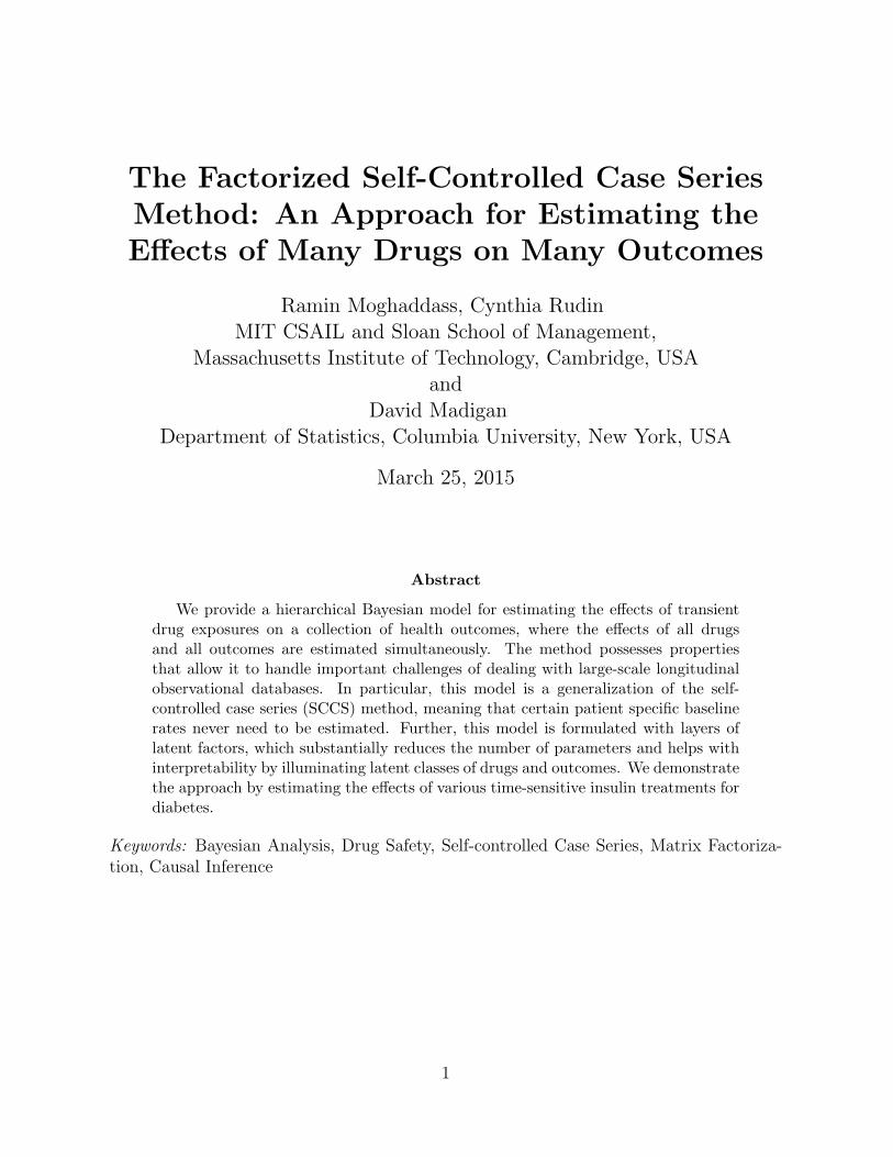
The Factorized Self-Controlled Case SeriesMethod: An Approach for Estimating theEffects of Many Drugs on Many Outcomes

Ramin Moghaddass, Cynthia RudinMIT CSAIL and Sloan School of Management,

Massachusetts Institute of Technology, Cambridge, USAand

David MadiganDepartment of Statistics, Columbia University, New York, USA

March 25, 2015

Abstract

We provide a hierarchical Bayesian model for estimating the effects of transientdrug exposures on a collection of health outcomes, where the effects of all drugsand all outcomes are estimated simultaneously. The method possesses propertiesthat allow it to handle important challenges of dealing with large-scale longitudinalobservational databases. In particular, this model is a generalization of the self-controlled case series (SCCS) method, meaning that certain patient specific baselinerates never need to be estimated. Further, this model is formulated with layers oflatent factors, which substantially reduces the number of parameters and helps withinterpretability by illuminating latent classes of drugs and outcomes. We demonstratethe approach by estimating the effects of various time-sensitive insulin treatments fordiabetes.

Keywords: Bayesian Analysis, Drug Safety, Self-controlled Case Series, Matrix Factoriza-tion, Causal Inference

1

1 Introduction

The medical community, the pharmaceutical industry, and health authorities are obligated

to confirm that marketed medical products and prescription drugs have acceptable benefit-

risk profiles; in fact, these entities have come under increasing scientific, regulatory and

public scrutiny to accurately estimate the effects of drugs. The increasing availability of

large-scale longitudinal observational healthcare databases (LODs) opens up exciting new

opportunities to add to the evidence base concerning these issues, though the complexity

and scale of some of the available databases presents interesting statistical and computa-

tional challenges. In what follows we focus on using longitudinal observational databases

to make inference about the effects of many drugs with respect to many outcomes simul-

taneously.

Many research studies have attempted to characterize the relationship between time-

varying drug exposures and adverse events (AEs) related to health outcomes (e.g., in Madi-

gan 2009, Greene et al. 2011, Chui et al. 2014, Benchimol et al. 2013, Simpson et al. 2013)

and the use of LODs to study individual drug-adverse effect combinations has become rou-

tine. The medical literature provides many examples and many different epidemiological

and statistical approaches, often tailored to the specific drug and specific adverse effect.

There is a major flaw in these approaches of estimating the effect of one drug on one

outcome, which is that it is very clear that many drugs are closely related to each other

(there are dozens of antibiotics for instance), and many heath outcomes are closely related

to each other (e.g., strokes, heart attacks, and other vascular diseases); we should leverage

this information to better understand causal effects. In this work, we borrow strength

across both drugs and outcomes in order to obtain better estimates for each individual

drug and outcome. Since we are interested in the causal effect of the drug, and not in

the patient-specific baseline rate of the outcome, we use the ideas of the self-controlled

case series (SCCS) method of Farrington (1995), which is a conditional Poisson regression

approach wherein each patient serves as his or her own control. The SCCS method has

been widely applied, especially in vaccine studies (see the tutorial of Whitaker et al. 2006).

SCCS controls for all fixed patient-level covariates but remains susceptible to time-varying

confounding. The standard SCCS method focuses on one drug and one outcome. Simp-

2

son et al. (2013) proposed the multiple self-controlled case series (MSCCS) method that

simultaneously provides effect estimates for multiple drugs and a single outcome. In fact,

the MSCCS provides a self-controlled approach that can control for many time-varying co-

variates, drugs being a special case. Bayesian implementations of both SCCS and MSCCS

provide significant advantages, especially in high-dimensional settings with thousands or

even tens of thousands of drugs and outcomes and even larger numbers of interactions.

Neither SCCS nor MSCCS account for the fact that many drugs/treatments naturally

form classes and therefore regression coefficients for drugs from within a single class might

reasonably be modeled as arising exchangeably from a common prior distribution. Adverse

events and health conditions can also be organized hierarchically, again affording an oppor-

tunity to “borrow strength” across related outcomes. For both drugs and outcomes, the

hierarchy could extend to multiple levels. In what follows we formalize these ideas within

the framework of latent factor Bayesian hierarchical models.

Factor models, which have been traditionally used in behavioral sciences, provide a flex-

ible framework for modeling multivariate data via unobserved latent factors (e.g., Ghosh &

Dunson 2009). In this paper, we do not impose specific latent structure a priori. However,

our approach can also be used for cases where classes of drugs and conditions are known a

priori. We will show that the latent factor approach not only brings more interpretability

to our model, but also can significantly contribute to reducing the computational complex-

ity. To our knowledge, only few works have considered matrix factorization-based data

analysis techniques for drug safety and surveillance (for example, Zitnik & Zupan 2015, for

drug-induced liver injury prediction and Cobanoglu et al. 2013, for predicting drug-target

interactions in neurobiological disorders, which are both very different than our study).

We introduce three models for predicting the effects of multiple drugs on multiple

outcomes that use hierarchical Bayesian analysis. The first model (Model 0) does not use

latent factors, and borrows strength across all drugs and outcomes. The second model

(Model 1) uses one set of latent drugs and one set of latent outcomes, through a single

matrix factorization. The third model (Model 2) uses two sets of latent factors, by factoring

the matrix of coefficients into three matrices; one for converting drugs to latent drugs,

another for converting outcomes to latent outcomes, and the third for modeling the effects

3

of latent drugs on latent outcomes. By allowing for latent factors, the second and third

models provide an increased level of interpretability, use fewer variables, and are thus more

computationally efficient to estimate.

The rest of this paper is organized as follows: In Sections 2, 3, 4, and 5 we describe the

model and the Bayesian inference procedure. In Section 6 the structure of the MCMC for

parameter estimation is illustrated. We then use a series of simulations in Section 7 to show

that we can recover the true generating parameters from data. Finally, we demonstrate the

approach in Section 8 for estimating the effects of various insulin treatments for diabetes.

Our proposed methodology has broader applicability beyond estimating the effects of drugs

considered in this paper.

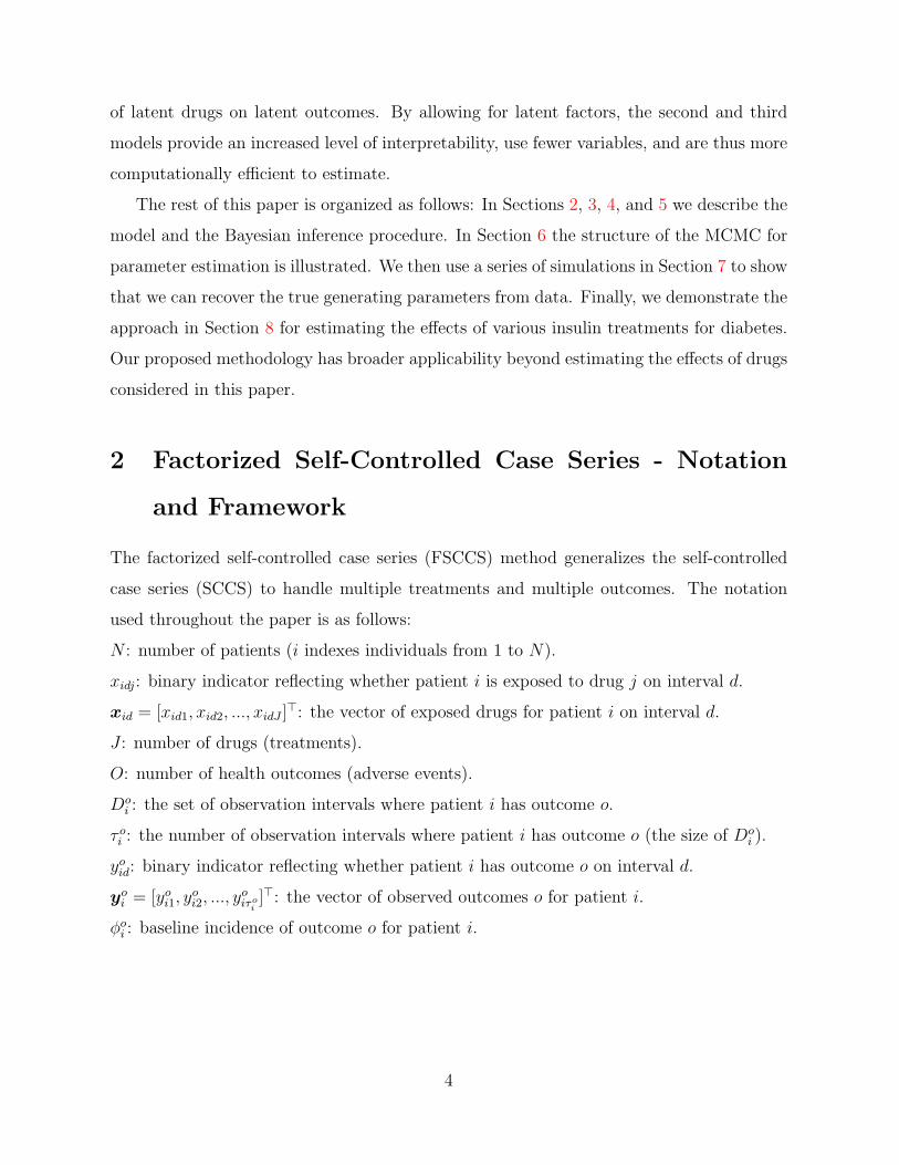
2 Factorized Self-Controlled Case Series - Notation

and Framework

The factorized self-controlled case series (FSCCS) method generalizes the self-controlled

case series (SCCS) to handle multiple treatments and multiple outcomes. The notation

used throughout the paper is as follows:

N : number of patients (i indexes individuals from 1 to N).

xidj: binary indicator reflecting whether patient i is exposed to drug j on interval d.

xid = [xid1, xid2, ..., xidJ ]⊤: the vector of exposed drugs for patient i on interval d.

J : number of drugs (treatments).

O: number of health outcomes (adverse events).

Doi : the set of observation intervals where patient i has outcome o.

τ oi : the number of observation intervals where patient i has outcome o (the size of Doi ).

yoid: binary indicator reflecting whether patient i has outcome o on interval d.

yoi = [yoi1, y

oi2, ..., y

oiτoi

]⊤: the vector of observed outcomes o for patient i.

ϕoi : baseline incidence of outcome o for patient i.

4

Φ =

ϕ11 ... ϕO

1

: : :

ϕ1N ... ϕO

N

: baseline incidence matrix.

βoj : regression coefficients associated with outcome o and drug j.

βo = [βo1 , β

o2 , ..., β

oJ ]

⊤: regression coefficients associated with outcome o.

B =

β11 ... βO

1

: : :

β1J ... βO

J

: drug-outcome coefficient matrix.

λ0id = exp(ϕo

i + x⊤idβ

o): the Poisson event rate of outcome o, for patient i, on interval d.

Outcomes occur according to a nonhomogeneous Poisson process, where drug exposure

can modulate the rate over time. Patient i has an individual baseline rate of exp(ϕoi ) for

outcome o that remains constant over time. Drug j has a multiplicative effect of exp(βoj )

on the individual baseline rate exp(ϕoi ) during its exposure period. The Poisson event rate

for outcome o and patient i on interval d according to the SCCS is:

λoid = exp(ϕo

i + x⊤idβ

o).

The key benefit of the SCCS is that the ϕoi terms do not need to be modeled, since we

are interested in the ratio of Poisson intensities with and without the drug. For instance,

considering only one drug j, comparing the intensity ratio for day d1 to a different day d2

with no exposure to the drug, we have:

λoid1

λoid2

=exp(ϕo

i + 1βoj )

exp(ϕoi + 0βo

j )= exp(βo

j ).

As the Poisson rate is assumed to be constant in each interval, the number of outcomes

o observed for patient i on interval d is distributed as a Poisson random variable (r.v.)

denoted by Y oid as

Pr(Y oid = yoid|xid) =

e−λoidλo

idyoid

yoid!.

Based on the above, the contribution to the likelihood for patient i and outcome o for the

observed sequence of events yoi = [yoi1, y

oi2, ..., y

oiτoi

]⊤, conditioned on the observed exposures

5

xi = [xi1, ...,xiτoi] is

L0i = Pr(yo

i |xi) =∏d∈Do

i

Pr(yoid|xid) = exp

−∑d∈Do

i

eϕoi+x⊤

idβo

∏d∈Do

i

(eϕ

oi+x⊤

idβo)yoid

yoid!(2.1)

= exp

−eϕoi

∑d∈Do

i

ex⊤idβ

o

∏d∈Do

i

eϕoi y

oid

∏d∈Do

i

(ex

⊤idβ

o)yoid

yoid!

= exp

ϕoin

oi − eϕ

oi

∑d∈Do

i

ex⊤idβ

o

∏d∈Do

i

(ex

⊤idβ

o)yoid

yoid!,

where noi =

∑d y

oid. It is assumed here that future outcomes are independent of past out-

comes and also outcomes are independent of each other. One could form the full likelihood

to estimate the unknown parameters (Φ,B). In order to avoid estimating the nuisance pa-

rameter set Φ, we can condition on its sufficient statistic, which removes the dependence on

Φ. The cumulative intensity is a sum (rather than an integral) since we assume a constant

intensity over each interval. Conditioning on noi yields the following likelihood for person

i:

Loi = Pr(yo

i |xi, noi ) =

∏d∈Do

i

Pr(yoid|xid)

Pr(noi |xi)

=

∏d∈Do

i

Pr(yoid|xid)exp

−∑

d∈Doi

λoid

∑d∈Do

i

λoid

noi

noi !

(2.2)

∝ exp∏d∈Do

i

ex⊤idβ

o∑d′ex

⊤id′β

o

yoid

.

Notice that because noi is sufficient, the individual likelihood in the above expression no

longer containsΦ. Assuming that patients are independent and conditions are independent,

the full conditional likelihood for event o is simply the product of the individual likelihoods

(i.e. Lo =N∏i=1

Loi ). Intuitively it follows that if i has no outcomes of type o, it cannot

provide any information about the relative rate of outcome o.

We now present three hierarchical models for multiple drug, multiple outcome self-

controlled case series and discuss how to estimate the drug-outcome coefficient matrix B.

6

Two of the models have latent factors that allow B to be expressed in a simpler and more

interpretable way. In our experiments, the empirical performance of these methods is about

the same.

3 Model 0 - No latent factors

Instead of estimating each coefficient independently, we borrow strength over both drugs

and outcomes, which adds substantial regularization. One should think of this as being

relevant for a set of related outcomes and drugs, e.g., heart-disease related outcomes and

the set of drugs one might prescribe for heart-related conditions. We shrink the estimates

for drug j over all outcomes to µj by placing an independent normal prior on each βoj

as βoj ∼ N (µj, σ

2j ),∀(j, o), where µj ∼ N (0, γ),∀j. We also assume uniform priors for

hyperparameters σj and γ as σj ∼ U(0, a), ∀j and γ ∼ U(0, a), where parameter a is a

user-defined constant. A natural extension of this model (not explored here) would be to

have drugs belong to certain classes of drugs, so that priors can be defined based on each

class of drugs; similarly with outcomes. The posterior probability of our model is now

defined as

Pr(B,µ,σ, γ|y, a) = Pr(y|B)× Pr(B|µ,σ)× Pr(µ|γ)× Pr(γ|a)× Pr(σ|a) (3.1)

∝∏o

∏i

∏d∈Di

(exp

(x⊤idβ

o)∑

d′ exp(x⊤id′β

o))y

(o)id

×∏j

∏o

N (βoj |µj, σ

2j ) ×

∏j

N (µj|0, γ)×∏j

Pr(σj|a)× Pr(γ|a).

The negative log-posterior (which can be used for finding the MAP solution if desired) is:

L1 = − log (Pr(B,µ,σ, γ|y, a)) .

The graphical representation of this model is shown in Figure 1.

7

..γ.

σj

.

µj

.

βoj

.a .

B

...

j = 1 : J

...

o = 1 : O

Figure 1: Graphical representation of Model 0

4 Model 1 - One level of latent factors

This model is motivated by two considerations. First, modeling the full posterior distri-

bution of Model 0 can be computationally expensive, particularly for large N , J , and O,

where J and O determine the number of variables to be estimated within the B matrix.

Second, Model 0 overlooks the fact that drugs and outcomes might come from a smaller

number of latent classes; for instance, there are commonly several drugs that are extremely

similar to each other for treating a set of highly related illnesses. We consider F latent

factors for drugs and outcomes. We model the J ×O matrix B as B = L(D) ×L(O), where

L(D) =

L

(D)1,1 ... L

(D)1,F

: : :

L(D)J,1 ... L

(D)J,F

,L(O) =

L(O)1,1 ... L

(O)1,O

: : :

L(O)F,1 ... L

(O)F,O

.

8

This way, we do not assume we know in advance which drugs have similar effects on which

outcomes, instead we estimate this from data. The number of latent factors F can be

determined by cross-validation. The total number of latent factors is J×F +F ×O, which

can be substantially less than J ×O.

For drug latent factors, we place independent normal priors on the entries of L(D) as

L(D)jf ∼ N (µ

(D)f , σ

(D)2f ),∀(j, f), where µ

(D)f ∼ N (0, γ(D)),∀f.

Similarly, we define normal priors on the entries of L(O) as

L(O)fo ∼ N (µ

(O)f , σ

(O)2f ),∀(f, o), where µ

(O)f ∼ N (0, γ(O)),∀f.

We assume uniform priors for hyperparameters σj and γ as σ(D)f ∼ U(0, a),∀f , σ(O)

f ∼

U(0, a),∀f , γ(D) ∼ U(0, b), γ(O) ∼ U(0, b), where (a, b) are known parameters. The poste-

rior probability is now defined as:

Pr(L(D),L(O),µ(D),µ(O),σ(D),σ(O), γ(D), γ(O)|y) = Pr(y|L(D),L(O)) (4.1)

× Pr(L(D)|µ(D),σ(D))× Pr(L(O)|µ(O),σ(O))× Pr(µ(D)|γ(D))× Pr(µO|γ(O))

× Pr(σ(D)|a)× Pr(σ(O)|a)× Pr(γ(D)|b)× Pr(γ(O)|b)

∝∏o

∏i

∏d∈Do

i

(exp

(x⊤idβ

o)∑

d′ exp(x⊤id′β

o))y

(o)id

×J∏

j=1

F∏f=1

N (L(D)jf |µ(D)

f , σ(D)2f )×

F∏f=1

(O)∏o=1

N (L(O)fo |µ(O)

f , σ(O)2f )

×F∏

f=1

N (µ(D)f |0, γ(D))×

F∏f=1

N (µ(O)f |0, γ(O))

× Pr(σ(D)f |b)× Pr(σ

(O)f )|b)× Pr(γ(D)|a)× Pr(γ(D)|a).

The graphical representation of this hierarchical Bayesian model is given in Figure 2.

5 Model 2 - Two levels of latent factors

Here we represent B as:

B = L(D) × L(F ) × L(O),

9

..b. a. a. b.

γ(D)

.

γ(O)

.

µ(D)f

.

µ(O)f

.

σ(D)f

.

σ(O)f

.

L(D)jf

.

L(O)fo

.

L(D)

.

L(O)

.

B

...

f = 1 : F

...

o

...

j

Figure 2: The Graphical Framework for Hierarchical Bayesian Model with one level of

latent factors

where

B =

L(D)1,1 ... L

(D)1,F1

: : :

L(D)J,1 ... L

(D)J,F1

×

L(F )1,1 ... L

(F )1,F2

: : :

L(F )F1,1

... L(F )F1,F2

×

L(O)1,1 ... L

(O)1,O

: : :

L(O)F2,1

... L(O)F2,O

.

The number of latent factors is thus J × F1 + F1 × F2 + F2 × O, which can be less than

the number of variables of Model 1 in many cases. Its major benefit is interpretability,

since now the number of latent drug factors and the number of latent outcome factors can

be estimated differently. L(D) represents the relationship between latent drugs and latent

10

drug-related factors, L(F ) represents the relationship between latent drug-related factors

and health outcome-related factors, and L(O) represents the relationship between drug-

related factors and health outcome-related factors. L(O) is really the core set of variables

since they relate the latent treatments to the latent outcomes. Note that latent factors

could be some known categories/classes of drugs and health conditions. The idea here is

to analyze all related drugs and related health events simultaneously.

The priors are L(D)jF1

∼ N (µ(D)F1

, σ(D)2F1

), L(O)F2o

∼ N (µ(O)F2

, σ(O)2F2

), L(F )F1F2

∼ N (µ(F ), σ(F )2),

µ(D)F1

∼ N (0, γ(D)), µ(F ) ∼ N (0, γ(F )), µ(O)F2

∼ N (0, γ(O)), σ(D)F1

∼ U(0, a), σ(F ) ∼ U(0, a),

σ(O)F2

∼ U(0, a), γ(D) ∼ U(0, b), γ(F ) ∼ U(0, b), and γ(O) ∼ U(0, b) for all (F1, F2, j, o).

The posterior probability is:

Pr(L(D),L(F ),L(O),µ(D),µ(F ),µ(O),σ(D),σ(F ),σ(O), γ(D), γ(F ), γ(O)|y) (5.1)

= Pr(y|L(D),L(F ),L(O))× Pr(L(D)|µ(D),σ(D))× Pr(L(F )|µ(F ),σ(D))× Pr(L(O)|µ(O),σ(O))

× Pr(µ(D)|γ(D))× Pr(µ(F )|γ(F ))× Pr(µ(O)|γ(O))

× Pr(σ(D)|a)× Pr(σ(F )|a)× Pr(σ(O)|a)× Pr(γ(D)|b)× Pr(γ(F )|b)× Pr(γ(O)|b).

Table 1 compares the number of parameters in each of the three models. Models 1 and

2 have much fewer parameters when F , F1, and F2 are lower than J and O.

Table 1: The number of parameters and hyperparameters in each model

Model Name # of Parameters # of Hyperparameters Total

Model 0 J ∗O 2 ∗ J + 1 J ∗O + 2 ∗ J + 1

Model 1 J ∗ F + F ∗O 4 ∗ F + 2 J ∗ F + F ∗O + 4 ∗ F + 2

Model 2 J ∗ F1 + F1 ∗ F2 + F2 ∗O 2 ∗ F1 + 2 ∗ F2 + 5 J ∗ F1 + F1 ∗ F2 + F2 ∗O + 2 ∗ F1 + 2 ∗ F2 + 5

6 Parameter Estimation Using Markov Chain Monte

Carlo

We use Markov Chain Monte Carlo (MCMC) to approximate the entries of B, specifically

random walk Metropolis (RWM). The algorithm employs a Gaussian proposal distribution

11

Jt(x, x′) which proposes a new parameter set x′ given the current parameter set x. We

denote Θ as the set of all parameters in the model excluding B.

Step 1. set t= 0. Generate an initial state {B0,Θ0} with positive probability Pr(B0,Θ0|y).

Repeat the following until stationary distribution and the desired number of samples are

reached considering optional burn-in and/or thinning.

Step 2. Sample {B∗,Θ∗} from the symmetric proposal distribution Jt({B0,Θ0},. ).

Step 3. Calculate the acceptance probability

α = min

(1,

Pr(B∗,Θ∗|y)Pr(Bt−1,Θt−1|y)

).

Step 4. Draw a random number u from Unif(0, 1). If u ≤ α, accept the proposal state

{B∗,Θ∗} and set Bt = B∗,Θt = Θ∗, else set Bt = Bt−1,Θt = Θt−1. Set t : t+ 1.

Our implementation uses a component-wise sampling approach, that is, when a sample

for one dimension is proposed, all other dimensions are held fixed. After the current sample

get accepted or rejected, we then move on to the next dimension and repeat the process

while holding all other dimensions constant. For truly large-scale applications, blocked

sampling approaches may be necessary.

7 Simulation Study

We will show that for data generated from our model, the true data-generating parameters

B can be recovered. We simulated sample trajectories of drug exposure and health outcomes

for 600 patients over 60 days. We set the number of drugs to J = 4, and the number of

health conditions to O = 4. Each patient randomly took between 1− J drugs over the 60

days. The average exposure period was assumed to be 20% of the study interval for each

patient (that is, on average, each patient was exposed to one or more drugs for at least 12

days). The exposure intervals are randomly selected, so these intervals could be multiple

non-consecutive days, multiple consecutive days, or a combination of both. Drugs can have

positive or negative contributions to the likelihood and intensity rate of each outcome. For

each model (Model 0, Model 1, Model 2), we generated the elements of B according to the

model’s hierarchy. Figure 3 and Figures 12-13 (which are given in the Appendix) show the

posterior density for each parameter of B, for Models 0, 1 and 2, as estimated by MCMC

12

sampling. These figures show that the posterior samples were concentrated around the true

values and the posterior mean of each variable was generally close to its true value. We

β1,1

-2.6 -2.4 -2.20

0.2

0.4

β1,2

-1.3 -1.2 -1.10

0.2

0.4

β1,3

-2 -1.8 -1.60

0.2

0.4

β1,4

-2.5 -2 -1.50

0.2

0.4

β2,1

1.15 1.2 1.250

0.2

0.4

β2,2

0.6 0.7 0.80

0.2

0.4

β2,3

0.6 0.7 0.80

0.2

0.4

β2,4

1.5 1.6 1.70

0.2

0.4

β3,1

1.6 1.65 1.7

Post

erio

r de

nsity

0

0.2

0.4

β3,2

1.6 1.65 1.70

0.2

0.4

β3,3

0.8 0.9 10

0.2

0.4

β3,4

-1 -0.9 -0.80

0.2

0.4

β4,1

-0.6 -0.5 -0.40

0.2

0.4

β4,2

0.3 0.4 0.50

0.2

0.4

β4,3

-1 -0.8 -0.60

0.2

0.4

β4,4

-0.3 -0.2 -0.10

0.2

0.4

Figure 3: Normalized histograms of posterior samples for each element of B in Model 0.

The vertical line indicates the true value.

summarize Figures 3, 12, and 13 in Figure 4, which provides a scatter plot of the posterior

means and true values for each of the three models. It can be observed that each of the

posterior means are very close to their true values.

8 Application to Blood Glucose Analysis for Diabetes

We consider an application to Insulin-Dependent Diabetes Mellitus, where our goal is to

predict blood glucose level outcomes under different circumstances of a patient’s daily life,

including their recent eating history, exercise, and insulin injections. Our data are longi-

tudinal measurements taken multiple times per day from 70 patients (this is the AIM-94

data set provided by Michael Kahn, MD, PhD, Washington University, St. Louis, MO,

13

True values-2.6 -1.6 -0.6 0.4 1.4

Post

erio

r m

ean

-2.6

-1.6

-0.6

0.4

1.4

2a) Model 0

True values-1.2 -0.8 -0.4 0

Post

erio

r m

ean

-1.2

-0.8

-0.4

0

b) Model 1

True values-1.5 -1 -0.5 0 0.5

Post

erio

r m

ean

-1.5

-1

-0.5

0

0.5

c) Model 2

Figure 4: Scatter plot of posterior means vs. true parameter values of elements of B for

Models 0, 1 and 2.

Bache & Lichman 2013). We aim mainly to illustrate (i) how the models we introduce

can be used with complex longitudinal data to predict outcomes, (ii) the prediction power

and (iii) interpretability of the proposed models. It is well known that current therapies

for regulating glucose level in diabetics are very challenging and often frustrating, as they

require patients to continuously regulate diet, exercise and various medications – any de-

viations can be dangerous (Benchimol et al. 2013). Our dataset and code will be made

publicly available for the purpose of reproducibility. Blood glucose measurements, symp-

toms and insulin treatments were recorded with timestamps for each patient, over the

course of several weeks to months.

The two main classes of health outcomes considered here are hyperglycemia (high blood

glucose) and hypoglycemia (low blood glucose). All other health outcomes we define later

are related to these two classes. Figure 5 provides a schematic of the type of data we are

considering for one patient over a course of day. We will describe the setup in more detail:

Drugs/Treatments: Diet, exercise, and injected insulin were treated as three different

classes of treatments. It is obvious that interactions among these treatments are important.

Insulin doses are given one or more times a day, typically before meals and sometimes also

at bedtime. Three types of insulin were considered: (1) regular, (2) Neutral Protamine

Hagedorn (NPH), and (3) Ultralente. Each insulin type has its own characteristic time of

onset (O), time of peak action (P), and effective duration (D). The exposure time intervals

14

Time 6:00 8:00 10:00 12:00 14:00 16:00 18:00 20:00 22:00

More-than-usualexercise activity

Less-than-usualmeal ingestion NPH injection

Pre-lunch BG measurement

(60 mg/dl)

Pre-lunch BG measurement

(47 mg/dl)

NPH injection

Pre-breakfast BGmeasurement(135 mg/dl)

Pre-snack BGmeasurement(118 mg/dl)

Measurements

Events

Figure 5: Sample longitudinal traces for a patient with multiple drug/treatments exposures

and blood Glucose measurements over a day. Downwards arrows indicate only measure-

ments. Upwards arrows indicate treatments.

for peak, and duration used in this paper, which were provided with the dataset, are shown

in Table 2 in the “Exposure Time” column in the bottom several rows of the table labeled

“Insulin.”

Based on the actual time of injection, we determined the intervals at which the patient

is at peak and/or within the duration of an insulin injection. Based on this, six types of

treatments were considered, (1) regular insulin on peak, (2) regular insulin on duration, (3)

NPH insulin on peak, (4) NPH insulin on duration, (5) Ultralente insulin on peak, and (6)

Ultralente insulin on duration. At each interval of time, the patient can be either insulin

free or subject to one of the above six exposures.

The second class of treatment is for exercise, which may have complex effects on glu-

cose level. For example, glucose levels can fall during exercise but also quite a few hours

afterwards. Three types of exercise are reported, (1) normal exercise, (2) lower than nor-

mal exercise, and (3) higher than normal exercise. Each type of exercise was considered

separately as a single treatment.

The third class of treatment is for diet, which also can have complex effects on the

glucose level. For example, a larger meal may lead to a longer and possibly higher elevation

15

Table 2: The list of drugs/treatments and health outcomes and their known correlations.

P means strong positive correlation, and N means strong negative correlation, D1 is lower

decile and D10 means highest decile.

TreatmentExposure

Time

Health Outcome

Low Glucose Level High Glucose Level

1. Too low 2. Low 3. D1 4. Hypo Symptom 5. Too High 6. High 7. D10

Exercise

1. Normal 0-4 h − − − − − − −

2. Too High 0-4 h P P P P N N N

3. Low 0-4 h − − − − − − −

Diet

Level

4. Normal 0-4 h − − − − − − −

5. Too High 0-4 h N N N N N N N

6. Low 0-4 h − − − − − − −

Time7. After Meal 0-4 h N N N N P P P

8. Before Meal 0-4 h P P P P N N N

Insulin

Regular9. Peak 1-3 h P P P P N N N

10. Duration 0-5 h P P P P N N N

NPH11. Peak 4-6 h P P P P N N N

12. Duration 0-12 h P P P P N N N

Ultralente13. Peak 14-24 h P P P P N N N

14. Duration 0-27 h P P P P N N N

of blood glucose. Missing a meal may put the patient at risk for low glucose levels in the

hours that follow. Three types of diet are reported: (1) normal diet, (2) higher than normal

diet, and (3) lower than normal diet. Each of these types of diet were taken as a single

treatment. Since measurements were collected before a meal, after a meal, and at other

times, we considered two other features in the model, (1) before meal measurement of blood

glucose and (2) after meal measurement, and we treated them as binary features. These

extra features allow us to distinguish whether the measurement was made before or after

the meal (there is a big difference between glucose measurements taken before a meal and

after a meal).

Based on all of the treatments described, the total number of variables associated with

treatments in the model is 14 (J = 14). The variables are all listed on Table 2 in the

“Treatment” column on the left.

Health Outcomes. The outcomes are divided into two major categories, i) high glucose

16

level and ii) low glucose level. Given that normal pre-meal blood glucose ranges from

approximately 80-120 mg, and post-meal blood glucose ranges from 80-140 mg/dl (Bache

& Lichman 2013), we considered seven health outcomes for glucose level: extremely low

(below 40 mg/dl), low (between 40-80 mg/dl), high (over 140 mg/dl), extremely high (over

180 mg/dl), lower decile (lower 10% of glucose level for each patient), upper decile (upper

10% of glucose level for each patient), and hypoglycemic (low glucose) symptoms. Thus,

the total number of outcomes considered for our analysis is O = 7. We can perform an

evaluation only on intervals where we have glucose measurements, thus we only use those

intervals.

True Relationships Between Drugs and Outcomes. We wanted to determine

whether our model reproduces known relationships between treatments and glucose levels,

even though it was not explicitly designed to do so. The information about true relation-

ships within Table 2 come from material accompanying the dataset and www.diabetes.org.

We denoted known positive effects in Table 2 by P , strong negative effects by N , and

relationships that were unknown were denoted by dashes “–”. For example, we expect

NPH injection on peak to decrease the likelihood of having “Too High” glucose level, so

the correlation between NPH on peak and “Too High” glucose level is negative (N ).

Mixing. We performed cross-validation, dividing our data into five folds, each with the

same number of patients, training our models on four folds and testing on the fifth. We

removed the first 5000 iterations (as burn-in) of Metropolis-Hastings sampling, and ob-

tained 6000 additional samples to estimate the posterior. Figure 6 shows samples from the

posterior of one of the variables, βToo high GLNPHonpeak , for five separate model instantiations (Model

0, Model 1 with F=2, Model 1 with F=3, Model 2 with F1 = 2, F2 = 2, and Model 2

with F1 = 3, F2 = 3. Recall that in Models 1 and 2, we sample elements of the matrices

of latent factors and then calculate B. From this figure, we observe reasonable mixing for

all models, and we observe that models with latent factors (Models 1 and 2) have better

mixing and convergence, possibly due to the smaller number of variables.

Computation. The number of parameters differs substantially between models, which

affects CPU time of the MCMC sampler. In Figure 7, the number of parameters for each

model and the associated CPU time for running MCMC are shown. This figure shows a

17

5000 20000 30000 40000 50000

Mod

el 0

-0.3-0.2-0.1

0

-0.25 -0.2 -0.15 -0.1 -0.05 00

500

1000

5000 2000 30000 4000 50000

Mod

el 1

F

=2

-0.3-0.2-0.1

0

-0.25 -0.2 -0.15 -0.1 -0.05 00

500

1000

5000 20000 30000 40000 50000

Mod

el 1

F

=3

-0.3-0.2-0.1

0

-0.25 -0.2 -0.15 -0.1 -0.05 00

500

1000

5000 20000 30000 40000 50000

M

odel

2

F

1=2,

F2=

2

-0.3-0.2-0.1

0

-0.2 -0.15 -0.1 -0.05 00

500

1000

Iteration No.5000 20000 30000 40000 50000

M

odel

2

F

1=3,

F2=

3

-0.3-0.2-0.1

0

-0.25 -0.2 -0.15 -0.1 -0.05 00

500

1000

Figure 6: Samples from the posterior of βToo high GLNPH on peak for five model instantiations (left), and

their histograms (right). The first 5000 samples were discarded as burn-in. We observe

better mixing and convergence in the models with latent factors (Model 1 and Model 2).

clear correlation between the number of variables and CPU time, that is CPU time increases

with the number of parameters. In particular, Model 0 takes a long time to run, because it

has substantially more variables than the other models. Interestingly, it seems that using

latent factors has a purpose beyond interpretability and regularization, in particular, it

helps substantially with tractability.

Interpretation of coefficients in B and comparison with ground truth. We

compare the estimated coefficients in B to the ground truth signs of coefficients given in

Table 2. It is not necessarily the case that the signs of the estimated coefficients need

to agree with the ground truth signs in order for the model to perform well, but it is a

reasonable aspect of the model to consider. To perform this comparison, we ranked the

estimated coefficients in B and used these rankings and the true signs of coefficients to

generate an ROC curve. That is, the ROC curve was generated by placing thresholds at

each point in the ranking, and calculating the true positive rate and false positive rate

with respect to the true coefficients. We computed these ROC curves for all five model

18

Number of parameters40 60 80 100 120 140

CPU

tim

e (h

ours

)

1.5

2

2.5

3

3.5

4

4.5

5

5.5

6

Model 1F=3

Model 2F

1=2, F

2=2

Model 2F

1=3, F

2=3

Model 1F=2

Model 0

Figure 7: Comparison between the CPU time and number of variables in the five model

instantiations. Model 0 has larger number of variables and significantly higher CPU time.

instantiations to obtain Figure 8. These ROC curves indicate that all models performed

well, in the sense of estimating reasonable signs for the coefficients, and also indicates that

models with more latent factors performed better than Model 0. The models with two

latent treatment and outcome factors performed slightly better than the models with three

latent treatment and outcome latent factors, though there was no significant difference in

performance between Model 1 and Model 2 for the same number of latent treatment and

outcome factors.

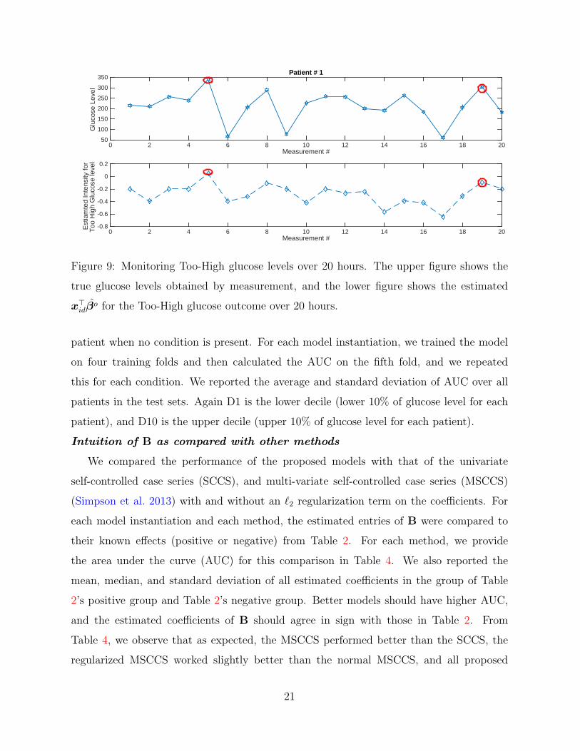
Drug Surveillance. We evaluated prediction performance of our model as follows: for

each patient we calculated the Poisson rate of each condition at each hour considering all

drug exposures. We then checked whether or not the patient had that condition at that

time. The Poisson rate acts as the score of each patient with regards to each condition. In

Figure 9, we present the actual glucose level for a patient at 20 measurement points (upper

figure) as well as the estimated intensity rate of the Too-High glucose level for the same

patient (lower figure). Each point in this figure represents the estimated x⊤idβ̂

o, where β̂o

are the estimated regression coefficients associated with too-high glucose level and x⊤id is the

known vector of drug exposures at interval d. The figure shows that the estimated intensity

rate is reasonably close to the actual level of glucose, particularly when the glucose level is

actually too high. In Figure 10, we repeated the analysis for Too-Low glucose level. It can

19

Specificity0 0.5 1

Sen

sitiv

ity

0

0.1

0.2

0.3

0.4

0.5

0.6

0.7

0.8

0.9

1Model 0

Specificity0 0.5 1

Sen

sitiv

ity

0

0.1

0.2

0.3

0.4

0.5

0.6

0.7

0.8

0.9

1Model 1, F=2

Specificity0 0.5 1

Sen

sitiv

ity

0

0.1

0.2

0.3

0.4

0.5

0.6

0.7

0.8

0.9

1Model 1, F=3

Specificity0 0.5 1

Sen

sitiv

ity

0

0.1

0.2

0.3

0.4

0.5

0.6

0.7

0.8

0.9

1Model 2, F

1=2, F

2=2

Specificity0 0.5 1

Sen

sitiv

ity

0

0.1

0.2

0.3

0.4

0.5

0.6

0.7

0.8

0.9

1Model 2, F

1=3, F

2=3

AUC=80% AUC=85% AUC=82% AUC=85% AUC=83%

Figure 8: Receiver Operating Characteristic (curve) for evaluating the signs of coefficients

against true signs for five model instantiations. See the text for details of how these curves

were generated.

be observed from this figure that the times where this coefficient is particularly large are the

same times where the glucose level drops substantially. This kind of dramatic agreement

was not observed for all patients nor all conditions, so below we describe a more general

evaluation procedure.

In Figure 11, we show the box plots for the estimated Poisson rates of the two conditions

of “Too Low” glucose level and “Too High” glucose level on all seventy patients in the test

sets. For comparison, we also plotted the box plots of the estimated Poisson rates for

normal conditions, where patients did not have too-high or too-low glucose levels. For

clarity and fairness, we normalized the estimated Poisson rates for each patient. It can be

observed from this figure that the estimated Poisson rate of these conditions are elevated

when patients actually suffer from Too-Low (or Too-High, respectively) glucose. Thus, our

model could be a useful approach for monitoring the likelihood of a condition, given the

timing of the drugs recently taken by the patient. The results were consistent across all

five model instantiations.

In Table 3, we report an AUC (area under the ROC curve) value that measures the

probability that a method ranks a positive condition timepoint higher than a timepoint

with no condition, for the same patient. In particular, we are testing whether the Poisson

rate of a patient with a health condition is higher than the estimated rate of the same

20

Measurement #0 2 4 6 8 10 12 14 16 18 20

Glu

cose

Lev

el

50

100

150

200

250

300

350Patient # 1

Measurement #0 2 4 6 8 10 12 14 16 18 20

Est

iam

ted

Inte

nsity

for

Too

Hig

h G

luco

se le

vel

-0.8

-0.6

-0.4

-0.2

0

0.2

Figure 9: Monitoring Too-High glucose levels over 20 hours. The upper figure shows the

true glucose levels obtained by measurement, and the lower figure shows the estimated

x⊤idβ̂

o for the Too-High glucose outcome over 20 hours.

patient when no condition is present. For each model instantiation, we trained the model

on four training folds and then calculated the AUC on the fifth fold, and we repeated

this for each condition. We reported the average and standard deviation of AUC over all

patients in the test sets. Again D1 is the lower decile (lower 10% of glucose level for each

patient), and D10 is the upper decile (upper 10% of glucose level for each patient).

Intuition of B as compared with other methods

We compared the performance of the proposed models with that of the univariate

self-controlled case series (SCCS), and multi-variate self-controlled case series (MSCCS)

(Simpson et al. 2013) with and without an ℓ2 regularization term on the coefficients. For

each model instantiation and each method, the estimated entries of B were compared to

their known effects (positive or negative) from Table 2. For each method, we provide

the area under the curve (AUC) for this comparison in Table 4. We also reported the

mean, median, and standard deviation of all estimated coefficients in the group of Table

2’s positive group and Table 2’s negative group. Better models should have higher AUC,

and the estimated coefficients of B should agree in sign with those in Table 2. From

Table 4, we observe that as expected, the MSCCS performed better than the SCCS, the

regularized MSCCS worked slightly better than the normal MSCCS, and all proposed

21

Measurement #0 2 4 6 8 10 12 14 16 18 20

Glu

cose

Lev

el

0

50

100

150

200

250Patient # 1

Measurement #0 2 4 6 8 10 12 14 16 18 20

Est

imat

ed In

tens

ity

Too

low

Glu

cose

Lev

el

-2

-1.5

-1

-0.5

0

0.5

1

Figure 10: Monitoring too-low glucose levels over 20 hours. The upper figure shows the

true glucose levels obtained by measurement, and the lower figure shows the estimated

x⊤idβ̂

o for the too-low glucose outcome over 20 hours.

Bayesian model instantiations (Model 0-2) performed better than all of the traditional

models, yielding higher AUC’s and better agreement in the mean signs of coefficients;

further the standard deviations for the coefficient values were substantially lower. These

performance benefits come in addition to the other benefits of our approach discussed

earlier, including computational tractability and interpretability of the latent factors.

9 Concluding Remarks

The novel elements of this work are as follows. (1) We estimate the effects of many drugs

on many health outcomes simultaneously. Borrowing strength across similar drugs and

outcomes allows us to create better estimates across both drugs and outcomes. (2) We use

latent factors to encode latent classes of drugs and outcomes, to help with interpretability,

and to provide a major computational benefit. A computational benefit is also provided

by the SCCS’s framework, since we do not need to estimate the baseline rates of outcomes

for each patient. This approach is scalable to large longitudinal observational databases,

is generally applicable (also to problems beyond healthcare), and provides a level of inter-

pretability to physicians and patients that was not previously possible.

22

Normal Too Low

Nor

mal

ized

Rat

e

0

0.2

0.4

0.6

0.8

1Model 0

Normal Too High

Nor

mal

ized

Rat

e

0

0.2

0.4

0.6

0.8

1Model 0

Normal Too Low0

0.2

0.4

0.6

0.8

1Model 1, F=2

Normal Too High0

0.2

0.4

0.6

0.8

1Model 1, F=2

Normal Too Low0

0.2

0.4

0.6

0.8

1

Model 2, F1 = F

2 = 2

Normal Too High0

0.2

0.4

0.6

0.8

1

Model 2, F1 = F

2 = 2

Normal Too Low0

0.2

0.4

0.6

0.8

1Model 1, F=3

Normal Too High0

0.2

0.4

0.6

0.8

1Model 1, F=3

Normal Too High0

0.2

0.4

0.6

0.8

1

Model 2, F1 = F

2 = 3

Normal Too Low0

0.2

0.4

0.6

0.8

1

Model 2, F1 = F

2 = 3

Figure 11: Comparison between the box-plots for Too-High and Too-Low glucose level and

normal condition for all five model instantiations, where the Poisson rates were normalized

for each person.

Acknowledgement

We gratefully acknowledge funding from the Natural Science and Engineering Research

Council of Canada (NSERC) and the MIT Big Data Initiative.

References

Bache, K. & Lichman, M. (2013), ‘UCI machine learning repository, University of Califor-

nia, Irvine, School of Information and Computer Sciences, http://archive.ics.uci.edu/ml’.

Benchimol, E., Hawken, S., Kwong, J. & Wilson, K. (2013), ‘Safety and utilization

of influenza immunization in children with inflammatory bowel disease’, Pediatrics

131(6), 1811–1820.

Chui, C., Man, K., Cheng, C.-L., Chan, E., Lau, W., Cheng, V., Wong, D., Yang Kao,

Y.-H. & Wong, I. (2014), ‘An investigation of the potential association between retinal

23

Table 3: Average and standard deviation (sd) of AUC over 5 folds. The entities that were

ranked for each score are pairs of timepoints for a patient, where for one of the timepoints

the patient had a condition and for the other timepoint the patient did not have a condition.

The AUC was calculated as the fraction of pairs of times (the first time with the condition

and the second time without the condition) where the estimated rate was higher when the

patient had the condition vs. when the patient did not have the condition.

Too low Low Too high High D1 D10 Hypo Symptom

Model 0Mean 70.30% 62.92% 62.98% 61.26% 58.20% 56.39% 59.17%

sd 9.56% 2.79% 3.38% 2.70% 3.93% 3.51% 4.95%

Model 1, F = 2Mean 70.86% 62.70% 63.06% 61.58% 57.97% 56.05% 56.71%

sd 8.28% 2.47% 3.14% 2.11% 3.36% 3.04% 3.19%

Model 1, F = 3Mean 70.66% 62.68% 62.92% 61.51% 57.97% 56.35% 56.33%

sd 7.89% 2.52% 3.14% 2.12% 3.37% 2.90% 2.87%

Model 2, F1 = F2 = 2Mean 70.19% 62.71% 62.97% 61.44% 58.00% 55.91% 56.88%

sd 9.51% 2.43% 3.18% 2.13% 3.34% 3.06% 3.02%

Model 2, F1 = 3, F2 = 3Mean 70.07% 62.73% 62.99% 61.47% 58.05% 56.05% 56.68%

sd 9.52% 2.44% 3.16% 2.07% 3.31% 3.05% 2.79%

detachment and oral fluoroquinolones: A self-controlled case series study’, Journal of

Antimicrobial Chemotherapy 69(9), 2563–2567.

Cobanoglu, M., Liu, C., Hu, F., Oltvai, Z. & Bahar, I. (2013), ‘Predicting drug-target

interactions using probabilistic matrix factorization’, Journal of Chemical Information

and Modeling 53(12), 3399–3409.

Farrington, P. (1995), ‘Relative incidence estimation from case series for vaccine safety

evaluation’, Biometrics 51, 228–235.

Ghosh, J. & Dunson, D. (2009), ‘Default prior distributions and efficient posterior com-

putation in Bayesian factor analysis’, Journal of Computational and Graphical Statistics

18(2), 306–320.

Greene, S., Kulldorff, M., Yin, R., Yih, W., Lieu, T., Weintraub, E. & Lee, G. (2011), ‘Near

24

Table 4: Comparison with existing models

MeasureMethod

Model 0Mode1

F = 2

Model 1

F = 3

Model 2

F1 = 2, F2 = 2

Model 2

F1 = 3, F2 = 3SCCS MSCCS

Regularized

MSCCS

AUC 0.813 0.852 0.824 0.856 0.836 0.693 0.773 0.774

B−

Mean -0.190 -0.281 -0.276 -0.278 -0.282 -0.492 -0.663 -0.349

Median -0.077 -0.136 -0.143 -0.130 -0.141 -0.047 -0.122 -0.122

sd 0.353 0.417 0.410 0.422 0.424 2.362 2.462 0.640

B+

Mean 0.071 0.099 0.096 0.105 0.096 -0.552 -0.561 -0.023

Median 0.030 0.103 0.111 0.106 0.106 0.065 0.126 0.125

sd 0.368 0.369 0.385 0.368 0.378 3.158 3.149 0.771

real-time vaccine safety surveillance with partially accrued data’, Pharmacoepidemiology

and Drug Safety 20(6), 583–590.

Madigan, D. (2009), ‘The self-controlled case series: Recent developments’, 94(6), 1057–

1063.

Simpson, S., Madigan, D., Zorych, I., Schuemie, M., Ryan, P. & Suchard, M. (2013),

‘Multiple self-controlled case series for large-scale longitudinal observational databases’,

Biometrics 69(4), 893–902.

Whitaker, H. J., Farrington, C. P., Spiessens, B. & Musonda, P. (2006), ‘Tutorial in bio-

statistics: the self-controlled case series method’, Statistics in Medicine 25(10), 1768–

1797.

Zitnik, M. & Zupan, B. (2015), ‘Matrix factorization-based data fusion for drug-induced

liver injury prediction’, Systems Biomedicine pp. 16–22.

25

Appendix: Figures 12 and 13

β1,1

-0.9 -0.8 -0.70

0.2

0.4

β1,3

-1.2 -1 -0.80

0.2

0.4

β1,4

-0.8 -0.7 -0.60

0.2

0.4

β2,1

-1.2 -1 -0.8

Post

erio

r de

nsity

0

0.2

0.4

β2,2

-0.55 -0.5 -0.45 -0.40

0.2

0.4

β2,3

-1.2 -1 -0.80

0.2

0.4

β2,4

-1 -0.8 -0.60

0.2

0.4

β3,1

-0.4 -0.2 00

0.2

0.4

β3,2

0 0.1 0.20

0.2

0.4

β3,3

-0.6 -0.5 -0.40

0.2

0.4

β3,4

-0.3 -0.2 -0.10

0.2

0.4

β4,1

-1.1 -1 -0.90

0.2

0.4

β4,2

-0.6 -0.55 -0.5 -0.450

0.2

0.4

β4,3

-1.2 -1 -0.80

0.2

0.4

β4,4

-1 -0.9 -0.80

0.2

0.4

β1,1

-0.4 -0.35 -0.3 -0.250

0.1

0.2

0.3

Figure 12: Normalized histograms of posterior samples for each element of B in Model 1.

The vertical line indicates the true value.

26

β1,1

0.4 0.5 0.60

0.2

0.4

β1,3

-1.5 -1.4 -1.30

0.2

0.4

β1,4

-1 -0.9 -0.80

0.2

0.4

β2,1

0.5 0.6 0.7

Post

erio

r de

nsity

0

0.2

0.4

β2,2

-0.6 -0.55 -0.5 -0.450

0.2

0.4

β2,3

-0.9 -0.8 -0.70

0.2

0.4

β2,4

-0.5 -0.4 -0.30

0.2

0.4

β3,1

0.4 0.5 0.60

0.2

0.4

β3,2

-0.25 -0.2 -0.15 -0.10

0.2

0.4

β3,3

-0.4 -0.3 -0.20

0.2

0.4

β3,4

-0.2 -0.1 00

0.2

0.4

β4,1

-0.5 -0.4 -0.30

0.2

0.4

β4,2

0.25 0.3 0.350

0.2

0.4

β4,3

0.4 0.5 0.60

0.2

0.4

β4,4

0.1 0.2 0.30

0.2

0.4

β1,2

-1.2 -1.1 -1 -0.90

0.1

0.2

0.3

Figure 13: Normalized histograms of posterior samples for each element of B in Model 2.

The vertical line indicates the true value.

27