The evolution of eusociality - University of Washington
49
ANALYSIS The evolution of eusociality Martin A. Nowak 1 , Corina E. Tarnita 1 & Edward O. Wilson 2 Eusociality, in which some individuals reduce their own lifetime reproductive potential to raise the offspring of others, underlies the most advanced forms of social organization and the ecologically dominant role of social insects and humans. For the past four decades kin selection theory, based on the concept of inclusive fitness, has been the major theoretical attempt to explain the evolution of eusociality. Here we show the limitations of this approach. We argue that standard natural selection theory in the context of precise models of population structure represents a simpler and superior approach, allows the evaluation of multiple competing hypotheses, and provides an exact framework for interpreting empirical observations. F or most of the past half century, much of sociobiological theory has focused on the phenomenon called eusociality, where adult members are divided into reproductive and (par- tially) non-reproductive castes and the latter care for the young. How can genetically prescribed selfless behaviour arise by natural selection, which is seemingly its antithesis? This problem has vexed biologists since Darwin, who in The Origin of Species declared the paradox—in particular displayed by ants—to be the most important challenge to his theory. The solution offered by the master naturalist was to regard the sterile worker caste as a ‘‘well- flavoured vegetable’’, and the queen as the plant that produced it. Thus, he said, the whole colony is the unit of selection. Modern students of collateral altruism have followed Darwin in continuing to focus on ants, honeybees and other eusocial insects, because the colonies of most of their species are divided unambiguously into different castes. Moreover, eusociality is not a marginal pheno- menon in the living world. The biomass of ants alone composes more than half that of all insects and exceeds that of all terrestrial nonhuman vertebrates combined 1 . Humans, which can be loosely characterized as eusocial 2 , are dominant among the land vertebrates. The ‘super- organisms’ emerging from eusociality are often bizarre in their consti- tution, and represent a distinct level of biological organization (Fig. 1). Rise and fall of inclusive fitness theory For the past four decades, kin selection theory has had a profound effect on the interpretation of the genetic evolution of eusociality and, by extension, of social behaviour in general. The defining feature of kin selection theory is the concept of inclusive fitness. When evaluating an action, inclusive fitness is defined as the sum of the effect of this action on the actor’s own fitness and on the fitness of the recipient multiplied by the relatedness between actor and recipient, where ‘recipient’ refers to anyone whose fitness is modified by the action. The idea was first stated by J. B. S. Haldane in 1955, and a foundation of a full theory 3 was laid out by W. D. Hamilton in 1964. The pivotal idea expressed by both writers was formalized by Hamilton as the inequality R . c/b, meaning that cooperation is favoured by natural selection if relatedness is greater than the cost to benefit ratio. The relatedness parameter R was originally expressed as the fraction of the genes shared between the altruist and the recipient due to their com- mon descent, hence the likelihood the altruistic gene will be shared. For example, altruism will evolve if the benefit to a brother or sister is greater than two times the cost to the altruist (R 5 1/2) or eight times in the case of a first cousin (R 5 1/8). Due to its originality and seeming explanatory power, kin selection came to be widely accepted as a cornerstone of sociobiological theory. Yet it was not the concept itself in its abstract form that first earned favour, but the consequence suggested by Hamilton that came to be called the ‘‘haplodiploid hypothesis.’’ Haplodiploidy is the sex- determining mechanism in which fertilized eggs become females, and unfertilized eggs males. As a result, sisters are more closely related to one another (R 5 3/4) than daughters are to their mothers (R 5 1/2). Haplodiploidy happens to be the method of sex determination in the Hymenoptera, the order of ants, bees and wasps. Therefore, colonies of altruistic individuals might, due to kin selection, evolve more frequently in hymenopterans than in clades that have diplodiploid sex determination. In the 1960s and 1970s, almost all the clades known to have evolved eusociality were in the Hymenoptera. Thus the haplodiploid hypo- thesis seemed to be supported, at least at first. The belief that haplo- diploidy and eusociality are causally linked became standard textbook fare. The reasoning seemed compelling and even Newtonian in con- cept, travelling in logical steps from a general principle to a widely distributed evolutionary outcome 4,5 . It lent credence to a rapidly developing superstructure of sociobiological theory based on the pre- sumed key role of kin selection. By the 1990s, however, the haplodiploid hypothesis began to fail. The termites had never fitted this model of explanation. Then more eusocial species were discovered that use diplodiploid rather than haplodiploid sex determination. They included a species of platypo- did ambrosia beetles, several independent lines of Synalpheus sponge- dwelling shrimp (Fig. 2) and bathyergid mole rats. The association between haplodiploidy and eusociality fell below statistical signifi- cance. As a result the haplodiploid hypothesis was in time abandoned by researchers on social insects 6–8 . Although the failure of the hypothesis was not by itself considered fatal to inclusive fitness theory, additional kinds of evidence began to accumulate that were unfavourable to the basic idea that relatedness is a driving force for the emergence of eusociality. One is the rarity of eusociality in evolution, and its odd distribution through the Animal Kingdom. Vast numbers of living species, spread across the major taxonomic groups, use either haplodiploid sex determination or clonal reproduction, with the latter yielding the highest possible degree of pedigree relatedness, yet with only one major group, the gall-making aphids, known to have achieved eusociality. For example, among the 1 Program for Evolutionary Dynamics, Department of Mathematics, Department of Organismic and Evolutionary Biology, Harvard University, Cambridge, Massachusetts 02138, USA. 2 Museum of Comparative Zoology, Harvard University, Cambridge, Massachusetts 02138, USA. Vol 466j26 August 2010jdoi:10.1038/nature09205 1057 Macmillan Publishers Limited. All rights reserved ©2010
Transcript of The evolution of eusociality - University of Washington

ANALYSIS
The evolution of eusocialityMartin A. Nowak1, Corina E. Tarnita1 & Edward O. Wilson2
Eusociality, in which some individuals reduce their own lifetime reproductive potential to raise the offspring of others,underlies the most advanced forms of social organization and the ecologically dominant role of social insects and humans.For the past four decades kin selection theory, based on the concept of inclusive fitness, has been the major theoreticalattempt to explain the evolution of eusociality. Here we show the limitations of this approach. We argue that standardnatural selection theory in the context of precise models of population structure represents a simpler and superior approach,allows the evaluation of multiple competing hypotheses, and provides an exact framework for interpreting empiricalobservations.
For most of the past half century, much of sociobiologicaltheory has focused on the phenomenon called eusociality,where adult members are divided into reproductive and (par-tially) non-reproductive castes and the latter care for the
young. How can genetically prescribed selfless behaviour arise bynatural selection, which is seemingly its antithesis? This problemhas vexed biologists since Darwin, who in The Origin of Speciesdeclared the paradox—in particular displayed by ants—to be themost important challenge to his theory. The solution offered by themaster naturalist was to regard the sterile worker caste as a ‘‘well-flavoured vegetable’’, and the queen as the plant that produced it.Thus, he said, the whole colony is the unit of selection.
Modern students of collateral altruism have followed Darwin incontinuing to focus on ants, honeybees and other eusocial insects,because the colonies of most of their species are divided unambiguouslyinto different castes. Moreover, eusociality is not a marginal pheno-menon in the living world. The biomass of ants alone composes morethan half that of all insects and exceeds that of all terrestrial nonhumanvertebrates combined1. Humans, which can be loosely characterizedas eusocial2, are dominant among the land vertebrates. The ‘super-organisms’ emerging from eusociality are often bizarre in their consti-tution, and represent a distinct level of biological organization (Fig. 1).
Rise and fall of inclusive fitness theory
For the past four decades, kin selection theory has had a profoundeffect on the interpretation of the genetic evolution of eusocialityand, by extension, of social behaviour in general. The defining featureof kin selection theory is the concept of inclusive fitness. Whenevaluating an action, inclusive fitness is defined as the sum of theeffect of this action on the actor’s own fitness and on the fitness of therecipient multiplied by the relatedness between actor and recipient,where ‘recipient’ refers to anyone whose fitness is modified by theaction.
The idea was first stated by J. B. S. Haldane in 1955, and a foundationof a full theory3 was laid out by W. D. Hamilton in 1964. The pivotalidea expressed by both writers was formalized by Hamilton as theinequality R . c/b, meaning that cooperation is favoured by naturalselection if relatedness is greater than the cost to benefit ratio. Therelatedness parameter R was originally expressed as the fraction of thegenes shared between the altruist and the recipient due to their com-mon descent, hence the likelihood the altruistic gene will be shared. Forexample, altruism will evolve if the benefit to a brother or sister is
greater than two times the cost to the altruist (R 5 1/2) or eight timesin the case of a first cousin (R 5 1/8).
Due to its originality and seeming explanatory power, kin selectioncame to be widely accepted as a cornerstone of sociobiological theory.Yet it was not the concept itself in its abstract form that first earnedfavour, but the consequence suggested by Hamilton that came tobe called the ‘‘haplodiploid hypothesis.’’ Haplodiploidy is the sex-determining mechanism in which fertilized eggs become females, andunfertilized eggs males. As a result, sisters are more closely related toone another (R 5 3/4) than daughters are to their mothers (R 5 1/2).Haplodiploidy happens to be the method of sex determination in theHymenoptera, the order of ants, bees and wasps. Therefore, coloniesof altruistic individuals might, due to kin selection, evolve morefrequently in hymenopterans than in clades that have diplodiploidsex determination.
In the 1960s and 1970s, almost all the clades known to have evolvedeusociality were in the Hymenoptera. Thus the haplodiploid hypo-thesis seemed to be supported, at least at first. The belief that haplo-diploidy and eusociality are causally linked became standard textbookfare. The reasoning seemed compelling and even Newtonian in con-cept, travelling in logical steps from a general principle to a widelydistributed evolutionary outcome4,5. It lent credence to a rapidlydeveloping superstructure of sociobiological theory based on the pre-sumed key role of kin selection.
By the 1990s, however, the haplodiploid hypothesis began to fail.The termites had never fitted this model of explanation. Then moreeusocial species were discovered that use diplodiploid rather thanhaplodiploid sex determination. They included a species of platypo-did ambrosia beetles, several independent lines of Synalpheus sponge-dwelling shrimp (Fig. 2) and bathyergid mole rats. The associationbetween haplodiploidy and eusociality fell below statistical signifi-cance. As a result the haplodiploid hypothesis was in time abandonedby researchers on social insects6–8.
Although the failure of the hypothesis was not by itself consideredfatal to inclusive fitness theory, additional kinds of evidence began toaccumulate that were unfavourable to the basic idea that relatedness isa driving force for the emergence of eusociality. One is the rarity ofeusociality in evolution, and its odd distribution through the AnimalKingdom. Vast numbers of living species, spread across the majortaxonomic groups, use either haplodiploid sex determination or clonalreproduction, with the latter yielding the highest possible degree ofpedigree relatedness, yet with only one major group, the gall-makingaphids, known to have achieved eusociality. For example, among the
1Program for Evolutionary Dynamics, Department of Mathematics, Department of Organismic and Evolutionary Biology, Harvard University, Cambridge, Massachusetts 02138, USA.2Museum of Comparative Zoology, Harvard University, Cambridge, Massachusetts 02138, USA.
Vol 466j26 August 2010jdoi:10.1038/nature09205
1057Macmillan Publishers Limited. All rights reserved©2010

70,000 or so known parasitoid and other apocritan Hymenoptera, allof which are haplodiploid, no eusocial species has been found. Nor hasa single example come to light from among the 4,000 known hymeno-pteran sawflies and horntails, even though their larvae often formdense, cooperative aggregations6,9.
It has further turned out that selection forces exist in groups thatdiminish the advantage of close collateral kinship. They include thefavouring of raised genetic variability by colony-level selection in theants Pogonomyrmex occidentalis10 and Acromyrmex echinatior11—due, at least in the latter, to disease resistance. The contribution ofgenetic diversity to disease resistance at the colony level has moreoverbeen established definitively in honeybees. Countervailing forcesalso include variability in predisposition to worker sub-castes inPogonomyrmex badius, which may sharpen division of labour andimprove colony fitness—although that hypothesis is yet to betested12. Further, an increase in stability of nest temperature withgenetic diversity has been found within nests of honeybees13 andFormica ants14. Other selection forces working against the bindingrole of close pedigree kinship are the disruptive impact of nepotismwithin colonies, and the overall negative effects associated withinbreeding15. Most of these countervailing forces act through group
selection or, for eusocial insects in particular, through between-colony selection.
During its long history, inclusive fitness theory has stimulatedcountless measures of pedigree kinship and made them routine insociobiology. It has supplied hypothetical explanations of phenomenasuch as the perturbations of colony investment ratios in male andfemale reproductives, and conflict and resolution of conflict amongcolony members. It has stimulated many correlative studies in the fieldand laboratory that indirectly suggest the influence of kin selection.
Yet, considering its position for four decades as the dominantparadigm in the theoretical study of eusociality, the production ofinclusive fitness theory must be considered meagre. During the sameperiod, in contrast, empirical research on eusocial organisms hasflourished, revealing the rich details of caste, communication, colonylife cycles, and other phenomena at both the individual- and colony-selection levels. In some cases social behaviour has been causallylinked through all the levels of biological organization from moleculeto ecosystem. Almost none of this progress has been stimulated oradvanced by inclusive fitness theory, which has evolved into anabstract enterprise largely on its own16.
Limitations of inclusive fitness theory
Many empiricists, who measure genetic relatedness and use inclusivefitness arguments, think that they are placing their considerations on
Figure 1 | The ultimate superorganisms. The gigantic queens of theleafcutter ants, one of whom (upper panel) is shown here, attended by someof her millions of daughter workers. Differences in size and labourspecialization allows the ants to cut and gather leaf fragments (middlepanel), and convert the fragments into gardens to grow fungi (lower panel).The species shown are respectively, top to bottom, Atta vollenweideri, Attasexdens and Atta cephalotes. (Photos by Bert Holldobler.)
a
c
b
Figure 2 | Species on either side of the eusociality threshold. a, A colony ofa primitively eusocial Synalpheus snapping shrimp, occupying a cavityexcavated in a sponge. The large queen (reproductive member) is supportedby her family of workers, one of whom guards the nest entrance (fromDuffy59). b, A colony of the primitively eusocial halictid bee Lasioglossumduplex, which has excavated a nest in the soil (from Sakagami andHayashida60). c, Adult erotylid beetles of the genus Pselaphacus leading theirlarvae to fungal food (from Costa9); this level of parental care is widespreadamong insects and other arthropods, but has never been known to give riseto eusociality. These three examples illustrate the principle that the origin ofeusociality requires the pre-adaptation of a constructed and guarded nestsite.
ANALYSIS NATUREjVol 466j26 August 2010
1058Macmillan Publishers Limited. All rights reserved©2010

a solid theoretical foundation. This is not the case. Inclusive fitnesstheory is a particular mathematical approach that has many limita-tions. It is not a general theory of evolution. It does not describeevolutionary dynamics nor distributions of gene frequencies17–19.But one of the questions that can be addressed by inclusive fitnesstheory is the following: which of two strategies is more abundant onaverage in the stationary distribution of an evolutionary process?Here we show that even for studying this particular question, theuse of inclusive fitness requires stringent assumptions, which areunlikely to be fulfilled by any given empirical system.
In the Supplementary Information (Part A) we outline a generalmathematical approach based on standard natural selection theory toderive a condition for one behavioural strategy to be favoured overanother. This condition holds for any mutation rate and any intensityof selection. Then we move to the limit of weak selection, which isrequired by inclusive fitness theory17,20–22. Here all individuals haveapproximately the same fitness and both strategies are roughlyequally abundant. For weak selection, we derive the general answerprovided by standard natural selection theory, and we show thatfurther limiting assumptions are needed for inclusive fitness theoryto be formulated in an exact manner.
First, for inclusive fitness theory all interactions must be additiveand pairwise. This limitation excludes most evolutionary games thathave synergistic effects or where more than two players areinvolved23. Many tasks in an insect colony, for example, require thesimultaneous cooperation of more than two individuals, and syn-ergistic effects are easily demonstrated.
Second, inclusive fitness theory can only deal with very specialpopulation structures. It can describe either static structures ordynamic ones, but in the latter case there must be global updatingand binary interactions. Global updating means that any two indivi-duals compete uniformly for reproduction regardless of their (spatial)distance. Binary interaction means that any two individuals eitherinteract or they do not, but there cannot be continuously varyingintensities of interaction.
These particular mathematical assumptions, which are easily vio-lated in nature, are needed for the formulation of inclusive fitnesstheory. If these assumptions do not hold, then inclusive fitness eithercannot be defined or does not give the right criterion for what isfavoured by natural selection.
We also prove the following result: if we are in the limited worldwhere inclusive fitness theory works, then the inclusive fitness con-dition is identical to the condition derived by standard natural selec-tion theory. The exercise of calculating inclusive fitness does notprovide any additional biological insight. Inclusive fitness is justanother way of accounting3,20,24, but one that is less general (Fig. 3).
The question arises: if we have a theory that works for all cases(standard natural selection theory) and a theory that works only for asmall subset of cases (inclusive fitness theory), and if for this subsetthe two theories lead to identical conditions, then why not stay withthe general theory? The question is pressing, because inclusive fitnesstheory is provably correct only for a small (non-generic) subset ofevolutionary models, but the intuition it provides is mistakenlyembraced as generally correct25.
Sometimes it is argued that inclusive fitness considerations pro-vide an intuitive guidance for understanding empirical data in theabsence of an actual model of population genetics. However, as weshow in the online material, inclusive fitness arguments without afully specified model are misleading. It is possible to consider situa-tions where all measures of relatedness are identical, yet cooperationis favoured in one case, but not in the other. Conversely, two popula-tions can have relatedness measures on the opposite ends of thespectrum and yet both structures are equally unable to supportevolution of cooperation. Hence, relatedness measurements withouta meaningful theory are difficult to interpret.
Another commonly held misconception is that inclusive fitnesscalculations are simpler than the standard approach. This is not
the case; wherever inclusive fitness works, the two theories are ident-ical and require the measurement of the same quantities. The impres-sion that inclusive fitness is simpler arises from a misunderstandingof which effects are relevant: the inclusive fitness formula contains allindividuals whose fitness is affected by an action, not only thosewhose payoff is changed (Fig. 3c).
Hamilton’s rule almost never holdsInclusive fitness theory often attempts to derive Hamilton’s rule, butfinds it increasingly difficult to do so. In a simplified Prisoner’sDilemma the interaction between cooperators and defectors isdescribed in terms of cost and benefit. For many models we find thatcooperators are favoured over defectors for weak selection, if a con-dition holds that is of the form26–31:
‘something’ . c/b (1)
This result is a straightforward consequence of the linearity intro-duced by weak selection32 and has nothing to do with inclusive fitnessconsiderations.
Inequality (1) is Hamilton’s rule if ‘something’ turns out to be related-ness, R. In inclusive fitness theory we have R~(Q{�QQ)=(1{�QQ), whereQ is the average relatedness of two individuals who interact, while �QQ isthe average relatedness in the population. If we are in a scenario whereinclusive fitness theory works, then an inclusive fitness calculation might
Fitness:
Inclusive fitness:
Inclusive fitness is not ‘simple’
Competition
Action
a
b
c
A B
Figure 3 | The limitation of inclusive fitness. a, The standard approach ofevolutionary dynamics takes into account the relevant interactions and thencalculates the fitness of each individual. b, The inclusive fitness of anindividual is the sum of how the action of that individual affects its ownfitness plus that of any other individuals multiplied by relatedness. Inclusivefitness theory is based on the very limiting assumption that the fitness ofeach individual can be broken down into additive components caused byindividual actions. This is not possible in general. c, For calculating inclusivefitness one has to keep track of all competitive interactions that occur in thepopulation. Here A acts on B changing its payoff and fitness. If A or Bcompete with other individuals, then their fitness values are also affected byA’s action, although no action is directed towards them. Inclusive fitnesstheory is not a simplification over the standard approach. It is an alternativeaccounting method, but one that works only in a very limited domain.Whenever inclusive fitness does work, the results are identical to those of thestandard approach. Inclusive fitness theory is an unnecessary detour, whichdoes not provide additional insight or information.
NATUREjVol 466j26 August 2010 ANALYSIS
1059Macmillan Publishers Limited. All rights reserved©2010

derive inequality (1), but typically find that ‘something’ is not related-ness. This fact, which is often obfuscated, is already the case for thesimplest possible spatial models33,34. Therefore, even in the limiteddomain of inclusive fitness theory, Hamilton’s rule does not hold ingeneral.
Empirical tests of inclusive fitness theory?Advocates of inclusive fitness theory claim that many empirical studiessupport their theory. But often the connection that is made betweendata and theory is superficial. For testing the usefulness of inclusivefitness theory it is not enough to obtain data on genetic relatedness andthen look for correlations with social behaviour. Instead one has toperform an inclusive fitness type calculation for the scenario that isbeing considered and then measure each quantity that appears in theinclusive fitness formula. Such a test has never been performed.
For testing predictions of inclusive fitness theory, another com-plication arises. Inclusive fitness theory is only another method ofaccounting, one that works for very restrictive scenarios and where itworks it makes the same predictions as standard natural selectiontheory. Hence, there are no predictions that are specific to inclusivefitness theory.
In part B of the Supplementary Information we discuss somestudies that explore the role of kinship in social evolution. We arguethat the narrow focus on relatedness often fails to characterize theunderlying biology and prevents the development of multiple com-peting hypotheses.
An alternative theory of eusocial evolutionThe first step in the origin of animal eusociality is the formation ofgroups within a freely mixing population. There are many ways inwhich this can occur35–43. Groups can assemble when nest sites orfood sources on which a species is specialized are local in distribution;or when parents and offspring stay together; or when migratorycolumns branch repeatedly before settling; or when flocks followleaders to known feeding grounds; or even randomly by mutual localattraction. A group can be pulled together when cooperation amongunrelated members proves beneficial to them, whether by simplereciprocity or by mutualistic synergism or manipulation44.
The way in which groups are formed, and not simply their existence,likely has a profound effect on attainment of the next stage. What countsthen is the cohesion and persistence of the group. For example, all of theclades known with primitively eusocial species surviving (in aculeatewasps, halictine and xylocopine bees, sponge-nesting shrimp, termop-sid termites, colonial aphids and thrips, ambrosia beetles, and nakedmole rats) have colonies that have built and occupied defensible nests6
(Fig. 2). In a few cases, unrelated individuals join forces to create thelittle fortresses. Unrelated colonies of Zootermopsis angusticollis, forexample, fuse to form a supercolony with a single royal pair throughrepeated episodes of combat45. In most cases of animal eusociality, thecolony is begun by a single inseminated queen (Hymenoptera) or pair(others). In all cases, however, regardless of its manner of founding, thecolony grows by the addition of offspring that serve as non-reproductiveworkers. Inclusive fitness theorists have pointed to resulting close pedi-gree relatedness as evidence for the key role of kin selection in the originof eusociality, but as argued here and elsewhere46,47, relatedness is betterexplained as the consequence rather than the cause of eusociality.
Grouping by family can hasten the spread of eusocial alleles, but itis not a causative agent. The causative agent is the advantage of adefensible nest, especially one both expensive to make and withinreach of adequate food.
The second stage is the accumulation of other traits that make thechange to eusociality more likely. All these pre-adaptations arise inthe same manner as constructing a defensible nest by the solitaryancestor, by individual-level selection, with no anticipation of apotential future role in the origin of eusociality. They are productsof adaptive radiation, in which species split and spread into differentniches. In the process some species are more likely than others to
acquire potent pre-adaptations. The theory of this stage is, in otherwords, the theory of adaptive radiation.
Pre-adaptations in addition to nest construction have becomeespecially clear in the Hymenoptera. One is the propensity, documentedin solitary bees, to behave like eusocial bees when forced togetherexperimentally. In Ceratina and Lasioglossum, the coerced partnersproceed variously to divide labour in foraging, tunnelling, and guard-ing48–50. Furthermore, in at least two species of Lasioglossum, femalesengage in leading by one bee and following by the other bee, a trait thatcharacterizes primitively eusocial bees. The division of labour appearsto be the result of a pre-existing behavioural ground plan, in whichsolitary individuals tend to move from one task to another only after thefirst is completed. In eusocial species, the algorithm is readily trans-ferred to the avoidance of a job already being filled by another colonymember. It is evident that bees, and also wasps, are spring-loaded, thatis, strongly predisposed with a trigger, for a rapid shift to eusociality,once natural selection favours the change51–53.
The results of the forced-group experiments fit the fixed-thresholdmodel proposed for the emergence of the phenomenon in establishedinsect societies54,55. This model posits that variation, sometimes geneticin origin among individual colony members and sometimes purelyphenotypic, exists in the response thresholds associated with differenttasks. When two or more colony members interact, those withthe lowest thresholds are first to undertake a task at hand. The activityinhibits their partners, who are then more likely to move on towhatever other tasks are available.
Another hymenopteran pre-adaptation is progressive provision-ing. The first evolutionary stage in nest-based parental care is massprovisioning, in which the female builds a nest, places enough paral-yzed prey in it to rear a single offspring, lays an egg on the prey, sealsthe nest, and moves on to construct another nest. In progressiveprovisioning the female builds a nest, lays an egg in it, then feedsor at least guards the hatching larva repeatedly until it matures(Fig. 4a).
The third phase in evolution is the origin of the eusocial alleles,whether by mutation or recombination. In pre-adapted hymenop-terans, this event can occur as a single mutation. Further, the muta-tion need not prescribe the construction of a novel behaviour. It needsimply cancel an old one. Crossing the threshold to eusocialityrequires only that a female and her adult offspring do not disperseto start new, individual nests but instead remain at the old nest. Atthis point, if environmental selection pressures are strong enough,the spring-loaded pre-adaptations kick in and the group commencescooperative interactions that make it a eusocial colony (Fig. 4b).
Eusocial genes have not yet been identified, but at least two othergenes (or small ensembles of genes) are known that prescribe major
a b
Figure 4 | Solitary and primitively eusocial wasps. a, Progressiveprovisioning in a solitary wasp. Cutaway view of a nest showing a femaleSynagris cornuta feeding her larva with a fragment of caterpillar. Anichneumonid wasp and parasite Osprynchotus violator lurks on the outsideof the nest (from Cowan61) waiting for the right moment to attack the larva.b, A colony of the primitively eusocial wasp Polistes crinitus. Its workers,working together are able simultaneously to guard the nest, forage for food,and attend the larvae sequestered in the nest cells. (Photo by Robert Jeanne.)
ANALYSIS NATUREjVol 466j26 August 2010
1060Macmillan Publishers Limited. All rights reserved©2010

changes in social traits by silencing mutations in pre-existing traits.More than 110 million years ago the earliest ants, or their immediatewasp ancestors, altered the genetically based regulatory network ofwing development in such a way that some of the genes could beturned off under particular influence of the diet or some other environ-mental factor. Thus was born the wingless worker caste56. In a secondexample, discovered in the fire ant Solenopsis invicta, new variants ofthe major gene Gp-9 greatly reduce or remove the ability of workers torecognize aliens from other colonies, as well as the ability to discrimi-nate among fertile queens. The resulting ‘microgyne’ strain formsdense, continuous supercolonies that have spread over much of thespecies range in the southern United States57.
These examples, and the promise they offer of improved theory andgenetic analysis, bring us to the fourth phase in the evolution of animaleusociality. As soon as the parents and subordinate offspring remain atthe nest, natural selection targets the emergent traits created by theinteractions of colony members.
By focusing on the emergent traits, it is possible to envision a newmode of theoretical research. It is notable that the different roles ofthe reproducing parents and their non-reproductive offspring are notgenetically determined. They are products of the same genes orensembles of genes that have phenotypes programmed to be flexible58.As evidence from primitively eusocial species has shown, they are pro-ducts of representative alternative phenotypes of the same genotype, at
least that pertaining to caste. In other words, the queen and her workerhave the same genes that prescribe caste and division of labour, but theymay differ freely in other genes. This circumstance lends credence to theview that the colony can be viewed as an individual, or ‘superorganism’.Further, insofar as social behaviour is concerned, descent is from queento queen, with the worker force generated as an extension of the queen(or cooperating queens) in each generation. Selection acts on the traitsof the queen and the extrasomatic projection of her personal genome.This perception opens a new form of theoretical inquiry, which weillustrate in Box 1.
The fourth phase is the proper subject of combined investigations inpopulation genetics and behavioural ecology. Research programs havescarcely begun in this subject in part due to the relative neglect of thestudy of the environmental selection forces that shape early eusocialevolution. The natural history of the more primitive species, andespecially the structure of their nests and fierce defence of them, sug-gest that a key element in the origin of eusociality is defence againstenemies, including parasites, predators and rival colonies. But veryfew field and laboratory studies have been devised to test this andpotential competing hypotheses.
In the fifth and final phase, between-colony selection shapes the lifecycle and caste systems of the more advanced eusocial species. As aresult, many of the clades have evolved very specialized and elaboratesocial systems.
Box 1: jA mathematical model for the evolution of eusociality
Consider a solitary insect species that reproduces via progressive provisioning. Mated females build a nest, lay eggs and feed the larvae. When thelarvae hatch the offspring leave the nest. We assume that the dispersal behaviour can be affected by genetic mutations. We postulate a mutantallele, a, which induces daughters to stay with the nest. In our model there are three types of females: AA and Aa daughters leave the nest, whereasaa stay at the nest with probability q, and become workers (Box 1 Figure). Because of the haplodiploid genetics, there are only two types of males, Aand a, both of whom leave the nest. There are six types of mated females: AA-A, AA-a, Aa-A, Aa-a, aa-A and aa-a. The first two letters denote thegenotype of the female, and the third letter denotes the genotype of the sperm she has received. Only Aa-a and aa-a mothers establish colonies,because half of the daughters of Aa-a and all daughters of aa-a have genotype aa.
What are the conditions for the eusocial allele, a, to be favoured over the solitary allele, A? As outlined in Part C of the Supplementary Informationthe fundamental consideration is the following. In the presence of workers, the eusocial queen is expected to have two fitness advantages oversolitary mothers: she has increased fecundity and reduced mortality. While her workers forage and feed the larvae, she can stay at home, whichreduces her risk of predation, increases her oviposition rate and enables her (together with some workers) to defend the nest. Nevertheless, we findthat the eusocial allele can invade the solitary one, only if these fitness advantages are large and arise already for small colony size. Moreover theprobability, q, that aa daughters stay with the nest must be within a certain (sometimes narrow) parameter range. On the other hand, once theeusocial allele is dominant, it is easier for it to resist invasion by the solitary one. Therefore, the model explains why it is hard to evolve eusociality, buteasier to maintain it once it has been established.
In our model relatedness does not drive the evolution of eusociality. But once eusociality has evolved, colonies consist of related individuals,because daughters stay with their mother to raise further offspring.
The interaction between queen and workers is not a standard cooperative dilemma, because the latter are not independent agents. Theirproperties depend on the genotype of the queen and the sperm she has stored. Moreover, daughters who leave the nest are not simply ‘defectors’;they are needed for the reproduction of the colony.
Inclusive fitness theory always claims to be a ‘gene-centred’ approach, but instead it is ‘worker-centred’: it puts the worker into the centre ofattention and asks why does the worker behave altruistically and raise the offspring of another individual? The claim is that the answer to thisquestion requires a theory that goes beyond the standard fitness concept of natural selection. But here we show that this is not the case. Byformulating a mathematical model of population genetics and family structure, we see that there is no need for inclusive fitness theory. Thecompetition between the eusocial and the solitary allele is described by a standard selection equation. There is no paradoxical altruism, no payoffmatrix, no evolutionary game. A ‘gene-centred’ approach for the evolution of eusociality makes inclusive fitness theory unnecessary.
AA-A
AA-a
Aa-a aaaa
AA
Aa
aaAa
A
aa-aaa
aa
aa
aaaa
aaa A
aA
Aa-A
AA
Aa
a
A
aa-A
aAa
NATUREjVol 466j26 August 2010 ANALYSIS
1061Macmillan Publishers Limited. All rights reserved©2010

To summarize very briefly, we suggest that the full theory of eusocialevolution consists of a series of stages, of which the following may berecognized: (1) the formation of groups. (2) The occurrence of aminimum and necessary combination of pre-adaptive traits, causingthe groups to be tightly formed. In animals at least, the combinationincludes a valuable and defensible nest. (3) The appearance of muta-tions that prescribe the persistence of the group, most likely by thesilencing of dispersal behaviour. Evidently, a durable nest remains akey element in maintaining the prevalence. Primitive eusociality mayemerge immediately due to spring-loaded pre-adaptations. (4)Emergent traits caused by the interaction of group members areshaped through natural selection by environmental forces. (5)Multilevel selection drives changes in the colony life cycle and socialstructures, often to elaborate extremes.
We have not addressed the evolution of human social behaviourhere, but parallels with the scenarios of animal eusocial evolutionexist, and they are, we believe, well worth examining.
1. Holldobler, B. & Wilson, E. O. The Ants (Harvard Univ. Press, 1990).2. Foster, K. R. & Ratnieks, F. L. W. A new eusocial vertebrate? Trends Ecol. Evol. 20,
363–364 (2005).3. Hamilton, W. D. The genetical evolution of social behaviour, I, II. J. Theor. Biol. 7,
1–16 (1964).4. Wilson, E. O. The Insect Societies (Harvard Univ. Press, 1971).5. Wilson, E. O. Sociobiology: The New Synthesis (Harvard Univ. Press, 1975).6. Wilson, E. O. One giant leap: how insects achieved altruism and colonial life.
Bioscience 58, 17–25 (2008).7. Linksvayer, T. A. & Wade, M. J. The evolutionary origin and elaboration of sociality
in the aculeate Hymenoptera: maternal effects, sib-social effects, andheterochrony. Q. Rev. Biol. 80, 317–336 (2005).
8. Queller, D. C. & Strassmann, J. E. Kin selection and social insects. Bioscience 48,165–175 (1998).
9. Costa, J. T. The Other Insect Societies (Harvard Univ. Press, 2006).10. Cole, B. J. & Wiernacz, D. C. The selective advantage of low relatedness. Science
285, 891–893 (1999).11. Hughes, W. O. H. & Boomsma, J. J. Genetic diversity and disease resistance in
leaf-cutting ant societies. Evolution 58, 1251–1260 (2004).12. Rheindt, F. E., Strehl, C. P. & Gadau, J. A genetic component in the determination of
worker polymorphism in the Florida harvester ant Pogonomyrmex badius. InsectesSoc. 52, 163–168 (2005).
13. Jones, J. C., Myerscough, M. R., Graham, S. & Oldroyd, B. P. Honey bee nestthermoregulation: diversity supports stability. Science 305, 402–404 (2004).
14. Schwander, T., Rosset, H. & Chapuisat, M. Division of labour and worker sizepolymorphism in ant colonies: the impact of social and genetic factors. Behav. Ecol.Sociobiol. 59, 215–221 (2005).
15. Wilson, E. O. & Holldobler, B. Eusociality: origin and consequence. Proc. Natl Acad.Sci. USA 102, 13367–13371 (2005).
16. Fletcher, J. A., Zwick, M., Doebeli, M. & Wilson, D. S. What’s wrong with inclusivefitness? Trends Ecol. Evol. 21, 597–598 (2006).
17. Traulsen, A. Mathematics of kin- and group-selection: formally equivalent?Evolution 64, 316–323 (2010).
18. Doebeli, M. & Hauert, C. Limits to Hamilton’s rule. J. Evol. Biol. 19, 1386–1388 (2006).19. Wolf, J. B. & Wade, M. J. On the assignment of fitness to parents and offspring:
whose fitness is it and when does it matter? J. Evol. Biol. 14, 347–356 (2001).20. Grafen, A. in Behavioural Ecology Ch. 3 (eds Krebs, J. R. & Davies, N. B.) (Blackwell,
1984) 62–84.21. Frank, S. A. Foundations of Social Evolution (Princeton Univ. Press, 1998).22. Rousset, F. Genetic Structure and Selection in Subdivided Populations (Princeton
Univ. Press, 2004).23. van Veelen, M. Group selection, kin selection, altruism and cooperation: when
inclusive fitness isright and whenitcanbe wrong. J.Theor. Biol.259, 589–600 (2009).24. Fletcher, J. A. & Doebeli, M. A simple and general explanation for the evolution of
altruism. Proc. R. Soc. Lond. B 276, 13–19 (2009).25. West, S. A., Griffin, A. S. & Gardner, A. Evolutionary explanations for cooperation.
Curr. Biol. 17, R661–R672 (2007).26. Nowak, M. A. Five rules for the evolution of cooperation. Science 314, 1560–1563
(2006).27. Ohtsuki, H., Hauert, C., Lieberman, E. & Nowak, M. A. A simple rule for the evolution
of cooperation on graphs and social networks. Nature 441, 502–505 (2006).28. Traulsen, A. & Nowak, M. A. Evolution of cooperation by multilevel selection. Proc.
Natl Acad. Sci. USA 103, 10952–10955 (2006).29. Taylor, P. D., Day, T. & Wild, G. Evolution of cooperation in a finite homogeneous
graph. Nature 447, 469–472 (2007).30. Antal,T.,Ohtsuki,H.,Wakeley, J.,Taylor,P.D.&Nowak,M.A.Evolutionofcooperation
by phenotypic similarity. Proc. Natl Acad. Sci. USA 106, 8597–8600 (2009).31. Tarnita, C. E., Antal, T., Ohtsuki, H. & Nowak, M. A. Evolutionary dynamics in set
structured populations. Proc. Natl Acad. Sci. USA 106, 8601–8604 (2009).32. Tarnita, C. E., Ohtsuki, H., Antal, T., Fu, F. & Nowak, M. A. Strategy selection in
structured populations. J. Theor. Biol. 259, 570–581 (2009).
33. Ohtsuki, H. & Nowak, M. A. Evolutionary games on cycles. Proc. R. Soc. Lond. B 273,2249–2256 (2006).
34. Grafen, A. An inclusive fitness analysis of altruism on a cyclical network. J. Evol.Biol. 20, 2278–2283 (2007).
35. Hunt, J. H. The Evolution of Social Wasps (Oxford Univ. Press, 2007).36. Gadagkar, R. The Social Biology of Ropalidia marginata: Toward Understanding the
Evolution of Eusociality (Harvard Univ. Press, 2001).37. Thorne, B. L., Breisch, N. L. & Muscedere, M. L. Evolution of eusociality and the
soldier caste in termites: influence of accelerated inheritance. Proc. Natl Acad. Sci.USA 100, 12808–12813 (2003).
38. Khila, A. & Abouheif, E. Evaluating the role of reproductive constraints in ant socialevolution. Phil. Trans. R. Soc. B 365, 617–630 (2010).
39. Pepper, J. W. & Smuts, B. A mechanism for the evolution of altruism among nonkin:positive assortment through environmental feedback. Am. Nat. 160, 205–213 (2002).
40. Fletcher, J. A. & Zwick, M. Strong altruism can evolve in randomly formed groups.J. Theor. Biol. 228, 303–313 (2004).
41. Wade, M. J. Group selections among laboratory populations of Tribolium. Proc.Natl Acad. Sci. USA 73, 4604–4607 (1976).
42. Swenson, W., Wilson, D. S. & Elias, R. Artificial ecosystem selection. Proc. NatlAcad. Sci. USA 97, 9110–9114 (2000).
43. Wade, M. J. et al. Multilevel and kin selection in a connected world. Nature 463,E8–E9 (2010).
44. Clutton-Brock, T. Cooperation between non-kin in animal societies. Nature 462,51–57 (2009).
45. Johns, P. M., Howard, K. J., Breisch, N. L., Rivera, A. & Thorne, B. L. Nonrelativesinherit colony resources in a primitive termite. Proc. Natl Acad. Sci. USA 106,17452–17456 (2009).
46. Wilson, D. S. & Wilson, E. O. Rethinking the theoretical foundation ofsociobiology. Q. Rev. Biol. 82, 327–348 (2007).
47. Wilson, D. S. & Wilson, E. O. Evolution ‘‘for the good of the group.’’ Am. Sci. 96,380–389 (2008).
48. Sakagami, S. F. & Maeta, Y. in Animals and Societies: Theories and Facts (eds Ito, Y.,Brown, J. L. & Kikkawa, J.) (Japan Scientific Societies Press, 1987), 1–16.
49. Wcislo, W. T. Social interactions and behavioral context in a largely solitary bee,Lasioglossum (Dialictus) figueresi (Hymenoptera, Halictidae). Insectes Soc. 44,199–208 (1997).
50. Jeanson, R., Kukuk, P. F. & Fewell, J. H. Emergence of division of labour in halictinebees: Contributions of social interactions and behavioural variance. Anim. Behav.70, 1183–1193 (2005).
51. Toth, A. L. et al. Wasp gene expression supports an evolutionary link betweenmaternal behavior and eusociality. Science 318, 441–444 (2007).
52. Hunt, J. H. et al. A diapause pathway underlies the gyne phenotype in Polisteswasps, revealing an evolutionary route to caste-containing insect societies. Proc.Natl Acad. Sci. USA 104, 14020–14025 (2007).
53. Hunt, J. H. & Amdam, G. V. Bivoltinism as an antecedent to eusociality in thepaper wasp genus Polistes. Science 308, 264–267 (2005).
54. Robinson, G. E. & Page, R. E. in The Genetics of Social Evolution (eds Breed, M. D. &Page, R. E. Jr) (Westview Press, 1989), 61–80.
55. Bonabeau, E., Theraulaz, G. & Deneubourg, J. L. Quantitative study of the fixedthreshold model for the regulation of division of labour in insect societies. Proc. R.Soc. Lond. B 263, 1565–1569 (1996).
56. Abouheif, E. & Wray, G. A. Evolution of the gene network underlying wingpolyphenism in ants. Science 297, 249–252 (2002).
57. Ross, K. G. & Keller, L. Genetic control of social organization in an ant. Proc. NatlAcad. Sci. USA 95, 14232–14237 (1998).
58. West-Eberhard, M. J. Developmental Plasticity and Evolution (Oxford Univ. Press,2003).
59. Duffy, J. E. in Evolutionary Ecology of Social and Sexual Systems: Crustaceans as ModelOrganisms (eds Duffy, J. E. & Thiel, M.) (Oxford Univ. Press, 2007), 387–409.
60. Sakagami, S. F. & Hayashida, K. Biology of the primitively social bee, Halictus duplexDalla Torre II. Nest structure and immature stages. Insectes Soc. 7, 57–98 (1960).
61. Cowan, D. P. in The Social Biology of Wasps (eds Ross, K. G. & Mathews, R. W.)(Comstock Pub. Associates, 1991), 33–73.
Supplementary Information is linked to the online version of the paper atwww.nature.com/nature.
Acknowledgements We thank K. M. Horton for advice and help in preparing themanuscript. M.A.N. and C.E.T. gratefully acknowledge support from the JohnTempleton Foundation, the NSF/NIH joint program in mathematical biology (NIHgrant R01GM078986), the Bill and Melinda Gates Foundation (Grand Challengesgrant 37874), and J. Epstein.
Author Contributions M.A.N., C.E.T. and E.O.W. collaborated on all aspects of thisresearch project. C.E.T. led the development of the mathematical framework,presented in Part A of the Supplementary Information, which proves thefoundational weakness of inclusive fitness theory.
Author Information Reprints and permissions information is available atwww.nature.com/reprints. The authors declare no competing financial interests.Readers are welcome to comment on the online version of this article atwww.nature.com/nature. Correspondence and requests for materials should beaddressed to M.A.N. ([email protected]).
ANALYSIS NATUREjVol 466j26 August 2010
1062Macmillan Publishers Limited. All rights reserved©2010

SUPPLEMENTARY INFORMATION
1www.nature.com/nature
doi: 10.1038/nature09205Supplementary Information for
“The evolution of eusociality”
Martin A. Nowak1, Corina E. Tarnita1 and Edward O. Wilson2
1 Program for Evolutionary Dynamics, Department of Mathematics,Department of Organismic and Evolutionary Biology, Harvard University, Cambridge, MA 02138, USA
2Museum of Comparative Zoology, Harvard University, Cambridge, MA 02138, USA
Contents
Part A – Natural selection versus kin selection 2
1 Mutation-selection analysis 3
2 The limit of weak selection 72.1 Two types of weak selection . . . . . . . . . . . . . . . . . . . . . . . . . . . . . . . . 72.2 Weak selection of strategies . . . . . . . . . . . . . . . . . . . . . . . . . . . . . . . . 8
3 Comparing natural selection and kin selection 93.1 Additional assumptions needed for inclusive fitness theory . . . . . . . . . . . . . . . 12
4 Example: a one dimensional spatial model 14
5 Hamilton’s rule almost never holds 17
6 Relatedness measurements alone are inconclusive 18
7 When inclusive fitness fails 187.1 Non-vanishing selection . . . . . . . . . . . . . . . . . . . . . . . . . . . . . . . . . . 207.2 Non-additive games . . . . . . . . . . . . . . . . . . . . . . . . . . . . . . . . . . . . 217.3 Generic population structure . . . . . . . . . . . . . . . . . . . . . . . . . . . . . . . 22
8 Group selection is not kin selection 24
9 Summary 25
Part B – Empirical tests reexamined 27
Part C – A mathematical model for the origin of eusociality 29
1
10 Asexual reproduction 2910.1 A simple linear model . . . . . . . . . . . . . . . . . . . . . . . . . . . . . . . . . . . 2910.2 Adding density limitation . . . . . . . . . . . . . . . . . . . . . . . . . . . . . . . . . 3110.3 Adding worker mortality . . . . . . . . . . . . . . . . . . . . . . . . . . . . . . . . . . 31
11 Sexual reproduction and haplodiploid genetics 32
12 Summary 35
13 Acknowledgements 39
References 39
Part A – Natural selection versus kin selection
Kin selection theory based on the concept of inclusive fitness is often presented as a general approachthat can deal with many aspects of evolutionary dynamics. Here we show that this is not the case.Instead, inclusive fitness considerations rest on fragile assumptions, which do not hold in general.The quantitative analysis of kin selection relies completely on inclusive fitness theory. No othertheory has been proposed to discuss kin selection. We show the limitations of inclusive fitnesstheory. We do not discuss implications of kin selection that might exist independent of inclusivefitness theory.
We set up a general calculation for analyzing mutation and selection of two strategies, A andB, and then derive the fundamental condition for one strategy to be favored over the other. Thiscondition holds for any mutation rate and any intensity of selection. Subsequently, we limit ourinvestigation to weak selection, because this is the only ground that can be covered by inclusivefitness theory. For weak selection, we show that the natural selection interpretation is appropriatefor all cases, whereas the kin selection interpretation, although possible in several cases, cannotbe generalized to cover all situations without stretching the concept of “relatedness” to the pointwhere it becomes meaningless.
Therefore we have a general theory, based on natural selection and direct fitness, and a specifictheory based on kin selection and inclusive fitness. The general theory is simple and covers all cases,while the specific theory is complicated and works only for a small subset of cases. Whenever boththeories work, inclusive fitness does not provide any additional insights. Criticisms of inclusivefitness theory have already been raised by population geneticists and mathematicians (Cavalli-Sforza and Feldman 1978 and Karlin and Matessi 1983). The present criticism is based on a gametheoretic perspective in structured populations which has been developed recently.
The extra complication of inclusive fitness theories arises from the attempt to bring into thediscussion increasingly abstract notions of ‘relatedness’ when it is not natural to do so. Thissituation is not particular to theory. Hunt (2007) citing Mehdiabadi et al (2003) points out that“increasingly complex scenarios are required to keep recent empirical data within the theoreticalconstruct of haplodiploidy-based maximization of inclusive fitness.”
The fact that inclusive fitness calculations are more complicated than direct fitness calculationshas been accepted by theoreticians such as Rousset and Billiard (2000) and Taylor et al (2006). Ascomplicated as inclusive fitness is to calculate, it is even more complicated to measure empirically.Only very few studies have attempted to do this (Queller and Strassman 1989, Gadagkar 2001)
2

2www.nature.com/nature
doi: 10.1038/nature09205 SUPPLEMENTARY INFORMATION
10 Asexual reproduction 2910.1 A simple linear model . . . . . . . . . . . . . . . . . . . . . . . . . . . . . . . . . . . 2910.2 Adding density limitation . . . . . . . . . . . . . . . . . . . . . . . . . . . . . . . . . 3110.3 Adding worker mortality . . . . . . . . . . . . . . . . . . . . . . . . . . . . . . . . . . 31
11 Sexual reproduction and haplodiploid genetics 32
12 Summary 35
13 Acknowledgements 39
References 39
Part A – Natural selection versus kin selection
Kin selection theory based on the concept of inclusive fitness is often presented as a general approachthat can deal with many aspects of evolutionary dynamics. Here we show that this is not the case.Instead, inclusive fitness considerations rest on fragile assumptions, which do not hold in general.The quantitative analysis of kin selection relies completely on inclusive fitness theory. No othertheory has been proposed to discuss kin selection. We show the limitations of inclusive fitnesstheory. We do not discuss implications of kin selection that might exist independent of inclusivefitness theory.
We set up a general calculation for analyzing mutation and selection of two strategies, A andB, and then derive the fundamental condition for one strategy to be favored over the other. Thiscondition holds for any mutation rate and any intensity of selection. Subsequently, we limit ourinvestigation to weak selection, because this is the only ground that can be covered by inclusivefitness theory. For weak selection, we show that the natural selection interpretation is appropriatefor all cases, whereas the kin selection interpretation, although possible in several cases, cannotbe generalized to cover all situations without stretching the concept of “relatedness” to the pointwhere it becomes meaningless.
Therefore we have a general theory, based on natural selection and direct fitness, and a specifictheory based on kin selection and inclusive fitness. The general theory is simple and covers all cases,while the specific theory is complicated and works only for a small subset of cases. Whenever boththeories work, inclusive fitness does not provide any additional insights. Criticisms of inclusivefitness theory have already been raised by population geneticists and mathematicians (Cavalli-Sforza and Feldman 1978 and Karlin and Matessi 1983). The present criticism is based on a gametheoretic perspective in structured populations which has been developed recently.
The extra complication of inclusive fitness theories arises from the attempt to bring into thediscussion increasingly abstract notions of ‘relatedness’ when it is not natural to do so. Thissituation is not particular to theory. Hunt (2007) citing Mehdiabadi et al (2003) points out that“increasingly complex scenarios are required to keep recent empirical data within the theoreticalconstruct of haplodiploidy-based maximization of inclusive fitness.”
The fact that inclusive fitness calculations are more complicated than direct fitness calculationshas been accepted by theoreticians such as Rousset and Billiard (2000) and Taylor et al (2006). Ascomplicated as inclusive fitness is to calculate, it is even more complicated to measure empirically.Only very few studies have attempted to do this (Queller and Strassman 1989, Gadagkar 2001)
2
and their results have been mixed. Despite the difficulty of measuring inclusive fitness, it is oftenpossible to measure genetic relatedness, which has acted as an endorsement for inclusive fitnesstheoreticians. However, measuring relatedness (instead of inclusive fitness) can lead to misleadingresults: after getting recognition from proposing that haplodiploidy is the reason for insect sociality,Hamilton’s rule has lost steam when many studies have shown that there is in fact no apparent linkbetween the two (Anderson 1984, Gadagkar 1991, Crozier and Pamilo 1996, Queller and Strassmann1998, Linksvayer and Wade 2005, Hunt 2007, Boomsma 2009). In Section 6, we also give a simpleexample to show that relatedness measurements, in the absence of a model, can be very misleading.
Those who have attempted thorough assessments of inclusive fitness have come to the similarconclusion that “ecological, physiological, and demographic factors can be more important in pro-moting the evolution of eusociality than the genetic relatedness asymetries” (Gadagkar 2001). Inother words, a thorough understanding of the many factors at play is much more important than theisolated measurement of relatedness. We aim to show that the understanding of such factors wouldlead to the design of solid models. When such models are proposed and analyzed using naturalselection, then measurements of genetic relatedness could receive meaningful interpretations.
We fail to see the point in insisting to assign explanatory power to a theory which from amodeling perspective fails to cover the majority of cases (and where it does, it makes the samepredictions as natural selection) and which moreover has limited support in the empirical world.
We recognize that inclusive fitness theory has led to important findings such as the elegantframework proposed by Rousset & Billiard (2000) and Roze & Rousset (2004), the results of Taylor(1989) regarding evolutionary stability in one-parameter models (with some improvements proposedby van Veelen 2005) and the results of Taylor et al (2007a) for homogeneous graphs . But on theother hand many recent contributions of inclusive fitness theory consist of either rederiving specialcases of known results (Lehmann et al 2007ab, Taylor and Grafen 2010) or of making incorrectuniversality claims (Lehmann and Keller 2006, West et al 2007, Gardner 2009, West and Gardner2010).
In light of what we show here, inclusive fitness theory is simply a method of calculation, butone that works only in a very limited domain. Endorsing it as a mechanism for the evolutionof cooperation would lead to a constraining view of the world (also pointed out in Nowak et al2010). Hunt (2007) says that Hamilton’s rule, proposed as a general rule with broad explanatorypower, “has blunted inquiry into mechanisms that foster and maintain sociality in the diverselineages where sociality has evolved.” Similarly, from a theoretical perspective, the narrow focuson relatedness has prevented kin selectionists from contributing to the discovery of mechanisms forthe evolution of cooperation. Such mechanisms lead to an assortment between cooperators anddefectors, but assortment itself is not a mechanism; it is the consequence of a mechanism. Thecrucial question is always how assortment is achieved (Nowak et al 2006).
1 Mutation-selection analysis
We consider stochastic evolutionary dynamics (with mutation and selection) in an asexual popula-tion of finite size, N . We do not specify yet the underlying stochastic process because our resultsare general and apply to a large class. Individuals adopt either strategy A or B. They obtainpayoff by interacting with others according to the underlying process. This payoff determines thereproductive success of an individual. We call this the ‘natural selection approach’.
Reproduction is subject to mutation. With probability u the offspring adopts a random strategy
3

3www.nature.com/nature
SUPPLEMENTARY INFORMATIONdoi: 10.1038/nature09205
and their results have been mixed. Despite the difficulty of measuring inclusive fitness, it is oftenpossible to measure genetic relatedness, which has acted as an endorsement for inclusive fitnesstheoreticians. However, measuring relatedness (instead of inclusive fitness) can lead to misleadingresults: after getting recognition from proposing that haplodiploidy is the reason for insect sociality,Hamilton’s rule has lost steam when many studies have shown that there is in fact no apparent linkbetween the two (Anderson 1984, Gadagkar 1991, Crozier and Pamilo 1996, Queller and Strassmann1998, Linksvayer and Wade 2005, Hunt 2007, Boomsma 2009). In Section 6, we also give a simpleexample to show that relatedness measurements, in the absence of a model, can be very misleading.
Those who have attempted thorough assessments of inclusive fitness have come to the similarconclusion that “ecological, physiological, and demographic factors can be more important in pro-moting the evolution of eusociality than the genetic relatedness asymetries” (Gadagkar 2001). Inother words, a thorough understanding of the many factors at play is much more important than theisolated measurement of relatedness. We aim to show that the understanding of such factors wouldlead to the design of solid models. When such models are proposed and analyzed using naturalselection, then measurements of genetic relatedness could receive meaningful interpretations.
We fail to see the point in insisting to assign explanatory power to a theory which from amodeling perspective fails to cover the majority of cases (and where it does, it makes the samepredictions as natural selection) and which moreover has limited support in the empirical world.
We recognize that inclusive fitness theory has led to important findings such as the elegantframework proposed by Rousset & Billiard (2000) and Roze & Rousset (2004), the results of Taylor(1989) regarding evolutionary stability in one-parameter models (with some improvements proposedby van Veelen 2005) and the results of Taylor et al (2007a) for homogeneous graphs . But on theother hand many recent contributions of inclusive fitness theory consist of either rederiving specialcases of known results (Lehmann et al 2007ab, Taylor and Grafen 2010) or of making incorrectuniversality claims (Lehmann and Keller 2006, West et al 2007, Gardner 2009, West and Gardner2010).
In light of what we show here, inclusive fitness theory is simply a method of calculation, butone that works only in a very limited domain. Endorsing it as a mechanism for the evolutionof cooperation would lead to a constraining view of the world (also pointed out in Nowak et al2010). Hunt (2007) says that Hamilton’s rule, proposed as a general rule with broad explanatorypower, “has blunted inquiry into mechanisms that foster and maintain sociality in the diverselineages where sociality has evolved.” Similarly, from a theoretical perspective, the narrow focuson relatedness has prevented kin selectionists from contributing to the discovery of mechanisms forthe evolution of cooperation. Such mechanisms lead to an assortment between cooperators anddefectors, but assortment itself is not a mechanism; it is the consequence of a mechanism. Thecrucial question is always how assortment is achieved (Nowak et al 2006).
1 Mutation-selection analysis
We consider stochastic evolutionary dynamics (with mutation and selection) in an asexual popula-tion of finite size, N . We do not specify yet the underlying stochastic process because our resultsare general and apply to a large class. Individuals adopt either strategy A or B. They obtainpayoff by interacting with others according to the underlying process. This payoff determines thereproductive success of an individual. We call this the ‘natural selection approach’.
Reproduction is subject to mutation. With probability u the offspring adopts a random strategy
3
(which is either A or B). With probability 1− u the offspring adopts the parent’s strategy. Thus,mutation is symmetric and occurs during reproduction.
As a consequence of the underlying dynamics, the process goes through many states. Eachstate, S, is a snapshot of the process and is described by the strategies of all individuals (A or B)as well as by their ‘locations’ (in space, phenotype space, on islands, on sets, etc). A descriptionof a state must include all information that is necessary to obtain the payoffs of individuals inthat state. For our discussion, we assume a finite state space, but the analysis can be extended toinfinite state spaces. We study a Markov process on this state space.
One could ask many questions about such a system. Does selection lead to dominance, bistabil-ity or coexistence? What are the trajectories of the system? What is the stationary distribution?And so on. These are all questions concerning the dynamics. The stochastic element of evolution,which leads to a distribution of possible outcomes rather than a single optimum, is not a part ofinclusive fitness theory, while it is essential to evolutionary genetic theory. Inclusive fitness theorycan only attempt to address two types of questions, both of them insufficient to analyze the wholedynamics. First, it can determine whether cooperation is favored by looking at the gradient ofselection. However, as it has already been pointed out, this measure only works if selection is notfrequency dependent. In other words, it works only when fitness gradients are determined entirelyby processes that are not affected by the current state of the population (Doebeli and Hauert 2006,Traulsen 2010). Moreover, Wolf and Wade (2001) have shown that the inclusive fitness approachof counting offspring viability as a component of maternal fitness can lead to a mistaken under-standing of the direction of selection. Since the limitations of such a method are clear and havealready been pointed out carefully, we will not deal with this type of question here. The secondquestion that inclusive fitness can attempt to answer has to do with determining which strategy ismore abundant on average in the stationary distribution.
A natural selection approach is from the beginning broader than the inclusive fitness approachbecause it can handle questions about dynamics (Traulsen 2010). But since in this paper we areaiming to compare the natural selection approach to the inclusive fitness approach, we will onlyaddress the question that can be answered by the latter: when is one strategy more abundant thananother on average?
The system goes through many states, and some states are less visited than others. We followthe process over many generations; in some states A players do better, in others they do worse. Forthe purpose of this analysis, all that matters is how they fare on average. We say that on averageA outperforms B if the average frequency of A is greater than 1/2. Let xS be the frequency of Ain state S. Then A is favored over B on average if
x =S
xSπS >12. (1)
Here · denotes the average taken over the stationary distribution and πS is the probability to findthe system in state S (or, in other words, the fraction of time spent by the system in state S). Inthe limit of low mutation, this condition is equivalent to the comparison of fixation probabilities,ρA > ρB.
To tackle this problem, given the general process described above, we can write an intuitivedescription of how the frequency of A or B changes from one state to another. This type ofargument has been used several times, starting with Price (1970, 1972), who used it for processeswith non-overlapping generations. It has been more carefully revised by Rousset and Billiard (2000)
4

4www.nature.com/nature
doi: 10.1038/nature09205 SUPPLEMENTARY INFORMATION
(which is either A or B). With probability 1− u the offspring adopts the parent’s strategy. Thus,mutation is symmetric and occurs during reproduction.
As a consequence of the underlying dynamics, the process goes through many states. Eachstate, S, is a snapshot of the process and is described by the strategies of all individuals (A or B)as well as by their ‘locations’ (in space, phenotype space, on islands, on sets, etc). A descriptionof a state must include all information that is necessary to obtain the payoffs of individuals inthat state. For our discussion, we assume a finite state space, but the analysis can be extended toinfinite state spaces. We study a Markov process on this state space.
One could ask many questions about such a system. Does selection lead to dominance, bistabil-ity or coexistence? What are the trajectories of the system? What is the stationary distribution?And so on. These are all questions concerning the dynamics. The stochastic element of evolution,which leads to a distribution of possible outcomes rather than a single optimum, is not a part ofinclusive fitness theory, while it is essential to evolutionary genetic theory. Inclusive fitness theorycan only attempt to address two types of questions, both of them insufficient to analyze the wholedynamics. First, it can determine whether cooperation is favored by looking at the gradient ofselection. However, as it has already been pointed out, this measure only works if selection is notfrequency dependent. In other words, it works only when fitness gradients are determined entirelyby processes that are not affected by the current state of the population (Doebeli and Hauert 2006,Traulsen 2010). Moreover, Wolf and Wade (2001) have shown that the inclusive fitness approachof counting offspring viability as a component of maternal fitness can lead to a mistaken under-standing of the direction of selection. Since the limitations of such a method are clear and havealready been pointed out carefully, we will not deal with this type of question here. The secondquestion that inclusive fitness can attempt to answer has to do with determining which strategy ismore abundant on average in the stationary distribution.
A natural selection approach is from the beginning broader than the inclusive fitness approachbecause it can handle questions about dynamics (Traulsen 2010). But since in this paper we areaiming to compare the natural selection approach to the inclusive fitness approach, we will onlyaddress the question that can be answered by the latter: when is one strategy more abundant thananother on average?
The system goes through many states, and some states are less visited than others. We followthe process over many generations; in some states A players do better, in others they do worse. Forthe purpose of this analysis, all that matters is how they fare on average. We say that on averageA outperforms B if the average frequency of A is greater than 1/2. Let xS be the frequency of Ain state S. Then A is favored over B on average if
x =S
xSπS >12. (1)
Here · denotes the average taken over the stationary distribution and πS is the probability to findthe system in state S (or, in other words, the fraction of time spent by the system in state S). Inthe limit of low mutation, this condition is equivalent to the comparison of fixation probabilities,ρA > ρB.
To tackle this problem, given the general process described above, we can write an intuitivedescription of how the frequency of A or B changes from one state to another. This type ofargument has been used several times, starting with Price (1970, 1972), who used it for processeswith non-overlapping generations. It has been more carefully revised by Rousset and Billiard (2000)
4

5www.nature.com/nature
SUPPLEMENTARY INFORMATIONdoi: 10.1038/nature09205
for simple deme structures. The same type of analysis has been employed for games in phenotypespace (Antal et al 2009) and for games on sets (Tarnita et al 2009a). None of these accounts dealwith general processes. But in what follows we give a general mutation-selection analysis, whichdoes not assume a particular process or dynamics. Moreover, we do not specify how selection playsa role in the process.To understand how the frequency of A changes between states, we must take into account the
two forces that act: selection and mutation. In the stationary distribution, mutation and selectionbalance each other on average. Hence the total change in the frequency of A is zero, when averagedover the stationary distribution:
0 = ∆xtot (2)
From now on, whenever we write the stationary average of a quantity, we use the angularbrackets ·; however, when we refer to quantities in a state, we omit, for simplicity, the index S.The indication that we refer to the quantity in a state rather than to its average over the stationarydistribution comes from the fact that we do not use the angular brackets for the former.Let wi denote the expected fitness of individual i. As mentioned, this quantity is for a given
state, hence the lack of angular brackets. We can decompose wi into two parts. One is the expectednumber of offspring, bi, and the other is the expected number of survivors, 1−di, where di representsthe probability that i dies in a selection step. Thus, the expected fitness of individual i is
wi = 1− di + bi (3)
Since the population size is fixed, we have
i wi = N , which implies
i bi =
i di.In a given state, the total expected change in the frequency of A can be expressed in terms of
birth and death rates as follows. There are two ways to produce more A individuals: the existingones give birth and their offspring do not mutate to B or the existing B individuals give birth andtheir offspring mutate to A. There is however only one way to lose A, and this is if some existing Aindividuals die. Thus, in a given state, the total change in frequency due to selection and mutationis
∆xtot =1N
1− u
2
i
sibi +u
2
i
(1− si)bi −
i
sidi
. (4)
Here si indicates the strategy of individual i: si = 1 if i has strategy A and it is 0 if i has strategyB.On the other hand, the change only due to selection is simply the expected number of offspring
of A individuals minus the number of A in this state:
∆xsel =1N
i
si(wi − 1) =1N
i
si(bi − di). (5)
Using (5) into (4) together with the fact that NxS =
i si we can rewrite the total change in termsof the change due to selection1
∆xtot = ∆xsel +u
2N
bi −
u
Nx− u
N
i
si
bi −
1N
. (6)
1This way of writing it is in no way unique but any other rewriting will yield the same results.
5

6www.nature.com/nature
doi: 10.1038/nature09205 SUPPLEMENTARY INFORMATION
This type of accounting analysis is a generalization of Price’s (1970, 1972) method and agrees withit for a process with non-overlapping generations. However, we keep our result in the form of thisaccounting identity and do not use notations like covariance which have been shown to be confusingif used to make predictions in the absence of a precise model (as explained by van Veelen 2005).
Next we look at average quantities (similar to Billiard and Rousset 2000, Antal et al 2009a,Tarnita et al 2009a). Since the total change averaged over the stationary distribution is zero, wehave
0 = ∆xtot = ∆xsel+ u
2N
bi
− u
Nx − u
N
i
si
bi −
1N
. (7)
Thus, we can rewrite the average frequency in terms of the average change due to selection as
x = 12
bi
+
N
u∆xsel −
i
si
bi −
1N
(8)
We want to compare the average frequency of A to 1/2. For simplicity, we make the followingassumption.
Assumption (1). The total birth rate (or, equivalently, the total death rate) is the same inevery state.
In other words, we assume
i bi = α in all states of the system, where α is some constant. Thisassumption is not as restrictive as it may seem. It holds for most processes that have been analyzedso far. It holds for Wright-Fisher type processes. There, all individuals from one generation die,and the new generation is formed by their offspring. Thus, the death rate of each individual isdi = 1 and so
i di = N =
i bi (here α = N).
Assumption (1) also holds for Moran type processes (Moran 1962) with either Death-Birth (DB)or Birth-Death (BD) updating (Ohtsuki et al 2006, Ohtsuki & Nowak 2006). DB updating meansthat an individual dies at random and others compete for the empty site proportional to theirpayoff. We have di = 1/N for all i yielding that
i di = 1 =
i bi. BD updating means that an
individual is chosen for reproduction proportional to payoff and the offspring replaces a randomlychosen individual. In this case we have bi = fi/F where F is the total payoff in the population andtherefore
i bi =
i fi/F = 1. For Moran type processes α = 1 .
The derivation works for any constant α but for simplicity of exposition we set α = 1. Then iffor every state
i bi = 1, we have
i bi = 1. Hence (8) becomes
x = 12+
N
u∆xsel −
i
si
bi −
1N
(9)
Strategy A is favored over B if x > 1/2. Therefore, we obtain the main result
Theorem 1. For any process satisfying assumption (1) and for any intensity of selection, A isfavored over B in the mutation-selection equilibrium if and only if
i
si(bi − di)> u
i
si
bi −
1N
(10)
6

7www.nature.com/nature
SUPPLEMENTARY INFORMATIONdoi: 10.1038/nature09205
If the birth rate is constant, since
i bi = 1, we must have bi = 1/N and then condition (10)reduces to ∆xsel > 0. It is easily shown that the same is true if the death rate is constant. Thisresult is valid for any mutation rate. If however we consider the limit of low mutation in (10), forany process, we recover the same condition ∆xsel > 0. We can then formulate the following
Corollary 1. If we consider either constant birth or constant death rates or if we consider thelimit of low mutation, A is favored over B if
∆xsel > 0
This result is intuitive, because in the limit of low mutation, only selection determines whethera strategy is favored or not. However, in general, the condition for a strategy to be favored hasto take into account both selection and mutation. If selection favors a strategy, then it mightreproduce more often which makes it subject to mutation. Thus, in this case, it is not enough toask for selection to favor a strategy. One must require that selection favors the strategy enoughto offset the counter effect of mutation. This argument explains (10); the right hand side of (10)involves only the birth rate multiplied by the mutation probability.2
So far we have derived a general condition for one strategy to be favored over another in amutation selection process. We did not need to specify the process in detail. Moreover, our resultholds for any intensity of selection. Next we focus on the limit of weak selection because this is theonly ground covered by inclusive fitness theory.
2 The limit of weak selection
Inclusive fitness theory works only for the limit of weak selection (Michod and Hamilton 1980,Grafen 1984). In this limit the selective difference between the two strategies converges to zero.Therefore both strategies have frequency of about 1/2 with an epsilon difference determining thewinner. The weak selection limit is a useful, simplified scenario for gaining some insights intoevolutionary dynamics, but it is obviously not the general case. Therefore, if a theory, such asinclusive fitness theory, can only be formulated for weak selection, it cannot possibly represent ageneral principle of evolutionary biology.
2.1 Two types of weak selection
The limit of weak selection can be achieved in different ways. Here we discuss two possibilities. Forthe approach proposed by Nowak et al (2004), the intensity of selection scales the contribution ofthe game relative to the baseline payoff. Thus, the effective payoff of an individual is 1 +wPayoff.The limit of weak selection is obtained for w → 0.In inclusive fitness theory, weak selection is obtained by assuming that mutation renders strate-
gies which are very close to the wild type in phenotype space (Taylor 1989, Rousset and Billiard2000). These two papers deal with a continuous strategy space, but it seems to be very common ininclusive fitness theory to assume that the strategy space is the space of mixed strategies, which isa special case (Grafen 1979, Wild and Traulsen 2007, Traulsen 2010). In this case, weak selection
2If instead of assumingP
i bi = 1 we would assumeP
i bi = α then (10) would becomeD P
i si(bi − di)E>
uD P
i si“bi − α
N
”E. This is easily verified and the entire analysis carries out similarly.
7

8www.nature.com/nature
doi: 10.1038/nature09205 SUPPLEMENTARY INFORMATION
corresponds to small deviations in the probability to play a certain strategy. More explicitly, inthis special case, weak selection is obtained as follows. If a game is given by two pure strategies,X and Y , then one considers the set of all mixed strategies given by the probability p to play X(the probability to play Y is 1− p). Then one studies selection between the two strategies, p andp + δ. The limit of weak selection is given by δ → 0. The payoff matrix for the game betweenthese two strategies, p and p + δ, in the limit of weak selection, has the property of “equal gainsfrom switching”, which means that the sum of the entries on the first diagonal equals the sum ofthe entries on the second diagonal (Nowak and Sigmund 1990). Thus, this limit of weak selectionleads to the necessary constraint that the games have equal gains from switching. For more detailson these two types of weak selection we refer to Rousset and Billiard (2000), Wild and Traulsen(2007) and Traulsen (2010).
In what follows, we use δ to denote the intensity of selection, but our theory holds for bothapproaches to weak selection.
2.2 Weak selection of strategies
As mentioned, (10) holds for any intensity of selection. It holds for both selection approachesdescribed above, as well as for any other suggestions of how selection should play a role in themodel. In this section we consider that the intensity of selection is specified by a parameter δ butwe do not yet specify how the parameter δ plays a role. Hence the derivation below is for weakselection in the most general form and it holds provided that there is no discontinuity betweenneutrality and selection; thus we assume that all quantities that depend on δ are differentiable atδ = 0.
In a selection based approach, the birth and death rates of individuals depend on the parameterδ. For the limit of weak selection, δ → 0, we can take the Taylor expansion at δ = 0. From (10)we obtain
i
si(bi−di)
0+δ
∂
∂δ
i
si(bi − di)
δ=0
> u
i
si
bi−
1N
0+δ
∂
∂δ
i
si
bi −
1N
δ=0
(11)Here ·0 =
S ·πS |δ=0 denotes the average over the stationary distribution taken at neutrality
and |δ=0 means the quantity is evaluated at δ = 0. This can be expanded further as
i
si(bi − di)
0+ δ
S
i
si(bi − di) |δ=0∂
∂δπS
δ=0
+S
∂
∂δ
i
si(bi − di)
δ=0
πS |δ=0
> u
i
si
bi −
1N
0+ δ
S
i
si
bi −
1N
|δ=0
∂
∂δπS
δ=0
+S
i
∂
∂δsi
bi −
1N
δ=0
πS |δ=0
(12)
Computationally it is easy to deal with averages over the neutral stationary distribution, becausethey allow us to calculate population structure at neutrality. Thus, in the above expression thefirst and last terms can be calculated. The problem arises with the middle terms of the form
S
si(bi − di) |δ=0∂
∂δπS
δ=0
(13)
8

9www.nature.com/nature
SUPPLEMENTARY INFORMATIONdoi: 10.1038/nature09205
In such terms, the quantities are still evaluated at neutrality, but we have to calculate the firstderivative of the actual stationary distribution for any intensity of selection, and then evaluate thatat δ = 0. It is usually very hard to find the stationary distribution for any δ (if that could be done,there would be no need to take the limit of weak selection). Hence terms like (13) would be hardto handle unless they are zero. One way to make such terms zero is via the following assumption.
Assumption (2). At neutrality (δ = 0), all birth rates and all death rates are equal in everystate.
By this we mean that bi = di = 1/N for al i, in every state3.4 If this is the case, then(bi − 1/N) |δ=0= (bi − di) |δ=0= 0. Moreover, we implicitly get that ∆xsel0 = 0 and
i si(bi −
1/N)0 = 0. Then, (12) simplifies giving the equivalent of our main result (10) for weak selection:
Theorem 2. For any process satisfying assumptions (1) and (2), in the limit of weak selection,strategy A is favored over strategy B in the mutation-selection equilibrium if and only if
i
si∂(bi − di)
∂δ
δ=0
0
> u
i
si∂bi∂δ
δ=0
0
(14)
Corollary 2. In particular, if we also consider either constant birth or constant death rates or ifwe consider the limit of low mutation, (14) becomes
i
si∂(bi − di)
∂δ
δ=0
0
> 0 (15)
3 Comparing natural selection and kin selection
Our main result (Theorem 1) was derived for any intensity of selection. Subsequently we took thelimit of weak selection to derive the more convenient condition (Theorem 2). But the standardapproach of natural selection is, of course, not limited to weak selection. We recognize that manyinteresting and important phenomena of evolutionary dynamics can only be observed if we moveaway from the limit of weak selection (since for weak selection all available strategies are equallyabundant on average).The whole theory of inclusive fitness, however, is only applicable in the limit of weak selection
(Michod and Hamilton 1980, Grafen 1984). The fundamental idea of inclusive fitness is that theconsequence of an action can be evaluated as the sum of the following terms: the fitness effect thatthis action has on the actor plus the fitness effect that this action has on any recipient multipliedby the relatedness between actor and recipient. This is a somewhat artificial and tricky constructthat has confused people. According to Grafen (1984) many erroneous definitions are given in
3Or in the more general case, bi = di = α/N .4One immediate example for which bi = di is the star. The star is a graph with a hub and N − 1 leaves. Consider
DB updating on the star – if a leaf dies then the hub will replace it; if the hub dies, then the leaves compete for theempty spot. At neutrality, each individual has payoff 1. Then di = 1/N for all i; bi = 1/N(N − 1) for the leaves andfor the hub bhub = (N − 1)/N . So clearly bi = di for all i. Thus, for the star, the analysis even for weak selection ismore complicated. Results are possible using our natural selection based approach but only for low mutation (Tarnitaet al 2009b).
9

10www.nature.com/nature
doi: 10.1038/nature09205 SUPPLEMENTARY INFORMATION
textbooks and then used for subsequent theoretical or empirical studies. The important point isthat inclusive fitness does not count the offspring of an individual that come from others’ actionson him; so it does not include the whole classical fitness of an individual (see Figure 1). Thesuggestion of inclusive fitness theory is that this (somewhat artificial) construct can be used toevaluate evolutionary dynamics. In the following, we show that the concept of inclusive fitness onlymakes sense if several very restrictive assumptions hold (in addition to the already very restrictiveassumption of weak selection).
A B
Fitness:
A B
Inclusive fitness:
Figure 1: Inclusive fitness is simply a different accounting method that works in somecases, but when it works it never has an advantage over the standard fitness conceptof natural selection. For calculating the fitness of an individual we consider all interactions andthen calculate how the payoff is translated into reproductive success. Inclusive fitness is the sumof how the action of an individual affects his own fitness plus how this action affects the fitness ofanother individual multiplied by the relatedness between the two. Inclusive fitness does not takeinto account the fitness contribution that arises from the action of others on the focal individual.
For instance, for inclusive fitness to work, one has to assume that the effects of one’s behavioron others are linear, additive and independent. In other words, for calculating inclusive fitness, itmust be sufficient to look at pairwise interactions independently, and such interactions can thenbe added up. If stronger selection or synergistic effects are at work, an expression of the form (16)(shown below) cannot be written anymore. We will show these and other failures of the inclusivefitness concept in Section 7.
For non-vanishing intensity of selection, it matters how selection is incorporated into the model,whether it affects the payoff entries, whether it reflects distance in phenotype space and so on.However, we will show below that in the limit of weak selection and under certain additionalassumptions, (10) will yield the same result for at least the above two types of selection. Thisis where the debate arises – under certain assumptions and for weak selection, both the inclusivefitness and the natural selection approaches are identical. However, as one moves away from weakselection or if these simplifying assumptions are not fulfilled, the inclusive fitness approach cannot begeneralized further without making it so contrived that it loses its meaning. In these circumstances,the natural selection approach is the natural approach to be employed. And hence one may arguethat if you have a theory that works for all cases (natural selection) and a theory that works foronly some cases (kin selection) and where it works, it agrees with the general theory, why notsimply use the general theory everywhere?
10

11www.nature.com/nature
SUPPLEMENTARY INFORMATIONdoi: 10.1038/nature09205
Hamilton’s (1964) paper provides the framework for the inclusive fitness approach. For a recentand thorough discussion of Hamilton’s central results, see van Veelen (2007). The formulationof inclusive fitness that we use below is the one that is currently used in inclusive fitness theory(Taylor and Frank 1996, Taylor et al 2007b). A focal A-individual (the actor) is chosen, whichis representative of the average. Its strategy is s• and its fitness is w• = 1 − d• + b•. Then theeffects of its A-behavior on all individuals in the population (the recipients) are added, each effectweighted by the “relatedness” R of the actor to the recipient. The inclusive fitness effect of thefocal individual is then written in the limit of weak selection and low mutation as5
WIF =j
∂
∂δ
∂wj
∂s•
δ=0
Rj . (16)
Here Rj is the relatedness of the focal individual to recipient j. For the asexual model that we areinterested in, it is defined as
Rj =Qj −Q
1−Q(17)
where Qj = Pr(s• = sj) = 2s•sj0/N is the probability that the focal individual and individual jare identical by descent (IBD), at neutrality, and Q is the average identity by descent. Note thatthis definition is not given in a state; it is given on average. If we were to give the definition in astate, the average s•sj0 would have to be replaced by s•sj calculated in that particular state. Thislatter quantity is determined by the labels of the two players in the given state and has nothingto do with identity by descent or with relatedness. Hence, in order to have an inclusive fitnessdefinition that has relatedness in it, one needs to define inclusive fitness as an average. This is theninherently different from usual fitness, which is defined in a state.
Note moreover that what is called “relatedness” by theoreticians is not a measure of geneticidentity (that would be Qj) but a measure of relative genetic identity. Due to this normalization,the relatedness of any individual to oneself is one and the relatedness to the population is zero. Aconsequence of the latter is that the actor also has negative “relatedness” to some fraction of thepopulation. Inclusive fitness theory focuses on low mutation, hence the only interesting effect isthat due to selection.
Inclusive fitness theory then says that strategy A is favored over strategy B if
WIF > 0 (18)
Our main result for weak selection and low mutation (15) does not make any assumptions aboutthe role ‘relatedness’ plays in the model. It is a general condition and below we show under whichassumptions (15) can be reduced to WIF > 0.
First, we point out that in the kin selection literature, it has already been shown that calculatinginclusive fitness is more cumbersome than calculating direct fitness. Taylor et al (2006) write“direct fitness can be mathematically easier to work with and has recently emerged as the preferredapproach of theoreticians.” By direct fitness, kin selection theoreticians mean looking at the effects
5Without trying to be pedantic, we would like to point out that this notation is very unfortunate. The symbol ∂denotes differentiation but phenotypes might be discrete and not continuous variables, so differentiation with respectto them (as in ∂wj/∂s•) does not make sense. We only reproduce it here for historical purposes, as this is the wayit has been used in the inclusive fitness literature for decades.
11

12www.nature.com/nature
doi: 10.1038/nature09205 SUPPLEMENTARY INFORMATION
of everyone in the population on a given recipient6, and weighing those effects by the relatednessbetween each actor and the recipient
Wdir =j
∂
∂δ
∂w•∂sj
δ=0
Rj (19)
This is simply a reformulation of inclusive fitness (18) in terms of direct fitness. It is easily shownthat WIF > 0 is equivalent to Wdir > 0 (Rousset 2004, Taylor et al 2006).
We are advocates of direct fitness as well (albeit in a more general form than Wdir) and appre-ciate the fact that kin selection theoreticians start to employ direct fitness methods. However, ourdirect fitness method based on our main result (15) is more general than (19) simply because wedo not constrain ourselves to a method that must weigh effects by relatedness – we let the modelguide us as to how the direct effects play a role. Below we aim to show under what assumptionsour weak selection condition (15) is equivalent to (19) and implictly to (18).
3.1 Additional assumptions needed for inclusive fitness theory
The following assumptions are necessary for inclusive fitness theory to be defined and to work.
Assumption (i). The game is additive.
This means that all interactions between individuals occur pairwise and the effects of all suchpairwise interactions can be added up to determine an individual’s overall payoff. In Section 7we discuss what happens if this assumption fails. For now we focus on what happens when thisassumption holds.
If the game is additive, we can express (15) as
i
sij
∂
∂δ
∂wi
∂sj
δ=0
sj
0
=
i
j
∂
∂δ
∂wi
∂sj
δ=0
sisj
0
> 0 (20)
Although summing over all individuals is the more accurate way to do it, one could also, given asymmetry of the individuals7, choose a focal individual • representative of the average and rewritethe above condition as
j
∂
∂δ
∂w•∂sj
δ=0
s•sj
0
> 0 (21)
This is closer but still quite different from (19). Here the average is still taken over all elements ofthe sum, rather than simply over the strategies. Condition (21) is more general than (19), becauseit assumes (correctly) that the fitness of individuals depends on the interaction structure whichcan vary between states. In that case, one cannot separate the effect of the structure from thatof “relatedness” as we will show in Section 7. One can only rewrite (21) as (19) if the followingassumption also holds
6As opposed to an inclusive fitness approach where one would trace the effects of an actor on everyone else in thepopulation.
7This assumption can also easily fail, but here we will not address this issue because it is too technical.
12

13www.nature.com/nature
SUPPLEMENTARY INFORMATIONdoi: 10.1038/nature09205
Assumption (ii). The population structure is ‘special’ (non-generic).
A ‘special’ population structure satisfies one of the following two criteria:
(iia) The population structure is static.
(iib) The population structure is dynamic, but in the restricted way that two individuals eitherinteract or they do not interact (which means interaction is all or nothing) and the updatingis global (which means everyone competes globally with everyone else for reproduction).
Examples of population structures that fulfill (iia) are evolutionary graph theory (Lieberman etal 2005, Ohtsuki et al 2006), islands of equal size (Rousset and Billiard 2000) and certain modelsof group selection (Traulsen and Nowak 2006, Lehmann et al 2007b). Of course, the well-mixedpopulation also fulfills (iia). Examples of population structures that fulfill (iib) are islands ofvariable size with global updating (Antal et al 2009, Taylor and Grafen 2010).
If (iia) holds, then ∂w•/∂sj is independent of the state for all j and (21) becomes
j
∂
∂δ
∂w•∂sj
δ=0
s•sj0 > 0 (22)
This is not yet in the form of (19) because in (22) we have identity by descent, Qj , instead of therelatedness, Rj . However, if assumption (i) is fulfilled, the above condition is equivalent to (18) asfollows
j
∂
∂δ
∂w•∂sj
δ=0
Rj =j
∂
∂δ
∂w•∂sj
δ=0
Qj −Q
1−Q
=1
1−Q
j
∂
∂δ
∂w•∂sj
δ=0
Qj −Qj
∂
∂δ
∂w•∂sj
δ=0
=1
1−Q
j
∂
∂δ
∂w•∂sj
δ=0
Qj
(23)
The last equality holds because in an additive game (where assumption (i) is fulfilled)
j∂∂δ
∂w•∂sj
δ=0
=
0. This is the sum of all the effects of everyone in the population (including himself) on the actor,given that everyone is a cooperator. But if everyone is a cooperator the fitness of any individual isprecisely wi = 1, and hence its derivative with respect to δ is zero.
If (iib) holds (and again we stress the importance of global updating) then (21) becomes
j
∂
∂δ
∂w•∂sj
δ=0
s•sj | i and j interact 0 > 0 (24)
13

14www.nature.com/nature
doi: 10.1038/nature09205 SUPPLEMENTARY INFORMATION
What we obtain is a local type of relatedness as also pointed out in the case of islands by Roussetand Billiard (2000). Thus (19) is generalized as
j
∂
∂δ
∂w•∂sj
δ=0
Rj > 0. (25)
Here Rj is the probability that the actor and individual j are identical by descent provided thatthey interact (they are on the same island, share the same tag, etc).
We have shown that the weak selection and low mutation limit of our general approach canalso be calculated in terms of inclusive fitness if assumptions (i) and (ii) hold. Remember that asspecified before, inclusive fitness theory cannot even be defined for non-vanishing selection; thusthe assumption of weak selection is automatic. However, our weak selection result (14) holds forany mutation rate. Therefore, when assumptions (i) and (ii) are fulfilled, we can easily generalizethe inclusive fitness condition (18) to any mutation and obtain
WIF > uBIF . (26)
This can be interpreted as: the inclusive fitness effect has to be greater than the inclusive birtheffect lost by mutation. We will expand on this in a forthcoming paper.
4 Example: a one dimensional spatial model
In this section we give a simple example of a model that satisfies assumptions (i) and (ii) and canthus be interpreted from both the natural selection and the inclusive fitness theory perspectives.We consider a population of N individuals on a one dimensional spatial structure. Each individualhas two neighbors. To avoid boundary effects we connect the two end points to form a cycle. Sofar we have done the derivation for two general strategies A and B. Here however, we only need toconsider the simplified Prisoner’s Dilemma to make our point. Individuals are either cooperators, Cor defectors, D. Cooperators pay a cost, c, for their neighbor to receive a benefit, b. Defectors payno cost and distribute no benefit. We use death-birth (DB) updating: each time step an individualis picked at random to die; then the two neighbors compete proportional to their payoff to fill theempty spot with an offspring (Ohtsuki and Nowak 2006, Grafen 2007a).
Since death occurs at random, the death rate is di = 1/N for all i. The birth rate is proportionalto payoff. Individual i reproduces if one of his neighbors is picked to die and if he wins thecompetition for reproduction. We can write the birth rate of individual i as
bi =1N
fi
fi + fi−2+
fifi + fi+2
(27)
As before, the expected number of offspring of individual i is wi = 1 − di + bi. Let us now writethe effective payoff of individual i
fi = 1 + δ(−2csi + bsi−1 + bsi+1) (28)
This effective payoff is the same for both approaches to the limit of weak selection discussed inSection 2. In the limit of weak selection, we can write the fitness of individual i as
wi = 1 +δ
4N(−4csi − bsi−3 + 2csi−2 + bsi−1 + bsi+1 + 2csi+2 − bsi+3) (29)
14

15www.nature.com/nature
SUPPLEMENTARY INFORMATIONdoi: 10.1038/nature09205
Since this is a process with constant death rate which moreover at neutrality has bi = di = 1/N ,we know from (15) that the condition that cooperation is favored on average, for weak selection, isequivalent to
i
si∂wi
∂δ
δ=0
0
=
i
si(−4csi − bsi−3 + 2csi−2 + bsi−1 + bsi+1 + 2csi+2 − bsi+3)
0> 0 (30)
This can be rewritten as
−4c
i
s2i
0− b
i
sisi−3
0+ 2c
i
sisi−2
0+ b
i
sisi−1
0
− b
i
sisi+3
0+ 2c
i
sisi+2
0+ b
i
sisi+1
0
> 0(31)
These averages can be reinterpreted as probabilities as follows
i
s2i
0=
N
2
i
sisj
0=
N
2Pr(si = sj)
(32)
The first identity holds because at neutrality the average number of cooperators equals the averagenumber of defectors. The second identity consists of expressing the average in terms of a probability.Hence (31) becomes (after simplifying an N/2)
−4c− bPr(si = si−3) + 2cPr(si = si−2) + bPr(si = si−1)−− bPr(si = si+3) + 2cPr(si = si+2) + bPr(si = si+1) > 0
(33)
Notice that so far this result holds for any mutation rate. This is what we would calculate on thecycle. What we are left to calculate are probabilities that individuals on the cycle have the samestrategy. Notice that although this is an evolutionary process and two individuals in the stationarydistribution share a common ancestor with probability 1, because of mutation, their strategies couldhave changed several times since they shared the common ancestor.
If mutation is very small (u → 0) then the probability that two individuals have the samestrategy in the stationary distribution is the same as the probability Qij that they are identicalby descent (i.e. that they came from a common ancestor and have not mutated since). Hence theabove probabilities, in the limit of low mutation, can be replaced by the respective Qij . However,as we explained before, for additive games, the Qij in (33) can be replaced by relatedness Rij =
(Qij −Q)/(1−Q) because
j∂∂δ
∂wi∂sj
δ=0
= 0. It is easy to test this for our particular cycle model,
using (29):j
∂
∂δ
∂wi
∂sj
δ=0
= −4c− b+ 2c+ b− b+ 2c+ b = 0 (34)
Thus, in the limit of low mutation, we can rewrite (33) as
−4c− bRi−3 + 2cRi−2 + bRi−1 − bRi+3 + 2cRi+2 + bRi+1 > 0 (35)
15

16www.nature.com/nature
doi: 10.1038/nature09205 SUPPLEMENTARY INFORMATION
Here i is chosen at random to be the focal individual and Rj = Rij . This is precisely Wdir =WIF > 0 obtained by applying (19) to (29). We have discussed this example to show how whenassumptions (i) and (ii) are satisfied, in the limit of weak selection, the two approaches give thesame result.
A action action
-c b/4 c/2 -b/4 b/4 c/2 -b/4
i-3 i-2 i-1 i i+1 i+2 i+3
Figure 2: Inclusive fitness is not easy to measure. An empirical measurement of inclusivefitness has to contain every individual whose fitness is affected by the action (and not only thoseindividuals whose payoffs are affected). Individual i is the actor A; individuals i− 1 and i+ 1 arethe direct recipients; individuals i± 2 and i± 3 do not interact with i but their fitness is affectedby i’s action due to indirect competition. For instance, i decreases his own fitness by −c; when itcomes to compete for reproduction under DB updating, i competes with either i − 2 or i + 2 tofill the spot of i ± 1 and hence a decrease in the fitness of i is an implicit benefit for both i ± 2.Similarly, i− 1 is the recipient of a benefit from i and he competes with i− 3 for reproduction tofill the spot of i−2; hence, its benefit from i is detrimental to i−3 due to this competition. Takinginto account all these effects one obtains the inclusive fitness expression (35).
Next we can express the condition (35) that cooperation is favored over defection as
b
c>
4− 2Ri−2 − 2Ri+2
Ri−1 +Ri+1 −Ri−3 −Ri+3(36)
For symmetry reasons we have Ri−1 = Ri+1, Ri−2 = Ri+2 and Ri−3 = Ri+3. Thus, we obtain
b
c> 2
1−Ri−2
Ri−1 −Ri−3=2N − 4N − 4
(37)
To obtain the final result we used the relatedness values as calculated by Grafen (2007a):
Ri±3 =N2 − 18N + 53
N2 − 1Ri±2 =
N2 − 12N + 23N2 − 1
Ri±1 =N − 5N + 1
(38)
Thus we conclude that for DB updating on a cycle, cooperation can be favored provided that thebenefit-to-cost ratio exceeds the threshold given by (37).
The same type of analysis can be performed for a Birth-Death (BD) updating on the cycle. Inthis case, an individual is picked to reproduce proportional to fitness and its offspring replaces oneof the two neighbors at random. For this update rule however, there is no evolution of cooperation,despite the fact that the relatedness values are the same as before. This fact is also pointed out byGrafen (2007a).
The original analysis of Ohtsuki and Nowak (2006) is much simpler than both our analysesabove. However, it is particular to low mutation on the cycle and not generalizable to morecomplex structures. Since the purpose of this paper is to discuss general approaches, we omit ithere.
16

17www.nature.com/nature
SUPPLEMENTARY INFORMATIONdoi: 10.1038/nature09205
5 Hamilton’s rule almost never holds
Below we use the same one dimensional spatial model to exemplify the fact that Hamilton’s rule inthe classical form, bR > c, almost never holds. Some inclusive fitness theoreticians seem to agreewith this point and now propose that instead WIF > 0 should be called Hamilton’s rule (Westand Gardner 2010). This section is not directed at theoreticians who now embrace WIF > 0 asHamilton’s rule. Instead it is directed at empiricists that still try to test classical Hamilton’s ruleand at theoreticians who try to artifically reinterpret every result as classical Hamilton’s rule.
Let us stay with our one dimensional spatial model. We find that both kin selection and naturalselection give the same final result, because we have weak selection, an additive game and a ‘special’population structure. For DB updating the condition that cooperators are favored over defectorscan be written as (37)
b
c> 2
1−Ri−2
Ri−1 −Ri−3
This condition is not as simple as Hamilton’s rule, bR > c, but it is of the form b×(something) > c.The only problem is that ‘something’ is not genetic relatedness, but a complicated function ofrelatedness. When these relatedness terms are calculated, the final result is, in the limit of largepopulation size, b/c > 2. It is wrong, however, to think that relatedness on the cycle is 1/2. Thatthis is not the case can be seen by looking at the terms Rj in (38). The factor 1/2 comes fromevaluating the complicated function of relatedness given by (37).
If however we would not analyze the model of interactions on a one-dimensional structure,but instead we would wrongly think that Hamilton’s rule holds, we would proceed as follows.We would calculate relatedness as is usually done: pick two individuals that interact and thencompare their relatedness to the average relatedness in the population. This is precisely R =Ri−1 = (N − 5)/(N + 1). Then we would conclude that the condition that needs to be fulfilled forcooperation to prevail is bR > c which leads to b
c > (N + 1)/(N − 5). This however is wrong; thecorrect result is given by (37).
This situation is not particular to the cycle. In fact there are only very few, especially simplemodels, that have the property that the final result has the form bR > c, where R is relatedness(Rousset and Billiard 2000, Taylor and Grafen 2010). But for most other models (Ohtsuki et al2006, Grafen 2007a, Taylor et al 2007a, Tarnita et al 2009a, Traulsen and Nowak 2008, Lehmannet al 2007a,b), all that can be obtained is a condition of the form
b× (something) > c (39)
This latter condition is not Hamilton’s rule. As shown in Tarnita et al (2009b), the reason fora condition of this form is that for the limit of weak selection the final condition must be linearin the payoff values. For spatial processes the ‘something’ in (39) reflects the positive assortmentcreated by a given model between individuals with the same strategy (Fletcher and Doebeli 2009,Nathanson et al 2009, Nowak et al 2010). Moving away from the limit of weak selection typicallyleads to conditions that are nonlinear in the payoff values.
Inclusive fitness theoreticians have also realized that Hamilton’s rule does not hold in generaland they caution against using it “naively”, which would lead to mistakes (Roze and Rousset
17

18www.nature.com/nature
doi: 10.1038/nature09205 SUPPLEMENTARY INFORMATION
2004). Gardner et al (2007), citing Taylor and Frank (1996) and Frank (1998), suggest that oneshould instead “use standard population genetics, game theory, or other methodologies to derivea condition for when the social trait of interest is favored by selection and then use Hamilton’srule as an aid for conceptualizing this result”. We appreciate the proposal to simply use gametheoretic/population genetics models based on natural selection, but we disagree that a forcedreinterpretation of these results in terms of an artificially constructed variant of “Hamilton’s rule”will help with any conceptualization. By artificially constructed variant we mean the following:when realizing that the usual bR > c rule does not hold for a given model, Gardner et al (2007)propose that a modified rule BR > C in fact holds, where R is the usual relatedness but B andC are the ‘effective’ costs and benefits calculated using statistical methods (which are not onlyunnecessary but also out of place in the analysis of a purely mathematical model). This methoddoes not always work (we have not seen such a proposal for the cycle). Moreover, these effectivecosts and benefits unfortunately are very confusing and are typically functions of not only b andc but also of the relatedness R. Hence Hamilton’s rule becomes B(R)R > C(R), which makes itvery complicated to separate any effects and it generally provides no intuition whatsoever. Weargue that a simple but precise model with a careful natural selection-based analysis will suffice toprovide any necessary conceptualization.
6 Relatedness measurements alone are inconclusive
Empirical biologists often seem to interpret inclusive fitness theory as suggesting that all that needsto be done is measure genetic relatedness and conclusive insights will emerge. Here we give a simplethought experiment to show that is not the case. An empirical measurement of relatedness in theabsence of an understanding of the population dynamics can be misleading.
Consider three populations. Population 1 is well-mixed; any two individuals interact equallylikely. Populations 2 and 3 are on a (one dimensional) spatial structure. Population 2 has birth-death (BD) updating: individuals reproduce proportional to payoff and the offspring replace ran-domly chosen neighbors. Population 3 has death-birth (DB) updating: random individuals die andthe neighbors compete for the empty site proportional to their payoff. The empiricist measuresrelatedness in all three populations, but has no other information about the population dynamics.
The empiricist notes that the average relatedness of interacting individuals in population 1 islow and concludes that there is no scope there for evolution of cooperation. But for populations 2and 3 the empiricist measures exactly the same high relative relatedness (Grafen 2007a) and henceconcludes that cooperation is favored over defection in both cases. This is not true.
As we discussed in Section 4, cooperation can evolve in population 3 but not in population 2,although they generate the same measurements of relatedness (Ohtsuki and Nowak 2006, Grafen2007a). Hence, the empirical measurement of relatedness without an actual knowledge of theunderlying population dynamics can be very misleading.
7 When inclusive fitness fails
In this section we show that standard relatedness does not appear in general models, which donot fulfill the restrictive assumptions discussed above. Ultimately we recognize that ingenioustheoreticians working in the area of kin selection might try to redefine ‘relatedness’ in new waysthat allow them to see the cases below as ‘obvious’ inclusive fitness models. However, here we want
18
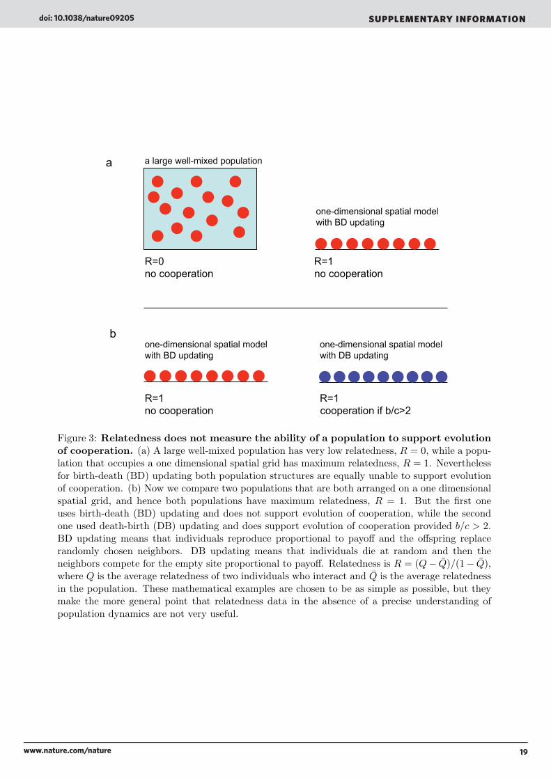
19www.nature.com/nature
SUPPLEMENTARY INFORMATIONdoi: 10.1038/nature09205
a large well-mixed population
one-dimensional spatial model
with BD updating
R=0 R=1
no cooperation no cooperation
R=1 R=1
no cooperation cooperation if b/c>2
one-dimensional spatial model
with BD updating
one-dimensional spatial model
with DB updating
a
b
Figure 3: Relatedness does not measure the ability of a population to support evolutionof cooperation. (a) A large well-mixed population has very low relatedness, R = 0, while a popu-lation that occupies a one dimensional spatial grid has maximum relatedness, R = 1. Neverthelessfor birth-death (BD) updating both population structures are equally unable to support evolutionof cooperation. (b) Now we compare two populations that are both arranged on a one dimensionalspatial grid, and hence both populations have maximum relatedness, R = 1. But the first oneuses birth-death (BD) updating and does not support evolution of cooperation, while the secondone used death-birth (DB) updating and does support evolution of cooperation provided b/c > 2.BD updating means that individuals reproduce proportional to payoff and the offspring replacerandomly chosen neighbors. DB updating means that individuals die at random and then theneighbors compete for the empty site proportional to payoff. Relatedness is R = (Q− Q)/(1− Q),where Q is the average relatedness of two individuals who interact and Q is the average relatednessin the population. These mathematical examples are chosen to be as simple as possible, but theymake the more general point that relatedness data in the absence of a precise understanding ofpopulation dynamics are not very useful.
19

20www.nature.com/nature
doi: 10.1038/nature09205 SUPPLEMENTARY INFORMATION
to show that there are clear limitations to inclusive fitness theory, if the Rj in (18) should stillresemble a meaningful relatedness. If one allows for a definition of Rj that is not even remotelyclose to a relatedness that could be measured, then we do not see what is gained from a kin selectionperspective. Pushing for such generalizations and extensions of inclusive fitness theory is not onlycumbersome and confusing but ultimately useless for two reasons: theoretically they bring nothingnew or even different from what is obtained with a simple, general, common sense result of theform (15) and empirically they have no value, because they do not use quantities that an empiricalbiologist could measure or call ‘relatedness’.
7.1 Non-vanishing selection
Inclusive fitness theory requires weak selection for two reasons. First of all, even for pairwise in-teractions, in order to remove synergistic effects, one needs games with equal gains from switching.The limit of weak selection as described in Section 2.1 ensures that the games have this prop-erty. However, even if theoreticians restrict themselves to games with equal gains from switching,in a stochastic process, they still need to take the limit of weak selection. This is because thestochasticity introduces effects of competition between individuals and these are not independentof the ‘helping’ events and thus they cannot simply be added or subtracted. To make these eventsindependent, one needs to be in the limit of weak selection.
Let us exemplify this second problem that arises for strong selection using the same one dimen-sional spatial model of Section 4. The birth rate of an individual is given by (27). In the limit ofweak selection, the effective payoff (score) of individual i is given by (28). Both approaches agreewith this in the limit of weak selection. However, a stronger selection variant has not yet beenproposed and so we will not explicitly write it here but simply say that the effective payoff (score)of individual i is a function of his own strategy as well as those of the neighbors fi(si−1, si, si+1).Let us consider DB updating. In this case the death rate is constant, d = 1/N . Then the averagenumber of offspring of individual i is given by (29). In this case, even in a given state, one cannotwrite additively the effects of an individual on everyone else in the population, simply becausewhen we take the derivative of wi with respect to sk, for some k, it is not necessarily independentof sj for j = 1, . . . , N . Let us exemplify this for simplicity, by taking the effects of an individual onhimself
∂wi
∂si=1N
∂fi
∂si(fi + fi−2)− ∂(fi+fi−2)
∂sifi
(fi + fi−2)2+
∂fi
∂si(fi + fi+2)− ∂(fi+fi+2)
∂sifi
(fi + fi+2)2
(40)
Clearly this quantity still depends (in a highly non-trivial way) on some si, si±1 and si±2. Thusthe effects of individuals on fitness are not independent (and certainly not linear) unless we are inthe limit of weak selection. Therefore, non-vanishing selection is not just harder to calculate butit fails to lend itself to an inclusive fitness interpretation. Not only does the final result look morecomplicated than bR > c, but the concept of identity by descent does not arise in the calculation.
Moreover, we point out that very interesting results have already been obtained for any intensityof selection using the common sense approach based on natural selection (Ohtsuki and Nowak 2006,Traulsen et al 2008, Antal et al 2009b).
20

21www.nature.com/nature
SUPPLEMENTARY INFORMATIONdoi: 10.1038/nature09205
7.2 Non-additive games
By a non-additive game we mean one where interactions are either synergistic or are not necessarilypairwise. In an ant colony it is hard to imagine that pairwise interactions are sufficient to specifyall fitness considerations. In fact, we expect that a synchronization of workers of different castes isnecessary for success. This scenario cannot be covered by inclusive fitness theory.
Attention to such synergistic games was drawn by Queller (1985) who looked at 2-player gamesthat do not have equal gains from switching. This is also discussed by Traulsen (2010). The ideawas however expanded to non-additive, multiple player games by van Veelen (2009) who referredto them as 3-person stag hunt games. Gokhale and Traulsen (2010) also analyze multiple playerone-shot games and point out the complex situations that can arise when pairwise interactions areinsufficient to describe the dynamics.
The idea behind van Veelen’s proposal is that it does not matter whether one or two of theplayers in a rock band rehearse – the band will sound lousy unless all three rehearse. A similarmetaphor can be imagined for ants. Consider the following game. Imagine there are groups of size3, all trying to accomplish a certain task, which can only be accomplished if all three individualscooperate. A member of a group has the option to either cooperate and thus incur a cost c ordefect. If all 3 individuals cooperate, they all incur the cost c but the task is accomplished andthey are all rewarded with a benefit b. Thus the payoff of a CCC group is (b − c, b − c, b − c). Ifneither cooperates, then they don’t pay any cost but they also don’t get any benefit. Then thepayoff of a DDD group is (0, 0, 0). However, and here comes the non-additivity of this game, ifonly one or two of the members cooperate and the others do not, the group does not accomplishthe goal and so no one gets a benefit. The payoff of a CCD group is (−c,−c, 0) and that of a CDDgroup is (−c, 0, 0).8
There are n such groups; hence the total population size is 3n. We label the individuals in agroup by 1, 2 and 3 and we specify individual 1 in group k by sk
1. There is no difference betweenthe 1, 2 or 3 roles. Thus, the effective payoff of individual 1 in triple k is given by
fk1 = 1 + δ(−csk
1 + bsk1s
k2s
k3) (41)
Therefore a benefit arises only if all three members of the group cooperate. Clearly in such a gameone cannot separate the effects of the action of the second player on the first from the effects of theaction of the first on himself.
To make this point even more clear, let us consider the following dynamics. At each updatestep, an individual is picked to change his strategy. The way he changes the strategy is by choosingsomeone proportional to payoff and imitating their strategy. Thus, the death rate is constantd = 1/3n and the birth rate of individual 1 in group k is bk
1 = fk1 /F where F =
k(f
k1 + fk
2 + fk3 ).
Then the average number of offspring of individual 1 in pair k is
wk1 = 1−
13n+
fk1
F(42)
which for weak selection becomes
wk1 = 1 +
δ
3n
− csk
1 + bsk1s
k2s
k3 −
13n
nj=1
− c(sj
1 + sj2 + sj
3) + 3bsj1s
j2s
j3
(43)
8As opposed to (b− 2c, b− 2c, 2b) and respectively (−2c, b, b) which would be the case in an additive game.
21

22www.nature.com/nature
doi: 10.1038/nature09205 SUPPLEMENTARY INFORMATION
Then, for example, the effect of individual 1 in group j = k on individual 1 in group k is
∂
∂δ
∂wk1
∂sj1
∼ c
9n2− b
3nsj2s
j3 (44)
This shows that the effect of individual sj1 on sk
1 is not independent of the action of other players; inparticular, it depends on the simultaneous action of the other two individuals from group j. In thiscase, one cannot separate the effects of the action of one actor on all recipients and hence the typeof inclusive fitness reasoning cannot be applied anymore. However, the general natural selectionargument can be successfully applied.
Here we want to point out that one could extend the inclusive fitness definition to also include‘relatedness’ of 3, 4, 5, ... individuals. However, the new definition will be far less intuitive;moreover, before applying such a definition one will need to know the actual model. Otherwise onecan never know whether they need to consider relatedness of 3 individuals or of 4 or of 5 and soon. Such an analysis will end up being the same as the game theoretic analysis.
7.3 Generic population structure
If the population structure is not fixed, but dynamical, varying from one state to the other, andis more complex than islands, then one cannot separate relatedness from the structure. Queller(1994) already pointed out that for limited dispersal models, the concept of relatedness has to belocal. Later Rousset and Billiard (2000) formalized this idea and showed that when the popula-tion is subdivided into islands (groups) one needs to compare the relatedness within a group tothe relatedness in the overall population. However, this approach does not completely solve theproblem. If individuals are always just on islands or on unweighted graphs (even if they are dynam-ical), it suffices to compare the relatedness of two people who interact to the average relatednessin the population. But if the population is on a dynamical, weighted graph, the situation becomesincreasingly more complicated. Then it is not so easy to pick two individuals who interact andcompare their relatedness to the average relatedness in the population, simply because two indi-viduals might interact with varying weights (some individuals might have weight 1, others weight1.5 and yet others weight 10). Since the structure is not fixed and these weights vary dynamicallyfrom one generation to the next, one cannot take a pair that has average weight either (because theaverage weight varies from one state to the next). Instead of needing to calculate quantities like
Pr(two individuals who interact are identical by descent) (45)
one now has to calculate quantities like
Pr(that they are identical in state)× (their average weight of interaction in that state)0 (46)
averaged over all states of the system, at neutrality. Since the average interaction weight of tworandom individuals varies with state, the above average cannot be broken down into the productof the probability that they are identical by descent, times the average weight of interaction.
Let us consider a specific example. Tarnita et al (2009a) propose a model based on set member-ships. We present here a somewhat simplified version of this model. Let us assume that individualshave exactly 2 tags 9. There are M possible tags. Two individuals interact depending how many
9If they could only have one tag each, this would be an island model as described by Antal et al (2009a) andTaylor and Grafen (2010)
22

23www.nature.com/nature
SUPPLEMENTARY INFORMATIONdoi: 10.1038/nature09205
tags they have in common. If they share 0, 1 or 2 tags, they have interaction weight 0, 1, or 2,respectively. At each time step, a randomly chosen individual updates his strategy and tags. Heimitates someone in the population proportional to payoff to obtain new tags and a new strategy.Therefore the population structure is dynamical. Depending on the state all individuals could havethe same two tags or they might be spread out over many different tags.
The interactions between individuals are dynamical, in the sense that they change from a stateto another. Individuals who might interact twice this week, might not interact at all next week.In each state we specify by vij ∈ {0, 1, 2} the interaction weight of i and j. For simplicity, letus assume that vij = vji. If vij = 0 then i and j do not interact. These interaction weights aredynamical in the sense that they change as a consequence of evolutionary updating. Then, in agiven state, the effective payoff (score, fecundity) of individual i is given by
fi = 1 + δ
j
vij(−csi + bsj) (47)
Since the death rate is at random, we have di = 1/N . The birth rate is proportional to effectivepayoff and all individuals compete for reproduction. Therefore, we have
bi =fi
F(48)
Here F is the total payoff in that given state. The average fitness of individual i is given by
wi = 1−1N+
fi
F(49)
For the limit of weak selection we obtain
wi = 1 +δ
N
j
vij(−csi + bsj)−1N
j
k
vjk(−csj + bsk)
= 1 +δ
N
si
− c+
c
N− b
N
j
vij +j =i
sj
bvij −
b− c
N
k
vjk
(50)
Clearly here the action of individual j on individual i depends on the dynamical structure. Theeffect of j on i is
∂wi
∂sj=
�− c+ c
N −bN
k vik if j = i
bvij − b−cN
k vjk if j = i
=(−c(N − 1)− b)vik if j = ibvij − (b− c)vjk if j = i
(51)
The second equality comes from replacing
l vkl = Nvkl; we do this by picking a random individualinstead of summing over all of them. Thus, the effect of the actor on himself is proportional tohow much he interacts with a random individual; the effect of a random individual on the actordepends on how much he interacts with the actor and on how much he interacts with someone atrandom.
Since this is a process with constant death, in the limit of weak selection but for any mutation,the condition for cooperators to be favored over defectors is given by (15). The individuals aresymmetric so instead of summing over all individuals as in (15), we can pick a random representative
23

24www.nature.com/nature
doi: 10.1038/nature09205 SUPPLEMENTARY INFORMATION
one, which we denote by •. Using (50) together with (51) we obtain the condition for cooperatorsto be favored over defectors:
(−c(N − 1)− b)v•ks•0 +j =•
(bv•j − (b− c)vjk)s•sj
0
> 0 (52)
This expression does not look like WIF > 0 anymore because what usually is identity by descentnow depends on the structure, containing quantities of the form v•js•sj0 which can no longer beinterpreted as local relatedness. This is because v•j changes from each state to the next and tocalculate such quantities, one needs to pick a random individual j in every state and multiply thenumber of tags the actor and j have in common with the probability that they are identical instate. This quantity is then averaged over all possible states.
In some sense, what a dynamical structure captures is the fact that I may be very related tomy sister but if I see her once a year now and maybe 100 times next year, this can make a hugedifference overall. Thus, for such dynamical structures genetic relatedness alone is not importantbut it somehow has to be weighted by the varying intensities of interaction.
8 Group selection is not kin selection
Group selection arises whenever there is competition not only between individuals but also betweengroups. Group selection is part of the more general concept of multi-level selection. There hasbeen a long and ongoing debate between scientists who work on group selection and kin selection(Wynne-Edwards 1962, Wilson 1975, Killingback et al 2006, Grafen 2007, Traulsen and Nowak2006, Lehmann et al 2007b, Wilson and Wilson 2007, Bijma and Wade 2008, Goodnight et al 2008,West et al 2008, West et al 2009, Wild et al 2009, van Veelen 2009, Traulsen 2010, Wade et al 2010)with the kin selection side claiming that group selection and kin selection are identical approaches.In the light of what we have shown here, we hope to settle this debate. Group selection models,if correctly formulated, can be useful approaches to studying evolution. Moreover, the claim thatgroup selection is kin selection is certainly wrong.
Group selection models can be formulated for any intensity of selection (Traulsen et al 2008).Since, when dealing with stochastic processes, inclusive fitness theory works only for the limitof weak selection, results for groups with non-vanishing selection cannot be replicated by such atheory. As we have pointed out weak selection results are interesting, but they do not offer acomplete picture of evolution. Hence, from the start, kin selection cannot possibly cover the sameground as group selection.10
If however we limit ourselves to weak selection, group selection can be interpreted in terms ofinclusive fitness calculations only if assumptions (i) and (ii) hold. But it is very easy and very naturalto formulate group selection models that violate the assumptions needed for an inclusive fitnesscalculation. Group selection models could contain non-additive games or dynamical populationstructures, where individuals interact with different intensities. Thus, even for weak selection,
10It is worth noting that for deterministic, replicator equation-type models, van Veelen (2009) shows that groupselection models and inclusive fitness models give the same prediction even for non-vanishing selection, as long as theinclusive fitness theory restricts itself to the non-generic case of games with equal gains from switching. However,such a result does not hold for stochastic models, where the inclusive fitness method requires weak selection notonly to obtain equal gains from switching, but also to make the interactions and competitions between individualsindependent and additive (Section 7.1).
24

25www.nature.com/nature
SUPPLEMENTARY INFORMATIONdoi: 10.1038/nature09205
group selection cannot in general be described by inclusive fitness calculations. The claim thatthey are identical, which has often been made (Lehmann et al 2007b, West et al 2008, Wild et al2009), is wrong.
9 Summary
We emphasize the following points:
• Inclusive fitness is just another method of accounting. The fact that an inclusivefitness calculation works for a particular model does not necessarily imply that ‘kin selectionis at work’. Inclusive fitness theoreticians have been inconsistent about this point. Originally,they suggested that it is just another method of calculation and stressed that Hamilton’s1964 paper is ‘devoted to proving that the alternative accounting procedure that underliesinclusive fitness gives the same answer as the standard and logically prior procedure’ (Grafen1984). We agree with this perspective but add that, as we have proved in this paper, theinclusive fitness method cannot be used as widely as the logically prior and more generalprocedure based on natural selection.
Of course, theoreticians are free to use any method of calculation as long as they employit correctly and do not make unjustified statements claiming a ‘general principle’ for theevolution of cooperation (Lehman et al 2007a,b, Wild et al 2009, West et al 2008, Gardner2009, West and Gardner 2010). A method of calculation which is arguably more cumbersomeand confusing is not a general principle, much like the ptolemaic epicycles in the solar systemwere not a general principle either and became superfluous under Newtonian mechanics.
We have a similar situation in this debate. The epicycles of inclusive fitness calculations arenot needed, given that we can formulate precise descriptions of how natural selection acts instructured populations.
• Inclusive fitness is not nearly as general as the game theoretic approach based onnatural selection. As we have pointed out here, the concept of inclusive fitness only leadsto correct results if a number of constraining assumptions hold. These are the limit of weakselection together with assumptions (i) additive games and (ii) very simplistic populationstructures.
• Inclusive fitness is often wrongly defined. Inclusive fitness is NOT the sum of anindividual’s offspring plus the offspring of the relatives. It only includes an individual’s ownoffspring that come as a result of his own actions, but not as a result of the help receivedfrom others. Thus my inclusive fitness is:
(my offspring resulting from my own actions but NOT from the help I receive from others)+R × (my relatives’ offspring resulting from my helping them)
This definition is somewhat artificial and leads to significant confusion in practice. Grafen(1984) warned empiricists and theoreticians against incorrect usage of the term and advisedempiricists against using inclusive fitness altogether. Instead, they are told to use Hamilton’srule. This suggestion, however, brings us to another problem.
25

26www.nature.com/nature
doi: 10.1038/nature09205 SUPPLEMENTARY INFORMATION
• Hamilton’s rule almost never holds. For the limit of weak selection, we often find thatcooperation is favored over defection provided ‘something’ is greater than the cost to benefitratio. This result is not the consequence of inclusive fitness theory, but arises because of thelinearity introduced by weak selection (Wild and Traulsen 2007, Tarnita et al 2009b). Aswe have shown here, however, ‘something’ is almost never ‘relatedness’, even if we are in aspecial situation where inclusive fitness can be formulated.
The validity of Hamilton’s rule is also challenged by economists. Alger and Weibull (2009)show that the evolutionarily stable degree of altruism (threshold cost-to-benefit ratio) is lowerthan the degree of relationship; moreover, it strongly depends on the environment, which isnot something inclusive fitness theoreticians consider. The analysis of Alger and Weibull(2009) suggests a reason why weaker family ties may have developed in harsher climates, andhow this may have induced stronger economic growth, according to Macfarlane (1978, 1992).
• Relatedness measurements without a model of population dynamics are incon-clusive. While relatedness measurements in the field can provide useful information aboutpopulation structure, they do not provide immediate information for the evolution of coop-eration. Relatedness measurements always must be interpreted in the context of a modelof evolutionary dynamics. Otherwise they can lead to meaningless conclusions. Relatednessmeasurements alone are not a test for inclusive fitness theory.
• Inadequacy of inclusive fitness. Let us consider a situation where one individual pays acost to benefit another individual. If the two individuals are related, then there is a probabilitythat they might both carry the same gene that affects altruistic behavior, and hence that genecould have a fitness advantage. We have shown that inclusive fitness theory cannot decidein general if an allele that makes you help a relative is favored by natural selection or not.Instead we need a calculation that is based on a precise description of population structureand dynamics.
26

27www.nature.com/nature
SUPPLEMENTARY INFORMATIONdoi: 10.1038/nature09205
Part B – Empirical tests reexamined
Faith in the central role of kinship in social evolution, defined in one manner or other, has led tothe reversal of the usual order in which biological research is conducted. The proven best way inevolutionary biology is to define a problem arising during empirical research, then select or devisethe theory that is needed to solve it. Almost all research in inclusive fitness theory has been theopposite: hypothesize the key roles of kinship and kin selection, then look for evidence to test thathypothesis.
The most basic flaw in this approach is failure to consider multiple competing hypotheses.Often the measurement of pedigree kinship becomes a surrogate for an in-depth study of naturalhistory of the species. When the data do not fit, elaborations of inclusive-fitness theory can beconstructed that make them fit. The results of the elaborations are a ptolemaic theory, constructedof epicycles to keep relatedness at the center of evolving social systems. With enough of epicycles,they can even be made to fit the data, but, as in the geocentric theory of the cosmos, at the cost ofusing the wrong starting assumption. This misstep in logic is known as ‘Affirming the Consequent.When biological details of particular cases are examined before inclusive fitness theory is applied,alternative explanations from standard natural selection theory come quickly to attention. Wehave examined an array of the most meticulously analyzed cases presented by various authorsas evidence for the success of kin selection theory. Without exception it has been easy to findweaknesses in each case, suggesting that analyses of empirical observations based on kin selectiontheory alone are typically inconclusive. We know of no case that presents compelling evidencefor the explanatory adequacy of kin selection and inclusive fitness theory. Three representativeexamples of the inadequacy are the following.
First, Hughes et al (2008) argue that the origin of eusociality is driven by close kinship, becausein basal clades of eusocial ants, bees and wasps, queens mate only with a single male and thereforeproduce a colony of closely related individuals. The authors present their data as correlativeevidence of kin selection promoting the evolution of eusociality. However, comparable data werenot provided for solitary clades, including sister clades of the eusocial examples, hence there wereno controls for the retrodiction of kin selection. In fact, it is logical to suppose that such queens alsomate with one male only, and for a reason unrelated to kin selection: prolonged mating excursionsincrease the risk to young females from predators. Thus even at best it is not proved that singlemating and the resulting close relatedness of offspring is an important factor in promoting theevolution of eusociality. Of equal importance, Hughes et al (2008) point to the origin of multiple-male matings practiced by queens of many clades with advanced colonial organization. This, theyconclude, indicates the relaxation of kin selection in later stages of evolution. But they overlook themuch simpler explanation that in species with exceptionally large worker populations, queens needmultiple matings in order to store enough sperm. Further, and oddly, many studies have foundthat, as a rule, members of social insect colonies cannot recognize their own degree of pedigreerelatedness to their nestmates (Holldobler & Wilson 2009, Ratnieks et al 2006). For ants at least,membership in a particular colony is determined by the overall colony odor learned by each adultduring the first several days following her emergence from the pupa as an adult. For this reasonit is possible to experimentally produce colonies whose members differ from one another radically,even belonging to different species. Such is the basis of slavery practiced by some parasitic antspecies (Holldobler & Wilson 2009, Ratnieks et al 2006). Is such learning just a proxy for stayingclose to genetic kin? Perhaps, but a more likely selection force is communal fidelity and defense ofthe nest, as we have documented in the main text.
27

28www.nature.com/nature
doi: 10.1038/nature09205 SUPPLEMENTARY INFORMATION
In another, very different setting, a meticulous experimental analysis using the periodicallysubsocial eresid spider Stegodyphus lineatus, has demonstrated that groups of sibling spiderlingsextract more nutrients from communal prey than do spiderlings of artificially mixed parentage(Schneider & Bilde 2008). Because injecting digestive enzymes is costly, the authors suggest thatindividuals withhold their enzymes to avoid exploitation by strangers. The authors accept the kinselection hypothesis. The problem is that in their natural habitat these spiderlings (necessarilycoming from the same mother) never find themselves in mixed groups. Hence, we would notexpect any specific adaptation to deal with such a situation. A much simpler explanation forthe observed reduction in communal intake is given by discordance among unrelated individuals(meaning they are not working together efficiently). Such discordance is a general principle, whichis often overlooked by kin selection based explanations. Genetically diverse groups (especially thosethat are generated artificially in an experimental situation) are prone to be less harmonious, becausethe individuals are not necessarily adapted to work with each other.
A third process that can lead to seeming kin-based altruism but is more simply and realisticallyexplained otherwise is the expectation of inheritance. In a small percentage of bird and mammalspecies, offspring remain at the nest of their birth and assist their parents in rearing additionalbroods. They thereby delay reproduction on their own while increasing reproduction of theirparents. In one interpretation, Griffin and West (2003) attribute the phenomenon to kin selection,and bolster their argument by demonstrating a positive correlation across species between closenessof kinship and the amount of help provided to parents by the stay-at-homes. However, morethorough, previously published studies, covering life history data in a wide range of species, hadalready arrived at a simpler explanation of why, under certain conditions unrelated to kin selection,the persistence of adult young at the natal nest is favored. The conditions include unusual scarcityeither of nest site or territory or both, generally low adult mortality, and relatively unchangingconditions in a stable environment. After prolonged residence, the helpers inherit the nest orterritory upon the death of the parents (Hatchwell & Komdeur 2000). The positive correlationacross species between kinship and helping reported by Griffin and West, is based on a few widelyscattered data points, but if upheld might well be explained by the common practice of the floaterstrategy in some species (Hatchwell & Komdeur 2000), in which individuals move about nests andspread the amount of help given.
28

29www.nature.com/nature
SUPPLEMENTARY INFORMATIONdoi: 10.1038/nature09205
Part C – A mathematical model for the origin of eusociality
We consider a species of solitary insects (wasps or others) where fertilized females build nests andraise their offspring by progressive provisioning. Once the larvae hatch, the offspring leave thenest. We call this the solitary life cycle. As outlined in the main text, we then assume that amutant arises, where the offspring do not necessarily leave the nest. Those young that stay at thenest engage in the task of helping their mother to raise her subsequent offspring. Hence, they donot reproduce themselves, but sacrifice their reproductive potential to help another individual toreproduce. We call this the eusocial life cycle. We study the conditions for natural selection tofavor the eusocial strategy over the solitary one.
At first we design a model with asexual reproduction in order to understand the essence ofthe problem. Subsequently we develop a model with sexual reproduction, taking into account thehaplodiploid genetics of Hymenoptera. In both cases, we see that very different mathematicalstructures arise from those that were considered by kin selection theorists over the last decades.The kin selectionist’s framing of the problem in terms of cost and benefit of the worker is notnatural, and an inclusive fitness type calculation is not necessary.
Our model differs from previous approaches. Wade (1978) performs an interesting populationgenetic analysis of a situation where the broods of several females develop in close proximity andcooperate with each other to some extent. Craig (1979, 1983) explores parental manipulationand subfertility, which are potential mechanisms for the evolution of eusociality (Alexander 1974,Michener & Brothers 1974, West-Eberhard 1975, Charnov 1978) sometimes subsumed under kinselection (Bourke & Franks 1995). Gadagkar (1990) argues that eusociality could have arisenvia several different mechanisms and what is important is not only its emergence but also itsmaintenance. Lehmann et al (2008) study a model where sterile workers migrate between coloniesoffering their help to different queens, but this is an unlikely biological scenario for the evolutionof eusociality.
The theory that we develop here represents the simplest possible and most direct approach toevaluate how natural selection acts on alleles prescribing social behavior. The target of selection isneither the phenotypic trait of the queen in particular, nor that of the colony, but the collectivityof traits that modify social behavior at both these levels. The traits can be evaluated separatelyand together.
10 Asexual reproduction
10.1 A simple linear model
We consider deterministic evolutionary dynamics described by ordinary differential equations. Letx0 denote the abundance of solitary females. They reproduce at rate b0 and die at rate d0. Let xi
denote the abundance of eusocial nests (colonies) of size i. Here i = 1, 2, ... represents the number ofindividuals working at the colony including the queen. Thus, x1 denotes nests with single eusocialqueens, while x2 denotes nests where a queen has one worker, and so on.
A eusocial queen in a nest of size i has reproductive rate bi and death rate di. We assume thatthe presence of workers allows the queen to stay with the nest, which might increase her rate ofoviposition and reduce her death rate. There is less risk of predation both for the queen and for theeggs, which can be guarded by the queen and other workers. The queen in particular can redirect
29

30www.nature.com/nature
doi: 10.1038/nature09205 SUPPLEMENTARY INFORMATION
her resources from foraging to laying eggs and protecting them. The offspring of the eusocial queenstay with the nest with probability q and leave the nest with probability 1− q. In the latter casethey start their own nest.
Evolutionary dynamics of the two strategies are described by the following system of lineardifferential equations
x0 = (b0 − d0)x0
x1 =∞i=1
bi(1− q)xi − b1qx1 − d1x1
xi = bi−1qxi−1 − biqxi − dixi i = 2, 3, ...
(53)
The strategy with the faster growth rate wins eventually. The exponential growth rate of thesolitary strategy is b0− d0, while that of the eusocial strategy is given by the largest eigenvalue, λ,of the matrix
M =
b1(1− q)− (b1q + d1) b2(1− q) b3(1− q) b4(1− q) . . .b1q −(b2q + d2) 0 0 . . .0 b2q −(b3q + d3) 0 . . .0 0 b3q −(b4q + d4) . . ....
......
.... . .
(54)
If λ > b0 − d0 then eusociality wins over solitary. If λ < b0 − d0 then solitary wins. The caseλ = b0 − d0 is ungeneric. Matrix, M , can be seen as a ‘mutation-selection matrix’ as it occurs forexample in quasispecies theory (Eigen & Schuster 1977). Formally speaking the growth of colonies,described by the parameter q, denotes a ‘mutation term’ between colonies of different size. Thelargest eigenvalue of M is the fitness of the ‘quasispecies’.
Whether or not eusociality is selected depends on how the demographic parameters of the queenchange with colony size. One possibility is to consider a simple step function with a critical colonysize, m. For small colonies, i < m, the key parameters of the eusocial queen are the same as thoseof solitary females: bi = b0 and di = d0. For large colonies, i ≥ m, the eusocial queen has anincreased fecundity and a reduced death rate: bi = b > b0 and di = d < d0.
A necessary condition for the evolution of eusociality is
b− kmd > km(b0 − d0) (55)
The number km depends on the critical colony size, m, where the advantages of eusociality arise. Itturns out that km grows exponentially with m: we have k2 = 2, k3 = 9, k4 = 28, k5 ≈ 76, k6 ≈ 196and so on. It is essential that already small colonies increase the reproductive rate, b, of the queen.Otherwise it is very hard for eusociality to be selected. Despite its obvious and intuitive advantagesit is in fact not easy to evolve eusociality.
Condition (55) is necessary but not sufficient. If (55) holds then there exist values of q thatallow eusociality to win. There is a lower bound, qmin, and an upper bound, qmax. Eusocialitywins if qmin < q < qmax. For m = 2 we find qmin = 0 and qmax = 1− 2(b0 − d0 + d)/b. For m ≥ 3we have 0 < qmin < qmax < 1. Depending on the value of b we observe that eusociality sometimeswins only for a narrow range of q values.
30

31www.nature.com/nature
SUPPLEMENTARY INFORMATIONdoi: 10.1038/nature09205
10.2 Adding density limitation
We can add density limitation by multiplying each birth term with a factor φ that representsdeclining food resources as the total population size increases. A natural possibility is φ = 1/(1 +ηX) where η is a parameter that scales the size of the system and X = x0 +
i ixi is the total
population size. The system with density limitation can be written as
x0 = (b0φ− d0)x0
x1 =∞i=1
biφ(1− q)xi − b1φqx1 − d1x1
xi = bi−1φqxi−1 − biφqxi − dixi i = 2, 3, ...
(56)
The mathematical analysis is very similar to that in the previous section. There is no coexistencebetween the two strategies. One strategy will exclude the other. We must find the largest eigenvalue,λ, of the matrix
M =
b1(1− 2q)/d1 b2(1− q)/d1 b3(1− q)/d1 b4(1− q)/d1 . . .b1q/d2 −b2q/d2 0 0 . . .0 b2q/d3 −b3q/d3 0 . . .0 0 b3q/d4 −b4q/d4 . . ....
......
.... . .
(57)
As before, eusociality is selected if λ > b0 − d0. Let us consider the same step function as before,where the advantages of eusociality arise if the colony size is at least m. We find a similar necessarycondition for the evolution of eusociality, b/d > km(b0/d0). The numbers km are the same as before.The expressions for qmin and qmax are also slightly different. For example, for m = 2 we haveqmin = 0 and qmax = 1 − 2b0d/(bd0). Again, for m ≥ 3 we find that eusociality wins only for arestricted range of q values, 0 < qmin < q < qmax < 1.
10.3 Adding worker mortality
In the previous models the mortality of workers was somehow folded into the reproduction rate ofthe queen, but here we explicitly assume that workers die at rate α. We obtain
x0 = (b0φ− d0)x0
x1 =∞i=1
biφ(1− q)xi − b1φqx1 − d1x1 + αx2
xi = bi−1φqxi−1 − biφqxi − dixi − α(i− 1)xi + αixi+1 i = 2, 3, ...
(58)
As before we use φ = 1/(x0+η
i ixi). Again there is no coexistence between the solitary strategyand the eusocial one. There are two equilibria. At the solitary equilibrium x0 is positive and allxi (with i = 1, 2, ...) are zero. At the eusocial equilibrium x0 is zero and all xi (with i = 1, 2, ...)are positive. One equilibrium is stable and the other one unstable with respect to invasion by theopposite strategy. The stable equilibrium is the one that establishes the larger total populationsize. This criterium specifies whether or not eusociality is favored by natural selection.
31

32www.nature.com/nature
doi: 10.1038/nature09205 SUPPLEMENTARY INFORMATION
Figure 4 shows how the winning strategy changes as a function of the parameter q, which denotesthe probability that a eusocial offspring stays with the nest. For small values, 0 < q < 0.36, and forlarge values, 0.9 < q < 1, the solitary strategy wins. For the intermediate region, 0.36 < q < 0.9,the eusocial strategy wins. In this numerical example the solitary female has reproductive rateb0 = 0.5, which means she lays one (surviving) egg every other day. Her death rate is d0 = 0.1,which implies an average life time of 10 days. The solitary female has to lay eggs and then go outto search for food, which exposes both the eggs and herself to risk from predation. The eusocialqueen has the same parameters unless the colony reaches a critical size, here m = 3. Subsequentlyher reproductive rate increases 8-fold and her death rate decreases 10-fold. Thus for all i ≥ mwe assume bi = 4 and di = 0.01. She has less risk of predation and can devote her resources tolaying eggs and protecting them. We assume that the workers in the eusocial colony have the samedeath rate as solitary individuals, α = 0.1. Finally we assume, if the queen dies then the colonydisappears.
Note that intermediate q values are needed for eusociality to evolve. The intuitive explanationis as follows. For low q there is only a small probability that the colony reaches the critical size,m, where the advantage of eusociality begins. On the other hand, if the value of q is too large thenthe colonies produce too few new queens. Of course, the disadvantage of eusociality is that some ofthe offspring (workers) do not reproduce; they are subject to worker mortality and they die whenthe queen dies. Therefore, intermediate values of q allow the evolution of eusociality.
The situation that we observe here is not a standard cooperative dilemma (Hauert et al 2006,Nowak 2006, Nowak et al 2010). An offspring that stays with the nest could be seen as a ‘coopera-tor’, an offspring that leaves could be seen as a ‘defector’, but the optimum strategy of eusocialityhas an intermediate level of cooperators and defectors. ‘Defectors’ (new queens) are needed for thereproduction of eusociality.
11 Sexual reproduction and haplodiploid genetics
We now develop a model that takes into account sexual reproduction and the haplodiploid geneticsof Hymenoptera. We study competition between two alleles: the wildtype allele, A, and the mutantallele a. The mutant allele disrupts the dispersal behavior of females as described in the main text.It can either act in a dominant or recessive way. Denote by q1, q2, q3 the probabilities that AA, Aaand aa females stay with the nest. If the mutation is dominant, we have q1 = 0 and q2 = q3 > 0.If the mutation is recessive, we have q1 = q2 = 0 and q3 > 0.
There are three types of females, AA, Aa, aa, and two types of males, A and a. There are sixtypes of fertilized females (queens), which we denote by AA-A, AA-a, Aa-A, Aa-a, aa-A and aa-a.The first two letters specify her own genotype, while the third letter specifies the genotype of thesperm she has received and stored. For example, AA-a means that an AA female has mated withan a male. Such an AA-a queen produces Aa females and A males. In contrast an Aa-A queenproduces equal proportions of AA and Aa females and equal proportions of A and a males.
Let us introduce the following notation: XAA-A,i denotes the abundance of colonies of size ifounded by an AA-A queen; similarly XAA-a,i denotes the abundance of colonies of size i foundedby an AA-a queen, and so on. The queen in a colony of size i has birth rate bi and death rate di.The mortality of workers is given by α. The abundances of virgin queens (females who have leftthe nest and try to mate) is given by xAA, xAa and xaa. The abundance of males is given by yA
and ya. The parameter β characterizes the rate of successful mating.
32

33www.nature.com/nature
SUPPLEMENTARY INFORMATIONdoi: 10.1038/nature09205
Figure 4: Eusociality evolves for intermediate values of q, which is the probability that offspringstay with the nest. Furthermore, the eusocial queen must have a dramatically increased rate ofoviposition, b. The figure shows equilibrium values of the model given by (58). Parameter valuesare b0 = 0.5, d0 = 0.1, m = 3, b = 4, d = 0.01 and α = 0.1. Hence, eusocial queens that have atleast two workers have an 8-fold increased rate of laying eggs and a 10-fold reduced death rate. Theupper panel shows the number of individuals, where red indicates solitary, x0, and blue eusocial,
i ixi. The lower panel shows the total number of colonies with at least one worker,
i xi, wherei = 2, 3, .... Note that eusociality is selected if approximately 0.36 < q < 0.9 .
33

34www.nature.com/nature
doi: 10.1038/nature09205 SUPPLEMENTARY INFORMATION
We have the following system (the index i runs from 2, ..∞):
XAA-A,1 = βxAAyA − b1q1XAA-A,1 − d1XAA-A,1 + αXAA-A,2
XAA-A,i = q1(bi−1XAA-A,i−1 − biXAA-A,i)− diXAA-A,i − α(i− 1)XAA-A,i + αiXAA-A,i+1
XAA-a,1 = βxAAya − b1q2XAA-a,1 − d1XAA-a,1 + αXAA-a,2
XAA-a,i = q2(bi−1XAA-a,i−1 − biXAA-a,i)− diXAA-a,i − α(i− 1)XAA-a,i + αiXAA-a,i+1
XAa-A,1 = βxAayA − b1q1 + q2
2XAa-A,1 − d1XAa-A,1 + αXAa-A,2
XAa-A,i =q1 + q2
2(bi−1XAa-A,i−1 − biXAa-A,i)− diXAa-A,i − α(i− 1)XAa-A,i + αiXAa-A,i+1
XAa-a,1 = βxAaya − b1q2 + q3
2XAa-a,1 − d1XAa-a,1 + αXAa-a,2
XAa-a,i =q2 + q3
2(bi−1XAa-a,i−1 − biXAa-a,i)− diXAa-a,i − α(i− 1)XAa-a,i + αiXAa-a,i+1
Xaa-A,1 = βxaayA − b1q2Xaa-A,1 − d1Xaa-A,1 + αXaa-A,2
Xaa-A,i = q2(bi−1Xaa-A,i−1 − biXaa-A,i)− diXaa-A,i − α(i− 1)Xaa-A,i + αiXaa-A,i+1
Xaa-a,1 = βxaaya − b1q3Xaa-a,1 − d1Xaa-a,1 + αXaa-a,2
Xaa-a,i = q3(bi−1Xaa-a,i−1 − biXaa-a,i)− diXaa-a,i − α(i− 1)Xaa-a,i + αiXaa-a,i+1
(59)
For virgin queens we have:
xAA = (1− q1)
i
bi(XAA-A,i +12XAa-A,i)− xAA(g + βy)
xAa = (1− q2)
i
bi(XAA-a,i +12XAa-A,i +
12XAa-a,i +Xaa-A,i)− xAa(g + βy)
xaa = (1− q3)
i
bi(12XAa-a,i +Xaa-a,i)− xaa(g + βy)
(60)
For males we have
yA =
i
bi(XAA-A,i +XAA-a,i +12XAa-A,i +
12XAa-a,i)− hyA
ya =
i
bi(12XAa-A,i +
12XAa-a,i +Xaa-A,i +Xaa-a,i)− hya
(61)
Here g and h denote respectively the death rates of virgin queens and males. Note that virginqueens become fertilized queens after mating. Hence, the term βy is added to their death rate,where y = yA + ya is the total abundance of males. We assume that males do not die because ofthe mating, but they have a very short life span. Hence it is unlikely that a male mates twice.Finally, we assume that males and females are produced at the same rate, an assumption whichcould easily be modified by introducing an additional parameter.
For computer simulations we add density limitation by multiplying each birth term with a factorφ = 1/(1 + ηX) where η is a constant and X is the total population size.
Figure 5 shows the equilibrium structure of the sexual model assuming that the eusocial allele,a, is recessive. This means that aa females stay with the nest with probability q, while AA and
34

35www.nature.com/nature
SUPPLEMENTARY INFORMATIONdoi: 10.1038/nature09205
Aa females always leave the nest. Therefore, ‘full-sized’ colonies are formed by aa-a queens and‘half-sized’ colonies are formed by Aa-a queens. All daughters of aa-a queens are aa and stay withthe nest with probability q. Half of the daughters of Aa-a queens are aa, who stay with the nestwith probability q, while the other half are Aa who leave the nest. All other fertilized females aresolitary, because all of their offspring leave the nest. We assume that all males leave the nest.
We use the same parameter values as for the asexual simulation. The birth rate of a solitaryqueen is b0 = 0.5 and her death rate is d0 = 0.1. The benefits of eusociality emerge once the colonyreaches a critical size of m = 3. For all colony sizes, i ≥ m, the birth rate of the queen is b = 4and her death rate is d = 0.01. We make the following observation. As long as q < 0.7 the solitaryallele is selected: all females are AA and all males are A. At q ≈ 0.7 there is a sudden reversal.For 0.7 < q < 0.88 the eusocial allele outcompetes the solitary one: all females are aa and allmales are a. But for q > 0.88 we find that heterozygote females, Aa, become abundant; now manycolonies are now founded by Aa females that have mated with a males. Figure 5 shows the stableequilibrium that is reached from an initial state where the eusocial allele, a, is rare. This initialcondition is relevant, if we want to study the origin of eusociality in a world of solitary insects.
Figure 6 uses the same parameter values as Figure 5, but this time we show the stable equilibriumthat is reached when starting from a state where the solitary allele is rare. This initial conditionis relevant, if we want to study the evolutionary stability of eusociality. This time we find that thesolitary allele, A, wins if 0 < q < 0.26, while the eusocial allele, a, wins if 0.26 < q < 0.88. For0.88 < q < 1 there is coexistence of the two alleles.
We have the following situation. There are three critical thresholds of q. In our numericalexample they are qc1 ≈ 0.26, qc2 ≈ 0.7, qc3 ≈ 0.88. If 0 < q < qc1 the solitary allele wins. Ifqc1 < q < qc2 then we observe bi-stability; either the solitary or the eusocial allele wins dependingon initial condition. This means each homogeneous population is stable against invasion by theother allele. If qc2 < q < qc3 then the eusocial allele wins. If qc3 < q < 1 then there is coexistencebetween the two alleles.
12 Summary
We have proposed a model for the origin of eusociality. The basic idea is that a mutation preventssome daughters from leaving the nest. We study if this mutant allele is favored by natural selection.The fundamental consideration is the following: how are the key demographic parameters of theeusocial queen (her fecundity and her death rate) affected by the presence of workers. We findthat eusociality is selected if the fecundity of the queen increases dramatically while colony sizeis still small. This means that a eusocial queen that is supported by a few workers must alreadyhave a significantly increased rate of oviposition, must be more successful at guarding the larvae,and having them fed until they hatch. The evolution of eusociality is also favored if the queen hasa reduced death rate in the presence of workers. Both effects can arise naturally given that theeusocial queen stays at the nest, thereby reducing her risk of predation and devoting her resourcesto laying eggs and guarding them. Interestingly, we find that a reduced death rate alone is notsufficient for the evolution of eusociality. An increased birth rate is necessary.
A key observation of our model is that it is difficult to evolve eusociality, because we needvery favorable parameters. In our numerical examples we assumed that a eusocial queen withtwo workers has an 8-fold increased birth rate and a 10-fold reduced death rate. For the sameparameter choices, for example, a 7-fold increased birth rate would not have allowed the evolution
35

36www.nature.com/nature
doi: 10.1038/nature09205 SUPPLEMENTARY INFORMATION
Figure 5: Emergence of eusociality in a model with haplodiploid genetics. We study the competitionbetween a wildtype allele, A, and a recessive mutant allele, a. There are three types of females:AA (red), Aa (green) and aa (blue); aa females stay with the nest with probability q. There aretwo types of males: A (red) and a (blue). We simulate the system given by (59) - (61) showingthe equilibrium that is reached from an initial condition where the solitary allele, A, dominatesthe population. For 0.7 < q < 0.88 the eusocial allele replaces the solitary one. For 0.88 < q < 1there is coexistence. Parameter values: b0 = 0.5, m = 3, b = 4, β = 0.1, η = 0.01; mortality rates:d0 = α = g = h = 0.1 and d = 0.01.
36
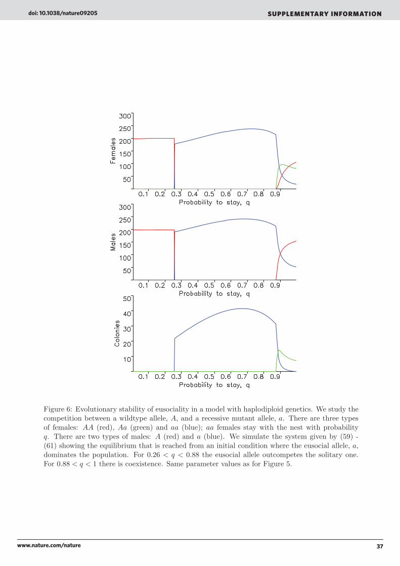
37www.nature.com/nature
SUPPLEMENTARY INFORMATIONdoi: 10.1038/nature09205
Figure 6: Evolutionary stability of eusociality in a model with haplodiploid genetics. We study thecompetition between a wildtype allele, A, and a recessive mutant allele, a. There are three typesof females: AA (red), Aa (green) and aa (blue); aa females stay with the nest with probabilityq. There are two types of males: A (red) and a (blue). We simulate the system given by (59) -(61) showing the equilibrium that is reached from an initial condition where the eusocial allele, a,dominates the population. For 0.26 < q < 0.88 the eusocial allele outcompetes the solitary one.For 0.88 < q < 1 there is coexistence. Same parameter values as for Figure 5.
37

38www.nature.com/nature
doi: 10.1038/nature09205 SUPPLEMENTARY INFORMATION
of eusociality. This observation is interesting: despite the obvious and intuitive advantages ofeusociality, it is very hard for a solitary species to achieve it.
Whether or not the circumstances can be that favorable for eusociality depends on the ecologicalenvironment of the pre-eusocial species under consideration. As outlined in the main text, a keyfactor is whether it is possible to establish and defend a valuable nest site that is close enough toa rich food source.
Another interesting aspect of our haplodiploid model is the occurrence of bistability. It iseasier to maintain eusociality than to evolve it. For a wide parameter region the eusocial allelecannot invade the solitary allele, and vice versa the solitary allele cannot invade the eusocial one(compare Figs 4 and 5). This property of the model explains in part why, even though eusocialityis ecologically dominant, the condition has evolved rarely in the history of life.
Our model leads to a number of radical new suggestions for research on eusociality.(i) Contrary to the prevailing dogma of inclusive fitness theory, it is not useful to view eusociality
as an evolutionary game between workers and queens. Inclusive fitness theory claims to be a gene-centered approach, but instead it is ‘worker-centered’. It puts the worker into the center of theanalysis and asks the (puzzling) question: why does a worker sacrifice her reproductive potentialto help raise the offspring of the queen? But if we put the gene into the center of the analysis (aswe have done) then this question of altruism does not even appear. A standard selection equationdetermines if the eusocial allele wins over the solitary one. There is no payoff matrix, there isno evolutionary game on the decisive level of competition. By formulating a model of populationgenetics in the context of family structure, we find that there is no need for the inclusive fitnessdetour.
(ii) The queen and her workers are not engaged in a standard cooperative dilemma. The reasonis that the workers are not independent agents. Their properties are determined by the alleles thatare present in the queen (both in her own genome and in that of the sperm she has stored). Theworkers can be seen as ‘robots’ that are built by the queen. They are part of the queen’s strategyfor reproduction.
(iii) It is not useful to describe a female who stays with the colony as ‘altruistic’ and a femalewho leaves as ‘selfish’. Both types of females are needed for the reproduction of the colony.
(iv) Our model does not use standard multilevel selection. There is only one level of selection,the hymenopteran colony, which is treated as an extension of the queen, whose genes are the unitsof selection. Selection operates between queens and solitary females or between different queens.
(v) Relatedness does not drive the evolution of eusociality. We can use our model to studythe fate of eusocial alleles that arise in thousands of different presocial species with haplodiploidgenetics and progressive provisioning. In some of those species eusociality might evolve, while inothers it does not. Whether or not eusociality evolves depends on the demographic parameters ofthe queen (as discussed above), but not on relatedness. The relatedness parameters would be thesame for all species under consideration.
(vi) Once eusociality has evolved, colonies consist of related individuals, because daughters staywith their mother to produce further offspring. Thus, relatedness is a consequence of eusociality,but not a cause.
(vii) Our model has clear implications for productive empirical research. The crucial mea-surement that needs to be performed is the effect of the size of the colony on the demographicparameters of the queen, such as her oviposition rate and average longevity. The animals mostlikely to yield significant data are the primitively eusocial bees and wasps, of which there are a
38

39www.nature.com/nature
SUPPLEMENTARY INFORMATIONdoi: 10.1038/nature09205
large number of species representing finely divided grades of evolution – including those that havereverted from eusociality to the solitary condition. There is moreover a need to identify the geneticcoding of the solitary-eusocial transition, as well as to identify the phenotypic flexibility of thegenes involved and the environmental pressures that drive selection.
Finally, we propose that kin selection among social insects is an apparent phenomenon whicharises only when you put the worker into the center of evolutionary analysis. Kin selectionistshave argued that a worker who behaves altruistically by raising the offspring of another individual,requires an explanation other than natural selection, and this other explanation is kin selection.We argue, however, that there exists a more convenient coordinate system. If the eusocial gene isin the center of the evolutionary analysis, then a standard natural selection equation determineswhether or not eusociality wins. There is no paradoxical altruism that needs to be explained. Theepicycles of kin selection and inclusive fitness disappear.
13 Acknowledgements
We thank Tibor Antal and Hisashi Ohtsuki for many discussions regarding the general frameworkpresented in Part A of the online material. We thank Matthijs van Veelen for valuable insightsinto additive games. We thank Radu Berinde, David Haig, David Hughes, Daniel Kronauer, ErezLieberman, David Rand and Arne Traulsen for helpful discussions. We thank Lydia Liu for helpwith the preparation of the manuscript.
References
Alger I and Weibull JW (2009). Kinship, incentives and evolution” (2009). forthcoming AmericanEconomic ReviewAlexander R D (1974). The evolution of social behaviour. Annual Review of Ecology and System-atics, 5, 325-383.
Anderson M (1984). The evolution of eusociality. Annual Review of Ecology and Systematics,15, 165-189.Antal T, Ohtsuki H, Wakeley J, Taylor PD, Nowak MA (2009a). Evolution of cooperation byphenotypic similarity. Proc Natl Acad Sci USA 106, 8597-8600.Antal T, Nowak MA and Traulsen A (2009b). Strategy abundance in 2x2 games for arbitrarymutation rates. J Theor Biol 257, 340-344.Bijma P, and Wade MJ (2008). The joint effects of kin, multilevel selection and indirect geneticeffects on response to genetic selection. J Evol Biol 21, 1175-1188.Boomsma JJ (2009). Lifetime monogamy and the evolution of eusociality. Phil Trans R Soc B364, 3191-3207.Bourke AFG, Franks NR (1995). Social Evolution in Ants. Princeton NJ: Princeton UniversityPress.Cavalli-Sforza LL, Feldman MW (1978). Darwinian selection and “altruism”. Theor Pop Biol 14,268-280.
39

40www.nature.com/nature
doi: 10.1038/nature09205 SUPPLEMENTARY INFORMATION
Charnov EL (1978). Evolution of eusocial behavior: offspring choice or parental parasitism? . Jtheor Biol 75, 451-465.Craig R (1979). Parental manipulation, kin selection, and the evolution of altruism . Evolution 33,319-334.Craig R (1979). Subfertility and the evolution of eusociality by kin selection . J theor Biol 100,379-397.Crozier RH, Pamilo P (1996). Evolution of Social Insect Colonies: Sex Allocation and Kin Selection.Oxford and New York: Oxford University Press.Doebeli M and Hauert C (2006). Limits of Hamilton’s rule. J Evol Biol 19, 1386-1388.Eigen, M and Schuster, P (1977). The hyper cycle. A principle of natural self-organization. PartA: Emergence of the hyper cycle. Naturwissenschaften 64, 541-565.Fletcher JA, Zwick M, Doebeli M, Wilson DS (2006). What’s wrong with inclusive fitness?TRENDS Ecol Evol 21, 597-598.Fletcher JA and Doebeli M (2009). A simple and general explanation for the evolution of altruism.Proc R Soc B 276, 13-19.Foster, K.R. et al. (2006) Kin selection is the key to altruism. Trends Ecol Evol 21, 5760.Frank SA (1998). Foundations of social evolution. Princeton University Press, Princeton, NJ.Gadagkar R (1990). Origin and evolution of eusociality: a perspective from studying primitivelyeusocial wasps. J. Genet. 69, 113-125.Gadagkar R (2001). The social biology of Ropalidia marginata: Toward understanding the evolutionof eusociality. Cambridge, MA: Harvard University Press.Gardner A, West SA and Barton NH (2007). The relation between multilocus population geneticsand social evolution theory. Am Nat 169, 207-226.Gardner A (2009). Adaptation as organism design. Biol Lett 5, 861-869.Gokhale C and Traulsen A (2010). Evolutionary games in the multiverse. Proc Natl Acad Sci USA,in press.Goodnight, C. et al. (2008). Evolution in spatial predator-prey models and the “prudent predator:The inadequacy of steady-state organism fitness and the concept of individual and group selection.Complexity 13, 2344.Grafen, A (1979). The hawk-dove game played between relatives. Anim Beh 27, 905-907.Grafen, A (1984). Natural selection, kin selection and group selection. Chapter 3 of BehaviouralEcology, 2nd edition (ed.s J.R. Krebs and N.B. Davies), 62-84. Blackwell Scientific Publications,Oxford.Grafen A (2007a). An inclusive fitness analysis of altruism on a cyclical network. J Evol Biol 20,2278-2283.Grafen A (2007b). Detecting kin selection at work using inclusive fitness. Proc R Soc B 274,713-719.Griffin, AS & West, SA (2003). Kin discrimination and the benefit of helping in cooperativelybreeding vertebrates. Science 302, 6334636.Hamilton WD (1964). The genetical evolution of social behaviour I and II. J Theor Biol 7, 1-16.
40

41www.nature.com/nature
SUPPLEMENTARY INFORMATIONdoi: 10.1038/nature09205
Hatchwell, BJ & Komdeur, J (2000). Ecological constraints, life history traits and the evolution ofcooperative breeding. Anim Behav 59, 10791086.Hauert C, Michor F, Nowak MA, Doebeli M (2006). Synergy and discounting of cooperation insocial dilemmas. J Theor Biol 239, 195-202.Holldobler, B. & Wilson, EO (2009). The Superorganism. W. W. Norton.Hughes, WOH, Oldroyd, BP, Beekman, M & Ratnieks, F. L (2008). W. Ancestral monogamyshows kin selection is key to the evolution of eusociality. Science 320, 12131216.Hunt JH (2007). The evolution of social wasps. Oxford University Press.Karlin S and Matessi C (1983). Kin selection and altruism. Proc R Soc B 219, 327-353.Killingback T, Bieri J and Flatt T (2006). Evolution in group-structured populations can resolvethe tragedy of the commons. Proc R Soc B 273, 1477-1481.Lehmann L and Keller L (2006). The evolution of cooperation and altruism – a general frameworkand a classification of models. J Evol Biol 19, 1365-76.Lehmann L, Keller L and Sumpter DJT (2007a). The evolution of helping and harming on graphs:the return of the inclusive fitness effect. J Evol Biol 20, 2284-2295.Lehmann L, Keller L, West S, Roze D (2007b). Group selection and kin selection: Two conceptsbut one process. Proc Natl Acad Sci 104, 6736-6739.Lehmann L, Ravigne V, Keller L (2008). Population viscosity can promote the evolution of altruisticsterile helpers and eusociality. Proc R Soc B 275, 1887-1895.Lieberman E, C Hauert, MA Nowak (2005). Evolutionary dynamics on graphs. Nature 433,312-316.Linksvayer TA, Wade MJ (2005). The evolutionary origin and elaboration of sociality in theaculeate Hymenoptera: maternal effects, sib-social effects, and heterochrony. Q Rev Biol, 80,317-336.Macfarlane A (1978). The Origins of English Individualism. Oxford: Basil Blackwell.Macfarlane A (1992). On Individualism, Proc Brit Acad, 82:171-199.Mehdiabadi NJ, Reeve HK and Mueller UG (2003). Queens versus workers: sex-ratio conflict ineusocial Hymenoptera. Trends Ecol Evol 18, 88-93.Michener CD and Brothers DJ (1974). Where workers of eusocial hymenoptera initially altruisticor suppressed? P Natl Acad Sci USA 71, 671-674.Michod RE and Hamilton WD (1980). Coefficients of relatedness in sociobiology. Nature 288,694-697.Moran PAP (1962). The statistical processes of evolutionary theory. Clarendon press, Oxford.Nathanson CG, Tarnita CE, Nowak MA (2009). Calculating evolutionary dynamics in structuredpopulations. PLoS Comput Biol 5, e1000615.Nowak M, K Sigmund (1990). The evolution of stochastic strategies in the prisoner’s dilemma.Acta Appl Math 20, 247-265.Nowak MA, A Sasaki, C Taylor, D Fudenberg (2004). Emergence of cooperation and evolutionarystability in finite populations. Nature 428, 646-650.Nowak MA (2006). Five rules for the evolution of cooperation. Science 314, 1560-1563.
41

42www.nature.com/nature
doi: 10.1038/nature09205 SUPPLEMENTARY INFORMATION
Nowak MA, CE Tarnita, T Antal (2010). Evolutionary dynamics in structured populations. PhilTrans R Soc B 365, 19-30.Ohtsuki H, Hauert C, Lieberman E, Nowak MA (2006). A simple rule for the evolution of cooper-ation on graphs and social networks. Nature 441, 502-505.Ohtsuki H, Nowak MA (2006). Evolutionary games on cycles. Proc R Soc B 273, 2249-2256.Price GR (1970). Selection and covariance. Nature 227, 520-521.Price GR (1972). Extension of covariance selection mathematics. Annals of Human Genetics 35,485-490.Queller DC (1985). Kinship, reciprocity and synergism in the evolution of social behaviour. Nature318, 366-367.Queller DC and Strassmann JE (1989). Measuring inclusive fitness in social wasps. The geneticsof social evolution (p. 103-122), edited by M. D. Breed and R. E. Page, Jr. Boulder, WestviewPress.Queller DC (1994). Genetic relatedness in viscous populations. Evol Ecol 8, 70-73.Queller DC, Strassmann JE, 1998. Kin selection and social insects. Bioscience 48, 165-175.Ratnieks, FLW, Foster, KR & Wenseleers, T (2006). Conflict resolution in insect societies. AnnRev Entomol 51, 581608.Rousset F (2004). Genetic structure and selection in subdivided populations. Princeton, NJ:Princeton University Press.Rousset F and Billiard S (2000). A theoretical basis for measures of kin selection in subdividedpopulations: finite populations and localized dispersal. J Evol Biol 13, 814-826.Roze D and Rousset F (2004). The robustness of Hamilton’s rule with inbreeding and dominance:kin selection and fixation probabilities under partial sib mating. Am Nat 164, 214-231.Schneider, JM & Bilde, T (2008). Benefit of cooperation with genetic kin in a subsocial spider.Proc Natl Acad Sci USA 105, 1084310846.Tarnita CE, T Antal, H Ohtsuki, MA Nowak (2009a). Evolutionary dynamics in set structuredpopulations. Proc Natl Acad Sci USA 106, 8601-8604.Tarnita CE, H Ohtsuki,T Antal, F Fu, MA Nowak (2009b). Strategy selection in structuredpopulations. J Theor Biol 259, 570-581.Taylor, PD (1989). Evolutionary stability in one-parameter models under weak selection. TheorPopul Biol 36, 125143.Taylor PD (1992). Altruism in viscous populations – an inclusive fitness model. Evol Ecol 6,352-356.Taylor PD and Frank S (1996). How to make a kin selection argument. J Theor Biol 180, 27-37.Taylor PD, Day T and Wild G (2007a). Evolution of cooperation in a finite homogeneous graph.Nature 447, 469-472.Taylor PD, Day T and Wild G (2007b). From inclusive fitness to fixation probability in homoge-neous structured populations. J Theor Biol 249, 101-110.Taylor PD and Grafen A (2010). Relatedness with different interaction configurations. J TheorBiol 262, 391-397.
42

43www.nature.com/nature
SUPPLEMENTARY INFORMATIONdoi: 10.1038/nature09205
Taylor PD, Wild G, and Gardner A (2006). Direct fitness or inclusive fitness: How shall we modelkin selection? J Evol Biol 20, 296-304.Traulsen A, Nowak MA (2006). Evolution of cooperation by multilevel selection. Proc Natl AcadSci USA 103, 10952-10955.Traulsen A, N Shoresh, MA Nowak (2008). Analytical results for individual and group selection ofany intensity. B Math Biol 70, 1410-1424.Traulsen A (2010). Mathematics of kin- and group-selection: Formally equivalent? Evolution 64,316-323.van Veelen M (2005). On the use of the Price equation. J Theor Biol 237, 412-426.van Veelen, M (2007). Hamilton’s missing link. J Theor Biol, 246, 551-554.van Veelen M (2009). Group selection, kin selection, altruism and cooperation: when inclusivefitness is right and when it can be wrong. J Theor Biol 259, 589-600.Wade MJ (1978). Kin selection: a classical approach and a general solution. Proc Natl Acad SciUSA 75, 6154-6158.Wade MJ, Wilson DS, Goodnight C, Taylor D, Bar-Yam Y, de Aguiar MAM, Stacey B, Werfel J,Hoelzer GA, Brodie III ED, Fields P, Breden F, Linksvayer TA, Fletcher JA, Richerson PJ, BeverJD, Van Dyken JD and Zee P (2010). Multilevel and kin selection in a connected world. Nature463, E8-E9.West SA, Griffin AS and Gardner A (2007). Evolutionary explanations for cooperation. Curr Biol17, R661-R672.West SA, Griffin AS and Gardner A (2008) Social semantics: how useful has group selection been?J Evol Biol 21, 374-385.West SA and Gardner A (2010). Altruism, spite and greenbeards. Science 327, 1341-1344.West-Eberhard MJ (1975). The evolution of social behavior by kin selection. Q. Rev. Biol. 50,1-33.Wild G and Traulsen A (2007). The different limits of weak selection and the evolutionary dynamicsof finite populations. J Theor Biol 247, 382-390.Wild G, Gardner A and West S (2009). Adaptation and the evolution of parasite virulence in aconnected world. Nature 459, 983-986.Wilson, DS (1975). A theory of group selection. Proc Natl Acad Sci 72, 143-146.Wilson DS, and Wilson EO (2007). Rethinking the theoretical foundations of socio-biology. Q RevBiol 82, 327-348.Wilson, DS (2008). Social semantics: toward a genuine pluralism in the study of social behavior.J Evol Biol 21, 368-373.Wolf JB and Wade MJ (2001). On the assignment of fitness to parents and offspring: whose fitnessis it and when does it matter? J Evol Biol, 14, 347-356.Wynne-Edwards VC (1962). Animal Dispersion in Relation to Social Behavior. Oliver and Boyd,Edinburgh.
43