The Effects of Tax Law Changes on Property-Casualty ...
53
This PDF is a selection from an out-of-print volume from the National Bureau of Economic Research Volume Title: The Economics of Property-Casualty Insurance Volume Author/Editor: David F. Bradford, editor Volume Publisher: University of Chicago Press Volume ISBN: 0-226-07026-3 Volume URL: http://www.nber.org/books/brad98-1 Publication Date: January 1998 Chapter Title: The Effects of Tax Law Changes on Property-Casualty Insurance Prices Chapter Author: David F. Bradford, Kyle Logue Chapter URL: http://www.nber.org/chapters/c6938 Chapter pages in book: (p. 29 - 80)
Transcript of The Effects of Tax Law Changes on Property-Casualty ...

This PDF is a selection from an out-of-print volume from the National Bureauof Economic Research
Volume Title: The Economics of Property-Casualty Insurance
Volume Author/Editor: David F. Bradford, editor
Volume Publisher: University of Chicago Press
Volume ISBN: 0-226-07026-3
Volume URL: http://www.nber.org/books/brad98-1
Publication Date: January 1998
Chapter Title: The Effects of Tax Law Changes on Property-Casualty InsurancePrices
Chapter Author: David F. Bradford, Kyle Logue
Chapter URL: http://www.nber.org/chapters/c6938
Chapter pages in book: (p. 29 - 80)

2 The Effects of Tax Law Changes on Property-Casualty Insurance Prices David F. Bradford and Kyle D. Logue
An insurance company is a financial intermediary whose main line of business is the sale of a particular type of contingent contract, called an insurance pol- icy. Under this contract, the insurer promises to pay some amount to the policy- holder, or to some other beneficiary, following the occurrence of an insured event. In the context of property-casualty insurance, the relevant insured events include, for example, the accidental destruction of the insured's property or the award of a liability judgment against the insured. In return for this promise the insured pays the insurer a premium. The premium and the earnings on the premium are then used by the insurer to cover its administrative costs, to pay the eventual loss claims that arise under the policy, and to provide a profit to the owners of the insurance company.
During the 1980s, the federal income tax treatment of property-casualty in- surers and their policyholders underwent several important changes, the most significant of which came in 1986. A priori reasoning suggests that the income tax treatment of insurance companies should affect equilibrium prices of insur-
David F. Bradford is professor of economics and public affairs at Princeton University, a re- search associate of the National Bureau of Economic Research, and adjunct professor of law at New York University. Kyle D. Logue is assistant professor of law at the University of Michigan.
This paper is a part of the project on the Economics of the Property and Casualty Insurance Industry of the National Bureau of Economic Research, supported by the Insurance Information Institute. During its preparation, Bradford enjoyed the hospitality of the Economic Policy Re- search Unit at the Copenhagen Business School. He would also like to express appreciation for the support of the John M. Olin Foundation and Princeton University's Woodrow Wilson School and Center for Economic Policy Studies. Logue thanks his colleagues at the University of Michi- gan Law School, Ted Sims in particular, for many helpful discussions regarding the issues dis- cussed in the paper. He also received generous research support from the Cook Research Fund at the University of Michigan Law School. Both authors thank Sean Mooney of the Insurance Infor- mation Institute for helpful comments and suggestions. Stuart Thiel of the University of Michigan and Ryan Edwards of Princeton University provided extraordinary research assistance. The usual caveats apply.
29

30 David F. Bradford and Kyle D. Logue
ance. In this article we develop theoretical predictions for how these changes should have affected the equilibrium prices of property-casualty insurance pol- icies, and we explore the extent to which the theoretical predictions are re- flected in the available data on industry underwriting experience.
One initial challenge presented by our study is conceptual: In the case of property-casualty insurance, it is not clear what one means by “price” or “quantity.” The annual premium received by an insurance company in ex- change for the sale of a single one-year occurrence-based policy (i.e,, a policy that covers losses arising out of insured events that occur during the one-year period in which the policy is in force) can be understood as the product of a unit price for that type of coverage and the quantity of insurance embodied in the policy. But neither the price nor the quantity is directly observed. We take as a measure of the quantity of insurance contained in such a policy the total value of all the loss indemnity payments and loss expenses (such as attorneys’ fees) that the insurer expects to pay in connection with that policy. The price of the policy, then, is the ratio of the premium to this measure of quantity. Our analysis thus addresses the role of taxes in the determination of this ratio.
For purposes of relating the predictions of theory to industry experience, we suffer from a lack of information about what insurance companies actually expect to pay. What we have instead are the companies’ reported premiums earned and their reported estimates of what they expect to pay in the future as a result of covered events that have occurred as of the date of the report. These estimates are provided annually both to state regulators and to the public on forms called “annual statements.” Annual statement (or “statutory”) account- ing data are also used by insurers in calculating their federal income tax liabil- ity, which; of course, is reported to the Internal Revenue Service (IRS). (Our discussion of insurance accounting, of which there will necessarily be a fair amount, draws primarily from Mooney and Cohen 1991 and Troxel and Bou- chie 1990.)
We divide the paper into four sections. In section 2.1 we set forth a precise, albeit stylized, description of a property-casualty insurance policy and a de- tailed taxonomy of insurance prices and quantities. Understanding this taxon- omy will require a measure of patience and perseverance of the reader, but in our view, it is worth the effort; in any event, the taxonomy will be used throughout the remainder of the paper as well as in the appendixes. In section 2.2 we use the taxonomy to describe two methods of accounting for the finan- cial results of a property-casualty insurer: statutory, or annual statement, ac- counting and nominal economic income accounting. In section 2.3 we summa- rize the federal income tax treatment of property-casualty insurance com- panies, with an emphasis on certain important changes that were made as part of the Tax Reform Act of 1986 (TRA86). (The most important changes made by TRA86 for our purposes were the introduction of the loss-reserve dis- counting requirement and the inclusion in taxable income of 20 percent of unearned premiums.) In section 2.3 we also discuss briefly the tax treatment

31 Effects of Tax Law Changes on Property-Casualty Insurance Prices
of liabilities that are not funded through property-casualty insurance, and we describe a significant change in those rules that was enacted in 1984. In section 2.4 we develop the theory of how income taxes affect the break-even prices of insurance (with special attention to the changes made by TRA86). In section 2.5 we present calculations of break-even prices based on the theory from sec- tion 2.4, and we compare those calculations with the historical record of the industry. The data consist of the losses incurred and loss adjustment expenses incurred (i.e., estimated loss payouts on existing policies) and the premiums earned by U.S. property-casualty insurers during the period 1976-93. The source of the data is the aggregated annual statement information published in Best5 Aggregates and Averages: Properly-Casualty. Various details of our procedures are described in appendixes.
Our predictions regarding the effect of the TRA86 changes can be summa- rized as follows: (1) For all tax years after 1986 we would expect to see some increase in the break-even price of insurance, and we would expect the size of the increases to be positively correlated with the level of market interest rates and with the length of the “tail” of the given line of insurance. The predicted impact of the changes in the tax rules enacted in 1986 translates into a tax on premiums (net of the cost of acquisition) of up to 13 percent (on medical malpractice, the longest tail line of insurance). (2) For the 1986 tax year, owing to a special transition rule in TRA86 called the “fresh start,” we would expect a one-time reduction in premiums, as the fresh start essentially provided property-casualty insurers in 1986 with an extra incentive to issue policies dur- ing that year. Although we calculate economically meaningful impacts on the break-even terms of insurance policies, data on industry performance that we present show a sufficiently high degree of year-to-year variation (presumably reflecting the true riskiness of insurance, even in the aggregate) to swamp the impact of the changes in tax rules.
2.1 Describing an Insurance Policy
We begin our detailed description of a theoretical insurance policy by intro- ducing the concept of a spot policy: an insurance contract that covers the poli- cyholder for the stream of future loss payments that will arise out of a single specified loss event that has already occurred. A standard policy is our term for a group of spot policies sold by an insurance company to a single insured as a package for a given policy period, typically one year. Thus, under a stan- dard policy, in exchange for a premium payment from the insured, the insurer agrees to issue individual spot policies for any insured loss event that occurs during the policy period.’ We treat the premium for a standard policy as being
1. The standard policy is the formalization of a typical insurance policy, such as a one-year occurrence-based commercial general liability policy. Such a policy, when issued, in effect obli- gates the insurer to issue what we call spot policies during the year to “fund losses as they occur. Insurers rarely issue individual spot policies outside of the context of a standard policy, although
32 David F. Bradford and Kyle D. Lope
paid to the insurer on the date that the policy is written. This premium can be understood as a forward purchase of a package of spot policies. With a real insurance contract, the stream of loss payments associated with a covered event will not be known with certainty. Since the tax law changes we consider have related solely to the treatment of the timing of cash flows and not to the treat- ment of risk, we focus on the special case in which the loss profile is known with certainty to the insurance company.2
We describe the losses covered by a spot policy or standard policy in terms of the policy’s cumulative loss payments, L( a), where L(t) specifies the cumula- tive cash outflow of loss payments made by time t , measured from the date of writing the policy. (Except where we specify otherwise, the term loss payment should be understood as gross of the insurance company’s allocated loss adjust- ment expenses.) We use the term Zoss profile to refer to the function that de- scribes the increases in L over time, that is, the function that describes the actual cash outflows. We denote by l(t) the path of such payments as a function of time elapsed since the moment of writing. This may be a continuous func- tion that expresses the rate of payment per unit time (so that the payment during the short time, dt, after t is given by the product l(t)dt) or, more typically for our application, may consist of a sequence of payments at specified time points. (The loss profile bears the same relationship to the cumulative loss pay- ments as does a density or probability function to a cumulative distribution function.)
2.1.1 Insurance Quantity Defined: Spot Policies
L(m) is*the sum of all the loss payments on the policy, which, if the meaning is clear from the context, we denote as simply L. Then the normalized loss profk , l(t)/L, sums to one. If two different policies, characterized by loss pro- files l l ( t ) and 12(t), have the same normalized loss profiles, we say they are in the same line of insurance policies. This terminology is intended to capture the idea that a line of insurance (such as medical malpractice) consists of policies with similar anticipated time profiles of payouts (with the same length of tail, e.g.). We refer to the loss profile in a line that sums to one as the unit projile for that line; a policy that has the unit profile is a unit policy in a line. The loss profile of any policy in a line is then a multiple, L, of the unit profile, and so it
something approximating such policies does exist. E.g., retroactive insurance policies, which are issued after a loss event has occurred as a means of funding the liability through a property- casualty insurer, are relatively rare but not unprecedented. Such a policy approximates the eco- nomics of a spot policy, although a retroactive policy can still entail a fair amount of uncertainty regarding the total amount and the timing of loss payments. For the sake of simplicity, our analysis assumes away such uncertainty.
2. For discussions of the pricing of the risk associated with loss and unearned premium reserves, see Butsic (1991), D’Arcy (1988), and Kraus and Ross (1982). For arguments that the tax law changes we are considering should have had their principal, if not their only, impact on the purely intertemporal aspects of transactions, see, e.g., Gordon (1985) and Bradford (1995).

33 Effects of Tax Law Changes on Property-Casualty Insurance Prices
Table 2.1 Loss Profile for Automobile Liability
Time Relative to Payment Accident Year (AY) during Year
AY + 0 AY + 1 AY + 2 AY + 3 AY + 4 AY + 5 AY + >5
.34
.31
.15
.09
.05
.03
.02
Total .99
Source: Authors’ calculations based on A. M. Best Company (various years).
is meaningful to speak of L as the quantity of insurance embodied in a policy in a line.
Any given spot policy can be understood as a quantity of unit policies in the relevant line. A unit policy in a line, such as automobile liability, pays a total of $1 over time, with the time pattern characteristic of the line. For example, the industry average unit loss profile for an auto liability spot policy in the period we are studying is shown in table 2.1.
2.1.2
Let P stand for the premium received by the company (net of selling costs) at the moment of writing a spot policy with a particular loss profile l ( * ) . The single premium buys a whole profile of loss payments. (When we want to em- phasize that the premium pays for losses that have already been incurred as of the date of writing, we refer to it as a spot premium, in contrast with the pre- mium paid on a standard insurance policy.) Just as it is meaningful to speak of the quantity of insurance in a spot policy within a given line, so we can speak of the price of insurance implicit in the policy. It is simply the ratio of the premium to the total anticipated losses:
Insurance Prices Defined: Spot Policies
P p = E‘
In our terminology, the premium on a given policy is not the price. It is like the amount paid for a quantity of potatoes, the product of a per unit price and a number of units purchased. The price of a policy in a line of insurance is the premium on a unit policy.
A unit single-paymentpolicy in a line pays off exactly one at the payoff time characteristic of the line, which, by analogy with bond terminology, we refer to as the policy’s maturiq. In fact, we shall make great use of the analogy, noted by others, between the sale of a policy by an insurance company and a
34 David E Bradford and Kyle D. Logue
loan from policyholder to company, the premium being lent against repayment in the form of policy payoffs (see, e g , Cummins and Grace 1994). The unit single-payment policy that pays off at T corresponds to a discount $1 bond maturing at T. Each unit policy, in turn, can be understood as composed of a sum of quantities of single-payment unit policies.
2.1.3
Just as a spot policy can be understood as a package of single-payment poli- cies, as discussed above, a standard policy can be understood as a package of spot policies. Thus, for example, under an auto liability policy written on 1 September 1987, a company might have expected to accumulate $40 in in- curred losses for each passing day, or $40 x 365 = $1,460 in incurred losses during the policy year. We can think of the premium as a forward purchase of the package of spot policies. The parties to a standard policy are generally uncertain about the size of the spot policies that will come into being as a result of events during the policy year (e.g., a fire that damages a factory), and for each of those spot policies, they will generally be uncertain about the amount and time profile of the loss payments and expenses (it takes time to determine the amount of the covered damages, which may be paid out over a course of years). Of course, the company has a good idea of what those losses are going to be, and we might express this idea in probabilistic terms. As was the case for the description of a spot policy, however, it eases exposition and analysis to assume it known that each day (or moment) during the policy year will add one identical spot policy to the company’s liabilities. And each of those spot policies involves a known and certain profile of loss payments.
Thus a standard policy can be built up from unit spot policies, which can in turn be built up from unit single-payment spot policies. By direct analogy with a spot policy, we define as a unit standard policy in a line a policy on which the losses over the policy year aggregate to one.
Standard Policies: Prices and Quantities
2.2 Accounting for Insurance Policies
To understand the taxation of an insurance company and to interpret the available data, we need to express the ideas just discussed in terms of the fi- nancial, regulatory, and tax accounting of the company. Our eventual goal is to be able to account for a standard policy, but we will begin with the accounting for a spot policy and build from there.
2.2.1
Thus we start with the simplified example of an insurance company that issues a spot policy characterized by loss profile Z(.). At that moment, the in- surer will add to its balance sheet a new asset, the premium receivable, P, and a new liability, the obligation to pay out I(-) over time. In terms of statutory accounting, the balance sheet entry corresponding to this new liability is the
Accounting for a Spot Policy

35 Effects of Tax Law Changes on Property-Casualty Insurance Prices
unpaid losses account, sometimes referred to as the insurer’s loss reserve. If the sole purpose of the insurer’s reported loss reserve were to reflect the market value of the new liability, the reserve would presumably be carried as the dis- counted value of the loss payouts, El(t)e-“dt, where r is the going interest rate (for simplicity, assumed constant in this formula). As we discuss below, that amount also represents the break-even spot premium for this policy in a system without taxes. Therefore, when an insurer writes a break-even spot policy un- der these assumptions, it would have no net effect on the insurer’s balance sheet, as the values of the new liability and the new asset would be directly offsetting. More generally, the discounted loss reserve associated with a policy represents the discounted value of the payments remaining to be made as of any particular time in the life of the policy.
Note, however, that the rules of statutory accounting applied by state regula- tors require the use of undiscounted loss reserves for regulatory reporting pur- poses. Thus, when reporting the loss reserve for a given spot policy as of time t’ (relative to the date of the loss) on its regulatory balance sheet, the insurer must use the simple sum of all anticipated future loss payments associated with that policy, rZ(t) dt. The value of this undiscounted loss reserve will exceed the value of the discounted loss reserve, and the amount of the difference will depend on the applicable interest rate and the length of the tail of the spot policy in question. As we show in considerable detail below, at interest rates that are high but within historical precedent and for a long-tailed policy (such as medical malpractice), the difference can be ~ubstantial.~
An insurance company’s loss reserve is a stock concept; it is a liability, the value of which can be measured at any given time. The income calculation of a company, corresponding to this balance sheet accounting, is obtained by tak- ing year-to-year differences. Thus the premiums taken in during the year will be added in, and the increase in outstanding loss reserves will be deducted. This is the conceptual basis for the loss reserve deduction in the calculation of taxable income.
An insurance company’s total annual income is the sum of its underwriting income and investment income. Investment income is simply the amount
3. If we let R(t) stand for the amount remaining to be paid on a policy, then writing the policy increases the company’s net worth according to statutory accounting rules by P - R (0). Time- value of money considerations lead us to expect R(0) to be greater than P, so the effect of writing a policy is expected to reduce net worth under statutory accounting. In order to meet statutory solvency requirements, the company must have some capital of its own to balance sufficiently the negative effect of writing a policy. Thus the conservative accounting conventions imposed by regulation, coupled with accounting net worth restrictions, have the effect of obliging companies to hold collateral against their more distant obligations to pay out under the policy. We offer two justifications for not attempting to model the impact of the corporation income tax system on the yield of this obligatory collateral. First, for an insurance company that is part of a larger group, the collateral requirement is unlikely to add to the equity desired by the group as a whole (so there is no extra tax cost). Second, under the “Miller equilibrium” hypothesis (Miller 1977), sharehold- ers are indifferent between the after-tax returns on debt and on equity. For them, the collateral, taxed at the corporate level, yields a competitive rate of return.

36 David F. Bradford and Kyle D. Logue
earned by the insurer on invested premiums and reinvested earnings, net of investment expenses. Underwriting income is calculated by taking the differ- ence between premiums earned and underwriting expenses incurred during the year. And typically one of the largest underwriting expense deductions, the loss reserve deduction, is the increase in outstanding loss reserves during the year.
2.2.2 Accounting for a Standard Insurance Policy
When we move from the accounting for a spot policy to the accounting for a standard policy, things get more complicated. The sale of a standard policy is, in essence, the advanced sale of a series of spot policies to be issued as time passes. Thus, at the precise moment the standard policy is issued to the insured, assuming the premium is paid at the moment of issuance, the insurance com- pany for a brief time has an asset (in the form of the premium) with no off- setting loss reserve liabilities. Those liabilities are incurred only as time passes and as the implicit (or hypothetical) spot policies are issued over the course of the policy period (which, again, is typically one year). Therefore, at the mo- ment the standard policy is issued, the offsetting liability is the obligation to provide the implicit spot policies over time. Statutory accounting deals with this obligation through a balance sheet entry called the unearned premium reserve.
By convention, the premium on a standard insurance policy is treated as earned, and the unearned premium reserve is correspondingly reduced, pro rata during the policy year. During that time, spot policy loss liabilities are in- curred, giving rise to loss payments and loss reserves for unpaid losses. In arriving at its annual underwriting income, an insurer deducts from premiums accrued the year-over-year increase in the company’s unearned premium reserve (in addition to the year-over-year increase in loss reserves).
2.2.3 From Spot Prices to Earned Premiums and Incurred Losses by Accident Year
Statutory accounts present reports on an insurance company’s earned premi- ums and incurred losses, categorized by accident year. The term accident year refers to the calendar year during which losses were incurred under policies issued by the company. The premiums earned during an accident year consist of the allocated fractions of the premiums on standard policies that cover any part of the calendar year in question. Because of the convention of assuming that a premium is earned at an even rate over the policy year, if the spot premi- ums are changing the premiums earned during an accident year may not be exactly the same as the sum of implicit spot premiums charged for the cover- age. (The way we deal with this in our calculated prices is detailed in appen- dix B.)
2.2.4 Accounting and Economic Income Concepts
As mentioned above, under the insurance accounting rules that govern the cal- culation of annual income for regulatory purposes, property-casualty insurers

37 Effects of Tax Law Changes on Property-Casualty Insurance Prices
take loss reserve deductions on an undiscounted basis. Accordingly, statutory ac- counting has the effect of accelerating deductions when compared with nominal economic income accounting. As we define the term, the nominal economic in- come of a company is the sum of all cash payments to the company’s owners and the increase in the market valu; of the company’s assets net of liabilities during the year. For a company that makes no distributions to its owners, nominal eco- nomic income is simply the year-to-year change in its net worth when all assets and liabilities are accounted for at their current market value. Nominal economic income may be contrasted with economic income, as the term is often used in discussions of tax policy. As applied to a firm, economic income means the sum of distributions to owners and the annual change in the firm’s net worth, cor- rected for injution-that is, with all the elements measured in constant purchas- ing power units. For our purposes, nominal economic income is the relevant con- cept, since all ordinary borrowing and lending transactions are accounted for in the tax law according to nominal economic income rules.4
The effect of the inconsistency between nominal economic income account- ing and statutory accounting can be seen in the following simple example. Imagine an insurance company that issues one identical insurance policy every year, that invests all cash inflows at the going constant rate of interest, and that, contrary to the regulatory requirements, has no capital of its own other than accumulation from premiums and earnings on premiums (i.e., the insurer maintains no surplus). If we then look at the balance sheet of this company at the end of any given year, we will see a stock of assets consisting of the accumulations from past and current premium receipts, plus interest earned on those invested premiums, net of loss (and loss expense) outlays. In a competi- tive market, the assets on hand will just equal the discounted value of the un- paid losses on the stock of policies. Thus, the market value of this package of assets and liabilities will be zero every year. What is more, the company’s nom- inal economic income (the annual change in the market value of its assets and liabilities-the company is paying out nothing to its owners) will also be zero.
In contrast, the net worth of the company understood in statutory accounting terms will be negative. Indeed, under the assumptions of the example, it will be the same negative amount each year (since the company issues identical policies each year). Moreover, after the start-up years, the statutory annual in- come of the insurer will also be zero. (During the start-up years, the statutory income would be negative.) If the insurer were then to stop writing these hypo- thetical yearly policies, statutory accounting and nominal economic account- ing would diverge. Under nominal economic income accounting, the value of the insurer’s portfolio of assets and liabilities would remain at zero, and the insurer’s nominal economic income would continue to be zero from year to year as the old policies were paid off. Under statutory accounting, however,
4. When other transactions are accounted for on other bases, tax arbitrage will give rise to biases in the portfolios of taxpayers in different situations and to differences in market yields on various financial products according to the tax circumstances of the holder (Bradford 1981).

38 David F. Bradford and Kyle D. Logue
the insurer’s income would be positive, since it would have earnings on its assets and any loss payment would be associated with an offsetting reduction in the stock of unpaid losses, with a corresponding addition to statutory income at that point. Conversely, if the company started expanding its business, its nominal economic income would remain zero, but its statutory income would be negative.
The inconsistencies between nominal economic accounting and statutory accounting are especially significant because, before TRA86, the federal in- come tax treatment of property-casualty insurance companies essentially repli- cated statutory accounting. Section 2.3 summarizes the federal income tax treatment of property-casualty insurance companies, and it emphasizes how that treatment was changed by TRA86. Section 2.3 also discusses briefly a change that took place in 1984 in the tax treatment of liabilities not funded through property-casualty insurance policies.
2.3 Federal Income Tax Treatment of Property-Casualty Insurance
2.3.1 Tax Treatment of Property-Casualty Insurance Companies
The federal income tax treatment of property-casualty insurance companies is governed by a special set of rules that are collected in subchapter L of the Internal Revenue Code (IRC). Under subchapter L, insurers are generally re- quired to calculate their taxable income using the same statutory accounting conventions required by state regulators, which we described in section 2.2. As mentioned in that section, statutory accounting requires an insurer to calcu- late its annual income by taking into account both its net underwriting profit (or loss) and its net investment income (or loss) for a given reporting yeal; that is, the year for which the annual statement report is filed-which coincides with the insurer’s tux yea< Consistent with statutory accounting, an insurer’s year-end underwriting income is determined roughly as follows:
1. Start with premiums written during the reporting year (in our model, these are the premiums received on issuance of a standard policy) less
2. Premium acquisition expenses incurred during the reporting year (these are the up-front costs of selling the policy such as commissions) less
3. The increase in the insurer’s unearned premium account during the re- porting year less
4. The increase in the insurer’s unpaid losses account during the reporting year (this is the loss reserve deduction mentioned section 2.2, i.e., the net in- crease during that reporting year in the insurer’s estimate of its future claim payments) less
5 . Any actual paid losses that occurred during the reporting yea?
5. The sum of items 4 and 5 for a given reporting year is referred to in statutory accounting as the losses incurred.

39 Effects of Tax Law Changes on Property-Casualty Insurance Prices
The result of this calculation-the insurer’s net underwriting income-is then added to net investment income (which is simply the difference between in- vestment earnings and investment expenses) to get taxable income.
Until the enactment of TRA86, subchapter L permitted property-casualty companies to calculate their loss reserve deductions on an undiscounted basis, just as they have always been required to do for regulatory purposes. That is, for tax purposes an insurer simply deducted the difference between the begin- ning balance and ending balance in its unpaid losses account, without taking into account the fact that those liabilities represented payments to be made in the future. This rule had the effect of giving property-casualty insurers the benefit of the inconsistency between statutory accounting and nominal eco- nomic income accounting described above.
In the early and mid-l980s, in various reports to Congress it was argued that, as a result of this inconsistency between statutory accounting and nominal economic income accounting, (1) the property-casualty industry had for years been paying less in federal income taxes than it should have been and (2) a bias in favor of funding risks through property-casualty companies had been created.6 At least in part on the basis of such arguments, Congress included in TRA86 a requirement that for all tax years after 1986, all loss reserve deduc- tions must be calculated on a discounted basis. For any post-1986 tax year, the loss reserve deduction is determined by taking the difference between the discounted value of the beginning balance in the unpaid losses account and the discounted value of the ending balance in that account.
Thus the post- 1986 treatment of loss reserves approximates the treatment required by nominal economic income accounting. Differences remain, how- ever. For example, TRA86 and the Treasury regulations that have been promul- gated under it contain fairly specific rules limiting how the discounting re- quirement may be implemented. The insurer must use discount factors that are published periodically by the Treasury Department. (Those discount factors may diverge from the actually prevailing rates.) And the insurer must, with some exceptions, use the “loss payment patterns” (or, to use our terminology, the loss profiles) that are also published every few years by the Treasury. Those loss profiles-there is a separate profile for each line of insurance-are calcu- lated by the Treasury using data from previously filed annual statements for the entire industry. Under some circumstances an insurer can elect to use its own historical loss experience in calculating the profile for purposes of dis- counting; however, many insurers cannot qualify for that ~ p t i o n . ~
6. This argument was made, for example, in a very influential report to Congress issued by the General Accounting Office (GAO 1985). The loss-reserve discounting requirement ultimately enacted by Congress (discussed below in the text) essentially adopted the GAO proposal.
7. In applying the Treasury’s discount factors to its statutory loss reserves, the insurer is allowed to take into account the extent to which the reserves were already discounted on the annual state- ment. As we have already noted, however, most state regulatory authorities do not permit dis- counting of reserves for annual statement purposes.

40 David F. Bradford and Kyle D. Logue
In addition, a special transition rule-called the fresh star?-was inserted in TRA86. This rule essentially permitted insurers a second deduction (spread out over a number of years) equal to the difference between the discounted value and the undiscounted value of the total year-end 1986 loss reserves. In the absence of the fresh-start rule, the introduction of the reserve-discounting requirement would have produced a large lump-sum tax on property-casualty insurers for the 1986 tax year. When total year-end reserves were required to be discounted to present value, instead of a fresh start there would have been a large loss reserve inclusion in gross income equal to the amount of the dis- count.* However, Congress chose to permit insurers to exclude that amount from gross income.
In addition to the loss-reserve discounting requirement, TRA86 also made a number of other changes in the tax treatment of property-casualty insurers. Prominent among these for our purposes was the change in the treatment of the unearned premium reserve? Before TRA86, subchapter L permitted insurers to deduct the full value of the annual increase in their unearned premium reserve, thereby excluding from income revenue that had not yet been accrued. In both committee reports accompanying TRA86, it was contended that this ability to exclude unearned premiums, coupled with the allowance of an up-front deduc- tion for premium acquisition expenses, resulted in a mismatching of income and expenses (U.S. Congress 1984). Therefore, in an effort to produce a rough matching of income and expense, a provision was included in TRA86 in effect reducing the annual unearned premium reserve deduction by 20 percent.
We would, a priori, expect both of these changes in the tax treatment of property-casualty insurers-the loss-reserve discounting requirement and unearned premium inclusion-to have effects on break-even prices in the property-casualty market. In section 2.4 below, where we discuss the effect of taxes on break-even prices generally, we also set forth specifically our predic- tions regarding the effects of these changes. (In general, we would expect a decrease in prices in 1986-due to the fresh start-and an eventual increase in break-even prices in the years thereafter owing to the switch to discounted reserves.) Then in section 2.5 we explore the extent to which the actual industry-wide aggregate data-taken from Best’s Aggregates and Averages- match our predictions.
8. This inclusion would have been required by IRC section 481(a). When there is a change in accounting methods that would otherwise permit double deductions, section 481(a) provides a method by which the effect of the second deduction can be eliminated or at least reduced. There- fore, absent the fresh-start rule in TRA86, section 481(a) would have required all property-casualty insurers either to include the amount of the discount in income in 1986 or, at least, to include the amount of the discount over a period of years. The fresh-start rule essentially trumped the effect of section 481(a).
9. One change that we will not deal with in this paper involved insurers’ tax-exempt income. TRA86 required property-casualty insurers to include 15 percent of what was previously exempt interest income from state and local government bonds and from untaxed dividends. Other major tax changes in 1986 that affected property-casualty insurers were the reduction in corporate rates (from 46 percent in 1986 to 40 percent in 1987 and to 34 percent in 1988) and the introduction of the alternative minimum tax.

41 Effects of Tax Law Changes on Property-Casualty Insurance Prices
Before turning to section 2.4, however, we briefly summarize another inter- esting change in the tax laws that occurred in the 1980s-specifically in 1984-which we would expect to have some (albeit small) effect on equilib- rium property-casualty prices, although we do not attempt to model this effect in section 2.4.
2.3.2 Tax Treatment of Liabilities Not Funded through Property-Casualty Insurance Companies
Thus far we have been discussing the economics and accounting of how a business or an individual might fund certain types of liabilities through a property-casualty insurance policy. And in the previous subsection we ex- plained how the pre-TM86 tax rules for property-casualty companies created a bias in the direction of funding risks in that manner (at least as compared to the incentives that would have existed under a nominal economic income tax). In this subsection we explain how a fundamental change in the tax treatment of liabilities accrued by noninsurance companies-that is, liabilities not funded through a property-casualty company-that was enacted in 1984 should have in- creased, if only temporarily, that bias in favor of property-casualty risk funding.
Before the enactment of the Tax Reform Act of 1984 (TRA84), businesses that used the accrual method of accounting for federal tax purposes could, in a very rough way, approximate the accelerated deductions available to property- casualty insurance companies. This acceleration of deductions resulted from the application of the traditional “all-events test,” which determines generally the timing of deductions taken by accrual method taxpayers. Under the pre- TRA84 version of this test, an accrual method taxpayer could deduct a liability in the year in which (1) all events necessary to fix the liability had occurred and (2) the amount of the liability could be determined with reasonable accu- racy. Thus, for example, whenever the taxpayer entered into a binding contract to make a fixed payment in the future, the taxpayer could-in the year of con- tracting-deduct the undiscounted face value of the future payment, even if the payment was not to be made for several years.
To illustrate the effect of this rule, consider the following example of a struc- tured settlement arrangement that might have occurred before TRA84: An indi- vidual is injured on 1 January in year 1 by a product manufactured by Company X. Assume that the company and the individual agree to settle the claim for $823 to be paid by the company to the individual on 3 1 December of that year. Assume further, for the sake of the example, that the before-tax rate of interest on all investments is 10 percent, that all investments (of both the company and the injured individual) are subject to income tax, and that the marginal tax rate for all taxpayers is 50 percent. Thus the after-tax interest rate of return on all investments is 5 percent.
Under the all-events test (as it was applied before the enactment of TRA84), these facts would give rise to the following tax-planning opportunity: The par- ties could agree that, instead of the $823 cash payment in year 1, the company would pay the injured party $1,000 four years later, at the end of year 5. Pro-

42 David F. Bradford and Kyle D. Logue
vided that the company was solvent and likely to remain solvent, the injured party would be indifferent between these two payment options because they have the same present value, discounting at the after-tax interest rate. If the parties agree to this deferred payment arrangement, the company could then take the full $1,000 deduction on its year 1 tax return.
Assuming the company has income in year 1 against which to offset the deduction, the deduction would save the insurer $500 in taxes in that year. The company then combines this $500 with $323 of its own money and invests the sum at the after-tax rate of 5 percent per year. By the end of year 5, the money will have grown to $1,000 under the current assumptions, the amount neces- sary to satisfy the company’s obligation to the injured party. Thus, the out-of- pocket after-tax cost to the taxpayer of this liability would be only $323.
Under the nominal economic income treatment of this structured settlement transaction, the company would be permitted a deduction of $683 on its year 1 tax return ($1,000 discounted for four years at the 10 percent before-tax interest rate) and an additional deduction each year (through year 5 ) equal to the annual increase in the present value of the liability resulting from the pas- sage of time. The discounted present value of the tax saving amounts to $458 in year 1. Thus, by investing these tax savings and $365 of its own money in year 1 (at 5 percent after tax), the company could generate the necessary $1,000 by the end of year 5. Thus, one measure of the tax-deferral effect of this particular structured settlement agreement is the difference between the after-tax cost to the taxpayer under nominal economic income taxation ($365) and the after-tax cost to the taxpayer under the pre-TRAM all-events test ($323)-the difference being $42 in this example.
The strbctured settlement represents an extreme example of the tax deferral available under the old all-events test. To achieve the degree of tax deferral described in the example above, however, it was necessary for the company not only to be aware of the liability but also to enter into the structured settle- ment contract with the injured party. Such contracts probably accounted for a relatively small portion of the total amount of risk funding in the pre-TRA84 years. Note, however, that a structured settlement was not the only means of accelerating deductions under the pre-TM84 all-events test. In addition, there was a considerable amount of pre-TRA84 case law that had the effect of allowing accrual method taxpayers to deduct certain liabilities that called for the taxpayer to make payouts far into the future.
For example, one court held that the all-events test was satisfied-the liabil- ity was fixed-with respect to a company’s self-insured workers’ compensa- tion liabilities in the year in which the injury occurred, provided that those liabilities were uncontested.’O Moreover, courts have generally held that the
10. Crescenr Wharf& Warehouse Co. v. Cornrnissioneq 518 E2d 772 (9th Cir. 1975). Generally, a taxpayer may not deduct amounts set aside as a self-insurance reserve for expected future costs. The deduction can be taken only when the all-events test is satisfied.

43 Effects of Tax Law Changes on Property-Casualty Insurance Prices
length of time between accrual and payment does not affect whether the deduc- tion could be taken or for how much. As will be discussed below, this result approached (without quite equaling) the treatment available to insurers under pre-TRA86 subchapter L. (The main difference was that an insurer could have deducted the workers’ compensation liability even if the claims had been con- tested.)
Thus, for workers’ compensation liabilities, to a lesser extent for tort liabili- ties, and for other liabilities as well, taxpayers before TRA84 could exploit the old all-events test and defer taxes by taking deductions years in advance of payments (U.S. Congress 1984).
In 1984 Congress introduced the “economic performance” requirement, which largely eliminated the tax-deferral opportunities described above in con- nection with the old all-events test.” The economic performance requirement, found in IRC section 461(h), altered the timing of large classes of deductions under the old all-events test. Section 461(h) provides generally that an accrual method taxpayer can deduct an expense no earlier than the year in which eco- nomic performance occurs with respect to that expense.’* With respect to the timing of deductions for tort liabilities, workers’ compensation liabilities, and breach-of-contract liabilities specifically, however, the economic performance requirement essentially placed all taxpayers on the cash-receipts-and-dis- bursements method of accounting. Thus, for post- 1984 tax years, liabilities arising out of tort claims, workers’ compensation claims, or contract claims can be deducted only when payment is actually made by the taxpayer to the party to whom the liability is owed: a tort liability, for example, may be de- ducted no earlier than the year in which the taxpayer actually pays the tort award (or settlement amount) to the tort plaintiff.
Note that under the economic performance rule, the company in the struc- tured settlement example above would been required to delay the $1,000 tax deduction until the year of actual payment-year 5. In that case (holding all other assumptions the same), the after-tax cost to the self-insurer of the struc- tured settlement arrangement would have been $41 1. This is because the pres- ent value in year 1 of the delayed tax deduction would be $411, and as noted above, a total of $823 is needed in year 1 to fund the $1,000 payment in year 5.
Finally, consider how the manufacturer in the structured settlement example above could have funded its tort liability through a property-casualty insurance
11. Under IRC section 468B, companies that have tort liabilities can still generate tax benefits by making qualified payments to a “designated settlement fund.” However, the companies must comply with a set of complicated and restrictive regulatory requirements, and the size of the tax savings of a designated settlement fund are considerably smaller than the tax savings that were possible under the old all-events test.
12. The general rules for determining when economic performance occurs are straightforward If the taxpayer’s expense arises out of the provision of services to (or by) the taxpayer, economic performance occurs as the services are rendered. If the expense arises out of the provision of property to (or the use of property by) the taxpayer, economic performance occurs as the property is provided to (or used by) the taxpayer.

44 David F. Bradford and Kyle D. Logue
company rather than through self-funding. Make the following assumptions: (1) Just before the occurrence of the injury (at the end of year l), the manufac- turer purchased an occurrence-based commercial general liability insurance policy from a property-casualty insurance company. (2) The injury (caused by the manufacturer’s product) is covered under the policy. (3) The insurer esti- mates that the covered injury will give rise to a single $1,000 payment to be made four years later, at the end of year 5.13 (4) The premium charged by the insurer is equal to $645, the break-even premium, given statutory accounting for insurance company income.I4 (5) The insurance premium is deductible as an ordinary and necessary business expense on the manufacturer’s year 1 tax return. Under these assumptions, the $645 deduction would save the manufac- turer $322 in taxes. Thus the after-tax cost to the manufacturer of funding the liability through the property-casualty policy is $323. Under these assump- tions, then, the after-tax cost of funding the liability through the property- casualty insurer and the after-tax cost of self-funding it (in the event a struc- tured settlement could be arranged) were the same.
Because of the changes made by TRA84 (which were made effective for deductions that would have been allowable after 18 July 1984 under the prior rules), we would expect the cost of self-funding certain types of liabilities (es- pecially tort, workers’ compensation, and breach-of-contract liabilities) to have increased in 1984 and subsequent years. Likewise, the relative cost of funding such liabilities through property-casualty insurance policies should have decreased around that time. Therefore, we would expect to see an increase in the quantity of liability insurance (especially in the general liability and workers’ compensation lines) that was supplied and demanded in 1984, 1985, and 1986.
That quantity effect, however, might be de minimis because of the relatively small magnitude of the change. That is, it may be that the discussion above overstates the extent to which non-insurance company taxpayers were, pre- TRA84, able to accelerate the deduction of accrued liabilities. Also, the quan- tity effect may be offset to some extent by the price effects caused by the changes in TRA86, which will be discussed in section 2.4.
2.4 Effect of Taxes on Break-Even Prices
As mentioned in section 2.3, one would expect generally that tax rules will influence both the break-even spot prices of property-casualty insurance (where the treatment of loss reserves is critical) and the relationship between break-even spot prices and break-even standard premiums (where the main issue is the treatment of unearned premium reserves). We treat the two pieces
13. Perhaps it will take five years for the litigation to run its course; or, in some cases, it may
14. In section 2.4 we explain how the insurance premium depends on the tax treatment of the take five years for the victim to discover the injury.
insurance company; the example applies the pre-TRAS6 rules.
45 Effects of Tax Law Changes on Property-Casualty Insurance Prices
separately, starting with the effect of taxes on break-even spot prices. Note one critical assumption of this section and of the paper as a whole: we assume throughout that in setting their reported loss reserves and unearned premium reserves insurers show no systematic bias. That is, we assume they are not influenced in any direction by the possible effects of these reported numbers on their tax liabilities, their likelihood of regulatory review, or their financial status in the capital markets. In future work, we hope to isolate the discretion- ary element in loss-reserving decisions and to measure the direction and extent of various biasing factors, such as taxes and regulatory concerns. But for now, an absence of bias is as~umed. '~
2.4.1 Break-Even Spot Prices
Break-Even Spot Prices with No Taxes
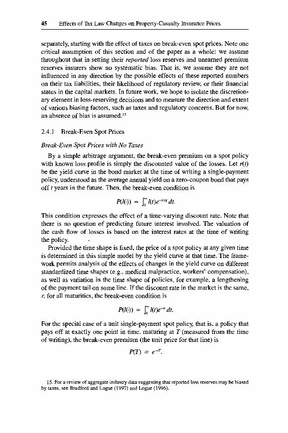
By a simple arbitrage argument, the break-even premium on a spot policy with known loss profile is simply the discounted value of the losses. Let r(t) be the yield curve in the bond market at the time of writing a single-payment policy, understood as the average annual yield on a zero-coupon bond that pays off t years in the future. Then, the break-even condition is
This condition expresses the effect of a time-varying discount rate. Note that there is no question of predicting future interest involved. The valuation of the cash flow of losses is based on the interest rates at the time of writing the policy.
Provided the time shape is fixed, the price of a spot policy at any given time is determined in this simple model by the yield curve at that time. The frame- work permits analysis of the effects of changes in the yield curve on different standardized time shapes (e.g., medical malpractice, workers' compensation), as well as variation in the time shape of policies, for example, a lengthening of the payment tail on some line. If the discount rate in the market is the same, r, for all maturities, the break-even condition is
For the special case of a unit single-payment spot policy, that is, a policy that pays off at exactly one point in time, maturing at T (measured from the time of writing), the break-even premium (the unit price for that line) is
P(r> = e-rT.
15. For a review of aggregate industry data suggesting that reported loss reserves may be biased by taxes, see Bradford and Logue (1997) and Logue (1996).

46 David F. Bradford and Kyle D. Logue
Break-Even Spot Prices with Taxes
In the calculation of the company’s taxable income, gross underwriting in- come consists of premiums earned. A deduction is allowed on account of any increase in the liabilities for future loss payments; that is the loss reserve de- duction. We may start by considering the case in which taxable income is the same as nominal economic income, as defined above. We then consider sig- nificant deviations in the rules from the nominal economic income standard.
Taxes with nominal economic income accounting. When we introduce an in- come tax, we must translate the analysis of cash flows in a single-payment spot policy to net-of-tax terms. If the income tax were actually based on nominal economic income, then the insurance company that issued a policy on break- even terms in the absence of taxes, and fully hedged its position by buying a portfolio of bonds with maturities matching its payment obligations, would not have any income at any point and would not pay any tax. So, under those circumstances, the tax would not affect the equilibrium price of insurance (ex- cept possibly indirectly, through an effect on the level of interest rates). Trans- lated into terms of gross income and deductions, the premium, P, would be included as gross income and the addition to loss reserves of an exactly equal amount (because it is a break-even policy) would be taken as a deduction. Over time, there would be additional deductions for successive loss payments, but they would be matched by equal and opposite changes in the level of loss re- serves. In addition, there would be deductions as the value of discounted loss reserves increased by virtue of the approach to future payout points. These deductions would give rise to negative underwriting income. They would be matched by the yield on the use of funds up until the time of payout, which would give rise to positive investment income, offsetting underwriting losses. So the company’s net taxable income would be zero throughout the life of the contract. (In appendix A, we provide further discussion of the discount rate appropriate for use in setting loss reserves, drawing on the analogy between a single-payment spot policy and a discount bond.)
Taxes with statutory accounting for loss reserves. With statutory accounting for loss reserves, the story is different. The premium comes in as gross income when received, but the simultaneous deduction is of the undiscounted reserve. The in- crease in liabilitjj on a discounted basis that takes place as the time of future pay- ment approaches has no tax consequences. As with nominal economic income accounting, loss payments give rise to a deduction when made, offset by a simul- taneous reduction in the deduction for loss reserves as the stock of undiscounted liabilities for losses incurred is reduced by the amount paid out. So, with statu- tory accounting used for taxpurposes, writing what would be a break-even insur- ance policy in the absence of taxes results in a stream of changes in tax liabilities with positive discounted value to the taxpayer.

47 Effects of Tax Law Changes on Property-Casualty Insurance Prices
In working out the details, we need to take account of the fact that the com- pany will evaluate cash flows on the basis of their after-tax consequences, us- ing the after-tax discount rate. In the case of a constant tax rate, T, the after-tax discount rate applicable to a cash flow t years in the future is (1 - T)r(t).
With statutory accounting, there is a deduction for the undiscounted loss reserve at the time of writing the policy, R(0) = L. The cash flow associated with the policy is thus (1 - T)P + TL at time of issue, followed by the flow -l(t) at subsequent time t consisting of the actual loss payout. Since the payout is deducted and the corresponding increase in loss reserves is included in taxable income, there are no tax consequences at payout time. Denoting the break-even premium under statutory accounting by Ps, it must satisfy the break-even con- dition
(1 - T)P + TL = j;Z(t)e+T)r(f)dt.
Two important characteristics of the impact of taxes using statutory account- ing can be inferred from this break-even condition. First, the tax rate matters. As we show next, the higher the tax rate, the lower the break-even premium, given the term structure of before-tax interest rates. Second, the time pattern of tax rates matters. For example, other things equal, the lower the tax rate anticipated in the future, relative to the time of writing the policy, the lower the break-even premium. Conversely, an anticipated increase in the rate of tax will result in an increase in the break-even premium.
We may contrast this break-even condition with the condition that would apply under nominal economic income accounting, which would involve an initial deduction of the discounted value of the anticipated loss, followed by a stream of deductions for any increase in that discounted value due to the ap- proach of the payment date. (There is a further stream of deductions for the payments themselves that is offset by exactly equal reductions in the stock of reserves.) Letting Rd stand for the discounted value of loss reserves, the cash flow at the time of writing the policy would be (1 - T)P + 7Rd(0), or
(1 - T)P + ?/;Z(t)e-“ d t .
Under our assumption that the losses on the policy are known at the outset, the discounted value of losses remaining to be paid at a time t’ subsequent to the date of issue would be given by
Rd(t’) = ~,~Z(f)e-~f-z’) dt.
The change in discounted reserve is a deduction in calculating nominal eco- nomic income and so would induce a stream of tax savings under a system of nominal economic income taxation. The rate of cash flow at t’ would then be
-Z(t? + .rrRd(t’),

48 David F. Bradford and Kyle D. Logue
where we have used the fact that, net of payouts, the stock of discounted re- serves will grow instantaneously at the rate of interest. Denoting the break- even premium under nominal economic income accounting by P, it must sat- isfy the break-even condition
(1 - -7)P" + ~Rd(0) = j:[l(t') - ~rRd(r')]e-(~-~)"'dr'.
Relying on the discussion in appendix A, we know that this break-even condi- tion implies P = Rd(0).
The relationship between the two break-even premium levels can be ex- pressed in simple form in the case of a single-payment policy. The after-tax cash flow from the break-even premium under statutory accounting must have a discounted (at the after-tax discount rate) value of zero:
p - 7(pS - 1) - e-(I-T)rT = 0
7, (1 - 7)p = e<l-T)rT -
e-u-.i)rr - -7
1 - - 7 p " =
A somewhat startling implication of the calculation is that the break-even loan proceeds to justify a repayment of one after a time period T could actually be negative for large enough values of T, r, or -7. The insurer could afford to pay the policyholder to accept coverage, taking its return in the form of tax savings.
This may be contrasted with the corresponding break-even premium, P", under nominal economic income accounting for tax purposes,
pe = Te-rT.
The ratio of the two
P - eTrT - 7erT P" 1 - 7
- __
depends on the tax rate, the discount rate, and the time to maturity (length of the tail for an insurance policy). If the tax rate is zero or the discount rate is zero or the time to maturity is zero, the two amounts are the same. Increasing the tax rate, the discount rate, or the time to maturity lowers the ratio, that is, lowers the break-even amount under statutory relative to that under nominal economic income accounting. For a high enough discount rate, tax rate, or time to maturity, the competitive premium level is negative, whereas the premium is always positive under nominal economic income accounting.
The relationship between the various parameters (tax rate, discount rate,
49 Effects of Tax Law Changes on Property-Casualty Insurance Prices
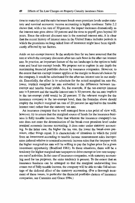
time to maturity) and the ratio between break-even premium levels under statu- tory and nominal economic income accounting is highly nonlinear. Table 2.2 shows that, with a tax rate of 30 percent, the impact increases dramatically as the interest rate goes above 10 percent and the time to payoff goes beyond 10 years. Since the relevant discount rate is the nominal interest rate, it is clear that the recent history of interest rates in the United States includes periods in which the premiums on long-tailed lines of insurance might have been signifi- cantly affected by tax factors.
Aside on tax-exempt interest. In the analysis thus far we have assumed that the rate at which the company discounts after-tax cash flows is the after-tax interest rate. In practice, an important feature of the tax landscape is the option to hold state and local tax-exempt bonds. We propose not to explore in any depth the maximizing financial portfolio choices by insurance companies. However, to the extent that tax-exempt interest applies at the margin to financial choices by the company, it would be substituted for the after-tax interest rate in our analy- sis. Essentially, the effect is to substitute for the actual marginal tax rate the, lower, implicit marginal tax rate embodied in the difference between tax- exempt and taxable bond yields. So, for example, if the tax-exempt interest rate is 8 percent and the taxable interest rate is 10 percent, the tax rate implicit in the tax-exempt yield would be 20 percent. If the relevant margin for the insurance company is the tax-exempt bond, then the formulas above should employ the implicit marginal tax rate of 20 percent (as applied to the taxable interest rate) rather than the statutory tax rate.
An insurance company that is well managed from a tax point of view will, however, try to assure that the marginal source of funds for the insurance busi- ness is fully taxable income. Note that whereas the insurance company’s tax rate does not enter the determination of the break-even premium level under nominal economic income accounting, it does enter under statutory account- ing. In the latter case, the higher the tax rate, the lower the break-even pre- mium, other things equal. It is characteristic of situations in which the yield from an investment according to taxable income measurement rules incorpo- rates deferral relative to nominal economic income rules that the taxpayer with the higher marginal tax rate will be willing to pay the higher price for a given investment opportunity (Bradford 1981). In those situations, there will be a tendency for higher marginal rate taxpayers to drive exempt or low-rate taxpay- ers out of activities. In the case of insurance companies, with statutory account- ing used for tax purposes, the same tendency is present. To the extent that an insurance business can be arranged so that the marginal underwriting loss comes out of fully taxable income, the company will be able to take full advan- tage of the deferral effect of the statutory accounting. (For a thorough treat- ment of these issues, in particular the financial portfolio choices of insurance companies, see Cummins and Grace 1994.)

Table 2.2 Break-Even Premiums for Statutory versus Nominal Economic Income Accounting
7 = 0.1 r = 0.3 T = 0.5
Maturity r=0.05 r = 0 . 1 r=0 .15 r = 0 . 2 r=0.05 r = 0 . 1 r = 0 . 1 5 r = 0 . 2 r=0.05 r = 0 . 1 r=0.15 r = 0 . 2
1 1 .00 1 .00 1 .oo 1 .oo 1 .00 1 .oo 1 .oo 0.99 1.00 1.00 0.99 0.99 3 1 .00 0.99 0.99 0.98 1 .00 0.98 0.96 0.93 0.99 0.97 0.94 0.88 10 0.98 0.93 0.79 0.54 0.95 0.76 0.32 -0.56 0.92 0.58 -0.25 -1.95 20 0.93 0.54 -0.73 -4.41 0.76 -0.56 -5.09 -18.66 0.58 -1.95 -11.12 -39.82
Source: Authors’ calculations.
Nore: Table reports ratio of break-even premium for single-payment policy under statutory accounting relative to that under nominal economic income accounting.

51 Effects of Tax Law Changes on Property-Casualty Insurance Prices
Taxes with statutorily prescribed discounted reserves. As described in section 2.3, since TRA86, insurance companies have been required to use discounted reserves in calculating taxable income. As far as spot policies are concerned, it would be reasonable to describe the post-TRA86 rules as taxing companies roughly on a nominal economic income basis. As described above, however, the rules limit the flexibility of insurance companies to vary the loss profile assumed in calculating income, and they incorporate an assumed interest rate that may be different from the one actually prevailing. To illustrate, suppose the prescribed profile were “too long,” T’ instead of T for our single-payment example, and the interest rate “too low,” r’ instead of r. Then, unlike the case of consistent nominal economic income accounting, the tax rate and interest rates would influence the break-even premium, P. As a consequence, it is nec- essary to model the determination of break-even premiums using an explicit specification of the Treasury discount factors.
2.4.2 From Break-Even Spot Prices to Earned Premiums
The theoretical analysis developed above relates to the economics of a spot policy. A standard policy incorporates a year’s worth of spot policies, paid for at the beginning of the year. To get from spot policy prices to standard policy prices requires discounting the anticipated spot policy amounts. The income tax also affects the relationship between break-even spot prices and break-even standard policies, via the treatment of unearned premium reserves (which was changed in 1986).
Industry data on premiums take the form of amounts earned during the re- porting year. The amount earned during a reporting year constitutes the pro rata portions of premiums on standard policies that commenced during the previous year or that extend into the next accounting year. These amounts may be differentially affected by changes in the rates of tax during these years.
Appendix B describes how we deal with these and many other details in the process of developing the figures presented in the next section, which describes the empirical results.
2.5 Empirical Results
2.5.1 Profiles, Tax Rates, Discount Rates, and IRS Reserve Discount Factors
To implement the formulas derived above we require data on loss profiles, taxes, discount rates, and IRS discount factors (for unpaid loss reserves).
Profiles
A unit loss profile in a line of insurance is assumed to take the form of a sequence of discrete payments, lj , occurring at times, tj, measured from the
52 David F. Bradford and Kyle D. Logue
Table 2.3 Unit Spot Policy Loss Profiles Based on ” I r y Data (percent)
Auto Other Workers’ Medical Farmowners, Tax Year Liability Liability Compensation Malpractice etc.
AY + 0 AY + 1 AY + 2 AY + 3 AY + 4 AY + 5 AY + 6 AY + 7 AY + 8 AY + 9 AY + 10 AY + 11 AY + 12 AY + 13 AY + 14 AY + 15
Total
34.32 30.88 15.03 8.82 4.16 2.13 1.24 0.64 0.23 0.32 0.32 0.32 0.32 0.06 0.00 0.00
100.00
9.20 16.19 14.69 15.13 10.99 8.92 5.11 4.28 2.16 1.02 1.02 1.02 1.02 1.02 1.02 7.23
100.00
25.92 28.61 13.33 1.14 4.41 3.50 1.88 1.73 1.50 0.62 0.62 0.62 0.62 0.62 0.62 7.58
100.00
3.02 9.96
10.45 12.15 9.90 8.27 7.03 6.47 5.13 2.74 2.74 2.74 2.14 2.74 2.14
11.20
100.00
55.14 23.39 7.33 4.75 3.05 2.43 1.05 0.38 0.68 0.32 0.32 0.32 0.25 0.00 0.00 0.00
100.00
Source: Derived from A. M. Best Company (1988).
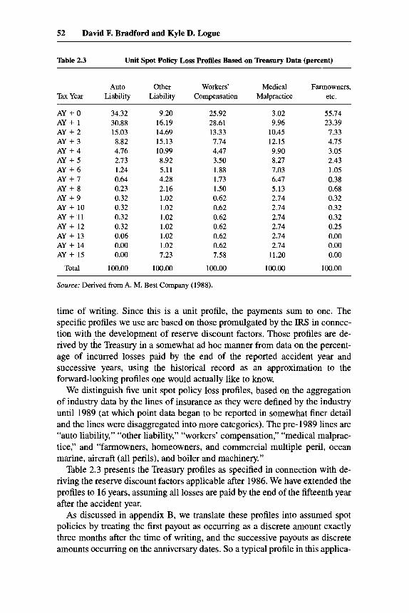
time of writing. Since this is a unit profile, the payments sum to one. The specific profiles we use are based on those promulgated by the IRS in connec- tion with the development of reserve discount factors. Those profiles are de- rived by the Treasury in a somewhat ad hoc manner from data on the percent- age of incurred losses paid by the end of the reported accident year and successive years, using the historical record as an approximation to the forward-looking profiles one would actually like to know.
We distinguish five unit spot policy loss profiles, based on the aggregation of industry data by the lines of insurance as they were defined by the industry until 1989 (at which point data began to be reported in somewhat finer detail and the lines were disaggregated into more categories). The pre-1989 lines are “auto liability,” “other liability,” “workers’ compensation,” “medical malprac- tice,” and “farmowners, homeowners, and commercial multiple peril, ocean marine, aircraft (all perils), and boiler and machinery.”
Table 2.3 presents the Treasury profiles as specified in connection with de- riving the reserve discount factors applicable after 1986. We have extended the profiles to 16 years, assuming all losses are paid by the end of the fifteenth year after the accident year.
As discussed in appendix B, we translate these profiles into assumed spot policies by treating the first payout as occurring as a discrete amount exactly three months after the time of writing, and the successive payouts as discrete amounts occurring on the anniversary dates. So a typical profile in this applica-

53 Effects of Tax Law Changes on Property-Casualty Insurance Prices
Table 2.4 Average Time to Payout by Line
Line Average Time to Payout
(years)
Auto liability 1.57 Other liability 4.38 Workers’ compensation 3.12 Medical malpractice 6.34 Farmowners, etc. 1.17
Source: Authors’ calculations based on data from A. M. Best Company (1988).
tion involves a payout at the .25, 1, 2, . . . , etc. year points. It is immediately apparent from the table that there is considerable variation in the length of the tails of the different lines. Based on our assumed timing, the average times to payout implicit in the data are shown in table 2.4. Referring to table 2.2, show- ing the effect of the difference between statutory and discounted reserve ac- counting for tax purposes, we can see that the only line for which we might look for a significant effect is medical malpractice.
Anticipated Tax Rates
Tax rates have changed from time to time. The break-even premium under statutory accounting depends on the company’s anticipation of future tax rates. Sometimes tax legislation specifies the future course of tax rates. For purposes of this exercise, we assume that companies know the tax rate that will, in fact, apply to the year of writing the policy (the first of two accident years that will be touched by the policy) and for future years believe the tax rates specified in legislation as of the end of the accident year. (We also assume in this paper that companies do not manipulate their loss reserves.) Table 2.5 specifies the tax rates used in our calculations for each year. The rates shown on the diagonal are the rates that actually applied in the years in question. The last column, for 1993, is repeated for all future years required in the calculations.
Discounting
In determining the spot price at any time, discounting is at the then-current term structure of interest rates. The interest rate data that we use are in the form of yields on Treasury securities of different maturities. Although such a yield is derived as an internal rate of return on securities that make periodic coupon payments between issue date and maturity, we treat the rates as applying to zero-coupon bonds with various maturities. So, if the five-year yield is reported as 7 percent, we assume $1 payable in five years can be bought for e-.07*5 = e-.35. The after-tax interest rate applicable to a 40 percent bracket taxpayer would be 4.2 percent. We use the notation r(t) to designate the interest rate applicable to a zero-coupon bond of maturity t . Where the relevant matu- rity does not correspond exactly to a maturity available in the data (e.g., four

Table 2.5 Federal Income Tax Rates Used in Calculating Break-Even Premiums
Tax Rates in Tax Rates Anticipatedin 1976 1977 1978 1979 1980 1981 1982 1983 1984 1985 1986 1987 1988 1989 1990 1991 1992 1993
1976 .48 .48 .48 .48 .48 .48 .48 .48 .48 .48 .48 .48 .48 .48 .48 .48 .48 .48 1977 .48 .48 .48 .48 .48 .48 .48 .48 .48 .48 .48 .48 .48 .48 .48 .48 .48 1978 .48 .46 .46 .46 .46 .46 .46 .46 .46 .46 .46 .46 .46 .46 .46 .46 1979 .46 .46 .46 .46 .46 .46 .46 .46 .46 .46 .46 .46 .46 .46 .46 1980 .46 .46 .46 .46 .46 .46 .46 .46 .46 .46 .46 .46 .46 .46 1981 .46 .46 ,415 .46 .46 .46 .46 .46 .46 .46 .46 .46 .46 1982 .46 .46 .46 .46 .46 .46 .46 .46 .46 .46 .46 .46 1983 .46 .46 .46 .46 .46 .46 .46 .46 .46 .46 .46 1984 .46 .46 .46 .46 .46 .46 .46 .46 .46 .46 1985 .46 .46 .46 .46 .46 .46 .46 .46 .46 1986 .46 .4 .34 .34 .34 .34 .34 .34 1987 .4 .34 .34 .34 .34 .34 .34 1988 .34 .34 .34 .34 .34 .34 1989 .34 .34 .34 .34 .34 1990 .34 .34 .34 .34 1991 .34 .34 .34 1992 .34 .34 1993 .35
Source: Commerce Clearing House, Standnrd Federal Tax Reponer (Chicago, 1996). 1: pP3265.0129-.0139. Note: State tax rates have been ignored.

55 Effects of Tax Law Changes on Property-Casualty Insurance Prices
I I IY._
14.00
+4/1177
+ 10/1/81 -&-a1183
+4/2/84
* 10/1186 + 10/3/88 ! + 10/1/93
1 Year 2 Year 3 year 5 Year 7 Year 10 year 30 year
Maturities
Fig. 2.1 Term structure of interest rates, selected dates Source: Federal Reserve Board and authors' calculations. Note: Average bond yields for various maturities, selected dates. Dates correspond to extrema in the 10-year yield.
years), we use a linear interpolation of the rates reported for the nearest adja- cent maturities.
We calculate spot prices for policies written on 1 April and 1 October (more precisely, the first business days of the second and fourth quarters) each year. The applicable term structures are derived as simple averages of the term struc- tures, compiled on a daily basis by the Federal Reserve Board, during the first and second halves of the year. Figure 2.1 shows the term structure at selected dates (the turning points in the 10-year yield in the constructed time series).
We use the notation a(t) for the after-tax discount factor applied to a cash flow at time point t after the date of issue of a spot policy. These discount factors vary with the date of issue, in part because the term structure of before- tax interest rates varies and in part because the tax rates vary. The applicable tax rates for purposes of determining the break-even premium at any time are those anticipated at that time. Because the discrete payment profile that we use is an approximation to a continuous profile, the applicable tax rate is obtained by averaging over the interval from zero to the time midway to the next discrete payment point. So, for example, if T = 6, and the tax rate is 46 percent for the first year and 40 percent for the next five and a half years, the after-tax discount factor applicable to a cash flow at the six-year point is
(1 - .46) + 5.5(1 - .40) 6.5

56 David F. Bradford and Kyle D. Logue
Note that for this model we assume that the relevant tax rates are not the ones that actually prevailed in all instances. Rather, they are the tax rates that were expected to prevail at the date for which the after-tax discount factor is being derived.
Reserve Discount Factors
The reserve discount factors applied to undiscounted loss reserves for in- come tax purposes after 1986 are those promulgated by the Treasury in 1987 and 1992. The factors provided in 1992 are for the post-1989 definition of lines. For our analysis, we use five of the six lines for which data are available before 1989. For the post-1989 period we have aggregated the more narrowly defined lines into the same five broader lines (auto liability, etc.). The reserve discount factors applied in 1992 and thereafter are obtained by averaging the published IRS factors, using aggregate incurred losses in the disaggregated lines for the year as weights.
2.5.2 Calculated Spot Premiums, 1976-93
Tables 2.6 to 2.10 show the calculated break-even spot premiums in each line of insurance from 1976 through 1993 based on our model in section 2.4. The figures shown are simple averages of the 1 April and 1 October spot policy premiums that we use in the derivation of break-even standard and break-even earned premiums. The tables also show the break-even spot premiums that would have been implied based on statutory accounting (undiscounted loss reserves) and nominal economic income accounting for tax purposes through- out the series of years. For the years up to 1986, the applicable tax law is based on statutojl accounting for loss reserves. After 1986, reserves are discounted for tax purposes. The special fresh-start rules applied in 1986. The column headed “Ratio of P(ATL) to P(NE1)” indicates the influence on the break-even spot premiums of the deviation of the applicable tax law accounting from the nominal economic income accounting applied to ordinary borrowing and lend- ing. After 1986, this ratio also indicates how closely the Treasury’s rules repli- cated nominal economic income accounting. The column headed “Ratio of P(ATL) to P(SA)” indicates the impact of the change in rules in 1986.
Referring to table 2.4, we see that the calculated break-even spot premiums have the expected relationship to the length of the tail in a line. In 1978, for example, the break-even premium under the applicable tax law was 0.9 1 in the farmowners, etc., line (the line with the shortest tail) and 0.55 in the medical malpractice line (the line with the longest tail). The differences were more pronounced in the early 1980s when interest rates were very high by historical standards. In 1981, the break-even price in the farmowners, etc., line was 0.85 and in the medical malpractice line was 0.36.
The difference between break-even prices under statutory accounting and applicable tax law accounting after 1986 also corresponds to the expectations based on the average length of the tails. As expected, the case where the differ- ence is most pronounced is medical malpractice, where the change from undis-

Table 2.6 Break-Even Spot Premiums for Auto Liability, 1976-93
P under P under Nominal P under Ratio of Statutory Ratio of
Economic Income, Applicable Tax P(ATL) to Accounting, P(ATL) to Year P(NE1) Law, P(ATL) P(NE1) P(S.4) P(SA)
1976 1977 1978 1979 1980 1981 1982 1983 1984 1985 1986 1987 1988 1989 I990 1991 1992 1993
0.91 0.91 0.89 0.87 0.85 0.82 0.84 0.86 0.85 0.87 0.90 0.90 0.89 0.88 0.89 0.91 0.93 0.94
0.90 0.90 0.88 0.86 0.84 0.80 0.82 0.85 0.84 0.86 0.81 0.90 0.89 0.88 0.89 0.91 0.93 0.94
0.99 0.99 0.99 0.99 0.99 0.98 0.98 0.99 0.98 0.99 0.90 1 .oo 1 .oo 1 .oo 1 .oo 1.00 1.00 1.00
0.90 0.90 0.88 0.86 0.84 0.80 0.82 0.85 0.84 0.86 0.88 0.88 0.88 0.88 0.88 0.90 0.92 0.93
1 .oo 1 .oo 1 .oo 1 .oo 1 .oo 1 .oo 1 .oo 1 .oo 1 .oo 1 .oo 0.92 1.02 1.01 1.01 1.01 1.01 1 .oo 1 .oo
Source: Authors' calculations.
Table 2.7 Break-Even Spot Premiums for Other Liability, 1976-93
P under P under Nominal P under Ratio of Statutory Ratio of
Economic Income, Applicable Thx P(ATL) to Accounting, P(ATL) to Year P(NEI) Law, P(ATL) P W I ) P(SA) P(SA)
1976 1977 1978 1979 1980 198 1 1982 1983 1984 1985 1986 1987 1988 1989 1990 1991 1992 1993
0.76 0.76 0.73 0.70 0.66 0.61 0.63 0.68 0.65 0.69 0.76 0.74 0.73 0.72 0.73 0.76 0.79 0.82
0.73 0.73 0.68 0.65 0.60 0.53 0.56 0.62 0.58 0.64 0.55 0.73 0.72 0.72 0.73 0.76 0.79 0.81
0.96 0.96 0.93 0.94 0.91 0.87 0.89 0.92 0.90 0.92 0.73 0.99 1 .oo 1 .oo 1 .oo 1 .oo 1 .oo 1 .oo
0.73 0.73 0.68 0.65 0.60 0.53 0.56 0.62 0.58 0.64 0.68 0.69 0.70 0.70 0.70 0.73 0.77 0.80
1 .oo 1 .oo 1 .oo 1 .oo 1 .oo 1 .oo 1 .oo 1 .oo 1 .oo 1 .oo 0.81 1.07 1.04 1.04 1.04 1.03 1.02 1.02
Source: Authors' calculations.

Table 2.8 Break-Even Spot Premiums for Workers’ Compensation, 1976-93
P under P under Nominal P under Ratio of Statutory Ratio of
Economic Income, Applicable Tax P(ATL) to Accounting, P(ATLj to Year P(NEI) Law, P(ATL) P W I j P(SA) P(SAj
1976 1977 1978 1979 1980 1981 1982 1983 1984 1985 1986 1987 1988 1989 1990 1991 1992 1993
0.83 0.84 0.81 0.79 0.76 0.73 0.75 0.78 0.76 0.79 0.83 0.82 0.81 0.81 0.81 0.83 0.86 0.87
0.81 0.81 0.78 0.75 0.72 0.67 0.69 0.74 0.71 0.75 0.67 0.82 0.81 0.81 0.81 0.83 0.86 0.87
0.97 0.97 0.96 0.96 0.94 0.92 0.93 0.95 0.94 0.95 0.81 1 .oo 1 .oo 1 .oo 1 .oo 1 .oo 1 .oo 1 .oo
0.8 1 0.81 0.78 0.75 0.72 0.67 0.69 0.74 0.71 0.75 0.78 0.78 0.79 0.79 0.79 0.81 0.84 0.86
1 .oo 1 .oo 1 .oo 1 .oo 1 .oo 1 .oo 1 .oo 1 .oo 1 .oo 1 .oo 0.86 1.05 1.02 1.03 1.03 1.02 1.02 1.02
Source: Authors’ calculations.
Table 2.9 Break-Even Spot Premiums for Medical Malpractice, 1976-93
P under P under Nominal P under Ratio of Statutory Ratio of
Economic Income, Applicable Tax P(ATLj to Accounting, P(ATLj to Year P(NE1) Law, P(ATLj P ( N W P(SAj PGA)
1976 1977 1978 1979 1980 1981 1982 1983 1984 1985 1986 1987 1988 1989 1990 1991 1992 1993
0.66 0.67 0.63 0.59 0.55 0.49 0.5 1 0.56 0.53 0.58 0.66 0.64 0.62 0.63 0.63 0.66 0.69 0.73
0.61 0.62 0.55 0.52 0.45 0.36 0.40 0.47 0.42 0.49 0.39 0.63 0.62 0.62 0.63 0.66 0.69 0.73
0.92 0.92 0.88 0.87 0.82 0.73 0.77 0.83 0.79 0.85 0.59 0.98 0.99 1 .oo 1 .oo 1 .oo 1 .oo 0.99
0.61 0.62 0.55 0.52 0.45 0.36 0.40 0.47 0.42 0.49 0.55 0.56 0.58 0.58 0.58 0.62 0.66 0.70
1 .oo 1 .oo 1 .oo 1 .oo 1 .oo 1 .oo 1 .oo 1 .oo 1 .oo I .oo 0.71 1.13 1.07 1.07 1.07 1.06 1.05 1.04
Source: Authors’ calculations.

59 Effects of Tax Law Changes on Property-Casualty Insurance Prices
Table 2.10 Break-Even Spot Premiums for Farmowners, etc., 197693
P under P under Nominal P under Ratio of Statutory Ratio of
Economic Income, Applicable Tax P(ATL) to Accounting, P(ATL) to Year P(NEI) Law, P(ATL) P(NE1) P(SA) P(SA)
1976 1977 1978 1979 1980 1981 1982 1983 1984 1985 1986 1987 1988 1989 1990 1991 1992 1993
0.93 0.93 0.92 0.90 0.89 0.86 0.88 0.90 0.89 0.91 0.93 0.92 0.92 0.91 0.92 0.93 0.95 0.95
0.93 0.93 0.91 0.89 0.88 0.85 0.87 0.89 0.88 0.90 0.84 0.93 0.92 0.91 0.92 0.93 0.95 0.95
1.00 1 .00 0.99 0.99 0.99 0.98 0.99 0.99 0.99 0.99 0.91 1.01 1 .oo 1 .00 1 .oo 1 .oo 1 .00 1.00
0.93 0.93 0.91 0.89 0.88 0.85 0.87 0.89 0.88 0.90 0.91 0.91 0.91 0.91 0.91 0.93 0.94 0.95
1 .00 1 .00 1 .00 1 .00 1 .oo 1 .00 1 .00 1 .00 1 .oo 1 .oo 0.92 1.02 1.01 1.01 1.01 1 .00 1 .oo 1 .00
Source: Authors’ calculations.
counted to discounted loss reserves accounts for a difference of 13 percent in the break-even *price in 1987, declining to a roughly 4 percent difference in 1993. The impact of the fresh-start rules in 1986 (which gave an extra tax boost to loss reserves established in 1986 and earlier) meant that for that year the tax law change reduced the break-even price below what it would have been under statutory accounting. The particularly large effect of the tax law change in 1987 reflects in part the impact of the declining rate of tax from 1986 to 1988. Under statutory accounting for tax purposes, a declining rate of tax between the receipt of premium and the policy payout results in a lower break-even premium. The pattern of declines in the impact of tax reform on break-even premiums after 1987 presumably results from declining interest rates (at a zero rate of interest the two should be the same) since there were no major changes in the tax rates after that point.
Comparing the columns of break-even prices under nominal economic in- come accounting for tax purposes with the effect of the actual tax law in the period from 1987 onward (i.e., after the fresh-start rule had ceased to have any influence), we see that the two are very close. The ratios are essentially one throughout, for all lines, suggesting the Treasury succeeded in implementing the presumed objective of the 1986 shift to discounted loss reserves.

60 David F. Bradford and Kyle D. Logue
2.5.3
In getting to the break-even earned premiums, we calculated break-even standard policy premiums in each line of insurance for 1 April and 1 October from 1976 through 1993. The difference between these premiums and the spot premiums presented above is that the standard policy premiums incorporate the effect of changes in the treatment of unearned premium reserves (a minor effect) and bring to an earlier time point the effect on premiums of changes in interest rates and tax rules. Thus a premium on a policy written on 1 October 1986, incorporates the effect of tax changes manifested in break-even spot premiums during most of 1987.
2.5.4 Predicted Break-Even Premiums versus Actual Earned Premiums, Accident Years 1977-93
Under competitive conditions, the opportunity for profit from all sources, including tax saving, will tend to be driven to zero. Thus we assume that the tax saving is “passed along” to the buyer of the policy in the form of a reduced premium. To make the comparison of the calculated break-even premiums with industry data, we make use of the break-even earned premium concept dis- cussed above. Table 2.11 presents these premiums, for accident years 1977-93 (1976 is lost in the derivation of earned premiums), together with the unit earned premiums implicit in industry data for these accident years, interpreted as the inverse of the loss ratio reported at the end of each accident year. For each line of insurance, there are two columns, one showing the break-even earned premium (“B-E Earned P”) calculated from our model and one showing the ratio of earned premiums per dollar of losses incurred (“lhndustry Loss Ratio”) registered in data for the industry for the year in question. So, for ex- ample, our calculated average of the break-even premiums for the unit standard policies contributing to earned premiums in the other liability line in 1985 was 0.58. The ratio of earned premiums to losses incurred in that line in that year was 0.81. The observed average “price” was higher than would be predicted by our calculation.
In evaluating these figures, one needs to keep in mind that our calculations are highly stylized, neglecting risk premiums in the discount rates, for ex- ample. We would hope to see a relationship between the calculated and the observed prices, not necessarily equality. One important influence on the em- pirical ratios is the fact that industry data relate to premiums earned gross of the cost of acquiring the policies, whereas our calculations would apply to premiums net of acquisition costs. Best’s reports the following figures for “other underwriting expenses” incurred, as a ratio to premiums earned, in the reporting years: 1990 (26.36 percent), 1989, (26.25 percent), 1988 (25.97 per- cent), 1987 (25.95 percent), and 1986 (26.77 percent). Data disaggregated by line, available for 1990, are shown in table 2.12.
To permit more ready comparison of the relationship between calculated
Calculated Standard Policy Premiums, 1976-93
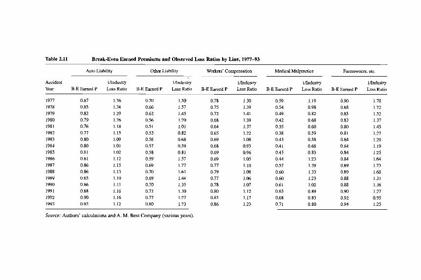
Table 2.11 Break-Even Earned Premiums and Observed Loss Ratios by Line, 1W7-93
Auto Liability Other Liability Workers’ Compensation Medical Malpractice Farmowners, etc.
lfindustry Accident Ifindustry Ifindustry lhdustry lhdustry Year B-E Earned P Loss Ratio B-E Earned P Loss Ratio B-E Earned P Loss Ratio B-E Earned P Loss Ratio B-E Earned P Loss Ratio
1977 1978 1979 1980 1981 1982 1983 1984 1985 1986 1987 1988 1989 1990 1991 1992 1993
0.87 0.85 0.82 0.79 0.76 0.77 0.80 0.80 0.81 0.81 0.86 0.86 0.85 0.86 0.88 0.90 0.92
1.36 1.34 1.29 1.26 1.18 1.15 1 .G9 1.01 1.02 1.12 1.15 1.13 1.10 1.11 1.16 1.16 1.12
0.70 0.66 0.62 0.56 0.51 0.53 0.58 0.57 0.58 0.59 0.69 0.70 0.69 0.70 0.73 0.77 0.80
1.50 1.57 1.45 1.20 1.01 0.82 0.68 0.59 0.81 1.57 1.77 1.61 1.44 1.35 1.30 1.27 1.23
0.78 0.75 0.72 0.68 0.64 0.65 0.69 0.68 0.69 0.69 0.77 0.79 0.77 0.78 0.80 0.83 0.86
1.30 1.39 1.41 1.39 1.37 1.22 1.08 0.93 0.96 1.05 1.10 1.08 1.06 1.07 1.12 1.17 1.23
0.59 0.54 0.49 0.42 0.35 0.38 0.43 0.41 0.43 0.44 0.57 0.60 0.60 0.61 0.63 0.68 0.71
1.19 0.98 0.82 0.68 0.60 0.59 0.58 0.68 0.83 1.23 1.39 1.33 1.23 1.02 0.89 0.83 0.80
0.90 0.88 0.85 0.83 0.80 0.81 0.84 0.84 0.84 0.84 0.89 0.89 0.88 0.88 0.90 0.92 0.94
1.70 1.72 1.52 1.37 1.43 1.27 1.20 1.19 1.25 1.64 1.73 1.60 1.31 1.36 1.27 0.95 1.25
Source: Authors’ calculations and A. M. Best Company (various years).

62 David F. Bradford and Kyle D. Logue
Table 2.12 Other Underwriting Expenses by Line, 1990
Ratio of “Other Underwriting
Expenses” Incurred Premiums Written Other Underwriting to Premiums in 1990 Expenses
Line Written in 1990 (thousand $) (thousand $)
Auto 23.9 60,042,447 14,374,550 Other liability 26.3 17,217,566 4,528,220 Workers’ compensation 17.6 30,957,411 5,448,504 Medical malpractice 15.5 4.01 4,622 622,266 Farmowners, etc. 34. I 44,032,383 15,OO2,167
Source: A. M. Best Company (1991).
1.40
1.20
3 1.00
4 D 0.80 s
‘I 0.60
{ 0.40
0.20
$ 4
B
m
0.00
-=-Inverse Loss Ratio
t 76% of Inverse Loss Ratio
* Break-Even Earned Premiums, SA
Fig. 2.2 Auto liability: break-even earned premium and inverse loss ratio,
Source: Authors’ calculations and A. M. Best Company (various years). 1977-93
and empirical prices, we present in figures 2.2 to 2.6 plots of normalized break- even prices and unit earned premiums in the data for the five lines. For each line of insurance four lines are graphed, plotting the break-even earned pre- mium (“Break-Even Earned Premium,” our calculated amount), the break-even earned premium with statutory accounting (“Break-Even Earned Premium, SA,” also calculated, showing what the break-even premium would have been under continuation of the pre-1986 tax law), the estimated average unit pre- mium in the industry data (“Inverse Loss Ratio”), and the same average unit

o.20 t
+Inverse Loss Ratio
+74% of Inverse Loss Ratii
-x- Break-Even E d Premiums, SA
Time
Fig. 2.3 Other liability: break-even earned premium and inverse loss ratio,
Source: Authors’ calculations and A. M. Best Company (various years). 1977-93
I 1.40
0 .-
! 1.20 s g 1.00 0
9 $ 0.80 ‘B
0.60 I b
Time
-o- Break-Even E d Premium
+Inverse Loss Ratio
+82% of Inverse Loss Ratio
-n- Break-Even E d Premiums, SP
Fig. 2.4 ratio, 1977-93 Source: Authors’ calculations and A. M. Best Company (various years).
Workers’ compensation: break-even earned premium and inverse loss

1.40
1.20
8
8 cl
[ 0.80
.- d
d, 1.00
3
.- 5 i o.60 I $ 0.40
6
9
1 0.40
0.20
i
0.007
6 Break-Even Earned Premium
-n- Inverse Loss Ratio
t 84% of Inverse Loss Ratio
-n- Break-Even Earned Premium, SA
~~
--
I ~ : I : : ~ ! ; I ! : : I :
Fig. 2.5 Medical malpractice: break-even earned premium and inverse loss ratio, 1977-93 Source: Authors’ calculations and A. M. Best Company (various years).

65 Effects of Tax Law Changes on Property-Casualty Insurance Prices
premium deflated by the acquisition cost, represented by the ratios of “other underwriting expenses” to premiums written in 1990, assumed constant throughout (“X% of Inverse Loss Ratio”). The two key graphs from the point of view of assessing the predictive power of the calculated break-even prices on the industry results are “Break-Even Earned Premium” and “X% of Inverse Loss Ratio.” For the short-tailed lines (auto liability and farmowners, etc.), the two graphs arguably track reasonably closely. For the longer tailed lines, for which the discount rate is much more important, the industry data display large variation relative to the path of the calculated break-even prices and generally lie above the calculated levels. Taking the industry loss reserve data at face value, they reveal the highly risky nature of the long-tailed insurance lines. Except for the very longest tailed line, medical malpractice, the variation in the calculated prices (due, mainly, to variation in interest rates) is very small relative to the variation in the industry results.
Finally, the comparison of the two calculated price graphs (“Break-Even Earned Premium” and “Break-Even Earned Premium, SA”) allows an assess- ment of the importance of changes in tax rules as an explanatory factor in the time series of industry results. The graphs suggest that the impact of the changes in tax law in 1986 was small relative to the other factors that influence the average level of industry prices.
2.6 Conclusion
One bottom-line conclusion of our investigation is that the effect of changes in tax law is small relative to the other forces that bear on variation in the average price of property-casualty insurance. The other major conclusion, taken from the tables of break-even spot premiums, is that the 1986 reforms could account for an increase in the predicted price of insurance ranging from next to nothing for the very short tailed lines to 5 or 6 percent in the longest tailed line, medical malpractice. If the 1986 reforms are understood as an ex- cise tax increase on long-tailed property-casualty insurance, perhaps the size of the predicted price effect is not a negligible amount, even if it is not large relative to the annual variation in the industry’s results.
Appendix A Loss Reserve Discounting with Taxes
In the presence of taxes, the appropriate discount rate for the company to use in evaluating after-tax cash flows is the after-tax rate of interest in the market. This is because the after-tax rate of interest expresses the opportunity available to the company to exchange dollars in one period for dollars in another. The

66 David F. Bradford and Kyle D. Logue
discount rate applied to the anticipated losses in deriving the reserves used in calculating nominal economic income is, however, the before-tax interest rate.
To explain why this is so, consider an analogy with a company’s writing an insurance policy: floating a zero-coupon bond. The proceeds of the borrowing are analogous to the premium on the insurance policy. The single payment on the bond at maturity corresponds to tile payoff on a single-payment insurance policy. The analogy of the sale of a policy by an insurance company with a loan from policyholder to the company has been noted by others (see, e.g., Cummins and Grace 1994).
The analogue to treating the premium as “gross income” of the insurance company would be treating the proceeds of the borrowing as gross income. There would, however, be an immediate deduction of the discounted value of the payment anticipated at maturity. Subsequently, as the time for the company to repay the loan approached, its liability, the discounted value of its repayment obligation, would grow. In the income calculation, this growth in liability would be allowed as a deduction (it is simply accruing interest). Finally, at maturity, the company would pay off the loan, taking a deduction for the amount paid, but taking into income the value of the liability, in equal amount, that it takes off its books at that point.
Keeping the analogy with the unit single-payment spot policy, let the face value of the discount bond be one, payable at time T after the date of issue, time 0. Let r be the rate of interest, and T the tax rate. Finally, let A be the amount received by the issuing company. The cash flow of the company at the moment of issuing the bond consists of the proceeds received, A, less the tax on A, treated as gross income, and plus the tax saving due to the deduction of the discouflted (at r) value of one, payable T years in the future. (Note: In general, in this paper we treat taxes as though assessed and paid continuously.) Subsequently, the company obtains a deduction for the growth in value of its repayment obligation under the bond, so there is a stream of tax savings. At maturity, the company pays one and takes a deduction of this amount in the calculation of income for tax purposes (corresponding to the inclusion as gross income of the premium). This deduction is, however, balanced by an equal inclusion in income of the elimination of the accrued value of the liability for payment, corresponding to the write-down of loss reserves in the insurance context. So there is no tax consequence of payoff at maturity. This three-part after-tax cash flow-a lump sum received (net of tax), a flow of tax savings, and a lump sum paid-will be discounted by the company at the after-tax interest rate. It remains to show that the break-even value of A is simply the payoff, one, discounted to time 0 at the before-tax rate of interest.
The break-even condition is that the stream of net after-tax cash flows have a discounted (at the after-tax rate of interest) value of zero:
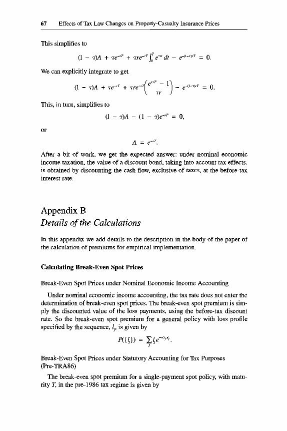
67 Effects of Tax Law Changes on Property-Casualty Insurance Prices
This simplifies to
We can explicitly integrate to get
This, in turn, simplifies to
(1 - 7)A - (1 - 7)e-rT = 0,
or
A = e-rT.
After a bit of work, we get the expected answer: under nominal economic income taxation, the value of a discount bond, taking into account tax effects, is obtained by discounting the cash flow, exclusive of taxes, at the before-tax interest rate.
Appendix B Details of the Calculations
In this appendix we add details to the description in the body of the paper of the calculation of premiums for empirical implementation.
Calculating Break-Even Spot Prices
Break-Even Spot Prices under Nominal Economic Income Accounting
Under nominal economic income accounting, the tax rate does not enter the determination of break-even spot prices. The break-even spot premium is sim- ply the discounted value of the loss payments, using the before-tax discount rate. So the break-even spot premium for a general policy with loss profile specified by the sequence, 4, is given by
Break-Even Spot Prices under Statutory Accounting for Tax Purposes (he-TRA86)
rity T, in the pre-1986 tax regime is given by The break-even spot premium for a single-payment spot policy, with matu-

68 David F. Bradford and Kyle D. Logue
(1 - 7)P(T) + 7 = e-('+fl'77
provided there is no anticipated change in the tax rate. If a change in tax rate is anticipated, the exponent in the discount factor on the right-hand side is modified, as discussed in the body of the paper.
The break-even spot premium for a general policy with loss profile specified by the sequence 1, (to simplify, again assuming no change in the applicable tax rate) is given by
(1 - T ) P ( { < } ) + T = ~ < e + T ) f l $ ) ~ . j
Break-Even Spot Prices with Discounted Loss Reserves (Post-TRA86)
For policies written after 31 December 1986, prescribed reserve discount factors are applied to loss reserves at year end, the factors depending on the line of insurance. As we have done in the analysis of break-even prices with statutory accounting, we assume that tax liabilities are calculated continuously so that the gross premium income and initial loss reserve deductions are effec- tively realized immediately on writing a new spot policy. In the case of dis- counted loss reserves, there is a sequence of additions that result from the passing of time.
To illustrate the way the discount factors enter the break-even conditions, let the reserve discount factors applied at the moment of writing, on the first anniversary, and so on, be denoted fo, f,, f,, etc. For a single-payment spot policy, the factors are increasing, as the undiscounted loss reserve remains con- stant until the moment of payment. The discount factors thus reflect the ap- proach in time of the single payment. For a more general policy, the discount factors may decrease, as the effective length of the remaining tail of payments may increase as the early payments are realized. In the case of a unit single- payment spot policy with maturity T (taken to be an integer), assuming a con- stant tax rate, the break-even condition is
(1 - T)P(Z') + T - + T(X - fg)e+l-')fll) + 7(f, - jJe+1-T)f12)2 + . . .
On the left-hand side are included the tax savings due to the successive addi- tions to loss reserves owing to the passing of time. The last term on the left is the tax saving due to any divergence of the last value of the discounted reserve from unity. On the right-hand side is the discounted loss payment.
If the tax rate is varying over time, the value of the deductions and the after- tax discount factors will be affected in the manner discussed in general terms above and spelled out in detail below.
Using Line-Specijc Reserve Discount Factors
If we were provided with the appropriate discount factors for each possible single-payment policy, we could calculate the break-even premium for a gen-

69 Effects of Tax Law Changes on Property-Casualty Insurance Prices
era1 spot policy, with loss profile specified by a sequence of loss payments, by treating each separate payment as a single-payment spot policy, using the for- mula above, then adding the premiums together.
For our purposes, there are two problems with the discount factors provided by the IRS. First, they are designed to apply to an aggregation of policies over a one-year period, rather than spot policies. Second, they apply to a given line, rather than to single-payment spot policies.
The first reserve discount factor specified by the IRS is to be applied to the reserve in the relevant line on the company’s books at the end of the initial accident year. Conceived of in terms of an aggregate of spot policies, this re- serve includes amounts remaining to be paid on policies ranging in age from one year (written on 1 January) to zero years (written on 31 December). The IRS reserve discount factor is based on a spot policy written on 1 July. It is thus “too close” to the loss payout (i.e., too high) compared to the factor appro- priate for the actual payout pattern associated with a newly written spot policy. Compared with the policy written a year earlier, the IRS factor is six months “too far” from the actual payouts (so, too low). As an approximation, we apply this factor to the undiscounted loss reserve (equal to one for a unit policy) associated with a newly written spot policy. That is, we allow an immediate deduction of this first factor at the time of writing a unit spot policy.
The development of the further reserve deductions, associated with the grad- ual increase in the reserve discount factor as the payout time approaches, is complicated by the fact that the IRS reserve discount factors are specified by line of insurance, rather than by timing of single payments. As will be dis- cussed, because of the way cumulative loss data are reported, we approximate the loss profile in a given line as involving discrete loss payments at the three- month point from the date of writing a spot policy, followed by payouts on the anniversary dates. In our treatment of the payout profiles as known with cer- tainty, an equal reduction in the (undiscounted) unpaid loss reserve corre- sponds to each loss payout.
The taxable income calculation brings into income the decline in discounted reserves during the year and allows a deduction of the loss payments during the year. Using the notation L(t) for the Cumulative payments up to and including t , the path of undiscounted reserves for a unit policy is given by 1, (1 - L( l)), (1 - L(2)), etc., at the outset and at successive anniversaries. The path of dis- counted reserves is thus given byf,,f,(l - L(l)),f2(l - L(2)), etc. The taxable income associated with a unit policy is thus P -f, at the moment of writing, &-f,(l -L(l))-L(l)inthefirstyear,f,(l -L(l))-f2(l -L(2))-(L(2)-L(l)) in the second year, and so on. In the last year, the taxable income will be
The IRS cumulative loss profiles specify amounts regarded as paid as of six months from the time of writing the policy in a line, 1.5 years, etc., through an assumed “last year.” Let the cumulative amount paid out at these successive points be denoted F,, F,, etc., through F,. For a unit policy, F , = 1. We think
f,,(l - L ( T - 1))-(1 - L ( T - 1)).
70 David F. Bradford and Kyle D. Lope
of these cumulative payouts as derived from constant payout rates over the interval in question. So the rate of loss payout would start at 2F0 for the first six months of the policy life (the factor of two comes from the fact that the interval to the first cumulation point is just half a year). The loss payout would continue at the rate of F, - Fo for the period from .5 years to 1.5 years, at the rate of F2 - F3 for the period from 1.5 years to 2.5 years, etc.
The constant rates are in turn converted to discrete payments at the mid- points of the various intervals. So the first loss payout is taken to be Fo at the .25-year (three-month) point. The second payout is F, - Fo at the midpoint between .5 years and 1.5 year, that is, at the one-year point. And so on. The last payout is FT - FT-, = 1 - FT-, at the T-year point.
The formulas above assume constant tax rates. In the calculations, as sum- marized in table 2B.1, the after-tax discount factors, a(t), are based on the actual anticipated tax rates, which are also used to determine the projected tax consequences of future cash flows.
Break-Even Spot Prices after TRA86: The Transition
These descriptions apply to spot policies written in worlds governed entirely by either the pre- or post-TRA86 rules. It remains to determine the break-even price for a policy that crossed the boundary. Consider, for example, a single- payment spot policy written on 1 April 1986. An immediate deduction of the undiscounted loss reserve would apply at the moment of writing. Then, as of 1 January 1987, it would begin to accrue additional deductions for the accruing value of its discounted reserve as of that date. These deductions would continue until the maturity date, at which point, ideally, the discounted reserve would equal the payoff amount. The tax effect of the loss deduction would, as usual, be offset by the write-down of the reserve associated with the policy.
The fresh-start rule meant that, in effect, companies received tax deductions of more than 100 percent of the amount of the losses. For policies that had already been written, this meant a gain to the companies, but it had no incentive effect, no effect on the break-even prices. But to the extent a company could anticipate the fresh-start rule, there would be a downward effect on the break- even price.
For purposes of this exercise, we assume that the fresh-start rules were built into break-even premiums starting 1 January 1986. As will be discussed below, in application, we calculate spot prices as of the first day of the second and fourth quarters each year. So the fresh-start rules need to be taken into account for the two prices calculated for 1986.
For the single-payment spot policy with maturity Z written on 1 April 1986, the fresh-start rule meant an immediate deduction of one and then a stream of deductions, which we treat as occurring on the anniversary dates, along the lines just discussed for the policy entirely in the post-TRA86 regime. For the case of a constant tax rate, the break-even condition is then

Table 2B.1 Unit Spot Policy Cash Flows, Post-TRAM Rules
Time (relative to issue Payments/Receipts date of spot policy) Other Than Taxes Taxable Income Applicable Tax Rate Applicable Discount Factor
0
1 2
.25

72 David F. Bradford and Kyle D. Logue
The difference from the previous formula is that the first reserve deduction is worth T, instead of ~f,.
Summing Up the Cases
In all we calculate break-even spot prices under three sets of assumptions about taxes: Under statutory accounting, the unit loss is deducted at the mo- ment of writing the policy. In terms of table 2B.1, the effect is to setx = 1 for all i . Under applicable tax law, the same is true until 1986. From 1987 onward, the discount factors,A, prescribed by the IRS apply. For 1986, the same dis- count factors apply for cash flows in 1987 and later, but taxable income in the 1986 year of writing the policy (but not on the anniversary) is based on& = 1. Under nominal economic income accounting the price is based on the cash flow of premium and payments only, without regard to taxes, using the discount factors based on before-tax interest rates.
Calculating Standard Policy Premiums
Accounting for the Time Structure of an Insurance Policy
In order to calculate break-even premiums to compare with data we need to take account of the fact that the usual insurance policy covers events that occur during a specified period, usually a year, commencing with the date of issue. The premium is generally payable at the beginning of the policy year. At the moment of writing, there will have been no losses incurred, and so no addition to the loss reserve. As time passes, losses accumulate, and the company books incurred losses, basing its accounts on actual information (e.g., claims actually filed) and experience with similar insurance policies in the past. At the moment of writing the policy the company does acquire an asset, the premium paid or receivable, to which corresponds the liability to provide coverage for the period covered. At the moment of writing, the coverage for which the premium is payment has yet to be delivered, so the liability to provide that coverage is carried on the books as an "unearned" premium reserve. By convention, the premium on a policy is treated as "earned" ratably over the policy period.
The significance of these accounting details is, in part, the necessity they reveal of dealing with the distinction between premiums written, which are taken into income for both tax and regulatory purposes, and the set-aside for premiums not yet earned, which is allowed for in tax and statutory accounting. The tax rules with respect to unearned premium reserves were changed in TRA86, and we need to incorporate this change into our calculations.
A second reason for undertaking an explicit analysis of the timing of premi-

73 Effects of Tax Law Changes on Property-Casualty Insurance Prices
ums received and earned is that the premium determined in our calculations will actually be earned over a period of time that will generally include more than one taxable year. Since tax rules generally apply to whole calendar years, the price of a policy that will span 1 January will need to incorporate the chang- ing rules on the income as well as the deduction (loss reserves) side.
A third reason is that industry data we examine relate to premiums earned, reported by accident year. Those premiums earned will be in part the playing out of policy years that began the year before the accident year in question and in part the initial phase of policies written during the accident year. If premi- ums were separately calculated and reported for coverage within a particular calendar year (so that a typical one-year policy written on 1 September 1987 would have a premium for the period through 31 December 1987 and a pre- mium for the period 1 January through 31 August 1988), this would not create problems for us. But the convention that premiums are earned ratably over the policy period means that data on earned premiums may show a different pat- tern than year-by-year calculations would imply.
To illustrate, suppose that the theory tells us that in some isolated year, say 1983, the tax rules imply a very high spot premium relative to all other years. A company writing a one-year policy on 1 September 1982 could be thought of as writing two policies, a low-priced one for the last four months of 1982 and a high-priced one for January-August 1983. There will be just one price, however, intermediate between the two, which will be reported (and taxed) partly in 1982 and partly in 1983. Premiums earned for accident year 1982 will thus include some of the effect of the 1983 tax rule changes (and thus be higher than would be predicted based just on 1982 tax rules), while the premiums earned in the 1983 accident year will include a residual influence of the pre- 1983 rules.
The analysis thus far of break-even spot premiums assumed that, at a given moment, the insurance company acquires a liability to make a known sequence of loss payments over time and inquired into the up-front payment that would make this a break-even proposition, taking into account the tax-implied tax payments. The fact that, in actuality, the company typically sells a whole year’s worth of spot policies at once influences the way we need to interpret data on loss reserves and earned premiums and, because of details of the treatment of the premium payment under the tax law, it affects the break-even formulas as well.
For example, when an insurance company sells a medical malpractice policy for a term of one year commencing on 1 September 1988, it knows that on 1 September, with certain probabilities, an event will occur that will give rise to a claim and that the result will be a certain series of loss payments and ex- penses in the future. It knows the same for 2 September, and so on. The pre- mium it charges for this one-year policy is to pay for these 365 one-day poli- cies. For present purposes, we continue to dispense entirely with the risk aspect
74 David F. Bradford and Kyle D. Logue
of this situation, and we imagine the company as taking on 365 known liabili- ties. Thus one of the liabilities, incorporated in the premium as of 1 September, is to provide a stream of payments, starting 6 December, with the characteristic medical malpractice profile.
In the absence of taxes, this nicety would not matter much. The one-year premium would simply be the discounted value of the 365 spot premiums on the daily policies. With taxes, the nicety could matter because the spot prices may themselves vary over the year as the result of variation in the interest rates or in the tax rules themselves. But the tax system, in effect, treats the spot price as uniform throughout the policy year. (The single annual premium is treated as “earned” in proportion to the fraction of the policy year that has elapsed.)
To explore this issue, consider the case of a loss payment profile on the spot policy whereby the first loss payment occurs .5 years after the covered day. After that, payments occur at one-year intervals. The loss reserve is set up on the date the policy is written. The new question to be considered is how tax law changes as of 1 January affect the analysis.
For a policy written after 1 July, the loss payments are shifted by one year, in terms of the applicable tax law, compared with the policy written before 1 July. So if interest rates are unchanged, for the case of spot premiums (im- plying no unearned premium problem) there will be one premium before 1 July and another one after 1 July. In going from the second half of one year to the first half of the next, there may be a difference in spot premium (even given constant interest rates), owing to the taxation of the premium, net of loss reserve. This is why we calculate two spot prices for each year, using the inter- est rate conditions as of the beginning of April and October.
Calculating Break-Even Standard Policy Prices
The break-even premium on a standard policy is the amount the company must receive to finance the flow of premiums on the embedded implicit spot policies over the year. So the starting point for calculating it is the calculation of spot premiums.
We assume that, looking forward from 1 April, the company correctly antici- pates the spot premiums that will prevail on 1 October of the current year and on 1 April of the next year. Our calculated break-even standard premium on 1 April is based on the approximation of a single spot policy issued on 1 July of the current year and 1 January of the next year. The 1 July spot premium is the average of the spot premiums on 1 April and 1 October. The 1 January spot premium is the average of the 1 October spot premium and next year’s 1 April spot premium. These hypothetical spot premiums (1 July and 1 January) are discounted to 1 April.
The analogous procedure is used to derive the 1 October standard premium each year.
The detail to be resolved is the discount rate to apply to these spot premiums in getting to the standard premiums.

75 Effects of Tax Law Changes on Property-Casualty Insurance Prices
Table 2B.2 Discounting from Spot to Standard Premium before TRA86
After-Tax Cash Flows 1 October 1983 30 September 1984
Up front X - 7(9/30/84)*~ spot y - 'r(9/30/84)*y
Standard Policy Prices with No Taxes
In the absence of taxes, the break-even premium on a standard policy start- ing at a particular time would simply be the discounted (at the before-tax rate of interest) value of the flow of spot premiums over the year. In the case in which the unit spot premium is P and taxes and interest rates are constant, this will simply be
Typical values of the multiplicative factor are .975, ,952, and .906 for r = .05, .lo, and .20, respectively.
Standard Policy Prices before TRA86
Taxes complicate the story. Consider the question: what payment must the company receive on 1 October 1983 to deliver a commitment to provide a unit spot policy on 30 September 1984 (i.e., the last day of the policy year)? In the pre-TRA86 regime, the 1 October 1983 payment, regarded as gross income, would have been offset by an addition to the unearned premium reserve, so there would be no tax consequences at that point. On 30 September 1984, the unearned premium reserve would have been debited by the amount of the unearned premium reserve, resulting in an inclusion in taxable income. So if x is the 1 October 1983 payment and y is the 30 September 1984 spot premium, then the after-tax cash flows that need to be equated in value are summarized in table 2B.2.
Carrying out the calculation for equating the values of the two cash flows, using the after-tax discount rate, yields (assuming constant tax rate)
x(l - Te+l-T)r ) = y(1 - T)e+'-T)',
or
(1 - T)e< l -T) r - x - - y 1 - Te<r-T)r '
The implicit discount from spot to the element of the standard premium that buys the last bit of spot coverage in the policy year is found by taking the negative of the natural logarithm of the right-hand side. For example, for I = 10 percent and T = 40 percent, the implicit discount rate is 9.8 percent.

76 David F. Bradford and Kyle D. Logue
Table 2B.3 Discounting from Spot to Standard after 1986
After-Tax Cash Flows 1 October 1988 30 September 1989
Up front x - ~(10/1/88)*.2x -~(9/30/89)*.8~ spot y - ~(9/30/89)*y
The example suggests that for the pre-TRA86 rules, one could safely derive standard premium prices from spot prices by discounting at the before-tax rate of return. We adopt this approximation.
Standard Policy Prices after 31 December 1986
In the post-TRA86 regime, the company would be allowed a deduction from the 1 October 1988 payment of only 80 percent of the addition to the unearned premium reserve account, so there would be taxable income at that point. On 30 September 1989, the reduction of the unearned premium reserve account by the amount of the spot premium would give rise to an inclusion in taxable income of 80 percent of that amount. So if x is the 1 October 1988 payment and y is the 30 September 1989 spot premium, then the after-tax cash flows that need to be equated in value are as shown in table 2B.3.
Using subscripts to indicate the timing of the tax rates, the value of x is given by
x(1 - .27, - .8~,e-('-~2)') = y(1 - T,)e+T2)',
(1 - T2)e-('-T2)r - x - - y 1 - .2Tl - .8~~e-( ' - '~) '
As table 2B.4 shows, the effect of the TRA86 change was to reduce slightly the implicit discount rate applicable to the end-of-year spot premium in de- termining the beginning-of-year standard premium (i.e., raise the break-even standard premium). The effect was enhanced by the pattern of tax rate changes in effect in 1987 and 1988. (For calendar year taxpayers, the rate was 40 per- cent in 1987 and 34 percent in 1988.) As a simplification, we ignored the effect of the changed treatment of the unearned premium reserve except for 1987, when we based the discounting on one-half of the market rate.
Transition from Pre- to Post-TRA86 Rules
Just as special transition rules were enacted in connection with the change in the treatment of unpaid losses effected by TRA86, special rules also applied to the change in the treatment of the unearned premium reserve. As has just been discussed, according to TRA86, only 80 percent of the end-of-year stock of unearned premiums is allowed as a deduction. The effect is to exclude 20

77 Effects of Tax Law Changes on Property-Casualty Insurance Prices
Table 2B.4 Implicit Discount from End-of-Year Spot to Beginning-of-Year Standard Premium, Post-TRAS6 Rules
Ratio of Implicit 71 (%) 7 2 (%) r (%) i (%) to Market Discount
34 34 34
46 46 46
40 40 40
34 34 34
40 40 40
34 34 34
5 10 20
5 10 20
5 10 20
4.6 9.2
18.2
2.6 7.1
16.0
2.8 7.4
16.4
0.93 0.92 0.91
0.52 0.7 1 0.80
0.56 0.74 0.82
Source: Authors’ calculations.
percent of the beginning-of-year stock from taxable income. Applied at the transition, 1 January 1987, the new rule would have implied forgiveness of tax on 20 percent of the then-outstanding stock of unearned premiums. Under spe- cial transition rules, that 20 percent was brought into income over a six-year period, one-sixth each year.
Looking ahead from 1986, the transition treatment of unearned premiums for that year was actually more favorable than the preexisting regime since the return of unearned premiums to taxable income was slightly deferred and the tax rates at which the deferred premiums were included was lower than that at which they had been deducted. We decided to neglect this transitional effect in our calculations.
Modeling the Annual Statement Data on Earned Premiums
One more step is needed in getting to a break-even premium figure that can be compared to company or industry data on premiums earned during a partic- ular year. Let P(t), temporarily, stand for the total of standard policy premiums written (by a company or for the industry) at time t , representing prepayment of coverage over the next year, where the current year begins at time 0. P(t) will give rise to a quantum (1 - t )P(t) of premiums earned in the current year and tP(t) in the next year. With a constant flow of new policies, an average of one-fourth of the new premiums written in the first half of the year will show up the next year. An average of three-fourths of the new premiums written in the second half of the year will show up the next year. If the premiums written in the successive halves of calendar years are t,pZ, 4, and 4, the premiums reported as earned in year 2 will be

78 David F. Bradford and Kyle D. Logue
4 i- 34 i- 34 i- p4 4
This is motivation for what we term the break-even earned premium. The break-even earned premium is a weighted average of unit standard premiums. It corresponds to the level of premiums earned during an accident year in the case of a company writing policies at a constant rate. Reinterpret 4, p 2 , p 3 , and p4 as the unit standard premiums in the respective half-years (rather than totals of premiums written), thought of as centered in each half-year (1 April and 1 October). The normalized break-even earned premium in year 2 is then
4 i- 34 4- 34 -k p4 8
This is the formula used in calculating the break-even earned premium.
References
A. M. Best Company. Various years. Best's aggregates and averages: Property-casualty. Oldwick, N.J.: A. M. Best Company.
Bradford, David F. 1981. Issues in the design of savings and investment incentives. In Depreciation, inflation, and the taxation of incomefrom capital, ed. Charles R. Hul- ten, 13-47. Washington, D.C.: Urban Institute.
. 1995. Fixing realization accounting: Symmetry, consistency and correctness in the taxation of financial instruments. Tax Law Review 50, no. 4 (summer): 73 1-85.
Bradford, David F., and Kyle D. Logue. 1997. The influence of income tax rules on insurance'reserves. NBER Working Paper no. 5902. Cambridge, Mass.: National Bu- reau of Economic Research, January.
Butsic, Robert P. 1991. Determining the proper interest rate for loss reserve dis- counting. In Managing the insolvency of insurance companies, ed. J. David Cummins and Richard A. Demg. Boston: Kluwer.
Cummins, J. David. 1990. Multi-period discounted cash flow ratemaking models in property-liability insurance. Journal of Risk and Insurance 57:79-109.
Cummins, J. David, and Elizabeth Grace. 1994. Tax management and investment strate- gies of property-liability insurers. Journal of Banking and Finance 17:43-72.
D'Arcy, Stephen P. 1988. Use of the CAPM to discount property-liability loss reserves. Journal of Risk and Insurance 55 , no. 3 (September): 481-91.
General Accounting Office (GAO). 1995. Congress should consider changing federal income taxation of the property/casualty insurance industry. GAO/GGD-85- 10. Washington, D.C.: General Accounting Office, 25 March.
Gordon, Roger H. 1985. Taxation of corporate capital income: Tax revenues versus tax distortions. Quarterly Journal of Economics 100 (February): 1-27.
Kraus, Alan, and Stephen A. Ross. 1982. The determination of fair profits for the property-liability insurance firm. Journal of Finance 37, no. 4 (September): 1015-28.
Logue, Kyle D. 1996. Toward a tax-based explanation of the liability insurance crisis. Virginia Law Review 82 (6): 895-959.
Miller, Merton H. 1977. Debt and taxes. Journal of Finance 32 (May): 261-75. Mooney, Sean, and Larry Cohen. 1991. Basic concepts of accounting and taxation of
property/casualty companies. New York: Insurance Information Institute Press.

79 Effects of Tax Law Changes on Property-Casualty Insurance Prices
Myers, Stewart C., and Richard A. Cohn. 1987. A discounted cash flow approach to property-liability insurance rate regulation. In Fair rate of return in property-liability insurance, ed. J. David Cummins and Scott E. Hamngton, 55-78. Boston: Kluwer Nij hoff.
Troxel, Teme E., and George E. Bouchie. 1990. Accounting andfinance, 3d ed. Mal- vern, Pa.: American Institute for Property and Liability Underwriters.
US. Congress. Joint Committee on Taxation. 1984. General explanation of the revenue provisions of the Deficit Reduction Act of 1984. 98th Cong., 2d sess.

This Page Intentionally Left Blank