The `effective-stress-function' algorithm for thermo...

INTERNATIONAL JOURNAL FOR NUMERICAL METHODS IN ENGINEERING, VOL. 24, 1509-1 532 (1987)

THE 'EFFECTIVE-STRESS-FUNCTION' ALGORITHM FOR THERMO-ELASTO-PLASTICITY AND CREEP

MILOS KOJIC

ADINA R & D, Inc., Watertown, MA 02172, U.S.A.

AND

KLAUS-JURGEN BATHE

Massachusetts Institute of Technology, Cambridge, M A 02139. U.S.A.

SUMMARY An algorithm for stable and accurate computations of stresses in finite element thermo-elastic-plastic and creep analysis of metals is presented. The effective-stress-function algorithm solves the governing equations of the inelastic constitutive behaviour by calculating the zero of the appropriate effective-stress-function: a functional relationship which involves as unknown only the effective stress. The derivation of the effective-stress-function for thermo-elasto-plasticity conditions, including creep, for 2-D and 3-D analysis is presented, and the algorithmic steps of the stress solution are discussed. For use in the stiffness matrix a tangent material stress-strain relationship is evaluated consistent with the effective-stress-function algorithm. The solution of some demonstrative problems shows the effectiveness of the solution procedure.

1. INTRODUCTION

The non-linear analysis of thermo-elastic-plastic and creep conditions has attracted much attention in research and development, because with rapidly varying material conditions a stable, accurate and computationally efficient solution can be difficult to achieve. The basic difficulties are two-fold: the accurate integration of the stresses for given strains and the evaluation of accurate tangent stress-strain relationships for use in the element stiffness matrices.

Consider a generic step in the solution of the finite element response. If we assume that the solution is known for time t (for the corresponding load) and let the time step (denoting also load step) be At, then the basic equations next to be solved are'

F=O (1) t + A t ~ - t + A t

where, at time t + At, t+AtR lists the externally applied nodal point forces and '+"F gives the nodal point forces equivalent (in the virtual work sense) to the internal element stresses.' Assume that in the solution of equation (1) the nodal point displacements corresponding to time t + At and iteration ( i - l), denoted as r+AtU(i-l), have been evaluated, then the next nodal point displacement increment AU'" is obtained by solving

(2) I+AtK(i-l)AU(i) = t + A f R - t + A t ( i 1) F -

'We use in this paper the notation of Reference 1

0029-5981/87/081509-24s12.00 0 1 9 8 7 by John Wiley & Sons, Ltd.

Received 27 June 1986 Revised 22 October 1986

1510 M. KOJIC AND K. J. BATHE

and then t + A t U ( i ) = t + A t U ( i - 1 ) + AU") (3)

We assume in equation (2) that the externally applied loads are deformation independent and that the full Newton-Raphson iteration is employed; here the stiffness matrix is

In an actual practical analysis, the BFGS iteration scheme may be more effective, in which case the tangent stiffness matrix is evaluated only at the beginning of certain iterations and is then updated by rank two matrices.' We may also note that the initial conditions in the iteration of equations (2) to (4) are

3 ( 5 ) t + A f F ( 0 ) = fF; 1 + A t ~ ( 0 ) = t K . t + A t U ( O ) = t u

The force vector r+AtF(i-l) in equation (2) is (for a single finite element) calculated as

where B is the strain-displacement matrix and " kc('- is the vector of stresses corresponding to the displacements l+AtU(i- In equation (6) we consider only materially non-linear conditions; if also geometric non-linearities are included, the strain-displacement matrix, stress vector and volume integration would correspond to a total or updated Lagrangian formulation.'

To evaluate equation (6) we note that at each element spatial integration point, the stress vector is calculated using

I + A t I r - 1 )

t+Atc ( r - 1 ) = t c+Je C de (7)

where 'u and 'e are the vectors of stresses and strains corresponding to time C. These vectors have been established as the solution at time t . Also, the matrix C is the stress-strain matrix.

The two basic difficulties in inelastic computations mentioned above and addressed in this paper for thermo-elasto-plasticity and creep are the integration of the stresses in equation (7) and the evaluation of the tangent material relationship used in the stiffness matrix t+AtK(i- l ) of equation (2).'s2 It is most important to perform the stress integration in equation (7) accurately and efficiently. Considering the accuracy, any error introduced here cannot in general be corrected during the later solution stages, and in complex analysis can also not easily be identified. The efficient solution is necessary to render large and complex analyses feasible. Further, an accurate tangent constitutive relationship in equation (2) is required in order to obtain the full benefits of establishing a new stiffness matrix in the convergence of the iteration. This observation is also applicable when the BFGS method is used for the iteration, since here too the tangent matrix is calculated in certain iterations.

The objective in this paper is to present the 'effective-stress-function' (ESF) algorithm for analysis of metal structures, in which the integration of equation (7) is performed very efficiently and an accurate tangent constitutive relationship is established. The essence of the ESF algorithm lies in that the von Mises multi-axial thermo-elasto-plasticity and creep constitutive behaviour is written in terms of one variable-the effective stress-and the solution of the unknown stress state reduces to the evaluation of the effective stress corresponding to that stress state. This effective stress is solved for using the effective-stress-function.

The ESF algorithm falls into the category of elastic predictor-radial return methods which

THE 'EFFECTIVE-STRESS-FUNCTION ALGORITHM 1511

have been reported to display good accuracy characteristics in plasticity solutions even for non-radial loading condition^.^-'^ We demonstrate these accuracy characteristics also in this paper. Our conclusion is that the ESF algorithm provides an efficient, generally applicable but yet relatively simple and accurate scheme for thermo-elasto-plastic and creep solutions.

In the next section we present the basic equations used in the ESF algorithm. We consider von Mises thermo-elasto-plasticity with isotropic hardening, kinematic hardening, or perfectly plastic conditions, including creep. In the creep calculations the a-method of time stepping is employed.' We present the algorithm for three-dimensional and two-dimensional solutions, including plane stress analysis.

In Section 3 we then present the calculation of the thermo-elastic-plastic-creep tangent constitutive matrix. This matrix is evaluated numerically from the basic relations of the ESF algorithm. Finally, in Section 4, we give the results of some sample solutions that demonstrate the accuracy and efficiency of the algorithm developed.

The stress and strain tensors are usually represented using direct notation, with the scalar product of a tensor a defined as

a-a 7 a. 11 a. . ' I

where summation on the indices i, j is implied. However, for ease of presentation we sometimes also use vector notation and engineering components instead of tensor components, which can be easily seen from the text.

(8)

2. THE EFFECTIVE-STRESS-FUNCTION ALGORITHM

In this section we present the basic incremental equations for thermo-elasto-plasticity and creep and then formulate the effective-stress-function (ESF) algorithm for von Mises elasto-plasticity with isotropic and kinematic hardening or perfect plasticity and for creep conditions.

2.1. Basic equations Jor thermo-plasticity and creep

written in the form3 Including thermo-elastic-plastic and creep deformations, the constitutive equations can be

f f A f r t + AteP - (9)

where for time t + At

= deviatoric stress tensor

= deviatoric strain tensor V v

= plastic strain tensor = creep strain tensor = mean stress = t+Ataii/3 = mean strain = +*'eiL/3

f + A i s

- ~ + d l ~ , , - t + A t - 11 OrnSij

f + Atel

= * + A f e . . - - ' + A t e 6 . . t + AteP

f + AteC

t + A f

f + A t om e m

r+ArE,r+Atv = Young's modulus and Poisson's ratio


corresponding to temperature '+Ahto e th = thermal strain.

The thermal strain is calculated from t+Ateth = f + A t t l (,+A,, - fl ) m ref

where at^, and Oref are the mean coefficient of thermal expansion and the reference temperature, respectively. In equations (9) and (lo), and the equations to follow, we omit the iteration counter ( i j (used in the preceding section) for simpler writing, but we always imply that the equations are valid for every solution and iteration step.

Since the creep and plastic mean strains are zero, the mean stress is determined using equation (10) which does not involve the inelastic strains. To calculate the deviatoric stresses corresponding to time t + At we note that equation (9) can be written in the form

where I + Alerl = I + Afei - teP - t,C (1 3)

and 'eP,'ec are known plastic and creep strains at the start of the current time step. The task of integration of the constitutive relations is now reduced to designing an efficient method for the determination of AeP and AeC. The computation of Aep is presented for von Mises plasticity and isotropic hardening and perfect plasticity in Section 2.3, and for kinematic hardening in Section 2.4. We first determine the creep strain increment Aec.

2.2. Creep with no plusticity

Using the a-method' we can write

where AeC = At'y'S

'S = (1 - ajtS + a'+A's

Here 'S and t+A7S are the deviatoric stresses at time t and time t + At, respectively, and a is the integration parameter (0 d c i 6 1 j. The function ' y is given by

(18) rfj = (1 - gyfj + a' + A t e

are the increments of the effective creep strain and the weighted effective stress, respectively. The effective stress at time t + At is defined as

(19) f + A f - 3f +Ats.t+Ats)l/Z L7 = (7

In order to compute the scalar function r y some additional information which characterizes the crcep of the material is necessary. This information is provided by uniaxial creep experiments resulting in creep formulas, which in general can be written in the forrnll

eC = fi ( W 2 ( t ) f 3 ( @ (20)


where f l (C), f2(t) and f3 (0 ) are functions determined experientially. We list here three commonly used creep formulae.'2

Power creep

(21) e C = ao5ai taz

Exponential creep

where eC = f ( 1 - e-'I) + gt

.f = aoeuia

g = age0@

Eight-parameter creep e C = a o ~ a ~ ( t a 2 + a3ta4 + agta6)e-f17/(8+2'73.16) (23)

where a,, a,, . . . , a7 are creep constants, independent of temperature, and dis the temperature in "C. Using equation (20) the increment of the efiective creep strain can be obtained as

Adc = Atfl("6)j2(T)f3(V) (24) where f2(z) denotes the time-derivative of f 2 at the weighted time z, here T = t + ctdt, and the weighted temperature is

=e = (1 - + " + A t e (25)

With equations (24) and (16) the function ' y can be determined for a given value of '6, which corresponds to the use of the so-called time hardening procedure." Physical observations show that the use of the strain hardening procedure gives better results for variable stress conditions. In the strain hardening method, the creep strain rate is expressed in terms of the creep strain '8, rather than in terms of the time t. This is achieved by substituting for z the pseudo-time zp obtained by solving the equation

which follows from equations (20) and (24). In general, equation (26) is a non-linear equation from which zp is obtained numerically. Once tp has been determined, the creep strain increment bec can be computed from equation (24) where z is replaced by zp, and ' y is then obtained from equation (16).

In the case of power creep we can compute analytically as

(27) t+At -C e - - [a;'a'L\t"~"'/"' + ( t q l i a a l a 2

and At?' = t+AteC - Hence, in this case, there is no need for a numerical solution of equation (26).

It should be mentioned that when considering cyclic loading conditions, a modified effective creep strain ZH is used instead of eC.12-'5

In summary, we note that for a given effective stress t+Ar5, the function ' y is determined from equation (16) (with the use of equations (24) and (26)) so that AeC can be computed from equation (14). Hence, when there is no plastic deformation (AeP = 01, we can conclude that equations (12),


(14) and (15), with the use of equations (16), (18) and (24), represent a one parameter system of equations; the parameter is the effective stress t+a'5. An efficient method to solve this system of equations is discussed later, once the effects of plasticity have also been considered.

2.3. Creep with von Mises isotropic hardening plasticity

In the case of isotropic hardening the von Mises yield condition is represented by

(28) + A t f y ( t + Atoy) = l t + A t S . t + A t S --( ; "A'oy)2 = 0

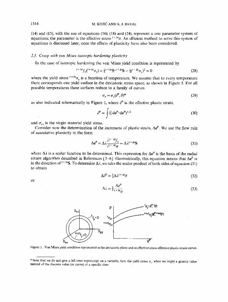
where the yield stress is a function of temperature. We assume that to every temperature there corresponds one yield surface in the deviatoric stress space, as shown in Figure 1. For all possible temperatures these surfaces reduce to a family of curves

py = d y ( ~ p , e)* (29) as also indicated schematically in Figure 1, where 2' is the effective plastic strain,

and rsyv is the virgin material yield stress.

of associativc plasticity in the form Consider now the determination of the increment of plastic strain, AeP. We use the flow rule

where A i is a scalar function to be determined. This expression for AeP is the basis of the radial return algorithm described in References 13-61. Geometrically, this equation means that AeP is in the direction of t + A f S . To determine Ai, we take the scalar product of both sides of equation (31) to obtain

fy=0 BYY SX, fy=0

t

Figure 1. Von Mises yield condition represented in the deviatoric plane and as effective stress-effective plastic strain curves

*Note that we do not give a left time superscript on a variable, here the yield stress oy, when we imply a generic value instead of the discrete value (or curve) at a specific time


'TY t

General Case Bilinear Curve

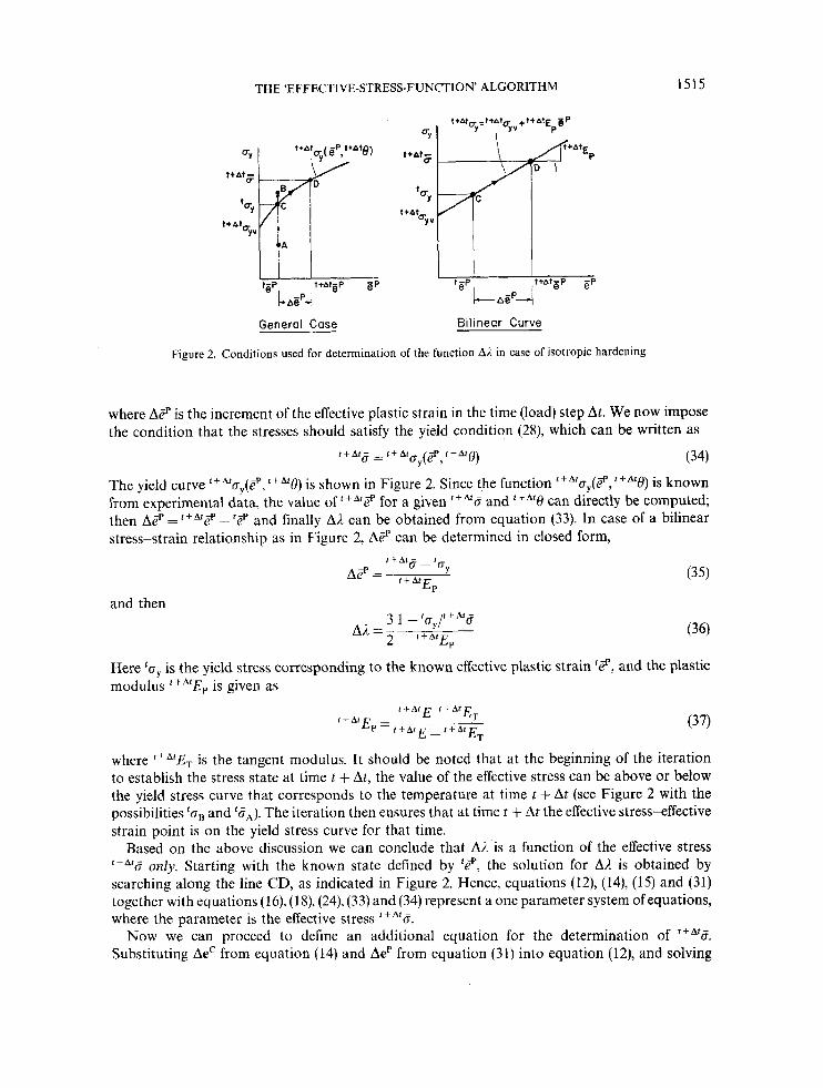
Figure 2. Conditions used for determination of the function A1 in case of isotropic hardening

where At? is the increment of the effective plastic strain in the time (load) step At. We now impose the condition that the stresses should satisfy the yield condition (28), which can be written as

Y (34) t + A t o = t + A l b (zP,t+Al())

The yield curve t + A t ~ y ( i ? , is shown in Figure 2. Since the function r + A ' ~ y ( Z p , r + A r O ) is known from experimental data, the value of r+ArZP for a given tiAr17 and '+"O can directly be computed;

-P - r+At-P then Ae - e -'d and finally A>" can be obtained from equation (33). In case of a bilinear stress-strain relationship as in Figure 2, A 2 can be determined in closed form,

and then

Here f ~ y is the yield stress corresponding to the known effective plastic strain 't?', and the plastic modulus t+ArEp is given as

where trA'ET is the tangent modulus. It should be noted that at the beginning of the iteration to establish the stress state at time 1 + At, the value of the effective stress can be above or below the yield stress curve that corresponds to the temperature at time t + At (see Figure 2 with the possibilities 'tfB and ' ~ 7 ~ ) . The iteration then ensures that at time t + At the effective stress-effective strain point is on the yield stress curve for that time.

Based on the above discussion we can conclude that A i is a function of the effective stress f + A r C only. Starting with the known state defined by 'ZP, the solution for BE. is obtained by searching along the line CD, as indicated in Figure 2. Hence, equations (12), (14), (15) and (31) together with equations (16), (18), (24), (33) and (34) represent a one parameter system of equations, where the parameter is the effective stress t1arc7.

Now we can proceed to define an additional equation for the determination of '+*'I7. Substituting AeC from equation (14) and AeP from equation (31) into equation (12), and solving

1516

for '+"S we obtain

M. KOJIC AND K . J. BATHE

1 f + A f a , + aAt'y + A1

S = rfAte'' - (1 - a)At'y'S] t + A t

where f + A f 1 + r + A ' V

f + A f E

Taking the scalar product of both sides in equation (38) we obtain

(401 f ( t + A t , j ) = a2 t + A f 5 2 + bry - C 2 r y 2 - d2 = 0

where a = + MAP7 + AA b = 3(1 - r)Atf+Are"-'S (41) c = ( 1 - a)At'C

d2 = t f + A t e f l . t + A t e II

The coefficients b,c and d are constants that depend only on the known values, independent of whereas the value of the coefficient 'a' varies with r+At6. The function f ( f + A * 5 ) defined by

equation (40) is the effeective-stress-function whose zero provides the solution for Namely at this solution the assumptions used to calculate the creep and plastic strain increments, equations (14) and (31), as well as the yield condition, equation (28), are satisfied.

To solve the non-linear equation (40), we employ a simple and stable bisection procedure with an acceleration scheme. Once r+At8 has been calculated, equations (38), (14) and (31) are used to evaluate r + A t S , Aec and AeP. The computational procedure is briefly summarized in Table I.

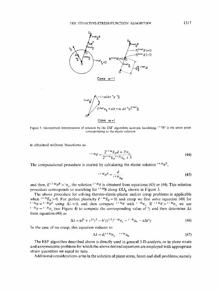
A geometrical interpretation of the computational procedure is presented in Figures 2 and 3. It should be noted that when x = 1 the direction of t+A'S is determined by the unit normal

where (42) '+Atn = f + A t R e / /I + *'err 11

j / t+Arer/ / / = ( r + A f e ! r . t + A t e " j 1 / 2

In the case of thermo-plasticity only ('y = 0), the effective stress function (40) reduces to

(43) f ( t + A f C j = ( f + A f a , + A ~ ) 2 I+A[62-d2=0

which is solved numerically using equations (33) and (34). When the yield curve is bilinear,

Table I. Solution steps in the effective-stress-function algorithm for thermo-plasticity and creep

1. Initialize value f + A r & ' ) = '5; then for k = 1,2,. . , 2. Compute ' y c r ) from the creep formula 3. Compute 4. Calculate the value of the effective stress function f('+A'b(k)) 5. Compute '+ A*&k + I ) . , here one step of a bisection algorithm

is used. If r+Af8(k+1) does not represent (to a specified tolerance) the solution, go to 2.

from the yield curve (when ' + > 'uy)

6. Compute '+*S, AeC, Aep and '


7 - t t A t S E

Case a - l

Figure 3. Geometrical interpretation of solution by the ESF algorithm; isotropic hardening; '+&SF is the stress point corresponding to thc elastic solution

is obtained without bisections as

f t A f - 2f+AfEpd + 3'0, O =

2t+AtEpf+AfuE + 3

The computational procedure is started by calculating the elastic solution r+4r8, ' + A t - E - d

(7 - t + A f a E

(44)

(45)

and then, if * '*'aE > 'cr,, the solution '+*'if is obtained from equations (43) or (44). This solution procedure corresponds to searching for t+A'S along DDE shown in Figure 3.

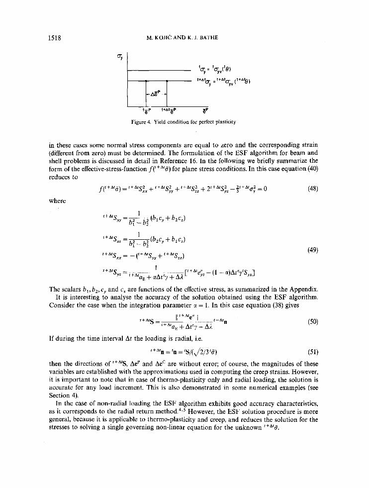
The above procedure for solving thermo-elastic-plastic and/or creep problems is applicable when ttAtEp > 0. For perfect plasticity = 0) and creep we first solve equation (40) for t + A l g = t + A t - E o l + A l - o =

using A i =0, and then compare '+*'if with l f A 1 c r y . If f 'ALif > ' t a f ~ y we use (see Figure 4) to compute the corresponding value of 'y and then determine A,?

from equation (40) as

aE - nAt'y (46) A I = (d2 + c 2 1 y 2 - b ~ ~ ) l ! 2 / r + A r ~ ~ - t + A t

In the case of no creep, this equation reduces to

UE AA = d / t + A f O y - (47)

The ESF algorithm described above is directly used in general 3-D analysis, or in plane strain and axisymmetric problems for which the above derived equations are employed with appropriate strain quantities set equal to zero.

Additional considerations arise in the solution of plane stress, beam and shell problems; namely


Figure 4. Yield condition for perfect plasticity

in these cases some normal stress components are equal to zero and the corresponding strain (different from zero) must be determined. The formulation of the ESF algorithm for beam and shell problems is discussed in detail in Reference 16. In the following we briefly summarize the form of the effective-stress-function f("Ar6) for plane stress conditions. In this case equation (40) reduces to

where

s, = - ? + A t s,, + + "'S,,) i + A t

['+ Ate;z - (1 - a)At'y 'S,,] I f + A t S =- ~~

f+AraE + ctAt'y + AI yz

(49)

The scalars b,, bZ,cy and c, are functions of the effective stress, as summarized in the Appendix. It is interesting to analyse the accuracy of the solution obtained using the ESF algorithm.

Consider the case when the integration parameter CI = 1. In this case equation (38) gives

If during the time interval At the loading is radial, i.e.

*+*'n = 'n = t S / ( J 2 / 3 t a ) (5 1)

then the directions of '+&St Aep and AeC are without error; of course, the magnitudes of these variables are established with the approximations used in computing the creep strains. However, it is important to note that in case of thermo-plasticity only and radial loading, the solution is accurate for any load increment. This is also demonstrated in some numerical examples (see Section 4).

In the case of non-radial loading the ESF algorithm exhibits good accuracy characteristics, as it corresponds to the radial return r n e t h ~ d . ~ . ~ However, the ESF solution procedure is more general, because it is applicable to thermo-plasticity and creep, and reduces the solution for the stresses to solving a single governing non-linear equation for the unknown t+At6.


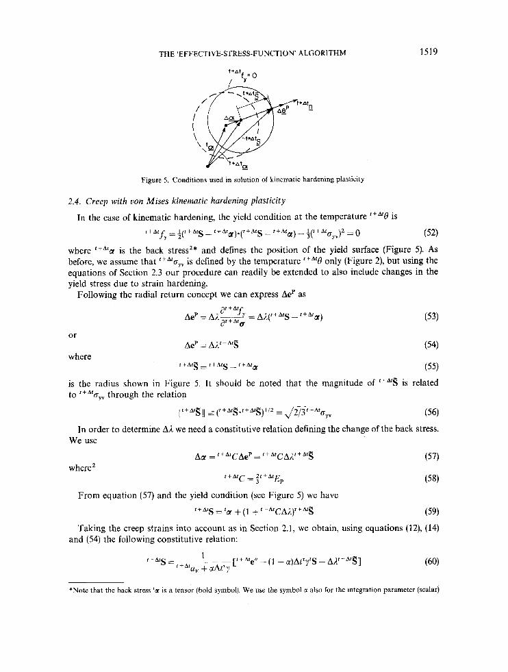
Figure 5. Conditions used in solution of kinematic hardening plasticity

2.4. Creep with uon Mises kinematic hardening plasticity

In the case of kinematic hardening, the yield condition at the temperature is f f A f f,=A 1 t + A f s - t + A t a ) . ( f + A r S - ' + A t a ) - +(t+AtG, , )2 = 0 (52)

where f f A r a is the back stress2* and defines the position of the yield surface (Figure 5). As before, we assume that t + A t ~ y v is defined by the temperature only (Figure 2), but using the equations of Section 2.3 our procedure can readily be extended to also include changes in the yield stress due to strain hardening.

Following the radial return concept we can express AeP as

or

where (54)

(55) is the radius shown in Figure 5. It should be noted that the magnitude of '+"S is related to f + A t nYy through the relation

l i t + A f S 1 1 ( f + A t S . t + A t S ) l / Z = @ t + A t G y v (56)

In order to determine AL we need a constitutive relation defining the change of the back stress. We use

where'

From equation (57) and the yield condition (see Figure 5) we have

(59) t + A t s = tdl + (1 + f +AfcAA)f + A f S

Taking the creep strains into account as in Section 2.1, we obtain, using equations (12), (14) and (54) the following constitutive relation:

*Note that the back stress 'a is a tensor (bold symbol). We use the symbol a also for the integration parameter (scalar)


From the last two equations the radius can be obtained as

where

1 s = ay i- (1 + ‘+AtCa,)Al

t + A t

a, = t+A‘aE + ixAt‘y

g = t+Ate“ - ay‘a - (1 - u)At‘y‘S (63) Now we can use the condition that the magnitude of is determined by equation (56) and

this gives A l . Taking the scalar product on both sides of equation (61) and solving for AA, we obtain

where I/ g I1 = (g.gP2 (65)

As in the case of isotropic hardening, A l is in equation (64) a function of the effective stress ‘ + A t i f , However, if creep strains are not included, A1 is independent of ‘+“if and is a constant determined by the strain ttAte” and the conditions at the start of the time step, which are considered to be known.

The effective-stress-function is formed by using equation (60). Taking scalar products on both sides of equation (60) we obtain

where

The computational procedure for kinematic hardening plasticity and creep is basically the same as when isotropic hardening is considered, see Table I. The difference is now in the computation of A i . Namely, A l is calculated from equation (64), and then to determine the value of f c+At8 ) , the radius is computed using equation (61).

Note that when there are no creep strains, the bisection algorithm is not employed: if the elastic solution gives stresses outside the yield surface, A l is computed using equation (64), is obtained from equation (61) and

We may note that in the case of no creep, our algorithm can be interpreted as the radial return mapping technique,’O with the appropriate change in the position of the yield surface. However, when creep is present, the displacement of the yield surface and the stress state do not correspond to the radial return method; this can be concluded from equations (60) and (61).

The above procedure for solving kinematic hardening (and creep) has been presented for general 3-D analysis (and plane strain and axisymmetric solutions for which simply the appropriate strains are set to zero). If plane stress or shell analyses are considered, modifications of the procedure presented here are necessary, see References 15 and 16.

Our observations about the solution accuracy in case of kinematic hardening are similar to those described for isotropic hardening. For example, if the loading is radial in a time (load) step, then in case of bilinear thermo-plasticity only, exact solutions are obtained for any integration time (load) step At. This is demonstrated in Section 4 (see Example 2).

is calculated using equation (59).

3. ELASTIC-PLASTIC-CREEP CONSTITUTIVE MATRIX

In this section we present a numerical procedure to compute the elastic-plastic-creep tangent constitutive matrix consistent with the ESF method. We want to compute a tangent constitutive

THE 'EFFECTWE-STRESS-FUNCTION' ALGORITHM 1521

matrix CEPC corresponding to the stress-strain state at the end of the time (load) step, which by definition is given by

, t + A t , * cEPcJ =___ r?* + *'e (68)

t + A l

To compute the above derivatives we use a perturbation procedure. Namely, we can write

where the column vectors are

C(') = 60("/6(') (no sum on i) (70)

and vector corresponding to 8') and n is the dimension of the constitutive matrix.

is the perturbation in the ith entry of the vector

The computational procedure consists of the following steps.

6d ' ) is the stress perturbation

1. Compute the vector t+Atc 2. From the perturbed strain vector

t+At- ( i ) = ' + A t e + &i) e where

S t ) = 6(')6, (no sum on i)

3. Compute the perturbed stress vector t-A'i?~i) and

O (73) h c ( ~ ) = t + A t # i ) - f f A t

4. Compute the column vector C") from equation (70).

The computation is performed using the ESF algorithm. At the start of the iteration for time step At we use an approximate CEPC matrix, since '+Are

has not yet been computed. Let t + A t S i be the ith component of the deviatoric stress vector and be a component of the deviatoric strain vector t+Afe', then we can obtain from equation (38) for isotropic hardening and/or creep, and from equations (60), (61) and (63) for kinematic hardening (and creep),

where for isotropic hardening,

and for kinematic hardening,

1 + + *'CA;t uy + ( 1 + f fArCuy)AA

c'=

The approximate sign in equation (74) indicates that changes in AA and ' y due to changes in are neglected. Also, it should be noted that CI = 1 is used in equations (75) and (76). From

*Note that we use here engineering strain variables

1522

equation (10) we obtain

&I. KOJIC AND K. J. BATHE

Using the definitions of urn and ‘+*‘Sij given in equations (9) and (lo), the expressions for the Cyc can be derived from equations (74) and (77). For example, in the case

l+Are!. . y,

of plane strain analysis, we obtain cEPC c E P C 0

11 12

c:y 0 C E P C

3 3 - Symm.

cEPC =

where

We have implemented this procedure in ADTNA and observed good convergence characteristics (see Example 4). Also, the cost of evaluating this tangent constitutive matrix is quite reasonable.

4. EXAMPLE SOLUTIONS

In this section we present a number of example solutions which demonstrate the effectiveness of the ESF algorithm. In the first three examples we study the accuracy of thermo-plasticity solutions when a 2-D element (plane stress or plane strain) is subjected to radial and non-radial loading conditions. The last example shows the stability, as well as the accuracy, obtained in a creep solution.

The solutions are obtained using the ADINA computer programI7 in which the ESF algorithm has been implemented.

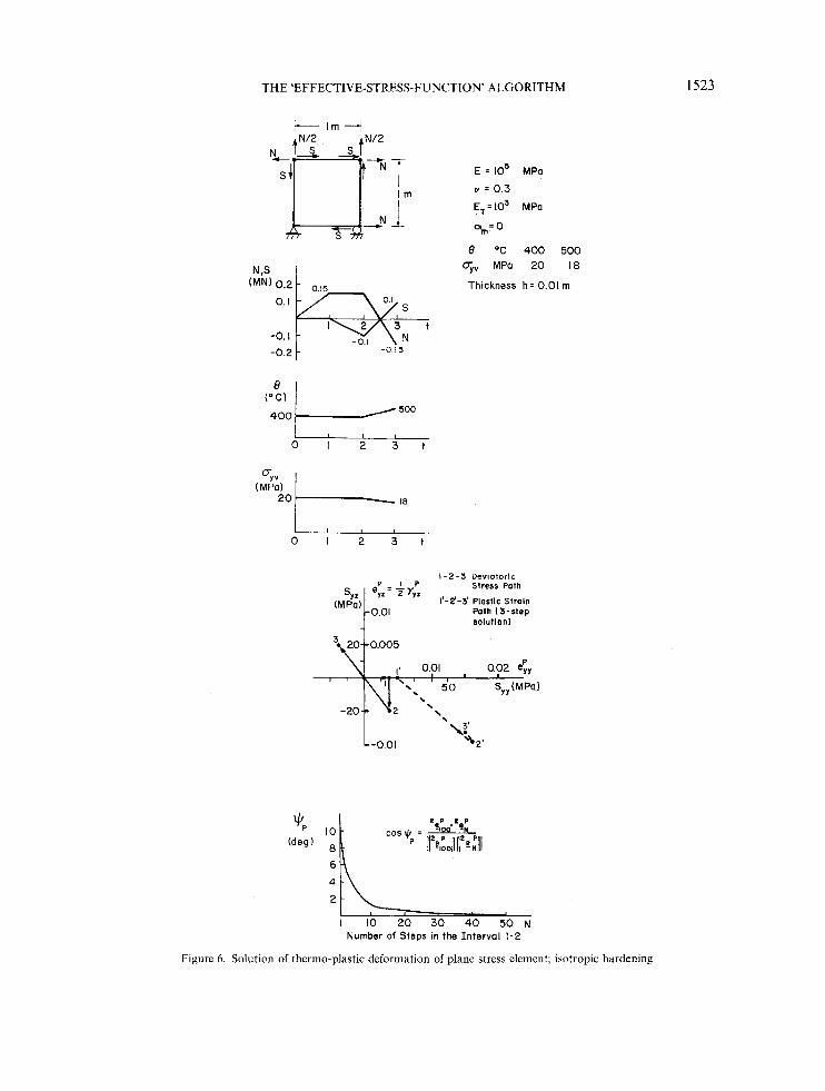
Example I. Thermo-plastic de$wmation of plane stress element (isotropic hardening)

The plane stress element shown in Figure 6 is subjected to biaxial tension and shear, according to the loading curves shown. The changes of temperature over time and the virgin yield stress as a function of temperature (and time) are also shown in the figure.

The loading in the time interval 0 to 1 is radial, in the interval 1 to 2 is non-radial, and from 2 to 3 we have reverse radial loading.

In the intervals 0 to 1 and 2 to 3, the solutions for increments of plastic strains are exact for any number of integration time steps. In the non-radial loading interval, the increments of plastic strains change direction and the solution depends on the number of time steps used in that interval. The 100-step solution in the non-radial loading interval is taken as the baseline solution, and the accuracy is studied by defining the angle $,. As shown, the accuracy of solution increases rapidly with the number of integration time steps used.

THE 'EFFECTIVE-STRESS-FUNCTION ALGORITHM

syz (MPa)

t-- 1 m - I

E = lo5 MPa

u . 0 3

€,=lo3 MPa

am= 0

8 OC 400 500 ayv MPa 20 18

Thickness h = 0 01 m 0. I

-0. I -0 2 -015

l'-2'-3' Plasllc Strain Path (3-s tep solution)

Y I 2 YYZ

-0.01

\

C' -0.01 y 2'

I 10 20 30 40 50 N Number of Steps in ?he In te rva l 1-2

Figure 6 . Solution of thermo-plastic deformation of plane stress element; isotropic hardening

1523


E = lo5 MPa v = 0.3 E,= lo’ MPa

a, = 0 + Thickness h = 0.01 m

OY Y

Y 8 OC 300 400 500

uyv MPa 14 12 10 i- i m - 4

%, -165.068

59.7290

I I I p

I 2 3 4 . t

IIIII I 2 3 4 t

I I I I

I 2 3 4 t

Interval Loading 0- I Radial

I - 2 Nonradial

2- 3 Radial

3 - 4 Reverse Radial

( MPa)

Positions of Yield Surface in Deviatoric Space

Error slpO0= Effective Plastic Strain

for N 100

Number of Steps in the Interval 1-2

Figure 7. Solution of thermo-plastic deformation of plane stress element; kinematic hardening

CTy 5 0 . (MPa)

5 E = 10 MPo v = o E,= 0

6 "C 20 500

uyv MPo 50 10

a = O

10

13 1-18.4783 (-26.3011 1

I n terva I Loading

0- I Elastic I - 2 Plastic -Nonrodiol 2 - 3 El. Plastic -

Reverse Radial

250-Anolyt icol es,.2SN Solution c o s + = J -

3 2 2 0 2 10

5k

Y '5,- Numerical

Solution; N steps u I 10 20 30 40 50 F\]


Error (Yo)


Figure 8. Solution of thermo-plastic deformation of plane strain element; perfect plasticity

1526 M. KOJlC AND K. J. BATHE

Creep Formula

ec F(I-dR')+Gt E = 21.71- 10' psi Y = 0.3 F = a, crag , R = a,eOsu

G = a4Csinh(a5u.)las SIDE VIEW

0.16111 a*= 1.608.16'0 a4=6.73.10-9

.c Y

al = 1.483 as= 1.479.104

02= 5.929.1d6 a,= 3.0

a3= 2.029.104

L

AXlSYMMETRlC MESH

Y

a) Finite Element Mesh and Material Data

I1000 r o a = O A t = 10 FOR 0 5 t S 1 0 0

t 7000 t

I I I 1 I

loo 10' loe lo3 10' 10' Time (hr)

b) Baseline Solution for the Effective Stress at Location A

Figure 9. Analysis of creep of thick-walled cylinder

THE 'EFFECTIVE-STRESS-FUNCTION ALGORITHM

0 a s 0 At =zoo - BASELINE SOLUTION

.- m n -'"t - \

0 I I I I I

loo 10' lo2 lo3 10' lo8 Time ( h r )

c) Effective Stress at Location A

UNSTABLE

b

a - 0 At * 500

-EASELINE SOLUTION

t

4000 t d) Effective Stress at Location A

Figure 9. (Continued)

1527


t o a ' 0 . 5 At = 6000

7000 1 - BASELINE SOLUTION

t 0

0

1 I I 1 I I

loo 10' lo2 lo3 lo4 105 Time (hr)

e) Effective Stress at Location A

01.1

I1000 r ~ t = 5.10' A A t * 5 . 1 O 4

- BASELlNE SOLUTION

.- ul

c Ln - ._ t 8000 - a)

W L. 'c -

7000 t 1 I I I I I

loo 10' lo2 lo3 lo4 105 Time ( h r )

f ) Effective Stress at Location A

Figure 9. (Continued)

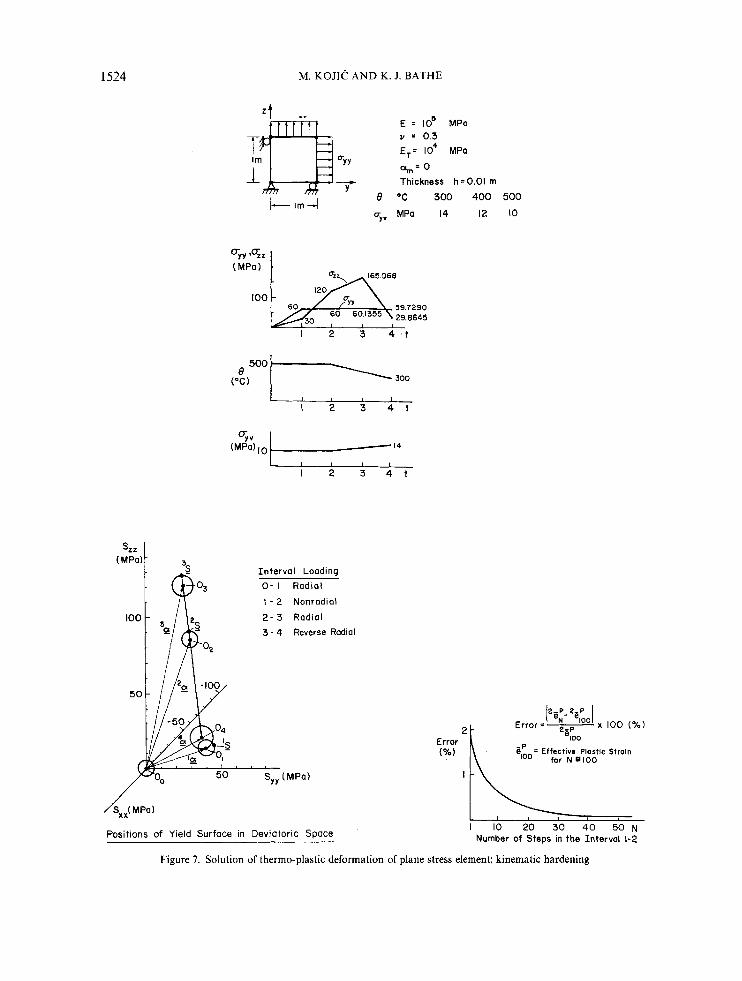
Example 2. Themo-plastic deformation of plane stress element (kinematic hardening)

The plane stress element shown in Figure 7 is subjected to radial, non-radial, and reverse radial loading conditions. As in the case of isotropic hardening, the solution is exact in the radial loading, even for large translations of the yield surface. The percentage error in the effective plastic strain at time 2, measured on the 100-step solution, shows a rapid decrease as the number of time steps is increased.


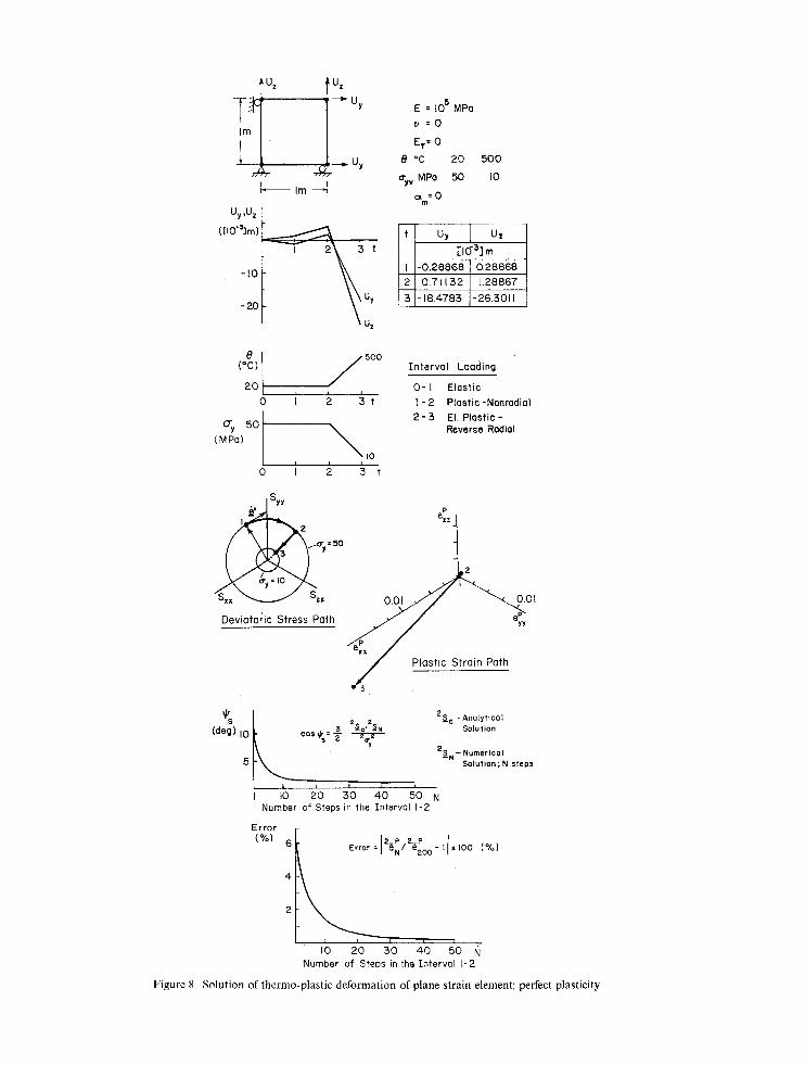
Example 3 . Thermo-plastic deformation of plane strain element (perfect plasticity)

The plane strain element of Figure 8 is subjected to biaxial straining. Once initial yield has been reached (at point 1 on the yield surface), the element is strained with constant strain rate such that the direction of the deviatoric strain rate e is in the tangential direction to the yield surface at point 1. In the time interval 0 to 2 oYv is assumed to be constant, in order to compare the numerical results with the analytical solution of Reference 4. The accuracy of solution is measured by the angle $s between the deviatoric stress vectors 'S, and ' S X , and also by the error in the effective plastic strain, 'e;, where N denotes the number of time steps used. The errors in the deviatoric stress and in the effective plastic strain decrease rapidly as the number of steps is increased.

In the radial loading interval 2 to 3, the solution is exact for any number of time steps, although there is a severe change in the yield stress.

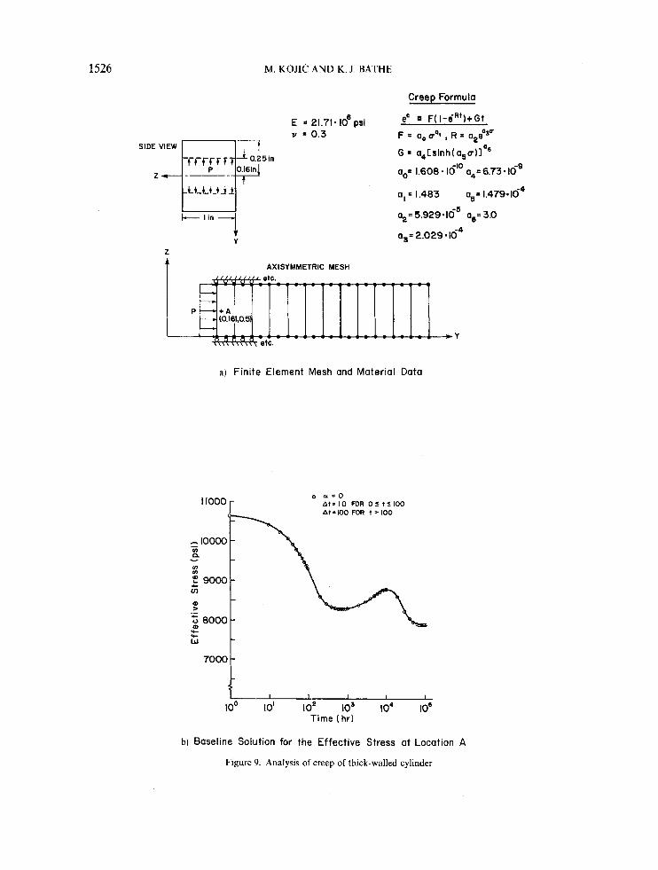
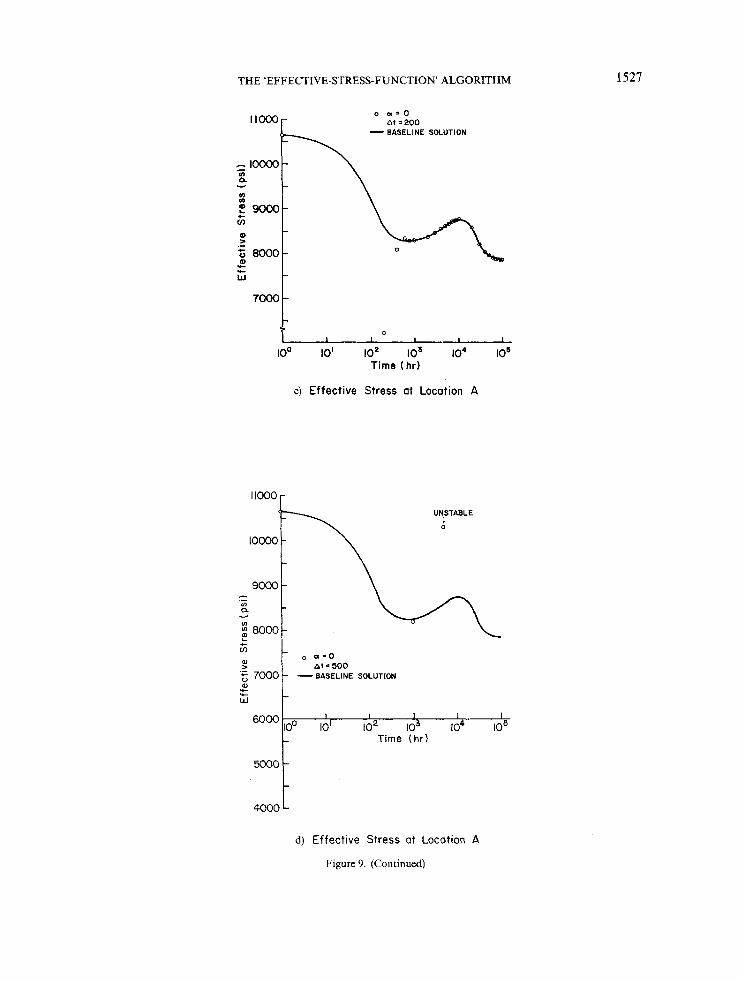
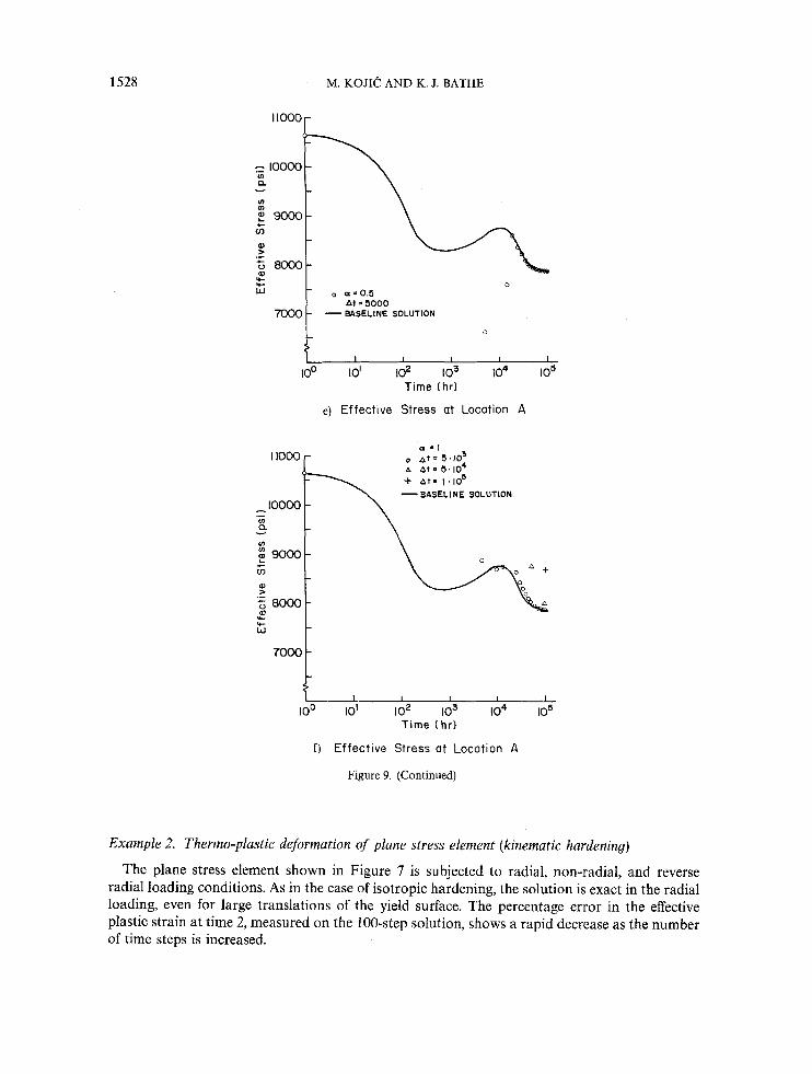
Example 4 . Creep of a thick-walled cylinder

In this example we demonstrate the accuracy of solution obtained when the ESF algorithm is applied to a creep problem, The results are compared with the solutions in References 2 and 12.

The problem considered and the finite element mesh used are shown in Figure 9(a). All solution results presented here are obtained by starting the creep solution from the initial elastic solution.

A baseline solution obtained with the ESF algorithm is shown in Figure 9(b). A comparison of this solution with the averaged solution results obtained with five computer programs" shows a difference of less than 2.3 per cent.12 Figures 9(c) to (f) show further solutions obtained with the ESF algorithm using different time steps and values of the integration parameter CI. As expected, the results are practically identical to those reported in Reference 2. Also, when a = 1, even with a time step of At = lo5 a reasonable solution is obtained using the ESF algorithm, the error being about 1 1 per cent!

To demonstrate the effectiveness of using the elastic-plastic-creep constitutive matrix derived in Section 3, we show in Table I1 some results regarding the equilibrium iterations. The results correspond to At = lo5 and the full Newton iteration method' with the use of our elastic-plastic- creep matrix.

The results in Table I1 show excellent convergence characteristics.

5. CONCLUSIONS

A procedure for the stress integration in thermo-elastic-plastic and creep analysis has been presented. The method-called the effective-stress-function (ESF) algorithm-falls into the

Table 11. Unbalanced energy and unbalanced force during equilibrium iterations (full Newton method with use of

elastic-plastic creep constitutive matrix)

0.82 x lo-'

0-13 x 10-15

0.4 x 104

0.53 x 10-4

0.90 x 10-4 0.82 x lo-*

0.39 x lo2 0.17 x 10'


category of radial return methods but is more general because it is applicable to thermo-elasto- plasticity and creep. Consistent with the ESF algorithm a tangent stress-strain relationship for the calculation of the element stiffness matrices has also been presented.

The main characteristics of the ESF algorithm are as follows. The method is computationally stable and accurate because the otherwise complex stress

integration in thermo-elasto-plasticity and creep is reduced to the solution of a single equation. This effective-stress-function equation is solved using a simple and robust bisection technique.

In thermo-elastic-plastic solutions, the algorithm exhibits excellent solution accuracy in radial loading, even for very large load steps, and in non-radial loading good accuracy is obtained when using reasonable load step magnitudes.

In creep analysis the method displays no difficulties in the solution of the implicit integration equations. Hence there is practically no restriction on the time step size At to converge in the stress solution. Of course, the accuracy of the creep solution depends on the magnitude of the time step used.

The method is directly applicable to large strain analysis." In this paper we considered only the analysis of problems modelled by the traditional von

Mises plasticity and pressure-independent creep laws. Here, the only variable in the computations of the inelastic strains is the effective stress. An extension of our approach to material laws in which the inelastic strains depend on more than one variable would require the formulation and solution of additional functional relationships involving these variables.

Our experiences with the ESF algorithm are most encouraging and we believe that the solution procedure provides an excellent basis for the development of more automatic and error-controlled schemes for inelastic finite element solutions.

APPENDIX

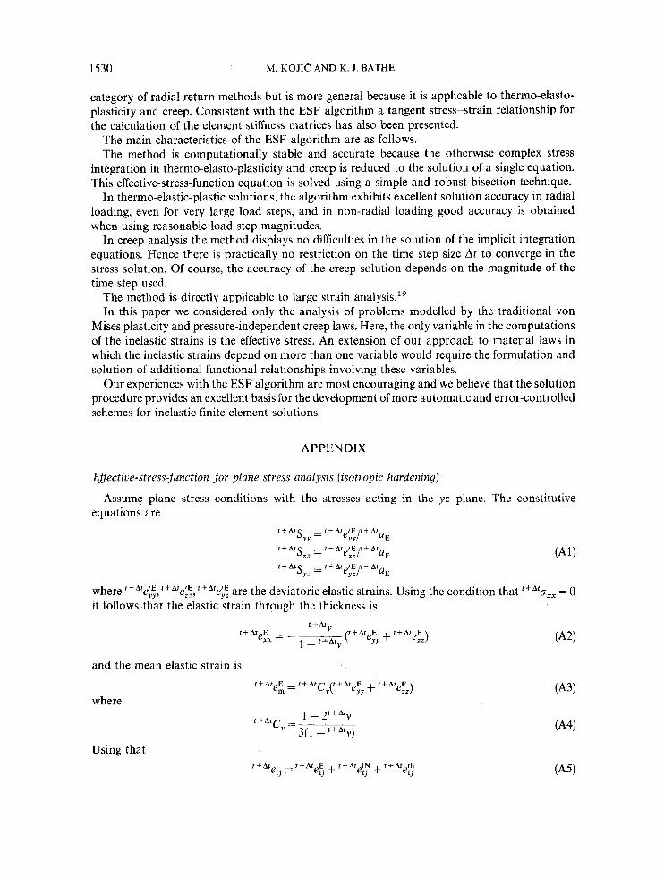
Eflectiue-stress-junction jor plane stress analysis (isotropic hardening)

equations are Assume plane stress conditions with the stresses acting in the y z plane. The constitutive

t + A t S = ? + A t r E / t + A t

f + A t f + A t I € t + A f YY C,YI a E

r + A t S,, = t+Ate"/t+AfaE s z z = ezz l aE

where t+Atej$ t + A r e : ~ , t + A t e ~ ~ are the deviatoric elastic strains. Using the condition that t+Araxx = 0 it follows that the elastic strain through the thickness is

and the mean elastic strain is

where

Using that

?+Ate,, = t + A t C y ( t + A f E eYy + +

THE 'EFFECTIVE-STRESS-FUNCTION' ALGORITHM 1531

where the ""'e!," are the inelastic strains,

(A6)

(A7)

1 + AtelN = t + At P LJ e,, + + "e;

and the t+Ate:," are the thermal strains, we can obtain from equations (A3) and (A5) t+AteIN - r + A t IN -

t + A t E - t + A f e,, 2'+A'e'h) em - C,, ( f+Atey , , + - Yl

N~~ t + A f rE e,,, and can be expressed as [ + A t ,E - f + A f I ?

t + A f rE - r + A t ezz ( I - (1 - ' + A t C , ) A e ~ ~ + *+"'CvAe; (AS) eY1 -

ezz -

e,,, - ( 1 - f+ArC,)AeE + "A'C,Aei~

where t + A t eYs II - - (1 - t + A t ~ ~ ) t + A f ~ ~ ~ - r + A t ~ ~ t + A t ~ ~ ~ - (1 - A ArCY)teE

+ Ateth + t + A t C v t e I N - (1 - 2 t + A Z zz

[ + AfCvf +AteYY - (1 - t+AtCv)fei: + t + A t C y t e T N YY - ( I - 2 t + A t c V ) r + A f e t h

f + Ate"z = ( 1 - f + A t C v ) t + Ate,, -

('49) Substituting equation (A8) into equation (Al) we obtain

t + A t u E t + A r S

t + A t u E r + A t S

= t+Ate:Y - (1 - t + A t c , ) A e E + t+Afc,~,,,; = ( + A t ezz R - (1 - r+AtCY)Ae~: + frAtC,,Ae:~ (A101 Y Y

Z Z

Next we use equations (14) and ( 3 1) to express Aei: and Ae::. Then, solving from equation (A10) for f+AtSYy and t+AfSzz we obtain

f + A t S V ) , = (b,c, + b,c,)/(b: - &;) (Al l ) *+AtSZZ = (b,c, + &,c,)/(b: - b;)

where h, = t + A t ~ E + (1 - f+AtC, ) (A2 + aAt'y) b, = t+A'C,(AI, + aAt'y)

(A 12) c y = t + A f evJ,-(t I I - ~ ) [ ( l -t+AfC,)'Syy-'+AfC,'Sz,]Aht'y c z = f + A l ezr 1' - ( 1 -.)[(I -t+AfC,l)tSZz - t+A*CvtSyy]At'y

The quantities b,, b,, cy and c, depend on the effective stress t + A t ~ . As before, the deviatoric stress t + A f S y z is expressed in terms of by equation (38). Then the effective-stress-function has the form (48).

strain through the thickness r+Afexx can be obtained as Finally, once and t + A l ezz IN have been computed after solving equation (48), the total

where

(A14) t + A f IN r + A t IN t + A l IN exx = - ( e y y + e z z )

REFERENCES 1. K. J. Bathe, Finite Element Procedures in Engineering Analysis, Prentice-Hall, Englewood Cliffs. N.J., 1982. 2. M. D. Snyder and K. J. Bathe, 'A solution procedure for thermo-elastic-plastic and creep problems', J . Nucl. Eng.

3. A. Mendelson, Plasticity, Theory and A p p l m t i o n , Robert E. Krieger Pub. Co., Malabar, Fla.. 1983. Des., 64, 49-80 (1981).

1532 M. KOJlC AND K. J. BATHE

4. R. D. Krieg and D. B. Krieg, ‘Accuracies of numerical solution methods in the elastic-perfectly plastic model’, ASME J . Press. Vess. Tech., 99, 510-515 (1977).

5. H. L. Schreyer, R. F. Kulak and J. M. Kramer, ‘Accurate numerical solutions for elastic-plastic models’, ASME J . Press Vess. Tech., 101, 226-234 (1979).

6. J. C. Nagtegaal, ‘On the implementation of inelastic constitutive equations with special reference to large deformation problems’, Comp. Methods Appl. Mech. Eng., 33,469-484 (1982).

7. S. W. Key and R. D. Krieg, ‘On the numerical implementation of inelastic time dependent and time independent, finite strain constitutive equations in structural mechanics’, Comp. Methods Appl. Mech. Eng., 33, 439-52 (1982).

8. M. Ortiz, P. M. Pinsky and R. L. Taylor, ’Operator split methods for the numerical solution of the elastoplastic dynamic problem’, Comp. Methods Appl. Mech. Eng., 39, 137-157 (1983).

9. J. C. Simo and R. L. Taylor, ‘Consistent tangent operators for rate-independent elasto-plasticity’, Comp. Methods Appl. Mech. Eng., 48, 101-118 (1985).

10. M. Ortiz and J. C. Simo, ‘An analysis of a new class of integration algorithms for elastoplastic constitutive relations’, Int. j . numer. methods eng., 23, 353-366 (1986).

11. R. K. Penny and D. L. Marriott, Design for Creep, McGraw-Hill, London, 1971. 12. M. D. Snyder and K. J. Bathe, ‘Finite element analysis of thermo-elastic-plastic and creep response’, Report No.

13. C. E. Pugh, et al., ‘Currently recommended constitutive equations for inelastic design analysis of FFTF components’,

14. C. E. Pugh, el al., ‘Interim guidelines for detailed inelastic analysis of high temperature reactor system components’,

15. M. KojiC and K. J. Bathe, ‘Solution procedures for inelastic structural analysis’, Report, ADINA R & D, Inc.,

16. M. Kojii: and K. J. Bathe, ‘Thermo-elasto-plastic and creep analysis of shell structures’, Comp. Struct., in press. 17. K. J. Bathe, ‘Finite elements in CAD and ADINA’, A’ucl. Eng. Des., 98, 57-67 (1986). 18. J. A. Clinard, et al., ‘Verification by comparison of independent computer program solutions’, in D. E. Dietrich (ed.),

Pressure Vessels and Piping Computer Program Evaluation and Qualification, PVP-PB-024, A.S.M.E., New York,

19. K. J. Bathe, R. Slavkovii: and M. KojiC, ‘On large strain elasto-plastic and creep analysis’, in P. G. Bergan et al.

82448-1 0, Acoustics and Vibration Laboratory, Department of Mechanical Engineering, MIT, 1980.

Report No. TM-3602, Oak Ridge National Laboratory, Oak Ridge, Tenn., 1972.

Report No. ORNL-5014, Oak Ridge National Laboratory, Oak Ridge, Tenn., 1974.

Watertown, MA, U.S.A., 1987.

1977, pp. 27-49.

(eds), Finite Element Methods for Nonlinear Problems, Springer-Verlag, Berlin, 1986.

The `effective-stress-function' algorithm for thermo...

Documents

Transcript of The `effective-stress-function' algorithm for thermo...