THE EFFECT OF METRO RAIL ON AIR POLLUTION IN DELHI Effect of Metro... · THE EFFECT OF METRO RAIL...

CDE April 2013

THE EFFECT OF METRO RAIL ON AIR POLLUTION IN DELHI

Deepti Goel

Email:[email protected] Department of Economics Delhi School of Economics

Sonam Gupta Email: [email protected]

Food and Resource Economics Department University of Florida, P.O. Box 110240 IFAS

Gainesville, FL32611, U.S.A.

Working Paper No. 229

Centre for Development Economics Department of Economics, Delhi School of Economics

The Effect of Metro Rail on Air Pollution in Delhi

Deepti Goel and Sonam Gupta

Abstract

In this paper we investigate the effect of the Delhi Metro, an intra-city mass rail transit system, on air

pollution within Delhi. To identify effects on pollution, we exploit the discontinuous jumps in metro

ridership, each time the network is extended. Our identifying assumption is that in the absence of the

extension there would be a smooth transition in pollution levels. We find strong evidence to show that

the Delhi Metro has resulted in reductions of two important vehicular emissions, namely, nitrogen

dioxide and carbon monoxide. We estimate a cumulative impact of a 35 percent reduction in CO

levels for the region around ITO (a major traffic intersection in Delhi). This is suggestive of a traffic

diversion effect, where people are switching from private modes of travel to the Delhi Metro. Given,

documented evidence on the adverse health effects of air pollution, our findings suggest that these

indirect benefits must be considered in any cost-benefit analysis of a rapid mass transport system.

The Effect of Metro Rail on Air Pollution in Delhi

Deepti Goel∗and Sonam Gupta†

1 Introduction

The Delhi Metro (DM) is an intra-city electric rail system serving the National Capital Region

(NCR) of India.1 Here we examine whether operation of this mode of public transportation,

first introduced in 2002, has had an impact on air quality in Delhi.

The motivation for this study comes from existing evidence on the adverse health effects

of air pollution. Block et al. (2012) define air pollution as a complex mixture that includes

carbon monoxide, sulfur oxides, nitrogen oxides, particulate matter (PM), ozone, methane

and other gases, volatile organic compounds (e.g., benzene, toluene, and xylene), and metals

(e.g., lead, manganese, vanadium, iron). They provide an excellent review of the state of

epidemiological research on the health effects of air pollution and cite several studies that link

damage of the central nervous system to air pollution, leading to decreased cognitive function,

low test scores in children, increased risk of autism and neurodegenerative diseases such as

Parkinson’s and Alzheimer’s. They also document research that shows that air pollution

causes cardiovascular disease (Brook et al., 2010) and can worsen asthma (Auerbach and

Hernandez, 2012). Turning to recent research in economics, Currie and Walker (2011) identify

the health effects of exposure to motor vehicle emissions using the introduction of electronic

toll collection and the consequent drop in emission levels in the vicinity of the toll sites.

They conclude that exposure to motor vehicle emissions increases the likelihood of pre-mature

births, and also causes low birth weight. Moretti and Neidell (2011) use daily boat traffic in the

∗Department of Economics, Delhi School of Economics, Delhi 110007, India; email: [email protected]†Food and Resource Economics Department, University of Florida, P.O. Box 110240 IFAS, Gainesville, FL

32611, U.S.A.; email: [email protected] NCR covers an area of about 33,578 sq kms. It comprises of the National Capital Territory of Delhi

at it core, nine districts in Haryana, five in Uttar Pradesh, and one in Rajasthan. At present, the DM servesDelhi, Gurgaon in Haryana, and Noida and Ghaziabad in Uttar Pradesh.

1

Los Angeles port as an instrument for ozone levels, and find that at least $44 million in annual

costs in Los Angeles are due to hospitalizations attributable to ozone related respiratory

ailments. Some other recent studies that examine the health consequences of air pollution

include Kenneth and Greenstone, 2003; Neidell, 2004; Currie and Neidell, 2005; Currie, Neidell

and Schmieder, 2009; and Lleras-Muney, 2010. Thus, there is substantiative evidence showing

that air pollution is harmful for human health.

Delhi has been documented to have high levels of air pollution. In its report on the ‘Na-

tional Ambient Air Quality status in 2008,’ the Central Pollution Control Board (CPCB) notes

that the city recorded critical levels of respiratory suspended particulate matter (RSPM/PM10).

Observed annual mean concentrations of RSPM were more than 1.5 times the acceptable stan-

dard for residential areas (CPCB, 2009). Using revised national ambient air quality standards

notified in 2009, the ‘State of the Environment Report for Delhi, 2010,’ documents that annual

average levels of RSPM exceeded the national standard (60 µg/m3) in the period between

1999 and 2008. This was also the case for nitrogen dioxide (national standard being 40

µg/m3) during the period from 2003 onwards, for recorded values till 2008. The report also

notes that carbon monoxide concentrations in ITO (a major traffic intersection in Delhi), ex-

ceeded the national standard (2000 µg/m3) between 1996 to 2008, though there is a declining

trend in recent years (DEF, 2010). Such high levels of pollution raise concerns for the health

of the city’s inhabitants.2 Studies by the CPCB find that high pollution levels in Delhi are

positively associated with lung function deficits and with respiratory ailments (CPCB, 2008a

and CPCB, 2008b). Guttikunda and Apte (2009) conduct a monitoring experiment in 2009,

and estimate that, every year, approximately 10,900 premature deaths in Delhi occur due to

ambient PM pollution.

In light of the above, it would be useful to study whether the DM has had any significant

impact on the city’s air pollution. Theoretical research from transport economics predicts

that the final impact on pollution could go in either direction (Vickery, 1969 and Mohring,

1972). The gist of the argument is that introduction of a new mode of public transport has two

2According to the latest Indian Census of 2011, the population of the Nation Capital Territory of Delhiis 16.8 million, with a density of 11,300 persons per square kilometer, making it one of the most denselypopulated regions of the world.

2

potential effects: traffic creation and traffic diversion. Improvement in the means of intra-city

transportation could lead to an increase in economic activity, and this could in turn generate

new demand for intra-city trips. It could also lead to residential relocation, away from the city

center to adjoining suburbs, resulting in longer commute distances to work. This is the traffic

creation effect, which presumably would increase pollution. On the other hand, commuters

who earlier relied on private means of transport may now switch to the new mode.3 This

traffic diversion effect would reduce pollution. Besides these two effects, one would also need

to take into account any pollution arising from the generation of electricity used to run the

DM. The DM draws electricity from three sources, namely, the Northern Grid, Indraprastha

Gas Turbine Plant and the Main Line Railway. Some of this maybe generated in coal based

power plants located within the city. Thus, the sign and magnitude of the net impact needs

to be determined empirically.

This paper seeks to quantify the causal effect of operation of the DM on air pollution using

secondary data from several sources, including hourly levels of ‘criteria’ pollutants. ‘Criteria

air pollutants’ is a term used to describe air pollutants that are being regulated within a

country and are used as indicators of air quality. The standards used to regulate the levels

of these pollutants are based on criteria that relate to health and/or environmental effects of

each pollutant. The criteria pollutants that we consider here are, nitrogen dioxide (NO2),

carbon monoxide (CO), ozone (O3) and sulphur dioxide (SO2).

To be able to attribute changes in pollutant measures to the DM, we need to address

concerns about endogeneity. An Ordinary Least Squares (OLS) regression of a pollutant

measure on metro ridership over time does not take care of endogeneity. This is because, typ-

ically, the intensity of utilization of different modes of transportation are positively correlated:

periods of relatively high ridership on the metro coincide with periods of high automobile us-

age. Furthermore, pollution levels also tend to be higher during periods of high demand for

transportation. Consequently, OLS estimates would be biased upwards. We use regression

discontinuity to overcome endogeneity (Lee and Lemieux, 2010). We exploit the sharp dis-

continuities in metro ridership resulting from each extension of the rail network, and examine

3According to a report by the Delhi Metro Rail Corporation (DMRC, 2008), the DM has already takenthe share of 40,000 vehicles.

3

whether they coincide with corresponding discontinuities in pollutant measures. The iden-

tifying assumption is that, in the absence of the extension there would have been a smooth

transition in air quality over time. This assumption would breakdown if other events, that

also have a discontinuous effect on air quality, happen simultaneously. For example, if a city

wide strike is called on the same day as the extension of the metro line, we would not be able

to disentangle the two effects. To address this issue, we study the chronology of events in the

city and do not find any such occurrences.

Our identification strategy is similar to that used by Chen and Whalley (2012). They

look at the effect of the introduction of the Taipei Metro on air quality. While they use the

discontinuity arising from the opening of the metro system, we exploit the discontinuities

arising from each extension of the network. We cannot use the first opening of the metro line

for two reasons. First, we do not have high frequency pollution data that dates back to the

period when the metro was introduced. Second, even if we did have this data, it would be

incorrect to use opening ridership discontinuity for Delhi, because there was an unprecedented

transitory jump in metro ridership when it was first introduced (DMRC, 2008).4 By using

discontinuities in ridership that occur several years after the metro first started, we believe

that to a large extent we avoid capturing effects arising from one time joy rides and the

impact that we measure is the steady state effect. In addition, an additional benefit of using

discontinuities at each extension allows us to get at a range of estimates. In implementing the

estimations, we are constrained by a large number of missing observations for hourly pollution

data. The details of how we deal with this are explained in the empirical strategy section

below.

From our analysis we find evidence to conclude that the DM has led to a reduction in NO2

and CO levels for Delhi. Looking at each extension of the rail network as a separate event, we

find that it results in a 3 to 47 percent reduction in NO2 concentration, and a 31 to 100 percent

reduction in CO concentration. The estimates vary depending on the particular extension

and monitoring station being considered. Evidence using multiple extensions, suggests a

4On the first day itself, about 1.2 million people turned up to experience this modern transport system.As the initial section was designed to handle only 0.2 million commuters, long queues of the eager commuterswishing a ride formed at all the six stations . . . Delhi Metro was forced to issue a public appeal in thenewspapers asking commuters to defer joy rides as Metro would be there on a permanent basis (DMRC, 2008).

4

cumulative impact of a 35 percent reduction in CO levels for the region around ITO (a major

traffic intersection in Delhi). Both NO2 and CO are important constituents of vehicular

emissions and our findings are suggestive of the traffic diversion effect of the DM. Guttikundu

(2010) presents probable scenarios of shifts in traffic patterns in Delhi due to the DM. Based

on these, he estimates vehicular emission reductions that range from 20 to 54 percent. Our

identification relies on observed changes in metro ridership, and we consider overall changes

in criteria pollutants and not just changes in vehicular emissions. This might be a reason why

our estimates differ from his.

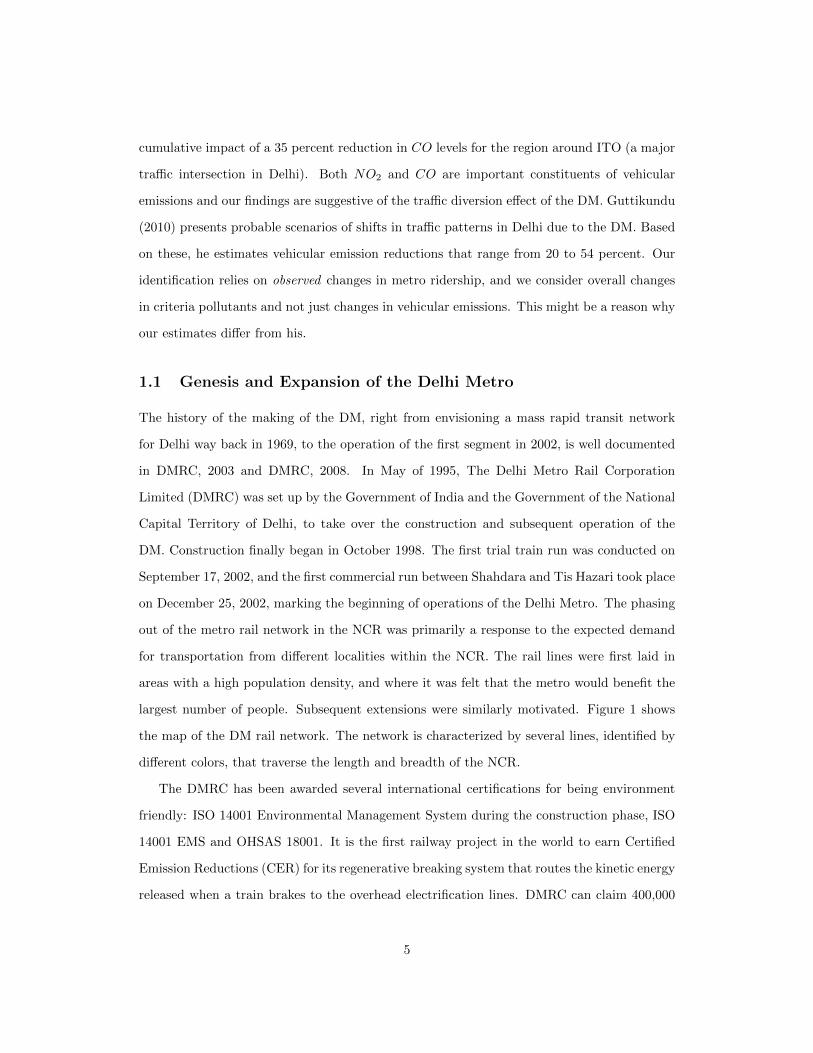
1.1 Genesis and Expansion of the Delhi Metro

The history of the making of the DM, right from envisioning a mass rapid transit network

for Delhi way back in 1969, to the operation of the first segment in 2002, is well documented

in DMRC, 2003 and DMRC, 2008. In May of 1995, The Delhi Metro Rail Corporation

Limited (DMRC) was set up by the Government of India and the Government of the National

Capital Territory of Delhi, to take over the construction and subsequent operation of the

DM. Construction finally began in October 1998. The first trial train run was conducted on

September 17, 2002, and the first commercial run between Shahdara and Tis Hazari took place

on December 25, 2002, marking the beginning of operations of the Delhi Metro. The phasing

out of the metro rail network in the NCR was primarily a response to the expected demand

for transportation from different localities within the NCR. The rail lines were first laid in

areas with a high population density, and where it was felt that the metro would benefit the

largest number of people. Subsequent extensions were similarly motivated. Figure 1 shows

the map of the DM rail network. The network is characterized by several lines, identified by

different colors, that traverse the length and breadth of the NCR.

The DMRC has been awarded several international certifications for being environment

friendly: ISO 14001 Environmental Management System during the construction phase, ISO

14001 EMS and OHSAS 18001. It is the first railway project in the world to earn Certified

Emission Reductions (CER) for its regenerative breaking system that routes the kinetic energy

released when a train brakes to the overhead electrification lines. DMRC can claim 400,000

5

CERs for a ten year crediting period beginning December 2007, translating to a gain of Rs.

1.2 crore per year (DMRC, 2008).

2 Empirical Strategy

We identify the effect of DM using Regression Discontinuity (RD) framework. Due to avail-

ability of data, we restrict our study period to 2004 − 2006. Table 1 shows the phase wise

extension of the metro network in this period. As shown, the DM rail network was extended

six times during this time. These extensions identify the potential discontinuities in metro

ridership and are the basis of our RD estimation. For each extension listed in Table 1, we

estimate the following equation:

yt = θ0 + θ1DMt + θ′

2xt + θ3P(t) + ut (1)

Here, yt is hourly pollutant level in logs at time t. yt could either be the level of the

pollutant at one of the three monitoring stations, or it could be the average of levels at two or

more stations. DMt is the discontinuity dummy characterized by each extension. It takes the

value one for all periods after an extension, and it is zero for periods before that.5 t extends

for an equal length of time on either side of the extension (typically, a one month on either

side, making it a 60 day window). Also, the equation is estimated only if there are no other

extensions within the length of time being considered. The vector of covariates, xt, includes

current and 1-hour lags of quartics of humidity, rainfall, temperature, and wind speed. In

addition, xt includes controls for hour of the day, day of the week (weekend or working day),

and interactions between hour and day of the week. P(t) stands for the third-order polynomial

in time. It controls for the smooth variation in pollutant levels in the absence of the metro

extension.6 θ1 is the coefficient of interest. It measures the percentage change in pollutant

5We exclude the 24 hour data on the day of the extension because we do not know the exact hour that thenew line became operational.

6Air quality can also be affected by government regulations aimed at reducing pollution. To the best ofour knowledge we do not know of any regulation that was implemented during our study period (2004−2006)and that would have a discontinuous effect on pollution. The mass conversion of diesel buses to compressednatural gas (CNG) happened earlier in 2001.

6

level due to the particular extension of the DM.

As mentioned in the introduction, our assumption is that within the period of estimation,

pollutant levels would have changed smoothly in the absence of the DM extension. After

controlling for weather and any other non-linearities using the polynomial time trend, any

observed change in pollutant levels around the extension may be attributed to the extension

itself.

One of our main challenges in estimating equation 1, is the lack of good quality hourly data

on pollutants. Our estimation strategy is severely constrained by the presence of contiguous

segments of missing observations in the pollution series. We restrict our analysis to only those

extensions for which there is at least a one month period on either side of the extension, in

which missing observations do not exceed 20 percent of maximum potential observations for

that month.7 We treat each metro extension as a separate event and analyze the metro effect

on each pollutant in its unique continuous time window. We start the analysis using a 60

day window around the extension, and later, we conduct robustness checks by extending the

window length wherever the data permits us to do so. As before, in determining the longer

window lengths as well, we extend the window by a month only if at least 80 percent of the

maximum potential observations are non missing. We intend to check the robustness of our

results by increasing this cut-off from 80 percent to 90 and 95 percent.

Missing data constrains us to study only five out of six extensions defined in Table 1. The

second extension of the red line is therefore excluded from our analysis. Table 2 summarizes

the extensions and the corresponding window lengths that we can consider, given the patterns

of missing pollution data. For instance, for ITO, we can examine the effect of opening of the

yellow line on only two pollutants (CO, SO2) out of four. Here, data allow us to extend the

60 day (2 months) window to a maximum of 180 days (6 months) for CO, and 300 days (10

months) for SO2. Table 2 shows that ITO has the best data with least missing observations.

Table 2 shows that for ITO, we have a fairly long series of good quality (in terms of missing

observations) data spanning from September 2004 to October 2005 for CO, and from October

2004 to March 2006 for SO2. We use this longer series to study the cumulative effect of DM

7The maximum potential hourly observations for a month is 720 (=24*30).

7

using the following equation:.

yt = δ0 + δ′

1xt + δ2P(t) +

K∑i=3

δi(DMi)t + εt (2)

The variables and coefficients are similarly defined as in equation 1. However, now the

time period extends over the longest possible contiguous segment of reasonably good quality

data, and accordingly includes K contiguous extensions. The cumulative effect of the DM

would then be given by∑K

i=3 δi.

Other specifications: We re-estimate equation 1 with 1, 2, 3, and 4 hour lags of outcome

pollutant. We have picked 4 lags after taking into account Henderson’s observation that

ozone persists in air for four hours in the US (Henderson, 1996). Inclusion of lags allows us to

examine the effect taking into account the persistence of pollutant concentrations in the air.

Our identification strategy relies on the crucial assumption that any discontinuous change

in air quality that is observed anytime a new segment of the network starts is due to the

particular extension. We include weather related variables in our models to capture changes

in weather conditions that might influence concentrations of pollutants in the air. Polynomial

time trend captures any smooth variation in pollution, demand for travel, and any other non-

linearities that might affect pollutant levels. Our identifying assumption could break down if

any unobservable factors lead to a discontinuous change in the air quality on the day of the

opening of Metro rail. One big threat to our empirical strategy could be the construction

activity undertaken to build Delhi Metro. One would expect this activity to slow down in

a continuous fashion just before the metro line becomes operational. Effect of this would

therefore we captured by the time polynomial. Second, our estimates might under- or over-

estimate the effect of opening of any of Delhi Metro lines if DMRC officials manipulated

the date of extensions. To us this seems highly unlikely. Given the enthusiasm of Delhi’s

inhabitants for the metro and the recognition of economies of scale in its operation, officials

were always in a hurry to open a new line.

8

3 Data and Descriptive Statistics

All our data comes from secondary sources. The National Data Center of the India Meteoro-

logical Department, provided hourly data for Delhi on four weather related variables, namely,

temperature, wind speed, rainfall, and relative humidity, for the period 2004 − 2006. The

Central Pollution Control Board (CPCB) of India collects air quality data for the National

Capital Territory (NCT) of Delhi as part of the National Air Quality Monitoring Program

(NAMP). The NAMP network consists of 342 monitoring stations all over the country, out of

which 11 stations are located in the NCT. Of these 11 stations, only 3 measure high frequency

hourly pollutant data. These are located at ITO (a traffic intersection in central Delhi), Siri

Fort (a residential area in south Delhi), and Delhi College of Engineering (DCE, in north Delhi

adjoining industrial areas). The criteria pollutants monitored by these stations are nitrogen

dioxide (NO2), carbon monoxide (CO), ozone (O3), sulphur dioxide (SO2), and two types

of particulate matter (PM10 and PM2.5).8 The CPCB provided us with this hourly data

for the time period 2004 − 2010. 9 Any analysis of pollution should control for atmospheric

conditions, and since we do not have weather data beyond 2006, we restrict our study period

to the years 2004 to 2006. At this stage, we focus on only four pollutants, namely, NO2, CO,

O3, and SO2. We omit particulate matter because data on it is very sparse. For our study

period, about 63 percent of all observations for PM10 and 43 percent for PM2.5 are missing.

Finally, line wise monthly ridership data was obtained from the Delhi Metro Rail Corporation

(DMRC).

Table 1 provides information about the phase wise extension of the metro network. It

shows that during the period 2004-2006, the red line was extended for the second time from

Inderlok to Rithala, yellow and blue lines were introduced and extended. The yellow line was

extended once, and the blue line was extended twice in this period.

Figure 2 and Figure 3 show the time series of monthly DM ridership and percentage change

in the DM monthly ridership for all lines in the time period 2004 − 2006. Both these graphs

show sharp discontinuities at red line extension 2, yellow line extension, blue line introduction,

8Only DCE provides data on PM10 and only ITO provides data on PM2.5.9Data from DCE starts from 2005.

9

and blue line extension 2.

Figures 3 to 7 display average monthly levels of concentrations of pollutants recorded at

each monitoring station, and average over the three monitoring stations. These graphs inform

us about a few distinctive features of the data. First, each monitoring station witnessed

different trends in concentrations of each pollutant. Compared to the other two stations, ITO

reported higher concentration of all pollutants, except O3. Second, one can observe that we do

not have complete time series for pollutant data for the entire study period. Hence, we cannot

average criteria pollutant data over all monitoring stations as done by Chen and Whalley

(2012). Although we do not have contiguous time series for the study period, figures show

clearly that we do have sufficient data to examine the effects of DM in shorter time windows.

We have exploited this fact in our empirical strategy. Third, we do observe a sharp change

in pollutant levels when the metro line is introduced/extended, although this is not seen for

all instances. In Tables 3 and 4, we report the descriptive statistics for the four pollutants

and weather related variables. In both the tables, first column shows the discontinuity being

studied.10 Second column reports the full sample mean, standard deviation, and sample size

for each discontinuity, followed by pre-discontinuity and post-discontinuity mean, standard

deviation, and sample size. Last column reports the difference between pre and post means

along with p-value (in parenthesis) of t-test that compares pre and post DM means of criteria

pollutants. These tables reveal a number of patterns. First, with few exceptions, levels of

concentrations of all the four pollutants are lower in the post-Metro period as compared

to the pre-Metro period. We also find that these differences are statistically significant in

most cases. Second, data from all three pollution monitoring stations shows that blue line

second extension from Barakhamba - Indraprastha led to statistically significant lower levels

of carbon monoxide post DM. Third, pollutant data from ITO and Siri Fort stations provides

consistent evidence that levels of concentration of SO2 and O3 were lower after the extension

of yellow line. Fourth, there are significant differences in all weather related variables in pre

and post DM values. Differences in weather related variables before and after the introduction

10We have only reported those discontinuities for each monitoring station that we examine in this paper.Both for weather related variables and pollutants we have only reported summary statistics calculated within60 day window.

10

or extension of almost all Metro lines, make it imperative that we control for atmospheric

conditions. Our empirical approach is discussed in detail in the previous section.

4 Results

Tables 5 to 7 report estimates from equation 1 for the effect of DM on criteria pollutant levels

around a 60 day window for each of the three monitoring stations. Each column displays

the estimates obtained by fitting equations for a particular pollutant, and each cell reports

the results from a separate regression. For each regression, we report the coefficient on the

discontinuity dummy, its standard error, and the number of observations (N).11

From these tables we make the following observations. First, data from ITO (Table 5) and

Siri Fort (Table 6) indicates that DM had a negative effect on levels of NO2. For ITO, each

extension of the metro network resulted in a decrease in NO2. The estimates range from 3.2

percent (yellow line extension) to 38.6 percent (introduction of the blue line). Except for the

first extension of the blue line, all estimates are statistically significant at the 1 percent level.

We observe the same pattern for Siri Fort, though the magnitude of reduction is higher. For

both the extensions for Siri Fort, we find about a 47 percent reduction in NO2 emissions.

Again, these estimates are statistically significant at the 1 percent level. For DCE, we find

positive coefficient values. However, in one case the estimate is marginally significant at the

10 percent level, and in the other it is not statistically significant at conventional levels.

Second, for both ITO and Siri Fort, we find that DM has reduced CO concentrations.

For ITO, the estimates range from 33 to 99.9 percent and for Siri Fort, it is 31.4 percent.

All estimates are significant at the 1 percent level. For DCE, we do not find statistically

significant results.

Third, we do not observe any consistent pattern across the three stations for SO2 emissions.

ITO shows significant increases, Siri Fort shows significant reductions, and for DCE the results

are insignificant. SO2 is mainly a non-transportation based pollutant and is an important

11In each regression, the sample size is determined by the number of non-missing observations for a particularpollutant, in the 60 day window around a particular extension (one of the six discontinuities listed in Table 1).Thus, sample sizes may differ across regressions. As stated earlier, we estimate a regression only if at least 80percent of the maximum possible observations (approximately 1440) are non-missing.

11

constituent of industrial emissions. It could be affected by localized activity such as the

location of coal based power plants within the city. This could be an explanation for lack of

consistent results across all monitoring stations.

Finally, for O3, our results are a bit puzzling at this stage as there is no consistent pattern

even when we look at estimates for each station separately (results for ITO in particular).

Ozone is a secondary pollutant formed in the atmosphere by reaction between oxides of

nitrogen and volatile organic compounds (VOCs) in the presence of sunlight. Peak O3 levels

generally occur during the summer when temperatures are higher. At this stage, our results

for O3 are perplexing and we need to investigate possible explanations for them.

Overall, we find evidence to conclude that the DM has led to a reduction in NO2 and CO.

Both these pollutants are an important constituents of vehicular emissions. This suggests that

one explanation for our results for these tailpipe emissions could be the traffic diversion effect

mentioned earlier. It is suggestive that the DM is encouraging more people to switch from

private to public means of transport.

We account for persistence of pollutants in the atmosphere by including up to 4 lags of

outcome pollutant as controls. Results for estimations with lagged pollutants are displayed

in Tables 8 to 10. As expected the magnitude of point estimates is much smaller in these

specifications as compared to the previous ones without lagged variables. The broad patterns

however, remain the same.

Next, we consider specifications longer than the 60 day window. Conceptually, it makes

sense to choose a shorter time period around the observed discontinuity. However, a longer

period gives more precise estimates due to increased sample size. The trade-off is that with a

longer window there is a greater possibility of having discontinuities arising from events other

than the metro extension. If such events do occur within the larger time span, then they would

distort our earlier results. In Tables 11 and 12 we report the results from re-estimating most

of the earlier regressions in with longer time series, and find that for NO2 and CO, whenever

the results were significant in the 60 day estimations, either the direction of the effect remains

the same (though magnitudes are smaller in the longer period estimations) or the estimate

loses significance.12 Ideally, increase in window length should only increase precision and not

12Window lengths differ for each regression depending on the pattern of missing observations for a particular

12

change magnitudes or signs of coefficients. These results require closer scrutiny. They may

be an indication of other discontinuities occurring within the longer window.

Table 13 reports results obtained after averaging hourly data across two or more moni-

toring stations. These regressions give us an estimate of effect of DM on overall pollution

levels for the city as a whole. These estimates show that DM improved overall air quality of

Delhi by reducing levels of NO2 by 22.7 percent and of CO by 23 percent. These results are

significant at 1percent level.

We use ITO data on CO from October 2004 to March 2006 to estimate the regressions

reported in Table 14, and ITO data on SO2 from September 2004 to October 2005 for Ta-

ble 15.13 The specification used is shown in equation 2 and is different from estimations

presented so far because we include multiple discontinuities. This enables us to estimate the

cumulative effect of the DM over time. Introduction of the yellow line resulted in a 22.2

percent decline in CO levels, followed by a further decline of 12.8 percent when that line was

extended. This is a cumulative effect of a 35 percent reduction in CO levels. The introduc-

tion and extension of the yellow line also led to a decline of 123.7 percent in SO2, though the

introduction of the blue line resulted in an increase of 29.3 percent. Thus, the cumulative

effect of the DM on SO2 is a decline of 94.4 percent.

We plan on conducting several robustness checks to test the validity of our estimates. We

intend to include details on industrial activity and traffic patterns in our analysis to help us

interpret the results better. Also, given that some of our results changed when we extended

the window length, we would like to re-estimate our regressions using a 30 day window, to see

if that makes a difference. Lastly, this paper could benefit by obtaining data from another

city to conduct a difference-in-difference analysis.

pollutant around the discontinuity being considered. Table 2 gives information on the exact window lengthused for each regression. As is seen from this table the longest window length is 10 months.

13Similar estimations for other monitoring stations and other criteria pollutants could not be carried outbecause a long continuous series of non-missing data for these was not available.

13

5 Summary and Conclusions

The Delhi Metro is an electric based public transit system serving the National Capital

Region of India. It was first introduced in Delhi in 2002. We quantify the effect of the DM

on air pollution in the city. We use hourly data on four criteria pollutants for the years 2004

through 2006. To identify causal effects, we use Regression Discontinuity framework. We

exploit jumps in metro ridership that are observed each time the rail network is extended,

and look for concomitant changes in pollutant levels. Controlling for weather conditions, hour

and weekday fixed effects, and a third order time polynomial, we attribute any discontinuous

change in pollutant levels around the extension date to the DM.

Our estimates show that each extension of the metro rail resulted in a decline in nitrogen

dioxide and carbon monoxide in Delhi. The estimates for nitrogen dioxide reductions range

from 3 to 47 percent, while those for carbon monoxide range from 31 to 100 percent. For ITO,

a major traffic intersection in Delhi, we find that the cumulative effect of multiple extensions,

is a net decline in carbon monoxide of 35 percent. Given that both nitrogen dioxide and carbon

monoxide are important tailpipe emissions, our findings suggest that the DM has encouraged

people to switch from private to public mode of travel resulting in positive externalities for

air quality in the city.

Given the huge health costs associated with high levels of air pollution, these indirect

health benefits should be taken into account when urban policy makers contemplate the

setting up large scale intra-city transportation systems. Our paper provides a rationale for

subsidizing these mass transit systems even when the direct accounting costs do not show a

net profit. The municipalities of many other tier I and tier II cities in India are planning to

build metro systems in their respective cities. Evidence of positive effect on air quality for

Delhi’s metro could provide a rationale for encouraging metro expansion in other cities that

face similar challenges in terms of vehicular congestion and health costs due to pollution.

14

References

Auerbach, Amya and Michelle L. Hernandez (2012) “The Effect of Environmental Oxidative

Stress on Airway Inflammation,” Current Opinion in Allergy and Clinical Immunology, 12

(2): 133-139.

Block, Michelle L., Alison Elder, Richard L. Auten, Staci D. Bilbo, Honglei Chen, et al.

(2012) “The outdoor air pollution and brain health workshop”, NeuroToxicology, forthcoming.

Brook, Robert D., Sanjay Rajagopalan, C. Arden Pope - III, Jeffrey R. Brook, Aruni Bhat-

nagar, Ana V. Diez-Roux, et al. (2010) “Particulate Matter Air Pollution and Cardiovascular

Disease : An Update to the Scientific Statement From the American Heart Association,”

Circulation, 121: 2331-2378.

Chay, Kenneth Y. and Michael Greenstone (2003) “The Impact of Air Pollution on Infant

Mortality: Evidence from Geographic Variation in Pollution Shocks Induced by a Recession,”

The Quarterly Journal of Economics, 118 (3): 1121-1167.

Chen, Yihsu and Alexander Whalley (2012) “Green Infrastructure: The Effects of Urban

Rail Transit on Air Quality,” American Economic Journal: Economic Policy, 4 (1): 58-97.

CPCB (2008a) “Epidemiological Study on Effect of Air Pollution on Human Health

(Adults) Delhi,” Environmental Health Series 1.

CPCB (2008b) “Study on Ambient Air Quality, Respiratory Symptoms and Lung Function

of Children in Delhi,” Environmental Health Series 2.

CPCB (2009) “National Ambient Air Quality Status 2008,” National Ambient Air Quality

Monitoring Series, NAAQMS/2/2009-10.

Currie, Janet, and Matthew Neidell (2005) “Air Pollution and Infant Health: What Can

We Learn from California’s Recent Experience?,” Quarterly Journal of Economics, 120 (3):

1003-1030.

Currie, Janet, Matthew Neidell, and Schmieder, Johannes F. (2009) “Air Pollution and

Infant Health: Lessons from New Jersey,” Journal of Health Economics, 28(3): 688-703.

Currie, Janet and Reed Walker (2011) “Traffic Congestion and Infant Health: Evidence

from E-ZPass,” American Economic Journal: Applied Economics, 3 (1): 65-90.

DEF (2010) “State of Environment Report for Delhi-2010,” Department of Environment

15

and Forests, Government of NCT of Delhi.

DMRC (2003) “A Dream Revisited: An Archival Journey into the making of the Delhi

Metro Rail,” Public Relations Department, Delhi Metro Rail Corporation Ltd, New Delhi,

India.

DMRC (2008) “A Journey to Remember,” Public Relations Department, Delhi Metro Rail

Corporation Ltd, New Delhi, India.

Guttikunda, Sarath (2010) “Estimated Air Pollution and Health Benefits of Metro System

in Delhi,” SIM-air Working Paper Series, 32.

Guttikunda, Sarath and Joshua Apte (2009) ”Monitoring & Mapping Urban Air Pollution:

A One Day Experiment in Delhi, India,” SIM-air Working Paper Series, 29.

Henderson, Vernon (1996) “Effects of Air Quality Regulation,” American Economic Re-

view, 86(4): 789-813.

Lee, David, and Thomas Lemieux (2019) “Regression Discontinuity Designs in Economics,”

Journal of Economic Literature, 48: 281-355. Lleras-Muney, Adriana (2010) “The Needs of

the Army: Using Compulsory Relocation in the Military to Estimate the Effect of Air Pollu-

tants on Children’s Health,” Journal of Human Resources, 45 (3): 549-590.

Mohring, Herbert (1972) “Optimization and Scale Economies in Urban Bus Transporta-

tion,” American Economic Review, 62 (4): 591-604.

Moretti, Enrico and Matthew J. Neidell (2011) “Pollution, Health, and Avoidance Behav-

ior: Evidence from the Ports of Los Angeles,” Journal of Human Resources, 46 (1): 154-175.

Neidell, Matthew J. (2004) “Air Pollution, Health, and Socio-Economic Status: The Effect

of Outdoor Air Quality on Childhood Asthma,” Journal of Health Economics, 23(6): 1209-

1236.

Vickery, William (1969) “Congestion Theory and Transport Investment,” American Eco-

nomic Review, 59(2): 251-60.

16

Table 1: Phase wise extension of the Delhi Metro during 2004-2006

Metro Line New Rail Segment Opening Date

Red Line Extension 2 Inderlok - Rithala 1 April 2004Yellow Line Introduction V ishwavidyalaya - Kashmere Gate 20 December 2004Yellow Line Extension 1 Kashmere Gate - Central Secretariat 3 July 2005Blue Line Introduction Barakhamba - Dwarka 31 December 2005Blue Line Extension 1 Dwarka - Dwarka Sector 9 1 April 2006Blue Line Extension 2 Barakhamba - Indraprastha 11 November 2006

Source: Delhi Metro Rail Corporation

17

Table 2: Discontinuities Studied During 2004-2006

Delhi Metro Rail Line NO2 CO SO2 O3

(Start Date)

Pollution Monitoring Station: ITOYellow Line Introduction

2-6 months 2-10 months(20th December 2004)Yellow Line Extension

2 months 2-10 months 2-10 months 2 months(3rd July 2005)Blue Line Introduction

2-4 months 2-4 months 2-4 months(31st December 2005)Blue Line Extension 1

2-4 months 2-4 months(1st April 2006)Blue Line Extension 2

2 months 2-4 months 2-4 months(11th November 2006)

Pollution Monitoring Station: Siri FortYellow Line Introduction

2 months 2-4 months 2-4 months(20th December 2004)Yellow Line Extension

2 months(3rd July 2005)Blue Line Extension 1

2 months(1st April 2006)Blue Line Extension 2

2-4 months 2-4 months 2-4 months(11th November 2006)

Pollution Monitoring Station: DCEBlue Line Extension 1

2 months 2 months 2 months 2 months(1st April 2006)Blue Line Extension 2

2 months 2 months 2 months 2 months(11th November 2006)

Mean Across Three Monitoring StationsBlue Line Extension 2

2 months 2 months(11th November 2006)

Mean Across Two Monitoring StationsITO + DCE

Blue Line Extension 12 months 2 months

(1st April 2006)Blue Line Extension 2

2 months(11th November 2006)

ITO + Siri FortYellow Line Introduction

2 months(20th December 2004)Yellow Line Extension

2 months(3rd July 2005)Blue Line Extension 2

2 months(11th November 2006)

18

Table 3: Summary Statistics for Criteria Pollutants During 2004-2006

Delhi Metro Rail Line Full Sample Pre Post Difference(Pre-Post)

Pollution Monitoring Station: ITO

Pollutant: Nitrogen DioxideYellow Line Extension 4.25 4.30 4.23 0.072*

(0.51) (0.48) (0.54) (0.099)N 1305 614 619Blue Line Introduction 5.29 5.40 5.18 0.220***

(0.61) (0.64) (0.57) (0.000)N 1399 679 720Blue Line Extension 1 4.85 4.82 4.87 -0.042

(0.49) (0.50) (0.48) (0.119)N 1302 616 686Blue Line Extension 2 4.99 5.00 4.99 0.005

(0.46) (0.50) (0.42) (0.844)N 1415 719 696

Pollutant: Carbon MonoxideYellow Line Introduction 7.37 7.49 7.25 0.241

(1.09) (1.25) (0.88) (0.000)N 1319 677 642Yellow Line Extension 7.39 7.45 7.32 0.130***

(0.72) (0.52) (0.87) (0.000)N 1344 653 691Blue Line Extension 2 7.92 8.05 7.78 0.269***

(0.63) (0.63) (0.61) (0.000)N 1415 719 696

Pollutant: Sulphur DioxideYellow Line Introduction 2.36 2.44 2.27 0.17***


(0.94) (1.10) (0.50) (0.000)N 1316 651 665Blue Line Introduction 2.98 2.50 3.43 -2.98***

(1.03) (0.98) (0.86) (0.000)N 1383 667 716

Pollutant: OzoneYellow Line Extension 2.60 2.77 2.42 0.07***

(1.25) (1.34) (1.11) (0.00)N 1233 645 588Blue Line Introduction 2.43 2.59 2.28 0.306***

(0.97) (0.76) (1.11) (0.000)N 1372 664 708Blue Line Extension 1 2.23 2.12 2.34 -0.219**

19


(0.79) (0.81) (0.73) (0.000)N 1407 713 694

Pollution Monitoring Station: Siri Fort

Pollutant: Nitrogen DioxideYellow Line Introduction 3.94 4.04 3.84 0.205***

(0.48) (0.48) (0.46) (0.000)N 1366 682 684Blue Line Extension 2 4.06 3.79 4.34 -0.556

(0.81) (0.48) (0.81) (0.000)N 1409 715 694

Pollutant: Carbon MonoxideBlue Line Extension 2 7.02 7.08 6.95 0.269**

(1.05) (1.08) (1.02) (0.029)N 1342 680 662

Pollutant: Sulphur DioxideYellow Line Introduction 1.17 1.13 1.23 -0.095


(0.51) (0.57) (0.42) (0.000)N 1225 598 627Blue Line Extension 1 1.68 1.56 1.81 -0.249***


(0.66) (0.74) (0.54) (0.000)N 1369 695 674

Pollutant: OzoneYellow Line Introduction 2.60 2.77 2.42 0.07***

(1.25) (1.34) (1.11) (0.00)N 1233 645 588

Pollution Monitoring Station: DCE

Pollutant: Nitrogen DioxideBlue Line Extension 1 3.32 3.36 3.27 0.090*


(1.37) (1.33) (0.71) (0.000)N 1369 693 676

Pollutant: Carbon MonoxideBlue Line Extension 1 7.24 7.27 7.23 0.043***

(0.27) (0.27) (0.28) (0.002)N 1411 718 693

20

Blue Line Extension 2 7.36 7.50 7.23 0.272***(0.43) (0.38) (0.44) (0.000)

N 1375 698 677Pollutant: Sulphur Dioxide

Blue Line Extension 1 1.99 1.17 2.85 -1.680***(1.79) (1.73) (1.42) (0.000)

N 1400 716 684Blue Line Extension 2 1.68 1.87 1.50 0.368***

(0.95) (0.87) (0.98) (0.000)N 1370 694 674

Pollutant: OzoneBlue Line Extension 1 5.46 5.35 5.58 -0.227***


(1.19) (1.17) (1.18) (0.000)N 1367 696 674Notes: In columns 2-4, in each cell the first entry is the mean of the log pollutant (measured in µg/m3), below

it in parenthesis is standard deviation, and the third entry is the number of observations. In the last column,

p-values are reported in the parenthesis. Each cell entry pertains to a 60 day window around the corresponding

extension. ∗∗∗, ∗∗, ∗ show statistical significance at the 1%, 5% and 10% levels respectively.

21

Table 4: Summary Statistics for Weather Related Variables

Delhi Metro Rail Line Full Sample Pre Post Difference(Pre-Post)

Relative Humidity (%)Yellow Line Introduction 72.17 72.47 71.87 0.609

(17.86) (18.10) (17.64) (0.5217)N 1416 696 720Yellow Line Extension 63.85 49.68 77.53 -27.85***

(21.75) (20.73) (11.56) (0.000)N 1416 696 720Blue Line Introduction 64.88 65.71 64.05 1.67



(20.17) (19.82) (20.55) (0.165)N 1416 720 696

Rainfall (MM)Yellow Line Introduction No RainfallYellow Line Extension 0.163 0.087 0.236 -0.148**

(1.43) (0.027) (1.88) (0.049)N 1405 685 720Blue Line Introduction 0.001 0.00 0.001 -0.001


(0.16) (0.245) (0.060) (0.000)N 1416 720 696Blue Line Extension 2 0.002 0.004 0.00 0.004*

(0.044) (0.062) (0.00) (0.071)N 1416 720 696

Temperature (Degree Centigrade)Yellow Line Introduction 15.84 17.83 13.93 3.90***


(4.29) (5.04) (2.79) (0.000)N 1416 696 720Blue Line Introduction 14.06 13.72 14.39 -0.67**



22

(5.51) (4.63) (4.81) (0.000)N 1416 720 696

Wind Speed (Km/Hour)Yellow Line Introduction 4.18 3.27 5.07 -1.79***


(5.32) (5.82) (4.74) (0.001)N 1400 696 704Blue Line Introduction 5.15 3.86 6.45 -2.59***



(3.18) (2.48) (3.64) (0.000)N 1416 720 696Notes: In columns 2-4, in each cell the first entry is the mean of the log pollutant (measured in µg/m3), below

it in parenthesis is standard deviation, and the third entry is the number of observations. In the last column,

p-values are reported in the parenthesis. Each cell entry pertains to a 60 day window around the corresponding

extension. ∗∗∗, ∗∗, ∗ show statistical significance at the 1%, 5% and 10% levels respectively.

23

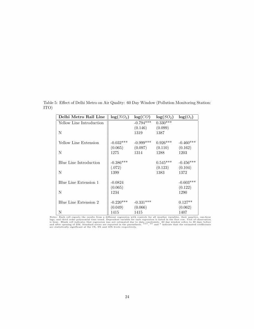
Table 5: Effect of Delhi Metro on Air Quality: 60 Day Window (Pollution Monitoring Station:ITO)

Delhi Metro Rail Line log(NO2) log(CO) log(SO2) log(O3)

Yellow Line Introduction -0.794*** 0.330***(0.146) (0.099)

N 1319 1387

Yellow Line Extension -0.032*** -0.999*** 0.926*** -0.460***(0.065) (0.097) (0.110) (0.162)

N 1275 1314 1288 1203

Blue Line Introduction -0.386*** 0.545*** -0.456***(.072) (0.123) (0.104)

N 1399 1383 1372

Blue Line Extension 1 -0.0824 -0.603***(0.065) (0.122)

N 1234 1290

Blue Line Extension 2 -0.220*** -0.331*** 0.127**(0.049) (0.066) (0.062)

N 1415 1415 1407Notes: Each cell reports the results from a different regression with controls for all weather variables, their quartics, one-hourlags, and third order polynomial time trend. Dependent variable for each regression is listed in the first row. Unit of observationis hour. Blank cell indicates that regression was not estimated due to data constraints. 60 day window refers to 30 days beforeand after opening of DM. Standard errors are reported in the parenthesis. ∗∗∗, ∗∗ and ∗ indicate that the estimated coefficientsare statistically significant at the 1%, 5% and 10% levels respectively.

24

Table 6: Effect of Delhi Metro on Air Quality: 60 Day Window (Pollution Monitoring Station:Siri Fort)


Yellow Line Introduction -0.474*** -1.811*** 0.225**(0.048) (0.123) (0.094)

N 1366 1380 1381

Yellow Line Extension -0.130(0.081)

N 1209

Blue Line Extension 1 -0.149*(0.083)

N 1286

Blue Line Extension 2 -0.465*** -0.314*** -0.265(0.061) (0.099) (0.087)

N 1409 1342 1369Notes: Each cell reports the results from a different regression with controls for all weather variables, their quartics, one-hourlags, and third order polynomial time trend. Dependent variable for each regression is listed in the first row. Unit of observationis hour. Blank cell indicates that regression was not estimated due to data constraints. 60 day window refers to 30 days beforeand after opening of DM. Standard errors are reported in the parenthesis. ∗∗∗, ∗∗ and ∗ indicate that the estimated coefficientsare statistically significant at the 1%, 5% and 10% levels respectively.

Table 7: Effect of Delhi Metro on Air Quality: 60 Day Window (Pollution Monitoring Station:DCE)


Blue Line Extension 1 0.176* 0.034 -0.007 -0.391***(0.093) (0.030) (0.203) (0.037)

N 1272 1338 1331 1337

Blue Line Extension 2 1.778 -0.073 0.165 0.100(0.154) (0.046) (0.131) (0.111)

N 1369 1375 1370 1367Notes: Each cell reports the results from a different regression with controls for all weather variables, their quartics, one-hourlags, and third order polynomial time trend. Dependent variable for each regression is listed in the first row. Unit of observationis hour. Blank cell indicates that regression was not estimated due to data constraints. 60 day window refers to 30 days beforeand after opening of DM. Standard errors are reported in the parenthesis. ∗∗∗, ∗∗ and ∗ indicate that the estimated coefficientsare statistically significant at the 1%, 5% and 10% levels respectively.

25

Table 8: Effect of Delhi Metro on Air Quality: 60 Day Window Model with Lagged OutcomeVariables (Pollution Monitoring Station: ITO)


Yellow Line Introduction -0.106*** 0.094(0.070) (0.069)

N 1299 1356

Yellow Line Extension -0.013 -0.183*** 0.272*** -0.099(0.049) (0.056) (0.087) (0.115)

N 1228 1290 1208 1117

Blue Line Introduction -0.047 0.118* -0.109*(.036) (0.071) (0.061)

N 1391 1328 1332

Blue Line Extension 1 0.008 -0.173*(0.040) (0.089)

N 1177 1241

Blue Line Extension 2 -0.053** -0.074** 0.047(0.026) (0.032) (0.043)

N 1411 1411 1379Notes: Each cell reports the results from a different regression with controls for all weather variables, their quartics, one-hour lags,and third order polynomial time trend. Regressions reported here also control for all four lags of outcome variable. Dependentvariable for each regression is listed in the first row. Unit of observation is hour. Blank cell indicates that regression was notestimated due to data constraints. 60 day window refers to 30 days before and after opening of DM. Standard errors are reportedin the parenthesis. ∗∗∗, ∗∗ and ∗ indicate that the estimated coefficients are statistically significant at the 1%, 5% and 10% levelsrespectively.

26

Table 9: Effect of Delhi Metro on Air Quality: 60 Day Window Model with Lagged OutcomeVariables (Pollution Monitoring Station Data: Siri Fort)


Yellow Line Introduction -0.074*** -0.204*** 0.020(0.029) (0.064) (0.102)

N 1334 1364 1365

Yellow Line Extension -0.025(0.055)

N 1133

Blue Line Extension 1 -0.007(0.054)

N 1215

Blue Line Extension 2 -0.065** -0.075 -0.070(0.028) (0.055) (0.048)

N 1397 1274 1307Notes: Each cell reports the results from a different regression with controls for all weather variables, their quartics, one-hour lags,and third order polynomial time trend. Regressions reported here also control for all four lags of outcome variable. Dependentvariable for each regression is listed in the first row. Unit of observation is hour. Blank cell indicates that regression was notestimated due to data constraints. 60 day window refers to 30 days before and after opening of DM. Standard errors are reportedin the parenthesis. ∗∗∗, ∗∗ and ∗ indicate that the estimated coefficients are statistically significant at the 1%, 5% and 10% levelsrespectively.

Table 10: Effect of Delhi Metro on Air Quality: 60 Day Window with Lagged OutcomeVariables (Pollution Monitoring Station: DCE)


Blue Line Extension 1 0.049 0.008 0.027 -0.033(0.067) (0.017) (0.138) (0.020)

N 1216 1326 1311 1329

Blue Line Extension 2 0.122* -0.018 -0.009 0.026(0.065) (0.021) (0.066) (0.081)

N 1345 1359 1342 1339Notes: Each cell reports the results from a different regression with controls for all weather variables, their quartics, one-hour lags,and third order polynomial time trend. Regressions reported here also control for all four lags of outcome variable. Dependentvariable for each regression is listed in the first row. Unit of observation is hour. Blank cell indicates that regression was notestimated due to data constraints. 60 day window refers to 30 days before and after opening of DM. Standard errors are reportedin the parenthesis. ∗∗∗, ∗∗ and ∗ indicate that the estimated coefficients are statistically significant at the 1%, 5% and 10% levelsrespectively.

27

Table 11: Effect of Delhi Metro on Air Quality: Longer Time Window (Pollution MonitoringStation: ITO)


Yellow Line Introduction 0.002 -0.611***(0.065) (0.060)

N 3965 6840

Yellow Line Extension -0.260*** -0.429***(0.064) (0.062)

N 6956 6823

Blue Line Introduction -0.026 0.883*** -0.508***(.052) (0.089) (0.077)

N 2544 2732 2715

Blue Line Extension 1 0.187*** -0.490***(0.055) (0.088)

N 2486 2526

Blue Line Extension 2 -0.286*** -0.105**(0.048) (0.048)

N 2349 2260Notes: Each cell reports the results from a different regression with controls for all weather variables, their quartics, one-hour lags,and third order polynomial time trend. Time windows for each cell differ. This information is provided in Table 2. Dependentvariable for each regression is listed in the first row. Unit of observation is hour. Blank cell indicates that regression was notestimated due to data constraints. Standard errors are reported in the parenthesis. ∗∗∗, ∗∗ and ∗ indicate that the estimatedcoefficients are statistically significant at the 1%, 5% and 10% levels respectively.

Table 12: Effect of Delhi Metro on Air Quality: Longer Time Window (Pollution MonitoringStation: Siri Fort)



N 2856 2747

Blue Line Extension 2 -0.280*** -0.091 -0.601***(0.048) (0.075) (0.065)

N 2344 2267 2292Notes: Each cell reports the results from a different regression with controls for all weather variables, their quartics, one-hourlags, and third order polynomial time trend. Time window is two months before and after DM open data for each cell. Dependentvariable for each regression is listed in the first row. Unit of observation is hour. Blank cell indicates that regression was notestimated due to data constraints. Standard errors are reported in the parenthesis. ∗∗∗, ∗∗ and ∗ indicate that the estimatedcoefficients are statistically significant at the 1%, 5% and 10% levels respectively.

28

Table 13: Effect of Delhi Metro on Air Quality: 60 Day Window


Average Across All Stations

Blue Line Extension 2 -0.227*** -0.230***(0.047) (0.059)

N 1361 1307Average Across ITO and DCE

Blue Line Extension 1 -0.017 -0.364***(0.066) (0.038)

N 1164 1284

Blue Line Extension 2 0.088(0.079)

N 1358Average Across ITO and Siri Fort

Yellow Line Introduction -0.298***(0.087)

N 1351

Yellow Line Extension 0.570***(0.086)

N 1117

Blue Line Extension 2 -0.347***(0.071)

N 1341Notes: Each cell reports the results from a different regression with controls for all weather variables, their quartics, one-hour lags,and third order polynomial time trend. Dependent variable for each regression is listed in the first row. Unit of observation is hour.Blank cell indicates that regression was not estimated due to data constraints. Standard errors are reported in the parenthesis.∗∗∗, ∗∗ and ∗ indicate that the estimated coefficients are statistically significant at the 1%, 5% and 10% levels respectively.

Table 14: Effect of Delhi Metro on CO: Longest Time Window (Monitoring Station: ITO)

Delhi Metro Rail Line Model with no Lags Model with Lags


Yellow Line Extension -0.128** 0.002(0.047) (0.024)

N 8448 8328Notes: First column reports the regression run with data from September 2004 to October 2005. It includes both discontinuitiesthat occurred in this time period along with controls for all weather variables, their quartics, one-hour lags, and third orderpolynomial time trend. Regression results reported in third column, in addition, control for all four lags of outcome variable. Unitof observation is hour. Standard errors are reported in the parenthesis. ∗∗∗, ∗∗ and ∗ indicate that the estimated coefficients arestatistically significant at the 1%, 5% and 10% levels respectively.

29

Table 15: Effect of Delhi Metro on SO2: Longest Time Window (Pollution Monitoring Station:ITO)

Delhi Metro Rail Line Model without Lags Model with Lags

Yellow Line Introduction -0.169*** -0.033(0.060) (0.034)

Yellow Line Extension -1.068*** -0.198***(0.055) (0.032)

Blue Line Introduction 0.293*** 0.085***(0.063) (0.035)

N 10,877 10,519Notes: First column reports the regression run with data from October 2004 to March 2006. It includes all three discontinuities inthis time period along with controls for all weather variables, their quartics, one-hour lags, and third order polynomial time trend.Regression results reported in third column, in addition, control for all four lags of outcome variable. Unit of observation is hour.Standard errors are reported in the parenthesis. ∗∗∗, ∗∗ and ∗ indicate that the estimated coefficients are statistically significantat the 1%, 5% and 10% levels respectively.

30

Figure 1: Map of the Delhi Metro

31

Figure 2: Delhi Metro Ridership During 2004-2006

Figure 3: Percentage Change in Delhi Metro Ridership During 2004-2006

32

Figure 4: Concentration of Nitrogen Dioxide During 2004-2006

Figure 5: Concentration of Carbon Monoxide During 2004-2006

33

Figure 6: Concentration of Sulphur Dioxide During 2004-2006

Figure 7: Concentration of Ozone During 2004-2006

34

THE EFFECT OF METRO RAIL ON AIR POLLUTION IN DELHI Effect of Metro... · THE EFFECT OF METRO RAIL...

Documents

Transcript of THE EFFECT OF METRO RAIL ON AIR POLLUTION IN DELHI Effect of Metro... · THE EFFECT OF METRO RAIL...