THE EFFECT OF FISCAL POLICY ON THE PERFORMANCE

OF THE NAIROBI SECURITIES EXCHANGE

CECILIA MUYANGA

D61/68123/2011

A RESEARCH PROJECT SUBMITTED IN PARTIAL

FULFILMENT OF THE REQUIREMENTS FOR AWARD OF THE

DEGREE OF MASTER OF BUSINESS ADMINISTRATION,

UNIVERSITY OF NAIROBI

OCTOBER 2014

ii

DECLARATION

This research project is my original work and has not been submitted for examination

in any other university.

Signature: ........................................ Date: ............................................

CECILIA MUYANGA D61/68123/2011

This research project has been submitted for examination with my approval as a

university supervisor.

Signature: .......................................... Date: ...................................

MR. MIRIE MWANGI

Supervisor,

Department of Finance and Accounting,

School of Business, University of Nairobi

iii

ACKNOWLEDGEMENT

I would like to extend my deepest gratitude to the Almighty God who gave me the

strength, protection and ability to undertake this project.

My supervisor Mr. Mirie, I am forever grateful for the support you gave me. This

work was demanding but you were ever at my disposal for advice and guidance.

I wish to acknowledge the good efforts of the Central Bank of Kenya, the Nairobi

Securities Exchange and Kenya National Bureau of Statistics for compiling the data

that makes work easy for researchers like myself. Without the good work of these

government agencies, this piece of work would have been difficult to undertake.

I also wish to deeply thank my caring and loving mother, Jemimah Muyanga who

encouraged me and prayed for me throughout the time of my MBA programme.

Lastly, but by no means the least, to my dear and supportive husband and children,

your support, encouragement, prayers and patience for my absence cannot escape my

attention. You were a constant source of inspiration to me; you gave me drive and

discipline to tackle this task with enthusiasm and determination. Without your love

and support this project would not have been made possible.

May the Almighty God richly bless all of you.

iv

DEDICATION

I dedicate this work to my best friend and husband, Tom Kilonzo and my wonderful

children Austin Mwendwa and Justine Mwende for being there for me throughout the

entire MBA program. Three of you have been my best cheerleaders.

Above all, to God who did it all.

v

TABLE OF CONTENTS

DECLARATION......................................................................................................... ii

ACKNOWLEDGEMENT ......................................................................................... iii

DEDICATION............................................................................................................ iv

LIST OF TABLES .................................................................................................... vii

LIST OF FIGURES ................................................................................................. viii

ABBREVIATIONS .................................................................................................... ix

ABSTRACT ..................................................................................................................x

CHAPTER ONE ..........................................................................................................1

INTRODUCTION........................................................................................................1

1.1 Background of the Study ......................................................................................1

1.1.1 Fiscal Policy ..................................................................................................2

1.1.2 Performance of Securities Exchange .............................................................4

1.1.3 Relationship Between Fiscal Policy and Stock Market Performance ...........6

1.14 Fiscal Policy in Kenya and the Nairobi Securities Exchange ........................8

1.2 Research Problem ...............................................................................................11

1.3 Research Objective .............................................................................................13

1.4 Value of the Study ..............................................................................................13

CHAPTER TWO .......................................................................................................14

LITERATURE REVIEW .........................................................................................14

2.1 Introduction ........................................................................................................14

2.2 Theoretical Review ............................................................................................14

2.2.1 Efficient Markets Hypothesis ......................................................................14

2.2.2 Keynes’ Theory of Consumption ................................................................16

2.3 Determinants of Performance of Securities Exchanges .....................................18

2.4 Empirical Literature ...........................................................................................20

2.5 Summary of Literature Review ..........................................................................27

CHAPTER THREE ...................................................................................................29

RESEARCH METHODOLOGY .............................................................................29

3.1 Research Design .................................................................................................29

3.2 Population ...........................................................................................................29

3.3 Study Sample ......................................................................................................29

vi

3.4 Data Collection ...................................................................................................30

3.5 Data Analysis .....................................................................................................30

CHAPTER FOUR ......................................................................................................33

DATA ANALYSIS, RESULTS AND DISCUSSION ..............................................33

4.1 Introduction ........................................................................................................33

4.2 Descriptive Statistics ..........................................................................................33

4.3 Correlation of Analysis ......................................................................................35

4.4 Linear Regression Modelling .............................................................................36

4.4.1 Error Correction ..........................................................................................40

4.5 Discussion of Research Findings .......................................................................44

CHAPTER FIVE .......................................................................................................47

SUMMARY, CONCLUSION AND RECOMMENDATIONS .............................47

5.1 Introduction ........................................................................................................47

5.2 Summary of Findings .........................................................................................47

5.3 Conclusion ..........................................................................................................48

5.4 Recommendations ..............................................................................................50

5.5 Limitations of the Study .....................................................................................50

5.6 Suggestions for Further Research ......................................................................51

REFERENCES ...........................................................................................................52

APPENDICES ............................................................................................................62

Appendix I: Multiple Line Graphs ...........................................................................62

Appendix II: Q-Q Plots ............................................................................................63

Appendix III: Differenced Variables ........................................................................64

Appendix IV: Study Data .........................................................................................65

vii

LIST OF TABLES

Table 4.1: Descriptive Statistics Results ........................................................................... 33

Table 4.2: Correlation Matrix ........................................................................................... 36

Table 4.3: Model Summary .............................................................................................. 37

Table 4.4: Analysis of Variance........................................................................................ 37

Table 4.5: Regression Coefficients ................................................................................... 38

Table 4.6: Model Summary – Error Corrected ................................................................. 41

Table 4.7: Analysis of Variance – Error Corrected .......................................................... 41

Table 4.8: Corrected Regression Model – Error Corrected .............................................. 42

viii

LIST OF FIGURES

Figure 4.1: CUSUM Test for Parameter Stability ............................................................ 39

Figure 4.2: Residual Graph ............................................................................................... 44

ix

ABBREVIATIONS

ADF - Augmented Dickey Fuller

AIMS – Alternative Investment Market Segment

CBK - Central Bank of Kenya

CPI – Consumer Price Index

CUSUM - Cumulative Sum Chart

EMH – Efficient Market Hypothesis

FDI – Foreign Direct Investment

FIMS – Fixed Income Market Segment

GDP – Gross Domestic Product

KNBS – Kenya National Bureau of Statistics

KRA – Kenya Revenue Authority

LIC – Low Income Countries

MIMS – Main Investment Market Segment

MPC – Marginal Propensity to Consume

NASI - Nairobi All Share Index

NSE – Nairobi Securities Exchange

OECD – Organization for Economic Co-operation and Development

VIF - Variance Inflation Factors

x

ABSTRACT

The aim of this descriptive and correlational study was to determine the relationship

between fiscal policy and performance of the Nairobi Securities Exchange. The

performance measure of the Nairobi Securities Exchange used was the NSE 20-Share

Index which was regressed against the fiscal policy instruments including government

revenue, government expenditure and government debt expressed as percentage of the

GDP. The period of the study was ten years from January 2004 to December 2013.

The study employed monthly secondary data which was obtained from the CBK,

Kenya National Bureau of Statistics and NSE. Data were analyzed using the Ordinary

Least Square method which assumes linearity between the dependent variable and the

independent variables and the analysis technique was multiple regression aided by

research software ‘eviews’ version 7. The study found out that performance of the

stock market is influenced by the Government’s fiscal policies. Government

expenditure and revenue had positive effect on stock market performance as both are

indicative of the economic performance and the former reflect micro and

macroeconomic consideration and direction of the Government. Government debt had

low positive effect on stock market performance with a negative cumulative effect as

its long-term use poses risk of inflation owing to interest rates on debt. These findings

confirm the researcher’s priori expectation that government fiscal policy actions

significantly affect stock performance. The rest of the paper is organized as follows:

chapter one covers introduction by addressing issues related to background of the

study, statement of the problem, study objective and the significance of the study;

chapter two focuses on literature review; chapter three is about the research

methodology; chapter four covers data analysis, results and discussion; and lastly

chapter five addresses summary, conclusion and recommendations.

1

CHAPTER ONE

INTRODUCTION

1.1 Background of the Study

One of the factors that helps determine the country's economic direction is fiscal

policy. The government uses fiscal policy to influence the economy by adjusting

revenue and spending levels (Afonso and Sousa, 2011). Fiscal policy is based on the

theories of British economist John Maynard Keynes, which state that increasing or

decreasing revenue (taxes) and expenditures (spending) levels influences inflation,

employment and the flow of money through the economic system. Fiscal policy is

often used in combination with monetary policy, which is set to influence the

direction of the economy and meet economic goals (Steven, 2003).

The two main tools of fiscal policy are taxes and spending. Taxes influence the

economy by determining how much money the government has to spend in certain

areas and how much money individuals have to spend. For example, if the

government is trying to spur spending among consumers, it can decrease taxes. A cut

in taxes provides families with extra money, which the government hopes they will

turn around and spend on other goods and services, thus spurring the economy as a

whole (Heyne et al, 2002).

Spending is used as a tool for fiscal policy to drive government money to certain

sectors that need an economic boost. Whoever receives those dollars will have extra

2

money to spend – and, as with taxes, the government hopes that money will be spent

on other goods and services. The key is finding the right balance and making sure the

economy doesn't lean too far either way. There are two main types of fiscal policy:

expansionary and contractionary; Expansionary fiscal policy, designed to stimulate

the economy, is most often used during a recession, times of high unemployment or

other low periods of the business cycle. It entails the government spending more

money, lowering taxes, or both. The goal is to put more money in the hands of

consumers so they spend more and stimulate the economy (Steven, 2003).

Contractionary fiscal policy is used to slow down economic growth, such as when

inflation is growing too rapidly. The opposite of expansionary fiscal policy,

contractionary fiscal policy raises taxes and cuts spending.

1.1.1 Fiscal Policy

Fiscal policy involves the use of government spending, taxation and borrowing to

affect the level and growth of aggregate demand, output and jobs. Fiscal policy is also

used to change the pattern of spending on goods and services. It is also a means by

which a redistribution of income & wealth can be achieved. It is an instrument of

intervention to correct for free-market failures (Heyne et al, 2002).

Traditionally fiscal policy has been seen as an instrument of demand management.

This means that changes in government spending, direct and indirect taxation and the

budget balance can be used “counter-cyclically” to help smooth out some of the

3

volatility of national output particularly when the economy has experienced an

external shock and is in a recession (Steven, 2003).

The Keynesian school argues that fiscal policy can have powerful effects on demand,

output and employment when the economy is operating below full capacity national

output, and where there is a need to provide a demand-stimulus. Monetarist

economists believe that government spending and tax changes only have a temporary

effect on aggregate demand, output and jobs and that the tools of monetary policy are

a more effective instrument in controlling inflation and maintaining macroeconomic

stability (Steven, 2003).

The government uses fiscal policy to promote economic growth, low unemployment

and to stabilize the economy. During period of low economic growth, the government

tends to cut taxes and may increase spending in an attempt to spark growth. During

periods of high economic growth, the government may increase taxes and cut

spending to ensure that the economy doesn't grow too quickly which can result in

undesirable effects like high inflation. The main instruments of fiscal policy are

discussed in the subsequent paragraphs.

Taxation is one of the two primary instruments of fiscal policy. When the government

increases or decreases taxes, it increases or decreases the amount of money consumers

have to spend which can have a significant impact on the direction of the overall

economy. A decrease in taxation tends to put more money into the hands of

consumers, which can lead to increased spending. Increased spending tends to lead to

4

higher revenues for businesses, which can allow them to expand and hire more

workers. Cutting taxes is a common fiscal policy measure to encourage economic

growth (Heyne et al, 2002).

Government spending is the other main instrument of fiscal policy. The expenditures

of the government can promote economic activity and create jobs. For example, if the

government funds a project to build a high-speed train across the country, the funds

that go into the project could go toward hiring workers which could reduce

unemployment and inject money into the economy. Higher levels of government

spending tend to promote employment and economic growth (Larch and Nogueira,

2009)

Reducing taxes and increasing spending can both promote economic growth, but if

the government spends more than it takes in through taxes it is operating on a deficit,

meaning it is losing money over time. Operating on a deficit causes the government to

accumulate debt (Heyne et al, 2002).

1.1.2 Performance of Securities Exchange

Godspeed (2008) defines stock market as the institutional framework through which

public companies issue new share capital in the primary market and the ownership of

the shares changes hands in the secondary market. Mishkin (2007) defines a stock as a

security that is claimed on the earnings and assets of corporations. Stocks are sold in a

formal market called the stock exchange. Economic agents buy shares because they

value the dividends that their investments will pay in future. Equity stock not only

5

pays a dividend but also capital gains if the owner transfers ownership in the

secondary market.

Common stock markets in the world include S and P 500 in the United States, the

FTSE 100 in the United Kingdom, the Nikkei Stock Average in Japan, the Hang Seng

in Hong Kong, DAX in Germany, CAC 40 in France, Bovespa in Brazil to mention a

few while NSE is the Kenya’s stock market. Filis (2010) opined that stock market is

the best indicator to forecast future economic activities and describe the actual causal

effect between future economic growth and stock prices.

The existence of the stock market enables individual investors to transfer the control

of their savings to the market place with confidence. Individual investors exchange

their savings for shares of companies that are listed on the stock exchange. The share

gives the individuals the right to vote and appoint directors of the company who have

the responsibility of steering the performance of the company. If the company is

doing well the shareholders are entitled to a return on their investment in form of a

dividend on each share held. Management has to perform adequately and

satisfactorily or they will have to be replaced by competent managers. Shareholders

therefore keep a firm grip on management so that they at least try to guarantee a

return on their investment (Pilbeam, 1998).

Stock markets promote higher standards of accounting, resource management and

transparency in the management of business. This is because financial markets

encourage the separation of owners of capital, on the one hand, from managers of

6

capital, on the other. The stock exchange also improves the access to finance of

different types of users by providing the flexibility for customization. Lastly the stock

exchange provides investors with an efficient mechanism to liquidate their

investments in securities. The very fact that investors are certain of the possibility of

selling out what they hold, as and when they want, is a major incentive for investment

as it guarantees mobility of capital in the purchase of assets (www.nse.co.ke).

1.1.3 Relationship Between Fiscal Policy and Stock Market

Performance

Some observers view the stock market as an independent source of macroeconomic

volatility to which policymakers may wish to respond (Bernanke and Kuttner, 2005).

Fiscal measures enacted by various agencies of national governments influence the

aggregate economies of those countries. The resulting economic conditions influence

all industries and companies in an economy positively or negatively which in turn

affect the performance of stock markets (Fama, 1970).

Even though a significant number of past studies have concentrated their attention on

the relationship between monetary policy and stock market performance (Fama and

French, 1988), only few investigate the effects of fiscal policy on stock markets

(Darrat, 1994; Afonso and Sousa, 2011).

Fiscal policy used in a Keynesian manner can support aggregate demand, boosting the

economy and potentially driving stock prices higher. In contrast, classical economic

theory focuses on the crowding out effects of fiscal policy in the market for loanable

7

funds and of the productive sectors of the economy. Hence, fiscal policy could

potentially drive stock prices lower through the crowding out of private sector

activity. Furthermore, from a Ricardian perspective (Barro, 1974; Barro, 1979) fiscal

policy is impotent and as such will have no effect on stock markets.

Theoretically, fiscal policy actions (changes in expenditures or taxes resulting in

budget deficits or surpluses) play a significant role in the determination of asset

prices. For example, increases in taxes, with government spending unchanged, would

lower (expected) asset returns (or prices) as they discourage investors from (further)

investing in the stock market (Afonso and Sousa, 2011).

Increases in government borrowing raise the (short-term) interest rate which, in turn,

lower the discounted cash flow value from an asset (like a share) and thus signals a

reduction in stock market activity (aside from other adverse effects in the general

economy) (Barro, 1974,1979).

The priori expectation of this study is that fiscal policy affects the performance of the

stock market as a critical component of the economy. Moreover, the researcher

expects that various monetary policy instruments stated in the model as independent

variables will be correlated to the NSE 20-share index differently either positively or

negatively.

8

1.14 Fiscal Policy in Kenya and the Nairobi Securities Exchange

Fiscal Policy is the use of government revenue collection (taxation) and expenditure

to influence the economy. The government of Kenya uses fiscal policy to influence

the level of aggregate demand in the economy, in an effort to achieve economic

objectives of price stability, full employment and economic growth. Keynesian

economic suggests that increasing government spending and decreasing tax rates are

the best ways to stimulate aggregate demand, and decreasing spending and increasing

taxes after the economic boom begins (Kariuki, 2003).

Kenya’s strong economic performance between 2002 and 2007 has been partly

attributed to macroeconomic stability and strong fiscal consolidation. After two

decades of sluggish performance, economic growth resumed in 2002 and steadily

increased from 0.5 percent to 7 percent in 2007. During this period, the government

retired debt and started creating fiscal space to fund essential infrastructure. The ratio

of debt to Gross Domestic Product (GDP) declined from 60 percent in 2000 to 40

percent in 2008. Fiscal space was achieved through a strong revenue effort and

stringent fiscal management (Kirira, 2009).

The rationale for allocating the budget for development purposes is to upgrade rural

basic infrastructure, urban transport, low income household and other social services.

These expenditure purposes have a significant role in sustaining growth momentum

and positive economic transformation (GOK, 2011). Kenya has been experiencing

fiscal deficit over the years.

9

The Nairobi Securities Exchange (NSE) is the only stock exchange market in Kenya

and is located in Nairobi city. It was formed in 1954 as a voluntary organization of

stock brokers and is now one of the most active capital markets in Africa. As a capital

market institution, the Stock Exchange plays an important role in the process of

economic development. It helps mobilize domestic savings thereby bringing about the

reallocation of financial resources from dormant to active agents. Long-term

investments are made liquid, as the transfer of securities between shareholders is

facilitated. The Exchange has also enabled companies to engage local participation in

their equity, thereby giving Kenyans a chance to own shares (www.nse.co.ke).

Trading at the NSE is automated through the ATS. The products traded are shares and

bonds, with over 50 different types of shares and over 60 bonds. Bonds are in two

groups namely treasury bonds issued by the government and corporate bonds issued

by companies. On the other hand, shares are grouped into four sectors including

agriculture; commercial and services; finance and investment; and industrial and

allied sectors (www.nse.co.ke).

Nairobi Stock Exchange (NSE) is categorized into three market segments; Main

Investment Market Segment (MIMS); Alternative Investment Market Segment

(AIMS); and Fixed Income Market Segment (FIMS). The MIMS is the main

quotation market (www.nse.co.ke).

The NSE 20-Share Index has been in use since 1964 and measures the performance of

20 blue-chip companies with strong fundamentals and which have consistently

10

returned positive financial results. The NSE 20 Share Index (^N20I) is a price weight

index. The members are selected based on a weighted market performance for a 12

month period as follows: Market Capitalization 40%, Shares Traded 30%, Number of

deals 20%, and Turnover 10%. Index is updated end of day only. Included in the

Index are Mumias Sugar, Express Kenya, Rea Vipingo, Sasini Tea, CMC Holdings,

Kenya Airways, Safaricom, Nation Media Group, Barclays Bank Kenya, Equity

Bank, Kenya Commercial Bank, Standard Chartered Bank, Bamburi Cement, British

American Tobacco, Kengen, Centum Investment Company, East African Breweries,

EA Cables, Kenya Power & Lighting Company Ltd. and Athi River Mining. This

index primarily focuses on price changes amongst these 20 companies

(www.mystocks.co.ke).

The NSE 20-Share Index is the long-standing benchmark index used for equities

traded on the NSE and represents the geometric mean of share prices of the NSE's 20

top stocks. It has recently been joined by the more broad-based NSE All Share Index

(NASI), aimed at capturing the market capitalization of all the NSE's listed equities

traded in a day. The NSE 20 lost more than one-third of its value in 2008 as the

investors began fleeing stocks after brokerage collapses and the global credit crisis

(www.nse.co.ke). Other measures of stock performance used at the NSE include

market capitalization and equity turnover.

Several studies carried out on the stock market performance in Kenya have used the

NSE 20-share index as a measure of the NSE performance. Some of these studies

11

include (Nyamute, 1998; Mutoko, 2006; and Siele, 2009). The current study will use

the NSE-20 share index as a measure of the stock market performance as well.

1.2 Research Problem

Fiscal policy used in a Keynesian manner can support aggregate demand, boosting the

economy and potentially driving stock prices higher. In contrast, classical economic

theory focuses on the crowding out effects of fiscal policy in the market for loanable

funds and of the productive sectors of the economy. Hence, fiscal policy could

potentially drive stock prices lower through the crowding out of private sector

activity. Furthermore, from a Ricardian perspective (Barro, 1974, 1979) fiscal policy

is impotent and as such will have no effect on stock markets. Fiscal policy actions

(changes in expenditures or taxes resulting in budget deficits or surpluses) play a

significant role in the determination of asset prices. For example, increases in taxes,

with government spending unchanged, would lower (expected) asset returns (or

prices) as they discourage investors from (further) investing in the stock market

(Afonso and Sousa, 2011).

Globally, various researchers have examined fiscal policy in quite a number of

perspectives, for instance, Hondroyiannis and Papapetrou (2001) examined

macroeconomic influences on the stock market for Greece. They found that stock

prices do not lead changes in real economic activity but that the macroeconomic

activity and foreign stock market changes only partially explained Greek stock price

movements. Fuente (1997) examined the impact of public expenditures and taxation

on economic growth of 21 OECD countries from 1965 to 1995. The results of the

12

study could not provide evidence in support of fiscal policy led growth. Specifically,

public expenditures tend to crow out private investment leading to reduction in

disposable income and incentive to save. Devarajan et al (1996) and Afonso and

Furceri (2010) found that government investment has sizable negative and statistically

significant effect on growth.

Locally, Nkukuu (2011) examined the impact of government budget balance on the

stock market return and found a weak negative relationship. Bhujbal (2012) on the

other hand examined the relationship between local government expenditure and

inter-governmental fiscal transfer and found that the local government expenditure is

positive and significantly influence the inter-government fiscal transfer. Njenga

(2012) looked at the relationship between fiscal Policy and Public Investment in

Kenya and noted that a positive change in Government Capital Expenditure would

lead to an increase in public investments. The study concluded that low-income

countries such as Kenya fiscal policies may not be harmful for either long- or short-

term growth.

To the best of the researcher’s knowledge, there are no studies related to the

performance of Nairobi Securities Exchange and fiscal policy variables. This

strengthens the importance of the current study and the value it adds to the existing

literature. Therefore, this paper aims to examine the relationship between fiscal policy

and performance of the stock market for the ten year period between 2004 and 2013.

13

1.3 Research Objective

The study sought to establish the effect of fiscal policy on the performance of the

Nairobi Securities Exchange.

1.4 Value of the Study

This study will benefit researchers and academicians in finding more evidence on the

determinants of the performance of the Nairobi Securities Exchange. Scholars and

academicians will find this study a useful guide for the same as it will recommend on

areas for further research. The current study will also further help investors to

proactively strategize their investment decisions.

The findings of this study would help the policy makers or regulatory bodies

understand the behaviour of the stock market and benefit the information toward

achieving fiscal goals. It will enable them understand the growing need to formulate

fiscal policies that will be responsive to changes in NSE 20-share index, since the

stock market is a veritable source of long-term capital. The effectiveness of fiscal

policy should therefore be anchored on the potency of its instruments on stock market

performance.

14

CHAPTER TWO

LITERATURE REVIEW

2.1 Introduction

This chapter presents the literature review on the subject under study as presented by

various researchers and scholars. The review has drawn materials from several

sources that are closely related to the theme and objective of the study. The chapter

contains three areas as follows: first, theoretical review; second, empirical studies;

and third, conclusions from literature review.

2.2 Theoretical Review

The basis of the study rests on the following theories:

2.2.1 Efficient Markets Hypothesis

Efficient market hypothesis (EMH) postulates that any new information is quickly

and efficiently incorporated into asset prices at any point in time, so that old

information cannot be used to foretell future price movements. Fama (1965b) first

defined the term "efficient market" as one in which security prices fully reflects all

available information. The market is efficient if the reaction of market prices to new

information should be instantaneous and unbiased.

Three versions of EMH have been advanced. The weak form EMH stipulates that

current asset prices already reflect past price and volume information. The

15

information contained in the past sequence of prices of a security is fully reflected in

the current market price of that security. It is named weak form because the security

prices are the most publicly and easily accessible pieces of information. It implies that

no one should be able to outperform the market using the available information" Fama

(1965a; 1965b)

The semi strong form EMH states that all publicly available information is similarly

already incorporated into asset prices. In other words, all publicly available

information is fully reflected in a security's current market price. The public

information stated not only past prices but also data reported in a company's financial

statements, company's announcement, economic factors and others. It also implies

that no one should be able to outperform the market using any information that is

public knowledge Fama (1965a).

The strong form EMH stipulates that private information or insider information too, is

quickly incorporated by market prices and therefore cannot be used to reap abnormal

trading profits. Thus, all information, whether public or private, is fully reflected in a

security's current market price. That means even the company's management

considered as insiders are not able to make gains from inside information they hold.

They are not able to take the advantages to profit from information such as ‘take over

decisions’ which has been made ten minutes ago. The rationale behind this is that the

market anticipates, in an unbiased manner, future development and therefore

information has been incorporated and evaluated into market price in a much more

objective and informative way than insiders, French and Roll (1986).

16

Therefore if all fiscal actions of government are publicly known it implies that no one

should be able to outperform the market using something that "everybody else

knows". Similarly, it means that all this information will be incorporated in the

securities prices. Hence when government reduce taxes in an expansionary fiscal

policy, activity at NSE is expected to increase hence higher security prices and vice

versa.

2.2.2 Keynes’ Theory of Consumption

The Keynesian Theory of consumption is that current real disposable income is the

most important determinant of consumption in the short run. Real Income is money

income adjusted for inflation. It is a measure of the quantity of goods and services that

consumers have bought with their income (or budget) (Keynes, 1936). For example, a

10% rise in money income may be matched by a 10% rise in inflation. This means

that real income (the quantity or volume of goods and services that can be bought) has

remained constant.

The standard Keynesian consumption function is as follows:

C = a + c Yd where,

C= Consumer expenditure

a = autonomous consumption. This is the level of consumption that would take place

even if income was zero. If an individual's income fell to zero some of his existing

17

spending could be sustained by using savings. This is known as dis-saving (Keynes,

1936).

c = marginal propensity to consume (mpc). This is the change in consumption divided

by the change in income. Simply, it is the percentage of each additional pound earned

that will be spent.

There is a positive relationship between disposable income (Yd) and consumer

spending. The gradient of the consumption curve gives the marginal propensity to

consume. As income rises, so does total consumer demand (Keynes, 1936).A change

in the marginal propensity to consume causes a pivotal change in the consumption

function. In this case the marginal propensity to consume has fallen leading to a fall in

consumption at each level of income. According to Keynes’s theory, aggregate

consumption was a positive but diminishing function of aggregate income

(Veganzones, 2005).

Consumption is, or shall be defined to be, the total quantity of goods and services that

people in the economy wish to purchase for the purpose of immediate consumption.

As such, it is one of the main determinants of an economy’s aggregate demand (that

is, the sum of all planned expenditures in the economy). Other determinants of

aggregate demand include investment and government expenditure (with net trade

taken into account for open markets), which are also defined in terms of desired rather

than actual expenditure (Mishkin, 1996).

18

One place the public can spend more is in the stock market, increasing the demand for

equities and consequently raising their prices (Mishkin, 1996). A more Keynesian

view comes to a similar conclusion because it sees the fall in government expenditure

and increases in taxes stemming from contractionary fiscal policy, this reduces

activity at the NSE and fall in equity prices and vice versa.

2.3 Determinants of Performance of Securities Exchanges

Motivated by growing theoretical evidence, which shows that stock markets play a

vital role in boosting long-run economic growth, governments the world over have

instituted measures aimed at enhancing stock market operations (Blancahrd and

Giavazzi, 2003). However, if any stock market is to play its allocative role properly,

alot more needs to be done on the macroeconomic policy framework front.

Specifically, both fiscal and monetary policies formulation should be geared towards

enhancing the efficacy with which resources are mobilized through the stock market

(Veganzones, 2005).

A number of macroeconomic variables such as changes in interest rate, inflation rates,

and economic growth are believed to affect how stocks perform. The macroeconomic

approach attempts to examine the sensitivity of stock prices to changes in

macroeconomic variables. Under this approach, stock prices are influenced by

changes in money supply, interest rate, inflation and other macroeconomic variables

(Larch and Nogueira, 2009).

19

There are numerous factors having impact on the performance of stock markets, such

as, expansion in the country’s economic activities, strength in the exchange rate,

decrease in lending interest rates and improvement in recovery of outstanding loans,

rescheduling and payment of foreign debts, large scale mergers and acquisitions,

better relationship with the neighbour countries, investor friendly policies and strong

regulatory framework (Imran Ali, 2009).

Stock market performance, economical and political condition of a country is

interrelated and has been a significant debating issue. Many studies directly or

indirectly have been dealing with the macroeconomic and institutional factors and

their correlation with the stock market performance at both theoretical and empirical

levels.

Charles Amo Yarty (2008) found that macroeconomic factors such as income level,

gross domestic investment, banking sector development, private capital flows, stock

market liquidity and institutional determinants such as political risk, law and order,

and bureaucratic quality are important determinants of stock market development in

emerging markets. He used number of listed companies, market capitalization % of

GDP, value traded % of GDP, turnover ratio %, and GDP per capita($) as indicators

of stock market development. Valeriano F. Garcia (1999) also examined the

determinants of stock market development in emerging markets. He found that real

income, saving rate, financial intermediary development and stock market liquidity

are important determinants of stock market capitalization, macroeconomic volatility

20

does not prove significant and stock market development and banking sector

development are complements.

Macroeconomic and institutional, both factors have significant impact on stock

market performance. Valeriano F. Garcia (1999) shows that rules & regulation and

law & order situation of any country have significant impact on stock market

performance. For example, disclosure requirements and investor’s interest protective

regulations increase the investor’s confidence and encourage them to invest and trade

in the stock markets.

2.4 Empirical Literature The impact of fiscal policy on growth has generated large volume of empirical studies

with mixed findings using cross- sectional, time series and panel data. Some of these

studies are country specific while others are cross- country, few of these studied are

selected for review as follows: Fuente (1997) examined the impact of public

expenditures and taxation on economic growth of 21 OECD countries from 1965 to

1995. The results of the study could not provide evidence in support of fiscal policy

led growth. Specifically, public expenditures tend to crow out private investment

leading to reduction in disposable income and incentive to save.

Hondroyiannis and Papapetrou (2001) examined macroeconomic influences on the

stock market for Greece. Among the macroeconomic variables investigated were

interest rates and exchange rates. They found that stock prices do not lead changes in

real economic activity but that the macroeconomic activity and foreign stock market

changes only partially explained Greek stock price movements.

21

Several studies have also examined the underlying reasons for low efficiency of

public investment, with focus on the regional allocation of public investment in Japan.

Variables such as population, area size and income which reflect the scale and

demand for public investment are found to be significant for different types of

investments (Kondoh, 2008). Allocation can also be affected by other policy

objectives such as employment polity or the regional distribution of income.

Devarajan et al. (1996) and Afonso and Furceri (2010) found that government

investment has sizable negative and statistically significant effect on growth. They

conducted the empirical estimation using impulse-response functions and variance

decompositions from a VAR model depending on US stock market data. They

showed that expansionary fiscal policy increases stock returns.

Veganzones (2005) studied determinants of investment in 40 developing economies

using panel data. The results showed that growth anticipations, real interest rate and

government policies explain Middle East’s and North Africa’s low investment rate.

Insufficient structural reforms represented as poor financial development and

deficient trade openness has been a crucial factor for deficit in private capital

formation. Economic uncertainties of the region have constituted major deterrent for

firms to invest. High external debt burden and economic volatility arise primary

reasons for high uncertainty in the region.

Nyamute (1998) sought to analyse whether or not macroeconomic factors affect the

performance of the Nairobi Stock Exchange. The macroeconomic variables taken into

22

account were inflation rate, money supply, interest rates and exchange rates. The

performance of the stock exchange was represented by the movement in the stock

price index. Secondary data was collected from published reports and figures from the

Nairobi Stock exchange, the Central Bank of Kenya and the Central Bureau of

Statistics. This data was analysed by use of multiple regression modelling. The results

of the analysis indicate that macroeconomic variables do indeed impact on the

performance of the stock prices. However, the four macroeconomic variables used in

this study may not be the only ones that affect stock prices. Hence the study

recommends that further research need to be carried out with more variables entered

into the model.

Mongeri (2011) examined the impact of foreign exchange rates and foreign exchange

reserves on stock markets performance at NSE. Monthly time series for NSE share

index, foreign exchange rates and reserves covering the period 2003-2010 were used.

Multiple regression analysis techniques were employed to ascertain long run

relationships between the variables. The study was guided by several theories

including market efficiency theory, classical monetary, portfolio theory and empirical

studies from India, Ghana and Kenya. The study concludes that Foreign exchange

rates and foreign exchange reserves had an impact on the stock performance at NSE.

Foreign exchange rates had negative impact on stock performance which was more

significant. Foreign exchange reserves had positive mpact on stock performance

which was significant. The study also revealed that no significant relationship

between Foreign exchange rates and foreign exchange reserves.

23

The study also shows NSE efficiency is not yet strong even with increased flow of

information at capital market. Further research area can be extended by analyzing

more fundamentals of the Kenyan economy and the stock markets. The major

implication of this study can be for government to use the conclusion to address the

fluctuations of the foreign exchange rate as the empirical result indicate that it has

negative impact in the stock market hence the whole economy. This can be managed

by government through central bank to influence the supply side of exchange rates by

using foreign exchange reserves. Future studies should broaden the study in more than

one country, across regions or within economic blocks e.g. East African community

countries in order to draw stronger conclusions.

Ambunya (2012) did a study to establish the relationship between exchange rate

movement and stock market returns volatility at the Nairobi Securities Exchange. The

study adopted a quantitative design. The target population for this study included 56

companies quoted at the NSE as of December 2011. Since the population was small

and the study is using secondary data, the study conducted a census. The study used

secondary data collected from the Nairobi Securities Exchange and the Central bank

of Kenya for the period 2007-2011. The study regressed stock market returns

volatility against exchange rate movement. From the regression output, the study

established that exchange rate movements greatly affected the stock market return

volatility owing to its information content to the investors. With high fluctuations in

the exchange rates, the exchange rates movement became bigger accompanied by a

24

huge stock market return volatility. Study concludes that there is a strong relationship

between exchange rate movement and stock market returns volatility.

This is especially carried through the information content of exchange rate movement

on the security’s business. The study concludes that exchange rate movement also

affects the stock market performance greatly through its spiral effects. Through over

macroeconomic variables, exchange rate movement indicates the state of the economy

hence the likely future state of the economy. These variables would include things

like interest rate and the money supply in the economy which has great impact on the

activity level of the security’s performance. The policy makers need to factor the

effects of exchange rate movement on the performance of the stock exchange.

Ngigi (2000) investigated the impact of fiscal and monetary policy actions on stock

market performance in Kenya. It sought to answer the question on the nature and

extent of the impact of monetary and fiscal policies on the performance of the NSE. It

further sought to determine which specific components of these policies (anticipated

or unanticipated), affect the NSE performance. The study proceeded by first testing

for stationarity and cointegration of the variables used in the estimation process.

Having specified the fiscal and monetary policies error correction models, it went on

to determine the anticipated and unanticipated components of the same, by use of the

general-to specific model specification and reduction. The values for the anticipated

and unanticipated fiscal and monetary policies attained thereof, were then used in the

estimation of the stock market performance function, as measured by the stock price

index. The empirical results attained showed that both anticipated monetary policy

25

actions, and unanticipated fiscal policy actions affect the stock market negatively,

whilst unanticipated monetary policy adjustments affect it positively. Anticipated

fiscal policy actions on the other hand, were found to have no impact on the stock

market. These findings suggest that policy makers need to exercise considerable

caution regarding fiscal-monetary policy stance and stock market regulation in Kenya

Kariuki (2003) studied the determinants of gross fixed capital formation in Kenya and

found that government expenditure was the most significant determinant. The

research also showed that increases in real interest rates do not deter private sector

private investment while monetary policy plays a less significant role. FDU is very

significant as a determinant of fixed capital formation, while output growth was

insignificant.

Mwanza (2012) conducted a descriptive and correlational study was to determine the

relationship between monetary policy and performance of the Nairobi Securities

Exchange. The Performance measure of the Nairobi Securities Exchange used was the

NSE 20-Share Index which was regressed against the monetary policy instruments

including 91-day Treasury bill rate, exchange rate (US dollar), money supply (M3),

repo rate, cash ratio requirement (CRR) and Central Bank rate (CBR). The period of

the study was six years from June 2006 to June 2012. The study period was relevant

because one of the variables, Central Bank rate (CBR), was introduced in Kenya for

the first time in June 2006 as the rate at which Central Bank of Kenya lends money to

commercial banks through the overnight Lombard window. The study employed

monthly secondary data which was obtained from the Central Bank of Kenya and

26

Nairobi Securities Exchange. Data were analyzed using the Ordinary Least Square

method which assumes linearity between the dependent variable and the independent

variables and the analysis technique was multiple regression aided by research

software “eviews” version 7. The study found that the monetary policy instruments

jointly influenced the variation in the NSE 20-share index with a strong adjusted R2.

Furthermore, the NSE 20-Share Index was found .The rest of the paper is organized as

follows: chapter one covers introduction by addressing issues related to background

of the study, statement of the problem, study objective and the significance of the

study; chapter two focuses on literature review; chapter three is about the research

methodology; chapter four covers data analysis, results and discussion; and lastly

chapter five addresses summary, conclusion and recommendations.

Muchiri (2012) examined the impacts of macroeconomic variables on stock market

performance in the NSE. The study used a descriptive research design. The population

of this study comprised all the 59 listed companies in the Nairobi Securities Exchange

as at 30th June 2012. In this study secondary data was used to investigate the

relationship between independent and dependent variables. The data was analysed

using descriptive analysis, correlation analysis and regression analysis. The study

found that there was a general rise in share prices, money supply, exchange rate,

inflation, and interest rate over the period under study. The study also found that

money supply and inflation rate had positive but insignificant effects on share prices

while interest rate had a negative but insignificant effect on share prices. Further,

exchange rate has a negative and significant effect on share prices. The variables

27

jointly accounted for 95.6% of the variance in share prices. The F statistic was also

significant suggesting that the model was fit to explain the determinants of share

prices. The study concludes that exchange rate has a significant negative impact on

stock market performance. The study recommends that in order for the stock market

performance in Kenya to improve, there is need for the Government to initiate

measures that will control the exchange rate in Kenya. The study also recommends

that there is also need for the Government to control the broad money supply in

Kenya as there is some evidence to suggest that higher money supply may lead to

better stock market performance. The study further recommends that there is need for

the government to initiate policies that will lower the interest rates in Kenya as lower

interest rates may translate to higher stock market performance.

2.5 Summary of Literature Review Fiscal policy affects aggregate demand, distribution of wealth, and the economy’s

capacity to produce goods and services. In the short run, changes in spending or

taxing can alter both magnitude and the pattern of demand for goods and services.

With time, this aggregate demand affects the allocation of resources and the

productive capacity of an economy through its influence on the returns to factors of

production, the development of human capital, the allocation of capital spending, and

investment in the technological innovations (Njenga, 2012).

From the review of the empirical studies very few studies have focused on the

relationship between fiscal policy and stock market behavior. More specifically, these

studies examined primarily stock market efficiency with respect to fiscal actions

28

(Rogalski and Vinso, 1977; Darrat, 1987; Darrat and Brocato, 1994; and Lee, 1997).

No study has investigated empirically how fiscal policy and the stock market have

been interacting intertemporally. However, the theoretical motivation on the effects of

fiscal policy on the stock market (or asset prices) have been laid out more than thirty

years ago (Tobin, 1969; Blanchard, 1981; and Shah, 1984), the empirical front on the

issue has been lagging, both for the US and other countries Darrat, 1987) and Ali and

Hasan, 2003).

The review of literature clearly found a research gap in Kenya as most of the studies

done in the area are conducted in the developed countries and there is still a question

for developing countries like Kenya, regarding the empirical relationship between

fiscal variables and stock market index. The current study therefore seeks to

contribute towards this research gap by establishing the relationship between the

fiscal policy instruments used by the Kenyan government to manage the economy and

the NSE 20-share index, as a measure of the NSE performance.

29

CHAPTER THREE

RESEARCH METHODOLOGY

3.1 Research Design

The research design outlines the methods for data collection, measurement and

analysis. The study used time series empirical data on Nairobi Stock Exchange (NSE)

20- share index and the fiscal policy tools as provided by the Kenya Revenue

Authority and Kenya National Bureau of Statistics publications to examine the

relationship between fiscal policy and the performance of NSE by establishing

correlation coefficients between the NSE 20-share index and the fiscal policy

variables.

3.2 Population

Population refers to an entire group of individuals, events or objects having a common

observable characteristic (Mugenda and Mugenda, 2003). Further, the authors note

that researchers define the population to which the results would be generalized. The

target population comprised all listed companies at the NSE as of December 2013 that

constitute the NSE 20 share index.

3.3 Study Sample

The study used the NSE 20- share index as a sample since NSE performance is

measured by the same and as such was used for purposes of the study.

30

3.4 Data Collection

The study used secondary data on the NSE 20-share index, monthly government tax

revenue, monthly government expenditure and monthly public government debt and

Gross Domestic Product. The data on NSE 20-share index was obtained from the NSE

while data on monthly government tax revenue, monthly government expenditure,

monthly public government debt and GDP was obtained from the KNBS and KRA.

The period of study for which data will be obtained will focus on a ten year period

between January 2004 and December 2013. Given the sources of this data, the data

was deemed very reliable hence no further reliability tests will be carried out.

3.5 Data Analysis

The study employed computer software ‘E-views’ version 7 to analyse the data.

Given that the study model is a multivariate one, the study used multiple regression

technique in analyzing the relationship between the fiscal policy tools and NSE 20-

share index. The analyses entailed the computation of the various coefficients of

correlation denoted as ‘β’ in the model to determine the relationship between

individual fiscal policy instruments and NSE 20-share index.

The variables of the study comprised the NSE 20-share index as the dependent

variable and monthly government tax revenue, monthly government expenditure and

monthly government debt (all in relation to GDP), as the independent variables.

The study sought to establish the linear relationship between the fiscal policy

indicators (government expenditure, revenue and debt) and NSE stock performance;

31

the nature and direction of linear relationship. Pearson Correlation analysis was used

to achieve this end at 95% confidence level (α = 0.05).

Multicollinearity (collinearity) was tested to determine if two or more predictor

variables in the multiple regression models are highly correlated. This violates

multiple regression assumption as one variable linearly predicts from the others with a

non-trivial degree of accuracy. It also increases the standard errors of the coefficients.

The study employed Variance Inflation Factors (VIF) and tolerance to detect

multicollinearity between the independent variables used in the model.

The regression model was multivariate model stating the NSE 20-share index as a

function of the stated fiscal policy tools. Thus, the regression equation was as follows:

Y= ß0 + ß1X1+ ß2X2+ ß3X3 + ε

Where

Y = monthly NSE 20-share index;

ß0 = Y intercept/ Constant

X1 = monthly government tax revenue in relation to monthly GDP;

X2 = monthly government expenditure in relation to monthly GDP;

X3 = monthly government debt in relation to monthly GDP;

ε = the error term to capture the effect of other factors other than fiscal policy

instruments on the NSE performance and helps in stabilizing the model.

The study further used error correction term which is used together with the stationary

variables in co-integrating relationships to construct the error correction model (ECM)

32

which integrates short run and long run dynamics of the model. This owes to the fact

that the data employed time series properties. The coefficient of error correction term

(ECT) which represents the speed of adjustment to the long run equilibrium ought to

be negative and significant if the disequilibrium is to be corrected in the subsequent

period and long-run restored. If insignificant, then correction term is otherwise

ignored.

Regression on non-stationary series generates a spurious regression. The study used

Engle and Granger test to establish this. The Engle and Granger test is a two-step

procedure in which the first step involves estimating the regression equation by

ordinary least squares procedure and the residuals from the regression again tested for

stationarity. The procedure involved testing whether the regression residuals of the

following long-run regressions were stationary.

Stock Performance = a0 + a1Fiscal Policy + u1

Where u1 and u2 are error terms assumed to be uncorrelated, with zero mean and

constant variance.

33

CHAPTER FOUR

DATA ANALYSIS, RESULTS AND DISCUSSION

4.1 Introduction

This chapter focuses on the results of data analysis, results and discussion of findings.

It addresses issues such as the regression method; descriptive statistics; regression

results; correlation coefficients among the variables; and lastly the robustness of the

study model. Data analysis results were presented using tables.

4.2 Descriptive Statistics

Table 4.1 gives the summary statistics of the main variables that have been included

in the model including: minimum, maximum, mean, standard deviation, skewness,

kurtosis and Jarque-Bera test for normality.

Table 4.1: Descriptive Statistics Results

NSE 20

Share Index

Revenue

(Ksh. Bn)

Expenses

(Ksh. Bn)

Debt (Ksh.

Bn)

Mean 4097.93 267.4994 320.0433 590.3195

Median 4043.49 232.913 264.646 484.21

Maximum 5774.19 851.19 1100.83 1189.18

Minimum 2475.61 16.3 20.442 291.22

Std. Dev. 811.7247 185.3318 237.0784 256.2382

Skewness 0.049313 0.829412 0.997059 0.698087

Kurtosis 2.03442 3.225048 3.567179 2.314897

Jarque-Bera 4.58165 13.31112 20.41645 11.48868

Probability 0.0995 0.001287 0.000037 0.003201

Sum 467853.3 30494.93 36484.94 67296.43

Sum Sq. Dev. 74457364 3881310 6351298 7419358

Observations 120 120 120 120

Source: Study data on appendix II

34

The results showed that NSE 20 Share Index had a mean of 4,097.93 with a minimum

of 2,475.61, a maximum of 5,774.19, skewness 0.0493 and kurtosis of +2.034.

Comparatively, government revenue had a mean of Ksh267 billion, minimum of

Ksh16 billion, maximum of Ksh 851 billion, skewness of 0.83 and kurtosis of +3.23.

Government expenses had a mean of Ksh320 billion, minimum of Ksh20 billion,

maximum of Ksh1,100 billion, skewness of 0.997 and kurtosis of +3.57. Government

debt had a mean of Ksh590 billion, minimum of Ksh291 billion, maximum of

Ksh1189 billion, skewness of 0.698 and kurtosis of +2.31.

Analysis of skewness shows that NSE-20 share index, government revenue, expenses

and debt are asymmetrical to the right around its mean. Additionally, ‘Government

expenses’ is highly peaked compared to other regressors. Jarque-Bera is a test statistic

for testing whether the series is normally distributed. It measures the difference of the

skewness and kurtosis of the series with those from the normal distribution using the

null hypothesis of a normal distribution. A small probability value leads to the

rejection of the null hypothesis of a normal distribution. Jarque-Bera test for

normality shows that NSE-20 share index (p = 0.0995), government revenue (p =

0.001), government expenses (p < 0.001) and government debt (P = 0.003). Since the

p-value (probability) for the dependent variables are smaller than 0.05 for a 95%

confidence level, the residuals are not normally distributed which would lead to

model bias (Jarque and Bera, 1980).

The graphs in Appendix I show that none of the variable is stationary or random

which violates linear regression assumption. The variables’ general trend is upward

35

apart from NSE-20 share index that trends upward before trending downwards from

its 25th observation then upwards. Appendix II shows the Quartile-Quartile plot that

test for normality. Generally, the plots deviate from the regression line which shows

that the variables are not normally distributed (Makkonen, Pajari and Tikanmäki,

2013). Granger causality tests found that: Government Revenue and NSE 20 Share

Index are not significantly Granger causal; Government Expenses and NSE 20 Share

Index are not significantly Granger causal; Government Debt and NSE 20 Share

Index are not significantly Granger causal. However, while Government Expenses

does not granger cause Government Revenue, the reverse is true at 90% confidence

level (p = .0917). Government Debt granger causes Government Revenue at 95%

confidence level (p = .004); the reverse is true (p = .448). Government Debt granger

causes Government Expenses at 95% confidence level (p = .002); the reverse is true

(p = .464).

4.3 Correlation of Analysis

Though the descriptive analysis on which equation yielded better results and

highlighted possible problems to encounter in the inferential analysis, there was need

to enhance statistic with a more insightful quantitative analysis such as the correlation

matrix. Correlation matrix is an important indicator of a linear association of the

explanatory variables and helped in determining the strengths of association in the

model, that is, which variable best explained the relationship between economic

growth and its determinants. It also helped in deciding which variable(s) to drop from

the equation.

36

Table 4.2: Correlation Matrix

NSE 20

Share Index

Revenue

(Ksh. Bn)

Expenses

(Ksh. Bn)

Debt (Ksh.

Bn)

NSE 20 Share Index 1.000000 0.055364 0.062065 0.106380

Revenue 1.000000 0.994206 0.483676

Expenses 1.000000 0.536250

Debt 1.000000

From the Table 4.2, it can be deduced that there was a positive correlation between

NSE 20 Share Index, and Revenue (0.055), Expenses (0.062) and Debt (0.106).

However, these positive correlations were between stock market (NSE) performance

and fiscal policy instruments (government revenue, expenses and debt) were minimal.

However, the independent variables had high collinearity owing to their correlation

value between them. According to Babak (2012), the limitation of Pearson correlation

coefficient is that though it indicates the strength of a linear relationship between two

variables, its value generally does not completely characterize their relationship, thus,

the subsequent analysis.

4.4 Linear Regression Modelling

The regression method used for this study was the least square method. This was used

to determine the line of best fit for the model through minimising the sum of squares

of the distances from the points to the line of best fit. Through this method, the

analysis assumed linearity between the dependent variable and the independent

variables.

37

Table 4.3: Model Summary

R R Square Adjusted R

Square

Std. Error of the

Estimate

Durbin-

Watson

.107 .0115 -.0154 815.90611 .0856

a. Predictors: (Constant), Debt, Revenue Ksh bn, Expenses Ksh bn b. Dependent Variable: NSE 20 Share index The model goodness of fit statistics shows that the regression model was weak owing

to serial autocorrelation as depicted by the Durbin Watson value was 0.0856. This

depict that there is autocorrelation in the data. There was no linear relationship

between fiscal policy and stock performance owing to correlation value of 0.107. The

model was also very weak owing to R-square values of 0.0115 which is adjusted -

.0154. This depicts that the independent variables (fiscal policy) only remotely

explains the changes stock performance given the time series properties inherent in

the data.

Table 4.4: Analysis of Variance

Sum of Squares df Mean Square F Sig.

Regression 1181399.782 3 393799.927 .624 .733

Residual 69371179.656 110 630647.088

Total 70552579.439 113

a. Predictors: (Constant), Debt, Revenue Ksh bn, Expenses Ksh bn b. Dependent Variable: NSE 20 Share index

Table 4.4 shows that the model was insignificant owing to F-test value of 0.624 at

significance value of 0.733 (p > .05) respectively. Belle (2008) stated that

insignificant F-significance indicates insignificant and weak regression model as

means of the groups (independent and dependent variables) are equal. The model,

with its time series properties, has a 73.3% chance of falsehood.

38

Table 4.5: Regression Coefficients

Variable Coefficient Std. Error t Sig. VIF

C 3931.918 259.3205 15.16239 0.0000

Revenue -0.682604 4.381170 -0.6113 -0.155804 0.8765 139.624

Expenses 0.574508 3.454339 0.28114 0.166315 0.8682 155.325

Debt 0.290751 0.340399 0.17635 0.854147 0.3949 2.718

From the table above, the following regression equation was established:

NSE 20 Share Index = 3931.92 - 0.683*Revenue + 0.575*Expenses + 0.291*Debt

However, these results are insignificant at 95% confidence level (p > .05). From the

model, when other factors (government revenue, government expenses, government

debt) are at zero, the NSE performance (NSE 20 Share Index) will be 3,931.92.

Holding other factors (government expenses and government debt) constant, a unit

increase in government revenue would lead to 0.683 decrease in NSE performance.

However, this is insignificant given a p-value of 0.877 (p > .05)

Holding government revenue and debt constant, a unit increase in a government

expenses would lead to a 0.575 increase in NSE performance. This result is

insignificant owing to p-value of 0.868 (p > .05). Furthermore, holding other factors

(government revenue and expenses) constant, a unit increase in government debt

would lead to a 0.291 increase in NSE performance. This result is also insignificant at

95% confidence level owing to p-value of 0.395 (p > .05).

39

Variance Inflation Factors (VIF) shows that there is high collinearity amongst the

independent variables as the VIF values were above the critical value of 10:

government revenue (139.624), government expenses (155.325). As stated by

Studenmund (2006), the variance (the square of the estimate's standard deviation) of

an estimated regression coefficient is increased because of collinearity. However,

government debt was not highly collinear to other independent variables as its VIF

value was 2.718. Thus, the study had to correct the regression model of

autocorrelation and collinearity problems.

Cumulative Sum (CUSUM) test for parameter stability presented in Figure 4.1 shows

that the model is not stable over time as it deviates from lines after mid-2008 (that is,

there is change in models parameters0; t(103) > -4.95852, p = 2.80686e-006. As noted

by Gujarati (2007), CUSUM is used for monitoring change detection owing to

structural break; an unexpected shift in a (macroeconomic) time series which leads to

huge forecasting errors and unreliability of the model in general.

Figure 4.1: CUSUM Test for Parameter Stability

-60

-50

-40

-30

-20

-10

0

10

20

30

2004 2005 2006 2007 2008 2009 2010 2011 2012 2013 2014

Observation

CUSUM plot with 95% confidence band

40

4.4.1 Error Correction

The study determined the time series property of the data in order to establish if it is

autocorrelated or its autoregressive property. As recommended by Greene (2002), this

was done in order to change the variables to stationary as a key assumption in

multiple linear regression analysis and other inferential statistics, and avoid yielding

spurious results as a result of working with highly collinear variables. Thus, the study

tested for unit root using Augmented Dickey Fuller (ADF) test. The key assumption

was to test the null hypothesis that the variables were stationary around a

deterministic trend owing to the trend shown in Appendix I. There was unit root in the

variables as ADF test significance was greater than 0.05: NSE-20 share index (p =

0.342), government revenue (p = 1.00), government expenses (p = 1.00) and

government debt (P = 1.00).

Since the data were a time series and dated in months, seasonal differencing to the

second order was used to eliminate the unit root problem. Gujarati (2007) notes that

seasonal differencing removes seasonal trend and can also get rid of a seasonal

random walk type of non-stationarity. Appendix IV shows that unit root problem still

exists in the first order seasonal differences in the case of government expenses,

revenue and debt. However, the unit root problem was eliminated by the second order

differences as shown the last three graphs in Appendix IV given that they exhibited no

trend.

41

Table 4.6: Model Summary – Error Corrected

R R Square Adjusted R Square Std. Error of the Estimate

.5047a 0.2547 0.2267 1370.456

The Model Summary in Table 4.6 illustrates that the strength of the relationship

between dependent and independent variables. The diagnostic statistics shows that the

regression model had a moderate strength given R-square value of 0.2547. This

depicts that independent variables (government revenue, government expenses,

government debt) would cause 25.4% of the variations in NSE performance.

Table 4.7: Analysis of Variance – Error Corrected

Sum of

Squares

df Mean

Square

F Sig.

Regression 1.215000E+08 3 40484838.42 21.556 .000a

Residual 1.615000E+08 86 1878149.892

Total 2.830000E+08 89

The Analysis of Variance (ANOVA) was used to test whether a significant relation

exists between variables (dependent and independent variables). This helps in

bringing out the significance of the regression model. The ANOVA results show that

the regression model has a margin of error of p < .001. This indicates that the model

has a probability of less than 0.1% of giving false prediction. This point to the

significance of the model.

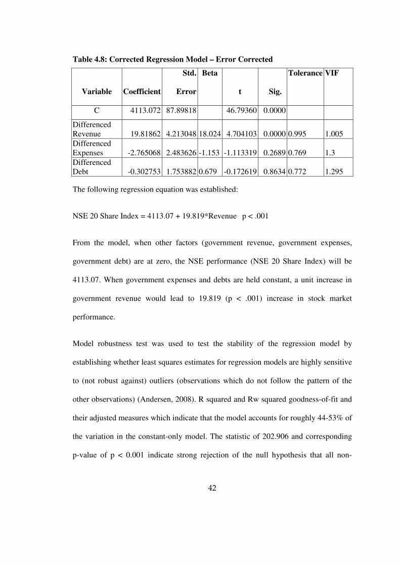
42

Table 4.8: Corrected Regression Model – Error Corrected

Variable Coefficient

Std.

Error

Beta

t Sig.

Tolerance VIF

C 4113.072 87.89818 46.79360 0.0000

Differenced Revenue 19.81862 4.213048 18.024 4.704103 0.0000 0.995 1.005

Differenced Expenses -2.765068 2.483626 -1.153 -1.113319 0.2689 0.769 1.3

Differenced Debt -0.302753 1.753882 0.679 -0.172619 0.8634 0.772 1.295

The following regression equation was established:

NSE 20 Share Index = 4113.07 + 19.819*Revenue p < .001

From the model, when other factors (government revenue, government expenses,

government debt) are at zero, the NSE performance (NSE 20 Share Index) will be

4113.07. When government expenses and debts are held constant, a unit increase in

government revenue would lead to 19.819 (p < .001) increase in stock market

performance.

Model robustness test was used to test the stability of the regression model by

establishing whether least squares estimates for regression models are highly sensitive

to (not robust against) outliers (observations which do not follow the pattern of the

other observations) (Andersen, 2008). R squared and Rw squared goodness-of-fit and

their adjusted measures which indicate that the model accounts for roughly 44-53% of

the variation in the constant-only model. The statistic of 202.906 and corresponding

p-value of p < 0.001 indicate strong rejection of the null hypothesis that all non-

43

intercept coefficients are equal to zero. Thus, as stated by Anderson, the regression is

robust and the validity of its results is not be compromised.

The regression results show that holding other factors (government expenses and

government debt) constant, a unit increase in government revenue would lead to

19.819 (p < .001) increase in NSE performance. Holding government revenue and

debt constant, a unit increase in a government expenses would lead to a 2.765

decrease in NSE performance. Afonso and Furceri (2010) found that government

investment and expenditure has sizable negative and statistically significant effect on

growth and performance of stock market. Furthermore, holding other factors

(government revenue and expenses) constant, a unit increase in government debt

would lead to a 0.3028 decrease in NSE performance. This is in line with Barro

(1979) who indicated that an increase in government borrowing raise the (short-term)

interest rate which, in turn, lower the discounted cash flow value from an asset (like a

share) and thus signals a reduction in stock market activity (aside from other adverse

effects in the general economy).

Figure 4.2 presents the graph of the model’s residuals plotted over time. The graph is

balance against 0 which signifies lack of serial correlation.

44

Figure 4.2: Residual Graph

4.5 Discussion of Research Findings

From the above analysis, the study found out that there there was a positive

correlation between NSE 20 Share Index, and Revenue (0.055) , Expenses (0.062)

and Debt (0.106). However, these positive correlations were between stock market

(NSE) performance and fiscal policy tools (government revenue, expenses and debt)

were minimal. However, the independent variables had high collinearity owing to

their correlation value between them. From the model, when other factors

(government revenue, government expenses, government debt) are at zero, the NSE

performance (NSE 20 Share Index) will be 3931.92. Holding other factors

(government expenses and government debt) constant, a unit increase in government

revenue would lead to 0.683 decrease in NSE performance

-1600

-1200

-800

-400

0

400

800

1200

1600

2007 2008 2009 2010 2011 2012

NSE_20_SHARE_INDEX Residuals

45

Holding government revenue and debt constant, a unit increase in a government

expenses would lead to a 0.575 increase in NSE performance. Furthermore, holding

other factors (government revenue and expenses) constant, a unit increase in

government debt would lead to a 0.291 increase in NSE performance. However, the

diagnostic statistics shows that the regression model was weak owing to serial

autocorrelation as the Durbin Watson value was 0.085641. The model was also weak

and insignificant owing to R-square and F-test significance values of 0.011549 and

0.733 (p > .05) respectively. Variance Inflation Factors (VIF) shows that there is high

collinearity amongst the independent variables as the VIF values were above the

critical value of 10: government revenue (139.624), government expenses (155.325).

However, government debt was not highly collinear to other independent variables as

its VIF value was 2.718. Thus, the study had to correct the regression model of

autocorrelation and collinearity problems.

From the model, when other factors (government revenue, government expenses,

government debt) are at zero, the NSE performance (NSE 20 Share Index) will be

4113.07. Holding other factors (government expenses and government debt) constant,

a unit increase in government revenue would lead to 19.819 (p < .001) increase in

NSE performance.

Holding government revenue and debt constant, a unit increase in a government

expenses would lead to a 2.765 decrease in NSE performance. Furthermore, holding

other factors (government revenue and expenses) constant, a unit increase in

government debt would lead to a 0.3028 decrease in NSE performance.

46

The diagnostic statistics shows that the regression model had a moderate strength

given r-square value of 0.254. This depicts that independent variables (government

revenue, government expenses, government debt) would cause 25.4% of the

variations in NSE performance. ANOVA statistics shows an F-test value of 9.114 at p

= p < .001. This signifies a significant linear model.

47

CHAPTER FIVE

SUMMARY, CONCLUSION AND RECOMMENDATIONS

5.1 Introduction

This chapter presents the research summary, conclusions, limitations of the study and

recommendations for further research.

5.2 Summary of Findings

The study sought to determine the relationship between fiscal policy and performance

of Nairobi Securities Exchange as measured by the NSE 20-share index. To achieve

the objective, the study employed monthly secondary data on fiscal policy variables

and the NSE 20-share index which were obtained from the CBK, KRA, KNBS and

NSE. The study regression model expressed the NSE 20-share index as a function of

the fiscal policy instruments which included government revenue, government

expenditure and government debt. The study covered a period from January 2004 to

December 2013 and data were analysed using multiple linear regression model.

The correlation matrix for the three variables shows that there are low correlations

between individual independent variables and NSE stock performance as measured by

NSE-20 share Index. However, correlation coefficients between NSE 20 share index

and the independent variables are positive showing that they move in the same

48

direction. That is, increase in government’s revenues, expenses and debt would

individually lead to improved stock performance.

Unit root test for the data revealed presence of unit root at levels by giving ADF

statistics for the three variables (NSE-20 share index, Government revenue, expenses

and debt) greater than their respective t critical values at various levels. However, this

was corrected by second order seasonal differencing. From the regression results,

government revenue (p < .001) was found to be more significant in explaining

Kenya’s stock market performance (NSE-20 share index) than Government expenses

and debt. The explanatory variables explain 22.7% of the variation in the dependent

variable. Jointly, all the variables were found to be significant as postulated by the F-

statistic (p < .001).

5.3 Conclusion

Fiscal policy has a multi-dimensional role in stock market performance. Stock prices,

not only a reflection of the developments made in the economic sector, but also

provide feedback to the government and fiscal authorities on how the economy is

fairing. They also showcase the expectations of the private sector on the future course

of key macroeconomic variables. The study established that government revenue has

a positive effect on stock market performance. Government raise revenues through

charging taxes on economic activities undertaken by its citizens reflecting a positive

economic performance as tax rate in Kenya has been consistent and constant.

Government revenue also reflects greater macroeconomic performance which makes

stock prices (stock performance) better.

49

The study concludes that Government expenditure has a positive effect on stock

market performance. Public spending reflects both microeconomic and

macroeconomic considerations. Expenditure as outlined in the state budget reflects

the economic scale, balance and direction of a country. Increasing government

spending is the main tool in expansionary fiscal policy. Government can finance its

spending by either taxation or issuing bonds. The result normally helps to lift stock

prices. Besides, government spending change creates more immediate impact on

domestic economic growth and consequently benefits the stock market.

The study findings showed that government debt has low positive effect on stock

market performance and negative cumulative effect on the same. Kenya borrows

through issuance of bonds and direct borrowing from foreign governments and

supranational organizations like World Bank, International Monetary Fund (IMF),

Africa Development Bank (ADB) et cetera. The interaction two sources of borrowing

contributes to the growth or redundancy of an economy that seeks to outlive any

impulses that slow it down. The fiscal policy is expected to influence the goods

market while the monetary policy is expected to utilize its effect on asset markets.

Without imposing the risk of inflation owing to interest rates on debt, debts helps

cover for deficits in expected expenditure versus revenue which leads to infrastructure

development and economic stimulus plan. This leads to economic growth and better

firms’ performance which raises their market value and stock performance. Besides,

investors are inclined to allocate capital back and forth between bond and stocks

facing different risks.

50

5.4 Recommendations

From the research findings, it is evident that government fiscal policies play an

important role in explaining variations on stock market performance. From the

analysis made in the previous chapter, various recommendations can be made. There

is need for users of stock indices to understand their computations and constituent

counters in any given stock exchange. For example, the NSE 20 share index appears

to be more significant in explaining variations in market capitalization which could be

attributed to the fact that the 20 counters that constituent the index account for over

80% of the total turnover at the exchange on any given day. This has the likelihood to

present a strong co-movement between the market capitalization and the NSE 20

share index as opposed to NASI which involves all the counters including the least

traded. Inclusion of the least traded counters in the computation of the index results in

smoothening out of the variations or the volatility of the stock market. As a result,

NSE needs to address that selection bias and related anomalies in the indices.

5.5 Limitations of the Study

A number of limitations could be pointed out for this study. Firstly, this descriptive

and correlational study relied on secondary data which had already been compiled by

the KNBS, KRA, CBK and NSE. Data was used as they were obtained from the

sources and the researcher had no means of verifying for the validity of the data

which were assumed to be accurate for the purpose of this study. The study results are

therefore subject to the validity of the data used.

51

Secondly, the study was conducted in Kenya and its results may not be generally

applicable in other countries whose economic, fiscal policy targets and stock market

development conditions may be different from those of Kenya.

Finally, the study used the ordinary least square regression method of analysis which

may have its own weaknesses compared to other methods which may limit the general

applicability of the study results.

5.6 Suggestions for Further Research

The findings of this study are only confined to the relationship between stock market

performance and government fiscal policies. Based on these findings further research

can be done to determine that relationship between the variables under different

governments as presidents determine the fiscal policies of their governments.

This study examined the relationship and the extent of the relationship of the variables

under study for a period of ten years only. A further study can be done to forecast

whether such relationship will hold in longer period. In addition, effects of equity

turnover on stock market performance can also be studied and its impact on the

indices established.

52

REFERENCES

Afonso, A. & Sousa, R. M. (2011). What Are The Effects of Fiscal Policy on Asset

Markets? Economic Modeling, 28(4), 1871-1890.

António, A., Furceri, D. & Pedro G. (2010). Sovereign credit ratings and financial

markets linkages: application to European data, Working Papers Department

of Economics.

Ali, S.M. & Hasan, M.A. (2003). Is the Canadian stock market efficient with respect

to fiscal policy? Some vector autoregression results, Journal of Economics

and Business 45(1), 45-59.

Ambunya, P. L. (2012). The Relationship between Exchange rate movement and

stock market returns volatility at the Nairobi Securities Exchange.

Unpublished MBA project, University of Nairobi.

Andersen, R. (2008). Modern Methods for Robust Regression. Sage University Paper

Series on Quantitative Applications in the Social Sciences, 07-152.

Arin, K. P., Mamun, A. & Purushothman, N. (2009). The effects of Tax Policy on

Financial markets: G3 Evidence. Review of Financial Economics, 18(4), 33-

46.

Babak, M.D. (2012). The Misleading Value of Measured Correlation. Wilmott, (1):

64–73

Baharumshah, A. Z., Masih, A. M., & Azali, M. (2002). The Stock market and The

Ringgit Exchange Rate: A Note. Japan and The World Economy, 14, 471-486.

Barro, R.J. (1974). Are government bonds net wealth? Journal of Political Economy.

82, 1095-1117`

53

Barro, R.J. (1979). On the determination of public debt, Journal of Political Economy.

87 (1), 940-971

Belle, G.B. (2008). Statistical rules of thumb (2nd ed.). Hoboken, N.J: Wiley.

Bernanke, B. S. & Kuttner, K. N. (2005). What explains the stock market’s reaction to

federal reserve policy? Journal of Finance, 60(3), 1221–1258.

Blancahrd, O & F Giavazzi, (2003). Macroeconomics Effects of Regulation and

Deregulation on Goods and Labour markets, Quarterly Journal of Economics:

879-906

Blanchard, O. J. & Perotti, R. (1999). An empirical characterization of the dynamic

effects of changes in government spending and taxes on output. NBER

Working Paper no. W7269.

Blanchard, O. J. (1981). Output, the stock market and interest rates, American

Economic Review 71, 132-43.

Bordo, M.D. (2009). Inflation, Monetary Policy and Stock Market Conditions:

Quantitative Evidence from Hybrid Latent –Variable VAR, Federal Reserve

Bank of St Louis, Working Paper Series.

Calderon, C. & Serven, L. (2003a). The Output Cost of Latin America’s Infrastructure

Gap. In: Easterly, W. Serven, L,eds, The Limits of stabilization:

Infrastructure, Public Deficits and growth in Latin America, Stanford

University Press and the World Bank 95-118.

Central Bank of Kenya (CBK) (2014). Government Finance Statistics. Accessed May

30th, 2014, https://www.centralbank.go.ke/index.php/balance-of-payment

statistics/government-finance-statistics.

54

Darrat, A. F. (1987). Money and stock prices in West Germany and the UK: is the

stock market efficient? Quarterly Journal of Business and Economics 26: 32-

45.

Darrat, T. & Brocato, J. (1994). Stock market efficiency and the federal budget

deficit: another anomaly, The Financial Review 29, 49-75.

Devarajan, T., Prychitko, D. L., Nogueira, M. & Tafri, F. H. (1996). Political

Economy of Public Capital Formation in Japan, Public Policy Review. 4 77-

110.

Dufour J. M. & Tessier, D. (2006). Short-Run and Long-Run Causality between

Monetary Policy Variables and Stock Prices, Working Papers 06-39.

Fama, E.F., & Schwert, G.W. (1977). Asset returns and inflation, Journal of

Financial Economics 5, 115-46.

Fama, E. (1965a). The behavior of stock market prices. Journal of Business 38, 34–

105.

Fama, E. (1965b). Random walks in stock market prices. Financial Analysts Journal

21, 55–9.

Fama, E. (1970). Efficient capital markets: a review of theory and empirical work.

Journal of Finance 25, 383–417.

Fama, E. & Blume, M. (1966). Filter rules and stock market trading profits. Journal of

Business 39, 226–41.

Fama, E. & French, K.(1988). Permanent and temporary components of stock prices.

Journal of Political Economy 96, 246–73.

55

Filis, G. (2010). Macro economy, Stock market and Oil Prices: Do meaningful

relationships exist Among Their Cyclical Fluctuations? Energy Economics,

32, 877-886.

French, K. & Roll, R. (1986). Stock return variances: the arrival of information and

the reaction of traders. Journal of Financial Economics 17, 5–26.

Fuente, A. (1997). Fiscal Policy and Growth in the OECD. Discussion Paper Series

No 1755. Centre for economic Policy Research: London, UK.

Godspeed, I. (2008). Introduction to financial markets, South African Institute of

Financial Markets.

Gordon, M. J. (1962). The Investment, Financing and Valuation of the Corporation.

Irwin: Homewood ILL.

Government of Kenya, (June 2011). Medium- Term Budget Strategy Paper, 2009/10-

2011/12.

Greene, W. H. (2002). Econometric Analysis, Fifth ed. New Jersey: Prentice Hall.

Greenspan, A. (2002). Economic Volatility, Remarks made at a Symposium

Sponsored by the Federal Reserve Bank of Kansas City, Jackson Hole.

Gujarati, D. (2007). Basic Econometrics. New Delhi: Tata McGraw-Hill.

Heyne, P. T., Boettke, P. J. & Prychitko, D. L. (2002). The Economic Way of Thinking

(10th ed). Prentice Hall: Lariman publishers.

Hondroyiannis, G. & Papapetrou, E. (2001). Macroeconomic influences on the stock

market, Journal of Economics and Finance, 25(1): 33-49.

Hördahl, P. & King, M. R. (2008). Developments in Repo Markets During the

Financial Turmoil, BIS Quarterly Review. 4: 37-53.

56

Hosseini, S. M., Ahmad, Z. & Lai, Y. W. (2011). The Role of Macroeconomics

Variables on Stock Market Index in China and India. International Journal of

Economics and Finance, 3(6), 233-243.

Ibrahim, M. H., & Wan Yusoff, W. S. (2001). Macroeconomics Variables, Exchange

rate and Stock Price: A Malaysian Perspective. IIUM Journal of Economics

and management, 9(2), 141-163.

Imran, A. (2009). Causal relationship between macroeconomic indicators and stock

exchange prices in Pakistan, The African Journal of Business Management.

4,312.

Jarque, C.M. & Bera, A.K. (1980). Efficient tests for normality, homoscedasticity and

serial independence of regression residuals. Economics Letters 6 (3): 255–259.

Jensen, G. R. & Johnson, R. R. (1995). Discount Rate Changes and Security Returns

in the U.S., 1962-1991. Journal of Banking and Finance. 19, 79-95.

Jensen, G. R. (1996). Business Conditions, Monetary Policy, and Expected Security

Returns, Journal of Financial Economics, 40, 213–37.

Kariuki, D. K. (2003). Determinants of Fixed Capital Formation in Kenya.

Unpublished M.A Research paper, Makerere University, Kampala, Uganda.

Kenya National Bureau of Statistics (KNBS) (2014). Kenya Statistics. Nairobi:

KNBS.

Keynes, J.M. (1936). The General Theory of Employment, Interest, and Money,

London: Macmillan.

Kim, K.H. (2003). Dollar Exchange Rate and stock Price: Evidence From multivariate

Co-integration and Error Correction model. Review of Financial Economics,

12(3), 301-313.

57

Kimani, D.K., & Mutuku, C.M. (2013). Inflation Dynamics On The Overall Stock

Market Performance: The Case of Nairobi Securities Exchange in Kenya.

Economics and Finance Review Vol. 2(11) pp. 01 – 11.

Kirira, N. (2009). Public Finance under Kenya’s new Constitution. Working Paper

No 5.

Kondoh, H. (2008). Political Economy of Public Capital Formation in Japan, Public

Policy Review. 4 77-110.

Laopodis, N. T. (2006). Dynamic linkages among the stock market, inflation,

monetary policy and real activity, The Financial Review 41(4).

Laopodis, N. T. (2009). Fiscal Policy and Stock Market Efficiency: Evidence For The

United State. The Quarterly Review of Economics and Finance, 49(2), 633-

650.

Larch, M., & Nogueira, M. (2009). Fiscal Policy Making in the European Union - An

Assessment of Current Practice and Challenges. London: Routledge.

Lee, B. D. (1992). Causal relations among stock returns, interest rates, inflation, and

real activity, Journal of Finance 42(4), 1591-1603.

Lee, U. (1997). Stock market and macroeconomic policies: new evidence from Pacific

Basin countries, Multinational Finance Journal 1(2), 273-289.

Makkonen, L., Pajari, M. & Tikanmäki, M. (2013). Closure to Problems in the

Extreme Value Analysis. Structural Safety 40 (1), 65–67,

Maysami, R. C. & Koh, T. S. (2000). A Vector Error Correction Model of The

Singapore stock Market, International Review of Economics and Finance, 9,

79-96.

58

Mishkin, F. S. (1996). The Channels of Monetary Transmission: Lessons for

Monetary Policy, NBER Working Papers 5464, Cambridge: National Bureau

of Economic Research.

Mishkin, F. S. (2000). International Experiences with Different Monetary Policy

Regimes, NBER Working Papers 7044, National Bureau of Economic

Research, Cambridge.

Mishkin, F. S. (2007). The Economics of Money, Banking and Financial Markets, 8th

Edition, New York: Pearson Addison Wesley.

Mongeri, O. (2011). The impact of foreign exchange rates and foreign exchange

reserves on the performance of Nairobi stock exchange share index.

Unpublished MBA project, University of Nairobi.

Muchiri, H. G. (2012). The impact of macroeconomic variables on the performance of

the Nairobi securities exchange. Unpublished MBA project, University of

Nairobi.

Muiru, J. S (1977). The Effectiveness Of Kenya's Monetary Policy During The

Period 1967 -1976. Unpublished MBA project, University of Nairobi.

Mugenda, M.O., & Mugenda, G.A. (2003). Research Methods: Qualitative and

Quantitative Approaches. Nairobi: ACTS Press

Mutoko, R. K. (2006). Analysing effect of treasury bill rates on stock market returns

using GARCH. Unpublished MBA Project, University of Nairobi.

Mwanza, D.K. (2012). The relationship between monetary policy and Performance of

the Nairobi securities exchange. Unpublished MBA Project, University of

Nairobi.

59

Ngigi, R. W. (2000). The impact of fiscal and monetary policies on stock market

performance in Kenya: an empirical analysis. Unpublished MBA Project,

University of Nairobi.

Njenga, E.N. (2012). Relationship between Fiscal Policy and Public Investment in

Kenya. Unpublished MBA Project, University of Nairobi, Kenya.

Nyamute, M. (1998). The Relationship between Stock Prices and Exchange Rates,

Interest Rates, Money Supply and Inflation. Unpublished MBA Project,

University of Nairobi.

Pilbeam, K. (1998). Finance and Financial Market, Hampshire Palgrave: Basingtoke.

Rahman, A., Sidek, N. Z., & Tafri, F. H. (2009). Macroeconomics Determinants of

Malaysia Stock Market. African Journal of Business Management, 3(3), 95-

106.

Richards, A., & How, J. (2006). Robust stable model predictive control with

constraint tightening. Proceedings of the American Control Conference,

Washington, June 25, 2006.

Rogalski, R., & J. Vinso, (1977). Stock returns, money supply and the direction of

causality, Journal of Finance 32, 1017-1-30.

Roubini, N. & Sachs, J. (1989). Political Economic Determinants of Budget Deficits

in the Industrial Economies. NBER Working Paper No. 2682, European

Economic Review, 1989.

Serven, L., & Soliman A. (1993). Private Investment and Macroeconomic

Adjustment: A survey. In Lius Serven amd Andres Soliman, Striving for

Growth After Adjustment, Washington D.C: World Bank.

60

Shah, A. (1984). Crowding out, capital accumulation, the stock market, and money-

financed fiscal policy, Journal of Money, Credit, and Banking 16(part 1), 461-

473.

Siele, W. (2009). The Relationship between Selected Macroeconomic Variables and

NSE 20-share index, Unpublished MBA dissertation, University of Nairobi.

Sifunjo, K. (1999). The causal relationship between exchange rates and stock prices in

Kenya. Unpublished MBA Project, University of Nairobi.

Siklos, P., & Kwok, B. (1999). Stock Returns and Inflation: A New Test of

Competing Hypotheses, Applied Financial Economics 9, 567-81.

Silvia, J. & Iqbal, A. (2011). Monetary Policy, Fiscal Policy, and Confidence.

International Journal of Economics and Finance, 3(4), 22-35.

Simiyu, M. (1992). Measuring Market Performance of the NSE. Unpublished MBA

Project, University of Nairobi.

Smith, E. L. (1925). Common Stocks as long term investments, New York:

Macmillan.

Steven, M. S. (2003). Economics: Principles in action. Pearson Prentice Hall: Upper

Saddle River.

Studenmund, A.H. (2006). Using Econometrics: A practical guide, 5th Edition.

London: Pearson International Edition.

Thorbecke, W. (1997). On stock market returns and monetary policy, Journal of

Finance 52(2), 635-654.

Tobin, J. (1969). A General Equilibrium Approach to Monetary Theory, Journal of

Money, Credit and Banking, 1, 15-29.

61

Veganzones, V. (2005). How to Boost Private Investment in the MENA Countries.

The Role of Economic Reforms. 4: 381.

Garcia, V. F. (1999). Macroeconomic determinants of stock market development,

Journal of Applied Economics, 2, 23.

Yartey, C. A. (2008). The determinants of stock market development in emerging

economies: Is South Africa different? IMF working paper.

Wongbangpo, P. & Sharma, S. C. (2002). Stock Market and macroeconomics

Fundamental Dynamic Interactions: ASEAN-5 Countries. Journal of Asian

Economics, 13,27-51.

World Bank, (2005). Public Investment and Fiscal Policy- Lessons from the Pilot

Country Studies,” The World Bank, Washington , D.C

www.cbk.

www.knbs.or.ke

www.kra.go.ke

www.mystocks.co.ke

www.nse.go.ke.

62

APPENDICES

Appendix I: Multiple Line Graphs

63

Appendix II: Q-Q Plots

64

Appendix III: Differenced Variables

-1000

-800

-600

-400

-200

0

200

400

600

2005 20 06 2007 2008 2009 20 10 2011 2012 2013

D_NSE_20_SHARE_INDEX

200

300

400

500

600

700

800

900

1000

1100

2005 2006 2007 20 08 2009 2010 2011 20 12 2013

DEBT

0

200

400

600

800

1000

1200

2005 20 06 2007 2008 2009 20 10 2011 2012 2013

EXPENSES_KSH_BN

0

1

2

3

4

5

6

7

8

2005 20 06 2007 2008 2009 20 10 2011 20 12 2013

GDP

- .04

- .02

.00

.02

.04

.06

.08

.10

2005 2006 2007 20 08 2009 2010 2011 20 12 2013

LD_DEBT

- .04

- .02

.00

.02

.04

.06

.08

.10

2005 20 06 2007 2008 2009 20 10 2011 2012 2013

LD_DEBT_1

-4

-3

-2

-1

0

1

2

2005 2006 2007 20 08 2009 2010 2011 20 12 2013

LD_EXPENSES_KSH_BN

-4

-3

-2

-1

0

1

2

2005 20 06 2007 2008 2009 20 10 2011 2012 2013

LD_EXPENSES_KSH_BN_1

-3

-2

-1

0

1

2005 20 06 2007 2008 2009 20 10 2011 20 12 2013

LD_REVENUE_KSH_BN

-3

-2

-1

0

1

2005 2006 2007 20 08 2009 2010 2011 20 12 2013

LD_REVENUE_KSH_BN_1

38000

38500

39000

39500

40000

40500

41000

41500

2005 20 06 2007 2008 2009 20 10 2011 2012 2013

MONTH

2400

2800

3200

3600

4000

4400

4800

5200

5600

6000

2005 2006 2007 20 08 2009 2010 2011 20 12 2013

NSE_20_SHARE_INDEX

0

10 0

20 0

30 0

40 0

50 0

60 0

70 0

80 0

90 0

2005 2006 20 07 2008 2009 2010 20 11 2012 20 13

REVENUE_KSH_BN

0

40

80

120

160

200

20 05 2006 2007 2008 20 09 2010 2011 2012 20 13

SD_DEBT

-40

0

40

80

120

160

200

2005 20 06 2007 2008 2009 20 10 2011 20 12 2013

SD_EXPENSES_KSH_BN

-20

0

20

40

60

80

10 0

12 0

20 05 2006 20 07 2008 20 09 2010 20 11 2012 2013

SD_REVENUE_KSH_BN

-100

-50

0

50

100

150

2005 20 06 2007 2008 2009 20 10 2011 2012 2013

SD_SD_DEBT

-120

-80

-40

0

40

80

120

2005 2006 20 07 2008 2009 2010 20 11 2012 20 13

SD_SD_EXPENSES_KSH_BN

-80

-60

-40

-20

0

20

40

60

80

2005 20 06 2007 2008 2009 20 10 2011 2012 2013

SD_SD_REVENUE_KSH_BN

65

Appendix IV: Study Data Month Revenue

Ksh bn

Expenses

Ksh bn

Debt

Ksh bn

GDP NSE 20 Share

index

Jan-04 130.10 146.01 291.22 89,200 3,961

Feb-04 148.44 166.64 292.23 92,301 3,963

Mar-04 169.70 189.42 296.33 91,920 3,965

Apr-04 195.71 212.75 307.16 80,139 3,968

May-04 216.21 231.63 304.98 91,005 3,970

Jun-04 254.68 282.19 315.57 86,271 3,972

Jul-04 16.82 20.44 303.46 100,186 2,708

Aug-04 37.15 42.38 301.68 85,157 2,709

Sep-04 60.64 65.94 299.75 93,192 2,671

Oct-04 85.63 88.78 301.54 91,783 2,830

Nov-04 108.54 113.26 302.54 103,491 2,918

Dec-04 144.56 133.64 295.37 98,462 2,946

Jan-05 169.76 154.53 291.22 94,195 3,094

Feb-05 190.56 172.95 292.23 91,920 3,213

Mar-05 219.10 202.30 296.33 93,762 3,209

Apr-05 232.81 229.95 307.16 89,103 3,228

May-05 254.18 260.79 304.98 95,340 3,505

Jun-05 304.70 303.40 315.57 92,606 3,972

Jul-05 16.30 24.70 324.03 103,589 3,982

Aug-05 37.30 53.20 325.38 97,920 3,939

Sep-05 68.70 86.20 328.80 101,010 3,833

Oct-05 95.10 117.80 332.73 99,281 3,939

Nov-05 116.30 141.30 333.50 109,910 3,974

Dec-05 148.30 179.20 335.00 104,333 3,973

Jan-06 183.00 209.80 333.95 102,004 4,172

Feb-06 203.90 235.30 338.61 93,521 4,057

Mar-06 229.90 268.50 346.06 99,396 4,102

Apr-06 253.10 292.60 348.22 104,924 4,025

May-06 295.93 337.04 349.49 91,625 4,349

Jun-06 327.80 383.00 357.84 98,379 4,260

Jul-06 21.70 24.70 364.84 103,480 4,259

Aug-06 47.90 59.40 367.96 112,745 4,486

Sep-06 77.60 94.30 371.59 109,289 4,880

Oct-06 104.70 124.40 375.52 100,457 5,314

Nov-06 128.66 157.48 381.30 115,952 5,615

Dec-06 170.16 194.39 385.10 109,422 5,646

Jan-07 195.32 219.73 378.10 108,341 5,774

66

Month Revenue

Ksh bn

Expenses

Ksh bn

Debt

Ksh bn

GDP NSE 20 Share

index

Feb-07 221.74 255.44 385.80 102,683 5,387

Mar-07 256.71 284.20 386.29 106,362 5,134

Apr-07 305.21 334.50 390.49 110,634 5,199

May-07 331.21 368.65 390.30 102,850 5,002

Jun-07 383.59 405.20 404.69 106,492 5,147

Jul-07 34.20 29.30 410.20 124,284 5,340

Aug-07 66.00 69.60 415.90 109,230 5,372

Sep-07 97.96 94.06 426.80 116,190 5,146

Oct-07 135.14 143.49 418.50 128,361 4,971

Nov-07 168.95 188.63 426.02 99,291 5,215

Dec-07 211.95 239.64 438.20 116,581 5,445

Jan-08 253.90 284.50 432.18 112,793 4,713

Feb-08 282.67 314.95 434.55 100,257 5,072

Mar-08 322.58 341.79 444.75 107,754 4,843

Apr-08 362.36 393.93 437.94 105,845 5,336

May-08 402.67 449.75 442.68 113,826 5,176

Jun-08 457.67 534.84 430.61 109,064 5,186

Jul-08 33.20 29.24 428.22 115,805 4,868

Aug-08 68.03 74.36 433.56 124,843 4,649

Sep-08 111.70 123.60 449.25 119,272 4,180

Oct-08 150.10 179.20 454.70 123,004 3,387

Nov-08 184.15 210.51 451.39 110,458 3,341

Dec-08 236.60 241.70 456.20 116,457 3,521

Jan-09 277.42 301.54 454.27 109,341 3,199

Feb-09 318.85 359.38 479.08 116,900 2,475

Mar-09 361.27 406.94 474.89 113,755 2,805

Apr-09 407.21 465.12 497.58 111,903 2,800

May-09 449.64 515.70 489.34 109,585 2,853

Jun-09 511.35 621.91 518.51 110,091 3,295

Jul-09 40.08 44.77 530.53 118,943 3,273

Aug-09 74.82 98.61 547.21 120,115 3,103

Sep-09 128.90 159.30 550.69 119,890 3,005

Oct-09 170.83 210.69 567.13 118,992 3,084

Nov-09 208.56 246.75 562.93 122,883 3,190

Dec-09 266.08 296.13 588.97 120,541 3,247

Jan-10 311.97 372.03 580.70 117,805 3,565

Feb-10 350.66 440.03 608.00 120,345 3,629

Mar-10 394.40 490.64 639.10 119,047 4,073

67

Month Revenue

Ksh bn

Expenses

Ksh bn

Debt

Ksh bn

GDP NSE 20 Share

index

Apr-10 455.12 561.39 653.60 113,800 4,233

May-10 502.03 644.54 650.30 117,402 4,242

Jun-10 560.79 718.65 659.61 115,899 4,339

Jul-10 38.59 35.91 667.80 124,500 4,439

Aug-10 83.00 112.20 698.05 131,045 4,455

Sep-10 142.43 178.61 704.70 127,244 4,630

Oct-10 193.09 243.14 696.13 122,000 4,660

Nov-10 243.16 303.78 711.45 135,820 4,395

Dec-10 309.23 368.99 720.33 127,925 4,433

Jan-11 362.57 432.16 726.32 130,001 4,465

Feb-11 408.80 489.40 746.86 109,551 4,240

Mar-11 463.90 560.00 758.66 121,528 3,887

Apr-11 525.70 631.10 735.50 126,990 4,029

May-11 584.80 687.60 746.60 116,045 4,078

Jun-11 679.50 817.10 764.22 121,833 3,968

Jul-11 42.70 43.72 781.71 140,782 3,738

Aug-11 91.28 95.88 776.85 129,500 3,465

Sep-11 159.25 179.63 764.27 135,484 3,284

Oct-11 210.31 248.30 795.21 129,745 3,507

Nov-11 265.47 320.58 803.89 139,004 3,155

Dec-11 345.66 430.93 800.68 134,460 3,205

Jan-12 398.16 512.65 809.28 131,004 3,224

Feb-12 450.53 586.55 877.29 124,426 3,304

Mar-12 510.89 663.82 887.87 126,503 3,367

Apr-12 585.16 740.82 896.04 123,950 3,547

May-12 656.32 817.43 889.06 130,451 3,651

Jun-12 734.43 915.89 858.83 127,276 3,704

Jul-12 46.27 50.03 872.16 132,958 3,832

Aug-12 103.88 146.19 901.85 150,281 3,866

Sep-12 173.32 232.29 922.20 141,621 3,972

Oct-12 233.02 308.06 929.32 150,683 4,147

Nov-12 304.41 405.53 958.44 129,002 4,084

Dec-12 387.89 506.41 971.27 141,294 4,133

Jan-13 454.06 589.55 977.90 133,804 4,417

Feb-13 514.26 664.32 943.80 131,893 4,519

Mar-13 577.30 776.10 981.90 132,940 4,861

Apr-13 675.70 882.10 1,065.60 128,504 4,765

May-13 758.30 995.20 1,074.80 135,904 5,007

68

Month Revenue

Ksh bn

Expenses

Ksh bn

Debt

Ksh bn

GDP NSE 20 Share

index

Jun-13 851.19 1,100.83 1,050.56 132,777 4,598

Jul-13 58.60 49.70 1,078.60 142,804 4,788

Aug-13 128.42 150.58 1,116.68 154,802 4,698

Sep-13 210.23 269.87 1,168.23 147,800 4,793

Oct-13 286.22 357.20 1,174.78 135,258 4,993

Nov-13 363.59 473.98 1,170.05 140,847 5,101

Dec-13 468.97 574.21 1,189.18 138,977 4,927

Source: CBK (2014), KNBS (2014)