Replication of: “Meta-analysis of the effect of fiscal policies on long-run growth”

(European Journal of Political Economy, 2004)

by

Nurul Sidek and W. Robert Reed†

Department of Economics and Finance University of Canterbury

Christchurch, New Zealand

Abstract

This study replicates the empirical findings of Nijkamp & Poot (2004), henceforth N&P, and performs a variety of robustness checks. Using a sample of fiscal policy studies published between 1983-1998, N&P concluded that certain types of fiscal policies were more likely to match prior beliefs about their impact on economic growth than others. N&P also identified study attributes that impacted the likelihood of confirmation. We first demonstrate that we are able to exactly replicate their findings. We then attempt an alternative replication, returning to the original studies, and independently categorizing them using N&P’s general classification scheme. We also investigate the implications of a number of methodological improvements on their analysis. Our replication efforts produce results that are qualitatively similar to N&P, though very few of our results are statistically significant. We use the lessons learned from this replication effort to suggest directions for future meta-analysis studies on the subject of fiscal policy and economic growth.

11 September 2013

†Corresponding author: W. Robert Reed, Private Bag 4800, Christchurch 8140, New Zealand. Phone: +64-3-364-2846; Email: bob.reed@canterbury.ac.nz Acknowledgements: We acknowledge helpful comments from participants at the Meta-Analysis in Economic Research Network conference in London, UK, September 5-7. We are especially grateful to Peter Nijkamp and Jacques Poot for making all of their data available to us. Jacques Poot went far beyond the call of duty in answering our many questions. More than that, we appreciate his openness to allowing their study to be subject to critical analysis. Openness and integrity are the bases by which science advances.

1

I. INTRODUCTION Meta-analyses are studies that analyze empirical results from other studies. They attempt to

relate a specific empirical finding, such as an estimated elasticity or treatment effect size, to

characteristics of the studies themselves. Characteristics can include the particular type of

estimation methodology that was employed (e.g., OLS, FGLS, 2SLS, etc.); the type of data

that was used (time series, cross-sectional, panel data, etc.); the control variables included in

the specification; or some other feature that the meta-analysis researcher believes can affect

the results of empirical analysis. Meta-analyses are useful for a number of reasons. Firstly,

by combining results from numerous studies, they can lead to more precise estimates of the

respective elasticity, treatment effect, or other estimated outcome. Secondly, they can help to

explain why different studies produce different estimates. This, in turn, can lead to improved

estimation methodologies and better estimates.

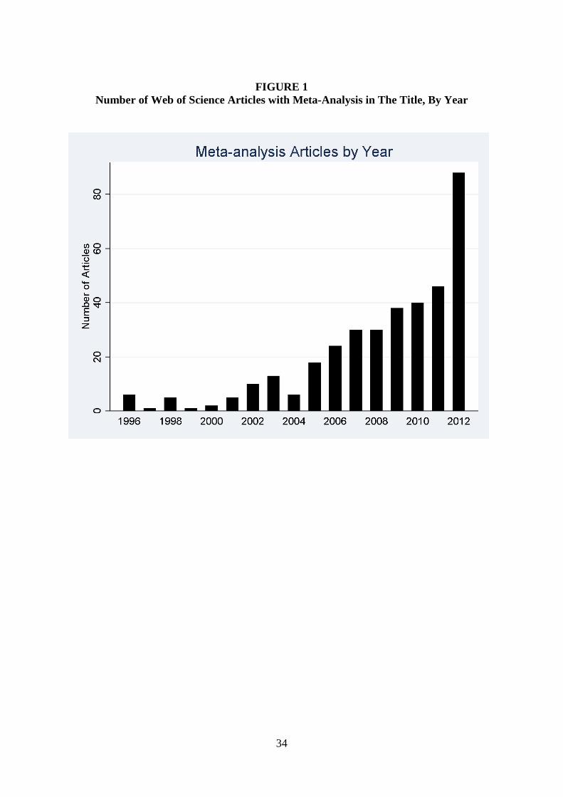
The use of meta-analysis in economics has grown explosively in recent years.

FIGURE 1 shows the growth in the number of economics articles listed by Web of Science

that include the word “Meta-analysis” in the title. There were 6 such studies published in

1996. In 2012, there were 88. While there are some generally accepted concepts that are

common to meta-analyses (e.g., fixed versus random effect estimates), there is still much

heterogeneity across studies. “Best practice” is still being worked out (Ringquist, 2013;

Stanley et al., 2013). Key components of a meta-analysis include: (i) determination of the

“dependent variable” (e.g., nominal size of elasticity/treatment effect, statistical significance

of the treatment variable, etc.); (ii) selection of research studies to analyze; (iii) identification

of study characteristics to investigate; and (iv) decision about the most appropriate

procedure(s) for estimating the relationship between the dependent variable and study

characteristics. A key element of the last item is whether to weight individual observations

2

and, if so, which weighting mechanism to apply. It should be noted that there is an important

element of subjectivity to many of these issues.

Much remains to be learned about the robustness of meta-analyses to alternative

approaches. This study aims to contribute to this subject. We replicate the study “Meta-

analysis of the effect of fiscal policies on long-run growth” by Nijkamp & Poot (2004). We

choose this study for two reasons. First, it addresses an important topic. The relationship

between fiscal policy and economic growth is highly debated in both academic and policy-

making circles. Second, the paper is influential. It has been cited 35 times in Scopus and 190

times in Google Scholar as of July 2013.

N&P analyzed 123 observations from 93 studies. Our replication uses the same

classification categories employed by N&P to determine whether subjectivity in cataloguing

the studies has an impact on the outcome of the meta-analysis. We also check for robustness

of N&P’s results to a number of alternative estimation methodologies.

Our analysis proceeds as follows. Section II describes the original N&P study and

identifies four key findings from that study. Section III reports the results of two replication

efforts. The first approach uses N&P’s data to check the reproducibility of their published

findings. The second approach implements an alternative application of N&P’s general

classification scheme. This section also identifies a number of important empirical and

conceptual issues. Section IV checks the robustness of N&P key findings to alternative

empirical methodologies. Section V summarizes our results and attempts to draw some

lessons from our research for future meta-analyses.

II. DESCRIPTION OF NIJKAMP & POOT (2004)

N&P examine 93 studies published between 1983-1998 that reported on the empirical

relationship between economic growth and one of five types of fiscal policies: (i) government

consumption, (ii) tax rates, (iii) defence, (iv) education expenditures, and (v) public

3

infrastructure.1 All of the studies were refereed journal articles except a textbook by Barro

(1997) and a chapter in an edited book by Dunne (1996). Usually, one empirical outcome

was recorded for each study, though some studies reported estimates for more than one type

of fiscal policy. N&P’s full sample comprise 123 observations.

The “dependent variable” in N&P’s analysis is a categorical variable that reports

whether a study supported the “conventional belief” regarding how a given fiscal policy

affected economic growth. With respect to government investment in education and

infrastructure, the “conventional prior belief” is that these expenditures are beneficial for

economic growth. Government consumption/size, taxes, and defence spending are posited to

be harmful to economic growth.

N&P categorize studies as either demonstrating a “conclusively positive effect,” a

“conclusively negative effect,” or having an “inconclusive result” depending on the reported

relationship between the respective fiscal policy and economic growth. In this, they do not

use their own judgment, but rely on the “personal assessment of article authors(s)” as

expressed in the study (N&P, page 93). These results are then further categorized as

“supporting,” “rejecting,” or “inconclusive” depending on whether the study’s conclusions

are in agreement with the conventional prior belief. N&P include many different types of

studies in their analysis: cross-sectional studies, panel data studies, time series studies, VAR

models (e.g., that test for Granger causality), Vector Error Correction models, CGE studies,

some review articles, and even another meta-analysis.

N&P use three empirical procedures in their meta-analysis. First, for each fiscal

policy, they construct 95% confidence intervals around the proportion of observations that

support the conventional prior. Second, they pool all the observations and then test for

significant differences in the proportion of studies supporting the prior across various pairs of

1 These studies were previously reviewed narratively in Poot (2000).

4

study characteristics (e.g., between studies that estimate conventional growth equations and

other studies; between studies published in highly ranked journals and other studies; etc.).

Lastly, they use “rough set” analysis to link study attributes to study outcomes (Pawlak,

1982; 1992). Our analysis focuses on their first two procedures.

A total of nine characteristics are reported for each study:

1. Type of fiscal policy investigated: government consumption (C), tax rates (T),defence (D), education expenditures (E), and public infrastructure (I)

2. Year of publication

3. Year of earliest observation

4. Year of most recent observation

5. Number of observations used in the study

6. Type of geographical area: (i) country or (ii) regions (e.g., states within a country)

7. Level of development of region or country: (i) developed, (ii) less developed, or (iii) mixed

8. Rank of journal that the article was published in: One of the three tiers identified in

Towe and Wright (1995), or “unranked.” 9. Type of data: (i) cross-sectional, (ii) panel data, (iii) time series, or (iv) other.

Amongst cross-sectional and panel data regression observations, N&P identified those that

were “conventional growth studies,” defined as “linear regression models with the growth in

real national output or income as the dependent variable.” Conventional growth studies were

yet further categorized according to whether they controlled for (i) initial income, (ii)

population or labour force growth, and/or (iii) investment or savings.

In their conclusion, N&P discuss a large number of findings. Our replication and

robustness analysis focuses on four findings for which the statistical evidence is strongest.

These are reported in TABLE 1.

5

III. REPLICATION OF NIJKAMP & POOT (2004)

Replication - Part I. With the exception of some data on research methodology, all of the

study attributes analysed by N&P are available in Table 2 of their paper. Column 1 of

TABLE 2 identifies a subset of the study attributes, along with the number of observations

that N&P assign to each category. Column 2 is our replication of N&P based on the data

reported in their paper, along with additional information provided by Jacques Poot.2 We are

able to exactly replicate their data, with one minor exception: We find one less regression

model with panel data. None of the main findings are affected by this discrepancy. A more

complete set of replication results are reported in the Appendix.

Replication – Part II. We also undertook a less mechanistic replication of their work

by revisiting the original 93 papers/123 observations used in N&P’s study. Using the same

classification scheme that N&P employed, we read each of the papers and made our own

judgment about how to categorize them. In the course of doing this, we discovered that there

are many issues in categorizing studies that introduce a potentially large component of

subjectivity into the meta-analysis procedure. In this section, we highlight some of the issues

we encountered in this exercise, along with a major change that we made to their procedure.

N&P classified study outcomes as demonstrating either a “conclusively positive

effect,” a “conclusively negative effect,” or an “inconclusive result” depending on whether

the study reported a positive, negative, or inconclusive relationship between the given fiscal

policy and economic growth. As noted above, N&P did not use their own criteria/judgment

for classifying outcomes. Instead, they interpreted summary statements from the studies

themselves to make this determination.

A problem with this approach is that different authors may apply different standards

in interpreting their findings. The major change we made to N&P’s procedure is that we use

2 Jacques Poot graciously supplied us with the remaining data to enable us to fully replicate their results.

6

statistical significance as the criterion for categorizing empirical results into the three

categories. We classify a coefficient estimate as demonstrating a conclusively positive

(negative) effect if it is positive (negative) and significant at the 5% level. Any coefficient

that is not statistically significant becomes an “inconclusive result.” We apply this common

standard to the 93 papers/123 observations. This alternative classification procedure raised a

number of other issues.

Some of the papers included in N&P’s sample were meta-analyses or review articles

(Button, 1998; Dunne, 1996; Glomm & Ravikumar, 1997; Grobar & Porter, 1989; Lindgren,

1984; Munnell, 1992; Sala-i-Martin, 1994). Other studies consisted of simulation exercises

where key parameters were taken from other sources (Berthélemy et al., 1995; van Sinderen,

1993). Studies that estimated VAR or VEC models often did not present enough information

for us to categorize them. In the former case, lagged values of the respective fiscal policy

variable were summarized in a table of Granger causality results, sometimes making it

impossible to determine the overall effect and statistical significance of the respective fiscal

policy variable (Ansari & Singh, 1997; Hsieh & Lai, 1994; Kollias & Makrydakis, 1997;

Rao, 1989).3 In the latter case, cointegrating relationships were sometimes reported with no

standard errors or t-statistics (Lau & Sin, 1997). In all of the above instances, we chose to

exclude the papers/observations from our reclassified sample.

Another issue arose when studies did not report coefficient standard errors or t-

statistics (Bairam, 1990; Faini, et al., 1984; Gemmel, 1983; Mohammed, 1993; Wylie, 1996).

Other studies/observations included squared or interaction terms so that the overall effect and

significance of the fiscal policy variable could not be determined (Baffes & Shah, 1998;

Barro, 1997; da Silva Costa et al., 1987). A related problem arose when the fiscal policy

variable was embedded in a multiple equation system. For example, Deger & Smith (1983) 3 While N&P list this reference as Kollias and Makrydakis (1997), the study is actually single-authored by Kollias.

7

estimate the effect of military spending on countries’ GDP growth rates. Their model

consists of three equations, with dependent variables (i) average annual growth rate of real

GDP (g); (ii) national savings ratio (s); and (iii) military spending as a share of GDP.

Military spending appears as an explanatory variable in both the growth and savings

equations. Thus the full effect of military spending includes the direct effect plus the indirect

effect via savings – what D&S call the multiplier effect of military spending. While

individual coefficients and their t-ratios are reported, the standard error for the full, multiplier

effect is not. As a result, we dropped D&S and similar observations/studies from our

reclassified sample (Gyimah-Brempong, 1989; Roux, 1996).

Another issue arose when the dependent variable consisted of something other than

income. For example, Aschauer (1989c) estimates regressions where the dependent variables

consist of measures of private capital crowding out. All observations where the dependent

variable was not directly related to national/regional income were omitted from the

reclassified sample (Bairam, 1988; Binswanger, Khandker, & Rosenzweig, 1993; Lynde &

Richmond, 1992, 1993; Morrison & Schwartz, 1996). In all, a total of 37 observations were

excluded, leaving the N&P reclassified data set with 86 observations from 64 unique studies.4

The results from this additional replication exercise are reported in Column (3) of

TABLE 2. The major consequence of the omission of a substantial number of N&P’s studies

is that there are substantially fewer studies that support the conventional prior (cf. Section iii

of TABLE 2). While the number of studies that either (i) reject the conventional prior or (ii)

are inconclusive is approximately the same, the number of studies that support the

conventional prior drops from 68 to 37. The source of this difference can be tied to “non-

conventional” fiscal impact studies (e.g., simulations, VARs, etc.), which are far more

supportive of the prior than conventional growth regressions. There are also notable 4 We also eliminated observations where no regression results were reported, or where we were unable to match regression results from the study with the records in N&P (e.g., Hulten & Schwag, 1991; Levine & Renelt, 1992; and Easterly & Rebelo, 1993).

8

differences in the Research Methodology section. Details of differences between our

classification and N&P’s are given in Appendix II. In order to facilitate comparison between

N&P’s categorization and our own, Appendix II presents the observations according to their

observation number in Table 2 of N&P (page 96)

We would expect that changes of this magnitude would impact the conclusions to be

drawn from this meta-analysis of fiscal policy and economic growth. To investigate this, we

reproduce the statistical tests that underlie N&P’s four main findings. These are reported in

TABLES 3A and 3B.

N&P’s FINDING #1 is based on the fact that 92 percent of education studies, and 72

percent of public infrastructure studies, support the conventional prior, compared with 60, 52,

and 29 percent of taxation, defence, and government consumption studies. While N&P do

not directly test for differences between fiscal categories, they do report confidence intervals

for each. Many of these overlap. For example, they calculate a a 95% confidence interval of

(0.57, 0.99) for education studies, compared to (0.26, 0.89) for taxation studies.

When we apply the same methodology employed by N&P, we obtain similar, albeit

weaker results. The bold-faced rows beneath the N&P rows recalculate the respective

proportions and confidence intervals using the reclassified data. While a majority of the

education and infrastructure studies support the conventional prior, we find that the level of

support is lower (0.75 versus 0.92 for education; 0.60 versus 0.72 for infrastructure). Further,

the smaller number of studies (see Section i of TABLE 2) means that these proportions are

estimated less precisely, so that the confidence intervals span a larger range. The combined

effect allows even less confidence in support of N&P’s FINDING #1.

Further thought suggests, however, that N&P’s methodology can be improved upon.

A problem arises in that N&P treat the response variable (“support for the prior”) as a binary

variable, when in fact it is ternary. We discuss this in greater detail in the next section.

9

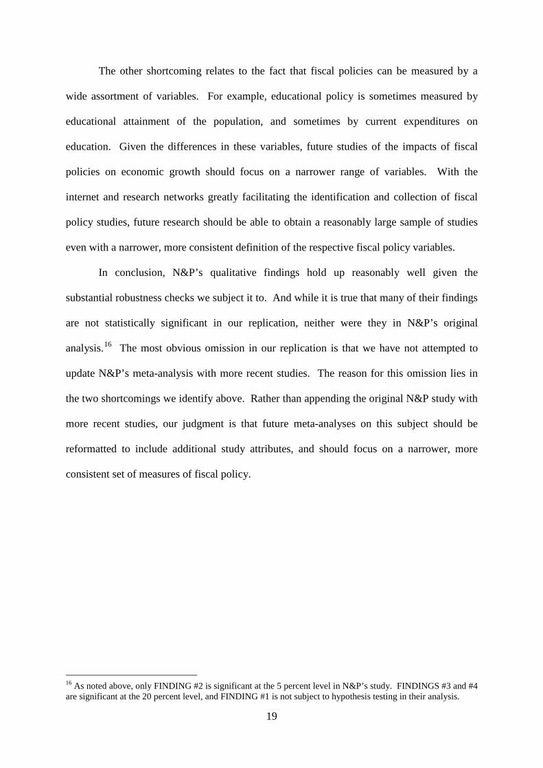
TABLE 3B investigates N&P’s other three findings. These findings all relate to

significant differences in the proportion of studies confirming the conventional prior across

the following pairs of study attributes: (i) “Conventional growth regressions” versus “Other

types of studies;” (ii) “Conventional growth regressions that include initial income” versus

“Conventional growth regressions that do not include initial income;” and (iii) studies

published in the “Top two tiers” of journal rankings versus studies published in other outlets.

It should be noted that N&P used the (generous) significance level of 0.20 in rejecting

independence across pairs of attributes. Their study calculated a p-value of 0.174 and 0.158

for the test of differences associated with conventional growth studies that did/did not include

initial income, and the test of differences for high versus lower ranked journals.

We are unable to find statistical support for any of N&P’s findings using our

reclassified sample. All of our observed differences in sample proportions are insignificant at

the 20 percent level. The closest we come to corroborating N&P is FINDING #2, where we

also find that conventional growth regressions are less likely to support the conventional prior

than other types of studies, and the associated p-value is 0.227.

Summarizing our findings to this point, we find that the classification of studies

involves a number of subjective judgments that impact the conclusions one draws from a

meta-analysis. To the best of our knowledge, the degree to which subjectivity can affect

meta-analysis outcomes has not been explicitly discussed (though it frequently mentioned in

general terms). This subjectivity may be less of a problem for disciplines where the studies

are primarily controlled experiments, with a limited number of controlling variables and

methodologies. But in economics, where the data and empirical specifications vary greatly,

and where a wide variety of econometric procedures are employed, it should be common

practice for researchers to report how they classified the individual studies in their sample.

The reason for this is that economics studies are likely to be characterized by a greater degree

10

of subjectivity. The N&P study is a good role model in this regard, as their Table 2 reports

attribute details for each of the studies in their sample.

The next section examines the robustness of these results to a variety of alternative

empirical procedures. Before doing so, and partly to motivate the procedures we employ, we

discuss additional issues associated with the application and interpretation of the meta-

analysis procedure as it applies to fiscal policies.

In assessing the growth effects of tax and spending policies, N&P included estimated

fiscal impacts that differed in their treatment of the government budget constraint. This

affects the size and significance of the fiscal policy variables, as well as their interpretation.

For example, Evans & Karras (1994) estimate a regression with US state GDP as the

dependent variable. The fiscal policy variables are public capital stock and state-level

spending on education. Helms (1985) estimates a regression with US state personal income

as the dependent variable. Right hand side explanatory variables include a fully-specified

government budget constraint with multiple categories of revenue and spending variables,

including education spending. The omitted budget category is transfer payments. The

opportunity costs of education spending in the two studies interpretation of the education

coefficients in the two studies differs greatly. In E&K, the coefficient represents the impact

of increased education spending funded by tax increases, increased intergovernmental

revenues, and/or decreases in spending in other areas.5 In contrast, the coefficient on the

education variable in the Helms study represents the impact of increased education spending

funded by decreased transfer payments. Given that the implied funding source for education

spending is different in the two studies, we should not be surprised if the sizes and signs of

the respective coefficients differ.

5 As a practical matter, borrowing for current spending is not feasible given that most states have a balanced budget requirement.

11

As noted by N&P6, a related concern has to do with the use of different measures of

the same “fiscal policy.” For example, N&P cite Barro (1991) as a study that estimates the

effect of education on economic growth. As his measure of education, Barro uses school

enrolment rates at the secondary and primary levels. In contrast, the aforementioned Evans &

Karras (1994) use total state spending on education. And Helms (1985) decomposes overall

state spending into spending on local schools and spending on higher education.

Another issue relates to the handling of multiple estimates from a single study. N&P

typically include only one observation per fiscal policy per study.7 However, a given paper

may have 10, 20, or more estimates associated with a single fiscal policy. For example, Ram

(1986) reports no less than 164 individual coefficient estimates for various measures of

public infrastructure (across different countries). There is no unique way to condense these

to a single outcome category. To explore what difference this makes, the next section

expands the analysis to include every estimate of the impact of fiscal policies in the full

sample of studies.

As is often the case, addressing one issue raises another. If multiple regressions from

the same paper are reported as separate observations, what should one do in those cases

where separate regressions are estimated for individual subsamples, accompanied by

regression results for the full sample? For example, Assane & Pourgerami (1994) report

separate regressions for the subsamples, 1970-1979 and 1980-1989; along with the full

sample, 1970-1989. Our approach is to include the regression from each sample as a separate

6 N&P note (page 110), “Growth studies use a wide range of statistical proxies to measure the level of education of the work force or actual educational expenditure by government (see Poot, 2000 for some examples). The effect of education quality (e.g., as measured by internationally comparable test scores) is likely to be more important than school attainment per se (see Barro, 2001).” 7 N&P’s reliance on the authors’ own evaluations leads to some inconsistencies in how findings across different fiscal categories are handled. For example, three observations are associated with Evans and Karras (1994), one each for the fiscal policies of education, government consumption, and infrastructure. In contrast, only one observation is associated with Helms (1985), despite the fact that he includes multiple categories of fiscal spending variables.

12

observation. The next section investigates robustness across alternative approaches for

addressing these issues.

IV. ROBUSTNESS CHECKS

Much of N&P’s analysis consists of either (i) 95% confidence intervals around the sample

proportion of studies that confirm the conventional prior, or (ii) tests of differences in sample

proportions for different pairs of study attributes. There are two shortcomings of these

approaches. Firstly, they ignore the influence of other variables that may affect the likelihood

that a given study supports the conventional prior.8 For example, education studies may tend

to support the conventional prior, on average, if a disproportionate number of these consist of

conventional growth studies. To properly test whether education studies are more likely to

support the conventional prior after controlling for other factors, we should employ an

estimation procedure that includes other explanatory variables

Secondly, when N&P construct their 95% confidence intervals, they treat the

outcomes of studies as binary, as either supporting the conventional prior or not. So, if 75%

of studies for a given fiscal policy found a “conclusively positive effect” with 25% being

inconclusive, this would be treated identically to a case with 75% conclusively positive and

25% conclusively negative.

To address the gradations of confirmation for the conventional prior, we use an

ordered logit estimation methodology that allows for each of three outcome categories. The

dependent variable CONFIRMS is ordered from lowest to highest values depending on

whether the coefficient/study rejects, is inconclusive, or supports the conventional prior.

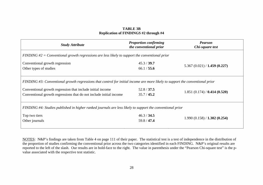
TABLE 4 reports the distribution of fiscal policy studies with respect to their support

for the conventional prior. For example, 91.7 percent of the education observations in N&P’s

original dataset confirm the conventional prior. In contrast, 75 percent of the observations in

8 To some extent, N&P address this through their use of “rough set” analysis.

13

our reclassified sample support the prior. We also include distributions for a third sample,

identified here at “Multiple Observations Per Study.” This sample expands the reclassified

sample by including every estimated coefficient reported in these studies. It is described in

greater detail below.

One complication with ordered logit/probit is that it assumes homoskedasticity.

Unlike in linear models, in nonlinear models heteroskedasticity causes coefficient estimates

to be biased and inconsistent (Williams, 2010). Furthermore, we might expect

heteroskedasticity to be an issue with N&P’s data set because the studies span different fiscal

categories. As discussed above, some of the fiscal study categories may be less/more

homogeneous than others. Defence studies are likely to use similar measures of fiscal policy

(military expenditures per capita or as a share of GDP). In contrast, public infrastructure

spending is often broken down by category (e.g., transportation spending, all public capital

expenditures, etc.). One would expect the latter to lead to greater heterogeneity in effects.

Accordingly, we first test whether our model specifications satisfy the assumption of

homoscedasticity. If our tests indicate that the model violates the assumption of “parallel

lines,” we employ a generalized ordered logit procedure that explicitly incorporates

heteroskedasticity.9

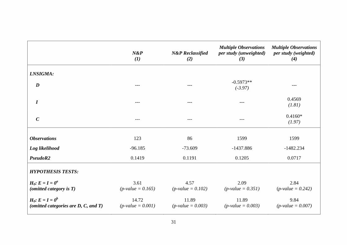
TABLE 5 reports our results in two parts. The top section of the table reports ordered

logit/generalized ordered logit estimation results for the “mean” component of the likelihood

function (cf. “CONFIRMS”). The generalized ordered logit results include coefficient

estimates for the variables in the “variance” component of the likelihood function (cf.

“LNSIGMA”). These are reported in the middle section of the table. The bottom section of

the table reports the results of our hypothesis tests (to be described below).

9 We use the oglm procedure developed for Stata and described by Williams (2010).

14

For explanatory variables, we include all the variables that allow us to test N&P’s

four findings. Fiscal policies are represented by dummy variables indicating whether the

study/coefficient is associated with education (E), public infrastructure (I), defence (D), or

government consumption (C). On the basis of TABLE 4, our empirical analysis holds out the

dummy variable for taxation studies, T, so that it serves as the reference category. We also

include dummy variables to indicate whether the study employed a conventional growth

equation (Growth), and, if so, whether the growth equation included initial income as a

control variable (Growth_Initial); along with a dummy variable to indicate that the article

was published in a highly ranked journal (Top2Journal).

Four different samples/estimation methodologies are employed. Column (1) of

TABLE 5 reports the results of an ordered logit equation using N&P’s original sample of 123

observations. Column (2) repeats the estimation, except that it uses the 86 observations from

the reclassified sample we describe in the previous section. Column (3) uses generalized

ordered logit estimation on an expanded sample of observations that includes every relevant

coefficient estimate in the reclassified sample. As noted above, some of these studies report a

large number of estimates, so that the size of this sample is 1599 observations. One potential

criticism here is that studies that report many coefficient estimates are more heavily weighted

than those that report few coefficient estimates. Given that the number of coefficients per

study ranges from a minimum of 1 to a maximum of 164, with a median value of 10, the

degree of disproportionate weighting across the 64 studies is substantial.

To address this concern, Column (4) repeats the generalized ordered logit estimation,

but weights each observation by the inverse of the number of the coefficients in each study.

Thus, an observation from a study that reports only one coefficient estimate receives 10 times

15

the weight as each of the ten observations from a study that reports 10 coefficient estimates.10

As there is no generally accepted procedure in the meta-analysis literature for how to weight

observations across studies with different numbers of estimates per study, Columns (3) and

(4) provide two “bookend” approaches to alternative weighting schemes. In addition, cluster

robust standard errors are calculated for the generalized ordered estimation of Columns (3)

and (4), with clustering by study.11

Logit/probit coefficient estimates are difficult to interpret, and this is even truer for

ordered logit/probit with multiple categorical variables. Positive (negative) coefficients are

associated with a greater (smaller) probability that the given variable will predict a higher

category of CONFIRMS. For example, the coefficient for the variable E, a dummy variable

indicating that the study/coefficient is associated with education, is estimated to be +1.8457

in the ordered logit regression of Column (1). This means that compared to fiscal studies on

taxation, education studies are more likely to support the prior. We can use this, and the

other coefficient estimates, to predict the probability that a given observation supports the

conventional prior. Following through on our education example, if all observations had

values E = 0, the associated average predicted probability would be 0.528. This compares to

an average predicted probability of 0.841 if observations took the value E = 1. In contrast,

the estimated coefficient for the variable C in Column (1) is -1.3679. The average predicted

probabilities when C = 0 and C = 1 are, respectively, 0.653 and 0.362.

We use the estimated coefficients to test each of N&P’s four main findings.

FINDING #1 states that “Education and Infrastructure studies are more likely to support the

10 We use the “pweights” weighting option in Stata. Conceptually, each study can be thought of sampling from a population of coefficient estimates. A study with one estimate can be viewed as having ten times the probability of sampling that estimate relative to an estimate from a study with ten estimates. This would be the case if the author of the study with one coefficient estimate reported that estimate because it is representative of other, similar estimates that were not reported. 11 Many meta-analyses also weight by size of sample, or coefficient standard deviation. We didn’t do this because the dependent variable is based on whether the respective coefficient was statistically significant, so that size of sample/standard deviation of coefficient was already included, in part, in the construction of the dependent variable.

16

conventional prior than other studies.” Given that there are five fiscal policy categories, there

is no single, straightforward way of directly testing this. Our first approach is test whether

there is a difference between education, infrastructure, and taxation studies. Based on the

distributions in TABLE 4 and the coefficients in TABLE 5, the taxation category is the most

likely candidate for the “middle” category with respect to supporting the prior. We also drop

D and C from the specification, and test whether the coefficients for E and I are different

from T, D, and C. The two approaches differ in how they treat the fiscal categories D and

C.12

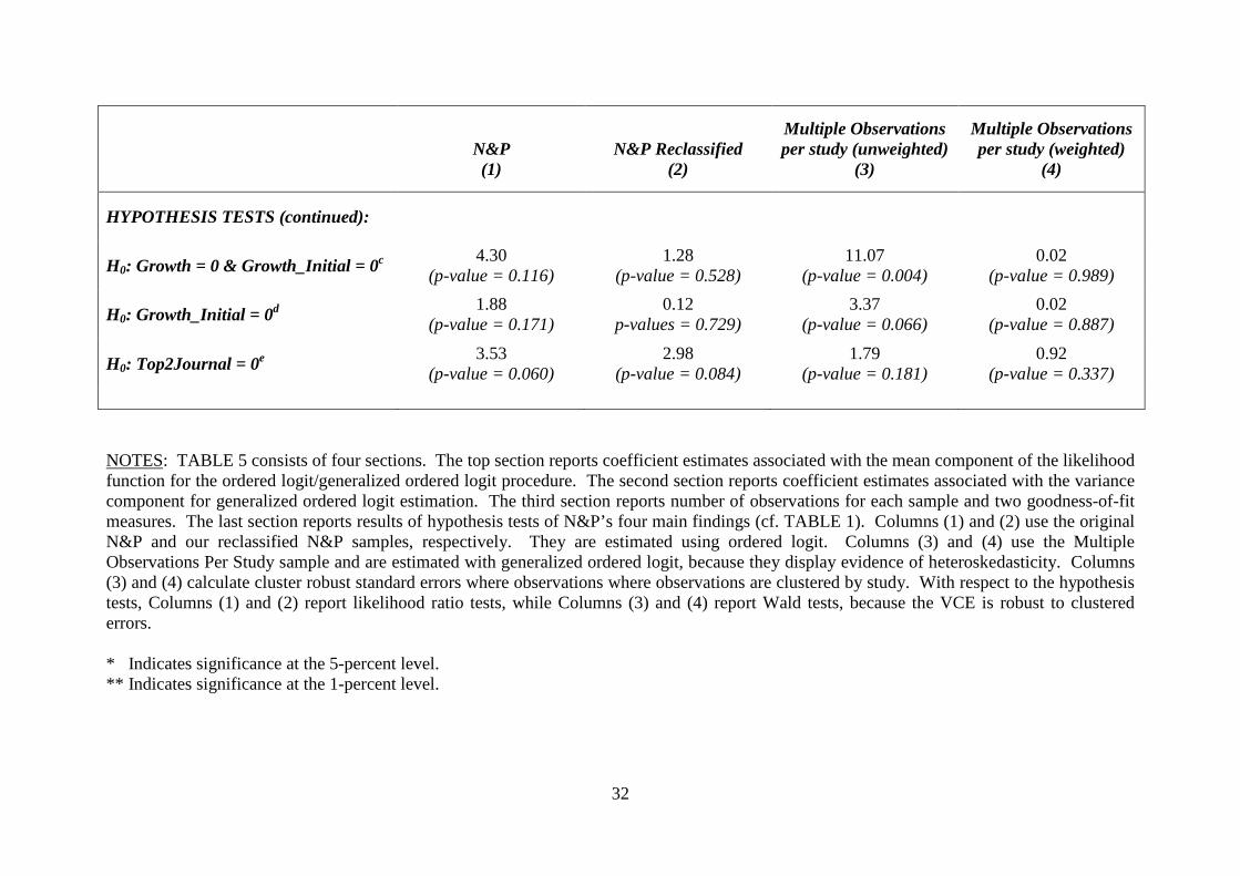
The first two rows in the bottom section of TABLE 5 (cf. “HYPOTHESIS TESTS”)

report the results of these hypothesis tests. Across all four samples/estimation procedures, we

find that education and infrastructure are not statistically distinct from taxation studies with

respect to their likelihood of confirming the conventional prior. However, if we compare

education and infrastructure studies with all other studies, lumped together as one group, we

find strong evidence that education and infrastructure are statistically distinct, which is

consistent with N&P’s FINDING #1.

The last three rows of TABLE 5 test FINDINGS #2-#4, respectively. While all four

columns produce a negative coefficient for the Growth variable, only the

Unweighted/Multiple Observations per study results of Column (3) reject the hypothesis that

conventional growth studies are no different than other studies.13 With respect to

conventional growth studies that control for initial income versus those that do not, while the

respect coefficients are all positive in TABLE 5, consistent with N&P’s finding, none are

statistically significant at the 5% (two-tailed) level of significance. Similarly, the coefficient

12 A complication arises in how to handle heteroskedasticity in the respecified models. For example, if we set I = 0 in the specification of Column (4), then I drops out of the variance component of the likelihood function. When this problem occurs, we reestimate the main specification using ordered logit, so that both the larger and the nested specifications are estimated using the same procedures. 13 When we drop the Growth_Initial variable so that the only growth variable in the equation is Growth, the estimated coefficients and p-values are, respectively: -.6464 ( 0.121), -.6466 (0.287), -.8433 (0.014)**, and -.0472 (0.951).

17

for Top2Journal is negative across all four samples/regressions, consistent with FINDING

#4, though none are statistically significant.

V. CONCLUSION

This paper replicates Nijkamp and Poot’s (2004) meta-analysis on fiscal policy and economic

growth. N&P were concerned with categorizing studies with respect to how well they

supported “conventional prior beliefs” about fiscal policies and economic growth. While that

study is now somewhat dated with respect to subsequent literature on this topic, it remains the

most recent meta-analysis study on this subject.14 We decided to replicate this study given

the importance of the subject and the fact that it continues to be actively cited in the

literature.15 Our analysis focuses on reliability and robustness, with the auxiliary goal of

developing lessons for future meta-analyses on this subject.

With respect to reliability, we find that there are a number of subjective margins

involved in categorizing research. N&P relied on the original authors’ own conclusions of

their studies. We investigated the importance of this approach by adopting a criterion that

focussed on the statistical significance of coefficient estimates. We reclassified all 93 studies

included in N&P’s sample, excluding any studies/observations that did not report relevant

standard errors/t-statistics. This eliminated review studies, other meta-analysis studies, and

studies where multiple coefficients were associated with the respective fiscal policies, among

others. It reduced the number of observations from N&P’s original sample of 123

observations, down to 86. This alternative classification procedure generally resulted in

lower rates of confirmation with respect to conventional priors (cf TABLE 4). We also

expanded the dataset by including every relevant coefficient estimate from every study for

which statistical significance could be determined. This greatly expanded the data set from

14 Though there are more recent studies that focus on a single fiscal policy area, such as public capital and military expenditures. 15 A check on Google Scholar and Scopus find numerous recent citations to N&P.

18

86 to 1599 observations, as some studies reported very large numbers of estimation results.

Finally, we investigated alternative weighting procedures, and alternative ways of calculating

standard errors (clustering on publication).

Given these substantial robustness checks, it is not surprising that we obtain mixed

results. Qualitatively, however, our results generally support N&P’s original findings:

Studies on education and public infrastructure are generally more likely to produce results

that support conventional prior beliefs. Studies published in top-ranked journals are

generally less likely to support conventional prior beliefs. And we find some evidence to

indicate that the particular specification of a growth equation (i.e., whether it included initial

income) can affect results. However, very few of our results are statistically significant.

With respect to future research in this area, we identify two shortcomings in the

original N&P study. An inspection of the original studies suggests that estimates of the

impact of fiscal policies are substantially affected by other fiscal variables in the equation.

Specifically, given that public expenditures must satisfy some kind of budget equality,

expenditure variables are implicitly measured relative to some alternative budget regime.

Greater expenditures in one fiscal area must be funded by decreased expenditures in other

areas, increased revenue enhancements, borrowing, or a combination of the above. As there

is no standard specification, studies differ in the fiscal variables they include in their

specifications. Thus, two studies examining educational expenditures can produce very

different estimates depending on the omitted fiscal variables. For example, in Helms (1985),

the omitted fiscal variable is transfer payments. Often studies do not include other fiscal

variables, so the omitted fiscal variables are a conglomeration of tax, spend, and borrow

policies. N&P make no allowance for this in their classification of study attributes. Future

research should categorize how empirical specifications address the government budget

constraint.

19

The other shortcoming relates to the fact that fiscal policies can be measured by a

wide assortment of variables. For example, educational policy is sometimes measured by

educational attainment of the population, and sometimes by current expenditures on

education. Given the differences in these variables, future studies of the impacts of fiscal

policies on economic growth should focus on a narrower range of variables. With the

internet and research networks greatly facilitating the identification and collection of fiscal

policy studies, future research should be able to obtain a reasonably large sample of studies

even with a narrower, more consistent definition of the respective fiscal policy variables.

In conclusion, N&P’s qualitative findings hold up reasonably well given the

substantial robustness checks we subject it to. And while it is true that many of their findings

are not statistically significant in our replication, neither were they in N&P’s original

analysis.16 The most obvious omission in our replication is that we have not attempted to

update N&P’s meta-analysis with more recent studies. The reason for this omission lies in

the two shortcomings we identify above. Rather than appending the original N&P study with

more recent studies, our judgment is that future meta-analyses on this subject should be

reformatted to include additional study attributes, and should focus on a narrower, more

consistent set of measures of fiscal policy.

16 As noted above, only FINDING #2 is significant at the 5 percent level in N&P’s study. FINDINGS #3 and #4 are significant at the 20 percent level, and FINDING #1 is not subject to hypothesis testing in their analysis.

20

REFERENCES Ansari, M.I., & Singh, S.K. (1997). Public spending on education and economic growth in

India: evidence from VAR modelling. Indian Journal of Applied Economics 6, 43– 64.

Aschauer, D.A. (1989c). Does public capital crowd out private capital? Journal of Monetary

Economics 24(2): 171-188. Assane, D., & Pourgerami, A. (1994). Monetary co-operation and economic growth in

Africa: comparative evidence from the CFA-zone countries. Journal of Development Studies 30, 423– 442.

Baffes, J., & Shah, A. (1998). Productivity of public spending, sectorial allocation choices

and economic growth. Economic Development and Cultural Change 46, 291–303. Bairam, E., (1988). Government expenditure and economic growth: some evidence from

New Zealand time series data. Keio Economic Studies 25, 59–66. ________ (1990. Government size and economic growth: the African experience, 1960–85.

Applied Economics 22(10): 1427-1435. Barro, R. J. (1991). Economic growth in a cross section of countries. The Quarterly Journal

of Economics 106(2): 407-443. _______ (1997).. Determinants of Economic Growth: A Cross-Country Empirical Study.

MIT Press, Cambridge, MA. Berthélemy, J.C., Herrera, R., & Sen, S. (1995). Military expenditure and economic

development: an endogenous growth perspective. Economics of Planning 28, 205– 233.

Biswas, B. & R. Ram (1986). Military Expenditures and Economic Growth in Less

Developed Countries: An Augmented Model and Further Evidence. Economic Development and Cultural Change 34(2): 361-372.

Binswanger, H.P., Khandker, S.R., & Rosenzweig, M.R. (1993). How infrastructure and

financial institutions affect agricultural output and investment in India. Journal of Development Economics 41, 337–366.

Button, K. (1998). Infrastructure investment, endogenous growth and economic convergence.

Annals of Regional Science 32, 145– 162. Cappelen, Å., et al. (1984). Military Spending and Economic Growth in the OECD Countries.

Journal of Peace Research 21(4): 361-373. Clopper, C. & E. S. Pearson (1934). The use of confidence or fiducial limits illustrated in the

case of the binomial. Biometrika 26(4): 404-413. da Silva Costa, J., Ellson, R.W., & Martin, R.C. (1987). Public capital, regional output, and

development: some empirical evidence. Journal of Regional Science 27, 419– 437.

21

Deger, S. & R. Smith (1983). Military Expenditure and Growth in Less Developed Countries.

Journal of Conflict Resolution 27(2): 335-353. Devarajan, S., et al. (1996). The composition of public expenditure and economic growth.

Journal of Monetary Economics 37(2): 313-344. Dunne, J.P. (1996). Economic effects of military expenditure in developing countries: a

survey. In: Gleditsch, N.P.,et al. (Eds.), The Peace Dividend. Elsevier Science, Amsterdam, pp. 439– 464.

Easterly, W., & Rebelo, S. (1993). Fiscal policy and economic growth: an empirical

investigation. Journal of Monetary Economics 32, 417– 458. Evans, P., & Karras, G. (1994). Are government activities productive? Evidence from a panel

of U.S. states. Review of Economics and Statistics 76, 1 –11. Faini, R., Annez, P., & Taylor, L. (1984). Defense spending, economic structure, and growth:

evidence among countries and over time. Economic Development and Cultural Change 32, 487– 498.

Garrison, C. B. & F.-Y. Lee (1995). The effect of macroeconomic variables on economic

growth rates: A cross-country study. Journal of Macroeconomics 17(2): 303-317. Gemmell, N. (1983). International comparison of the effects of non-market sector growth.

Journal of Comparative Economics 7, 368– 381. Glomm, G., & Ravikumar, B. (1997). Productive government expenditures and long-run

growth. Journal of Economic Dynamics and Control 21, 183–204. Grobar, L.M., & Porter, R.C. (1989). Benoit revisited: defence spending and economic

growth in LDCs. Journal of Conflict Resolution 33, 318– 345. Grossman, P. J. (1988). Growth in government and economic growth: The Australian

experience. Australian Economic Papers 27(50): 33-43. Guseh, J. S. (1997). Government Size and Economic Growth in Developing Countries: A

Political-Economy Framework. Journal of Macroeconomics 19(1): 175-192. Gyimah-Brempong, K. (1989). Defense spending and economic growth in subsaharan Africa:

an econometric investigation. Journal of Peace Research 26, 79–90. Hansen, P. (1994b). The government, exporters and economic growth in New Zealand. New

Zealand Economic Papers 28(2): 133-142. Hansson, P. & M. Henrekson (1994). A new framework for testing the effect of government

spending on growth and productivity. Public Choice 81(3-4): 381-401. Harmatuck, D. J. (1996). The influence of transportation infrastructure on economic

development. Logistics and Transportation Review 32(1).

22

Helms, L.J. (1985). The effects of state and local taxes on economic growth: a time series-

cross section approach. Review of Economics and Statistics 67, 574– 582. Hsieh, E., & Lai, K.S. (1994). Government spending and economic growth: the G-7

experience. Applied Economics26, 535–542. Hulten, C., & Schwab, R. (1991). Public capital formation and the growth of regional

manufacturing industries. National Tax Journal 44, 121–134. Karikari, J. A. (1995). Government and economic growth in a developing nation: the case of

Ghana. Journal of Economic Development 20(2): 85-97. Kocherlakota, N. R. & K.-M. Yi (1997). Is There Endogenous Long-Run Growth? Evidence

from the United States and the United Kingdom. Journal of Money, Credit and Banking 29(2): 235-262.

Koester, R. B. & R. C. Kormendi (1989). Taxation, aggregate activity and economic growth:

cross-country evidence on some supply-side hypotheses. Economic Inquiry 27(3): 367-386.

Kollias, C., & Makrydakis, S. (1997). Defence spending and growth in Turkey 1954 – 1993:

a causal analysis. Defence and Peace Economics 8, 189– 204. Kusi, N. K. (1994). Economic Growth and Defense Spending in Developing Countries: A

Causal Analysis. Journal of Conflict Resolution 38(1): 152-159. Landau, D. (1983). Government Expenditure and Economic Growth: A Cross-Country Study.

Southern Economic Journal 49(3): 783-792. ________ (1985). Government expenditure and economic growth in the developed countries:

1952–76. Public Choice 47(3): 459-477. ________ (1986). Government and economic growth in the less developed countries: an

empirical study for 1960-1980. Economic Development and Cultural Change 35(1): 35-75.

Lau, S.H.P., & Sin, C.Y. (1997). Public infrastructure and economic growth: time-series

properties and evidence. Economic Record 73, 125– 135. Lee, B. S. & S. Lin (1994). Government Size, Demographic Changes, and Economic Growth.

International Economic Journal 8(1): 91-108. Levine, R., & Renelt, D. (1992). A sensitivity analysis of cross-country growth regressions.

American Economic Review 82, 942–963. Lim, D. (1983). Another Look at Growth and Defense in Less Developed Countries.

Economic Development and Cultural Change 31(2): 377-384.

23

Lin, S. A. Y. (1994). Government spending and economic growth. Applied Economics 26(1): 83-94.

Lindgren, G. (1984). Review essay: armaments and economic performance in industrialized

market economies. Journal of Peace Research 21, 375– 387. Lynde, C., & Richmond, J. (1992). The role of public capital in production. Review of

Economics and Statistics 74, 37–44. _________ (1993). Public Capital and Total Factor Productivity. International Economic

Review 34(2): 401-414. MacNair, E. S., et al. (1995). Growth and Defense: Pooled Estimates for the NATO Alliance,

1951-1988. Southern Economic Journal 61(3): 846-860. Mohammed, N.A.L. (1993). Defense spending and economic growth in subsaharan Africa:

comment on Gyimah-Brempong. Journal of Peace Research 30, 95–99. Moomaw, R. L. & M. Williams (1991). Total factor productivity growth in manufacturing

further evidence from the states. Journal of Regional Science 31(1): 17-34. Morrison, C.J., & Schwartz, A.E. (1996).State infrastructure and productive performance.

American Economic Review 86, 1095–1111. Munnell, A.H. (1990). How Does Public Infrastructure Affect Regional Economic

Performance? New England Economic Review 30: 11-32. Munnell, A.H. (1992). Infrastructure investment and economic growth. Journal of Economic

Perspectives 6,189–198. Nijkamp, P. & Poot, J. (2004). Meta-analysis of the effect of fiscal policieson long-run

growth. European Journal of Political Economy 20, 91–124. Park, K. Y. (1993). `Pouring New Wine into Fresh Wineskins': Defense Spending and

Economic Growth in LDCs with Application to South Korea. Journal of Peace Research 30(1): 79-93.

Pawlak, Z. (1982). Rough sets. International Journal of Information and Computer Science

11, 341–356. Pawlak, Z. (1992). Rough Sets: Theoretical Aspects of Reasoning about Data. Kluwer,

Dordrecht. Poot, J. (2000) A Synthesis of Empirical Research on the Impact of Government on Long-

Run Growth. Growth and Change 31(4): 516-546. Ram, R. (1986). Government size and economic growth: A new framework and some

evidence from cross-section and time-series data. The American Economic Review 76(1): 191-203.

24

Rao, V.V.B. (1989). Government size and economic growth: a new framework and some evidence from crosssection and time-series data: comment. American Economic Review 79, 272–280.

Ringquist, E.J (2013). Meta-Analysis for Public Management and Policy. San Francisco,

CA: Jossey-Bass. Roux, A. (1996). Defense expenditure and economic growth in South Africa. Journal for

Studies in Economics and Econometrics 20, 19– 34. Sanchez-Robles, B. (1998). Infrastructure investment and growth: Some empirical evidence.

Contemporary Economic Policy 16(1): 98-108. Saunders, P. (1985). Public Expenditure and Economic Performance in OECD Countries.

Journal of Public Policy 5(01): 1-21. Sala-i-Martin, X. (1994). Economic growth: cross-sectional regressions and the empirics of

economic growth. European Economic Review 38, 739– 747. Sattar, Z. (1993). Government control and economic growth in Asia: Evidence from time

series data. The Pakistan Development Review: 179-197. Scully, G. (1989). The size of the state, economic growth and the efficient utilization of

national resources. Public Choice 63(2): 149-164. Singh, R. & R. Weber (1997). The composition of public expenditure and economic growth:

can anything be learned from Swiss data? Swiss Journal of Economics and Statistics. Stanley, T.D., Doucouliagos, H., Giles, M., Heckemeyer, J.H., Johnston, R.J., Laroche, P.,

Nelson, J.P., Paldam, M., Poot, J., & Pugh, G. (2013). Meta-analysis of economics research reporting guidelines. Journal of Economic Surveys 27, 390–394.

Towe, J.B., & Wright, D.J. (1995). Research published by Australian economics and

econometrics departments 1988–93. Economic Record 71, 8 – 17. van Sinderen, J. (1993). Taxation and economic growth. Economic Modelling 10, 285–300. Williams, R. (2010). Fitting heterogeneous choice models with oglm. Stata Journal 10(4):

540-567. Wylie, P.J. (1996). Infrastructure and Canadian economic growth, 1946– 1991. Canadian

Journal of Economics 29, S350– S355. Yu, W., et al. (1991). State growth rates: taxes, spending, and catching up. Public Finance

Review 19(1): 80-93. Zhang, T. & H.-f. Zou (1998). Fiscal decentralization, public spending, and economic growth

in China. Journal of Public Economics 67(2): 221-240.

25

TABLE 1 Main Findings Reported by N&P

FINDING DESCRIPTION

1 Education and Infrastructure studies are more likely to support the conventional prior than other studies.a

2 Conventional growth regressions are less likely to support the conventional prior than other studies.b

3 Conventional growth regressions that control for initial income are more likely to support the conventional prior than those that do not control for initial income.c

4 Studies published in higher ranked journals are less likely to support the conventional prior.d

a SOURCE: N&P, page 103, Table 3, (viii) Cross-tabulation of type of fiscal policy and study conclusion. b SOURCE: N&P, page 111, Table 4, Methodology. c SOURCE: N&P, page 111, Table 4, Within conventional growth regressions, (ii) By test of conditional convergence. d SOURCE: N&P, page 111, Table 4, Ranking of journal.

26

TABLE 2 Replication of Nijkamp & Poot (2004)

Study Attribute N&P (2004)

Replication (Part I)

Replication (Part II)

(i) TYPE OF FISCAL POLICY

Government size or consumption 41 41 34

Defence expenditure 21 21 10

Average or marginal tax rates 10 10 9

Public Infrastructure 39 39 25

Public expenditure on education 12 12 8 (ii) RESEARCH METHODOLOGY

Regression models with cross-sectional data 35 35 29

Regression models with panel data 46 45 35

Conventional growth regressionsa 64 64 68 Conventional growth regressions that control for

initial incomea 36 36 24

Conventional growth regressions that control for population or labour force growtha 60 60 46

Conventional growth regressions that control for the rate of investment or savingsa 52 52 55

Models using time series techniques 28 28 21

Models using other methods 14 15 1 (iii) SUPPORT FOR CONVENTIONAL PRIOR BELIEF

The conventional prior is supported 68 68 37

The study is inconclusive 44 44 39

The conventional prior is rejected 11 11 10 TOTAL OBSERVATIONS

123

123

86

NOTE: The numbers in the table represent the number of studies that correspond to the respective Study Attribute. N&P’s Table 3 report the percent of studies. The latter is easily converted to numbers using the appropriate number of observations. a N&P classify an observation as a “conventional growth regression” if (i) it is a regression model with either cross-sectional or panel data, and (ii) the dependent variable is either the growth in national income or output.

27

TABLE 3A Replication of FINDING #1

Fiscal Policy Proportion positive impact

Proportion negative impact

Proportion inconclusive impact

Conventional prior

95% C.I around proportion supporting prior

RESULT #1 = Education and Infrastructure are positively associated with economic growth.

(i) EDUCATION N&P 0.92 0.00 0.08 positive (0.57, 0.99) Replication – Part II 0.75 0.00 0.25 (0.35, 0.97) (ii) INFRASTRUCTURE N&P 0.72 0.08 0.20 positive (0.58, 0.86) Replication – Part II 0.60 0.00 0.40 (0.39, 0.79) (iii) TAXATION N&P 0.00 0.60 0.40 negative (0.26, 0.89) Replication – Part II 0.11 0.22 0.67 (-0.05, 0.49) (iv) DEFENCE N&P 0.05 0.52 0.43 negative (0.30, 0.74) Replication – Part II 0.30 0.10 0.60 (-0.09, 0.29) (v) GOVERNMENT CONSUMPTION N&P 0.17 0.29 0.54 negative (0.15, 0.43) Replication – Part II 0.18 0.38 0.44 (0.22, 0.55)

NOTES: N&P’s findings are taken from Section (viii) of Table 3 on page 103 of their paper. Our replication results are reported directly below their results in bold-face. N&P calculate 95% confidence intervals (i) for INFRASTRUCTURE, DEFENCE, and GOVERNMENT CONSUMPTION using the normal approximation, and (ii) for EDUCATION and TAXATION using the exact binomial distribution (see Footnote c of their Table 3). They do the latter because zero cells turn the ternary outcome variable into a binary variable. In contrast, we calculate exact binomial confidence intervals for EDUCATION and INFRASTRUCTURE.

28

TABLE 3B

Replication of FINDINGS #2 through #4

Study Attribute Proportion confirming the conventional prior

Pearson Chi-square test

FINDING #2 = Conventional growth regressions are less likely to support the conventional prior

Conventional growth regression 45.3 / 39.7 5.367 (0.021) / 1.459 (0.227)

Other types of studies 66.1 / 55.6

FINDING #3: Conventional growth regressions that control for initial income are more likely to support the conventional prior

Conventional growth regression that include initial income 52.8 / 37.5 1.851 (0.174) / 0.414 (0.520)

Conventional growth regressions that do not include initial income 35.7 / 45.2

FINDING #4: Studies published in higher ranked journals are less likely to support the conventional prior

Top two tiers 46.3 / 34.5 1.990 (0.158) / 1.302 (0.254)

Other journals 59.8 / 47.4

NOTES: N&P’s findings are taken from Table 4 on page 111 of their paper. The statistical test is a test of independence in the distribution of the proportion of studies confirming the conventional prior across the two categories identified in each FINDING. N&P’s original results are reported to the left of the slash. Our results are in bold-face to the right. The value in parenthesis under the “Pearson Chi-square test” is the p-value associated with the respective test statistic.

29

TABLE 4

Distribution of Fiscal Policy Variables With Respect to Support for the Conventional Prior

Variables CONFIRMS = 3 (Confirms Prior)

CONFIRMS = 2 (Inconclusive)

CONFIRMS = 1 (Rejects Prior)

SAMPLE = N&P Sample

E 91.7 8.3 0 I 71.8 20.5 7.7 T 60.0 40.0 0 D 52.4 42.9 4.8 C 29.3 53.7 17.1

SAMPLE = N&P Reclassified

E 75.0 25.0 0 I 60.0 40.0 0 T 22.2 66.7 11.1 D 10.0 60.0 30.0 C 38.2 44.1 17.6

SAMPLE = Multiple Observations Per Study

E 56.8 39.4 3.8 I 46.3 38.0 15.6 T 41.2 52.7 6.1 D 13.7 76.2 10.2 C 19.5 49.4 31.0

NOTES: The values in the table represent the distribution of fiscal policy variables across the different categories of the dependent variable, CONFIRMS, for each of the samples used in the subsequent analysis. For example, 91.7 percent of the education observations in N&P’s original dataset confirmed the conventional prior. The “N&P Sample” is the original sample of 123 observations from N&P’s study. “The “N&P Reclassified Sample” consists of 86 observations derived from our alternative approach to applying N&P’s classification scheme to the studies in their sample. The “Multiple Observations Per Study Sample” consists of an expanded sample which includes every coefficient estimate from every study for which statistical significance could be determined. All three samples are described in greater detail in the text.

30

TABLE 5 Robustness Checks: Ordered Logit and Generalized Ordered Logit Results

N&P (1)

N&P Reclassified

(2)

Multiple Observations per study (unweighted)

(3)

Multiple Observations per study (weighted)

(4)

CONFIRMS:

E 1.8457 (1.49)

2.1085* (1.98)

0.4956 (0.70)

1.1138 (1.65)

I 0.0945 (0.13)

1.2044 (1.54)

-0.1739 (-0.24)

1.2490 (1.37)

D -0.8138 (-0.98)

-1.3656 (-1.43)

-0.8408 (-1.25)

-1.4140* (-2.24)

C -1.3679 (-1.87)

0.2210 (0.29)

-1.0754 (-1.56)

-0.3016 (-0.48)

Growth -1.0629* (-2.06)

-0.6991 (-1.12)

-0.0906** (-2.82)

-0.0612 (-0.08)

Growth_Initial 0.7338 (1.37)

0.1764 (0.35)

1.0375 (1.84)

0.0763 (0.14)

Top2 Journal -0.8004 (-1.87)

-0.8420 (-1.71)

-0.5012 (-1.34)

-0.4665 (-0.96)

31

N&P (1)

N&P Reclassified

(2)

Multiple Observations per study (unweighted)

(3)

Multiple Observations per study (weighted)

(4)

LNSIGMA:

D --- --- -0.5973** (-3.97) ---

I --- --- --- 0.4569 (1.81)

C --- --- --- 0.4160* (1.97)

Observations 123 86 1599 1599

Log likelihood -96.185 -73.609 -1437.886 -1482.234

PseudoR2 0.1419 0.1191 0.1205 0.0717 HYPOTHESIS TESTS:

H0: E = I = 0a

(omitted category is T)

3.61 (p-value = 0.165)

4.57 (p-value = 0.102)

2.09 (p-value = 0.351)

2.84 (p-value = 0.242)

H0: E = I = 0b

(omitted categories are D, C, and T)

14.72 (p-value = 0.001)

11.89 (p-value = 0.003)

11.89 (p-value = 0.003)

9.84 (p-value = 0.007)

32

N&P (1)

N&P Reclassified

(2)

Multiple Observations per study (unweighted)

(3)

Multiple Observations per study (weighted)

(4)

HYPOTHESIS TESTS (continued):

H0: Growth = 0 & Growth_Initial = 0c 4.30 (p-value = 0.116)

1.28 (p-value = 0.528)

11.07 (p-value = 0.004)

0.02 (p-value = 0.989)

H0: Growth_Initial = 0d 1.88 (p-value = 0.171)

0.12 p-values = 0.729)

3.37 (p-value = 0.066)

0.02 (p-value = 0.887)

H0: Top2Journal = 0e 3.53 (p-value = 0.060)

2.98 (p-value = 0.084)

1.79 (p-value = 0.181)

0.92 (p-value = 0.337)

NOTES: TABLE 5 consists of four sections. The top section reports coefficient estimates associated with the mean component of the likelihood function for the ordered logit/generalized ordered logit procedure. The second section reports coefficient estimates associated with the variance component for generalized ordered logit estimation. The third section reports number of observations for each sample and two goodness-of-fit measures. The last section reports results of hypothesis tests of N&P’s four main findings (cf. TABLE 1). Columns (1) and (2) use the original N&P and our reclassified N&P samples, respectively. They are estimated using ordered logit. Columns (3) and (4) use the Multiple Observations Per Study sample and are estimated with generalized ordered logit, because they display evidence of heteroskedasticity. Columns (3) and (4) calculate cluster robust standard errors where observations where observations are clustered by study. With respect to the hypothesis tests, Columns (1) and (2) report likelihood ratio tests, while Columns (3) and (4) report Wald tests, because the VCE is robust to clustered errors. * Indicates significance at the 5-percent level. ** Indicates significance at the 1-percent level.

33

a This hypothesis estimates an ordered logit specification which includes fiscal policy dummies for education (E), infrastructure (I), defence (D), and government consumption (C), with the omitted fiscal category being taxation (T). Also included are the variables Growth, Growth_Initial, and Top2Journal. The hypothesis tests whether the coefficients E and I equal 0. b This hypothesis estimates an ordered logit specification which includes the fiscal policy dummies E and I, with omitted fiscal categories being D, C. and T, along with the variables Growth, Growth_Initial, and Top2Journal. The hypothesis tests whether the coefficients E and I equal 0. c This hypothesis estimates an ordered logit specification which includes the four fiscal policy dummies, along with the variables Growth, Growth_Initial, and Top2Journal. The hypothesis tests whether the coefficients for Growth and Growth_Initial equal 0. d This hypothesis estimates an ordered logit specification which includes the four fiscal policy dummies, along with the variables Growth, Growth_Initial, and Top2Journal. The hypothesis tests whether the coefficient for Growth_Initial equals 0. e This hypothesis estimates an ordered logit specification which includes the four fiscal policy dummies, along with the variables Growth, Growth_Initial, and Top2Journal. The hypothesis tests whether the coefficient for Top2Journal equals 0.

34

FIGURE 1

Number of Web of Science Articles with Meta-Analysis in The Title, By Year

35

APPENDIX I Replication of Table 3 from N&P (pages 102f.)

(i) Type of Fiscal Policy Percentage of studies

Original Replication Original Replication Original Replication Government size or consumption

33.3

33.3

Defence expenditure 17.1 17.1 Average or marginal tax rates 8.1 8.1 Public Infrastructure 31.7 31.7 Public expenditure on education 9.8 9.8

(ii) Research methodology

Regression models with cross-sectional data

28.5

28.5

Regression models with panel data 37.4 36.6 Conventional growth regressions among the above two categoriesaof which: 52.0 52.0 Control for initial income (test of conditional convergence) 56.3 56.3 Control for population or labour force growth 93.8 93.8 Control for the rate of investment or savings 81.3 81.3 Models using techniques for time series analysis 22.8 22.8 Other methods 11.4 12.2

(iii) Observations available for each study Mean Standard Deviation Min Max Original Replication Original Replication Original Replication Original Replication

Number

389.2

387.3

667

667

1

1

3304

3304

First Year 1957.6 1957.6 24.4 24.4 1831 1831 1986 1986 Time Span 28.3 28.3 25.3 25.3 1 1 161 161

36

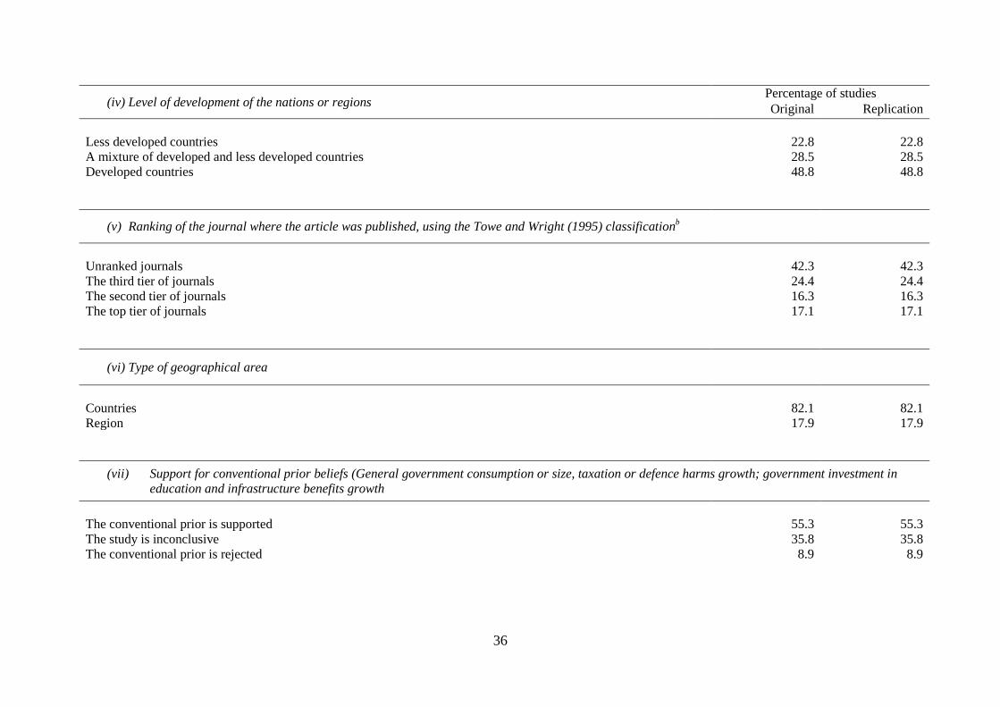
(iv) Level of development of the nations or regions Percentage of studies Original Replication

Less developed countries

22.8

22.8

A mixture of developed and less developed countries 28.5 28.5 Developed countries 48.8 48.8

(v) Ranking of the journal where the article was published, using the Towe and Wright (1995) classificationb

Unranked journals

42.3

42.3

The third tier of journals 24.4 24.4 The second tier of journals 16.3 16.3 The top tier of journals 17.1 17.1

(vi) Type of geographical area

Countries

82.1

82.1

Region 17.9 17.9

(vii) Support for conventional prior beliefs (General government consumption or size, taxation or defence harms growth; government investment in education and infrastructure benefits growth

The conventional prior is supported

55.3

55.3

The study is inconclusive 35.8 35.8 The conventional prior is rejected 8.9 8.9

37

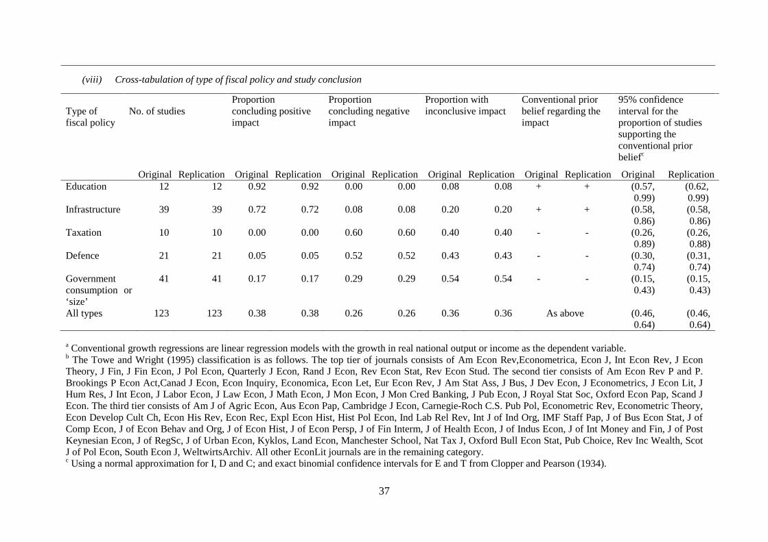
(viii) Cross-tabulation of type of fiscal policy and study conclusion

Type of fiscal policy

No. of studies

Proportion concluding positive impact

Proportion concluding negative impact

Proportion with inconclusive impact

Conventional prior belief regarding the impact

95% confidence interval for the proportion of studies supporting the conventional prior beliefc

Original Replication Original Replication Original Replication Original Replication Original Replication Original Replication Education 12 12 0.92 0.92 0.00 0.00 0.08 0.08 + + (0.57,

0.99) (0.62, 0.99)

Infrastructure 39 39 0.72 0.72 0.08 0.08 0.20 0.20 + + (0.58, 0.86)

(0.58, 0.86)

Taxation 10 10 0.00 0.00 0.60 0.60 0.40 0.40 - - (0.26, 0.89)

(0.26, 0.88)

Defence 21 21 0.05 0.05 0.52 0.52 0.43 0.43 - - (0.30, 0.74)

(0.31, 0.74)

Government consumption or ‘size’

41 41 0.17 0.17 0.29 0.29 0.54 0.54 - - (0.15, 0.43)

(0.15, 0.43)

All types 123 123 0.38 0.38 0.26 0.26 0.36 0.36 As above (0.46, 0.64)

(0.46, 0.64)

a Conventional growth regressions are linear regression models with the growth in real national output or income as the dependent variable. b The Towe and Wright (1995) classification is as follows. The top tier of journals consists of Am Econ Rev,Econometrica, Econ J, Int Econ Rev, J Econ Theory, J Fin, J Fin Econ, J Pol Econ, Quarterly J Econ, Rand J Econ, Rev Econ Stat, Rev Econ Stud. The second tier consists of Am Econ Rev P and P. Brookings P Econ Act,Canad J Econ, Econ Inquiry, Economica, Econ Let, Eur Econ Rev, J Am Stat Ass, J Bus, J Dev Econ, J Econometrics, J Econ Lit, J Hum Res, J Int Econ, J Labor Econ, J Law Econ, J Math Econ, J Mon Econ, J Mon Cred Banking, J Pub Econ, J Royal Stat Soc, Oxford Econ Pap, Scand J Econ. The third tier consists of Am J of Agric Econ, Aus Econ Pap, Cambridge J Econ, Carnegie-Roch C.S. Pub Pol, Econometric Rev, Econometric Theory, Econ Develop Cult Ch, Econ His Rev, Econ Rec, Expl Econ Hist, Hist Pol Econ, Ind Lab Rel Rev, Int J of Ind Org, IMF Staff Pap, J of Bus Econ Stat, J of Comp Econ, J of Econ Behav and Org, J of Econ Hist, J of Econ Persp, J of Fin Interm, J of Health Econ, J of Indus Econ, J of Int Money and Fin, J of Post Keynesian Econ, J of RegSc, J of Urban Econ, Kyklos, Land Econ, Manchester School, Nat Tax J, Oxford Bull Econ Stat, Pub Choice, Rev Inc Wealth, Scot J of Pol Econ, South Econ J, WeltwirtsArchiv. All other EconLit journals are in the remaining category. c Using a normal approximation for I, D and C; and exact binomial confidence intervals for E and T from Clopper and Pearson (1934).

38

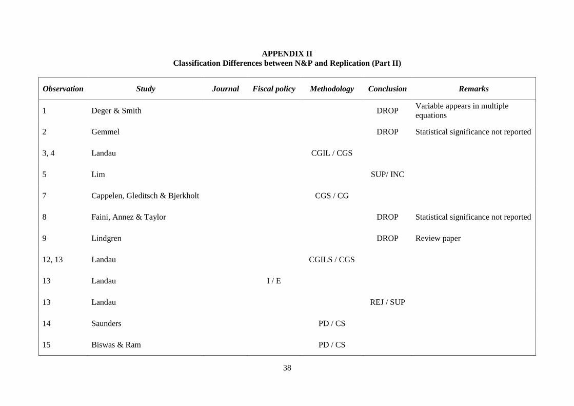
APPENDIX II Classification Differences between N&P and Replication (Part II)

Observation Study Journal Fiscal policy Methodology Conclusion Remarks

1 Deger & Smith DROP Variable appears in multiple equations

2 Gemmel DROP Statistical significance not reported

3, 4 Landau CGIL / CGS

5 Lim SUP/ INC

7 Cappelen, Gleditsch & Bjerkholt CGS / CG

8 Faini, Annez & Taylor DROP Statistical significance not reported

9 Lindgren DROP Review paper

12, 13 Landau CGILS / CGS

13 Landau I / E

13 Landau REJ / SUP

14 Saunders PD / CS

15 Biswas & Ram PD / CS

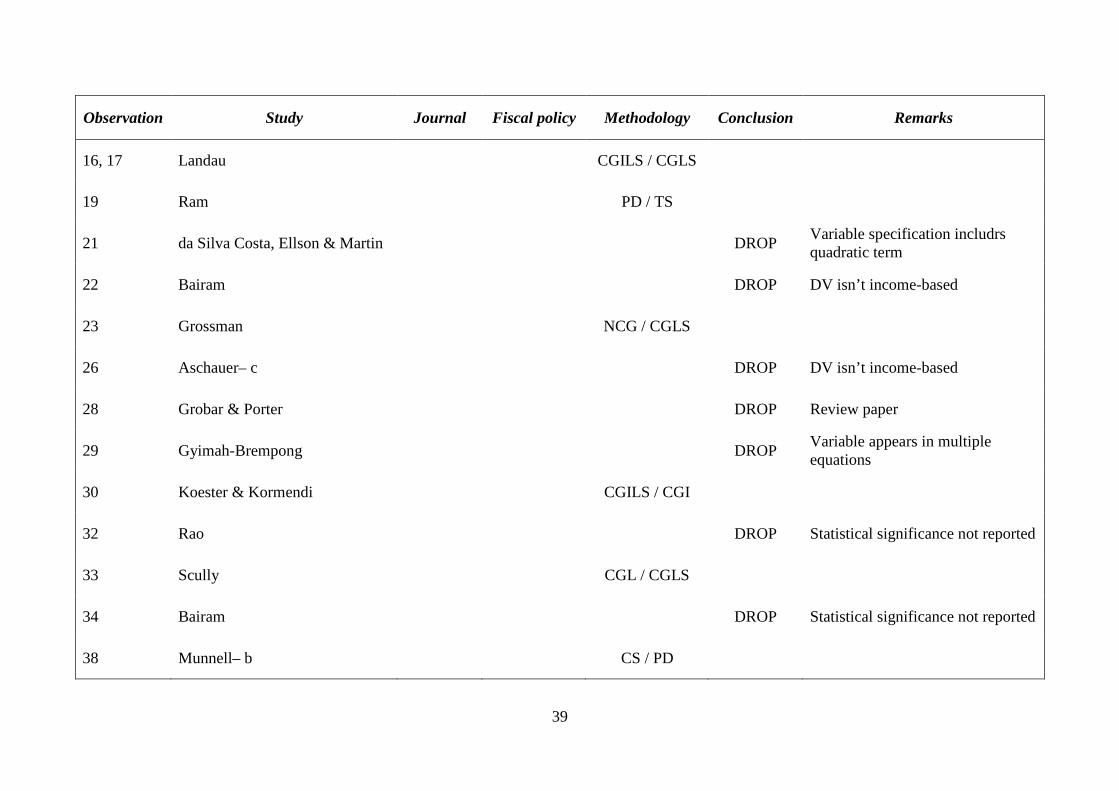
39

Observation Study Journal Fiscal policy Methodology Conclusion Remarks

16, 17 Landau CGILS / CGLS

19 Ram PD / TS

21 da Silva Costa, Ellson & Martin DROP Variable specification includrs quadratic term

22 Bairam DROP DV isn’t income-based

23 Grossman NCG / CGLS

26 Aschauer– c DROP DV isn’t income-based

28 Grobar & Porter DROP Review paper

29 Gyimah-Brempong DROP Variable appears in multiple equations

30 Koester & Kormendi CGILS / CGI

32 Rao DROP Statistical significance not reported

33 Scully CGL / CGLS

34 Bairam DROP Statistical significance not reported

38 Munnell– b CS / PD

40

Observation Study Journal Fiscal policy Methodology Conclusion Remarks

44 Hulten & Schwab NCG / CGLS

45 Hulten & Schwab DROP No result for second (other) observation

46 Moomaw & Williams SUP / INC

47 Moomaw & Williams SUP / INC

48 Yu, Wallace & Nardinelli PD / CS

48 Yu, Wallace & Nardinelli CGIL / CGI

48 Yu, Wallace & Nardinelli SUP / INC

51 Lynde & Richmond DROP DV isn’t income-based

52 Munnell DROP Review paper

54 Binswanger, Khandker & Rosenzweig DROP DV isn’t income-based

58, 59 Easterly & Rebelo DROP DV isn’t income-based over the appropriate period

60 Lynde & Richmond DROP DV isn’t income-based

61 Mohamed DROP Statistical significance not reported

41

Observation Study Journal Fiscal policy Methodology Conclusion Remarks

62 Park NCG / CG

63, 64 Sattar PD / TS

66 van Sinderen DROP Simulation study

67 Assane & Pourgerami CGILS / CGLS

72 Hansen – b NCG / CGLS

73, 74, 75 Hansson & Henrekson CS / PD

77 Hsieh & Lai DROP VAR: Insufficient statistical information

78 Kusi NCG / CG

79 Lee & Lin 1/NL

79 Lee & Lin INC / SUP

80, 81 Lin CS / PD

82, 83 Sala-i-Martin DROP Review paper

85 Berthelemy, Herrera & Sen DROP Simulation study

42

Observation Study Journal Fiscal policy Methodology Conclusion Remarks

87, 88 Garrison & Lee CGILS / CGIS

88 Garrison & Lee SUP / INC

90 Karikari NCG / CGLS

91 Macnair, Murdoch, Pi & Sandler SUP / REJ

94, 95 Devarajan, Swaroop & Zou CGL / CG

96 Dunne DROP Review paper

97 Harmatuck NCG / CGS

101 Morrison & Schwartz DROP DV isn’t income-based

102 Roux DROP Variable appears in multiple equations

103 Wylie DROP Statistical significance not reported

104 Ansari & Singh DROP VAR: Insufficient statistical information

105 Barro DROP Variable specification includes interaction term

106 Barro CGILS / CGI

43

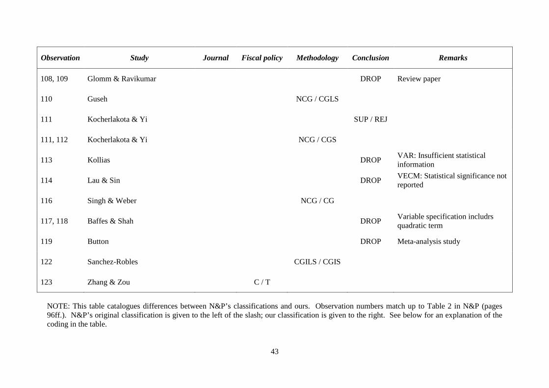
Observation Study Journal Fiscal policy Methodology Conclusion Remarks

108, 109 Glomm & Ravikumar DROP Review paper

110 Guseh NCG / CGLS

111 Kocherlakota & Yi SUP / REJ

111, 112 Kocherlakota & Yi NCG / CGS

113 Kollias DROP VAR: Insufficient statistical information

114 Lau & Sin DROP VECM: Statistical significance not reported

116 Singh & Weber NCG / CG

117, 118 Baffes & Shah DROP Variable specification includrs quadratic term

119 Button DROP Meta-analysis study

122 Sanchez-Robles CGILS / CGIS

123 Zhang & Zou C / T

NOTE: This table catalogues differences between N&P’s classifications and ours. Observation numbers match up to Table 2 in N&P (pages 96ff.). N&P’s original classification is given to the left of the slash; our classification is given to the right. See below for an explanation of the coding in the table.

44

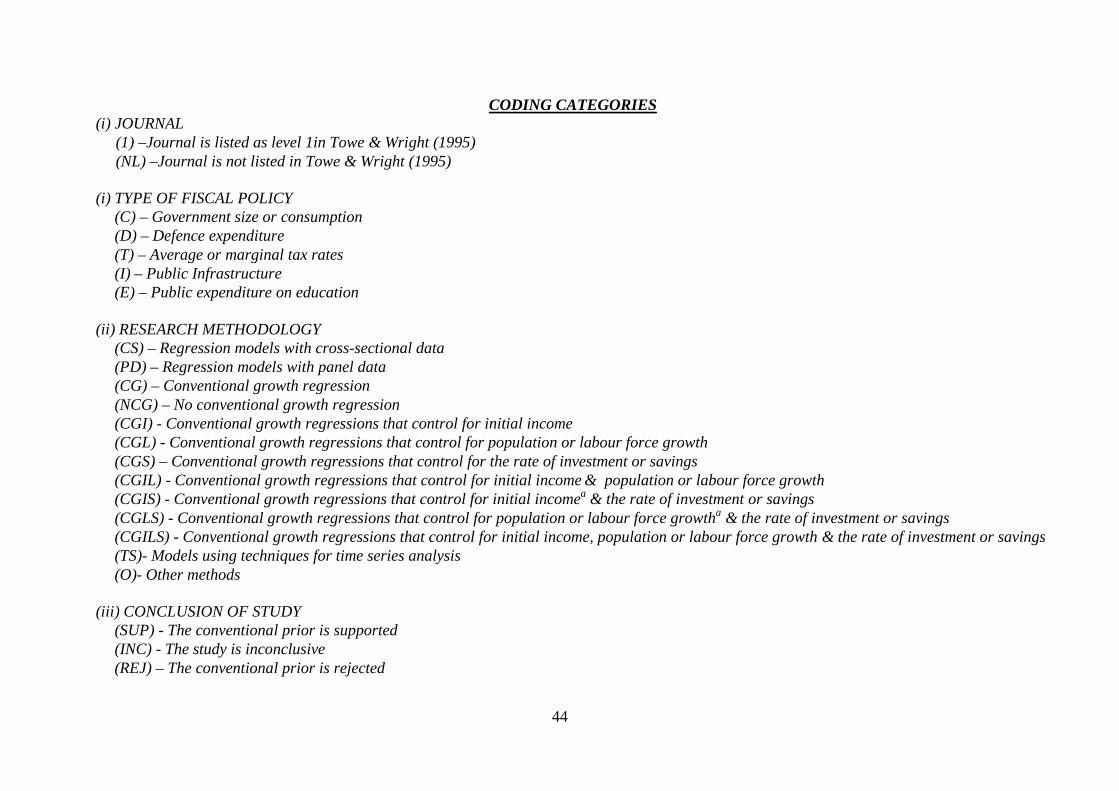
CODING CATEGORIES (i) JOURNAL (1) –Journal is listed as level 1in Towe & Wright (1995) (NL) –Journal is not listed in Towe & Wright (1995) (i) TYPE OF FISCAL POLICY

(C) – Government size or consumption (D) – Defence expenditure (T) – Average or marginal tax rates (I) – Public Infrastructure (E) – Public expenditure on education

(ii) RESEARCH METHODOLOGY

(CS) – Regression models with cross-sectional data (PD) – Regression models with panel data (CG) – Conventional growth regression

(NCG) – No conventional growth regression (CGI) - Conventional growth regressions that control for initial income

(CGL) - Conventional growth regressions that control for population or labour force growth

(CGS) – Conventional growth regressions that control for the rate of investment or savings

(CGIL) - Conventional growth regressions that control for initial income & population or labour force growth (CGIS) - Conventional growth regressions that control for initial incomea & the rate of investment or savings (CGLS) - Conventional growth regressions that control for population or labour force growtha & the rate of investment or savings (CGILS) - Conventional growth regressions that control for initial income, population or labour force growth & the rate of investment or savings (TS)- Models using techniques for time series analysis (O)- Other methods

(iii) CONCLUSION OF STUDY

(SUP) - The conventional prior is supported (INC) - The study is inconclusive (REJ) – The conventional prior is rejected