The Effect of Cryogenic Treatment on the Fatigue Life of Chrome Silicon Steel Compression Springs
169
Marquee University e-Publications@Marquee Dissertations (2009 -) Dissertations, eses, and Professional Projects e Effect of Cryogenic Treatment on the Fatigue Life of Chrome Silicon Steel Compression Springs Debra Lynn Smith Marquee University Recommended Citation Smith, Debra Lynn, "e Effect of Cryogenic Treatment on the Fatigue Life of Chrome Silicon Steel Compression Springs" (2011). Dissertations (2009 -). Paper 123. hp://epublications.marquee.edu/dissertations_mu/123
Transcript of The Effect of Cryogenic Treatment on the Fatigue Life of Chrome Silicon Steel Compression Springs
Marquette Universitye-Publications@Marquette
Dissertations (2009 -) Dissertations, Theses, and Professional Projects
The Effect of Cryogenic Treatment on the FatigueLife of Chrome Silicon Steel Compression SpringsDebra Lynn SmithMarquette University
Recommended CitationSmith, Debra Lynn, "The Effect of Cryogenic Treatment on the Fatigue Life of Chrome Silicon Steel Compression Springs" (2011).Dissertations (2009 -). Paper 123.http://epublications.marquette.edu/dissertations_mu/123

THE EFFECT OF CRYOGENIC TREATMENT ON THE FATIGUE LIFE OF CHROME SILICON STEEL COMPRESSION SPRINGS
by
Debra Lynn Smith, B.S., M.S.
A Dissertation submitted to the Faculty of the Graduate School,
Marquette University,
In Partial Fulfillment of the Requirements for
the Degree of Doctor of Philosophy
Milwaukee, Wisconsin
May 2011

ABSTRACT
THE EFFECT OF CRYOGENIC TREATMENT ON THE FATIGUE LIFE OF CHROME SILICON STEEL COMPRESSION SPRINGS
Debra Lynn Smith, B.S., M.S.
Marquette University, 2011
The purpose of this dissertation is to explore the effect of cryogenic treatment on the fatigue life of compression springs. Product manufacturers are constantly searching for ways to make their products last longer. This dissertation addresses three questions: (1) What is the effect of cryogenic treatment on the fatigue life of chrome silicon steel compression springs? Does the life increase, decrease, or remain the same? (2) What is the effect of cryogenic treatment on the Percent Load Loss (Stress Relaxation) of chrome silicon steel compression springs? (3) What are the possible changes in the material that cause these effects?
The following tests were carried out; wire tensile test, hardness test, chemical analysis, residual stress, retained austenite, lattice parameter, force vs. deflection, percent load loss (stress relaxation), fatigue, microstructures, and eta carbides.
This research produced a number of key findings: (1) The cryogenically treated springs had a longer cycle life and a higher endurance limit than the untreated springs. (2) The percent load loss (stress relaxation) of the cryogenically treated springs was similar to the untreated springs. (3) The cryogenically treated springs had a higher compressive residual stress at the surface than the untreated springs.
The conclusions of this research are that the cryogenic treatment of chrome silicon steel compression springs led to an increase in compressive residual stress on the wire surface, which in turn led to an increase in fatigue life and a higher endurance limit. A recommended future study would be to compare cryogenically treated springs to shot peened springs.

i
ACKNOWLEDGEMENTS
Debra Lynn Smith, B.S., M.S.
I owe my deepest gratitude to my dissertation committee. I am grateful to my advisor, Dr. Robert Weber, who provided me guidance and encouragement throughout this research. This dissertation would not have been possible without Mr. Luke Zubek, who brought this research topic to my attention. He was also indispensible with the fatigue testing of my springs at the Spring Manufacturers Institute. I would like to thank Dr. Raymond Fournelle for his instruction in the areas of hardness testing, tensile testing, and x-ray diffraction. I would like to thank Dr. Nicholas Nigro, who always provided sound advice and motivation. I would like to thank Dr. Robert Stango for his instruction in the many courses that I took at Marquette University.
I would like to thank the following people and organizations:
Mr. Frederick Diekman of Controlled Thermal Processing, who taught me about cryogenic treatment and processed my springs at no charge.
Mr. Larry Devine of Wisconsin Coil Spring, Inc. for manufacturing the springs at a reduced cost.
Mr. Greg Mann of Anderson Laboratories, Inc. for material analysis.
Ms. Kimberly Nickel for her instruction in the use of the Weibull++7 software.
Mr. Christopher Carpenter of Reliasoft Corporation for the free use of Weibull++7 software.
The Spring Manufacturer‟s Institute (SMI) for the free use of their software, Advanced Spring Design.
Mr. David Simonis for his information regarding Milwaukee Electric Tool Corporation‟s use of cryogenic treatment on their saw blades.
Mr. Thomas Lachtrupp and Mr. C. Chris Barger of Lambda Research, Inc. for their x-ray diffraction analyses.
Mr. Thomas Silman for his guidance in the use of the tensile test equipment.
Mr. James Pineault of Proto Manufacturing for x-ray diffraction analysis.
My parents, Max and Beatrice Smith for instilling in me a desire to learn.
Mr. William Stilley, Dr. Petar Milkovich, Mr. Nicholas Wojnar, Dr. Sung-Jin Cho, Mr. Mark Smith, Ms. Wendy Smith, and Mr. Gary Smith for their encouragement and advice.

ii
TABLE OF CONTENTS
ACKNOWLEDGEMENTS ...................................................................................... i
LIST OF TABLES ................................................................................................. iv
LIST OF FIGURES ............................................................................................... vi
NOTATION ........................................................................................................... ix
CHAPTER I INTRODUCTION ............................................................................. 1
Problem Statement ................................................................................ 1
Background and Terminology ................................................................ 1
How Springs Fail ................................................................................... 2
CHAPTER 2 REVIEW OF LITERATURE ............................................................ 6
Cryogenics............................................................................................. 6
Compression Spring Design and Testing ............................................ 11
Material Analysis ................................................................................. 12
Fatigue ................................................................................................ 18
Statistical Analysis ............................................................................... 21
CHAPTER 3 PROCEDURES AND METHODOLOGY ...................................... 24
Spring Design and Manufacturing ....................................................... 24
Spring Design .............................................................................. 24
Spring Manufacturing ................................................................... 30
Cryogenic Treatment ........................................................................... 31
Data Collection .................................................................................... 33
Mechanical Tests ......................................................................... 33
Material Characterization Tests ................................................... 35
Performance Tests ....................................................................... 43
Fatigue Tests ............................................................................... 50

Metallographic Tests .................................................................... 55
CHAPTER 4 RESULTS ..................................................................................... 58
Mechanical Tests ................................................................................. 58
Tensile Test ................................................................................. 58
Hardness Test .............................................................................. 59
Material Characterization ..................................................................... 62
Chemical Analysis ........................................................................ 62
Residual Stress ............................................................................ 65
Retained Austenite ....................................................................... 67
Performance Tests .............................................................................. 71
Force vs. Deflection ..................................................................... 71
Fatigue Tests ............................................................................... 88
Metallographic Tests ......................................................................... 110
Microstructures .......................................................................... 110
Eta Carbides .............................................................................. 114
SEM of Fractured Surface .......................................................... 115
CHAPTER 5 CONCLUSIONS AND SUGGESTIONS ..................................... 122
Conclusions ....................................................................................... 122
Suggestions for Further Study ........................................................... 122
REFERENCES ................................................................................................. 124
Appendix A Peaks used to Determine Lattice Parameters .............................. 128
Appendix B Qualitative Phase Analysis for Retained Austenite from Lambda Research ..................................................................................................... 129
Appendix C Qualitative Phase Analysis for Carbide Extraction from Lambda Research ..................................................................................................... 142

iv
LIST OF TABLES
Table 1 Heat Treat Table for Fatigue Test (Zhirafar, 2007, p. 299) ..................... 9
Table 2 Comparison of Properties of ASTM A877 and ASTM A401 Chrome Silicon Steel .................................................................................................. 13
Table 3 Inputs for Spring Calculations. .............................................................. 24
Table 4 Results of the Spring Calculations. ....................................................... 26
Table 5 Setup Parameters for Retained Austenite Measurement by Proto Manufacturing, Inc. ........................................................................................ 41
Table 6 Spacers for Percent Load Loss Test .................................................... 48
Table 7 Tensile Test Results (20 samples of each treatment group) ................. 58
Table 8 Hardness Rockwell C (converted from Vickers Hardness) ................... 61
Table 9 Chemical Analysis performed by Anderson Laboratories ..................... 63
Table 10 Gibbs Certificate of Analysis ............................................................... 64
Table 11 Residual Stress Depth Analysis. ......................................................... 67
Table 12 Volume Percent Retained Austenite using Cu Kα radiation from Lambda Technologies, Inc. ........................................................................... 69
Table 13 Volume Percent Retained Austenite using Cr Kα radiation from Proto Manufacturing, Inc. ........................................................................................ 69
Table 14 R-values for Phases from Proto Manufacturing, Inc. .......................... 70
Table 15 Lattice Parameter, a (Å). ..................................................................... 71
Table 16 Summary of Trial 1 ............................................................................. 73
Table 17 Summary of Trial 2 ............................................................................. 74
Table 18 Comparison of Loads for Trial 2 ......................................................... 75
Table 19 Percent Decrease from Trial 1 to Trial 2 ............................................. 76
Table 20 Loads of Unbroken Springs after Fatigue Testing ............................... 78
Table 21 Table Comparing Fatigue Tests 1-6. ................................................... 88

v
Table 22 Fatigue Test 1 Data. ............................................................................ 90
Table 23 Fatigue Test 2 Data ............................................................................. 91
Table 24 Fatigue Test 3 Data ............................................................................. 92
Table 25 Fatigue Test 4 Data ............................................................................. 93
Table 26 Fatigue Test 5 Data ............................................................................. 94
Table 27 Fatigue Test 6 Data ............................................................................. 95
Table 28 Fatigue Test 2 - Fatigue Test 5 Data ................................................. 102
Table 29 Estimated Endurance Limit ................................................................ 109
Table 30 Eta Carbides ...................................................................................... 115
Table 31 Peaks Used to Determine Lattice Parameters ................................... 128

vi
LIST OF FIGURES
Figure 1. Shear Stresses acting on wire and coil (Hamrock, 1999, p. 743). ......... 5
Figure 2. The fourteen Bravais lattices. (Cullity, 2001, p. 45). .............................. 7
Figure 3. Cryogenic Cycle. (Controlled Thermal, 2008) ...................................... 10
Figure 4. Minimum Tensile Strength vs. Wire Diameter Comparison of ASTM
A877 with ASTM A401. ............................................................................... 14
Figure 5. Retained Austenite as a function of carbon content in Fe-C alloys.
(Krauss, 2005, p. 64) ................................................................................... 15
Figure 6. Retained Austenite as a function of tempering temperature in 4340 and
4140 steels. (Williamson, 1979, p. 382) ...................................................... 17
Figure 7. Fatigue Strength Diagram (Society of Automotive Engineers, 1997, p.
64). .............................................................................................................. 20
Figure 8. Spring Specifications ........................................................................... 29
Figure 9. Applied Cryogenics, Inc. CP-500vi Cryogenic Chamber and
Specifications. (Diekman) ............................................................................ 32
Figure 10. Cryogenic Cooling Program CTP CP500-vi-002. .............................. 33
Figure 11. Location and orientation of Residual Stress Measurement on the
inside surface of coil at mid spring height. ................................................... 37
Figure 12. Instron Model 3345 Tester (uncompressed spring). .......................... 44
Figure 13. Instron Model 3345 Tester (compressed spring). .............................. 45
Figure 14. Assembly for Percent Load Loss Test. .............................................. 49
Figure 15. Fatigue Testing Setup of LST5000 Machine (uncompressed). .......... 52
vii
Figure 16. Fatigue Testing Setup of LST5000 Machine (compressed). .............. 53
Figure 17. Hardness Histogram. ......................................................................... 59
Figure 18. Residual Stress Distribution. ............................................................. 65
Figure 19. Percent Load Loss Test: 250°F (121°C), 1.484 in. (37.7 mm) Spring
Height. ......................................................................................................... 80
Figure 20. Percent Load Loss Test, 250°F (121°C), 1.129 in. (28.7 mm) Spring
Height. ......................................................................................................... 81
Figure 21. Percent Load Loss Test, 350°F (177°C), 1.484 in. (37.7 mm) Spring
Height. ......................................................................................................... 82
Figure 22. Percent Load Loss Test, 350°F (177°C), 1.129 in. (28.7 mm) Spring
Height. ......................................................................................................... 83
Figure 23. Percent Load Loss Test, 450°F (232°C), 1.484 in. (37.7 mm) Spring
Height. ......................................................................................................... 84
Figure 24. Percent Load Loss Test, 450°F (232°C), 1.129 in. (28.7 mm) Spring
Height. ......................................................................................................... 85
Figure 25. Percent Load Loss Test, 550°F (288°C), 1.484 in. (37.7 mm) Spring
Height. ......................................................................................................... 86
Figure 26 .Percent Load Loss Test, 550°F (288°C), 1.129 in. (28.7 mm) Spring
Height. ......................................................................................................... 87
Figure 27. Haigh Diagram of Fatigue Tests 1-6. ................................................. 89
Figure 28. Fatigue Test 2: 135.52 ksi mean stress, 57.95 ksi amplitude stress. 97
Figure 29. Fatigue Test 3: 110.69 ksi mean stress, 57.95 ksi amplitude stress. 98
Figure 30. Fatigue Test 4: 85.85 ksi, mean stress, 57.96 ksi amplitude stress. . 99

viii
Figure 31. Fatigue Test 5: 69.29 ksi mean stress, 57.95 ksi amplitude stress. 100
Figure 32. B90 Life Bar Chart ........................................................................... 103
Figure 33. Characteristic Life Bar Chart. .......................................................... 103
Figure 34. B50 Life Bar Chart. .......................................................................... 104
Figure 35. B10 Life Bar Chart. .......................................................................... 104
Figure 36. S-N Diagram, B90 Life, MLE. .......................................................... 105
Figure 37. S-N Diagram Characteristic Life B63.2. ........................................... 106
Figure 38. S-N Diagram, B50 Life, MLE. ......................................................... 107
Figure 39. S-N Diagram, B10 Life, MLE. .......................................................... 108
Figure 40. Microstructure of Group 1. ............................................................... 111
Figure 41. Microstructure of Group 2. ............................................................... 112
Figure 42. Microstructure of Group 3. ............................................................... 113
Figure 43. Microstructure of modified Group 1 wire: Austenitized at 1600°F
(871°C) for 30 minutes, water quenched, tempered at 482°F (250°C) for 1
hour. .......................................................................................................... 114
Figure 44 .Sample 3-151 Low Magnification SEM. ........................................... 117
Figure 45. Sample 3-151 High Magnification SEM Upper Right Quadrant. ...... 118
Figure 46. Sample 3-151 High Magnification SEM Lower Right Quadrant. ...... 119
Figure 47. Sample 3-151 High Magnification SEM Lower Left Quadrant. ........ 120
Figure 48. Sample 3-151 High Magnification SEM, Upper Left Quadrant. ....... 121

ix
NOTATION
A = Wire Cross Sectional Area
C = Spring Index
c.a. = Clash Allowance
cc = Coil Clearance
Dw = Wire Diameter
Dm = Mean Coil Diameter
E = Modulus of Elasticity
f = Natural Frequency
Fmin = Minimum Force
Fmax = Maximum Force
Fs = Force at Solid
F.S. = Factor of Safety at Solid
G = Shear Modulus
Goodman F.S. = Goodman Factor of Safety
ID = Inside Diameter
J = Polar Moment of Inertia
k = Spring Stiffness
Kd = Transverse Shear Factor
KW = Wahl Correction Factor
KS1 = Initial Stress Factor
KS2 = Maximum Stress Factor
Lf = Free Length

x
Lmin = Length at Fmin
Lmax = Length at Fmax
Ls = Length at Solid
Mf = Martensite Finish Temperature
Ms = Martensite Start Temperature
Na = Active Coils
Ne = End Coils
Nt = Total Coils
OD = Outside Diameter
p = Pitch
pdf = Weibull Probability Density Function
P = Load or Force
Pa = Amplitude Load
Pm = Mean Load
PO = Original Load (for Percent Load Loss calculation)
PF = Final Load (for Percent Load Loss calculation)
r = Load Line
SC = Wahl Corrected Stress
SNf = Equivalent Fully Reversed Load
Ssa = Zimmerli Endurance Strength amplitude (un-peened)
Sse = Ordinate Intercept
Ssm = Zimmerli Endurance Strength mean (un-peened)
Ssy = Torsional Yield Strength

xi
Ssys = Torsional Yield Strength at Solid
Ssu = Ultimate Shear Strength
Sult = Ultimate Tensile Strength
T = Torque
W = Weight
α = End Conditions for stability calculation
β = Shape Parameter (or slope)
γ = Location Parameter
η = Scale Parameter
λ =Pitch Angle
ν = Poisson‟s Ratio
ρ = Correlation Coefficient
σp1 = Principle Stress
σp2 = Principle Stress
τa = Amplitude Shear Stress
τm = Mean Shear Stress
τmax = Maximum Shear Stress
τo = Actual Shear Stress
τs = Shear Stress at Solid
τtorsion = Torsional Shear Stress
τtransverse = Transverse Shear Stress (also called Direct Shear Stress)
τxy = Shear Stress

1
CHAPTER I
INTRODUCTION
Problem Statement
This research addresses three questions: (1) What is the effect of
cryogenic treatment on the fatigue life of chrome silicon steel compression
springs? That is, does the life increase, decrease, or remain the same? (2) What
is the effect of cryogenic treatment on the Percent Load Loss (Stress Relaxation)
of chrome silicon steel compression springs? (3) What are the possible changes
in the material that cause these effects?
Background and Terminology
The word cryogenics is derived from the Greek words Kryos (meaning
cold), and Genes (meaning born). The Cryogenics Society of America defines
cryogenic temperatures as temperatures below 120K (-244F, -153C). There are
stories of Swiss watchmakers burying newly made parts in snow, and it is well
known that companies would “age” castings by putting them outside during the
winter. (Diekman) Computer controls can now accurately control the time and
temperature of the cryogenic chamber. Parts that have been cryogenically
treated can remain in the same chamber for a hot temper immediately after being
brought back to room temperature, thus eliminating the additional handling of
parts.

2
Mold makers use cryogenic treatment to increase the life of their tooling.
Parts commonly cryogenically treated are drills, taps, lathe tools, shaper bits,
saw blades (manufactured by Milwaukee Electric Tool), punches, dies, shear
blades, slitting knives, steel rule dies, chain saws, broaches, milling tools, router
bits, forging dies, stamping dies, blanking dies, spring forming tooling, die
springs, crankshafts, pistons, piston rings, cylinders, connecting rods, wrist pins,
valves, camshafts, gears, rocker arms, push rods, axles, brake rotors and pads,
bearings, populated circuit boards, and fire arms.
Race car teams are cryogenically treating engine components, such as
valve springs, and claiming improved wear and life. It is claimed that a valve
spring can lose up to one third of its spring constant during a long race. There
are also claims of this spring constant loss being reduced from 20-30% down to
about 7% as a result of cryogenic processing. Racers do most of their testing on
the race track or on the dynamometer. These are not controlled experiments in
the classical sense, and in most cases they do not allow the results to be
published because of the risk of losing competitive advantages. (Schiradelly,
2001) There are scientific reports and journal articles on some facets of
cryogenic treatment and its improvements. Most of the articles pertain to tool
steels and wear improvements.
How Springs Fail
The highest operating stresses in springs occur at the surfaces.
(Sebastian, 2000, p. RS-1) The fatigue failures require repeated tensile stresses.

3
If a compressive residual stress can be created at the surface, an applied tensile
stress greater than this residual stress will need to be applied in order to get
repeated tensile stresses. As each part will be able to carry considerably higher
repeated tensile load before it is actually stressed in tension. (Society of
Automotive Engineers, 1997, p. 11)
The torsional stress in a helically coiled wire is a torsional shear stress given by,
( )
( )
( )
(1.1)
in Figure 1(a) where T = Torque DW = Wire Diameter J = Polar Moment of Inertia P = Load or Force Dm = Mean Coil Diameter The maximum transverse (also called direct) shear stress
can be expressed for a solid circular cross section as
(1.2)
The maximum stress occurs at the midheight of the wire, Figure 1(b)
where A = Wire Cross Sectional Area The maximum shear stress resulting from summing the
torsional and transverse shear stresses is
(1.3a)
(
) (1.3b)
(1.3c)
where Kd = transverse shear factor =
(1.4)
C = Spring Index
(SAE, 1997, p. 7) (1-5)
Figure 1(c) shows the maximum shear stress occurs at the midheight of the wire and at the inside diameter. Curvature effects are not considered. If the transverse shear factor were small relative to the torsional shear, then Kd would be equal to 1. Any contribution from the transverse shear term would make the transverse shear factor greater than 1.
The spring index C is usually between 3 and 12. If that range is used, the range of the transverse shear factor is 1.0417 to

4
1.1667. Thus, the contribution due to transverse shear is indeed small relative to that due to torsional shear. This can be used for static loading conditions and also to check if buckling is a problem.
For a curved member the stresses can be considerably higher at the inside surface than at the outside surface. Thus, incorporating curvature can play a significant role in the spring design. A curvature correction factor attributed to A.M. Wahl results in the following:
(1.6)
where
(1.7)
The first fraction of KW accounts for the curvature effect, the second fraction accounts for the transverse shear stress. This should be used for cyclic loading.
Figure 1(d) shows the stress distribution when curvature effects and both torsional and transverse shear stresses are considered. The maximum stress occurs at the midheight of the wire and at the coil inside diameter. This location is where failure should first occur in the spring. (Hamrock, 1999, p. 742-744)

5
Figure 1. Shear Stresses acting on wire and coil (Hamrock, 1999, p. 743).
(a) Pure torsional loading;
(b) transverse loading;
(c) torsional and transverse loading with no curvature effects;
(d) torsional and transverse loading with curvature effects.

6
CHAPTER 2
REVIEW OF LITERATURE
Cryogenics
Manufacturers of products are always looking for techniques to increase
the life/durability of their parts. For products that undergo any kind of load
cycling (fatigue), this involves increasing the fatigue life or the endurance limit.
One such technique is Cryogenic Treatment. According to (Carlson, 1991, p.
203-206), the process is as follows:
Cool down slowly from ambient temperature to liquid nitrogen temperature
(2.5ºC/min or 4.5ºF/min)
Maintain -315ºF (-193°C) temperature for 24 hours.
Slowly warm-up from -315ºF (-193°C) to room temperature.
Hot temper to a specified temperature and maintain for 1 hour.
Cool down to room temperature.
Cryogenic treatment has been used in this manner to increase strength,
improve dimensional stability, improve wear resistance, and relieve residual
stresses. (Carlson, 1991, p. 205)
Research has been conducted to investigate wear resistance
improvements due to cryogenic treatment. A wear resistance ratio study for 5
high carbon steels showed a 104-560% improvement from cryogenic treatment.
(Carlson, 1991, p. 203-206) Some of the improvement is attributed to conversion
of retained austenite into martensite. Some is also attributed to the precipitation

7
of fine eta carbides, which enhances the strength and toughness of the
martensite matrix; the resulting material having a more uniform hardness.
Austenite has a face-centered-cubic crystalline structure and martensite has a
body-centered-tetragonal crystalline structure. (Wurzbach) (Meng, 1994, p. 209)
Refer to Figure 2.
Figure 2. The fourteen Bravais lattices. (Cullity, 2001, p. 45).

8
A study of 19 metals (12 tool steels, 3 stainless steels, and 4 other steels)
investigated the abrasive wear resistance using two cryogenic treatment
temperatures; 77K (-196ºC, -321ºF) and 189K (-99ºC, -146ºF). The tool steels
exhibited a significant increase in wear resistance after the 77K soak and a less
dramatic increase after the 189K soak. There was an increase in wear
resistance after the cryogenic treatment for the stainless steels, but the
difference between the two treatments was less than 10%. The plain carbon
steel and the cast iron showed no improvement after either cryogenic treatment.
(Barron, 1982, p. 411)
A test sponsored by the US Army Man Tech was conducted to „study the
effects of the carburizing process and cryogenics treatments in modifying the
microstructure of the material.” The cryogenic treatment of gears made of AISI
9310 (standard helicopter transmission gear material) resulted in 50% extra
pitting resistance, and 5% more load carrying capacity. (Wurzbach) An improved
surface finish resulted from the cryogenic treatment on H.S.S. drills from an
unpublished study by Dr. Sudarshan of Materials Modification Inc. and Dr. Levine
of Applied Cryogenics. (Wurzbach)
A study of 4340 nickel-chromium-molybdenum steel showed an
improvement in fatigue life after cryogenic treatment. Four groups of samples
were fatigue tested. Refer to Table 1.

9
Table 1
Heat Treat Table for Fatigue Test (Zhirafar, 2007, p. 299)
No. Heat Treatment
2 Austenitize at 845ºC (1553ºF), oil quench, temper at 200ºC (392ºF).
4 Austenitize at 845ºC (1553ºF), oil quench, temper at 455ºC (851ºF).
6 Austenitize at 845ºC (1553ºF), oil quench, cryo, temper at 200ºC
(392ºF).
8 Austenitize at 845ºC (1553ºF), oil quench, cryo, temper at 455ºC
(852ºF).
Both cryogenically treated groups (6, 8) exhibited higher fatigue stress levels
compared to their non-treated counterparts (2, 4). The improvement was on the
order of 25-30 MPa at lifetimes of approximately 107 cycles; approximately a
7.8% increase at 455ºC (851ºF), and a 3.2% increase at 200ºC (392ºF).
(Zhirafar, 2007, p. 302)
A typical cryogenic cycle is shown below in Figure 3. It includes a temper
within the same chamber to reduce handling of parts.

10
Figure 3. Cryogenic Cycle. (Controlled Thermal, 2008)
There are several theories concerning reasons for the effects of cryogenic
treatments. (1) One theory involves the more nearly complete transformation of
retained austenite into martensite. This theory has been verified by x-ray
diffraction measurements. (2) Another theory is based on the strengthening of
the material brought about by precipitation of submicroscopic carbides as a result
of the cryogenic treatment. (3) Allied with this is the reduction in internal stresses
in the martensite that happens when the submicroscopic carbide precipitation
occurs. A reduction in microcracking tendencies resulting from reduced internal
stresses is also suggested as a reason for improved properties. (Carlson, 1991,
-418
-318
-218
-118
-18
82
182
282
382
-250
-200
-150
-100
-50
0
50
100
150
200
0 10 20 30 40 50 60
Te
mp
era
ture
(°F
)
Te
mp
era
ture
( °
C)
Hours
Cryogenic Cycle (Controlled Thermal Processing, Inc.)
-187 ºC (-305 ºF) for 20 hours
Temper Temperature 149 ºC (300 ºF) for 2-3 hours
-26 ºC / hr (-47 ºF / hr)
+64 ºC / hr (115 ºF / hr) for 2 hours
+14 ºC / hr (+25 ºF / hr) for 15 hours
Allow to Cool to Room Temperature

11
p. 203-206) This includes relief of tensile residual stresses. It may also include
addition of compressive residual stresses. (4) The atomic spacing within freshly
formed martensite decreases upon cooling and remains less than original
martensite atomic spacing even upon heating. (Electric Power Research Institute
(EPRI), 1999)
Compression Spring Design and Testing
Many accepted formulas exist for spring design. A stress calculation
needs to be modified with a stress correction factor.
The Wahl corrected shear stress formula is:
(Society of Automotive Engineers, 1997, p. 61) (2-1)
where KW = Wahl Correction Factor
KW increases with greater curvature of the coiled wire. Greater curvature
is equivalent to a smaller spring index, C, which is defined as the ratio of the
mean coil diameter to the wire diameter.
(Society of Automotive Engineers, 1997, p. 7) (2-2)
(Wahl, 1944/1996, p. 56) (2-3)
Larger diameters are easier to measure volume percent retained austenite
and residual stresses. Too high of a Spring Index, C makes it difficult to maintain
a consistent pitch/coil spacing. This inconsistency in pitch creates varying free
lengths, varying diameters and therefore varying rates and loads. (DeFord, 2006,
p. 25-26)

12
An integer number of coils will give significantly lower non-axial forces
than fractional number of coils. (Hayes, 2006, p. 63-64) The stresses induced
from coiling can produce stress cracks in the material if not stress relieved.
(DeFord, 2006, p. 47-48) Mr. Luke Zubek recommended 750°F (399°C) as a
stress relief temperature for Chrome Silicon steel springs. Wire of Chromium
Silicon steel temper softens only above about 425°C (800°F). (Godfrey, 1990, p.
311)
The most popular commercially acceptable technique to improve the
fatigue life of compression springs is shot peening. Shot peening has increased
the fatigue limit for springs by: 54% for Carbon Spring Steel SAE 1074, 60% for
Alloy Spring Steel SAE 6150, 100% for Stainless Steel Type 302, and 100% for
Phosphor Bronze SAE 81. (Society of Automotive Engineers, 2001, p. 5) Shot
peening can be successfully carried out on wire sizes in excess of 0.75 mm (0.03
in). (Society of Automotive Engineers, 1997, p. 11)
To avoid resonance, the natural frequency should be at least 13 times the
operating frequency. (Sebastian, 2000, p. S-16)
Material Analysis
Springs for this research were made from ASTM A877/A877M Valve
Spring Quality Chrome Silicon steel wire. A comparison of the properties to
those of ASTM A401/A401M AISI 9254 Chrome Silicon steel wire is shown in
Table 2 below.

13
Table 2
Comparison of Properties of ASTM A877 and ASTM A401 Chrome Silicon Steel
ASTM A877/A877M Valve Spring Quality Chrome Silicon Wire
ASTM A401/A401M Chrome Silicon Wire
(AISI 9254) Ref
Carbon 0.51 – 0.59 % 0.51 – 0.59 % (ASTM International, 2005)
(ASTM International, 2003)
Manganese 0.50 – 0.80 % 0.60 – 0.80 % (ASTM International, 2005)
(ASTM International, 2003)
Phosphorous 0.025 % Max 0.035 % Max (ASTM International, 2005)
(ASTM International, 2003)
Sulfur 0.025 % Max 0.040 % Max (ASTM International, 2005)
(ASTM International, 2003)
Silicon 1.20 – 1.60 % 1.20 – 1.60 % (ASTM International, 2005)
(ASTM International, 2003)
Chromium 0.60 – 0.80 % 0.60 – 0.80 % (ASTM International, 2005)
(ASTM International, 2003)
Density 7850 kg/m3
0.284 lb/in3
7850 kg/m3
0.284 lb/in3
(Society of Automotive Engineers, 1997, p. 23)
(Beuter, 2002, p. 16)
Minimum Tensile Strength 1690 – 2100 MPa
245 – 305 ksi
1620 – 2069 MPa
235 – 300 ksi
(Beuter, 2002)
Modulus of Elasticity (E) 207,000 MPa
30 * 106 psi
207,000 MPa
30 * 106 psi
(Beuter, 2002)
Design Stress % Minimum Tensile
45 45 (Beuter, 2002)
Modulus in Torsion (G) 79,300 MPa
11.5 * 106 psi
79,300 MPa
11.5 * 106 psi
(Beuter, 2002)
Available Wire sizes 0.5 – 9.5 mm
0.020 – 0.375 in.
0.8 – 18.0 mm
0.032 – 0.687 in.
(ASTM International, 2005)
(ASTM International, 2003)
Maximum Operating Temperature
245°C
475°F
245°C
475°F
(Beuter, 2002)
Rockwell Hardness C48-55 C48-55 (Beuter, 2002)

14
In addition to improved surface quality, the Valve Spring Quality wire has
slightly higher tensile strength. This is shown in Figure 4 below.
Figure 4. Minimum Tensile Strength vs. Wire Diameter Comparison of ASTM A877 with ASTM A401.
Low retained austenite content and fine austenitic grain sizes create a
microstructure of finely dispersed retained austenite and tempered martensite.
This prevents the nucleation of fatigue cracks or retards fatigue crack initiation
until very high stresses are achieved. (Herring, 2005, p. 14)
The martensite finish temperature, Mf, or the temperature at which the
martensite transformation is complete in a given alloy, is a function of carbon
y = 230,843.4066x-0.0808 R² = 0.9342
y = 216,873.0056x-0.1033 R² = 0.9858
200,000
220,000
240,000
260,000
280,000
300,000
320,000
0.000 0.100 0.200 0.300 0.400 0.500 0.600 0.700
Min
imu
m T
en
sil
e S
tren
gth
, p
si.
Wire Diameter, inches
Minimum Tensile Strength vs. Wire Diameter
ASTM A877
ASTM A401
Power (ASTM A877)
Power (ASTM A401)

15
content. Refer to Figure 5. The Mf drops below room temperature in alloys
containing more than about 0.3% Carbon. (Krauss, 2005, p. 63)
Figure 5. Retained Austenite as a function of carbon content in Fe-C alloys. (Krauss, 2005, p. 64)
Alloying elements that stabilize austenite increase the amount of retained
austenite at any given carbon level and temperature. Alloying elements also
influence the martensite start temperature, Ms. Chromium lowers the Ms up to
5%. (Krauss, 2005, p. 63-64)

16
Too much retained austenite can result in lower elastic limits, reduced
hardness, lower high cycle fatigue life, and dimensional instability. Too little
retained austenite, can result in poor fracture toughness and reduced low cycle
fatigue and rolling contact fatigue life. (Krauss, 1995)
In addition to increasing hardenability, certain alloying elements also help
to retard the rate of softening during tempering. The most effective elements are
strong carbide formers such as chromium, molybdenum, and vanadium. Low
carbon steels without these elements soften rapidly with increasing tempering
temperature. (Krauss, 2005, p. 333)
Retained austenite level of 2% was found in as quenched AISI 4340
(nickel-chromium-molybdenum steel) and 4% in as quenched AISI 4130
(chromium-molybdenum steel), which are similar to the spring material used in
this research. Refer to Figure 6.

17
Figure 6. Retained Austenite as a function of tempering temperature in 4340 and 4140 steels. (Williamson, 1979, p. 382)
Testing for very small amounts of retained austenite has been performed
using Transmission Electron Microscopy (Thomas, 1978) and Mössbauer
Spectroscopy (Williamson, 1979).

18
The supersaturation of carbon atoms provides the driving force for carbide
formation. During tempering, a transition carbide of Fe2C was designated as eta
(η) carbide. (Krauss, 2005, p. 338-339)
Characteristics of steel, such as hardenability and microstructures of
austenite transformation products, depend on austenite grain size. In the
absence of austenite itself, the austenite grain size of a steel is referred to as the
prior-austenite grain size. Etching techniques can be used to show prior-
austenite grain boundaries in hardened steels. (Krauss, 2005, p. 120-121) Fine
grain sizes increase ductile fracture stresses, and lower ductile to brittle transition
temperatures. Grain size refinement is the only mechanism that increases both
strength and toughness. (Krauss, 2005, p. 212)
Fatigue
The most familiar type of distribution function is the normal or Gaussian
distribution. Unfortunately, fatigue failures do not usually follow this type of
distribution. A Weibull distribution is commonly used. It has two parameters;
Beta is a shape parameter, and Eta is the characteristic life. A normal
distribution is a special case of the Weibull distribution with a shape factor, Beta
is approximately equal to 3.57. When evaluating fatigue data, the Weibull plot
represents the unreliability (U) of a population expressed as a function of life (x),
U = f(x). Life can be expressed in terms of time, cycles, etc. The unreliability at
any specified life is the fraction of the population expected to fail before that life is
achieved. Reliability (R) is the fraction of the population expected to survive at

19
the specified life. The sum of the Reliability and Unreliability equals one. By
definition, the best-fit line through the data on the Weibull plot represents a
confidence level of 50%. Common practice has become to state the predicted
life at 10% unreliability. This is commonly referred to as the B10 life. The SAE
Standard is to state the B10 life at 50% confidence. (Stone, 2002)
One of the key limitations to the Stress-Number of Cycles curve (S-N
curve) was the inability to predict life at stress ratios different from those under
which the curve was developed. In predicting the life of a component, a more
useful presentation of fatigue life test data is the modified Goodman Diagram.
These diagrams, while still limited by specimen geometry, surface condition, and
material characteristics, enable the user to predict life at any stress ratio. The
most common format used in the spring industry has the normalized minimum
operating stress plotted along the x-axis while the normalized maximum
operating stress is plotted along the y-axis. This is shown in Figure 7. Within a
select set of spring materials, normalizing the plotted data by dividing the
material‟s tensile strength allows the use of the same diagram for a variety of
materials across their range of tensile strengths. (Stone, 2002)

20
Figure 7. Fatigue Strength Diagram (Society of Automotive Engineers, 1997, p. 64).
It is important to note that the diagram does not apply to Chrome-Silicon
and Chrome-Silicon-Vanadium alloys. Common practice based on limited
historical data, is to consider the cold wound diagrams applicable to these
materials as well. (Stone, 2002)

21
The fully reversed, bending unnotched fatigue limit of 4140 chromium-
molybdenum steel is 61,000-66,000 psi, and of 4340 nickel-chromium-
molybdenum steel is 68,000-97,000 psi. (Stephens, 2001, p. 448)
The role of compressive residual stresses in springs is known to improve
fatigue life. The common technique to create these compressive residual
stresses is shot peening. Improvement from 80,700 cycles to no failures at
1,000,000 cycles was achieved by shot peening ASTM A-401 Chrome Silicon
steel springs to a surface residual stress of 70,000 psi compression. (Hornbach,
1999)
Percent Load Loss can also be referred to as stress relaxation or creep.
Creep can cause significant permanent deformation and/or fracture and is usually intercrystalline. Creep failures have occurred in gas turbine blades due to centrifugal forces. These have been significantly overcome by using single-crystal turbine blades. (Stephens, 2001, p. 2-3)
Statistical Analysis
While the normal distribution has a number of attractive attributes and has
been the subject of many publications, it must be recognized that in spring
fatigue testing the results are usually not normal in that they cannot be plotted in
the symmetrical bell-shaped distribution curve, but instead, in a skewed curve. In
the automotive industry the Weibull plot is used because it permits straight-line
plotting of the cumulative failure probability versus life cycles on Weibull

22
probability graph paper, even when the distribution is skewed. (Society of
Automotive Engineers, 1997, p. 71)
The Weibull distribution is one of the most widely used lifetime
distributions in reliability engineering. The three-parameter Weibull Probability
Density Function (pdf) is given by:
( )
(
)
(
)
(“Weibull++7”, p. 109) (2-4)
where f(T) ≥ 0, T ≥ 0 or γ, β > 0, η > 0, -∞ < γ < ∞,
T = time to failure,
η = scale parameter,
β = shape parameter (or slope),
location parameter.
The Weibull shape parameter, β, is also known as the slope. This is
because the value of β is equal to the slope of the regressed line in a probability
plot.
The scale parameter, η, defines where the bulk of the distribution lies, or
how stretched out the distribution is. ("Weibull++7", p. 28)
The location parameter, γ, locates the distribution along the abscissa.
Changing the value of γ has the effect of “sliding” the distribution and its
associated function to the right (if γ > 0) or to the left (if γ < 0). ("Weibull++7", p.
120)
The two-parameter Weibull pdf is obtained by setting γ=0 and is given by:
( )
(
)
(
)
(“Weibull++7”, p. 110) (2-5)
Several settings were made for the analysis in this research:

23
Two Parameter Analysis
MLE (Maximum Likelihood) / SRM (Standard Regression Method)
Fischer Matrix Confidence Bound
Median Ranks ranking
In many cases when life data are analyzed, all of the units in the sample
may not have failed or the exact times-to-failure of all the units is not known.
This type of data is commonly called censored data. The most common case of
censoring is what is referred to as right censored data, or suspended data. In the
case of life data, these sets are composed of units that did not fail. ("Weibull++7",
p. 59)
MLE (Maximum Likelihood) was used instead of Rank Regression on X,
because of its advantage when data has many suspended points.

24
CHAPTER 3
PROCEDURES AND METHODOLOGY
Spring Design and Manufacturing
Spring Design
The first step was to design the springs to be tested. Spring design was
performed using commonly accepted spring formulas. Refer to Table 3 for the
geometric parameters and material properties which were used.
Table 3
Inputs for Spring Calculations.
Symbol Description English SI
Dw Wire Diameter
0.1205 in. 3.06 mm
Dm Mean Diameter
0.964 in. 24.49 mm
k Spring Stiffness 112.8 lbs/in
19.8 N/mm
Lf Free Length 1.75 in 44.5 mm
Fmin Minimum Force
30 lbs 133 N
Fmax Maximum Force
70 lbs 311 N
Sult Ultimate Tensile Strength
280,000 psi 1931 MPa
E Modulus of Elasticity 30 X 106 psi
207 X 103 MPa
G Shear Modulus
11.5 X 10⁶ psi 79 X103 MPa
Ne End Coils
2 2
Squared and Ground Ends
α End Conditions for Stability calculation 0.5 0.5
Severe Service
Ssa Zimmerli Endurance Strength amplitude (un-peened) 45,000 psi 310 MPa
Ssm Zimmerli Endurance Strength mean (un-peened)
55,000 psi 379 MPa

25
The material selected was valve spring quality chrome silicon steel wire
per ASTM A877/A877M, with a wire diameter of 0.1205 inches. Larger
diameters should be easier to measure retained austenite and residual stresses.
3 mm (0.118 in) would be preferred but 1 mm (0.039 in) should be sufficient to
measure retained austenite and residual stresses. (J. Pineault, personal
communication, February 28, 2008)
An integer number of coils gives significantly lower non-axial forces than
designs with x + ½ coils. (Hayes, 2006) The number of active coils should be
between 3 and 15. (Shigley, Mischke, & Budynas, 1963/2004)
The spring index C (ratio of mean diameter to wire diameter) should be
between 5 and 8. Too low of an index can mark the inside surface of the spring,
resulting in early breakage. The Wahl Correction Factor, KW, is inversely
proportional to the Spring Index, C. Too high of a Spring Index makes it difficult
to maintain a consistent pitch/coil spacing. This inconsistency in pitch creates
varying free lengths, varying diameters, and therefore varying rates and loads.
(Society of Automotive Engineers, 1997, p. 34) (DeFord, 2006) (L. Zubek,
personal communication, April 17, 2008) Squared and ground ends were
selected.
The stress relief selected was one hour at 700°F (371°C). Because of
chrome silicon‟s high hardness, springs need to be stress relieved within four
hours of coiling. The stresses induced from coiling can produce stress cracks in
the material if not stress relieved. (DeFord, 2006, p. 48)

26
Refer to Table 4 for the results of the spring calculations.
Table 4
Results of the Spring Calculations.
Symbol Description Equation Eq No.
Result (English)
Result (SI) Reference
Lmin Length at Minimum
Force
3-1 1.484 in. 37.7 mm N/A
Lmax Length at Maximum
Force
3-2 1.129 in. 28.7 mm N/A
C Spring Index
3-3 8 8 (Beuter, 2002,
p. 49)
KW Wahl Correction
Factor
3-4 1.18 1.18 (Wahl, 1944/
1996, p. 56)
τo Actual Shear Stress
3-5 116,282 psi 801 MPa (Wahl, 1944/1996, p. 56)
Na Active Coils
3-6 3.00 3.00 (Sebastian, 2000, p. S-26)
Nt Total coils 3-7 5 5 N/A
p Pitch
3-8 0.50 in. 12.7 mm (Beuter, 2002, p. 51)
λ Pitch Angle ( ) 3-9 9.43° 9.43° N/A
LS Solid Length
3-10 0.602 in. 15.3 mm (Beuter, 2002,
p. 51)

27
FS Force at Solid Length
( ) 3-11 129 lbs 574 N N/A
τS Shear Stress at Solid Length
3-12 215,035 psi 1,483 MPa
(Wahl, 1944/1996, p. 56)
OD Outside Diameter
3-13 1.0845 in. 27.56 mm (Mott, 1999, p. 661)
ID Inside Diameter
3-14 0.8435 in. 21.42 mm (Mott, 1999, p. 661)
c.a. Clash Allowance
3-15 0.85 0.85 (Deutschman,
1975, p. 723)
cc Coil Clearance,
in.
3-16 0.18 in. 4.6 mm (Mott, 1999, p.
674)
Stability Criteria
√ ( )
3-17 5.061 Stable
5.061 Stable
(Shigley, Mischke, &
Budynas, 1963/2004, p. 514)
Ssys Torsional Yield
Strength at Solid
3-18 154,000 psi 1,062 MPa
(Shigley, Mischke, &
Budynas, 1963/2004, p. 517)
F.S. Factor of Safety at
Solid Length
3-19 0.72 0.72 N/A
W Weight π2Dw
2DmNaγ / 4
3-20 0.029 lbs. 0.13 N (Shigley, Mischke, &
Budynas, 1963/2004, p. 520)
f Natural Frequency,
Hz
0.5sqrt(kg/W) 3-21 608.3 608.3 (Baumeister, 1916/1978, p. 5-
67)
Pm Mean Load ( )
3-22 50 lbs 222 N (Hamrock, 1999, p. 752)
Pa Alternating Load
3-23 20 lbs 89 N (Hamrock,
1999, p. 752)
τm Mean Shear Stress
3-24 83,059 psi 573 MPa (Hamrock, 1999, p. 752)

28
This analysis led to the inputs listed in the Spring Specification Sheet in
Figure 8.
τa Amplitude Shear Stress
3-25 33,223 psi 229 MPa (Hamrock, 1999, p. 752)
Ssu Ultimate Shear
Strength
3-26 186,760 psi 1288 MPa (Norton, 1998/2011, p. 793)
Ssy Torsional Yield
Strength
3-27 140,000 psi 695 MPa (Hamrock, 1999, p. 265)
Sse Fully Reversed Endurance Strength (Ordinate
Intercept of Goodman Line on Haigh
Diagram)
* (
)+
3-28 56,000 psi 386 MPa (Stephens, 2001, p. 85)
r Load Line
3-29 0.40 0.40 (Shigley, Mischke, &
Budynas, 1963/2004, p. 348)
Ssa Fully Reversed Endurance Amplitude
3-30 32,007 psi 221 MPa (Shigley,
Mischke, & Budynas, 1963/2004, p. 350)
Goodman F.S.
Goodman Factor of
Safety
*
+
3-31 0.963 0.963 (Shigley, Mischke, &
Budynas, 1963/2004, p. 350)

29
Figure 8. Spring Specifications
9
in max
1.75 in ± 0.06
1.0845 in ± 0.0180
0.8435 in ± REF
4. Load 30.00 lbs ± REF lbs @ 1.484
Load 70.00 lbs ± 5.30 lbs @ 1.129
Rate 112.80 lbs/in ± REF
0 in and 0.602
0.602
0.1205
0.964
3.00
5.00
None
6
1.484 in to 1.129
Research: The Effect of Cryogenic Treatment on the Fatigue
Life of Compression Springs.
Stress Relieve at 700ºF for 1 hour.
3. No of active coils
4. Total no. of coils ± 0.05 coils
6. Direction of helix (L, R, or optional)
2. Mean coil diameter in REF
5. Maximum solid height
7. Type of ends
in REF
1. Wire diameter in
Advisory Data
in
3. INSIDE DIAMETER
a.
b.
in. max or
in
in
lbs/in
in
a.
b.
in min. or
in
to complete specification sheetUse Run No.
COMPRESSION SPRING SPECIFICATION SHEET
between lengths of
A877
Squared and Ground
in. max or
Mandatory Specifications
a.
b.
1. FREE LENGTH
2. OUTSIDE DIAMETER
in
Special Information
1. Type of Material
2. Finish
Oil Tempered Valve
Spring Quality Chrome
Silicon per ASTM A
877/A 877M-05.
3. Squareness
4. Frequency of compression cycles/sec
7. Other
and working range in of length
5. Operating temp
6. End use of application
oF
Reset

30
Spring Manufacturing
To evaluate the effects of cryogenic treatment three groups of spring
specimens were prepared. The Group 1 springs were stress relieved at 700°F
(371°C) for one hour for stress relief after coiling. The Group 3 springs were
stress relieved at 700°F (371°C) for one hour, cryogenically treated, and then
tempered at 300°F (149°C) for 2 hours. To isolate improvements from the
cryogenic treatment from the 300°F (149°C) temper, Group 2 springs were stress
relieved at 700°F (371°C) for one hour, and then tempered at 300°F (149°C) for
2 hours.
The Wisconsin Coil Spring Corporation supplied 2,150 springs and 100
feet of wire for this research. They obtained the wire from Gibbs Wire Inc. The
wire starts out at a larger diameter. The surface is cleaned and then goes
through several draw reductions until the 0.1205 inch diameter is reached. The
wire is hardened in an oil tempering furnace. The wire passes through an
austenitizing furnace at 1600°F (871°C). It is then quenched in oil at 160°F
(71°C). The wire is then tempered at 900°F (482°C).
The springs were cold wound on an AIM 2500 CNC spring winding
machine at Wisconsin Coil Spring Corporation. Ends of the springs were ground
flat. Springs and 100 feet of wire were put into a Despatch Oven Company batch
oven, SN G4887, set to 700°F (371°C) for one hour for stress relief. These
springs and wire comprised the Group 1 Springs and Group 1 Wire.

31
The 500 springs and 33 feet of wire were tempered for 2 hours at 300°F
(149°C) in two VWR Scientific model 1330 FM forced air ovens. These springs
and wire comprised the Group 2 Springs and Group 2 Wire.
Cryogenic Treatment
The cryogenic treatment of the 580 springs and 33 feet of wire was
performed by Rick Diekman at Controlled Thermal Processing, Inc. Springs
were dipped in a rust inhibitor prior to being placed into the Cryogenic chamber.
The rust inhibitor used was the Magna VAPPRO 9874. The Cryogenic chamber
used was a ACI CP-500vi from Applied Cryogenics, Inc., as shown in Figure 9.

32
Figure 9. Applied Cryogenics, Inc. CP-500vi Cryogenic Chamber and Specifications. (Diekman)
The cooling program used by Controlled Thermal Processing, Inc. was
CTP CP500-vi-002, as shown in Figure 10. It consisted of a cool down to the
temperature of Liquid Nitrogen. This temperature was maintained for twenty
hours. The temperature was slowly increased up to the tempering temperature
which was held for 2 hours. The temperature was slowly decreased to room
temperature.
Inside Diameter 31 inches
Chamber Depth 46 inches
Chamber Volume 17 cubic feet
Electrical 220v 1 phase
Amps 20
Program Capacity 8
Machine Dead Weight 200 pounds
Liquid Nitrogen Use at -300F 7 Liters/hour
Zero Load Nitrogen Use 218 Liters
Max Tempering Temperature +320°F
Microprocessor Control Yes
Chart Recorder Yes
Price as of 02/18/09 $46,500

33
Figure 10. Cryogenic Cooling Program CTP CP500-vi-002.
Data Collection
Mechanical Tests
Tensile Test
Tensile tests were conducted on wire specimens which were prepared by
cutting wire lengths of approximately 10 inches. A 0-1” micrometer was used to
measure the wire diameter in 6 places. The wire was tested using an Instron
5500R using Bluehill 2 version 2.6 software, at a speed of 0.2 inches/minute (5.1
-400
-300
-200
-100
0
100
200
300
400
0 5 10 15 20 25 30 35 40 45 50
Te
mp
era
ture
, °F
Hours
Cooling Program CTP CP500-vi-002

34
mm/minute). Approximately 5.5 inches (140 mm) of wire was placed between
the two grips. The maximum tensile load, and load at break were recorded.
Diameters at the failure were measured with a vernier calipers and the percent
reduction of area was calculated. Specimens that broke within the grips, rather
than between the grips, were discarded. Twenty samples from each treatment
group were tested.
Hardness Test
Hardness tests were conducted on wire specimens which were prepared
by cutting lengths of approximately 1 inch (25.4 mm), and mounting them in
epoxy. LECO Corporation Epoxy Resin, 811-563-101, and Hardener, 812-518-
HAZ, were used. A Buehler Micromet 5101 was used to measure the Vickers
hardness. The force was set to 500 grams for 10 seconds. Measurements were
made at least 0.015 inches from the surface of the outside diameter. The
Vickers hardness was recorded and later converted to Rockwell C using a
conversion chart in ASTM A 370-08a, Standard Test Methods and Definitions for
Mechanical Testing of Steel Products.

35
Material Characterization Tests
Chemical Analysis
Anderson Laboratories, Inc. conducted a chemical analysis of the
material. They measured the carbon, manganese, phosphorus, sulfur, silicon,
chromium, nickel, molybdenum, copper, vanadium, aluminum, titanium, and
boron content. Some of the analysis was accomplished using Inductively
Coupled Plasma with Optical Emission Spectroscopy (ICPOES). Carbon and
sulfur detection was accomplished using a LECO Combustion Test. Anderson
Laboratories, Inc. subcontracted out a measurement of hydrogen content. Group
1 (Stress Relieved at 700°F [371°C] for 1 hour) springs were used for this
analysis.
Residual Stress
The Residual Stress was measured at Lambda Technologies, Inc. (Project
#1537-15393), using X-Ray Diffraction using a two-angle sine-squared-ψ (Psi)
technique, in accordance with SAE HS-784. Springs were subjected to Force
vs. Deflection testing prior to this testing. Springs (sample numbers 1-267, 2-
239, 3-231) were sectioned in order to provide access for the incident and
diffracted x-ray beams. Any stress relaxation caused by sectioning was
assumed to be negligible. X-ray diffraction residual stress measurements were
made at the surface in the longitudinal, +45°, and circumferential directions, as
shown in Figure 11. Measurements were made on the inside diameter at mid-

36
length, because the highest tensile stress occurs on the inside diameter of a
compression spring when it is loaded.

37
Figure 11. Location and orientation of Residual Stress Measurement on the inside surface of coil at mid spring height.
Longitudinal Direction
Circumferential Direction
45° Direction

38
Specimen 1-267 was also measured in the -36° direction, and specimen
3-231 in the +20.5° direction. This was done to verify the location of the
maximum principle stress, based on Mohr circle calculations. The principle
stresses, σp1 and σp2 are given by
(
) √(
)
(Riley, 1989, p. 402) (3-32)
where σx = stress in x direction
σy = stress in y direction
τxy = shear stress
Measurements were then made at the nominal depths of 0.001, 0.002,
and 0.004 inches (0.025, 0.051, and 0.102 mm). Measurements were performed
employing the diffraction of chromium K-alpha radiation from the (211) planes of
the BCC structure of the steel. The diffraction peak angular positions at each of
the ψ (Psi) tilts employed for measurement were determined from the position of
the Kα1 diffraction peak separated from the superimposed Kα doublet assuming a
Pearson VII function diffraction peak profile in the high back-reflection region.
(Prevey, 1986, p. 103-111) The diffracted intensity, peak breadth, and position of
the K-alpha 1 diffraction peak were determined by fitting the Pearson VII function
peak profile by least squares regression after correction for the Lorentz
polarization and absorption effects and for a linearly sloping background
intensity.
Details for the diffractometer fixturing are listed below:
Incident Beam Divergence: 0.2 deg.

39
Detector: Scintillation set for 90% acceptance of the chromium K-alpha
energy
ψ (Psi) Rotation: 10.00 and 50.00 deg.
Irradiated Area: 0.03 X 0.03 inch (0.76 X 0.76 mm)
The value of the x-ray elastic constant,
, required to calculate the
macroscopic residual stress from the strain measured normal to the (211) planes
of 9310 steel was previously determined empirically (Prevey, 1977) by employing
a simple rectangular beam manufactured from 9310 steel loaded in four point
bending on the diffractometer to known stress levels and measuring the resulting
change in the spacing of the (211) planes in accordance with ASTM E1426.
Material was removed electrolytically for subsurface measurement to
minimize possible alteration of the subsurface residual stress distribution as a
result of the material removal. All data obtained as a function of depth were
corrected for the effects of the penetration of the radiation employed for residual
stress measurement into subsurface stress gradient. (Koistinen, 1959)
Retained Austenite
The Retained Austenite was measured at Lambda Technologies, Inc.
(Project #1537-15394), using x-ray diffraction. Springs were subjected to force
vs. deflection testing prior to this testing. Specimens (sample numbers 1-269, 2-
242, 3-233) were sectioned and metallographically mounted and polished to
obtain a flat measurement surface. Volume percent retained austenite
measurements were made at the surface on the metallographically prepared

40
faces. The volume percent retained austenite was determined by the Direct
Comparison Method of Averbach and Cohen (Averbach & Cohen, 1948) in
accordance with ASTM Specification E975 using the R-values recommended.
No attempt was made to adjust the R-values for the composition of the measured
alloy. Four independent volume percent retained austenite values were
calculated from the “R” ratios and the total integrated intensities of the austenite
(200) and (220), and the ferrite/martensite (200) and (211) diffraction peaks. The
integrated intensity of each austenite and ferrite/martensite peak was measured
using Cu Kα radiation. The use of multiple diffraction peaks from each phase
minimizes the possible effects of preferred orientation and coarse grain size.
The sensitivity of the x-ray method in determining small amounts of
retained austenite is limited by the intensity of the continuous background
present. The lower the background, the easier it is to detect and measure weak
austenite lines. With filtered radiation the minimum detectable amount is about 2
volume percent austenite, and with crystal-monochromated radiation probably
about 0.2 percent. The error in the austenite content is probably about 5 percent
of the amount present. (Cullity, 2001, p. 355)
It was decided to have an additional independent measurement of the
retained austenite made by Proto Manufacturing, Inc. The setup parameters are
shown in Table 5.

41
Table 5
Setup Parameters for Retained Austenite Measurement by Proto Manufacturing,
Inc.
Target: Cr (Kαavg 2.29100 Angstroms)
Target Power: 30.0 kV, 25 mA
Gain Material: Ti
Gain Power: 11-18 kV, 25 mA
Filters: Vanadium
Goniometer Configuration: Psi
Method: Four-Peak Method
Gain Correction: P-G
Oscillation(s): Beta 10.0° Austenite
Collection Time R.A: 1 seconds x 40 exposures
Aperture: 2 mm
Collection Time Martensite: 1 seconds x 20 exposures
Aperture: 1 mm
Total Collection Time: 27 minutes
Peak Fit: N/A
Two Peak Model: N/A
LPA Correction On: No
Background Subtraction: Linear
Instrument: LXRD 11888
Software Version: 2.0 Build 87

42
Lattice Parameter Measurement
The lattice parameter of the ferrite in the tempered martensite was
measured at Lambda Technologies, Inc. (Project #1537-15394), using x-ray
diffraction. Springs were subjected to force vs. deflection testing prior to this
testing. Each sample (sample numbers 1-269, 2-242, 3-233) was tested as
mounted previously for the volume percent retained austenite determination.
Diffraction patterns were obtained using graphite monochromated Cu Kα
radiation on a computer controlled, Bragg-Brentano focusing geometry horizontal
diffractometer. The x-ray diffraction patterns were analyzed using first and
second derivative algorithms, after Golay (Savitzky & Golay, 1964) digital filter
smoothing, to determine the angular positions and the absolute and relative
intensities of each detectable diffraction peak. NIST standard reference material
No. 675, “Low Two-Theta Standard for X-Ray Powder Diffraction,” was employed
to correct systematic error in the diffraction angle caused by instrument
misalignment and aberrations due to defocusing, beam divergence, etc. The
precise cubic lattice parameter, a0 of the α phase in the tempered martensite,
was calculated for the ferrite phase from the individual lattice spacings of the
peaks listed in the Table 31 in Appendix A. The position of the Kα1 line was
determined by peak profile analysis, fitting Pearson VII functions to separate the
Kα doublet. The individual lattice spacings, d, were calculated from the Kα1
wavelength after correction for instrumental error. The cubic unit cell dimension,

43
a0, calculated for each lattice spacing, was then plotted against the Nelson-Riley
function. The Nelson-Riley function is:
(Cullity, 2001, p. 366) (3-33)
Extrapolation of the linear plot to zero by Cohen‟s method yields the value
of the lattice parameter essentially independent of systematic experimental error
due to sample flatness, beam divergence, etc. Due to the significant lack of
austenite peaks, the lattice parameter calculation for austenite was not feasible.
Performance Tests
Force vs. Deflection
Force vs. deflection testing was accomplished using the Instron Model
3345 using Bluehill 2 version 2.6 software and a 1125 lb (5000 N) load cell were
used for this testing. Sample number tags were attached to all springs using
wire. The free length of the spring was measured with a digital calipers and
recorded. The spring was installed into the tester, as shown in Figure 12.
Centering buttons were used in both the upper and lower fixtures as shown in
Figure 13.

44
Figure 12. Instron Model 3345 Tester (uncompressed spring).
A program was written to have the upper crosshead travel at a speed of
10 inch/minute until a force of 10 pounds was obtained. Then the speed was
reduced to 2 inch/minute (51 mm/minute) until a force of 74 + 2 pounds (329 ± 9
N) was achieved. This was a nominal stress level of 123,000 psi (845 MPa). At
this point the crosshead stopped, as shown in Figure 13.
Spring sample

45
Figure 13. Instron Model 3345 Tester (compressed spring).
Force and distance measurements were collected. Two target points that
were used for the spring design were collected: force at spring height of 1.484
inch (37.7 mm), and force at spring height of 1.129 inch (28.7 mm). This data
Spring
Sample
Fixture
with
centering
button
Fixture
with
centering
button

46
was recorded in an Excel spreadsheet under the heading Trial 1. These forces
were used to calculate the spring stiffness,
( ) (3-33)
where Fmax = maximum force
Fmin = minimum force
The crosshead was returned to its original position. The test was
repeated and then recorded in the Excel spreadsheet under the heading Trial 2.
A percent decrease in the two target points was calculated just to make sure that
there was minimal permanent yielding. Measurements at the two target points
were recorded into a master list to calculate maximum, minimum, average, and
standard deviation statistics. All springs underwent this testing prior to any other
testing, except for springs submitted for chemical analysis.
Percent Load Loss Test (Stress Relaxation Test)
These tests were performed at four temperatures; 250°F (121°C), 350°F
(177°C), 450°F (232°C), and 550°F (288°C), for four durations; 1 hour, 10 hours,
100 hours, and 1000 hours, at three stress levels; 130,000 psi (896 MPa), 90,000
psi (621 MPa), and 50,000 psi (345 MPa). A VWR Scientific 1330 FM Forced Air
Oven was used for the 250°F (121°C), 350°F (177°C) and 450°F (232°C) tests.
The inside volume of the oven was approximately 13.00 inches wide X 14.50
inches high X 13.75 inches deep (330 mm wide X 368 mm high X 349 mm deep).
Springs were subjected to Force vs. Deflection testing prior to this testing. Three
different height spacers (quantity of 15 of each height) were used to achieve the

47
three desired stress levels; 130,000 psi (896 MPa), 90,000 psi (621 MPa), and
50,000 psi (345 MPa), as shown in Table 6.

48
Table 6
Spacers for Percent Load Loss Test
Spacer No. for 130 ksi
Measured Length (in)
1.037 ± 0.005
Ave of 5
Spacer No. for 90
ksi
Measured Length (in)
1.278 ± 0.005
Ave of 5
Spacer No. for 50
ksi
Measured Length (in)
1.518 ± 0.005
Ave of 5
S-001 1.035 M-001 1.275 L-001 1.520
S-002 1.045 M-002 1.278 L-002 1.524
S-003 1.045 M-003 1.283 L-003 1.516
S-004 1.043 M-004 1.283 L-004 1.522
S-005 1.033 1.040 M-005 1.272 1.278 L-005 1.526 1.522
S-006 1.033 M-006 1.271 L-006 1.528
S-007 1.045 M-007 1.280 L-007 1.505
S-008 1.028 M-008 1.268 L-008 1.523
S-009 1.041 M-009 1.282 L-009 1.529
S-010 1.029 1.035 M-010 1.260 1.272 L-010 1.521 1.521
S-011 1.048 M-011 1.278 L-011 1.523
S-012 1.046 M-012 1.278 L-012 1.523
S-013 1.045 M-013 1.279 L-013 1.531
S-014 1.038 M-014 1.270 L-014 1.522
S-015 1.033 1.042 M-015 1.266 1.274 L-015 1.526 1.525
Max 1.048 Max 1.283 Max 1.531
Min 1.028 Min 1.260 Min 1.505
Ave 1.039 Ave 1.275 Ave 1.523
Standard Deviation
0.007
Standard Deviation
0.007
Standard Deviation
0.006

49
A Grade 8, ½-13 UNC-2A X 2-1/2 long bolt, two ½ flat washers, a spacer,
and two ½-13 hex nuts were used to assemble the springs to create the three
different stress levels. Refer to Figure 14.
Figure 14. Assembly for Percent Load Loss Test.
The 45 spring assemblies were placed in a 13.50 X 10.00 X 4.25 in (343 X
254 X 108 mm) aluminum pan. The oven was preheated to the appropriate
temperature, and then the aluminum pan of spring assemblies was placed in the
oven. A K type thermocouple inserted through an opening in the top of the oven
was used to monitor the temperature. The 1 hour, 10 hour, 100 hour, 1000 hour
durations were begun after the monitored temperature increased back to its
target value. At the end of the test duration, the oven was turned off. The
aluminum pan of spring assemblies was removed from the oven and allowed to
cool to room temperature (in their compressed [assembled] state), in most cases
overnight or longer. The springs were then disassembled. The spring height

50
was measured and recorded, and the force vs. deflection test was run again, and
data was recorded into its own file and into the master list. The percent load
loss, percent decrease in force at each of the two target points; 1.484 inches
(37.7 mm) and 1.129 inches (28.7 mm), was calculated. An average of the 5
values was calculated. The test was repeated for additional durations and
temperatures. The Percent Load Loss vs. Hours data was plotted, to compare
the three treatment groups.
A Lindberg Hevi-Duty SB oven was used for the 550°F (288°C) tests. The
only difference in the procedure was that the assembled spring assemblies were
put into five 5.72 X 5.31 X 1.88 in (145 X 135 X 48 mm) aluminum pans, which
were put into a cold oven, rather than a preheated oven. Then the oven was
turned on. The reason for this was that the inside volume of the oven was
smaller, 7.5 X 5.25 X 16.5 inch (191 X 133 X 419 mm), and the aluminum pans
could not safely be put into the oven if it was hot. This oven had more variation
in temperature than the VWR Scientific 1330 FM Forced Air Oven. The actual
temperature was 555°F ± 17°F (290°C ± 10°C). The Percent Load Loss vs.
Hours data was plotted, to compare the three treatment groups.
Fatigue Tests
Fatigue testing was performed on an LST 5000 at the Spring
Manufacturer‟s Institute in Oak Brook, IL. Springs were subjected to Force vs.
Deflection testing prior to this testing. Six springs were tested at one time. The

51
machine was mechanically set to the two desired heights. Refer to Figures 15
and 16. Each spring was placed on its own cylindrical pad. No centering
restraints were used except for half of Fatigue Test 5 and all of Fatigue Test 6.

52
Figure 15. Fatigue Testing Setup of LST5000 Machine (uncompressed).

53
Figure 16. Fatigue Testing Setup of LST5000 Machine (compressed).

54
Fatigue Tests 1 and 2 were done at a frequency of 7 Hertz. Fatigue Tests
3, 4, 5, and 6 were done at 10 Hertz. Failed springs were replaced with new
springs. The goal was to test 10 springs of each treatment group in order to get
at least 6 springs to fail. (Sebastian, 2003, p. ST-9) After 6 failures occurred, un-
failed springs were removed from cycle testing after the number of cycles of the
highest failure were achieved. For example, if failures occurred at 500,000
cycles, 610,000 cycles, 650,000 cycles, 1,000,000 cycles, 1,200,000 cycles, and
1,600,000 cycles, the remaining 4 springs could be removed from cycle testing
after 1,600,000 cycles had been achieved. The failure points were plotted on
Weibull charts using Weibull ++ Version 7 Software from ReliaSoft Corporation.
Unbroken springs were plotted as “suspended points.” A best fit straight line was
created. Points were collected at 10% unreliability (B10 Life), 50% unreliability
(B50 Life), 63.2% unreliabilty (Characteristic Life), and 90% unreliability (B90
Life). These points were plotted on SN Diagrams at each of the lives above, at
its appropriate equivalent fully reversed load, SNf.
(Stephens, 2001, p. 85) (3-34)
Where ultimate tensile strength
amplitude shear stress
mean shear stress
The Spring Manufacturers Institute‟s software, Advanced Spring Design,
was used with spring heights of each Fatigue Test (Fatigue Test 1 – Fatigue Test
6) to verify earlier calculations. In all six cases, the software predicted an
Estimated Cycle Life of less than 100,000 cycles.

55
Metallographic Tests
Microstructures
Wire specimens were prepared by cutting lengths of approximately 1 inch,
and mounting them in epoxy. LECO Corporation Epoxy Resin, 811-563-101, and
Hardener, 812-518-HAZ, were used. The samples were polished and then
etched using Nital. Samples were viewed using an Olympus PME3 Microscope
using a x50 and 3.3/10 lenses. A Diagnostics Instruments Inc. Camera, Model
18.2 SN 248160, with Spot Basic Software version 4.5 was used for obtaining
photomicrographs. Mounted samples were made of the three treatment groups,
and an additional sample, which was a Group 1 wire austenitized at 1600°F
(871°C) for 30 minutes, water quenched, and tempered at 482°F (250°C) for 1
hour.
Eta Carbides
Carbide extraction was attempted at Lambda Technologies, Inc. (Project
#1537-15394 and 1537-15394-B). Springs were subjected to Force vs.
Deflection testing prior to this testing. The samples (sample numbers 1-269, 2-
242, 3-233) were electrochemically dissolved in an acidic solution under a mild
current, to remove the ferrite phase and leave the harder carbides in solution.
The solution was gravimetrically filtered and the resultant precipitates recovered
and weighed. A quantity of the filtered particulates was mixed with a binding
agent and deposited on a glass slide. The samples were rotated about the
surface normal in the incident x-ray beam during data collection to minimize the

56
effects of particle size. The specimens were analyzed on the same
diffractometer that was used for the lattice parameter determination. The
diffraction pattern obtained was compared to tabulated patterns in the Powder
Diffraction File (PDF) published by the Joint Committee on Powder Diffraction
Standards (JCPDS) for identification of the phases present using MDI computer
search/match software. An attempt was also made to resolve any unmatched
diffraction peaks manually, employing Boolean logic search techniques. The
lattice spacings, chemistry (from x-ray fluorescence), and the relative intensities
of the peaks were used to find the appropriated match. All plausible matches
were reported.
Samples 2-242 and 3-233 were allowed to soak in a solvent for several
days in hopes of removing any coating that may have been present on the
surface. Then the rest of the above procedure was performed.
SEM Examination of Fracture Surface
Visual examination of fracture surfaces was done using a microscope.
Sample 3-151 was examined further using a Scanning Electron Microscope at
Marquette University:
Model: JEOL JSM-35
Magnification Range: X10 - X60,000
Resolution: 50Å
Depth of Field: 10 - 1,000 μm
Sample 3-151 characteristics were:

57
Treatment: Group 3 (Stress Relieved at 700°F [371°C] for 1 hour,
Cryogenically Treated, Tempered at 300°F [149°C] for 2 hours
Fatigue Test #: 4
Mean Shear Stress: 85,900 psi
Amplitude Shear Stress: 58,000 psi
Cycles to failure: 132,000

58
CHAPTER 4
RESULTS
Mechanical Tests
Tensile Test
Twenty samples from each treatment group were tested. There was little
variation in tensile strength or modulus of elasticity between the three treatment
groups. Refer to Table 7. Compared to Group 1 wire (Stress Relieved at 700°F
[371°C] for 1 hour), Group 3 wire (Stress Relieved at 700°F [371°C] for 1 hour,
Cryogenically Treated, Tempered at 300°F [149°C] for 2 hours) had a lower
percent reduction of area, 53.84% vs. 54.14%, and lower standard deviation,
0.55% vs. 1.12%.
Table 7
Tensile Test Results (20 samples of each treatment group)
Group 1: Stress
Relieved at 700°F for 1 hr.
Group 2: Stress Relieved at 700°F for 1 hr, Tempered at 300°F for 2 hrs.
Group 3: Stress Relieved at 700°F for
1 hr, Cryogenically Treated, Tempered at
300°F for 2 hrs.
Average Wire Diameter (inch) 0.1205 0.1205 0.1205
Average Maximum Load (pounds) 3,236 3,228 3,227
Standard Deviation of Maximum Load (pounds) 10.31 11.34 10.80
Maximum Load (pounds) Average ± 3SD 3,205 – 3,267 3,194 – 3,262 3,195 – 3,260
Average Stress at Break (psi) 283,770 283,108 283,106
Average Percent Reduction of Area 54.14% 54.21% 53.84%
Standard Deviation of Percent Reduction of Area 1.12% 2.79% 0.55%
Percent Reduction of Area Average ± 3SD 50.77 - 57.51% 45.85 – 62.57% 52.18 – 55.51%

59
Hardness Test
Twenty measurements of hardness from each treatment group were
obtained. The Group 3 wire (Stress Relieved at 700°F [371°C] for 1 hour,
Cryogenically Treated, Tempered at 300°F [149°C] for 2 hours) had a slightly
higher average hardness than the Group 1 wire (Stress Relieved at 700F [371°C]
for 1 hour), 54.7 Rc vs. 54.6. The Group 3 wire also had smaller standard
deviation, 0.4 vs. 0.7. The results are shown in Figure 17.
Figure 17. Hardness Histogram.
0
1
2
3
4
5
6
7
8
9
10
52.51 -53.00
53.01 -53.50
53.51 -54.00
54.01 -54.50
54.51 -55.00
55.01 -55.50
55.51 -56.00
Fre
qu
en
cy
Hardness, Rockwell C
Hardness Histogram
Group 1: Stress Relieved at 700F for 1 hr.
Group 2: Stress Relieved at 700F for 1 hr, Temperedat 300F for 2 hrs.
Group 3: Stress Relieved at 700F for 1 hr,Cryogenically Treated, Tempered at 300F for 2 hrs.
60
The results imply little if any improvement in the hardness due to
cryogenic treatment. The results from the Vickers hardness were converted to
Rockwell C as shown in Table 8.

61
Table 8
Hardness Rockwell C (converted from Vickers Hardness)
Measurement # Group 1: Stress Relieved at 700°F (371°C) for 1 hr.
Group 2: Stress Relieved at 700°F (371°C) for 1 hr,
Tempered at 300°F (149°C) for 2 hrs.
Group 3: Stress Relieved at 700°F (371°C) for 1 hr,
Cryogenically treated, Tempered at 300°F (149°C) for 2 hrs.
1 55.2 55.0 54.7
2 55.7 55.2 54.4
3 54.9 54.8 55.4
4 55.2 54.7 55.6
5 55.4 55.4 54.4
6 54.2 55.1 54.7
7 55.2 55.6 54.6
8 55.0 55.0 54.9
9 55.3 54.3 55.0
10 55.4 55.4 55.0
11 54.5 54.4 54.6
12 54.9 53.9 54.3
13 53.9 53.0 54.8
14 53.6 53.9 54.5
15 54.2 53.8 54.7
16 53.9 53.5 54.5
17 54.0 55.0 54.8
18 54.7 54.8 55.0
19 53.7 55.0 53.6
20 53.6 55.0 54.8
Average 54.6 54.6 54.7
Max 55.7 55.6 55.6
Min 53.6 53.0 53.6
Std. Dev. 0.7 0.7 0.4

62
Material Characterization
Chemical Analysis
The results from the chemical analysis performed by Anderson
Laboratories, presented in Table 9, showed that the spring material was within
the specifications of the material per ASTM A877/A877M.

63
Table 9
Chemical Analysis performed by Anderson Laboratories
ASTM A877/A877M Valve
Spring Quality Chrome Silicon Wire, %
Gibbs Certificate of Analysis, %
Cust Order #: 9001
Gibbs Number: 29660
Heat Number: 7K1642
Mill Source/Rod Source: Suzuki Nippon Japan
Actual per Anderson Laboratories, %
Carbon 0.51 – 0.59 0.56 0.55
Manganese 0.50 – 0.80 0.67 0.64
Phosphorous 0.025 Max .008 0.015
Sulfur 0.025 Max .008 0.007
Silicon 1.20 – 1.60 1.42 1.46
Chromium 0.60 – 0.80 0.69 0.68
Nickel N/A 0.02
Molybdenum N/A < 0.01
Copper N/A < 0.01
Vanadium N/A < 0.01
Aluminum 0.002 < 0.005
Titanium N/A < 0.005
Boron N/A < 0.0004
Hydrogen N/A 1.9 parts per million
Tensile Strength, psi 218,000 MIN
287,000 MAX
A Certificate of Analysis was received from the wire supplier, Gibbs Wire &
Steel Company. It showed that the tensile strength of the received wire was
281,000-287,000 psi. Refer to Table 10 for details.

64
Table 10
Gibbs Certificate of Analysis
Gibbs Certificate of Analysis
Gibbs Wire & Steel Company, Inc. 3751 Olive Road, South Bend, IN 46628
Wisconsin Coil Spring Inc.
S82 W19151 Apollo Drive
P.O. Box 910
Muskego WI 53150 USA
Date Shipped:
Cust Order #:
Amount Shipped:
9/22/2008
9001
115.00
Description: 0.1205 P/M
Oil Tempered Chrome Silicon Valve Spring Wire
Heat Number:
Gibbs Number:
7K1642
29660
To Certify that the material shipped against your above order number is in accordance with Specification: ASTM-A-877-05
C:
Si:
Co:
Ti:
Zn:
Ta:
0.5600
1.4200
Mn:
Cr:
Cu:
Al:
Sn:
V:
0.6700
0.6900
0.0020
P:
Ni:
N2:
Be:
Pb:
0.0080 Sul:
Mo:
Fe:
W:
Cb:
0.0080
PRE-HEAT POST-HEAT
MIN MAX MIN MAX
Tensile Strength:
Condition CH900:
Mill Source/Rod Source:
Reduction of Area:
281,000
SUZUKI
287,000
NIPPON
JAPAN
MATERIAL FREE FROM MERCURY CONTAMINATION
Gibbs Wire & Steel Company, Inc.
Certification Clerk
Turkesia Mitchem
GWS #: 451223 Tel: (574)234-6071; Fax: (574)237-0712

65
Residual Stress
The results of the residual stress measurement are presented in Figure 18
and Table 11. The Group 3 sample (Stress Relieved at 700°F [371°C] for 1 hour,
Cryogenically Treated, Tempered at 300°F [149°C] for 2 hours) had the largest
compressive residual stress at the surface, 36.4 ksi compared to 19.6 ksi., for the
Group 1 sample (Stress Relieved at 700°F [371°C] for 1 hour). That‟s an 86%
increase.
Figure 18. Residual Stress Distribution.
-40
-30
-20
-10
0
10
20
30
40
50
0.000 0.001 0.002 0.003 0.004
Resid
ual S
tress,
ksi
Depth, inches
Group 1: Stress Relieved at 700°F for 1 hr.
Group 2: Stress Relieved at 700°F for 1 hr, Tempered at 300°F for 2 hrs.
Group 3: Stress Relieved at 700°F for 1 hr, Cryogenically Treated, Tempered at300°F for 2 hrs.

66
Since springs fail in tension at the surface, a compressive stress at the
surface means that a much larger applied tensile stress can be tolerated before
failure occurs.
Although the residual stress was measured on the inside of the coil, it is
assumed that the residual stress would be the same on the outside of the coil.
A comparison of residual stress in this research to residual stress
achieved with the shot peening process would be an interesting one. However,
the depth of the compressive stress is dependent on the characteristics of the
shot stream and the angle of the shot striking the area being peened. The
properties of the shot stream are defined by the velocity of the shot, and the shot
size, hardness, and type. The amount of shot striking the peened area is a
function of the quantity of shot, the shot pattern, and the time of exposure to the
shot stream. (Society of Automotive Engineers, 2001, p. 3) Therefore, this will
have to be left for future study.

67
Table 11
Residual Stress Depth Analysis.
Depth
(in)
Angle from Longitudinal direction, Phi
Positive is counter
clockwise direction, deg
Calculated Principal
stress, ksi Measured,
ksi
After Correction for the penetration of the radiation employed for measurement into the subsurface STRESS
GRADIENT, ksi
Corrected for Stress RELAXATION which
occurred as a result of removing Layers of material
by electropolishing for subsurface measurement
and sectioning, ksi
Group 1 0.0000 +54.0 -30.4 -27.3 ± 1.7 -19.6 -19.6
0.0010 -31.4 ± 1.9 -30.1 -29.2
0.0020 2.5 ± 1.3 1.0 2.5
0.0040 4.3 ± 1.4 6.2 6.9
Group 2 0.0000 -0.6 -9.8 -9.8 ± 1.4 -5.5 -5.5
0.0010 1.6 ± 1.4 5.2 5.1
0.0020 -1.4 ± 1.3 0.3 0.1
0.0040 2.0 ± 1.3 -1.3 -1.4
Group 3 0.0000 -69.5 -27.2 -24.7 ± 1.8 -36.4 -36.4
0.0010 24.1 ± 1.8 20.3 20.4
0.0020 20.6 ± 1.7 20.7 20.0
0.0040 29.4 ± 1.9 28.7 26.4
Retained Austenite
The results of the retained austenite testing from Lambda Technologies,
Inc. are shown in Table 12. All three samples had very small Volume Percent
Retained Austenite; Group 1 (Stress Relieved at 700°F [371°C] for 1 hour)
0.225%, Group 2 (Stress Relieved at 700°F [371°C] for 1 hour, Tempered at
300°F [149°C] for 2 hours) 0.200%, and Group 3 (Stress Relieved at 700°F

68
[371°C] for 1 hour, Cryogenically Treated, Tempered at 300°F [149°C] for 2
hours) 0.475%.
The results of the retained austenite testing from Proto Manufacturing, Inc.
are shown in Tables 13 and 14. All three samples had very small Volume
Percent Retained Austenite; Group 1 (Stress Relieved at 700°F [371°C] for 1
hour) 1.12%, Group 2 (Stress Relieved at 700°F [371°C] for 1 hour, Tempered at
300°F [149°C] for 2 hours) 0.93%, and Group 3 (Stress Relieved at 700°F
[371°C] for 1 hour, Cryogenically Treated, Tempered at 300°F [149°C] for 2
hours) 0.77%. The Group 3 (Stress Relieved at 700°F [371°C] for 1 hour,
Cryogenically Treated, Tempered at 300°F [149°C] for 2 hours) sample had less
than the Group 1 (Stress Relieved at 700°F [371°C] for 1 hour) sample, but the
tolerance on the measurement is ± 1%.

69
Table 12
Volume Percent Retained Austenite using Cu Kα radiation from Lambda
Technologies, Inc.
Group 1: Stress Relieved at
700°F (371°C) for 1 hr.
Group 2: Stress Relieved at 700°F
(371C) for 1 hr, Tempered at 300°F (149°C) for 2 hrs.
Group 3: Stress Relieved at 700°F (371°C) for 1 hr,
Cryogenically Treated, Tempered at 300°F (149°C)
for 2 hrs.
Sample 1-269 2-242 3-233
Aus( 200)/Ferrite/Martensite (200) 0.0 0.0 0.5
Aus( 220)/Ferrite/Martensite (200) 0.4 0.4 0.4
Aus( 200)/Ferrite/Martensite (211) 0.0 0.0 0.6
Aus( 220)/Ferrite/Martensite (211) 0.5 0.4 0.4
Mean Volume % 0.225 0.200 0.475
Standard Deviation 0.263 0.231 0.096
Table 13
Volume Percent Retained Austenite using Cr Kα radiation from Proto
Manufacturing, Inc.
Group 1: Stress Relieved at
700°F (371°C) for 1 hr.
Group 2: Stress Relieved at 700°F
(371C) for 1 hr, Tempered at 300°F (149°C) for 2 hrs.
Group 3: Stress Relieved at 700°F (371°C) for 1 hr,
Cryogenically Treated, Tempered at 300°F (149°C)
for 2 hrs.
Sample 1-269 2-242 3-233
Integrated Intensity 489948.2
1343.5
1964.2
195.1
433569.2
696.0
574.0
388.8
531981.4
1003.0
1210.5
195.8
Mean Volume % ± 1% 1.12 0.93 0.77

70
Table 14
R-values for Phases from Proto Manufacturing, Inc.
Phase Plane (hkl) R-value
α (BCC) 211 169.667
γ (FCC) 220 52.189
α (BCC) 200 20.634
γ (FCC) 200 36.065
Lattice Parameter Measurements
The results of the lattice parameter measurement are shown in Table 15.
The Lattice Parameter was measured in Angstroms (Å). Group 2 samples
(Stress Relieved at 700°F [371°C] for 1 hour, Tempered at 300°F [149°C] for 2
hours) and Group 3 samples (Stress Relieved at 700°F [371°C] for 1 hour,
Cryogenically Treated, Tempered at 300°F [149°C] for 2 hours) had a smaller
tolerance of this atomic spacing, 0.0005 and 0.0006 respectively, than the Group
1 samples (Stress Relieved at 700°F [371°C] for 1 hour) sample, 0.0013. The
Group 1 sample had the smallest lattice parameter. The Group 2 sample had the
largest lattice parameter, 2.8677 ± 0.0005 Angstroms. Pure α Fe has a lattice
parameter of 2.8665 Å.
Refer to Table 31 for the Peaks used to determine the Lattice Parameters.

71
Table 15
Lattice Parameter, a (Å).
Treatment Group Sample Lattice Parameter
Group 1: Stress Relieved at 700°F (371°C) for 1 hr. 1-269 2.8654 ± 0.0013
Group 2: Stress Relieved at 700°F (371°C) for 1 hr,
Tempered at 300°F (149°C) for 2 hrs.
2-242 2.8677 ± 0.0005
Group 3: Stress Relieved at 700°F (371°C) for 1 hr,
Cryogenically treated, Tempered at 300°F (149°C) for
2 hrs.
3-233 2.8660 ± 0.0006
Performance Tests
Force vs. Deflection
The results of the force vs. deflection test are shown in Tables 16-19.
This test was performed on 321 Group 1 springs (Stress Relieved at 700°F
[371°C] for 1 hour), 318 Group 2 springs (Stress Relieved at 700°F [371°C] for 1
hour, Tempered at 300°F [149°C] for 2 hours), and 292 Group 3 springs (Stress
Relieved at 700°F [371°C] for 1 hour, Cryogenically Treated, Tempered at 300°F
[149°C] for 2 hours). Two trials were run on each spring to ensure that minimal
permanent deformation was taking place. The results are presented in Table 16
and Table 17. These results indicate that the Group 3 springs had a 0.30%

72
higher average load at the two targeted spring heights of Trial 2 than the Group 1
springs. The Group 3 springs had a larger standard deviation of those average
loads than the Group 1 springs, 24% for the 1.484 inch (37.7 mm) spring height,
and 36% for the 1.129 inch (28.7 mm) spring height. Refer to Table 18 for a
comparison. The percent decrease from trial 1 to trial 2 is shown in Table 19.

73
Table 16
Summary of Trial 1
Group 1: Stress Relieved at 700°F (371°C) for 1 hr.
Group 2: Stress Relieved at 700°F (371°C) for 1 hr, Tempered at 300°F (149°C) for 2 hrs.
Group 3: Stress Relieved at 700°F (371°C) for 1 hr, Cryogenically treated, Tempered at 300°F (149°C) for 2 hrs.
# of Springs Tested 324 318 292
Load at 1.484 in (pounds) Spec = 30.0 pounds REF
Max 33.93 34.07 34.08
Min 32.26 32.79 32.82
Ave 33.35 33.49 33.46
Standard Deviation
0.23 0.25 0.25
Load at 1.129 in (pounds) Spec = 70.0 ± 5.3 pounds
Max 69.40 69.89 70.10
Min 67.43 67.94 68.00
Ave 68.72 68.99 68.91
Standard Deviation
0.29 0.36 0.36
Average Spring Constant (pounds/inch) as measured between 1.484 in and 1.129 in. Spec = 112.8 pounds/inch REF
99.63 99.99 99.85
Free Length 1.75 ± 0.06 inches
Max 1.830 1.832 1.829
Min 1.813 1.814 1.813
Ave 1.821 1.822 1.821
Standard Deviation
.0030 .0032 .0030

74
Table 17
Summary of Trial 2
Group 1: Stress Relieved at 700°F (371°C) for 1 hr.
Group 2: Stress Relieved at 700°F (371°C) for 1 hr, Tempered at 300°F (149°C) for 2 hrs.
Group 3: Stress Relieved at 700°F (371°C) for 1 hr, Cryogenically treated, Tempered at 300°F (149°C) for 2 hrs.
# of Springs Tested 321 318 292
Load at 1.484 in (pounds) Spec = 30 pounds REF
Max 33.90 34.00 34.04
Min 32.16 32.65 32.33
Ave 33.27 33.42 33.38
Standard Deviation
0.23 0.25 0.26
Load at 1.129 in (pounds) Spec = 70.0 ± 5.3 pounds
Max 69.31 69.78 70.06
Min 67.38 67.89 67.95
Ave 68.67 68.95 68.87
Standard Deviation
0.29 0.36 0.36
Average Spring Constant (pounds/inch) as measured between 1.484 in and 1.129 in. Spec = 112.8 pounds/inch REF
99.72 100.08 99.96

75
Table 18
Comparison of Loads for Trial 2
Group 1: Stress Relieved at 700°F
(371°C) for 1 hr.
Average Load at 1.484 in. ± 3 Standard
Deviations = 32.57 - 33.98 pounds.
Group 2: Stress Relieved at 700°F
(371°C) for 1 hr, Tempered at 300F
(149°C) for 2 hrs.
Average Load at 1.484 in. ± 3 Standard Deviations
= 32.67 - 34.17 pounds.
Group 3: Stress Relieved at 700°F
(371°C) for 1 hr, Cryogenically treated,
Tempered at 300°F (149°C) for 2 hrs.
Average Load at 1.484 in. ± 3 Standard Deviations
= 32.62 - 34.15 pounds.
Group 1: Stress Relieved at 700°F
(371°C) for 1 hr.
Average Load at 1.129 in. ± 3 Standard Deviations =
67.81 - 69.53 pounds.
Group 2: Stress Relieved at 700°F
(371°C) for 1 hr, Tempered at 300°F
(149°C) for 2 hrs.
Average Load at 1.129 in. ± 3 Standard Deviations = 67.87 - 70.02
pounds.
Group 3: Stress Relieved at 700°F
(371°C) for 1 hr, Cryogenically treated,
Tempered at 300°F (149°C) for 2 hrs.
Average Load at 1.129 in. ± 3 Standard Deviations = 67.79 - 69.95
pounds.

76
Table 19
Percent Decrease from Trial 1 to Trial 2
Group 1: Stress Relieved at 700°F (371°C) for 1 hr.
Group 2: Stress Relieved at 700°F (371°C) for 1 hr, Tempered at 300°F (149°C) for 2 hrs.
Group 3: Stress Relieved at 700°F (371°C) for 1 hr, Cryogenically treated, Tempered at 300°F (149°C) for 2 hrs.
# of Springs Tested N/A N/A N/A
Load at 1.484 in (pounds) Spec = 30.0 pounds REF
Max 0.1% 0.2% 0.1%
Min 0.3% 0.4% 1.5%
Ave 0.2% 0.2% 0.2%
Standard Deviation
-0.5% -2.0% -3.1%
Load at 1.129 in (pounds) Spec = 70.0 ± 5.3 pounds
Max 0.1% 0.2% 0.1%
Min 0.1% 0.1% 0.1%
Ave 0.1% 0.1% 0.1%
Standard Deviation
0.5% 0.6% 0.5%
Average Spring Constant (pounds/inch) as measured between 1.484 in and 1.129 in. Spec = 112.8 pounds/inch REF
-0.1% -0.1% -0.1%
Springs that did not fracture during fatigue testing were tested again for
Load vs. Spring Height, if the springs were available, as shown in Table 20. For
Fatigue Test 1, two springs of each treatment group were removed from testing
after 10 million cycles. The Group 3 springs (Stress Relieved at 700°F [371°C]

77
for 1 hour, Cryogenically Treated, Tempered at 300°F [149°C] for 2 hours) lost
less of its load carrying capability than the Group 1 springs (Stress Relieved at
700°F [371°C] for 1 hour). The difference was 6% at 1.484 inches (19.04% vs.
20.28%) and 8% at 1.129 inches (9.74% vs. 10.61%). Also, the Group 3 springs
lost less of its spring constant, k (pounds/inch) than the Group 1 springs, 0.89%
compared to 1.45%. This spring constant loss was small compared to claims of
20-30% from racecar teams, as mentioned in the Background and Terminology
section.
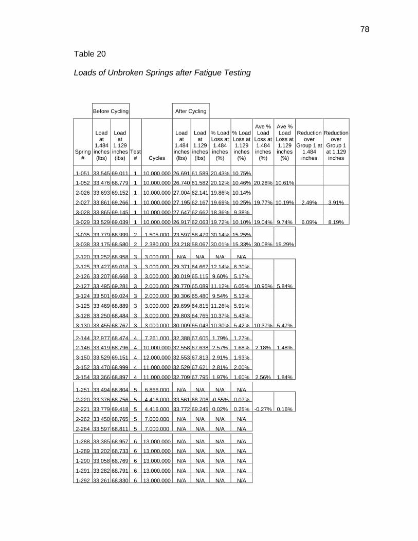
78
Table 20
Loads of Unbroken Springs after Fatigue Testing
Before Cycling
After Cycling
Spring #
Load at
1.484 inches (lbs)
Load at
1.129 inches (lbs)
Test # Cycles
Load at
1.484 inches (lbs)
Load at
1.129 inches (lbs)
% Load Loss at 1.484 inches
(%)
% Load Loss at 1.129 inches
(%)
Ave % Load
Loss at 1.484 inches
(%)
Ave % Load
Loss at 1.129 inches
(%)
Reduction over
Group 1 at 1.484 inches
Reduction over
Group 1 at 1.129 inches
1-051 33.545 69.011 1 10,000,000 26.691 61.589 20.43% 10.75%
1-052 33.476 68.779 1 10,000,000 26.740 61.582 20.12% 10.46% 20.28% 10.61%
2-026 33.693 69.152 1 10,000,000 27.004 62.141 19.86% 10.14%
2-027 33.861 69.266 1 10,000,000 27.195 62.167 19.69% 10.25% 19.77% 10.19% 2.49% 3.91%
3-028 33.865 69.145 1 10,000,000 27.647 62.662 18.36% 9.38%
3-029 33.529 69.039 1 10,000,000 26.917 62.063 19.72% 10.10% 19.04% 9.74% 6.09% 8.19%
3-035 33.779 68.999 2 1,505,000 23.597 58.479 30.14% 15.25%
3-038 33.175 68.580 2 2,380,000 23.218 58.067 30.01% 15.33% 30.08% 15.29%
2-120 33.252 68.958 3 3,000,000 N/A N/A N/A N/A
2-125 33.427 69.018 3 3,000,000 29.371 64.667 12.14% 6.30%
2-126 33.207 68.668 3 3,000,000 30.019 65.115 9.60% 5.17%
2-127 33.495 69.281 3 2,000,000 29.770 65.089 11.12% 6.05% 10.95% 5.84%
3-124 33.501 69.024 3 2,000,000 30.306 65.480 9.54% 5.13%
3-125 33.469 68.889 3 3,000,000 29.699 64.815 11.26% 5.91%
3-128 33.250 68.484 3 3,000,000 29.803 64.765 10.37% 5.43%
3-130 33.455 68.767 3 3,000,000 30.009 65.043 10.30% 5.42% 10.37% 5.47%
2-144 32.977 68.474 4 7,261,000 32.388 67.605 1.79% 1.27%
2-146 33.419 68.796 4 10,000,000 32.558 67.638 2.57% 1.68% 2.18% 1.48%
3-150 33.529 69.151 4 12,000,000 32.553 67.813 2.91% 1.93%
3-152 33.470 68.999 4 11,000,000 32.529 67.621 2.81% 2.00%
3-154 33.366 68.897 4 11,000,000 32.709 67.795 1.97% 1.60% 2.56% 1.84%
1-251 33.494 68.804 5 6,866,000 N/A N/A N/A N/A
2-220 33.376 68.756 5 4,416,000 33.561 68.706 -0.55% 0.07%
2-221 33.779 69.418 5 4,416,000 33.772 69.245 0.02% 0.25% -0.27% 0.16%
2-262 33.450 68.765 5 7,000,000 N/A N/A N/A N/A
2-264 33.597 68.811 5 7,000,000 N/A N/A N/A N/A
1-288 33.385 68.957 6 13,000,000 N/A N/A N/A N/A
1-289 33.202 68.733 6 13,000,000 N/A N/A N/A N/A
1-290 33.058 68.769 6 13,000,000 N/A N/A N/A N/A
1-291 33.282 68.791 6 13,000,000 N/A N/A N/A N/A
1-292 33.261 68.830 6 13,000,000 N/A N/A N/A N/A

79
1-293 33.519 68.984 6 13,000,000 N/A N/A N/A N/A
1-294 33.051 68.389 6 13,000,000 N/A N/A N/A N/A
1-295 33.023 68.481 6 13,000,000 N/A N/A N/A N/A
1-296 33.066 68.329 6 13,000,000 N/A N/A N/A N/A
2-266 33.297 68.739 6 13,000,000 33.566 69.026 -0.81% -0.42%
2-267 33.161 68.720 6 13,000,000 33.556 69.106 -1.19% -0.56%
2-268 33.387 68.907 6 13,000,000 33.525 69.122 -0.41% -0.31%
2-269 33.230 68.575 6 13,000,000 33.353 68.737 -0.37% -0.24%
2-270 33.226 68.365 6 13,000,000 33.224 68.501 0.01% -0.20%
2-271 33.535 69.109 6 13,000,000 33.835 69.329 -0.90% -0.32% -0.61% -0.34%
2-272 33.358 68.543 6 13,000,000 N/A N/A N/A N/A
2-274 33.150 68.405 6 13,000,000 N/A N/A N/A N/A
2-275 33.146 68.500 6 13,000,000 N/A N/A N/A N/A
Percent Load Loss Test (Stress Relaxation Test)
The results of the percent load loss test are shown in Figures 19-26.
There was no reduction of Percent Load Loss (Stress Relaxation) for the Group 3
springs (Stress Relieved at 700°F [371°C] for 1 hour, Cryogenically Treated,
Tempered at 300°F [149°C] for 2 hours) compared to the Group 1 springs (Stress
Relieved at 700°F [371°C] for 1 hour). This research indicates no benefit of
cryogenic treatment on the stress relaxation of the springs.
Figure 19 shows all three treatment groups of the same stress level (50
ksi, 90 ksi, and 130 ksi) very close together with a good straight line fit. Figures
20-26 are very similar.

80
Figure 19. Percent Load Loss Test: 250°F (121°C), 1.484 in. (37.7 mm) Spring Height.
0%
2%
4%
6%
8%
10%
12%
14%
16%
18%
20%
1 10 100 1000
Perc
en
t L
oad
Lo
ss
Hours
Percent Load Loss Test, 250°F (121°C) Measured at 1.484 in Spring Height
Group 1, 130 ksiGroup 1, 90 ksiGroup 1, 50 ksiGroup 2, 130 ksiGroup 2, 90 ksiGroup 2, 50 ksiGroup 3, 130 ksiGroup 3, 90 ksiGroup 3, 50 ksiLog. (Group 1, 130 ksi)Log. (Group 1, 90 ksi)Log. (Group 1, 50 ksi)Log. (Group 2, 130 ksi)Log. (Group 2, 90 ksi)Log. (Group 2, 50 ksi)Log. (Group 3, 130 ksi)Log. (Group 3, 90 ksi)Log. (Group 3, 50 ksi)
Group 1 = Stress Relieved at 700°F for 1 hr. (Green) Group 2 = Stress Relieved at 700°F for 1 hr, Tempered at 300°F for 2 hrs. (Red) Group 3 = Stress Relieved at 700°F for 1 hr, Cryogenically treated, Tempered at 300°F for 2 hrs. (Blue)

81
Figure 20. Percent Load Loss Test, 250°F (121°C), 1.129 in. (28.7 mm) Spring Height.
0%
1%
2%
3%
4%
5%
6%
7%
8%
9%
10%
1 10 100 1000
Perc
en
t L
oad
Lo
ss
Hours
Percent Load Loss Test, 250°F (121°C) Measured at 1.129 in Spring Height
Group 1, 130 ksiGroup 1, 90 ksiGroup 1, 50 ksiGroup 2, 130 ksiGroup 2, 90 ksiGroup 2, 50 ksiGroup 3, 130 ksiGroup 3, 90 ksiGroup 3, 50 ksiLog. (Group 1, 130 ksi)Log. (Group 1, 90 ksi)Log. (Group 1, 50 ksi)Log. (Group 2, 130 ksi)Log. (Group 2, 90 ksi)Log. (Group 2, 50 ksi)Log. (Group 3, 130 ksi)Log. (Group 3, 90 ksi)Log. (Group 3, 50 ksi)
Group 1 = Stress Relieved at 700°F for 1 hr. (Green) Group 2 = Stress Relieved at 700°F for 1 hr, Tempered at 300°F for 2 hrs. (Red) Group 3 = Stress Relieved at 700°F for 1 hr, Cryogenically treated, Tempered at 300°F for 2 hrs. (Blue)

82
Figure 21. Percent Load Loss Test, 350°F (177°C), 1.484 in. (37.7 mm) Spring Height.
0%
2%
4%
6%
8%
10%
12%
14%
16%
18%
20%
22%
24%
26%
1 10 100 1000
Perc
en
t L
oad
Lo
ss
Hours
Percent Load Loss Test, 350°F (177°C) Measured at 1.484 in Spring Height
Group 1, 130 ksiGroup 1, 90 ksiGroup 1, 50 ksiGroup 2, 130 ksiGroup 2, 90 ksiGroup 2, 50 ksiGroup 3, 130 ksiGroup 3, 90 ksiGroup 3, 50 ksiLog. (Group 1, 130 ksi)Log. (Group 1, 90 ksi)Log. (Group 1, 50 ksi)Log. (Group 2, 130 ksi)Log. (Group 2, 90 ksi)Log. (Group 2, 50 ksi)Log. (Group 3, 130 ksi)Log. (Group 3, 90 ksi)Log. (Group 3, 50 ksi)
Group 1 = Stress Relieved at 700°F for 1 hr. (Green) Group 2 = Stress Relieved at 700°F for 1 hr, Tempered at 300°F for 2 hrs. (Red) Group 3 = Stress Relieved at 700°F for 1 hr, Cryogenically treated, Tempered at 300°F for 2 hrs. (Blue)

83
Figure 22. Percent Load Loss Test, 350°F (177°C), 1.129 in. (28.7 mm) Spring Height.
0%
2%
4%
6%
8%
10%
12%
14%
1 10 100 1000
Perc
en
t L
oad
Lo
ss
Hours
Percent Load Loss Test, 350°F (177°C) Measured at 1.129 in Spring Height
Group 1, 130 ksiGroup 1, 90 ksiGroup 1, 50 ksiGroup 2, 130 ksiGroup 2, 90 ksiGroup 2, 50 ksiGroup 3, 130 ksiGroup 3, 90 ksiGroup 3, 50 ksiLog. (Group 1, 130 ksi)Log. (Group 1, 90 ksi)Log. (Group 1, 50 ksi)Log. (Group 2, 130 ksi)Log. (Group 2, 90 ksi)Log. (Group 2, 50 ksi)Log. (Group 3, 130 ksi)Log. (Group 3, 90 ksi)Log. (Group 3, 50 ksi)
Group 1 = Stress Relieved at 700°F for 1 hr. (Green) Group 2 = Stress Relieved at 700°F for 1 hr, Tempered at 300°F for 2 hrs. (Red) Group 3 = Stress Relieved at 700°F for 1 hr, Cryogenically treated, Tempered at 300°F for 2 hrs. (Blue)

84
Figure 23. Percent Load Loss Test, 450°F (232°C), 1.484 in. (37.7 mm) Spring Height.
0%
5%
10%
15%
20%
25%
30%
35%
40%
45%
1 10 100 1000
Perc
en
t L
oad
Lo
ss
Hours
Percent Load Loss Test, 450°F (232°C) Measured at 1.484 in Spring Height
Group 1, 130 ksiGroup 1, 90 ksiGroup 1, 50 ksiGroup 2, 130 ksiGroup 2, 90 ksiGroup 2, 50 ksiGroup 3, 130 ksiGroup 3, 90 ksiGroup 3, 50 ksiLog. (Group 1, 130 ksi)Log. (Group 1, 90 ksi)Log. (Group 1, 50 ksi)Log. (Group 2, 130 ksi)Log. (Group 2, 90 ksi)Log. (Group 2, 50 ksi)Log. (Group 3, 130 ksi)Log. (Group 3, 90 ksi)Log. (Group 3, 50 ksi)
Group 1 = Stress Relieved at 700°F for 1 hr. (Green) Group 2 = Stress Relieved at 700°F for 1 hr, Tempered at 300°F for 2 hrs. (Red) Group 3 = Stress Relieved at 700°F for 1 hr, Cryogenically treated, Tempered at 300°F for 2 hrs. (Blue)

85
Figure 24. Percent Load Loss Test, 450°F (232°C), 1.129 in. (28.7 mm) Spring Height.
0%
5%
10%
15%
20%
25%
1 10 100 1000
Perc
en
t L
oad
Lo
ss
Hours
Percent Load Loss Test, 450°F (232°C) Measured at 1.129 in Spring Height
Group 1, 130 ksiGroup 1, 90 ksiGroup 1, 50 ksiGroup 2, 130 ksiGroup 2, 90 ksiGroup 2, 50 ksiGroup 3, 130 ksiGroup 3, 90 ksiGroup 3, 50 ksiLog. (Group 1, 130 ksi)Log. (Group 1, 90 ksi)Log. (Group 1, 50 ksi)Log. (Group 2, 130 ksi)Log. (Group 2, 90 ksi)Log. (Group 2, 50 ksi)Log. (Group 3, 130 ksi)Log. (Group 3, 90 ksi)Log. (Group 3, 50 ksi)
Group 1 = Stress Relieved at 700°F for 1 hr. (Green) Group 2 = Stress Relieved at 700°F for 1 hr, Tempered at 300°F for 2 hrs. (Red) Group 3 = Stress Relieved at 700°F for 1 hr, Cryogenically treated, Tempered at 300°F for 2 hrs. (Blue)

86
Figure 25. Percent Load Loss Test, 550°F (288°C), 1.484 in. (37.7 mm) Spring Height.
0%
10%
20%
30%
40%
50%
60%
70%
80%
90%
1 10 100 1000
Perc
en
t L
oad
Lo
ss
Hours
Percent Load Loss Test, 550°F (288°C) Measured at 1.484 in Spring Height
Group 1, 130 ksiGroup 1, 90 ksiGroup 1, 50 ksiGroup 2, 130 ksiGroup 2, 90 ksiGroup 2, 50 ksiGroup 3, 130 ksiGroup 3, 90 ksiGroup 3, 50 ksiLog. (Group 1, 130 ksi)Log. (Group 1, 90 ksi)Log. (Group 1, 50 ksi)Log. (Group 2, 130 ksi)Log. (Group 2, 90 ksi)Log. (Group 2, 50 ksi)Log. (Group 3, 130 ksi)Log. (Group 3, 90 ksi)Log. (Group 3, 50 ksi)
Group 1 = Stress Relieved at 700°F for 1 hr. (Green) Group 2 = Stress Relieved at 700°F for 1 hr, Tempered at 300°F for 2 hrs. (Red) Group 3 = Stress Relieved at 700°F for 1 hr, Cryogenically treated, Tempered at 300°F for 2 hrs. (Blue)

87
Figure 26 .Percent Load Loss Test, 550°F (288°C), 1.129 in. (28.7 mm) Spring Height.
0%
5%
10%
15%
20%
25%
30%
35%
40%
45%
50%
1 10 100 1000
Perc
en
t L
oad
Lo
ss
Hours
Percent Load Loss Test, 550°F (288°C) Measured at 1.129 in Spring Height
Group 1, 130 ksi
Group 1, 90 ksi
Group 1, 50 ksi
Group 2, 130 ksi
Group 2, 90 ksi
Group 2, 50 ksi
Group 3, 130 ksi
Group 3, 90 ksi
Group 3, 50 ksi
Log. (Group 1, 130 ksi)
Log. (Group 1, 90 ksi)
Log. (Group 1, 50 ksi)
Log. (Group 2, 130 ksi)
Log. (Group 2, 90 ksi)
Log. (Group 2, 50 ksi)
Log. (Group 3, 130 ksi)
Log. (Group 3, 90 ksi)
Log. (Group 3, 50 ksi)
Group 1 = Stress Relieved at 700°F for 1 hr. (Green) Group 2 = Stress Relieved at 700°F for 1 hr, Tempered at 300°F for 2 hrs. (Red) Group 3 = Stress Relieved at 700°F for 1 hr, Cryogenically treated, Tempered at 300°F for 2 hrs. (Blue)

88
Fatigue Tests
Six fatigue tests were performed at varying Mean Shear Stress and
Amplitude Stress, to achieve Equivalent Fully Reversed Shear Stresses between
76,611 psi and 184,930 psi (528 MPa and 1275 MPa). Refer to Table 21 for a
comparison.
Table 21
Table Comparing Fatigue Tests 1-6.
Goodman Safety Factor
Mean Shear Stress
Amplitude Shear Stress
Equivalent Fully Reversed Shear
Stress
Frequency, Hz
Fatigue Test 1 0.922 147,300 psi
1,015 MPa
16,500 psi
114 MPa
78,300 psi
540 MPa
7
Fatigue Test 2 0.568 121,100 psi *
835 MPa
65,000 psi **
448 MPa
184,900 psi ***
1,275 MPa
7
Fatigue Test 3 0.614 110,700 psi
763 MPa
58,000 psi
400 MPa
142,300 psi
981 MPa
10
Fatigue Test 4 0.669 85,900 psi
592 MPa
58,000 psi
400 MPa
107,300 psi
740 MPa
10
Fatigue Test 5 0.711 69,300 psi
478 MPa
58,000 psi
400 MPa
92,100 psi
635 MPa
10
Fatigue Test 6 0.834 85,900 psi
592 MPa
41,400 psi
285 MPa
76,600 psi
528 MPa
10
* Reduced from 136,000 psi due to yielding.
** Increased from 58,000 psi due to yielding.
*** Reduced from 211,240 psi due to yielding.

89
The Fatigue Test load points were shown on a Haigh Diagram in Figure
27. Load points below the Goodman Line would be expected to have infinite life.
The further above and to the right of the Goodman Line, the smaller the
Goodman Safety Factor. Load points above and to the right of the Yield Line
would be expected to yield.
Figure 27. Haigh Diagram of Fatigue Tests 1-6.
0
50,000
100,000
150,000
200,000
0 50,000 100,000 150,000 200,000
τ a (p
si)
τm (psi)
Haigh Diagram
Goodman LineYield LineSsaFatigue Test 1, Goodman SF = 0.922Fatigue Test 2, Goodman SF = 0.568Fatigue Test 3, Goodman SF = 0.614Fatigue Test 4, Goodman SF = 0.669Fatigue Test 5, Goodman SF = 0.711Fatigue Test 6, Goodman SF = 0.834
Sse: Fully Reversed Endurance Strength
Ssa: Fully Reversed Endurance Amplitude
Ssu: Ultimate Shear Strength
Ssy: Torsional Yield Strength

90
The results of Fatigue Tests 1-6 are shown in Tables 22-27. Fatigue Test
1 was stopped after 6 springs (two from each treatment group) ran 10 million
cycles without any failures. Nine Group 1 springs and nine Group 2 springs ran
13 million cycles during Fatigue Test 6 without failing. Group 3 springs were not
included in Fatigue Tests 5 or 6 because the number of cycles to failure in
Fatigue Test 4 were so high, and three springs did not break at 11 million cycles
and above.
Table 22
Fatigue Test 1 Data.
Spring Height Range (inches): 1.03 - 0.83
Force Range (pounds): 78.70 - 98.62
Mean Load (pounds): 88.66
Amplitude Load (pounds): 9.96
Mean Shear Stress (psi): 147,282
Amplitude Shear Stress (psi): 16,549
Equivalent Fully Reversed Shear Stress (psi), i.e. R = -1 78,289
Frequency (Hz) 7
Goodman Safety Factor 0.922
Group 1: Stress Relieved at 700ºF (371°C) for 1
hour.
Group 2: Stress Relieved at 700ºF (371°C) for 1 hour,
Tempered at 300ºF (149°C) for 2 hours.
Group 3: Stress Relieved at 700ºF (371°C) for 1 hour,
Cryogenically Treated, Tempered at 300ºF (149°C)
for 2 hours.
Sample Number Cycles to Break Number Cycles to Break Number Cycles to Break
1 1-051
not broke 10,000,000 2-026
not broke 10,000,000 3-028
not broke 10,000,000
2 1-052
not broke 10,000,000 2-027
not broke 10,000,000 3-029
not broke 10,000,000

91
Table 23
Fatigue Test 2 Data
Spring Height Range (inches): 1.35 - 0.65
Force Range (pounds): 46.69 - 116.47
Mean Load (pounds): 81.58
Amplitude Load (pounds): 34.89
Mean Shear Stress (psi): 121,149 (was 135,524)
Amplitude Shear Stress (psi): 64,968 (was 57,952)
Equivalent Fully Reversed Shear Stress (psi),
i.e. R = -1 184,930 (was 211,240)
Frequency (Hz) 7
Goodman Safety Factor 0.568
Group 1: Stress Relieved at 700ºF (371°C) for 1 hour.
Group 2: Stress Relieved at 700ºF (371°C) for 1
hour, Tempered at 300ºF (149°C) for 2 hours.
Group 3: Stress Relieved at 700ºF (371°C) for 1 hour,
Cryogenically Treated, Tempered at 300ºF (149°C)
for 2 hours.
Sample Number Cycles to Break Number Cycles to Break Number Cycles to Break
1 1-068 71,000 2-033 95,000 3-036 60,000
2 1-065 78,000 2-039 140,000 3-045 75,000
3 1-066 104,000 2-041 225,000 3-039 80,000
4 1-057 120,000 2-043 228,000 3-042 80,000
5 1-064 176,000 2-036 260,000 3-037 85,000
6 1-059 231,000 2-040 300,000 3-043 105,000
7 1-060 273,000 2-042 300,000 3-041 165,000
8 1-062 333,000 2-032 472,000 3-040 305,000
9 1-067 336,000 2-037 525,000 3-044 335,000
10 1-063 367,000 2-038 535,000 3-034 622,000
11 1-058 381,000 2-035 735,000 3-035 not broke 1,505,000
12 1-061 399,000 2-034 1,890,000 3-038 not broke 2,380,000
Distribution Weibull-2Parameter Weibull-2Parameter Weibull-2Parameter
Analysis
MLE/SRM (maximum likelihood/Standard Regression Method)
MLE/SRM (maximum likelihood/Standard Regression Method)
MLE/SRM (maximum likelihood/Standard Regression Method)
CB (Confidence Bound) Method FM (Fischer Matrix) FM (Fischer Matrix) FM (Fischer Matrix)
Ranking MED (Median Ranks) MED (Median Ranks) MED (Median Ranks)
Beta (slope of line) 2.136 1.225 0.656
Eta (Characteristic Life) 270,564 513,664 483,605
LK (Logarithmic Likelihood) Value -157 -169 -141
Failures \ Suspensions 12 \ 0 12 \ 0 10 \ 2

92
Table 24
Fatigue Test 3 Data
Spring Height Range (inches): 1.50 - 0.80
Force Range (pounds): 31.74 - 101.52
Mean Load (pounds): 66.63
Amplitude Load (pounds): 34.89
Mean Shear Stress (psi): 110,688
Amplitude Shear Stress (psi): 57,952
Equivalent Fully Reversed Shear Stress (psi),
i.e. R = -1 142,275
Frequency (Hz) 10
Goodman Safety Factor 0.614
Group 1: Stress Relieved at 700ºF (371°C) for 1
hour.
Group 2: Stress Relieved at 700ºF (371°C) for 1 hour,
Tempered at 300ºF (149°C) for 2 hours.
Group 3: Stress Relieved at 700ºF (371°C) for 1
hour, Cryogenically Treated, Tempered at
300ºF (149°C) for 2 hours.
Sample Number Cycles to Break Number Cycles to Break Number Cycles to Break
1 1-149 157,000 2-119 130,000 3-122 67,000
2 1-154 176,000 2-123 252,000 3-127 88,000
3 1-152 290,000 2-124 482,000 3-126 127,000
4 1-153 300,000 2-122 532,000 3-121 132,000
5 1-156 300,000 2-121 756,000 3-123 134,000
6 1-150 531,000 2-128 984,000 3-129 2,000,000
7 1-151 610,000 2-127
not broke 2,000,000 3-124
not broke 2,000,000
8 1-147 816,000 2-120
not broke 3,000,000 3-125
not broke 3,000,000
9 1-155 1,100,000 2-125
not broke 3,000,000 3-128
not broke 3,000,000
10 1-148 1,683,000 2-126
not broke 3,000,000 3-130
not broke 3,000,000
Distribution Weibull-2Parameter Weibull-2Parameter Weibull-2Parameter
Analysis
MLE/SRM (maximum likelihood/Standard Regression Method)
MLE/SRM (maximum likelihood/Standard Regression Method)
MLE/SRM (maximum likelihood/Standard Regression Method)
CB (Confidence Bound) Method FM (Fischer Matrix) FM (Fischer Matrix) FM (Fischer Matrix)
Ranking MED (Median Ranks) MED (Median Ranks) MED (Median Ranks)
Beta (slope of line) 1.396 0.724 0.470
Eta (Characteristic Life) 659,445 2,582,300 2,690,115
LK (Logarithmic Likelihood) Value -143 -94 -91
Failures \ Suspensions 10 \ 0 6 \ 4 6 \ 4

93
Table 25
Fatigue Test 4 Data
Spring Height Range (inches): 1.65 - 0.95
Force Range (pounds): 16.79 - 86.57
Mean Load (pounds): 51.68
Amplitude Load (pounds): 34.89
Mean Shear Stress (psi): 85,851
Amplitude Shear Stress (psi): 57,952
Equivalent Fully Reversed Shear Stress
(psi), i.e. R = -1 107,256
Frequency (Hz) 10
Goodman Safety Factor 0.669
Group 1: Stress Relieved at 700ºF (371°C) for 1
hour.
Group 2: Stress Relieved at 700ºF (371°C) for 1 hour,
Tempered at 300ºF (149°C) for 2 hours.
Group 3: Stress Relieved at 700ºF (371°C) for 1
hour, Cryogenically Treated, Tempered at
300ºF (149°C) for 2 hours.
Sample Number Cycles to Break Number Cycles to Break Number Cycles to Break
1 1-175 200,000 2-147 99,000 3-155 121,000
2 1-181 270,000 2-153 258,000 3-151 132,000
3 1-178 405,000 2-149 298,000 3-153 389,000
4 1-174 495,000 2-148 444,000 3-146 1,624,000
5 1-180 911,000 2-151 1,838,000 3-149 6,200,000
6 1-173 1,092,000 2-152 2,476,000 3-147 7,421,000
7 1-179 1,216,000 2-145 3,237,000 3-148 9,101,000
8 1-172 1,372,000 2-150 4,046,000 3-152
not broke 11,000,000
9 1-177 1,377,000 2-144 not broke 7,261,000 3-154
not broke 11,000,000
10 1-176 2,000,086 2-146
not broke 10,000,000 3-150
not broke 12,000,000
Distribution Weibull-2Parameter Weibull-2Parameter Weibull-2Parameter
Analysis
MLE/SRM (maximum likelihood/Standard Regression Method)
MLE/SRM (maximum likelihood/Standard Regression Method)
MLE/SRM (maximum likelihood/Standard Regression Method)
CB (Confidence Bound) Method FM (Fischer Matrix) FM (Fischer Matrix) FM (Fischer Matrix)
Ranking MED (Median Ranks) MED (Median Ranks) MED (Median Ranks)
Beta (slope of line) 1.721 0.646 0.569
Eta (Characteristic Life) 1,048,330 3,388,017 8,669,896
LK (Logarithmic Likelihood) Value -146 -128 -117
Failures \ Suspensions 10 \ 0 8 \ 2 7 \ 3

94
Table 26
Fatigue Test 5 Data
Spring Height Range (inches): 1.75 - 1.05
Force Range (pounds): 6.83 - 76.60
Mean Load (pounds): 41.72
Amplitude Load (pounds): 34.89
Mean Shear Stress (psi): 69,294
Amplitude Shear Stress (psi): 57,952
Equivalent Fully Reversed Shear Stress (psi), i.e. R = -1 92,138
Frequency (Hz) 10
Goodman Safety Factor 0.711
Group 1: Stress Relieved at 700ºF (371°C) for 1 hour.
Group 2: Stress Relieved at 700ºF (371°C) for 1 hour,
Tempered at 300ºF (149°C) for 2 hours.
Group 3: Stress Relieved at 700ºF (371°C) for 1
hour, Cryogenically Treated, Tempered at
300ºF (149°C) for 2 hours.
Sample Number Cycles to Break Number Cycles to Break Number Cycles to Break
1 1-249 217,000 2-215 72,000 N/A N/A
2 1-243 245,000 2-217 87,000 N/A N/A
3 1-245 1,073,000 2-218 178,000 N/A N/A
4 1-242 1,201,000 2-222 285,000 N/A N/A
5 1-247 1,216,000 2-223 322,000 N/A N/A
6 1-248 1,256,000 2-261 1,000,000 N/A N/A
7 1-244 1,917,000 2-214 2,426,000 N/A N/A
8 1-246 3,871,000 2-216 3,031,000 N/A N/A
9 1-250 5,841,000 2-265 3,310,000 N/A N/A
10 1-251
not broke 6,866,000 2-219 3,617,000 N/A N/A
11 N/A N/A 2-260 4,312,000 N/A N/A
12 N/A N/A 2-263 4,773,000 N/A N/A
13 N/A N/A 2-220 not broke 4,416,000 N/A N/A
14 N/A N/A 2-221 not broke 4,416,000 N/A N/A
15 N/A N/A 2-262 not broke 7,000,000 N/A N/A
16 N/A N/A 2-264 not broke 7,000,000 N/A N/A
Distribution Weibull-2Parameter Weibull-2Parameter
Analysis
MLE/SRM (maximum likelihood/Standard Regression Method)
MLE/SRM (maximum likelihood/Standard Regression Method)
CB (Confidence Bound) Method FM (Fischer Matrix) FM (Fischer Matrix) Ranking MED (Median Ranks) MED (Median Ranks) Beta (slope of line) 0.938 0.693 Eta (Characteristic Life) 2,584,452 3,799,701 LK (Logarithmic Likelihood) Value -142 -193 Failures \ Suspensions 9 \ 1 12 \ 4

95
Table 27
Fatigue Test 6 Data
Spring Height Range (inches): 1.55 - 1.05
Force Range (pounds): 26.76 - 76.60
Mean Load (pounds): 51.68
Amplitude Load (pounds): 24.92
Mean Shear Stress (psi): 85,851
Amplitude Shear Stress (psi): 41,374
Equivalent Fully Reversed Shear Stress (psi), i.e. R = -1 76,611
Frequency (Hz) 10
Goodman Safety Factor 0.834
Group 1: Stress Relieved at 700ºF (371°C) for 1 hour.
Group 2: Stress Relieved at 700ºF (371°C) for 1 hour,
Tempered at 300ºF (149°C) for 2 hours.
Group 3: Stress Relieved at 700ºF (371°C) for 1
hour, Cryogenically Treated, Tempered at
300ºF (149°C) for 2 hours.
Sample Number Cycles to Break Number Cycles to Break Number Cycles to Break
1 1-288
not broke 13,000,000 2-266
not broke 13,000,000 N/A N/A
2 1-289
not broke 13,000,000 2-267
not broke 13,000,000 N/A N/A
3 1-290
not broke 13,000,000 2-268
not broke 13,000,000 N/A N/A
4 1-291
not broke 13,000,000 2-269
not broke 13,000,000 N/A N/A
5 1-292
not broke 13,000,000 2-270
not broke 13,000,000 N/A N/A
6 1-293
not broke 13,000,000 2-271
not broke 13,000,000 N/A N/A
7 1-294
not broke 13,000,000 2-272
not broke 13,000,000 N/A N/A
8 1-295
not broke 13,000,000 2-274
not broke 13,000,000 N/A N/A
9 1-296
not broke 13,000,000 2-275
not broke 13,000,000 N/A N/A
Weibull plots were used for each fatigue test (Fatigue Test 2-Fatigue Test
5). Refer to Figures 28-31. The Weibull plot shows the data points of the failures
and a straight line fit to the data, all on a specialized paper grid. The further to
the right the straight line is, the greater the number of cycles at failure. The
steeper the slope of the line, β, the smaller the spread of the data. A vertical line

96
could be interpreted that all of the samples failed at exactly the same number of
cycles. So, the desired straight line fit would be a nearly vertical line as far to the
right as possible.
In some tests, failures did not occur. These are shown as suspended
points along the horizontal axis of the plot. The values of these suspended
points was used in the calculation of the straight line.
The LK (Logarithmic Likelihood) Value is a measure of how well the
straight line fits the data points. The less negative the LK Value, the better the fit.
In Fatigue Tests 2, 3, and 4, the Group 3 Springs (Stress Relieved at 700°F
[371°C] for 1 hour, Cryogenically Treated, Tempered at 300°F [149°C] for 2
hours) had better fits than the Group 1 (Stress Relieved at 700°F [371°C] for 1
hour) and Group 2 Springs (Stress Relieved at 700°F [371°C] for 1 hour,
Tempered at 300°F [149°C] for 2 hours).
In Fatigue Tests 2,3, and 4 (Figures 28-30) it appears that the Group 3
Springs (Stress Relieved at 700°F [371°C] for 1 hour, Cryogenically Treated,
Tempered at 300°F [149°C] for 2 hours) follow more of an S-shape than a
straight line fit. This can be referred to as a “mixed Weibull distribution” or a
“multimodal Weibull.” This would imply more than one failure mode.
("Weibull++7", p. 333) Since multiple failure modes is not the case for this
research, it is believed that additional data points would smooth out the fit to the
straight line.

97
Figure 28. Fatigue Test 2: 135.52 ksi mean stress, 57.95 ksi amplitude stress.

98
Figure 29. Fatigue Test 3: 110.69 ksi mean stress, 57.95 ksi amplitude stress.

99
Figure 30. Fatigue Test 4: 85.85 ksi, mean stress, 57.96 ksi amplitude stress.

100
Figure 31. Fatigue Test 5: 69.29 ksi mean stress, 57.95 ksi amplitude stress.
Refer to Table 28 and Figures 32-39 for results, bar charts and S-N
diagrams.
Data from the Weibull plots can be extracted for use in the S-N Diagrams. The B10 Life is the number of cycles where the curve crosses the 10.0 Unreliability. This is "the number of cycles where 10% of the population are estimated to fail." Bearing manufacturers like to use this value.
The B50 Life is the number of cycles where the curve crosses the 50.0 Unreliability. This is "the number of cycles where 50% of the population are estimated to fail."
The Characteristic Life is the number of cycles where the curve crosses the 63.2 Unreliability. This is "the number of cycles

101
where 63.2% of the population are estimated to fail." The Reliasoft Weibull software calculates and prints this value on the bottom of the charts, assigned to the Greek letter eta.
The B90 Life is the number of cycles where the curve crosses the 90.0 Unreliability. This is "the number of cycles where 90% of the population are estimated to fail." (Society of Automotive Engineers, 1997, p. 72)

102
Table 28
Fatigue Test 2 – Fatigue Test 5 Data
Fatigue Test
Number
Calculated Fully
Reversed Load, psi
Group 1: Stress
Relieved at 700ºF
(371°C) for 1 hour.
Group 2: Stress
Relieved at 700ºF
(371°C) for 1 hour,
Tempered at 300ºF
(149°C) for 2 hours.
Group 3: Stress
Relieved at 700ºF
(371°C) for 1 hour,
Cryogenically Treated,
Tempered at 300ºF
(149°C) for 2 hours.
Percent Increase of
Group 3 over Group 1
Percent Increase of
Group 2 over Group 1
B90 (90% Unreliability)
5 92,138 6,289,975 12,650,920 N/A N/A 101%
4 107,256 1,702,535 12,315,280 37,550,950 2106% 623%
3 142,275 1,198,526 8,177,681 15,882,780 1225% 582%
2 184,930 399,836 1,014,468 1,723,682 331% 154%
Characteristic Life (63.2% Unreliability)
5 92,138 2,584,452 3,799,701 N/A N/A 47%
4 107,256 1,048,330 3,388,017 8,669,896 727% 223%
3 142,275 659,445 2,582,299 2,690,115 308% 292%
2 184,930 270,564 513,664 483,605 79% 90%
B50 (50% Unreliability) 5 92,138 1,747,829 2,238,815 N/A N/A 28%
4 107,256 847,178 1,921,627 4,552,843 437% 127%
3 142,275 507,148 1,555,861 1,232,899 143% 207%
2 184,930 227,918 380,904 276,728 21% 67%
B10 (10% Unreliability) 5 92,138 234,630 147,901 N/A N/A -37%
4 107,256 283,430 104,212 165,924 -41% -63%
3 142,275 131,522 115,177 22,355 -83% -12%
2 184,930 94,353 81,917 15,688 -83% -13%
The data from the table was put into bar charts showing the number of
cycles extracted from each of the Weibull plots for a certain stress level. Except
for the B10 Life Bar Chart, the Group 3 springs (Stress Relieved at 700°F [371°C]
for 1 hour, Cryogenically Treated, Tempered at 300°F [149°C] for 2 hours) had
higher cycles that the Group 1 springs (Stress Relieved at 700°F [371°C] for 1
hour, Cryogenically Treated, Tempered at 300°F [149°C] for 2 hours).

103
Figure 32. B90 Life Bar Chart
Figure 33. Characteristic Life Bar Chart.
0
5,000,000
10,000,000
15,000,000
20,000,000
25,000,000
30,000,000
35,000,000
40,000,000
92,138 107,256 142,275 184,930
Lif
e, cycle
s
Calculated Fully Reversed Load, psi
B90 Life (90% Unreliability) Bar Chart
Group 1
Group 2
Group 3
0
1,000,000
2,000,000
3,000,000
4,000,000
5,000,000
6,000,000
7,000,000
8,000,000
9,000,000
10,000,000
92,138 107,256 142,275 184,930
Lif
e,
cycle
s
Calculated Fully Reversed Load, psi
Characteristic Life (63.2% Unreliability) Bar Chart
Group 1
Group 2
Group 3
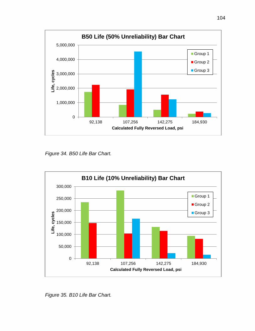
104
Figure 34. B50 Life Bar Chart.
Figure 35. B10 Life Bar Chart.
0
1,000,000
2,000,000
3,000,000
4,000,000
5,000,000
92,138 107,256 142,275 184,930
Lif
e,
cycle
s
Calculated Fully Reversed Load, psi
B50 Life (50% Unreliability) Bar Chart
Group 1
Group 2
Group 3
0
50,000
100,000
150,000
200,000
250,000
300,000
92,138 107,256 142,275 184,930
Lif
e, cycle
s
Calculated Fully Reversed Load, psi
B10 Life (10% Unreliability) Bar Chart
Group 1
Group 2
Group 3

105
The Group 3 springs had a longer cycle life at most stress levels than the
Group 1 springs. This could be seen in the figures below for B90 Life,
Characteristic Life (B63.2), and B50 Life. Only in the B10 Life did the Group 3
Springs exhibit a shorter life than Group 1 Springs.
Figure 36. S-N Diagram, B90 Life, MLE.
10,000
100,000
1,000,000
10,000 100,000 1,000,000 10,000,000 100,000,000
Eq
uiv
ale
nt
Fu
lly R
ev
ers
ed
Sh
ear
Str
ess,
psi
Cycles
S-N Diagram, B90 Life MLE
Group 1: Stress Relieved at 700F for 1 hr.
Group 2: Stress Relieved at 700F for 1 hr, Tempered at 300F for 2hrs. (qty 16 for 92k)
Group 3: Stress Relieved at 700F for 1 hr, Cryogenically Treated,Tempered at 300F for 2 hrs.
Not an actual Failure Point. Group 1: Nine springs did not fail after 13 million cycles. Group 2: Nine springs did not fail after 13 million cycles.

106
Figure 37. S-N Diagram Characteristic Life B63.2.
10,000
100,000
1,000,000
10,000 100,000 1,000,000 10,000,000 100,000,000
Eq
uiv
ale
nt
Fu
lly R
ev
ers
ed
Sh
ear
Str
ess,
psi
Cycles
S-N Diagram, Characteristic Life MLE [B63.2]
Group 1: Stress Relieved at 700F for 1 hr.
Group 2: Stress Relieved at 700F for 1 hr, Tempered at 300F for 2 hrs.(16 springs for 92k)
Group 3: Stress Relieved at 700F for 1 hr, Cryogenically Treated,Tempered at 300F for 2 hrs.
Not an actual Failure Point. Group 1: Nine springs did not fail after 13 million cycles. Group 2: Nine springs did not
fail after 13 million cycles.

107
Figure 38. S-N Diagram, B50 Life, MLE
10,000
100,000
1,000,000
10,000 100,000 1,000,000 10,000,000 100,000,000
Eq
uiv
ale
nt
Fu
lly R
ev
ers
ed
Sh
ear
Str
ess,
psi
Cycles
S-N Diagram, B50 Life MLE
Group 1: Stress Relieved at 700F for 1 hr.
Group 2: Stress Relieved at 700F for 1 hr, Tempered at 300F for 2hrs. (qty 16 at 92k)
Group 3: Stress Relieved at 700F for 1 hr, Cryogenically Treated,Tempered at 300F for 2 hrs.
Not an actual Failure Point. Group 1: Nine springs did not fail after 13 million cycles. Group 2: Nine springs did not fail after 13 million cycles.

108
.
Figure 39. S-N Diagram, B10 Life, MLE.
Refer to Table 29 for a comparison of estimated endurance limits. If a
spring was operated at a stress equal to or below the Endurance Limit infinite life
would be expected. It would typically be found at a bend in the curve of the S-N
Diagram, where the curve is more horizontal. The Group 3 springs (Stress
Relieved at 700°F [371°C] for 1 hour, Cryogenically Treated, Tempered at 300°F
[149°C] for 2 hours) exhibited a 25% increase in Estimated Endurance Limit,
80,000 psi (552 MPa) to 100,000 psi (689 MPa), compared to the Group 1
springs (Stress Relieved at 700°F [371°C] for 1 hour). In terms of percent of
10,000
100,000
1,000,000
10,000 100,000 1,000,000 10,000,000 100,000,000
Eq
uiv
ale
nt
Fu
lly R
ev
ers
ed
Sh
ear
Str
ess,
psi
Cycles
S-N Diagram, B10 Life MLE
Group 1: Stress Relieved at 700F for 1 hr.
Group 2: Stress Relieved at 700F for 1 hr, Tempered at 300F for 2hrs. (Qty 16 for 92k)
Group 3: Stress Relieved at 700F for 1 hr, Cryogenically Treated,Tempered at 300F for 2 hrs.
Not an actual Failure Point. Group 1: Nine springs did not fail after 13 million cycles. Group 2: Nine springs did not fail after 13 million cycles.

109
tensile strength, the Group 3 springs had an estimated endurance limit of 36% of
tensile strength, compared to Group 1 springs which had an estimated
endurance limit of 29% of tensile strength.
These results show higher improvements than resulted from Zhirafar‟s
fatigue testing of 4340 nickel-chromium-molybdenum steel R.R. Moore rotating
beam fatigue specimens, as discussed in the literature review.
Table 29
Estimated Endurance Limit
Estimated Endurance
Limit
Percent of
Tensile Strength
Group 1: Stress Relieved at 700°F
(371°C) for 1 hour.
80,000 psi
552 MPa
29%
Group 2: Stress Relieved at 700°F
(371°C) for 1 hour, Tempered at
300°F (149°C) for 2 hours.
80,000 psi
552 MPa
29%
Group 3: Stress Relieved at 700°F
(371°C) for 1 hour, Cryogenically
Treated, Tempered at 300°F (149°C)
for 2 hours.
100,000 psi
690 MPa
36%

110
Metallographic Tests
Microstructures
A Group 1 wire sample molded in epoxy, polished and etched in Nital, was
examined to look for retained austenite. No observable retained austenite could
be seen. A Group 2 wire sample molded in epoxy, polished and etched in Nital,
was examined to look for retained austenite. No observable retained austenite
could be seen. A Group 3 wire sample molded in epoxy, polished and etched in
Nital, was examined to look for retained austenite. No observable retained
austenite could be seen. All three structures looked the same. The photos
showed all tempered martensite, of fairly small lath size. The differences in
colors; tan, white, and gray, merely show the effect of the etchant on different
orientations of the martensite laths.
A Group 1 wire sample was austenitized at 1600°F (871°C) for 30
minutes, water quenched, and tempered 482°F (250°C) for one hour. It was
molded in epoxy, polished and etched in Nital. No observable retained austenite
could be seen. The photo showed all martensite, of larger grain size than the
Group 1, Group 2, or Group 3 microstructures. Refer to Figures 40-43.

111
Figure 40. Microstructure of Group 1.

112
Figure 41. Microstructure of Group 2.

113
Figure 42. Microstructure of Group 3.

114
Figure 43. Microstructure of modified Group 1 wire: Austenitized at 1600°F (871°C) for 30 minutes, water quenched, tempered at 482°F (250°C) for 1 hour.
Eta Carbides
The results of the eta carbides measurement are shown in Table 30. The
extracted material from sample 1-269 yielded 1.6 percent by weight of the
specimen. Given the broad hump at lower angles and general high background
throughout the pattern, it appears from an x-ray diffraction standpoint that the
material is amorphous.

115
The extracted material from sample 2-242 yielded a 1.3 percent by weight
of the specimen. The diffraction pattern was similar to that of 1-269.
The extracted material from sample 3-233 yielded 2.4 percent by weight of
the specimen. The diffraction pattern was similar to samples 1-269 and 2-242.
The diffraction patterns obtained from all three samples did not produce any
diffraction peaks and as such, is not believed to consist of much, if any carbides.
Table 30
Eta Carbides
Sample Extracted Material
Diffraction Peaks / Carbides
Group 1: Stress Relieved at 700°F (371°C) for 1 hour.
1-269 1.6% None / None
Group 2: Stress Relieved at 700°F (371°C) for 1 hour, Tempered at 300°F (149°C) for 2
hours.
2-242 1.3% None / None
Group 3: Stress Relieved at 700°F (371°C) for 1 hour, Cryogenically Treated, Tempered
at 300°F (149°C) for 2 hours.
3-233 2.4% None / None
See Appendix C for tables and quantitative phase analysis.
SEM of Fractured Surface
Photographs of the fractured surface of Sample 3-151 were taken using
the Scanning Electron Microscope, as shown in Figures 44-48.
116
The upper right quadrant (Figure 45) showed little black cracks, no
striations, no dimples, no cleavage. This was a fatigue region at the inside of the
coil.
The lower right quadrant (Figure 46) showed fine dimples. This was a
ductile fracture area.
The lower left quadrant (Figure 47) showed elongated dimples. This was
a ductile fracture area.
The upper left quadrant (Figure 48) showed cracking with no dimples.
This was a fatigue region at the inside of the coil.

117
Figure 44 .Sample 3-151 Low Magnification SEM.
Figure 45
Figure 46
Figure 48
Figure 47
Outside of coil.
Inside of coil.

118
Figure 45. Sample 3-151 High Magnification SEM Upper Right Quadrant.

119
Figure 46. Sample 3-151 High Magnification SEM Lower Right Quadrant.

120
Figure 47. Sample 3-151 High Magnification SEM Lower Left Quadrant.

121
Figure 48. Sample 3-151 High Magnification SEM, Upper Left Quadrant.

122
CHAPTER 5
CONCLUSIONS AND SUGGESTIONS
Conclusions
The Group 3 (Stress Relieved at 700°F [371°C] for 1 hour, Cryogenically
Treated, Tempered at 300°F [149°C] for 2 hours) springs have a longer cycle life
at most stress levels and a higher estimated endurance limit than the Group 1
(Stress Relieved at 700°F [371°C] for 1 hour) springs. The improved fatigue life
of cryogenically treated springs (Group 3) is due to an increase in the
compressive residual stress at the surface of the spring
There was no reduction of Percent Load Loss (Stress Relaxation) for the
Group 3 springs (Stress Relieved at 700°F [371°C] for 1 hour, Cryogenically
Treated, Tempered at 300°F [149°C] for 2 hours) compared to the Group 1
springs (Stress Relieved at 700°F [371°C] for 1 hour).
Suggestions for Further Study
Hardness. Further study is needed with many more samples to determine
if there is any improvement in due to cryogenic treatment.
Shot Peening. Since shot peening has been the fatigue improvement
treatment of choice for many years, a comparison of shot peening to cryogenic
treatment would be very interesting.

123
Cryogenic treatment down to the temperature of liquid helium. Newer
cryogenic chambers can actually achieve temperatures as low as liquid helium,
-452°F (-269°C), compared to liquid nitrogen, -305°F (-187°C). It would be
interesting to see how much additional fatigue life could be obtained with
treatments down to that temperature.
Austenitic stainless steel and music wire. Music wire and 302 stainless
steel are two very popular materials for compression springs. It would be
interesting to see if these materials exhibited similar improvements in fatigue life.

124
REFERENCES
ASTM International. (2003). Standard Specification for Steel Wire, Chromium-Silicon Alloy (A 401/A 401M-03). West Conshohocken, PA.
ASTM International. (2005). Standard Specification for Steel Wire, Chromium-Silicon Alloy Valve Spring Quality (A 877/A 877M-05). West Conshohocken, PA.
Averbach, B., & Cohen, M. (1948). Unknown title. Transactions of American Institute of Mining, Metallurgical, and Petroleum Engineers, 176, 401.
Barron, R. (1982). Cryogenic treatment of metals to improve wear resistance. Cryogenics, 22(8), 409-413.
Baumeister, T. (Ed.). (1978). Mark's Standard Handbook for Mechanical Engineers (8th ed.). New York: McGraw-Hill, Inc. (Original work published 1916)
Beuter, H. (2002). Handbook of Spring Design [Brochure]. Oak Brook, IL: Spring Manufacturers Institute, Inc.
Carlson, E. (1991). Cold Treating and Cryogenic Treatment of Steel. In Metals Handbook (10th ed., Vol. 4, pp. 203-206). Metals Park, OH: ASM International.
Cullity, B. (2001). Elements of X-Ray Diffraction (3rd ed.). Upper Saddle River, NJ: Prentice-Hall, Inc.
DeFord, R. (2006). The Importance of Spring Index. Springs, 45(1), 25-26.
DeFord, R. (2006). The Quick and Easy Material Review. Springs, 45(2), 47-48.
Deutschman, A. (1975). Machine Design Theory and Practice. New York: Macmillan Publishing Co., Inc.
Diekman, F. (Ed.). (n.d.). History of Cryogenic Processing. Retrieved February 5, 2011, from Controlled Thermal Processing, Inc. Web site: http://www.metal-wear.com/history.html
Diekman, F. (Ed.). (n.d.). Cryogenics Processing Machines. Retrieved March 2, 2011, from Controlled Thermal Processing, Inc. Web site: http://www.metal-wear.com/machines.htm
Electric Power Research Institute (EPRI), Inc. (1999). Cryogenic Processing of Metals. In techcommentary ([email protected]). Retrieved from http://www.energy.ca.gov/process/pubs/cryog_processing_tc113571.pdf

125
Godfrey, L. (1990). Steel Springs. In S. Lampman (Ed.), Metals Handbook (10th ed., Vol. 1, pp. 302-326). Materials Park, OH: ASM International.
Hamrock, B. (1999). Fundamentals of Machine Elements. WCB/McGraw Hill.
Hayes, M. (2006). Compression Spring Equipment, Design, and Non-Axial Performance. Springs, 45(4), 63-64.
Herring, D. (2005). A Discussion of Retained Austenite. Industrial Heating, 72(3).
Hornbach, D. (1999). Optimization of Spring Performance Through Understanding and Application of Residual Stress. In Lambda Technologies Surface Enhancement Technical Papers (No. 275, pp. 111-119). Retrieved April 27, 2011, from http://www.lambdatechs.com/html/resources/275.pdf
Koistinen, D. (1959). Simplified Procedure for Calculating Peak Position in X-Ray Residual Stress Measurements on Hardened Steel. Asm Transactions, 51, 537-550.
Krauss, G. (1995). Microstructure and Performance of Carburized Steel Part III: Austenite and Fatigue. Advanced Materials and Processes, 148(3), 42EE-42II.
Krauss, G. (2005). Steels Processing, Structure, and Performance. Materials Park, OH: ASM International.
Meng, F. (1994). Role of Eta-carbide Precipitations in the Wear Resistance Improvements of Fe-12Cr-Mo-V-1.4C Tool Steel by Cryogenic Treatment. Isij International, 34(2), 205-210.
Mott, R. (1999). Machine Elements in Mechanical Design (3rd ed.). Upper Saddle River, NJ: Pearson Education.
Norton, R. (2011). Machine Design An Integrated Approach (4th ed.). Upper Saddle River, NJ: Prentice Hall. (Original work published 1998)
Prevey, P. (1977). A Method of Determining the Elastic Properties of Alloys in Selected Crystallographic Directions for X-Ray Diffraction Residual Stress Measurement. In H. McMurdie, C. Barrett, J. Newkirk, & C. Ruud (Eds.), Proceedings of the Twenty-Fifth Annual Conference on Applications of X-Ray Analysis (pp. 345-354). New York: Plenum Press.
Prevey, P. (1986). The Use of Pearson VII Distribution Functions in X-Ray Diffraction Residual Stress Measurement. In C. Barret (Ed.), Proceedings of the Thirty-Fourth Annual Conference on Applications of X-Ray Analysis (Vol. 29, pp. 103-111). New York: Plenum Press.
126
Riley, W. (1989). Introduction to Mechanics of Materials. New York: John Wiley & Sons, Inc.
Savitzky, A., & Golay, M. (1964). Smoothing and Differentiation of Data by Simplified Least Squares Procedures. Analytical Chemistry, 36, 1627.
Schiradelly, R. (2001). Cryogenics The Racer's Edge. Heat Treating Progress, 1, 43-50.
Sebastian, D. (2000). Compression, Extension, Garter and Torsion Springs [Brochure]. Oak Brook, IL: Spring Manufacturers Institute Inc.
Sebastian, D. (2000). Fundamentals of Spring Design: How to Pick a Spring Design, Spring Materials, Residual Stress, Fatigue, and Reliability [Brochure]. Oak Brook, IL: Spring Manufacturers Institute Inc.
Sebastian, D. (2003). Tolerancing and Testing: Guidelines for Spring Testing Tolerancing Guidelines [Brochure]. Oak Brook, IL: Spring Manufacturers Institute Inc.
Shigley, J., Mischke, C., & Budynas, R. (2004). Mechanical Engineering Design. New York: McGraw-Hill. (Original work published 1963)
Society of Automotive Engineers, Inc. (1997). SAE Manual on Design and Application of Helical and Spiral Springs (SAE HS-795). Warrendale, PA: SAE International
Society of Automotive Engineers. (2001). SAE Manual on Shot Peening (SAE HS-84). Warrendale, PA: SAE International
Stephens, R. (2001). Metal Fatigue in Engineering. New York: John Wiley & Sons, Inc.
Stone, R. (2002). Fatigue Life Estimates Using Goodman Diagrams. In Close the Loop 2002 Technical Symposium Proceedings Oak Brook, IL: Spring Manufacturers Institute Inc.
Thomas, G. (1978). Retained Austenite and Tempered Martensite Embrittlement. Metallurgical Transactions a, 9A, 439-450.
Wahl, A. M. (1996). Mechanical Springs (2nd ed.). Oak Brook, IL: Spring Manufacturers Institute, Inc. (Original work published 1944)
Weibull++7 (Version 7) [Life Data Analysis Reference]. (1992-2005). Tucson, AZ: ReliaSoft Corporation.

127
Williamson, D. (1979). Determination of Small Amounts of Austenite and Carbide in Hardened Medium Carbon Steels by Mossbauer Spectroscopy. Metallurgical Transactions A, 10A, 379-382.
Wurzbach, R. (n.d.). Improving component wear performance through cryogenic treatment (Maintenance Reliability Group, Brogue, PA). Retrieved October 2, 2007, from http://www.cryoplus.com/pdf/icwptct.pdf
Zhirafar, S. (2007). Effect of Cryogenic Treatment on the mechanical properties of 4340 steel. Journal of Materials Processing Technology, 186, 298-303.

128
Appendix A
Peaks used to Determine Lattice Parameters
Table 31
Peaks Used to Determine Lattice Parameters
Ferrite (hkl) Approximate 2θ Position (deg.) for Cu Kα
(110) 44.7
(200) 65.0
(211) 82.4
(220) 99.0
(310) 116.4
(222) 137.3

129
Appendix B
Qualitative Phase Analysis for Retained Austenite from Lambda Research

130

131

132

133
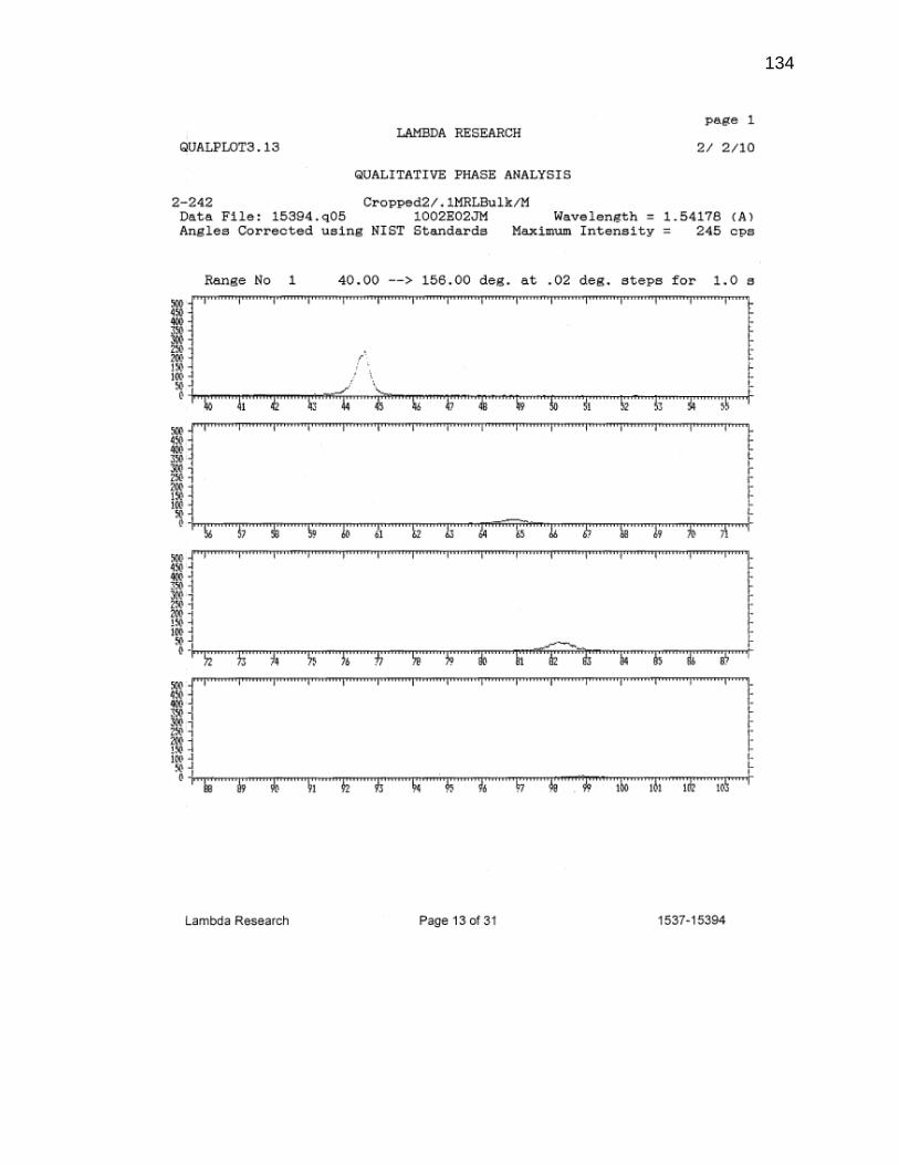
134

135

136

137

138

139

140

141

142
Appendix C
Qualitative Phase Analysis for Carbide Extraction from Lambda Research

143

144

145

146

147

148

149

150

151
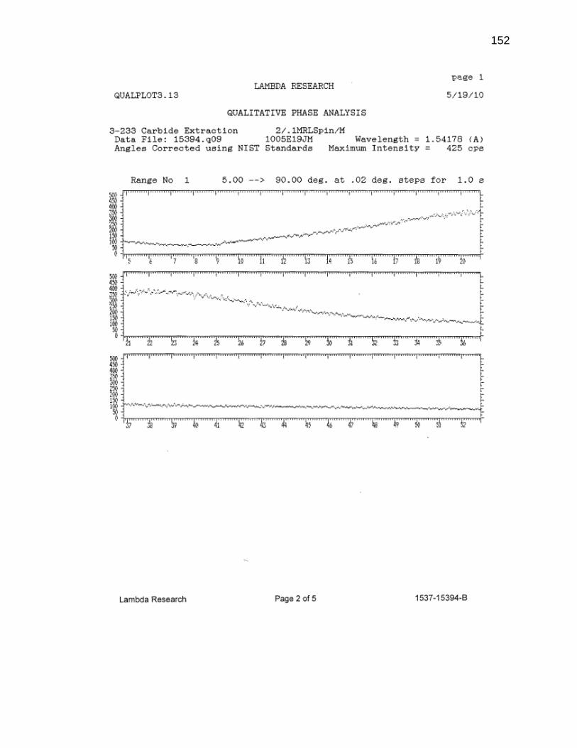
152

153

154

155