THE ECONOMIC FEASIBILITY OF BIOENERGY PRODUCTION FROM

MISCANTHUS FOR THE ONTARIO GREENHOUSE INDUSTRY

A Thesis

Presented to

The Faculty of Graduate Studies

of

The University of Guelph

by

TASNEEM VIRANI

In partial fulfillment of requirements

for the degree of

Master of Science

May, 2011

© Tasneem Virani, 2011

ABSTRACT

THE ECONOMIC FEASIBILITY OF BIOENERGY PRODUCTION FROM

MISCANTHUS FOR THE ONTARIO GREENHOUSE INDUSTRY

Tasneem Virani

University of Guelph

Advisors:

Dr. Richard Vyn and Dr. Bill Deen

This thesis investigates the cost of producing miscanthus in Ontario as an energy crop for

the Ontario greenhouse industry. To determine the breakeven price of growing

miscanthus an enterprise budget was developed and applied to three different life cycle

scenarios to determine the effect of stand life on the breakeven price. The base case

breakeven price of producing miscanthus ranged from $74.74/t to $80.22/t. Sensitivity

analysis was conducted to assess the effect of assumptions (stand yield, rhizome cost,

harvest method and discount rate) on the breakeven price. Price of energy from

miscanthus ranged from $2.87/GJ to $8.63/GJ with an average price of $5.51/GJ. The

Ontario greenhouse industry`s willingness to pay for bioenergy from miscanthus is based

on the prices of fuels currently in use. Ontario farmer‘s willingness to produce

miscanthus is based on its profitability compared to other crops and the time it takes to

pay off the initial investment.

i

ACKNOWLEDGEMENTS

I would like to thank my committee member Dr. Alfons Weersink for his

comments and constructive criticism. A special thanks to my advisors, Dr Richard Vyn

and Dr. Bill Deen for helping me through the completion of this thesis project. Also I

would like to thank the Department of Food, Agriculture and Resource Economics,

faculty, staff and graduate students who made my graduate experience memorable.

I would like to thank my family for their support and for keeping me motivated. A

special thanks to Shiraz for being my sounding board for the last two years. Also I would

like to thank my friends Ken Poon and Sarah Lewis for their contributions.

ii

TABLE OF CONTENTS

CHAPTER 1 INTRODUCTION

BACKGROUND .............................................................................................................................. 1

Sector, size and location ......................................................................................................... 1

Ontario‘s role nationally and internationally .......................................................................... 2

Issues ....................................................................................................................................... 3

Characteristics of an ideal energy crop ................................................................................... 8

Limitations of herbaceous C4 perennials .............................................................................. 12

ECONOMIC PROBLEM ................................................................................................................. 14

RESEARCH PROBLEM ................................................................................................................. 15

PURPOSE .................................................................................................................................... 17

OBJECTIVES ............................................................................................................................... 17

CHAPTER OUTLINE..................................................................................................................... 17

CHAPTER 2 LITERATURE REVIEW ON MISCANTHUS AS AN ENERGY

CROP

ORIGIN ....................................................................................................................................... 19

GENETIC BACKGROUND AND AVAILABILITY OF VARIETIES ........................................................ 20

MANAGEMENT OF MISCANTHUS AS A CROP ................................................................................ 20

Propagation ........................................................................................................................... 21

Input requirements ................................................................................................................ 23

Harvesting ............................................................................................................................. 24

BIOMASS YIELD .......................................................................................................................... 25

COMBUSTION CHARACTERISTICS ............................................................................................... 26

COST OF PRODUCTION ................................................................................................................ 29

CHAPTER SUMMARY .................................................................................................................. 31

CHAPTER 3 DEVELOPMENT IF A MISCANTHUS ENTERPRISE BUDGET AT

THE FARM LEVEL

OVERVIEW OF CONCEPTUAL FRAMEWORK ................................................................................. 34

Demand/Consumption .......................................................................................................... 35

Supply/Production ................................................................................................................. 37

THE MODEL: ENTERPRISE BUDGET ............................................................................................ 39

Duration of stand productivity .............................................................................................. 40

Scenario 1 – Standard scenario ......................................................................................... 41

Scenario 2 – Delayed peak yield establishment scenario ................................................. 42

Scenario 3 – Early termination scenario ........................................................................... 43

Yield ...................................................................................................................................... 45

Input costs ............................................................................................................................. 47

iii

Establishment cost ............................................................................................................ 50

Fertilizer requirements ...................................................................................................... 52

Weed Control .................................................................................................................... 53

Harvesting ......................................................................................................................... 54

Storage .............................................................................................................................. 55

Net present value ................................................................................................................56

Opportunity cost .................................................................................................................... 59

Comparison to other studies ............................................................................................... ...60

SENSITIVITY ANALYSIS .............................................................................................................. 65

Yield of a miscanthus stand .................................................................................................. 65

Rhizome cost ......................................................................................................................... 67

Harvest method ..................................................................................................................... 68

Discount rate ......................................................................................................................... 68

CHAPTER SUMMARY .................................................................................................................. 69

CHAPTER 4 RESULTS AND DISCUSSION

RESULTS .................................................................................................................................... 71

Base case results ................................................................................................................... 72

Yield sensitivity results ......................................................................................................... 73

Rhizome cost sensitivity results ............................................................................................ 75

Harvest method sensitivity results ........................................................................................ 76

Discount rate sensitivity results ............................................................................................ 77

DISCUSSION ............................................................................................................................... 78

Ontario greenhouse industry‘s willingness to pay ................................................................ 81

Optimistic, realistic and pessimistic scenario for miscanthus production.............................88

Ontario farmer‘s willingness to produce ............................................................................... 90

CHAPTER SUMMARY .................................................................................................................. 95

CHAPTER 5 CONCLUSIONS

SUMMARY .................................................................................................................................. 97

PRINCIPLE FINDINGS ................................................................................................................... 98

IMPLICATIONS .......................................................................................................................... 101

SUGGESTIONS FOR FUTURE RESEARCH ..................................................................................... 101

REFERENCES...............................................................................................................103

APPENDIX

APPENDIX A – ENTERPRISE BUDGET FOR STANDARD SCENARIO .............................................. 114

APPENDIX B – ENTERPRISE BUDGET FOR DELAYED PEAK YIELD ESTABLISHMENT

SCENARIO ................................................................................................................................. 117

APPENDIX C – ENTERPRISE BUDGET FOR EARLY ESTABLISHMENT SCENARIO ........................... 120

iv

List of Tables

Table 1.1 Cost per gigajoule of energy produced from coal and natural gas......................5

Table 2.1 Mineral and carbohydrate content for miscanthus samples harvested at two

dates in the Netherlands.....................................................................................................24

Table 2.2 Quality characteristics of biomass, their effects on a boiler system and their

critical limits .....................................................................................................................27

Table 2.3 Comparison of assumptions and cost of production estimates for

miscanthus..........................................................................................................................32

Table 3.1 Review of miscanthus yields from other studies...............................................48

Table 3.2 Fertilizer application rated post-establishment of miscanthus rhizomes...........53

Table 3.3 Return per hectare for corn, soybean and wheat for Ontario in 2009................61

Table 3.4 Cost of production budget for miscanthus, base case for scenario 1.................62

Table 3.5 Cost of production estimate comparison ($/ha).................................................64

Table 4.1 Breakeven price for the base case of all three scenarios....................................72

Table 4.2 Change in breakeven price when harvest method is changed from mow and

bale to using a forage harvester.........................................................................................77

Table 4.3 Sensitivity of breakeven prices…………………..............................................80

Table 4.4 Comparison of assumptions and cost of production estimates for

miscanthus..........................................................................................................................81

Table 4.5 Cost per gigajoule of energy produced by miscanthus as yield of the stand

changes for the base case scenarios...................................................................................83

Table 4.6 Cost per gigajoule of energy produced by miscanthus as discount rate changes

for the three scenarios........................................................................................................83

Table 4.7 Cost per gigajoule of energy produced by miscanthus as the cost per rhizome

changes for all three scenarios...........................................................................................84

Table 4.8 Cost per gigajoule of energy produced by miscanthus as yield changes for

stands harvested using a self propelled harvester..............................................................85

v

Table 4.9 Cost per gigajoule of energy produced from miscanthus, coal and natural

gas......................................................................................................................................87

Table 4.10 Optimistic, realistic and pessimistic scenarios of growing miscanthus in

Ontario...............................................................................................................................90

Table 4.11 Payback periods for the initial investment made to grow a stand of

miscanthus. Revenue is calculated at a rate of $142.35/tonne of miscanthus...................92

Table 4.12 Expected net revenue of various Ontario crops..............................................93

Table 4.13 Expected net revenue for the three base case scenarios of miscanthus...........94

vi

List of Figures

Figure 1.1 Greenhouse area in the various provinces of Canada from 1999 to 2007

(ha).......................................................................................................................................4

Figure 1.2 Price of natural gas and coal in Canada from 2002 to 2009 ($/GJ)....................6

Figure 3.1 Conceptual framework graph depicting the breakeven point, economic loss

and economic profit of a farm level miscanthus enterprise...............................................36

Figure 3.2 Lifecycle scenarios for a stand of miscanthus..................................................44

Figure 4.1 Change in breakeven price as yield of a miscanthus stand changes.................74

Figure 4.2 Change in breakeven price as the cost per rhizome changes............................76

Figure 4.3 Change in breakeven price as the discount rate increases................................78

1

Chapter 1: Introduction

1.1 Background

The greenhouse industry is one of the fastest growing agricultural sectors in Ontario and

has experienced constant growth since the late part of the 20th century (Planscape 2009).

Studies show that the greenhouse industry ranks as one of the highest in gross farm

receipts generated, despite the minimal area farmed. For example, in 2006 the Ontario

greenhouse industry represented 11% of gross farm gate receipts in Ontario (Planscape,

2009). Greenhouse production is heavily intensive in its use of land, and therefore,

generates much higher returns ($43,492/ ha in 2006) than field agriculture ($245/ha, an

average from 2005 to 2009) (Planscape, 2009, OMAFRA, 2010).

1.1.1 Sectors, size and location

The greenhouse industry is divided into two major sectors - the Ontario

greenhouse vegetable growers (OGVG) and the greenhouse floriculture sector. Between

2001 and 2006 the largest percentage increase in area took place in vegetable production.

While floriculture leads in number of operations, characterized by many small farms and

a few large producers, vegetable production dominates in terms of area covered (Brown

et al., 2010, Planscape, 2009). The average greenhouse operation (for floriculture and

vegetable sector) in Ontario is just over 3,600 square meters according to the 2006

Agricultural census (Brown et al., 2010). On the whole, between 2001 and 2006, the

number of greenhouse operations declined by 6%, while the area under cover increased

by 29% and the value of production increased by 23%. These figures confirm an ongoing

2

trend in the greenhouse sector of fewer operations but a higher area under cover

(Planscape, 2006; Brown et al., 2010).

The largest conglomeration of greenhouses in Ontario (75%) is situated in

southern Ontario in the counties/regions located around the western end of Lake Ontario,

such as Niagara and Hamilton, and the counties along the north shore of Lake Erie, in

particular Essex, Haldimand and Norfolk (Brown et al., 2010). Of all the counties, Essex

County has the largest group of greenhouses (209 operations), and the largest area under

cover. Ninety percent of greenhouses in Essex County are dedicated to vegetable

production, up from 87% in 2001. Eighty- two percent of the greenhouses in Niagara are

dedicated to flowers, a decrease from 84% in 2001 (Planscape, 2009). Kingsville, the

municipality next to Leamington has the second largest cluster. In the region of Niagara

in 2006, the largest clusters of greenhouses were found in the Town of Lincoln, St.

Catharines and Niagara-on-the-Lake respectively (Planscape, 2009).

1.1.2 Ontario’s role nationally and internationally

The greenhouse sector makes a significant contribution to the provincial

economy. In 2006, gross farm receipts of $1.15 billion were generated by the Ontario

greenhouse industry. In 2007, Ontario accounted for over 50% of the total Canadian

floriculture sales and 56% of total greenhouse vegetable sales (Planscape, 2009). Among

North American jurisdiction, Ontario is the third largest producer of greenhouse

floricultural products (generating $742 million dollars) behind California ($1.02 billion

U.S.) and Florida ($922 million U.S.) (Brown et al.,2010).

3

Sales of the Ontario greenhouse vegetable and floriculture sectors reached the 1

billion dollar mark in 2001. Analysis of this economic activity in 2006 confirmed that

that based on $1.1 billion in sales, the greenhouse sector would generate $3.9 billion in

annual economic activity in the province (Planscape, 2006). The sale level increased to

$1.7 billion in 2004 fell back to $1.2 billion in 2005 and rose to $1.15 billion in 2006. In

2007, sales were reported at $1.2 billion. Consistently, sales have exceeded $1.1 billion

and therefore would have continued to have an annual economic impact of $3.9 billion or

more on the provincial economy (Planscape, 2009).

After experiencing 18 years of continuous growth, the Canadian greenhouse area

expansion ended in 2007. Between 2006 and 2007, Statistics Canada reported a decrease

nationally of approximately 164,000 sq metres of area under cover. Ontario did not

contribute to the decline, rather area under cover in Ontario increased between 2006 and

2007. The share of Canada‘s total greenhouse production acreage located in Ontario rose

from 51% in 2004 to 55% in 2007 (Planscape, 2009).

Ontario continues to lead the country in greenhouse production and that

dominance increased proportionately from 2006 – 2007. While the area in greenhouse

production in Canada as a whole remained relatively static, the area in Ontario increased.

Figure 1.1 shows the greenhouse area in Ontario relative to other provinces.

1.1.5 Issues

Although the greenhouse industry in Ontario is growing and vibrant, there are a number

of challenges the industry faces. Operating costs for greenhouses are high with the most

4

significant costs being for labour and fuel (Brown et al., 2010). Labour costs tend to

increase proportionately as area under production increases. This type of cost is easier to

address and forecast. Conversely, fuel costs are subject to market pressures and can

fluctuate significantly

Figure 1.1: Greenhouse area in various provinces of Canada from 1999 to 2007 (ha) (Statistics Canada - Greenhouse, Sod and Nursery Industries - Catalogue No. 22-202-XIB, 2000

to 2007)

from season to season (Planscape, 2006). A study done by Brown et al. (2010) estimated

heating costs to be equal to 20% to 35% of the total operating costs, depending on the

crop being grown. The months of December to February represent 58% of the total

annual heating requirements. Calculations based on data from Statistics Canada (table 4

of Catalogue 22-202-XIB, 2007) suggested that 40% of annual operating expenses

incurred by an Ontario greenhouse were heating costs. This was an average annual value

0

200

400

600

800

1000

1200

1999 2000 2001 2002 2003 2004 2005 2006 2007

Are

a (

hec

tare

s)

Year

Ontario

Quebec

British Columbia

All Other Provinces

5

calculated for 1,500 greenhouses in Ontario. The actual heating cost varied (fluctuated

between 20% and 58%) by time of year and location of the greenhouse.

Most greenhouses are heated with the use of coal, oil or natural gas or a

combination of the three (personal communication, Shalin Khosla, March 30, 2010).

Natural gas and coal are the two primary fuels that are used. Oil is usually used as a

backup system for times when extra energy is required to heat the greenhouse facilities.

Of the two primary fuels, natural gas is easier to use. Greenhouses that use natural gas

for heat get the fuel delivered to their facilities using pipelines; therefore relieving owners

of the responsibility to store or handle the fuel (personal communication, Shalin Khosla,

March 30, 2010). While the natural gas system is easy to operate it is more expensive.

Table 1.1 compares the cost per gigajoule of energy produced from coal and natural gas.

The price of coal is determined by averaging the prices published in the Canadian mineral

year book from 2002 to 2009. The Canadian mineral year book is a publication of the

Ministry of Natural Resources. The price of natural gas includes the cost of delivery and

is determined by taking a five year average (January 2006 to July 2010) from the Ontario

Energy board.

Table 1.1: Cost per gigajoule of energy produced from coal and natural gas (2002 –

2009).

Fuel Coal Natural Gas

Cost range ($/GJ) $1.99/GJ - $9.49/GJ $3.83/GJ -$8.14 /GJ

Average Cost ($/GJ) $4.50/GJ $6.20/GJ

Source: Price of coal was calculated from the Canadian Mineral Year Book (2002 –

2009). Natural gas price was calculated from Natural Resource Canada (2002 – 2009)

6

From table 1.1 it can be observed that coal is less expensive than natural gas.

However, like natural gas and oil, coal is a non-renewable fuel and prone to price

fluctuations depending on global market conditions (personal communication, Shalin

Khosla, March 30, 2010). Figure 1.2 depicts the price fluctuations of natural gas and coal

from 2002 to 2009. The price of natural gas in 2002 was $3.83/GJ and increased to a peak

high of $8.14/GJ in 2005. Even though there seems to be a downward price trend since

2005, the fluctuations have continued. Similar to natural gas, the price of coal seems to be

erratic and has an upward trend.

Figure 1.2: Price of Natural Gas and Coal in Canada from 2002 to 2009 ($/GJ)

Source: Price of Natural gas was taken from Natural Resource Canada. Price of coal was

taken from the Canadian Mineral Year Book.

The Ag Energy Co-Operative, an industry owned company, has tried to cushion

some of the fuel cost increases through volume purchases and long term contracts.

However in the past five years (2005 to 2009), fuel costs have increased by 30% while

0.00

1.00

2.00

3.00

4.00

5.00

6.00

7.00

8.00

9.00

10.00

2002 2003 2004 2005 2006 2007 2008 2009

Pri

ce (

$/G

J)

Year

Coal

Natural Gas

7

wholesale prices of greenhouse products have increased by less than 3% (Brown et al.,

2010).

Both coal and natural gas are fossil fuels and contribute to the increasing carbon

dioxide content in the atmosphere (Lewandowski et al., 1996; Clifton-Brown et al.,

2007). The carbon dioxide content of the atmosphere is projected to increase by almost

50% over the first 50 years of this century. The major cause of this increase is continued

combustion of fossil fuels (Heaton et al., 2003). The environmental degradation caused

by fossil fuels and the increase in energy costs has encouraged greenhouse owners to look

for alternate sources of energy. Around 20% of greenhouse owners have switched to

using biomass (personal communication, Shalin Khosla, March 30, 2010). Biomass is a

renewable source of energy that is carbon neutral. Although carbon dioxide is released by

combusting biomass, the quantity does not exceed the amount that was fixed previously

by photosynthesis while the plants were growing (Lewandowski et al., 1997). Complete

carbon neutrality cannot be achieved even with biomass because the carbon that is

released by the planting and harvesting machinery of the crop is in excess to carbon that

is released during combustion. However, the overall carbon released by biomass

combustion is much less than that of fossil fuels (Atkinson, 2009). Biomass can either be

used directly for combustion or after having been converted into oil, ethanol or gas. It is

important to know the energy efficiency of a crop when it is being used as a source of

biomass. Energy efficiency of a crop is determined by dividing the energy output from

the crop by the amount of energy required in production. A crop with high energy

efficiency would provide higher energy output and have lower energy requirements

during production, compared to a low energy efficiency crop (Lewandowski et al., 1997).

8

The ratio of energy output to energy input in the production of Miscanthus is 14.5 – 19.7

and thus much better than that of whole grain crops with a ratio of 8.5 (Lewandowski et

al., 1995). In the production of ethanol the ratio lies between 1.3 for sugar beets and 5.0

for sugar sorghum, depending on the extent to which by-products are used. For the

production of partly refined rape-oil it is about 5.7. Thus, according to Lewandowski et

al. (1997), the direct combustion of biomass is the most energy efficient alternative with

the highest potential for preventing CO2 emissions.

Biomass can be combusted for a greenhouse using the same boiler system that is

used for burning coal, so any grower using coal can switch to biomass without incurring

any additional capital cost. Wood chips, soybean, corn and other agricultural wastes are

examples of some of the biomass sources that have been used so far by the greenhouse

industry (personal communication, Shalin Khosla, March 30, 2010). However, none of

these sources have been able to successfully fulfill the energy requirements. Section 1.2

outlines some of the characteristics that are required in a crop for it to be an ideal energy

source.

1.2 Characteristics of an ideal energy crop

An ideal biomass crop is characterized by attributes that allow it to capture and

convert solar energy into harvestable biomass with maximum efficiency using minimum

inputs and having minimal environmental impacts. A biomass crop requires low

investments of energy (fossil fuels) and money if it is to be environmentally and

commercially viable, while still providing clean, cost-effective fuel (Lewandowski et al.,

9

2003). According to Heaton et al. (2003), the ideal crop would have the following

properties:

a. Energy balance: The crop should have a favourable energy balance, where there is

low energy input and high energy output. Perennials have a lower input to output

ratio (<0.2) compared to annuals (>0.8).

b. Maximum efficiency of light use: A good fuel crop should maximize biomass

development per unit area and per unit investment. Biomass development would

be dependent on the amount of light available. Crops that maintain a closed

canopy would have greater biomass and would also cut off sunlight from the

weeds, reducing number of weeds and herbicide use.

c. Water content and water use efficiency: Energy crops should have low water

content and use water efficiently. Low water content will make combustion of the

crop easier, and decrease the input of energy for drying the biomass. Additionally,

if the crop uses water efficiently than the cost of irrigation would go down.

d. Nitrogen (N) and nutrient use efficiency: In addition to water and light efficiency

the crops need to be efficient with N and nutrient use. This property will help to

minimize both the quantities of N that need to be applied as fertilizer and the

amount lost to drainage water (Long 1994). Perennial rhizomatous grasses (PRG)

are known to relocate the nutrients from their leaves and stems into their

underground rhizomes, at the end of the vegetation period, thereby increasing

their nutrient use efficiency. This also improves the biomass quality for

combustion (Lewandowski et al., 1997)

10

e. C4 photosynthesis: C4 photosynthesis is a method of carbon fixation in which

carbon dioxide from the air is incorporated into a 4-carbon compound during

photosynthesis. Plants that undertake C4 photosynthesis are estimated to have

40% greater biomass energy than C3 plants (Beale, 1999). C4 photosynthesis also

allows for plants to have higher efficiencies of nitrogen and water use (Ehleringer

et al., 1997).

f. Minimizing changes in land use and farm machinery: Energy crops will have

greatest acceptability and minimal costs of conversion, if the plants selected as

fuel crops can i) be planted and harvested with the machinery used for food

crops; ii) be easily eradicated should the landowner subsequently want to change

land use, and iii) provide harvestable material in a short period of time (Beale et

al., 1999).

g. Environmental impacts and benefits: Often highly productive species are invasive

and out-compete the native species. Hence it is environmentally advantageous if

the fuel crop grown is sterile.

All the above characteristics can be found in perennial rhizomatous grasses (PRGs).

PRGs, especially those using the C4 photosynthetic pathway, typically use nutrients,

water, and solar radiation more efficiently than other plants (Christian et al., 1997). The

perennial rhizome system allows nutrients to be cycled seasonally between the above and

below ground portions of the plant, thus minimizing external additions of fertilizer

(Lewandowski et al., 2000). Furthermore, since they have few natural pests, they may

also be produced with little or no pesticides (Lewandowski et al., 2003). If the crop is

harvested after the leaves have dropped in winter, and associated nutrient translocation

11

(movement of nutrients from the shoots and leaves to the roots) has occurred, the

resultant fuel will have a lower mineral content and therefore release little pollution when

combusted (Lewandowski et al., 1997). Such physiological aspects allow PRGs to

provide clean fuel and more dry matter per unit of input compared to other potential

biomass crop options (Heaton et al., 2003).

There are also many ecological benefits expected from the production and use of

perennial grasses. The substitution of fossil fuels by biomass is an important contribution

in reducing anthropogenic CO2 emissions. Compared to other biomass sources, like

woody crops and other C3 crops, C4 grasses may be able to provide more than twice the

annual biomass yield in warm and temperate regions because of their more efficient

photosynthetic pathway (Heaton et al., 2004). Unlike annual crops, the need for soil

tillage in perennial grasses is limited to the year in which the crops are established,

reducing cost and fossil fuel use. Perennials also have more extensive root systems than

annuals, which are present throughout the year. The long periods without tilling and an

extensive root system reduce the risk of soil erosion and a likely increase in soil carbon

content (Hallam et al., 2001). Additionally, studies of fauna show that due to long-term

lack of soil disturbance, the late harvest of the grasses in winter to early spring and

insecticide-free production causes an increase in abundance and activity of different

species, especially birds, mammals and insects, in the stands of perennial grasses

(Lewandowski et al., 2003). Perennial grasses can therefore contribute to ecological

values in agricultural production.

12

1.3 Limitations of Herbaceous C4 Perennials

Though in theory C4 perennial rhizomatous grasses come closest to the specified

ideal fuel crop, they have disadvantages in practice when cultivated in cool temperate

climates of the continental U.S., southern Canada, and northern Europe. While there are a

wide range of C4 herbaceous perennials, the vast majority are tropical in origin, and show

a high temperature threshold for leaf growth and a susceptibility to low temperature

dependent photoinhibition of photosynthesis (Ehleringer et al., 1997). Miscanthus

however, appears exceptional. It develops its canopy early, even at 52 degrees north, and

forms photosynthetically competent leaves at 10 degrees Celsius. At 52 degrees north it

can yield over 20 t/ha of biomass, yet show the high N-use and water-use efficiency

characteristic of C4 plants at warmer temperatures (Beale et al., 1997).

Miscanthus has been studied extensively in Europe (Lewandowski et al., 2000;

Styles et al., 2008) and the U.S. (Heaton et al., 2003; Khanna et al., 2008), but to date no

reports of miscanthus studied as a biofuel in Canada have been published in the peer

reviewed literature. Feasibility of miscanthus as an alternative energy source is dependent

on many factors including yield potential, input requirements, combustion properties, and

heating system conversion costs. Research in Europe, and more recently in Illinois, has

confirmed the potential for high biomass production from miscanthus. For example,

results from field trials in Illinois found that miscanthus produced more than double the

per-acre biomass of switchgrass (Khanna et al., 2008). Similar to other biomass sources,

miscanthus is a renewable fuel, burns cleaner than coal and is subject to relatively small

price fluctuation. In addition, its potential for high yield can make miscanthus a very

13

profitable crop to produce, and it may be a very economical source of energy for the

Ontario greenhouse industry.

While studies on miscanthus have been conducted in other countries, it is

important to study miscanthus in a Canadian context to account for the environmental

differences. Cold temperatures and high levels of precipitation during the winter can

delay establishment of the stand, reduce yield and negatively affect the biomass quality.

Since the quantity and quality of biomass has an economical impact, accounting for these

changes is an important part of this study. While this study uses an enterprise budget

similar to the one used by Khanna et al, 2008 it applies Canadian prices for inputs and

uses yield estimates that account for the Canadian environmental differences. Currently,

miscanthus is being evaluated in field trials in Ontario for yield potential and combustion

properties. This research is funded through the Ontario Ministry of Agriculture, Food and

Rural Affairs (OMAFRA) Alternative Renewable Fuels research and development

program. However, this research does not specifically examine the economics of the use

of miscanthus as an alternative energy source.

To address this gap in the research, an economic feasibility study is required to

determine whether miscanthus would be an economic source of biomass energy for the

greenhouse industry. The influence of factors such as yield variation, input costs, and

storage costs on the economic feasibility will also be considered as part of this study.

14

1.4 Economic Problem

The increasing price of energy from fossil fuels has had an adverse effect on the

profitability of the greenhouse industry, and as a result the industry is looking for cheaper

sustainable alternatives. The ability of miscanthus to produce high yields for biomass

combustion could make it a good source of sustainable energy for the greenhouse

industry. Although miscanthus has been extensively studied in Europe and the U.S. as a

source of biomass, the cost of growing miscanthus in Ontario is unknown.

If miscanthus is to be adopted as an energy source by the greenhouse industry in

Ontario it is important to know the cost of producing miscanthus and the Ontario

greenhouse industry‘s willingness to pay for it. Miscanthus can be economically viable

option for the Ontario greenhouse industry only if its cost per gigajoule is less than that of

fossil fuels currently in use. To determine the economic viability of miscanthus the

following questions need to be addressed:

1. How does the life cycle of a miscanthus stand affect the cost of

production?

2. What is the yield per hectare of miscanthus given the soils and weather in

Ontario and how does yield affect the cost of production?

3. What are the costs of inputs in Ontario?

4. What are the prices of other energy sources and how does that affect the

Ontario greenhouse industry‘s willingness to pay for miscanthus?

15

An economic feasibility study comparing the cost of energy production from

miscanthus with other fossil fuels will help the Ontario greenhouse industry decide if

miscanthus is a cheaper option than fossil fuels to heat their facilities. Furthermore, since

Ontario farmers will be growing this crop it is important to determine their willingness to

grow miscanthus.

1.5 Research Problem

The research problem is to develop an economic feasibility study for growing

miscanthus in Ontario as a source of biomass for the Ontario greenhouse industry, using

input costs from Ontario.

This study builds on the biological and economic research already done in

Europe and the U.S. Since previously conducted studies are site specific, their results

vary considerably. For example, Styles et al. (2008) conducted a life cycle cost

assessment for a 14- cut miscanthus plantation in Ireland. The assessment was based on a

farm operation sequence for multiple supply and harvest strategies. The cost of each

activity was taken from the literature and converted to 2009 prices. The competitiveness

of miscanthus in relation to other energy sources was compared using the net present

value method. Venturi et al. (1998) compared the cost of different production chains of

miscanthus in Europe, with a focus on the equipment used in the harvesting and

transportation of miscanthus. Yield and input estimates were based on the values

available in the literature. The study assessed three transport systems and eight harvest

machines and calculated the fixed and variable costs of all the equipment used. The study

also calculated the change in costs if part of the production process was carried out by a

16

contractor rather than the farmers themselves. Finally, Khanna et al. (2008) developed a

twenty year enterprise budget for miscanthus to determine the farm gate breakeven price

of the energy crop. Yield was determined using a biophysical model and land costs were

not included. The cost of transportation was later added to the breakeven price. Unlike

the other two studies, the yield and input estimates of this study were based on

environmental conditions in the U.S. and only one production chain was considered.

Since the method used by Venturi et al. (1998) focuses on the cost of the

machinery used in the production of miscanthus, it would not adequately answer the

questions posed in the previous section. A combination of the methods used by Khanna et

al. (2008) and Styles et al. (2008) can help determine the cost of producing miscanthus in

Ontario. An enterprise budget, similar to the one developed by Khanna et al. (2008), with

Ontario input prices would determine the farm gate breakeven price of growing

miscanthus in Ontario. Different harvest and storage methods can be assessed using the

enterprise budget to compare the possible production chains available to farmers. Finally,

the net present value method used by Styles et al. (2008) can be employed to compare the

cost of producing energy from miscanthus with other fossil fuels. All input prices and

estimates would need to be Ontario specific to answer the questions of the Ontario

greenhouse industry.

To determine the Ontario farmer‘s willingness to grow miscanthus, the profit

from miscanthus could be compared to the profit made from other crops. If the profit

generated from miscanthus is equal to or more than the profit farmers receive from

17

growing other crops, farmers may be willing to grow miscanthus in Ontario for the

greenhouse industry.

1.6 Purpose

The purpose of this research is to assess the economic viability of miscanthus as a

source of heat energy for the Ontario greenhouse industry, relative to the current sources

such as coal and natural gas.

1.7 Objectives

This research project will achieve four objectives related to the economic

efficiency of miscanthus. The objectives of this study are to:

1. Determine the cost of miscanthus production and the breakeven value in Ontario

by developing a farm level enterprise budget with input cost values from Ontario.

2. Conduct a sensitivity analysis on the cost of production to determine the effect of

various assumptions on the breakeven value of miscanthus production.

3. Estimate the Ontario greenhouse industry‘s willingness to pay for bioenergy from

miscanthus by determining the price the industry pays for its current fuel sources.

4. Determine Ontario farmer‘s willingness to produce miscanthus by comparing the

profits of their current crops to the profits from miscanthus.

1.8 Chapter Outline

To provide some background on miscanthus, chapter 2 will cover the origins and

genetic background of miscanthus, management methods and requirements as well as

18

combustion characteristics of the crop. This chapter will also review some of the cost

estimates made by other studies on growing miscanthus.

Chapter 3 will develop the conceptual framework of the study and outline some of

the assumptions with respect to the life cycle of a miscanthus stand. It will then develop a

farm level enterprise budget for growing miscanthus in Ontario and explain the need for a

sensitivity analysis.

Chapter 4 will present the results of the base enterprise budget as well as the

results of the sensitivity analysis. The costs per gigajoule of producing energy from

miscanthus will then be compared to the cost per gigajoule of energy from other fuel

sources to determine if using miscanthus as a source of bioenergy is an economically

feasible option for the Ontario greenhouse industry. Profits from growing miscanthus as a

crop will be compared to profits from other crops commercially grown in Ontario to

determine the farmer‘s willingness to produce miscanthus.

Chapter 5 summarizes the methods used in the study and highlights the principal

findings of the study. Suggestions for future research are also provided.

19

Chapter 2: Literature review on miscanthus as an energy crop

In order to understand the advantages of using miscanthus as an energy crop, this

chapter provides a background on miscanthus based on experiences from the European

Union as well as the U.S. The background on miscanthus includes its origin; genetic

background and availability of varieties; management requirements including

propagation techniques, input requirements and harvesting techniques; as well as the

biomass yield recorded in various countries. Finally the chapter examines the economics

of growing miscanthus by presenting the cost estimates made by other studies done in the

European Union and the U.S.

2.3 Origin

Miscanthus consists of 17 species and can be divided into four sections —

―Kariyasua‖, ―Diandra‖, ―Thiarrhena‖ and ―Eumiscanthus‖. The genetic origin of

miscanthus is in East-Asia, where it is found throughout a wide climatic range from

tropical to subtropical., and warm temperate parts of Southeast Asia to the Pacific Islands

(Lewandowski et al., 2003). There can be frequent naturally occurring hybridization

within the genus. The genotype widely used in Europe for productivity trials and

commercial purposes, miscanthus × giganteus (M. giganteus), was introduced from Japan

to Denmark in 1930 (Lewandowski et al., 2003). M. giganteus is believed to have

miscanthus sinensis (M. sinensis) and miscanthus sacchariflorus (M. sacchariflorus) as its

parents (Farrell et al., 2006). Cultivars of M. sinensis have been widely planted in the

United States and Europe as landscape ornamentals (Huisman et al., 1997).

20

2.4 Genetic background and availability of varieties

Of the four sections of miscanthus only the latter two sections (―Thiarrhena‖ and

―Eumiscanthus‖) contain genotypes of interest for biomass production (Lewandowski et

al., 2003). The basic chromosome number of miscanthus is 19. The triploid genotype M.

giganteus has 57 somatic chromosomes, and is probably a natural hybrid involving M.

sacchariflorus (diploid, section Eumiscanthus) and M. sinensis (tetraploid, section

Thiarrhena) (Lewandowski et al., 2003). As a consequence of its triploidy, M. giganteus

is sterile and cannot form fertile seeds (Lewandowski, 2003). The two species of

miscanthus that are of interest for breeding genotypes for bioenergy are M. sacchariflorus

and M. sinensis. M. sacchariflorus genotypes are more adapted to warmer climates,

whereas M. sinensis genotypes are more winter hardy (Lewandowski, 2003). The aim of

miscanthus breeding for bioenergy is the production of hybrids that in some aspects are

similar to M. giganteus. Desirable characteristics include a high biomass yield potential

and sterile seeds. Seed sterility of hybrids is preferred to prevent seed escape from

miscanthus stands (Khanna et al., 2008; Lewandowski et al., 2008).

2.5 Management of miscanthus as a crop

This section outlines the requirements for growing miscanthus on a farm. It begins

by reviewing the various methods of propagation currently available, the input

requirements of the plant and the harvesting methods to be used.

21

2.5.1 Propagation

The majority of the studies in the literature focus on the genotype M. giganteus - a

sterile hybrid - that needs to be propagated vegetatively using either rhizomes or tissue

culture. However, a study done by Atkinson (2009) outlines four types of miscanthus

propagation systems

a. Seed production system: This production system would only work for the

miscanthus species that flower and are not sterile. Miscanthus species generally

do not flower either due to environmental limitations or because certain hybrids

are sterile. While the self-sterile habit of M. giganteus prevents its establishment

from seed that is not the case with M. sinensis which flowers in the UK, albeit of

variable seed viability (Christian et al., 2005). Miscanthus seeds are very small

(1000 seeds weigh about 250–1000 mg), have low nutrient reserves, and require

high temperature and moisture for germination (Lewandowski et al., 2003). Crop

establishment with M. sinensis from seed is possible if drilled with pelleted seed.

Work with M. sinensis clones suggested to be superior to M. giganteus are being

developed with more economic seed propagation methods (Atkinson, 2009).

b. In vitro propagation system: In vitro cultivation with the use of plantlets is known

as micro-propagation. Two basic micro-propagation techniques are available.

Direct regeneration of shoots can be achieved by using axillary nodes or apical

meristems. These shoots are then tillered in vitro often using the phytohormone

IAA (indole 3-acetic acid) (Lewandowski, 1997). Another micro-propagation

technique is based on the induction of somatic embryoids from somatic tissue and

22

the regeneration of these embryoids to plants. For promoting the regeneration of

the embryoids to plants, cytokinins such as BAP (benzylaminopurine) are often

used (Lewandowski et al., 1998).

c. Rhizome production system: Propagation with the use of rhizomes is known as

macro-propagation. The method of macro-propagation was first developed in

Denmark. According to this method, nursery fields are subjected to 1to 2 passes

of a rotary tiller after 2-3 years, breaking up rhizomes into 20-100g pieces

(Lewandowski et al., 2000). Rhizome pieces are collected with a stone picker,

potato or flower bulb harvester from nursery fields (Lewandowski et al., 2000).

The rhizomes are then planted in the field using a potato planter (Khanna et al.,

2008). Storage time between the collection and planting of rhizomes needs to be

as short as possible to avoid their drying out. Macro-propagation yields a

multiplication factor of up to 50 times, compared to about 100 times for hand

cutting of rhizomes from the mother plant (Venturi et al., 1998; Lewandowski et

al., 2000).

d. Stem cutting system: Utilizing nodal stem sections as a source of clonal material

is well practiced in agricultural species, such as sugarcane, a close relative of

miscanthus. A similar propagation system may be appropriate for clonal

miscanthus production. (Atkinson, 2009). Producing new plants from stem

cuttings requires that each nodal section has a dormant viable bud capable of

shoot growth and development of associated adventitious roots. Compared to

other methods of propagation, plants propagated via clonal material may be more

23

vulnerable to pathogens and pests due to a lack of genetic diversity in

monocultures (Atkinson, 2009).

2.5.2 Input requirements

A stand of miscanthus has very low input requirements of fertilizers and

herbicides. Based on trials done on several sites in Europe, Lewandowski et al. (2003)

concluded that nitrogen (N) fertilization was necessary mainly on soils with low N

contents. At locations with sufficient N mineralisation from soil organic matter, N

fertilization could be avoided or limited to 50–70 kg per hectare per year. In general,

there is no consensus in the literature on the effect of N fertilization on the yield of the

stand. Phosphorous and potassium were applied at the rate at which the nutrients were

removed from the soil by the plant. The overall nutrient requirements per tonne of dry

matter was estimated to be 2 – 5 kg N, 0.3 – 1.1 kg phosphorus (P), and 0.8 – 1 kg

potassium (K). Similar estimations were made by Pyter et al. (2009) for trials done in the

U.S.

Herbicide requirements are also minimal for a stand of miscanthus. Weed control

is only required in the establishment phase (first 2 – 3 years) since vigorous canopy

growth and ground leaf-litter are assumed to suppress weed growth once the stand is

established (Styles et al., 2008). Various herbicides suitable for use in maize or other

cereals can be used. To date, there are no reports of plant diseases significantly limiting

the productivity of miscanthus (Lewandowski et al., 2003).

24

2.5.3 Harvesting

A stand of miscanthus is expected to be productive for 20 years (Lewandowski et

al., 2000; Khanna et al., 2008). The stand is harvested regularly in the spring of the

following year, except in the first year to ensure good establishment (Khale et al., 2001).

Miscanthus can be harvested only once a year, since multiple cuttings would over-exploit

the rhizomes and kill the stands. The harvest window depends on the local conditions and

is between November and April. The later the harvest can be performed, the more the

combustion quality improves since the moisture content and the mineral content

decreases. Table 2.1 from Lewandowski et al. (2000) shows an example of the decrease

in mineral contents between November and January. Delaying stand harvest by two

months decreases nitrogen (N) content by 23%, potassium (K) content by 21 % and

phosphorous (P) content by 100%. In addition, moisture content has been shown to

decrease from 70% in November to 20% or less by March or April (Lewandowski et al.,

2000).

Table 2.1: Mineral and carbohydrate content in miscanthus samples harvested at

two dates in the Netherlands

Mineral content

(% dry matter)

Harvest date

19th

November 1997 29th

January 1998

N 0.47 0.36

P 0.06 0.00

K 1.22 0.96

Source: Lewandowski et al., 2000

However, there is a trade-off, since the biomass yield decreases as well (Pyter et al.,

2009). According to Lewandowski et al. (2003), delayed harvest can cause a yield loss of

25

up to 25%. For economic reasons, a late harvest at water content lower than 20% is

recommended because the costs for harvesting and drying of the biomass increase with

the water content (Huisman, 1994; Lewandowski et al., 2003).

Available harvesting methods are applicable for harvesting miscanthus (Pyter et

al., 2009). Huisman et al. (1994) suggested that mowing and baling would reduce volume

and make storage easier. Venturi et al. (1997) have suggested that a forage harvester used

for harvesting silage maize or grass can also be used for harvesting miscanthus. The

forage harvester would chop the crops and blow it into a trailer. The number of trailers

involved in transport from the field to the farm would depend on the transport distance

and yield.

2.6 Biomass yield

The 20 year life of a miscanthus stand can be divided into an increasing yield

phase and a plateau yield phase. The first phase is characterized by an increase in

biomass from year to year and constant development of the below-ground storage system

(rhizomes and roots). This phase lasts between 3 to 5 years depending on the site (Khale

et al., 2001). During the plateau yield phase the stand can achieve a peak yield of up to

40 t/ha depending on the climate of the country, soil type, water availability and

miscanthus genotype (Lewandowski et al., 2000). For example, yields above 30 t/ ha are

reported for locations in southern Europe with high annual incident global radiation and

high average temperatures, but only with irrigation. In central and northern Europe (from

Austria to Denmark) where global radiation and average temperatures are lower, yields

without irrigation ranged from 10t/ ha to 25 t/ ha (Lewandowski et al., 2003). Another

26

long-term study done in the UK reported average yields of 13.4 t/ ha (Atkinson, 2009).

Yields from this study declined after 10 years of growth, but other work in the UK, over

12 years of cropping, showed no yield decline (Atkinson, 2009). Trials done in Illinois,

U.S. with M x giganteus had yields between 22 t/ha and 35.5 t/ha (Pyter et al., 2009).

In general miscanthus stands are easier to establish on lighter soils, but in the long

run yields are higher on heavy soils (Lewandowski, 2003). This is explained mainly by

the improved water availability in heavy soils. In temperate and tropical countries, given

the same soil conditions, the yield potential of M. sinensis genotypes is inferior compared

to M. giganteus (Lewandowski, 2003). However, in more northern, cooler regions, such

as Denmark, M. sinensis genotypes from Japan can reach similar yields as M x giganteus

(Jorgensen, 1997). In southern and central Europe M. giganteus is still a very productive

genotype; however, new hybrids are being produced that can match or even out-yield M.

giganteus at central to southern European locations (Clifton-Brown et al., 2001).

2.7 Combustion characteristics

For an energy crop to be compatible for combustion in a boiler system, the biomass from

the crop needs to have low water and mineral content. Mineral content in the biomass is a

result of nutrients that are taken up by the plant from the soil. Table 2.2 from

Lewandowski et al. (1997) outlines the critical limits of the various minerals that may be

found in biomass. During combustion, the mineral components of biomass transform to

form slag and fly ash. The slag softens at the combustion temperature and mineral

deposits start to build up on the interior surfaces of the boiler system (Szemmelveisz et

al., 2009). Significant build up of slag deposits can reduce the efficiency of the boiler

27

system and quickly erode the boiler tubes (Szemmelveisz et al., 2009). Eroding of the

boiler tubes is called corrosion. Corrosion and slagging reduce the durability of the boiler

system and both can be minimized by using biomass with low mineral content.

Table 2.2 Quality characteristics of biomass, there effects on a boiler system and

their critical limits

Quality

Characteristic

Effect Critical limit

Water concentration More emissions, decreasing heating value and

efficiency, decreasing storability.

Less than 230

g/kg

Nitrogen

concentration NOx emissions 10 g/kg DM

Chlorine

concentration Corrosion, HCl emissions, Dioxin emissions 2 g/kg DM

Potassium

concentration Corrosion

Difficult to

quantify

Source: Table taken from Lewandowski et al. 1997

Biomass containing high mineral levels also increases the emission levels of NOX,

SO2, and other gases (Lewandowski et al., 1997). NOx is produced during the

combustion process when nitrogen and oxygen react at elevated temperatures. The two

elements combine to form NO or NO2. Similarly SO2 is formed when oxygen and sulphur

combine at high temperatures in the boiler system. Gases such as NOx and SO2 are a

cause for concern because emission of these gases can result in potential climatic

changes, such as the formation of ground level ozone and acid rain (Szemmelveisz et al.,

2009).

Additionally, moisture content greater than 230 g/kg can affect the processing

chain in two ways. First, excessive water concentration impedes the ignition of the

28

material. For safe storage, without the danger of self ignition, water concentration of less

than 230 g/kg is necessary (Lewandowski et al., 2003). Secondly, the presence of water

lowers the heating value of the fuel and increases the flue gas volume. This causes a

decrease in the combustion efficiency. Furthermore, the emissions of unburned fuel

components (CO, Carbohydrates, tars) rise as the water concentration increases,

particularly when lumpy solid fuels are used, due to the decline in the combustion

temperature caused by the cooling effect of the vapour (Lewandowski, 2003).

According to Lewandowski (1997) miscanthus has qualities that make it suitable

for combustion. Being a C4 plant, miscanthus has high contents of lignin and cellulose in

its biomass. This is a desirable quality for two main reasons. First, the high content of

carbon in lignin (about 64%) causes the biomass to have a high heating value. Secondly,

strongly lignified crops can stand upright at low water contents allowing the biomass to

dry ‗on the stem‘ (Lewandowski et al., 2003). Additionally, the relocation of nutrients

from leaves and stems into the underground rhizomes makes miscanthus very efficient

with its fertilizer and nutrient use (Schwarz et al., 1993; Lewandowski et al., 1997). Since

the relocation of nutrients happens at the end of the vegetation period, a late harvest date,

in February or March, results in low contents of the nutrients that affect combustion

quality. The late harvest date allows for the biomass to dry in the field, reducing the

biomass moisture content to about 200 g/kg. This increases the biomass heating value

during combustion (Schwarz, 1993; Lewandowski et al., 1997).

29

2.8 Cost of production

The economics of miscanthus depends upon a number of assumptions: the yield, the

chosen production ―chain‖, the propagation method, the assumed number of years of

production, the interest rate, whether costs are annualized or not and the cost of the inputs

(Huisman et al., 1997). Since these assumptions vary across previous studies, the cost of

production per tonne varies as well. Table 2.3 lists the breakeven price of producing

miscanthus from three different studies along with the assumptions. Costs from all the

studies have been converted to Canadian dollars using the relevant exchange rate from

the Bank of Canada. The appropriate inflation rate was also applied to give all prices in

2009 dollars.

Styles et al. (2008) estimated the cost of producing miscanthus based on conditions in

Ireland. The life of the stand was assumed to be 16 years with an average yield of 12 t/ha

at 20% moisture content. The plant was propagated using rhizomes and planted using a

potato planter at a density of two plants per square meter. Fertilizers and herbicides were

assumed to be applied only in the establishment year. Two methods of harvesting were

evaluated – mowing and baling as well as mowing and chopping. A 30% loss in yield

was assumed during harvesting. The net present value of all costs was calculated by

discounting them at a rate of 5%. The discounted, annualized production costs for

producing miscanthus ranged from $55.56/tonne to $72.09/tonne. The range in the price

per tonne was a result of the different harvest strategies. The baled harvest strategy was

found to be more expensive than the chopped harvest strategy.

30

Venturi et al. (1998) calculated the total cost of producing miscanthus by evaluating

eight different production chains and scenarios with a focus on the machinery used in the

production process. The fixed and variable costs of every type of machine were

considered and all costs were depreciated over the life of the machine. While only two

methods of harvest were considered in this study (chopped or baled), the type of machine

used to harvest the stand differed. This study was also based on conditions in Ireland. A

miscanthus stand was assumed to be productive for 15 years with an average yield of

12t/ha after harvest and storage losses. The biomass was assumed to have a moisture

content of 15%. Propagation of the stand was carried out using rhizomes that were

planted at a density of 1 to 2 plants per square meter using a potato planter. The cost per

rhizome was estimated to be $0.08 (0.04 ECU/rhizome). The total cost per tonne of

producing miscanthus ranged from $23.24/t - $29.88/t depending on the production

chain. However, contrary to Styles et al., this study found that the production chains with

balers and forage harvesters did not show much difference in overall costs.

Finally, Khanna et al. (2008) estimated a farm gate breakeven price range from

$63.59/tonne to $89.96/tonne of miscanthus. This study was based in Illinois and

assumed a stand life of 20 years. A yield range of 20t/ha to 30t/ha at 20% moisture

content was used to estimate the cost of production. Similar to the other two studies,

propagation was assumed to be carried out using rhizomes that were planted with a potato

planter at a density of 1 plant per square meter. The cost per rhizome was estimated to be

$0.06/rhizome. Fertilizers and herbicides were only applied in year one and harvesting

was carried out by mowing and then baling. A yield loss of 33% was assumed during

harvesting. The net present value of the entire production process was determined by

31

discounting the 20 year enterprise at a rate of 4%. Khanna et al. (2008) also included the

opportunity cost of land. This study found that yield and land opportunity cost had effects

on the breakeven price of miscanthus.

The wide range in breakeven price across the three studies (23.24/t to $89.96/t) is a

result of different assumptions. While there are a number of overlapping assumptions,

such as the methods used for propagation and harvesting of the stand, the assumptions

regarding yield, stand life and fertilizer and herbicide application rate differ by soil and

climatic conditions of the site. The costs of the various inputs also differ by the country

and the year in which the study was conducted. The cost of producing miscanthus in

Ontario will be estimated in the next chapter. Some of the assumptions that were outlined

by the above studies will also be used in this study.

2.9 Chapter summary

Miscanthus originated in East-Asia and has 17 different species. The two species

of miscanthus that are of interest as breeding genotypes for bioenergy are M.

sacchariflorus and M. sinensis. M. sacchariflorus genotypes are more adapted to warmer

climates, whereas M. sinensis genotypes are more winter hardy.

Miscanthus can be propagated with the use of seeds, rhizomes, in-vitro

propagation or by stem cutting. Fertilizer and herbicide requirements for a stand of

miscanthus are very low and in most studies fertilizers and herbicides were only applied

during the establishment phase. Harvesting of the crop can be carried out using current

farm machinery, and miscanthus can either be chopped or baled.

32

Table 2.3: Comparison of assumptions and cost of production estimates for

miscanthus.

Styles et al.,

2008

Venturi et al.,

1998

Khanna et

al., 2008

Country Ireland, UK Ireland, UK Illinois, U.S.

Life of the stand 16 years 15 years 20 years

Average yield (after harvest and

storage losses) 11.62 t/ha 12 t/ha

20 t/ha to

35t/ha

Moisture content 20% 15% 20%

Propagation method Rhizome Rhizome Rhizome

Planting machinery potato planter potato planter

potato

planter

Planting density 2 rhizomes/m

2

1-2

rhizome/m2

1 rhizome/m2

Cost per rhizome Not included $0.08/rhizome

$0.06/rhizom

e

Discount rate 5% Not provided 4%

Fertilizer and herbicide use

only in

establishment

year

not included only applied

in year 1

Harvest methods evaluated chopped or baled

chopped or

baled

mowing and

baling

Harvest losses 30% Not included 33%

Cost per hectare (inflation

adjusted to 2009 Canadian

prices)

$645/ha - $838/ha $278/ha -

$357/ha Not included

Cost per tonne (inflation

adjusted to 2009 Canadian

prices)

$55.56/t -

$72.09/t

$23.24/t -

$29.88/t

$63.59/t –

$89.96/t

Source:. Currency conversion was carried out using the Bank of Canada conversion

rates, accessed from: http://www.bankofcanada.ca/en/rates/exchform.html , and

inflation was calculated using the bank of Canada inflation calculator, accessed

from: http://www.bankofcanada.ca/en/rates/inflation_calc.html

33

It is recommended that miscanthus be harvested once a year during spring to get a high

quality of biomass which is low in nutrient and moisture content. A stand of miscanthus

can yield between 2t/h to 40 t/ha of biomass depending on the species and the

environment in which it is grown. The cost of production can also vary drastically based

on the assumptions made in a study. In the literature, the cost of production per tonne of

miscanthus ranges from $23.24/t to $89.96/t. The next chapter will develop a conceptual

framework and an empirical framework for the economics of growing miscanthus in

Ontario. Since the soil and climatic conditions for Ontario are different from Europe and

the U.S., assumptions regarding yield and stand life will be different thereby affecting the

cost of production. In addition, the discount rate for the enterprise as well as the input

costs will depend on the market conditions in Ontario.

34

Chapter 3: Development of a miscanthus enterprise budget at the farm level

To determine the economic feasibility of producing miscanthus as a source of

bioenergy for the Ontario greenhouse industry, the production cost and consumption

price need to be estimated. As outlined in the economic problem in chapter 1, to estimate

the cost of producing miscanthus in Ontario, a number of factors need to be determined

such as the life of the stand, yield of the stand, cost of inputs and the discount rate. To

calculate the consumption price of miscanthus, the Ontario greenhouse industry‘s

willingness to pay needs to be analysed.

This chapter begins by describing the conceptual framework for analysing the

economic performance of miscanthus from the production standpoint of Ontario crop

producers. It then describes the enterprise budget model used in this research. The

objective of the enterprise budget is to determine the breakeven price per tonne of

producing miscanthus. Three different scenarios regarding stand life cycle for

miscanthus are developed and the enterprise budget is applied to all three scenarios. The

objective of the three scenarios is to evaluate the change in breakeven price due to

changes in the assumed parameters of the life of the stand. The enterprise budget is then

followed by a sensitivity analysis of four assumptions for all three life cycle scenarios.

3.1 Overview of the Conceptual Framework

To analyse the economic performance of miscanthus in Ontario, it is important to

determine the feasibility of this crop from a production standpoint of Ontario crop

producers as well as from a consumption standpoint as an energy source for the

35

greenhouse industry in Ontario. The conceptual framework graph described in section

3.1.2 focuses on the production aspect of miscanthus. The consumption of miscanthus is

estimated using the demand for other sources of energy.

3.1.1 Demand/Consumption

To determine the demand for bioenergy produced from miscanthus, it is important

to know the Ontario greenhouse industry‘s willingness to pay (WTP) per gigajoule (GJ)

of energy produced from miscanthus. While the WTP for energy is not the same as the

actual market price the industry would pay on the market, WTP is used as a proxy in this

study. Since a market for miscanthus does not currently exist in Canada, the market price

for miscanthus is determined by estimating the greenhouse industry‘s WTP for energy.

The actual market price for miscanthus, once the market has been established, could be

higher or lower than the greenhouse industry‘s WTP.

The greenhouse industry‘s WTP for a GJ of bioenergy can be estimated using the

current energy cost per GJ from other sources such as natural gas, coal and wood. The

current energy price paid by the Ontario greenhouse industry ranges from $1.99/GJ to

$9.49/GJ (Stone, 2009 and Ontario Energy Board, 2010). A greenhouse owner would not

be willing to pay more than $9.49/GJ for energy to heat their greenhouse since cheaper

options would be available. It is assumed that greenhouse owners are indifferent about

the source of energy since the infrastructure (boiler system) required to combust

miscanthus is the same infrastructure that is used for coal., wood or any other kind of

biomass. The greenhouse industry‘s WTP is reflected as a price (P0, PH, PL) in figure 3.1.

36

Since the actual value of the WTP is currently unknown three different prices have been

evaluated.

Figure 3.1: Conceptual framework graph depicting the breakeven point, economic

loss and economic profit of a farm level miscanthus enterprise

37

3.1.2 Supply/Production

The conceptual framework used in this study, to analyze the production side, is a

basic economic efficiency model to determine the breakeven price of growing

miscanthus. In figure 3.1, the vertical axis indicates the cost ($/tonne) of growing

miscanthus and the horizontal axis is the quantity of miscanthus grown in tonnes (t). MC

is the marginal cost per tonne of growing miscanthus, ATC is the average total cost, P is

the price in dollars and Q is the quantity of miscanthus in tonnes. The shape of each cost

curve is determined by the assumptions made regarding the yield of the stand, the life

cycle of the stand, the cost of inputs and the discount rate. All these assumption are

discussed further in this chapter. Even though a market for miscanthus does not currently

exist in Canada, this study assumes a competitive market and profit maximization is

assumed to be the goal of producers. To maximize profits a producer will produce a

quantity of miscanthus where marginal revenue (MR) equals MC. In a competitive

market MR=P, so to maximize profit in a competitive market a producer will produce a

quantity that corresponds to the point P=MC.

Figure 3.1 shows three different prices (P0, PH, and PL) and quantities (Q0, QH,

QL). Where ‗0‘ indicates breakeven, ‗H‘ indicates high and ‗L‘ indicates low. The

quantity for every price level is determined by the point where P=MC. For example, at

the price level P0 the producer will produce quantity Q0 since at this point P0 = MC. In

this figure P0 also happens to be the breakeven price since P0 is equal to ATC at quantity

Q0. At the breakeven point price the producer is able to cover all costs but does not make

a profit.

38

To make a profit, the price a producer receives needs to be greater than the

breakeven price. Price PH in figure 3.1 is higher than the breakeven point P0. At price PH

the producer would produce the quantity QH and would make an economic profit equal

to the difference between PH and the ATC at quantity QH. The quantity QH is also greater

than quantity Q0. Economic profit could also be made if the ATC curve was lower since it

would lower the breakeven point and then producers would make a profit even at price P0.

Finally, at price PL the producer would produce quantity QL. Since this price is

lower than the breakeven price, the producer would not be able to cover all costs and

would have an economic loss equal to the difference between PL and the ATC at quantity

QL on the graph. Similar to the previous scenario, if the ATC curve was higher than its

current position; producers would not breakeven at P0, but would make an economic loss.

The breakeven point, economic profit and economic loss depend on two factors – the

ATC of producing miscanthus and the market price available to miscanthus producers.

Since profit maximization is the assumed goal of the producer, producers would

only grow miscanthus if they are making a profit equal to or more than their current crop.

The actual quantity of miscanthus produced is determined by the point where marginal

cost equals marginal revenue/price. The ATC curve of miscanthus producers depends on

the input costs while the price (P) available to miscanthus producers is determined by the

greenhouse industry‘s WTP for bioenergy. The ATC as well as the market price (P) per

tonne for miscanthus is unknown at this point. If the Ontario greenhouse industry‘s WTP

for miscanthus is higher than the breakeven point, then producers would make a profit

and would be willing to produce miscanthus.

39

To determine the actual dollar value of the breakeven point, the cost per gigajoule

(GJ) of producing energy from miscanthus needs to be determined. This can be

determined based on the energy produced per tonne from miscanthus combustion and the

estimated cost per tonne of producing miscanthus. A farm level enterprise budget that

accounts for the costs of all inputs can be used to determine the cost per tonne of growing

miscanthus in Ontario. This cost can be used to determine the cost per GJ of producing

energy from miscanthus. If the Ontario greenhouse industry‘s WTP, for a GJ of energy

from miscanthus, is equal to or greater than the cost of producing a GJ of energy from

miscanthus, then miscanthus can be an economically feasible bioenergy crop. The rest of

chapter 3 and part of chapter 4 focuses on determining the breakeven price of a

miscanthus producer. The greenhouse industry‘s WTP is determined in chapter 4 by

evaluating the price the industry pays for other energy sources such as coal, woodchips

and natural gas.

3.2 The Model: Enterprise Budget

This section develops the enterprise budget used to determine the cost of growing

miscanthus in Ontario. This enterprise budget is similar to the budget developed by

Khanna et al. (2008) and estimates the cost per tonne of producing miscanthus. However,

the input prices and assumptions regarding input quantity requirements are specific to

Ontario. To estimate the cost per tonne of growing miscanthus it is important to know the

life of the stand, the yield of the stand, the cost of inputs, as well as the discount rate.

Since current miscanthus trials in Canada consist of stands only 2 to 3 years old, the life

cycle and yield of the plant has not been fully determined. Life cycles and yields reported

40

by studies done in other countries cannot be used because Ontario environmental

conditions can influence the life cycle and stand yield differently. To observe the effects

of various life cycles on the breakeven price of growing miscanthus, section 3.2.1

outlines three life cycle scenarios that will be used in this study. The three scenarios

outline different rates of stand establishment (time it takes to reach peak yield) and stand

termination (length of time before stand becomes unproductive). To determine stand

yield, section 3.2.2 reviews various miscanthus yield values found in the literature and

explains the reasoning for selecting a specific value for this model. Section 3.2.3 explains

various input costs and reports their sources. Section 3.2.3.1 outlines establishment costs,

section 3.2.3.2 surveys fertilizer needs of the plant and section 3.2.3.3 reviews weed

control needs. Harvesting techniques and storage options are outlined in sections 3.2.3.4

and 3.2.3.5 respectively. All costs are in Canadian dollars. The entire enterprise budget

can be found in Appendix A, which is the base case scenario; however table 3.4 provides

a summary enterprise budget. Some of the assumptions (i.e. life cycle of the stand, yield

of the stand, harvesting technique and discount rate) are altered in the enterprise budgets

in Appendix B and C to observe the effects of these assumptions on the farm gate price of

miscanthus. These changes are discussed in further detail in the sensitivity analysis in

section 3.3.

3.2.1 Duration of stand productivity

A stand of miscanthus is expected to remain productive for 15 – 20 years

(Lewandowski et al., 2000, Khanna et al., 2008). However, there are relatively few trials

that have been monitored for long- term (e.g.15 years) productivity (Clifton-Brown et al.,

41

2007; Christian et al., 2008). Additionally, miscanthus trials have been conducted

primarily in Europe where the soil, temperature and weather are different from Canada

(milder winters, greater precipitation), making it difficult to predict the life cycle of a

stand of miscanthus in Ontario. To counter this problem, three different life cycle

scenarios have been created. The effects of the various life cycles on the cost per tonne of

producing miscanthus will be evaluated using the enterprise budget.

3.2.1.1 Scenario 1 – Best case scenario

The best case scenario is developed with the intent of maximizing productivity of

the stand. To maximize productivity the best values with respect to the time it takes to

reach peak yield and stand duration are used. In the literature, a stand of miscanthus is

assumed to be productive for up to 20 years (Khanna et al., 2008; Lewandowski et al.,

2000; Lewandowski et al., 2003; Bullard et al., 2004; Heaton et al., 2003). In addition,

the stand is expected to take between 3-5 years to reach peak yield, during which time the

yield increases in each successive year (Atkinson, 2009; Lewandowski et al., 2000). Once

the stand reaches peak yield, its yield is assumed to stay the same until year 20 (Huisman

et al., 1994; Huisman et al., 1997; Lewandowski et al., 2000; Lewandowski et al., 2003;

Khanna et al., 2008). The time it takes a stand to reach peak yield can vary depending on

rhizome quality and climatic conditions. Since this is the best case scenario, the stand is

assumed to have 100% establishment with good rhizome quality, 100% rhizome survival

over winter (winter kill) and 100% of the plants emerging in year 2. The best case

scenario stand is assumed to reach peak yield in 3 years and be productive for a total of

20 years, with zero harvestable yields in year 1, 50% of peak yield in year 2, and 100%

42

yield from year 3 to 20. A schematic representation of the stand‘s life cycle can be

viewed in figure 3.2 (part a). The assumptions regarding the rate of stand yield increase in

year 1 and 2 are consistent with the assumptions made by Khanna et al. (2008), Huisman

et al. (1994, 1997) and Lewandowski et al. (2003).

3.2.1.2 Scenario 2 – Delayed peak yield establishment scenario

Scenario 2 examines the effects of delayed peak yield establishment on the cost

per tonne of growing miscanthus, where the establishment of the peak yield takes five

years rather than three. As mentioned earlier, establishment of peak yield can take up to

5 years (Atkinson, 2009; Lewandowski et al., 2000). Many miscanthus genotypes are

sterile hybrids which do not form viable seeds and have to be propagated with the use of

rhizomes (Lewandowski et al., 2000; Venturi et al., 1998). A stand density of 10,000

plants/ha is considered optimal to maximize yield (Atkinson, 2009). However, some

studies have noted that many of the planted rhizomes do not emerge within the first year

either due to very low temperatures during the first winter or poor rhizome quality

(Lewandowski et al., 2000). Even after emergence many plants within the stands die, due

to low tolerance to cold winter temperatures or due to poor weed control, and have to be

replanted (Clifton-Brown et al., 2000). The delayed emergence of plants in year 1 and

replanting in year 2 can cause a delay in peak yield establishment. To account for this

delay, scenario 2 assumes a productive stand life of 20 years with zero harvestable yield

in year 1, 25% of peak yield in year 2, 50% of peak yield in year 3, 75% of peak yield in

year 4 and 100% yield from year 5 to 20. A schematic representation of the stand‘s life

cycle can be viewed in figure 3.2 (part b).

43

3.2.1.3 Scenario 3 – Early termination scenario

As mentioned in scenario 1, the literature suggests that a stand of miscanthus is

expected to be productive for 15 - 20 years. However, the actual productive life of a

stand of miscanthus is unknown for North America. A miscanthus stand could become

unproductive for biological reasons or for economical reasons. A harsh winter could

reduce the plant population in a stand or kill the entire stand, making it unproductive, the

farmer could decide to stop producing miscanthus if it isn‘t profitable anymore or the

greenhouse industry could decide to stop using miscanthus as a source of energy if other

fuels become cheaper. Scenario 3 seeks to observe the effect of a shortened productive

life of a stand on the cost per tonne of growing miscanthus. In this scenario the stand

takes 3 years to be fully established; however the productive life of the stand ends after

year twelve. The twelve year life for this scenario was randomly picked. Figure 3.2 (part

c) provides a graphical representation of this scenario.

The three scenarios created in this section are applied to the base enterprise

budget that is developed in the upcoming sections. The base enterprise budget assumes

specific costs of the various inputs which are later evaluated during the sensitivity

analysis. The enterprise budgets for the three life cycle scenarios are referred to as the

base case scenarios in this paper. All analysis done with regards to the various

assumptions are applied to each of the above scenarios individually. The complete base

case enterprise budget for scenarios 1, 2 and 3 can be found in Appendix A, B and C.

44

Figure 3.2: Lifecycle scenarios for a stand of miscanthus

Part a – Best case scenario

Part b – Delayed peak yield establishment scenario

Part c – Early termination scenario

0

50

100

150

1 2 3 4 5 6 7 8 9 10 11 12 13 14 15 16 17 18 19 20Pe

rcen

t yi

eld

(%

)

Age of stand (years)

Yield

0

50

100

150

1 2 3 4 5 6 7 8 9 10 11 12 13 14 15 16 17 18 19 20Pe

rce

nt

yie

ld (

%)

Age of stand (years)

Yield

0

50

100

150

1 2 3 4 5 6 7 8 9 10 11 12 13 14 15 16 17 18 19 20

Pe

rcen

t yi

eld

(%

)

Age of stand (years)

Yield

45

3.2.2 Yield

The value of the peak yield mentioned in the three scenarios above is unknown.

There are only a few trial plots of miscanthus currently being grown in Canada. Since

these plots are only in their second year peak yield has not yet been achieved, and using

yield data from these plots would not reflect the true yield potential of miscanthus in

Ontario. However the yield data from these plots shall be used as a guideline for the

sensitivity analysis later in this chapter. To estimate the peak yield for the base case

scenarios an average yield from various studies in the literature will be used.

As mentioned in chapter 2, the yield of a miscanthus stand can range from 2 t/ha

to 40 t/ha depending on the genotype as well as the climatic conditions (Lewandowski et

al., 2000). Table 3.1 lists the peak yields of miscanthus for spring harvest from various

studies in the literature. The peak yield values range from 3.1 t/ha to 37.7 t/ha. Table 3.1

lists yields from 25 different studies, along with the country in which they were

conducted, planting densities, irrigation requirement, genotype, the time of harvest, and

the moisture content of the crop when it was harvested. The reported yields account for

the field loss that would occur during harvesting. All stands that are reported in table 3.1

are at least 3 years old and are assumed to have reached peak yield. Additionally, most of

the studies listed in the table are conducted in Europe except for the study conducted by

Khanna et al. (2008) which was carried out in Illinois. It is important to note that while

M. giganteus was used in most trials in Europe as well as in Illinois, the yields obtained

in Europe (9 – 25 t/ha) are lower than the yields obtained in Illinois (30 – 42t/ha). This

indicates that while yields are affected by the miscanthus genotype, climatic conditions

46

also influence the yield potential. While planting densities of various studies range from 1

- 4 plants/m2, they do not have a large effect on the final yield. Jorgensen et al. (1997)

notes that yield at different planting densities level out some years after establishment.

The timing of harvest among these studies ranges from November to March

(winter to early spring). Harvesting the stand in late winter/ early spring improves the

biomass quality for combustion purposes, by reducing moisture and mineral content. The

moisture content listed in table 3.1 for various stands range from 16% to 49%. This large

range results from the fact that genotypes that mature late have been found to have higher

moisture content in spring (Lewandowski et al., 2003). The yields reported in table 3.1

account for yield losses if the stand was harvested in spring. It also accounts for the

moisture content that is reported in the adjacent column.

For the base case scenarios 14 t/ha is used as the yield of the stand. To arrive at

this number, all reported yields were first calculated at 0% moisture content to remove

any ambiguity in biomass quantity that may be caused due to moisture content. Any

study that did not report moisture content was assumed to be reporting yields with 0%

moisture. Certain studies provided a range of yields and moisture contents. For these

studies the yields were recalculated at 0% moisture and a mean of the range was reported

in table 3.1. An average of all yields at 0% moisture content was calculated, giving a

yield of 11.14t/ha. However 0% moisture is not a practical assumption, especially if the

crop is not being dried after harvest. Studies in the literature indicate that biomass with a

moisture content of 20%, can combust efficiently without requiring drying (Clifton-

Brown et al., 2002; Khanna et al., 2008). Hence the average yield was adjusted for a

47

moisture level of 20% resulting in an average yield of 13.93 t/ha. This average yield was

then rounded up to 14t/ha to be used as a base case yield for all three scenarios.

Field trials are currently being conducted in Ontario to determine which

miscanthus genotypes survive best under the Canadian climate. Since no conclusive

results from that study are currently available, this study does not assume a specific type

of miscanthus. All costs are calculated for a generic miscanthus stand. The various input

costs are described in the following sections. An enterprise budget for the best case

scenario will be included at the end of this section.

3.2.3 Input costs

This section outlines the input costs of growing miscanthus in Canada. Given the

yield assumption of 14 t/ha from the previous section, the cost per tonne of growing

miscanthus will be determined for the three life cycle scenarios developed earlier. A table

summarizing the various input costs is included at the end of this section and provides per

tonne cost for growing miscanthus. The enterprise budget includes the following

elements:

a. Establishment costs which include the cost of purchasing rhizomes primary and

secondary tillage costs and planting costs.

b. Cost of fertilizers and herbicides pre and post establishment.

c. Harvest costs, and

d. Storage costs.

48

Table 3.1: Review of miscanthus yields from previous studies, for which miscanthus stands are at least 3 years old. Field and

harvest losses have been taken into consideration when reporting yield.

Study Country Plant

density

(plant/m2)

Irrigated Genotype Harvest

time

Reported

yield (t/ha)

after

Harvest

Moisture

Content of

reported

yield

Yield (t/ha)

at 0%

Moisture

Mean

Yield at

0%

moisture

Schwarz et al.,

1993 Austria 1 No

Sinensis

Giganteus February 22 30% 15 15

Khale et al.,

2001 Germany 1 to 3 No Giganteus

February –

March 6.2 – 19.8

Not

provided 6.2 – 19.8 13

Bullard et al.,

2004 Britain 1 to 4 No Giganteus Spring 7.3 – 18.5

Not

provided 7.3-18.5 12.9

Himken et al.,

1997

Central

Germany 1 No Giganteus Spring 15 – 18

Not

Provided 15-18 16.5

Lewandowski et

al., 1997

South

Germany 2 No Giganteus February 2.2 – 30*

23%

1.7 -23.5 10.13**

Acaroglu et al.,

2005

Western

Turkey 1 Yes Giganteus November 13- 29

Not

provided 13 - 29 21

Cosentino et al.,

2007 South Italy 4 Yes

Giganteus

GREEF et

DEU

March 14-17*

Less than

16%

10.3 – 15.6

13.25**

Christian et al.,

2008

Herfordshir

e 4 No Giganteus Winter 12.8

Not

provided 12.8 12.8

Khanna et al.,

2008 Illinois 1 No

Giganteus

GREEF et

DEU

December 37.7 20% 30.16 30.16

Clifton-Brown

et al.,

2001,2002,2003

Sweden 2 No Sinensis

hybrids March 11.2- 14.7* 21-26%

8.8 – 10.8

9.79**

Sweden 2 No Sinensis March 7.1-10.3* 19-25% 5.7 – 7.9 6.99**

Denmark 2 No Sinensis

hybrids March 0.5 -10.9* 25-51%

0.24 – 7.55

4.97**

49

Clifton-Brown

et al.,

2001,2002,2003

Denmark 2 No Sinensis March 4.9-8.6* 21-24% 3.7-6.67 5.5**

England 2 No Giganteus March 9.2-12.7* 37-43% 5.45 – 7.71 6.93**

England 2 No Sacchariflor

us March 6.3 28.44% 4.16 4.16

England 2 No Sinensis

hybrids March 5.4-12.8* 27-44%

4.01 - 8

6.75**

England 2 No Sinensis March 3.1-7.3* 19-26% 2.36 – 5.14 4.14**

Germany 2 No Giganteus March 17.5-20.7* 39-42% 10.06 –

12.19

11.46**

Germany 2 No Sacchariflor

us March 12.7 36%

8.13

8.13

Germany 2 No Sinensis

hybrids March 5.9-14.3* 31-49%

2.9 – 9.8

6.99**

Germany 2 No Sinensis March 6.8-11.1* 21-26% 5.3-8.2 7.16**

Portugal 2 Yes Giganteus March 19.6-26.4* 24-37% 12.3 – 20 16.79**

Portugal 2 Yes Sacchariflor

us March 15.3 32%

10.34

10.34

Portugal 2 Yes Sinensis

hybrids March 12.2-31.9* 19-40%

9.54-19.14

12.39**

Portugal 2 Yes Sinensis March 11.6-17.6* 16-25% 8.8 – 13.1 11.28**

Average yield at 0% moisture content

11.14

Average yield at 20% moisture content

13.93

Rounded up average yield at 20%

moisture content

14

*A table with a range of yield values was provided in the original paper

**The mean was calculated from the range provided in the original paper

50

3.2.3.1 Establishment costs

Establishment costs include the cost of planting and land preparation. This section

justifies the reasons for selecting a propagation method for this study as well as discusses

the cost of land preparation. All cost values are in Canadian dollars.

Chapter 2 outlined four different propagation systems for miscanthus – seed

propagation, in- vitro cultivation, the stem-cutting system and the rhizome propagation

system. The seed propagation system only works for the flowering genotypes that

produce fertile seeds. Additionally, miscanthus seeds are very small with low nutrient

reserves. Reliable propagation of miscanthus using seeds requires a lot more research at

this time (Christian et al., 2005). Since it is still not clear as to which genotypes would

survive under Canadian conditions (flowering or non-flowering), the seed propagation

system is not considered in this study. Stem cutting production systems are also not yet

considered feasible since there is little understanding regarding optimal harvest time and

miscanthus rooting systems (Atkinson, 2009). In vitro cultivation (micro-propagation)

and rhizome production (macro-propagation) are therefore the two feasible options.

Plantlets from in-vitro cultivation are found to be more expensive than rhizomes.

However, replanted rhizomes seem to be less sensitive to drying in the first winter

(Venturi et al., 1998). Longer-term studies comparing plantlets with rhizomes showed

little difference in establishment rate (>95%), but rhizome-derived plants were taller,

while shoot densities were greater in stands established with the use of plantlets (Clifton-

Brown et al., 2007).

51

Rhizome use is currently favoured because micro-propagation, although

achievable, is considered too expensive with respect to the number of plants required

(Atkinson, 2009). For the purposes of this paper, it is assumed that the farmer uses

rhizomes that are bought from an external source and are not produced on the farm. The

price of a rhizome reported in the literature varies from $0.03 to more than $0.60 (Smeets

et al., 2009; Khanna et al. 2008; Lewandowski et al., 2000; Atkinson et al., 2009; Heaton

et al., 2004). Khanna et al. (2008) estimate a price of $0.034 per rhizome while Smeets et

al. (2009) estimate a price range from $0.06 to $0.64. This study assumes a price of

$0.098 per rhizome since this is the average value of prices used in different studies.

Before rhizomes are planted the soil needs to be tilled. Based on the 2009 custom

rental rates from the Ontario Ministry of Agriculture, Food and Rural Affairs

(OMAFRA), primary tillage costs $40/ha and secondary tillage costs $20/ha. Replanting

of miscanthus rhizomes can be done using a rhizome planter, and the literature outlines

multiple types of rhizome planters, many of which are customized versions of existing

machinery (Huisman et al., 1997; Venturi et al., 1998). Since the cost data for rhizome

planters in Canada is unavailable, the cost of the planter is estimated based on the cost of

a potato planter (Khanna et al., 2008; Huisman et al., 1997; Lewandowski et al., 2003).

The cost per hectare of planting miscanthus rhizomes using a potato planter is estimated

to be $75.75 (Lazarus et al., 2005). In the literature, planting densities have ranged from 1

to 4 plants/m2 (Venturi et al., 1998; Heaton et al., 2003). Advantages of a higher planting

density include a higher yield in the first 2-5 years. However, according to Lewandowski

et al. (2003), increases in yield due to higher planting densities do not compensate for

higher planting costs and is not recommended. Based on this recommendation, this study

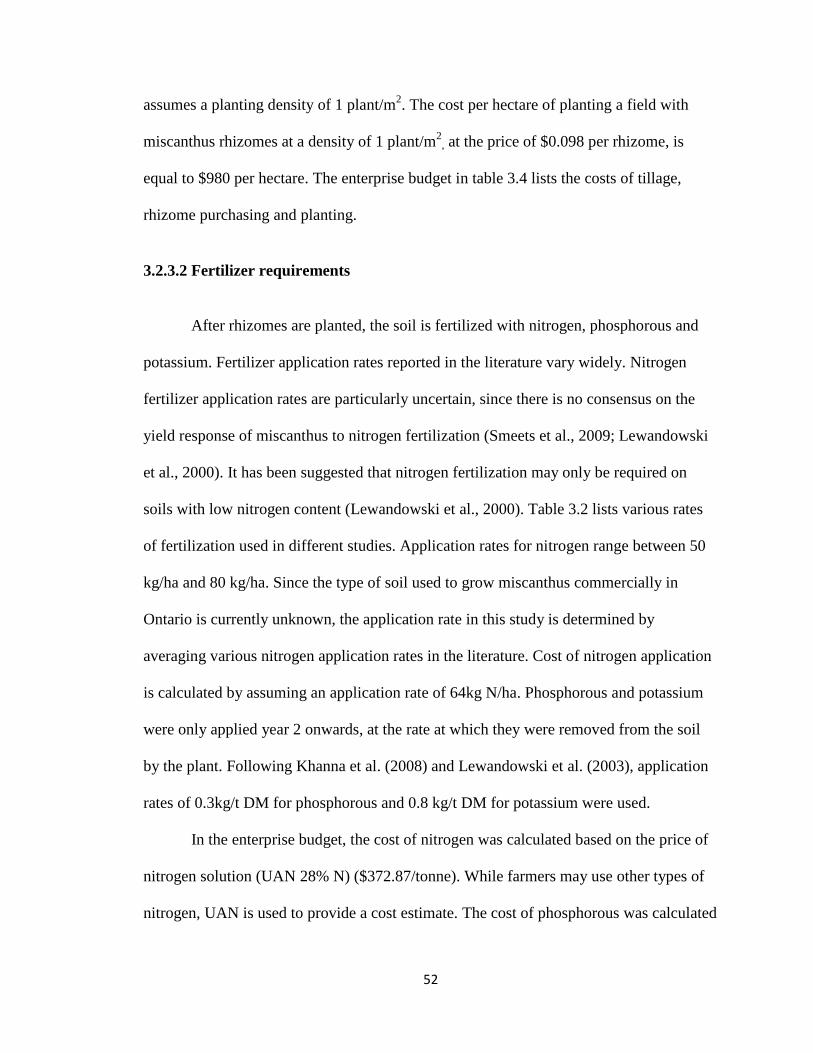
52

assumes a planting density of 1 plant/m2. The cost per hectare of planting a field with

miscanthus rhizomes at a density of 1 plant/m2

, at the price of $0.098 per rhizome, is

equal to $980 per hectare. The enterprise budget in table 3.4 lists the costs of tillage,

rhizome purchasing and planting.

3.2.3.2 Fertilizer requirements

After rhizomes are planted, the soil is fertilized with nitrogen, phosphorous and

potassium. Fertilizer application rates reported in the literature vary widely. Nitrogen

fertilizer application rates are particularly uncertain, since there is no consensus on the

yield response of miscanthus to nitrogen fertilization (Smeets et al., 2009; Lewandowski

et al., 2000). It has been suggested that nitrogen fertilization may only be required on

soils with low nitrogen content (Lewandowski et al., 2000). Table 3.2 lists various rates

of fertilization used in different studies. Application rates for nitrogen range between 50

kg/ha and 80 kg/ha. Since the type of soil used to grow miscanthus commercially in

Ontario is currently unknown, the application rate in this study is determined by

averaging various nitrogen application rates in the literature. Cost of nitrogen application

is calculated by assuming an application rate of 64kg N/ha. Phosphorous and potassium

were only applied year 2 onwards, at the rate at which they were removed from the soil

by the plant. Following Khanna et al. (2008) and Lewandowski et al. (2003), application

rates of 0.3kg/t DM for phosphorous and 0.8 kg/t DM for potassium were used.

In the enterprise budget, the cost of nitrogen was calculated based on the price of

nitrogen solution (UAN 28% N) ($372.87/tonne). While farmers may use other types of

nitrogen, UAN is used to provide a cost estimate. The cost of phosphorous was calculated

53

using the price for triple superphosphate 0-46-0 ($725.24/tonne) and the cost of

potassium was calculated using the price of Muriate of Potash 60% ($559/tonne).

Table 3.2: Fertilizer application rates post-establishment of miscanthus rhizomes

Study Fertilizers

N P K

Khanna et al., 2008 50 kg/ha 0.3 kg/t DM 0.8 kg/t DM

Lewandowski et al., 2000 60 kg/ha 0.3 – 1.1 kg/t DM 0.8 – 1.2 kg/t DM

Huisman et al., 1997 75 kg/ha 50 kg/ha 100 kg/ha

Heaton et al., 2003 80 kg/ha 10 kg/ha 60 kg/ha

Clifton-Brown, 2001 60 kg/ha 44 kg/ha 110 kg/ha

Himken et al., 1997 60 kg/ha 8 kg/ha 80 kg/ha

All prices were taken from the Ontario Farm Input Monitoring project (McEwan,

2009). A six year average (2005 – 2010) was used for all three fertilizers in the

enterprise budget. The final cost for nitrogen was $85.35/ha, while the costs for

phosphorous and potassium varied depending on yield. The cost of fertilizer application

using a fertilizer spreader was assumed to be $20/ha (OMAFRA, 2009).

3.2.3.3 Weed control

Once the land has been prepared and the rhizomes planted, it is important to

control any potential weed growth to ensure establishment of the poorly competing

miscanthus plants (Huisman et al., 1997). Herbicide application is only required during

the establishment phase (Smeets et al., 2009; Huisman et al., 1997; Styles et al., 2008).

The quantity and characteristics of control depend on the weeds in the field. In table 3.4,

herbicide costs are estimated based on application rates of Khanna et al. (2008). During

54

the pre-establishment period, 3.52 L/ha of Atrazine and 1.75 L/ha of 2, 4-D were applied.

The prices of herbicides are based on the Ontario Farm Input Monitoring project

(McEwan, 2009). The price of herbicides was averaged over six years (2005 to 2010).

The average price of Atrazine over this time span was $7.29/L and the average price of 2,

4-D over the same period was $8.09/L. The total herbicide cost equalled $39.86/ha

($25.70 Atrazine, $14.16 2, 4-D). The cost to apply the herbicides using a self propelled

applicator was taken from OMAFRA‘s 2009 custom rental rate survey.

3.2.3.4 Harvesting

Commercial harvesting of miscanthus typically happens in the spring of the third

year (second year yields), because the first year crop does not have significant yield.

Harvesting can commence when the crop has senesced (matured), however postponing

harvest until spring is a common practice because it improves the quality of the harvested

biomass. Harvesting of miscanthus is carried out using a conventional disc mower and

baler that delivers large bales (Khanna et al., 2008). This study calculates harvesting costs

for all three scenarios using the conventional mowing and baling system.

Baling of miscanthus is possible using all kinds of balers. Round bales will give a

baled dry matter density of about 130 kg/m3, and rectangular ―big bales‖ are about 150

kg/m3 (Venturi et al., 1998; Lewandowski et al., 2000). Cost estimates for this study are

based on miscanthus being mowed and then baled. In table 3.4, mowing costs are

estimated to be $42.5/ha (OMAFRA, 2009). Since harvesting costs are partly dependent

on yield, mowing and raking costs could be underestimated. This is because they are

based on the cost of producing hay which has 40- 50% less yield than miscanthus

55

(OMAFRA, 2006). It is difficult to estimate the increase in harvesting costs due to

increase in yield because the total cost of harvesting does not increase proportionately

with yield (Khanna et al., 2008). In fact, the per-tonne cost of harvesting falls as

harvested yield increases due to the presence of fixed costs per hectare of mowing

(Khanna et al., 2008). Based on the field trial experience in Ontario, raking of miscanthus

is only required if it has been rained on prior to baling. Hence the cost of raking is not

included in the enterprise budget (table 3.4).

Once the crop has been raked it needs to be baled for storage and transportation.

To estimate the cost of baling miscanthus, this study used the cost of production budget

for hay available from OMAFRA (2006). It is assumed that large square bales with a

density of 218 kg/m3 will be produced, and each bale will weigh 334 kg (OMAFRA,

2006). This will allow 3 bales to be produced from each tonne of miscanthus. With a

yield of 14t/ha, 42 bales will be produced per hectare. Since the cost per bale is $7, the

total baling cost per hectare of miscanthus is $294 (OMAFRA, 2006). The bales are then

transported to a storage facility at a price of $1.37/bale, which includes loading the bales

onto a truck, transporting the bales to the storage facility and then unloading the bales

(OMAFRA, 2006). The total cost incurred to transfer a hectare of miscanthus from field

to storage is $57.54 for a yield of 14t/ha.

3.2.3.5 Storage

To ensure year round availability of biomass for heating, it is important to consider

the costs of storage. Standard methods for straw or hay can be used for collecting and

56

handling miscanthus bales for transport and storage. Several storage methods are

available:

1) Storage in open air without covering

2) Storage in open air with a plastic sheeting cover

3) Storage in existing or new farm buildings

The cheapest and most used option is storage in open air with plastic sheeting

(Huisman et al., 1997). Storage in new buildings is prohibitively expensive unless

existing buildings are used, but they may not be available (Huisman et al., 1997). Storage

in open air is problematic due to loss of biomass from decay (Smeets et al., 2009). This

study assumes storage of miscanthus square bales in open air, covered with plastic

sheeting. In the enterprise budget the cost per hectare of storing miscanthus changes with

the yield. The total storage cost per tonne of miscanthus is estimated to be $4.50

assuming 3 bales/tonne are produced. The storage cost per bale is assumed to be $1.50

(OMAFRA, 2010a)

3.2.4 Net Present Value

Net present value (NPV) is the time value of money and is calculated by

discounting all future values of costs and revenues by an appropriate discount rate to

determine the present value of the enterprise. If the value of NPV is positive, the

enterprise would make a profit, a negative value would represent a loss and a zero value

would indicate a breakeven position. The following formula can be used to calculate the

NPV of a 20 year miscanthus enterprise:

57

(1)

Where NPV is the net present value of net returns, t is the time period in years; Rt is the

total revenues earned in dollars in time t; Ct is the total costs incurred in dollars in time t

and i is the discount rate.

In equation (1) the discount rate i is the time value of money based on the level of

risk involved in an investment. A high risk investment would have a higher discount rate

and would place a lower value on future cost and revenue streams than a low risk

investment. Based on the above formula, a higher t value would result in a higher

denominator which in turn will result a lower numerator value i.e. lower R and C. In

other words, a dollar earned/spent in year 1 will have a higher value than a dollar

earned/spent in year 20. In table 3.4 the total cost incurred is a constant $905.39 from

year 3 to 20. However, the discounted value of $905.39 spent in year 3 is $782.11; year 4

is $744.86 and so on. It is noted from table 3.4 that discounted cost value decreases as t

increases. Similarly, revenue streams R will be lower as t increases from year 3 to year

20.

In case of the miscanthus enterprise the discount rate directly affects the

breakeven price of miscanthus. As the discount rate increases the breakeven price

increases because increasing the discount rate decreases the value of net revenues

(revenue –cost) that are received from year 2 onwards while the establishment costs

incurred in year 1 stays the same. In the literature, the discount rate for a miscanthus

enterprise budget ranges from 4% to 7% (Khanna et al., 2008; Styles et al., 2008;

Huisman et al., 1997). Following Styles et al (2008) the base case scenarios assume a

58

discount rate of 5%. The impact of discount rate on the results is also examined in the

sensitivity analysis.

Since this study is trying to determine the breakeven price of growing miscanthus for

a farmer, NPV would need to equal zero. This can also be achieved if the NPV of all

input costs, over the 20 year enterprise, would equal the NPV of all revenue received over

the same period. Equation (2) demonstrates this equality

(2)

Where ― ‖ is the discounted revenue per hectare over the 20 year period and

― ‖ is the discounted input costs per hectare over the 20 year period.

The NPV of costs per hectare for each year can be calculated by summing up all input

costs incurred in each year and discounting it by the discount rate. To calculate the NPV

of revenues, market price per tonne of miscanthus (in each year) would have to be

multiplied by the yield per hectare and then discounted by the discount rate as in equation

(3)

(3)

Where P is the market price per tonne of miscanthus and yield is the quantity of

miscanthus produced per hectare.

Since the market price of miscanthus is not known, the yield per hectare can be

discounted over the 20 year period and used as a proxy for revenue. Hence equation (2)

can be rewritten as equation (4)

59

(4)

Where NPV (yield) is the discounted yield per hectare over the 20 year period

Therefore, the breakeven price per tonne of miscanthus is calculated by dividing the

discounted cost by the discounted yield as shown in equation (5) and (6)

(5)

(6)

Furthermore, if the achieved breakeven price is multiplied by the discounted yield to

obtain discounted revenue, then the discounted revenue will equal discounted cost which

results in zero NPV (i.e. breakeven position).

3.2.5 Opportunity Cost

As mentioned in chapter 2, studies estimating the cost of growing miscanthus

usually do not include the cost of land (Huisman et al., 1997; Styles et al., 2008; Venturi

et al., 1998). However, land cost is an important factor in calculating the breakeven price

of growing miscanthus. Land cost can be calculated by either using the rental rate of farm

land or by calculating the opportunity cost of land. Most land rental rates in Ontario are

established by using local market rates, which reflect the supply of and demand for rental

land in a local area (Gamble, 2001). The rental rate of land can be calculated using

various methods, such as the current market approach, landlords cost approach, crops

share equivalent approach, income approach or the contribution approach (Gamble,

60

2001). However, no survey has been done in Ontario that follows the rental rate of land.

Since this data is not available the opportunity cost of land was used to estimate the cost

of land in this study. Opportunity cost is estimated as the foregone profits from the next

best alternative use of the land that is converted, to miscanthus production. Since corn,

soybeans, barley, wheat and hay are the dominant crops grown in Ontario, opportunity

costs for farm land in Ontario is calculated based on the net revenues of these three crops

(McGee, 2011). The net revenues are calculated by deducting the cost per hectare

(OMAFRA, 2011a) from the gross farm receipts (OMAFRA, 2011b). The net revenue for

the crops range from $30/ha to $389.93/ha. To calculate the average return per hectare,

various kinds of corn, soybean and wheat were included. Table 3.3 lists different crops

used to calculate the average. An average price of $245.82/ha was estimated to be the

opportunity cost of land in Ontario.

3.2.6. Comparison to other studies

Table 3.5 compares the cost of production estimates of this study to the estimates

made by Khanna et al. (2008). Since all estimates made by Khanna et al. (2008) were in

U.S. dollars for the year 2003, the U.S. dollar values were converted to Canadian dollars

through multiplying them by 1.401. The appropriate inflation rate was then applied to

give all values in 2009 prices. The conversion and inflation rates were based on the rates

provided by the Bank of Canada (2010).

61

Table 3.3: Average net returns per hectare for corn, soybean, barley, wheat and hay

for Ontario from 2005 to 2009

Crop Net returns per hectare ($/ha)

Soft winter wheat – conventional $235.75/ha

Soft winter wheat – no till $284.75/ha

Hard red winter wheat – conventional $201.50/ha

Hard red winter wheat – no till $250.13/ha

Barley $64.70/ha

Grain corn – conventional $315.70/ha

Grain corn – minimum till $344.70/ha

Grain corn – no till $330.70/ha

Soybean – conventional $347.18/ha

Soybean – no till $346.55/ha

Soybean – roundup ready $389.93/ha

Hard red spring wheat $30.00/ha

Alfalfa - Timothy Hay $54.63/ha

Average opportunity cost of farmland in

Ontario $245.82/ha

Source: Returns per hectare for every crop was taken from OMAFRA, 2010. Accessed

from: http://www.omafra.gov.on.ca/english/busdev/facts/pub60.htm#2010 and

http://www.omafra.gov.on.ca/english/stats/crops/index.html

62

Table 3.4: Cost of production budget for miscanthus, base case for scenario 1 ($/ha).

Cost item/ ha Year 1 Year 2

Year 3

– 20 Sum (20 yrs)

Rhizomes 980.00 0.00 0.00 980.00

Establishment

Primary tillage – Disc 40.00 0.00 0.00 40.00

Secondary tillage – Harrowing 20.00 0.00 0.00 20.00

Potato planter 75.75 0.00 0.00 75.75

Herbicide

2, 4D-B 14.16 0.00 0.00 14.16

Atrazine 25.66 0.00 0.00 25.66

Application equipment

Self propelled/with GPS 22.50 0.00 0.00 22.50

Fertilizer

Nitrogen 85.35 85.35 85.35 1,706.92

Phosphorousa 0.00 3.30 6.59 121.99

Potassiuma 0.00 5.21 10.42 192.70

Airflow/Fertilizer spreader

Spread dry fertilizer 20.00 20.00 20.00 400.00

Harvesting

Mowing 0.00 42.50 42.50 807.50

Bailing a 0.00 147.00 294.00 5,439.00

Staging and loading

Load, transport, unload a 0.00 28.77 57.54 1,064.00

Storage a 0.00 31.50 63.00 1,165.50

Opportunity cost 245.82 245.82 245.82 4,916.40

Total cost 2,019.23 609.44 825.22 17,482.57

Discounted cost (Discount rate 5%)b 1,923.08 552.78 678.91

c 11,225.46

Delivered yield discounted at 5% (t/ha)b 0.00 5.90 11.25

d 143.95

Breakeven farm-gate price ($/t) 77.98 a

Costs change with yield of miscanthus stand. b NPV formulas applied, values depend on the year (t).

c The nominal total cost for year 3 to 20 is the same ($905.39), however applying the

NPV formula changes the real cost for every year. Complete budget can be found in

appendix A. d

The yield for year 3 to 20 is the same, however since yield is used as a proxy for

revenue it is discounted and changes for every year according to the NPV formula.

63

The cost estimates made by this study are very similar to the estimates made by

Khanna et al. (2008). The greatest discrepancies arise in the rhizome cost per hectare and

harvesting cost per hectare. The difference in the rhizome cost per hectare is a result of

different unit prices. The cost per rhizome used by Khanna et al. (2008) was not used by

this study, rather an average of the various rhizome prices found in the literature was

calculated. The estimate used by Khanna et al. (2008) was considered too low for this

study since a market for miscanthus does not currently exist in Ontario. Harvesting cost

differences between the two studies can be explained by two factors. First, the yield used

by Khanna et al. (2008) (27.85t/ha) is almost double the yield used by this study (14t/ha).

Increasing the yield would increase harvesting costs. Second, this study based its

harvesting estimates on the cost of harvesting and storing hay which has 40%-50% less

yield than miscanthus (OMAFRA, 2006). Hence, harvesting costs from this study could

be an underestimation. The higher yield used by Khanna et al. (2008) also explains the

higher establishment costs estimated in that study. Finally, the differences in herbicide

and fertilizer costs are a result of different chemical prices in Canada and the U.S.

(McEwan, 2010).

64

Table 3.5: Cost of production estimate comparison ($/ha).

Khanna et al., 2008 This study

Item Cost ($/ha) Assumptions Cost ($/ha) Assumption

Rhizomes $519.23/ha

Cost per rhizome was

$0.06. Rhizomes were

planted at a density of

1 rhizome/m2

$980/ha

Cost per rhizome was

$0.098. Rhizomes were

planted at a density of 1

rhizome/m2

Establishment $164.04/ha

Includes cost of

disking, harrowing

and planting rhizomes

using a potato planter.

$135.75/ha

Includes cost of

primary and secondary

tillage and planting

rhizomes using a potato

planter

Herbicide $39.63/ha

Applied 3.5 L/ha of

Atrazine and 1.75L/ha

of 2,4-D. Cost of

application included

$62.32/ha

Applied 3.5 L/ha of

Atrazine and 1.75L/ha

of 2,4-D. Cost of

application included

Fertilizer $83.34/ha

Applied 50kg N/ha

along with potassium,

phosphorous and lime.

Cost of application

included.

$122.36/ha

Applied 64 kg N/ha

along with

phosphorous and

potassium. Cost of

application included.

Harvesting $1271/ha

Includes cost of

mowing, raking

bailing, loading and

storage for a yield of

27.85t/ha at 20%

moisture

$520/ha

Includes cost of

mowing bailing,

loading and storage for

a yield of 14t/ha at 20%

moisture

65

3.3 Sensitivity Analysis

The breakeven price of the base scenarios is based on a number of assumptions.

Yield of the stand is assumed of be 14t/ha (20% moisture content), rhizome cost is

assumed to be $0.098 per rhizome, discount rate is assumed to be 5%, and harvesting is

assumed to be carried out using the mowing and baling method. The following sections

shall justify the need for a sensitivity analysis for each of the assumptions and discuss the

reason for the range of values used for every assumption. Section 3.3.1 outlines the need

for a sensitivity analysis for the yield of the stand; section 3.3.2 reviews the need for a

sensitivity analysis of the cost per rhizome, section 3.3.3 focuses on the sensitivity

analysis of the discount rate and section 3.3.4 explains the need for a sensitivity analysis

of the harvest method.

3.3.1 Yield of a miscanthus stand

It is important to conduct a sensitivity analysis on the yield of miscanthus, as

yield can have a significant effect on the per tonne breakeven price of miscanthus

production. Since the cost per hectare of the inputs required for producing miscanthus

stays the same irrespective of the yield (except for some fertilizer quantities, harvesting

and storage), the breakeven price of a stand with high yields will be lower than the

breakeven price of a stand with low yields. Sensitivity analysis of the yield is also

necessary because the actual yield of a miscanthus stand in Ontario is unknown. Since

stand yield is affected by soil type and weather conditions, different sites within Ontario

could have different yields. A sensitivity analysis can provide an insight into the effects

of such variation on the breakeven price.

66

In the literature yield of a stand of miscanthus ranges from 3.1 t/ha to 37.7 t/ha

(see table 3.1). A wide range in yield exists due to different genotypes and climatic

conditions of each study. Since none of these studies have been conducted in Ontario it is

unknown which miscanthus genotype would survive best under Ontario environmental

conditions. There is no easy way to compare Ontario soils and climate to that of other

countries to estimate miscanthus yields. Sensitivity analysis with regard to yield will

provide a range of breakeven prices that miscanthus growers can expect in Ontario.

Yield values used for the sensitivity analysis range from 7t/ha to 21t/ha (20%

moisture content) to cover different soil types and temperatures in Ontario. This range is

50% above and below the average yield used in the base case scenarios. The range is

picked for a number of reasons. First, a yield higher than 21t/ha is considered to be

unreasonable under Canadian conditions. A review of the literature indicates that any

studies that report a miscanthus yield greater than 21t/ha (20% moisture content) were

conducted in areas with climates warmer than the Canadian climate, such as Turkey or

Illinois (Acaroglu et al., 2005; Khanna et al., 2008). It is unreasonable to expect

miscanthus to grow as vigorously in Canada as it does in the warmer climates because the

harsh winters adversely affect miscanthus yield. Warm temperatures are required for

higher yield production in the stand (Farrell et al., 2006). However, since the warm

temperatures (spring and summer) only last a few months in Ontario, the growing season

is shortened by cool temperatures and frost in the winter, reducing the overall yield of the

stand. Secondly, yields lower than 7t/ha (20% moisture content) have not been

considered because current trial plots of miscanthus around Ontario have yields higher

than 7t/ha (20% moisture content). The Ontario trials use the genotypes Nagara, Amuri

67

and two different Giganteus genotypes (M1 select, T. Select and Polish). The plants are

grown on three different types of soil - silt loam, clay loam and loam. Additionally, since

these stands are only in their second year, it can be assumed that their peak yields will be

greater than 7t/ha (20% moisture content).

3.3.2 Rhizome cost

The largest establishment cost for a miscanthus grower is the purchasing of

rhizomes in the first year. According to the base case scenarios, if the cost per rhizome

equalled $0.098, a grower would spend $980 per hectare on rhizomes in the first year.

Therefore a change in rhizome price can influence the breakeven price. In the literature,

rhizome costs range from $0.03 per rhizome to $0.60 per rhizome, depending on the

method of production (Smeets et al., 2009; Khanna et al., 2008; Lewandowski et al.,

2000; Atkinson et al., 2009; Heaton et al., 2004). Currently there is only one known

commercial rhizome producer in Canada and their prices range from $0.27 per rhizome to

$0.70 per rhizome, depending on the quantity bought (New Energy Farms, 2010). Since a

competitive market for miscanthus does not yet exist in Canada, New Energy Farms is

expected to be making above normal profits, and their prices are not believed to be

reflecting the price a miscanthus grower would pay for rhizomes in a competitive market.

Even though Canadian rhizome prices are available from New Energy Farms ($0.27 -

$0.70), the literature range of $0.03 per rhizome to $0.60 per rhizome is used for the

rhizome cost sensitivity analysis. This is done because the cost of rhizomes is expected to

be lower in a competitive market as a result of competition and innovation of rhizome

production techniques.

68

3.3.3 Harvest method

The base case scenarios used the mowing and baling harvest method. Venturi et

al. (1997) suggest that a forage harvester used for harvesting silage maize or grass can

also be used for harvesting miscanthus. This method of harvesting does not require

miscanthus to be mowed or raked prior to storage. Using a forage harvester can lead to

potential savings, since one machine carries out all the different activities and therefore

greatly cuts down on labour costs. A self-propelled forage harvester chops the crop into

small pieces. The chopped material is then hauled to the storage site where it is stored

either in a storage silo, silage bunker, silage bags or simply in a pile. For the harvest

method sensitivity analysis, the base case breakeven prices are recalculated using the

forage harvester method. The cost for the forage harvester is obtained from OMAFRA‘s

provincial survey of custom farm work charged in 2006. The cost includes storage costs

and is based on the cost of chopping, hauling, blowing and packing corn silage. The total

cost per hectare is $233.75. This price was determined by converting the cost per hour

rate ($561/hour) charged by a contractor. On average a contractor could harvest 2.4

hectares of corn silage in one hour.

3.3.4 Discount rate

As mentioned earlier a miscanthus enterprise can last up to 20 years. Therefore,

the costs and revenues of the enterprise need to be discounted to determine the Net

Present Value (NPV). The base case NPV is calculated using a 5% discount rate. Usually

the discount rate for an enterprise is determined by its level of riskiness, where the riskier

the enterprise, the higher the discount rate. Khanna et al. (2008) used a discount rate of

69

4%, Styles et al. (2008) used a discount rate of 5% and Huisman et al. (1997) used a

discount rate of 7% to calculate their NPV. Since a market for miscanthus does not

currently exist in Ontario, a number of uncertainties surround this enterprise, such as the

cost of production, market price, supply, demand etc. The miscanthus enterprise is

considered to be a high risk investment due to this uncertainty. However, as the market

for miscanthus develops the uncertainly will decreases and investing in miscanthus will

not be considered as high risk. To evaluate various levels of risk involved, a discount rate

range from 4% to 10% is applied in the sensitivity analysis. This range includes all the

discount rate values used in previous studies and sufficiently captures the various levels

of uncertainty.

3.4 Chapter summary

To analyse the economic performance of miscanthus in Ontario, it is important to

determine the feasibility of this crop from a production standpoint for Ontario crop

producers, as well as from a consumption standpoint as an energy source for the

greenhouse industry in Ontario. Farmers in Ontario will only produce miscanthus if they

make a profit which is greater than, or equal to, the profit they make with their current

crops, and the greenhouse industry will only demand miscanthus if its market price is less

than, or equal to, the price of fuels they currently use. To determine if miscanthus would

be an attractive energy crop for the farmers as well as the Ontario greenhouse industry, it

is important to determine the breakeven price of producing miscanthus.

Since miscanthus has not been produced commercially in Ontario, an enterprise

budget is created to determine the breakeven price of miscanthus. Assumptions regarding

70

the stand life cycle, yield, rhizome cost, harvest method and discount rates are made. The

stand is assumed to be fully established in the first 3 years, and survive for 20 years.

Rhizomes are assumed to cost $0.98/rhizome and the stand is expected to yield 14 t/ha

when harvested. The stand is harvested using the mow and bale method and the entire

enterprise budget is discounted at a rate of 5%. Cost of inputs, harvest method and

storage are taken from OMAFRA. The cost of production estimated by this study is

compared to the cost estimates presented by Khanna et al. (2008).To determine the effect

of assumptions on the breakeven price of miscanthus, a sensitivity analysis with regards

to yield, rhizome cost, harvest method and discount rate is undertaken. To determine the

effect of the stand life cycle on the breakeven price, three different stand life cycle

scenarios are considered.

The next chapter outlines the results of the base case scenarios as well as the

results of sensitivity analysis performed on various assumptions. Effects of these

assumptions on the breakeven price are analyzed. The results are followed by a

discussion that compares the cost of using miscanthus as a source of bioenergy to other

sources of energy. It also attempts to determine the greenhouse industry‘s willingness to

pay for energy produced from miscanthus.

71

Chapter 4: Results and Discussion

This chapter begins by presenting results of the three base case scenarios as well

as results of the sensitivity analysis. The sensitivity analysis evaluates effects of four

major assumptions on the breakeven price of the base case scenarios. The assumptions

that are evaluated are yield of the stand, rhizome cost, harvest method and the discount

rate. The results are followed by a discussion that attempts to determine the greenhouse

industry‘s willingness to pay by comparing the cost of energy produced from miscanthus

to the cost of energy from other fuels. This comparison will help determine if miscanthus

producers would make a profit, loss or break even by producing and selling miscanthus in

a competitive market. The potential net revenues from miscanthus are also compared to

the expected net revenues of other Ontario crops to determine if Ontario farmers would

be willing to produce miscanthus.

4.1 Results

This section reports the breakeven price for the base scenarios as well as results of

the sensitivity analysis. Three scenarios are evaluated for the base case as well as for the

four sensitivity factors. The three scenarios are best case, delayed peak yield

establishment and early termination, and refer to the life cycle of a miscanthus stand since

the actual life cycle of the stand is unknown. In the best case scenario the stand is

assumed to reach its peak yield in three years and has a productive life of 20 years. In the

delayed peak yield establishment scenario the stand takes five years to reach peak yield

and stays at peak yield for 20 years. Finally, in the early termination scenario the stand

reaches peak yield in three years but its use is terminated in year 12. It should be noted

72

that in any given analysis only the value of one assumption is altered. The values of all

other assumptions stay the same.

4.1.1 Base case results

The breakeven prices for the three base case scenarios are listed in table 4.1. The

breakeven price for miscanthus, before including the opportunity cost of land, is $53.46

per tonne in the best case scenario, $55.33 per tonne in the delayed peak yield

establishment scenario and $57.78 per tonne in the early establishment scenario. Delayed

peak yield establishment increases the breakeven price by $1.87 per tonne, which is

relatively small compared to the increase of $4.32 per tonne due to early termination.

After including the opportunity cost of land the breakeven price for miscanthus increases

to $77.98 per tonne in the best case scenario, $82.11 in the delayed peak yield

establishment scenario and $85.03 per tonne in the early termination scenario. Including

the opportunity cost of land increases the breakeven price for the best case scenario by

46%, the delayed peak yield establishment scenario by 48% and the early termination

scenario by 47%. Since the total stand yield in every scenario is different, applying a

fixed opportunity cost affects each scenario to a varying degree.

Table 4.1: Breakeven price for the base case of all three scenarios

Best case Delayed peak yield

establishment Early termination

Breakeven price

($/tonne) $53.46/t $55.33/t $57.78/t

Breakeven price

with opportunity

cost ($/tonne)

$74.74/t $78.57/t $80.22/t

Yield= 14 t/ha, rhizome cost = 0.098, discount rate = 5% and crop was harvested using

the mow and bale method

73

4.1.2. Yield sensitivity results

The base case used a yield of 14 t/ha for all three scenarios. A yield range of 7t/ha

(20% moisture content) to 21t/ha (20% moisture content) was used for the sensitivity

analysis. Figure 4.1 shows the change in the breakeven price as the yield of the stand

changes while keeping all other variables at base case values. As the yield of the stand

increases in all three scenarios the breakeven price decreases. This trend is similar to the

trend found by Khanna et al. (2008). Additionally, a 50% decrease in yield from the base

case has a greater effect on the breakeven price than a 50% increase in yield from the

base case for all three scenarios. For the best case scenario when yield decreases from 14

t/ha (20% moisture content) to 7t/ha (20% moisture content), the breakeven price

increases by 55.65% to $116.33/t. However when the yield increases to 21t/ha (20%

moisture content) the breakeven price decreases by 22.78% to $60.87/t compared to the

base scenario breakeven price of $74.74/t. For the delayed peak yield establishment

scenario the breakeven price increases by 57.82% ($124/t) when the yield decreases from

14 t/ha to 7 t/ha, and the breakeven price decreases by 23.86% ($63.43/t) when the yield

is increased to 21 t/ha from the base case yield. Finally, for the early establishment

scenario the breakeven price increases by 58.67% ($127.29/t) when the yield is decreased

to 7t/ha (20% moisture content), and the breakeven price decreases by 24.31% ($64.53/t)

when the yield is increased to 21 t/ha (20% moisture content) from 14 t/ha (20% moisture

content). The reason the breakeven price decreases with increase in yield for all three

scenarios is because the cost per hectare of growing miscanthus (except for harvesting

and storage costs) stays the same, irrespective of the yield. As the yield increases the cost

per hectare gets divided by a bigger number, thereby decreasing the cost per tonne.

74

Another trend apparent from figure 4.1 is that at higher yields the difference

between the breakeven prices for all three scenarios is significantly less. At 7 t/ha (20%

moisture content) the difference in breakeven price between the best case and delayed

peak yield establishment scenario is $7.67, while the difference between the best case and

the early termination scenario is $10.96. However, at 21 t/ha (20% moisture content) the

difference between the best case and the delayed peak yield establishment scenario is

reduced to $2.56, while the difference between the best case and the early termination

scenario is reduced to $3.65. Since higher yields result in higher revenues the losses

incurred by delayed peak yield establishment or early termination are reduced, decreasing

the monetary effect of these phenomena.

Figure 4.1 Change in breakeven price as yield of a miscanthus stand changes

Rhizome cost = 0.098, discount rate = 5% and crop was harvested using the mow and

bale method

60.00

70.00

80.00

90.00

100.00

110.00

120.00

130.00

140.00

7 8 9 10 11 12 13 14 15 16 17 18 19 20 21

Bre

ak

even

pri

ce (

$/t

on

ne)

Yield (tonne/ha)

Best case

Delayed peak

yield

establishment

Early

termination

75

4.1.3 Rhizome cost sensitivity results

The cost per rhizome was assumed to be $0.098 in the base case scenarios. The

sensitivity analysis tested a price range of $0.03 per rhizome to $0.60 per rhizome. Figure

4.2 shows the change in breakeven price as the cost per rhizome changes while keeping

all other variables at base case values. Increasing the price per rhizome from

$0.03/rhizome to $0.60/rhizome increases the breakeven price of the best case scenario

from $70.24/tonne to $107.95/tonne. The breakeven price for the delayed peak yield

establishment scenario increases from $73.66/ tonne to $114.84/tonne, and the breakeven

price for the early termination scenario increases from $73.55/tonne to $129.46/tonne.

Unlike the other variables, there is a linear relationship between the breakeven price and

the rhizome cost. This linear relationship is caused by the fact that the cost is only

incurred in the first year and is not discounted over time. For every cent increase in

rhizome cost, the breakeven price increases by $0.66 in the best case scenario, $0.72 in

the delayed peak yield establishment scenario and $0.98 in the early termination scenario.

Rhizome costs affect the early termination scenario the most and affect the best case

scenario the least. This difference in effect of the rhizome cost on the different scenarios

can be explained by the total yield produced over the entire life of the stand. The total

rhizome costs incurred in year one is divided by the total biomass yield produced by a

stand over its life time. Therefore, for the same yield per hectare, the early termination

scenario will produce the least amount of biomass since the productive stand life is only

12 years. The delayed peak yield establishment scenario will produce more biomass than

the early termination scenario due to its 20 year life, however due to the delay in

achieving peak yield it produces less biomass than the best case scenario. Hence, increase

76

in rhizome cost will have the greatest monetary effect on the early termination scenario

(least total biomass yield) and the least monetary effect on the best case scenario

(maximum total biomass yield).

Figure 4.2: Change in breakeven price as the cost per rhizome changes

Yield= 14 t/ha, discount rate = 5% and crop was harvested using the mow and bale

method

4.1.4 Harvest method sensitivity results

The base case scenarios assumed that miscanthus will be harvested using the mow

and bale method since it is the more commonly used method of harvesting crops. To

assess the effect of a different harvest method on the breakeven price, the method of

forage harvesting was used for the sensitivity analysis. Table 4.2 lists the breakeven price

for all three scenarios for the two different harvest methods while keeping all other

variables at base case values. Using a forage harvester decreases the breakeven price in

all three scenarios. The breakeven price decreases by $19.79 for the best case scenario, by

70.00

80.00

90.00

100.00

110.00

120.00

130.00

0.0

3

0.0

9

0.1

5

0.2

1

0.2

7

0.3

3

0.3

9

0.4

5

0.5

1

0.5

7

Bre

ak

even

pri

ce (

$/t

on

ne)

Cost of rhizome ($/rhizome)

Best case

Delayed peak yield

establishment

Early termination

77

$18.64 for the delayed peak yield establishment scenario and by $21.07 for the early

termination scenario. Using a forage harvester decreases the breakeven price per tonne of

miscanthus significantly.

Table 4.2 Breakeven prices for two types of harvest methods.

Harvest method

Breakeven price ($/tonne)

Best case Delayed peak yield

establishment

Early termination

Mow and Bale $74.74/tonne $78.57/tonne $80.22/tonne

Forage Harvester $58.19/tonne $63.43/tonne $63.96/tonne

Yield= 14 t/ha, rhizome cost = 0.098 and discount rate = 5%

4.1.5 Discount rate sensitivity results

A discount rate of 5% was used for the base case scenarios. A sensitivity analysis

on the discount rate was done using the range of 4% to 10%. Figure 4.3 shows the change

in breakeven price for all three scenarios as the discount rate changes while keeping all

other variables at base case values. For all three scenarios, as the discount rate increases

the breakeven price increases. This happens because increasing the discount rate

decreases the value of net revenues (revenue – cost) that are received from year 2

onwards. However the establishment costs incurred in year 1 stay the same. Figure 4.3

shows the increase in breakeven price for the three scenarios as discount rate changes

from 4% to 10%. Breakeven price for the delayed peak yield establishment scenario

increases by 11% from $77.30/t to $85.91/t. The best case scenario breakeven price

78

increase by 8% ($73.81/t to $79.97/t) and the early termination scenario breakeven price

increases by 7% ($79.32/t to $85.10/t).

Figure 4.3 Change in breakeven price as the discount rate increases

Yield= 14 t/ha, rhizome cost = 0.098 and crop was harvested using the mow and bale

method

4.2 Discussion

The cost of growing miscanthus in Ontario ranges from $35.83/t to $127.29/t

(includes opportunity cost of land) depending on the yield of the stand, life cycle of the

stand, cost per rhizome, method of harvest and discount rate. Table 4.3 shows the effect

of a 50% increase or decrease of the various variables on the breakeven price of

producing miscanthus. To identify which variables have the greatest effect on the

breakeven price, it is important to change all variable by the same amount (50%). In

general, the breakeven price increases when stand yield decreases, rhizome cost increases

70.00

72.00

74.00

76.00

78.00

80.00

82.00

84.00

86.00

88.00

90.00

4% 5% 6% 7% 8% 9% 10%

Bre

ak

even

pri

ce (

$/t

on

ne)

Discount rate (%)

Best case

Delayed peak

yield

establishment

Early

termination

79

and discount rate increases. Conversely, the breakeven price in all three scenarios

decreases when stand yield increases, cost per rhizome decreases, discount rate decreases

and the forage harvester method of harvesting is used. Yield and harvest method have the

greatest effect on breakeven price in all three scenarios. Decreasing stand yield by 50%

(7t/ha) increases the breakeven price for the best case scenario by 55.65% ($116.33/t),

increases the breakeven price for the delayed peak yield establishment scenario by

57.82% ($124/t) and increases the breakeven price for the early termination scenario by

58.67% ($127.29/t). Increasing stand yield by 50% (21t/ha) decreases the breakeven price

for the best case scenario by 22.78% ($60.87/t), decreases the breakeven price for the

delayed peak yield establishment scenario by 23.86% ($63.43/t) and decreases the

breakeven price for the early termination scenario by 24.31% ($64.53/t). Switching

harvest method to forage harvesting decreases the breakeven price by 28.44% ($58.19/t)

in the best case scenario. The breakeven price of the delayed peak yield establishment

scenario is reduced by 23.86% ($63.43/t) and the early termination scenario breakeven

price is reduced by 25.42% ($63.96/t).

The breakeven price of growing miscanthus calculated from this study is

compared to the breakeven prices determined by Styles et al. (2008), Venturi et al. (2003)

and Khanna et al. (2008) in table 4.4. The base case breakeven price of $74.74/t to

80.22/t estimated in this study falls within the range suggested by Khanna et al. (2008)

($63.59/t – $89.96/t). Changing the harvest method to chopped (using a self-propelled

forage harvester) from baled decreases the breakeven price range to $58.19/t to $71.28/t,

which is at the upper end of the range $55.56/t to $72.09/t reported by Styles et al. (2008)

that assess the effect of different supply chains on the breakeven price of miscanthus.

80

Table 4.3: Sensitivity of breakeven prices

Best case Delayed peak yield

establishment

Early

termination

Base Case1 $74.74/tonne $78.57/tonne $80.22/tonne

Price

($/t)

%

Change

Price

($/t)

%

Change

Price

($/t)

%

Change

50% decrease in

miscanthus yield (7t/ha) 116.33 55.65% 124.0 57.82% 127.29 58.67%

50% increase in

miscanthus yield (21

t/ha)

60.87 -22.78% 63.43 -23.86% 64.53 -24.31%

50% decrease in

rhizome cost

($0.049/rhizome)

71.50 -4.53% 75.03 -4.71% 75.41 -6.37%

50 % increase in

rhizome cost

($0.147/rhizome)

77.98 4.33% 82.11 4.50% 85.03 5.99%

50% decrease in

discount rate (2.5%) 72.50 -3.08% 75.51 -4.05% 78.03 -2.80%

50% increase in

discount rate (7.5%) 77.23 3.33% 82.04 4.41% 82.58 2.94%

Forage harvester 58.19 -28.44% 63.43 -23.86% 63.96 -25.42%

% Change is calculated relative to the breakeven prices in the base case 1 For the base case yield= 14 t/ha, rhizome cost = 0.098, discount rate = 5% and crop was

harvested using the mow and bale method.

Decreasing the yield to 7t/ha and increasing cost per rhizome to $0.60 in the

sensitivity analysis, increases the breakeven price range to $104.88/t - $129.46/t. This

price range is higher than the breakeven suggested by Khanna et al. (2008) as well as

Styles et al. (2008).This discrepancy can be explained by the fact that neither Khanna et

al. nor Styles et al. conducted a sensitivity analysis regarding rhizome cost. Also while

Khanna et al. did assess the effect of a 25% yield reduction on the breakeven price, the

base yield in the study was 20t/ha and a 25% reduction in yield (15 t/ha) was still much

higher than the yield of 7t/ha considered in this study. Finally, the breakeven price of this

study is significantly greater than the breakeven price suggested by Venturi et al. (2003)

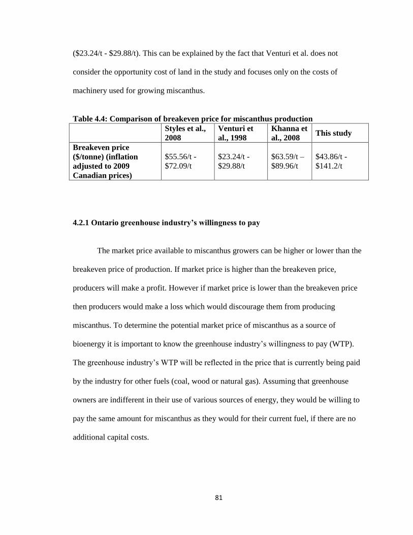
81

($23.24/t - $29.88/t). This can be explained by the fact that Venturi et al. does not

consider the opportunity cost of land in the study and focuses only on the costs of

machinery used for growing miscanthus.

Table 4.4: Comparison of breakeven price for miscanthus production

Styles et al.,

2008

Venturi et

al., 1998

Khanna et

al., 2008 This study

Breakeven price

($/tonne) (inflation

adjusted to 2009

Canadian prices)

$55.56/t -

$72.09/t

$23.24/t -

$29.88/t

$63.59/t –

$89.96/t

$43.86/t -

$141.2/t

4.2.1 Ontario greenhouse industry’s willingness to pay

The market price available to miscanthus growers can be higher or lower than the

breakeven price of production. If market price is higher than the breakeven price,

producers will make a profit. However if market price is lower than the breakeven price

then producers would make a loss which would discourage them from producing

miscanthus. To determine the potential market price of miscanthus as a source of

bioenergy it is important to know the greenhouse industry‘s willingness to pay (WTP).

The greenhouse industry‘s WTP will be reflected in the price that is currently being paid

by the industry for other fuels (coal, wood or natural gas). Assuming that greenhouse

owners are indifferent in their use of various sources of energy, they would be willing to

pay the same amount for miscanthus as they would for their current fuel, if there are no

additional capital costs.

82

To determine if the greenhouse industry‘s WTP is greater or less than the

breakeven price of miscanthus, the cost per gigajoule (GJ) of producing energy from

miscanthus is compared to the cost per GJ of producing energy from coal and natural gas.

To calculate the cost per GJ of energy produced from miscanthus, the cost per tonne of

miscanthus is divided by the energy content per tonne of miscanthus. Miscanthus is

assumed to have an energy content of 15 GJ/t at 20% moisture content (Hastings et al.,

2008). Since the breakeven price per tonne of miscanthus varies depending on the

assumption, each of the prices is divided by 15GJ/t to calculate the cost per gigajoule of

energy. For example, in the best case base scenario the breakeven price is $74.74/t which

when divided by 15 GJ/t gives an energy cost of $5.45/GJ. Table 4.5, 4.6, 4.7 and 4.8

provides a range of values for the cost per GJ of energy produced from miscanthus

combustion. The cost per GJ depends on the yield of the stand, cost per rhizome, discount

rate and the harvesting method. Table 4.5 evaluates the change in cost per GJ as the yield

of the stand changes from 7t/ha to 21 t/ha. The breakeven price in table 4.5 ranges from

$4.06/GJ to $8.49/GJ depending on the scenario. Table 4.6 estimates the change in cost

per GJ as the discount rate changes from 4% to 10%. The cost per GJ in table 4.6 ranges

from $4.92/GJ to $5.73/GJ. Table 4.7 estimates the change in cost per GJ as the cost per

rhizome changes from $0.03/rhizome to $0.60/rhizome. The breakeven price per GJ in

table 4.7 ranges from $4.68/GJ to $8.63/GJ. Finally, table 4.8 estimates the per GJ price

of energy when the stand is harvested using a self-propelled forage harvester for the stand

yields of 7t/ha to 21 t/ha. The cost per GJ of energy ranges from $2.92/GJ to $9.42/GJ in

table 4.8 depending on the yield. If all scenarios are considered, then the cost per GJ of

energy from miscanthus ranges from $2.39/GJ - $8.44/GJ. The average price for a

83

gigajoule of energy from miscanthus is $5.51/GJ when all sensitivity analysis is

considered across all three scenarios.

Table 4.5: Cost per gigajoule of energy produced by miscanthus as yield of the stand

changes for the base case scenarios.

Yield

(t/ha) Best case $/Gj

Delayed

establishment $/Gj

Early

termination $/Gj

7 $116.33 $7.76 $124.00 $8.27 $127.29 $8.49

8 $105.93 $7.06 $112.64 $7.51 $115.52 $7.70

9 $97.85 $6.52 $103.81 $6.92 $106.37 $7.09

10 $91.38 $6.09 $96.74 $6.45 $99.05 $6.60

11 $86.08 $5.24 $90.96 $6.06 $93.06 $6.20

12 $81.67 $5.44 $86.14 $5.24 $88.07 $5.87

13 $77.94 $5.20 $82.07 $5.47 $83.84 $5.59

14 $74.74 $4.98 $78.57 $5.24 $80.22 $5.35

15 $71.97 $4.80 $75.54 $5.04 $77.08 $5.14

16 $69.54 $4.64 $72.89 $4.86 $74.34 $4.96

17 $67.40 $4.49 $70.55 $4.70 $71.91 $4.79

18 $65.50 $4.37 $68.48 $4.57 $69.76 $4.65

19 $63.79 $4.25 $66.62 $4.44 $67.83 $4.52

20 $62.26 $4.15 $64.94 $4.33 $66.10 $4.41

21 $60.87 $4.06 $63.43 $4.23 $64.53 $4.30

Rhizome cost = $0.098/rhizome, discount rate = 5%, harvest method is mowing and

baling. Cost/ tonne were divided by the energy content of miscanthus (15GJ/t) to

calculate the cost/ GJ.

Table 4.6: Cost per gigajoule of energy produced by miscanthus as discount rate

changes for the three scenarios.

Discount

rate Best case $/GJ

Delayed

establishment $/GJ

Early

termination $/Gj

4% $73.81 $4.92 $77.30 $5.15 $79.32 $5.29

5% $74.74 $4.98 $78.57 $5.24 $80.22 $5.35

6% $75.71 $5.05 $79.91 $5.33 $81.14 $5.41

7% $76.71 $5.11 $81.31 $5.42 $82.09 $5.47

8% $77.76 $5.18 $82.78 $5.52 $83.07 $5.54

9% $78.85 $5.26 $84.32 $5.62 $84.07 $5.60

10% $79.97 $5.33 $85.91 $5.73 $85.10 $5.67

Rhizome cost = $0.098/rhizome, yield = 14t/ha, harvest method is mowing and baling.

Cost/ tonne were divided by the energy content of miscanthus (15GJ/t) to calculate the

cost/ GJ.

84

Table 4.7: Cost per gigajoule of energy produced by miscanthus as the cost per

rhizome changes for all three scenarios.

Rhizome

cost

Best case

($/ha) $/Gj

Delayed

establishment $/Gj

Early

termination $/Gj

$0.03 $70.24 $4.68 $73.66 $4.91 $73.55 $4.90

$0.06 $72.22 $4.81 $75.83 $5.06 $76.49 $5.10

$0.09 $74.21 $4.95 $77.99 $5.20 $79.43 $5.30

$0.12 $76.19 $5.08 $80.16 $5.34 $82.38 $5.49

$0.15 $78.18 $5.21 $82.33 $5.49 $85.32 $5.69

$0.18 $80.16 $5.34 $84.50 $5.63 $88.26 $5.88

$0.21 $82.15 $5.48 $86.66 $5.78 $91.21 $6.08

$0.24 $84.13 $5.61 $88.83 $5.92 $94.15 $6.28

$0.27 $86.12 $5.24 $91.00 $6.07 $97.09 $6.47

$0.30 $88.10 $5.87 $93.17 $6.21 $100.03 $6.67

$0.33 $90.09 $6.01 $95.33 $6.36 $102.98 $6.87

$0.36 $92.07 $6.14 $97.50 $6.50 $105.92 $7.06

$0.39 $94.06 $6.27 $99.67 $6.64 $108.86 $7.26

$0.42 $96.04 $6.40 $101.84 $6.79 $111.80 $7.45

$0.45 $98.03 $6.54 $104.01 $6.93 $114.75 $7.65

$0.48 $100.01 $6.67 $106.17 $7.08 $117.69 $7.85

$0.51 $102.00 $6.80 $108.34 $7.22 $120.63 $8.04

$0.54 $103.98 $6.93 $110.51 $7.37 $123.57 $8.24

$0.57 $105.97 $7.06 $112.68 $7.51 $126.52 $8.43

$0.60 $107.95 $7.20 $114.84 $7.66 $129.46 $8.63

Yield = 14t/ha, discount rate = 5%, harvest method is mowing and baling.

Cost per tonne was divided by the energy content of miscanthus (15GJ/t) to calculate the

cost per gigajoule.

85

Table 4.8: Cost per gigajoule of energy produced by miscanthus combustion as yield

changes. The stands are harvested using a self propelled harvester.

Yield

(t/ha)

Best case

($/t) $/Gj

Delayed

establishment

($/t) $/Gj

Early

termination

($/t) $/Gj

7 $104.88 $6.99 $125.56 $8.37 $126.62 $8.44

8 $91.93 $6.13 $110.03 $7.34 $110.96 $7.40

9 $81.86 $5.46 $97.95 $6.53 $98.77 $6.58

10 $73.81 $4.92 $88.28 $5.89 $89.03 $5.94

11 $67.22 $4.48 $80.38 $5.36 $81.05 $5.40

12 $61.72 $4.11 $73.79 $4.92 $74.41 $4.96

13 $57.08 $3.81 $68.21 $4.55 $68.78 $4.59

14 $53.09 $3.54 $63.43 $4.23 $63.96 $4.26

15 $49.64 $3.31 $59.29 $3.95 $59.79 $3.99

16 $46.62 $3.11 $55.67 $3.71 $56.13 $3.74

17 $43.95 $2.93 $52.47 $3.50 $52.91 $3.53

18 $41.58 $2.77 $49.63 $3.31 $50.04 $3.34

19 $39.46 $2.63 $47.08 $3.14 $47.47 $3.16

20 $37.56 $2.50 $44.80 $2.99 $45.17 $3.01

21 $35.83 $2.39 $42.72 $2.85 $43.08 $2.87

Rhizome cost = $0.098/rhizome, discount rate = 5%.

Cost per tonne was divided by the energy content of miscanthus (15GJ/t) to calculate the

cost per gigajoule.

Table 4.9 compares the per gigajoule cost of energy from miscanthus to coal and

natural gas. The price of coal is determined by averaging the prices published in the

Canadian mineral year book from 2002 to 2009. The Canadian mineral year book is a

publication of the Ministry of Natural Resources. The average price of coal from 2002 to

2009 was $100/tonne (Stone, 2002 - 2009). The energy content of coal depends on the

type of coal used. Thermal coal is normally used for power generation (K. Stone,

personal communication, September 27th

, 2010), and Ontario uses three different types of

thermal coal – Bituminous, sub-bituminous and lignite coal. Bituminous coal has the

highest amount of energy between 27.9 GJ/t to 30.2 GJ/t with a moisture content of 6%-

86

10%. Sub-bituminous coal has an average of 20.5 GJ/t of energy and a moisture content

of 25%, while lignite coal has the least amount of energy from 15.8 GJ/t to 16.2GJ/t with

a moisture content of 35% to 40% (E. Daliamonte, personal communication, October 5th

,

2010). Since it is unknown which type of thermal coal is used in the boilers of

greenhouses, all three types of thermal coal are considered in table 4.9. Table 4.9 lists two

cost rows. The first row lists the cost range that is calculated by multiplying the lowest

energy level (15.8 GJ/t) and the highest energy level (30.2 GJ/t) of thermal coal by the

cost ($100/t). The second row provides the average price per GJ, which is calculated by

dividing the cost of coal by the average energy content of thermal coal (22.12 GJ/t). If an

average cost of $100/t is assumed then per GJ cost of energy from coal ranges from

$1.99/GJ to $9.49/GJ and the average price of energy from coal is $4.52/GJ. The energy

content of woodchips is estimated to range from 17GJ/t to 18.5 GJ/t (E. Daliamonte,

personal communication, October 5th

, 2010). The cost of natural gas was determined by

taking an eight year average (January 2002 to December 2009) from Natural Resources

Canada. The energy content of one cubic meter (m3) of natural gas is approximately equal

to 0.038 GJ (Natural Resource Canada, 2011), which is equivalent to 27 m3/GJ of natural

gas. The cost per GJ of natural gas ranges from $3.83/GJ to $8.14/GJ while the average

cost of natural gas was equal to $6.20/GJ. Since some greenhouses in Ontario are already

using woodchips as a source of biomass to heat their facilities, the cost of energy from

woodchips was also calculated. The cost for woodchips was found to range between $56/t

to $60/t in Ontario (P. Liew, personal communication, October 6th

, 2010). To calculate

the per GJ cost of woodchips, the cost per tonne is divided by the gigajoules per tonne,

giving a cost per GJ range of $3.03/GJ to $3.53/GJ. The average cost of energy from

87

woodchips equals $3.27/GJ. The cost and energy content of woodchips was not included

in table 4.9 because the information was based solely on personal communication.

Table 4.9: Cost per gigajoule of energy produced from miscanthus, coal and natural

gas.

Fuel Miscanthus Coal Natural Gas

Energy content (GJ/t) 15 GJ/t 15.8 GJ/t – 30.2 GJ/t 27m3/GJ

Cost range ($/GJ) $2.87/GJ –

$8.63/ GJ $1.99/GJ - $9.49/GJ $3.83/GJ -$8.14 /GJ

Average Cost ($/GJ) $5.51/GJ $4.50/GJ $6.20/GJ

Source: Energy content of miscanthus was taken from Hastings et al. (2008). Energy

content of coal was determined through personal communication with K. Stone. Cost

range for coal was calculated based in the Canadian Mineral Year book (2002 – 2009).

Energy content of and cost of natural gas was taken from Natural Resource Canada

(2011).

If only the average cost of coal, natural gas and woodchips are considered, then

energy from miscanthus is cheaper than natural gas but more expensive than coal and

wood chips. However, if the ranges in table 4.9 are considered, then miscanthus can

either be the cheapest fuel or the most expensive fuel depending on the stand life cycle,

yield, input costs and discount rate assumptions. Miscanthus can be competitive with all

three fuels if certain assumptions are met. To compare the fuel cost, if the upper end of

the cost range for coal ($9.49/GJ) and woodchips ($3.53/GJ) is used, then miscanthus can

compete with coal under all scenarios and can only compete with woodchips if the yield

is greater than 17t/ha and the forage harvesting method is used. Miscanthus can compete

with the average price of coal if the yield is greater than 17t/ha in the best case scenario,

18t/ha in the delayed establishment scenario and 19t/ha in the early termination scenario.

88

Miscanthus can also compete with the average price of coal if the forage harvester

method is used and the yield is greater than 11t/ha in the best case scenario, 13t/ha in the

delayed establishment scenario and the early termination scenario. Cost per rhizome does

not affect the competitiveness of miscanthus. Additionally, applying different discount

rates does not have a big effect in the cost of energy. At all discount rates, energy from

miscanthus is cheaper than $6.20/GJ (average price of natural gas) and more expensive

than $3.53 (average price of woodchips).

Miscanthus has certain advantages over coal and woodchips. Miscanthus burns

cleaner than coal and would be more accessible than woodchips once the market is set up.

At yields higher than 10t/ha, miscanthus is definitely a cheaper option than natural gas.

However greenhouses that use natural gas are on a different system than the boiler system

used by coal and woodchip users. To use miscanthus a greenhouse using natural gas

would have to incur additional capital costs to install a boiler system. However,

greenhouses that use coal or any other type of biomass would already have a boiler

system in place and would not have to incur the extra cost.

4.2.2 Optimistic, realistic and pessimistic scenarios for miscanthus production

Table 4.10 groups various sensitivity scenarios into optimistic, realistic and

pessimistic situations. In this analysis more than one variable is changed at any given

time to assess the effect on the breakeven price. Additionally, this analysis also

summarizes the results from the previous section. The optimistic situation assumes that a

stand of miscanthus will have high yields, the best stand duration, low rhizome costs and

use the cheapest method of harvesting. The miscanthus enterprise is also assumed to be

low risk and a low discount rate is applied. The pessimistic situation, on the contrary

89

assumes high input costs, low yield and early termination of the stand either due to

economical or biological reasons. The enterprise is assumed to have a high risk and

applies a high discount rate. Finally, the realistic situation uses the average values for

stand yield and rhizome cost, and the most prevalent method of harvesting and

establishment of the stand is assumed to take longer than normal due to the short growing

season in Canada.

Table 4.10 lists the cost per GJ of energy from miscanthus for all three situations

with the cost per GJ being the highest in the pessimistic situation ($17.64/GJ) and lowest

in the optimistic situation ($2.38/GJ). The values calculated in the optimistic situation

($2.38/GJ) and the pessimistic situation ($17.64/GJ) is beyond the range calculated in the

sensitivity analysis ($2.87/GJ –$8.63/ GJ). This discrepancy occurs because in the

sensitivity analysis only one variable was changed at any given time, however in the

optimistic and the pessimistic scenarios all five variables (life cycle, yield, rhizome cost,

discount rate, harvest method) are changed at the same time. Miscanthus produced under

the pessimistic situation would not be used by any greenhouse owner as the cost per GJ is

higher than any other source of energy. Miscanthus produced under the optimistic

($2.38/GJ) situation has a per GJ energy cost lower than the average cost of coal ($4.50)

as well as the average cost of woodchips ($3.53/GJ), hence any greenhouse using coal or

woodchips to heat its facilities would be willing to switch to miscanthus if it is produced

under the optimistic scenario. Miscanthus produced under the realistic scenario would be

a viable option for Ontario greenhouses if the price of energy from coal is greater than

$5.24/GJ.

90

Table 4.10: Optimistic, realistic and pessimistic scenarios of growing miscanthus in

Ontario

Optimistic Realistic Pessimistic

Life cycle Best case

Delayed peak yield

establishment Early termination

Yield 21 t/ha 14 t/ha 7t/ha

Discount rate 4% 5% 10%

Rhizome cost $0.03 $0.098 $0.60

Harvest method Forage Harvester Mowing and baling Mowing and baling

Breakeven price $35.83/tonne $78.57/tonne $264.71/tonne

Cost per gigajoule $2.38/GJ $5.24/GJ $17.64/GJ

Finally, the breakeven price of miscanthus in all of the above scenarios is a farm-

gate price and does not include the cost of transportation from farm to the greenhouse.

The cost of transportation would increase the cost per GJ and could be covered either by

the farmer or the greenhouse owner. Transportation costs depend on the distance and

stand yield. Khanna et al. (2008) estimated a cost of $88/ha for a round trip distance of 80

km between the source of production and the power plant for a yield of 27.85 t/ha. If the

greenhouse industry‘s WTP is assumed to be reflected in the price they pay for coal and

woodchips, then their WTP will range from $3.03/GJ to $9./GJ. The cost per GJ of

energy from miscanthus after including transportation costs needs to be lower than (or

equal to) $6.33/GJ for the greenhouse industry to consider switching to miscanthus.

4.2.2 Ontario farmer’s willingness to produce

Since the Ontario greenhouse industry‘s WTP ranges from $1.99/GJ to $9.49/GJ,

this per GJ price converts to a per tonne price of $29.85/t to $142.35/t of miscanthus. The

91

cost per tonne of growing miscanthus, given in table 4.3 ranges from $58.19/t - $127.29/t.

If miscanthus growers received a price of $29.85/t at the market they would make a loss

and would not be willing to grow miscanthus. However at a price of $127.29/t

miscanthus growers would make a profit under certain scenarios. Table 4.11 outlines the

payback period for the initial investment for a miscanthus grower for every scenario. The

payback period ranges from 3 years to 18 years depending on the life of the stand, yield,

discount rate, rhizome cost and the harvesting method. The base case for all three

scenarios is profitable and a grower can recover their investment within 13 years.

Scenarios that indicate ―n/a‖ in the payback period column are scenarios in which the

grower would make a loss at a market price of $127.29/t and would never payback their

initial investment. Miscanthus growers make a loss only in the early termination scenario

when the yield is reduced to 7t/ha and the rhizome cost is increased to $0.60/rhizome.

Also it should be noted that in all cases the payback period for the early termination

scenario is shorter than the delayed peak yield establishment scenario. This trend can be

explained by the fact that in a delayed peak yield establishment scenario, revenues in the

first few years are low due to low yields and it therefore takes longer to recover the initial

investment.

The payback period can influence a farmer‘s willingness to produce miscanthus.

The sooner the initial investment can be paid back by a farmer the more willing they

would be to produce miscanthus. Another factor that would influence the farmer‘s

willingness to produce would be the expected net revenue from growing a crop. The

expected net revenue from miscanthus needs to be greater than, or at least equal to, the

profit farmers make on their current crop. Table 4.12 lists some of the crops grown in

92

Ontario and the expected net returns to the farmer from those crops (OMAFRA, 2010).

Cost of production for the various crops consists of the costs of inputs, such as chemicals,

fertilizers, and seeds; operating interest on the cost of these inputs; crop insurance; drying

and storage costs; and machinery costs. The latter include the costs of repair and

maintenance, fuel and lube, labour hire, depreciation and interest on investment. All net

return values were taken from OMAFRA (2010) for which a farmer has a 50% chance of

receiving these revenues in any given year. The expected net revenues from various crops

range from $30/ha to $390/ha.

Table 4.11: Payback period for the initial investment made to grow a stand of

miscanthus. Revenue is calculated at a rate of $127.29/tonne of miscanthus.

Best case Delayed peak yield

establishment Early termination

Cost ($/t)

Payback

period

(years)

Cost ($/t)

Payback

period

(years)

Cost ($/t)

Payback

period

(years)

Base Case1 $74.74/t 4 years $78.57/t 6 years $80.22/t 4 years

Miscanthus

stand yield of

7t/ha

$116.33/t 13 years $124/t 18 years $127.29/t n/a

Miscanthus

stand yield of

21t/ha

$60.87/t 3 years $63.43/t 5 years $64.53/t 3 years

Rhizome cost of

$0.03/rhizome $70.24/t 3 years $73.66/t 5 years $73.55/t 3 years

Rhizome cost of

$0.60/rhizome $107.95/t 13 years $114.84/t 16 years $129.46/t n/a

Discount rate of

4% $73.81/t 4 years $77.30/t 6 years $79.32/t 4 years

Discount rate of

10% $79.97/t 5 years $85.91/t 7 years $85.10/t 5years

Forage harvester $58.19/t 4 years $63.43/t 6 years $63.96/t 4 years 1 For the base case yield= 14 t/ha, rhizome cost = 0.098, discount rate = 5% and crop was

harvested using the mow and bale method.

93

The expected return from miscanthus is calculated by averaging the profits and

losses made over the entire duration of the stand. Table 4.13 lists the expected net

revenue for various scenarios. It should be noted that under certain condition, profits from

the early termination scenario are greater than the profits from the best case scenario

because profits are discounted over a shorter time period in the early termination scenario

and have a higher net present value compared to the profits in the best case scenario.

Assuming a farmer would only grow miscanthus if they are making a profit, they could

make a profit of up to $761.73/ha if stand yields are 21t/ha.

Table 4.12: Average net returns of various Ontario crops from 2005 to 2009.

Crop

Average net

returns

($/ha)

Crop

Average net

returns

($/ha)

Soft winter wheat $235.75/ha Grain corn – no till $330.70/ha

Soft winter wheat – no till $284.75/ha Soybean $347.18/ha

Hard red winter wheat $201.50/ha Soybean – no till $346.55/ha

Hard red winter wheat – no

till $250.13/ha

Soybean – roundup

ready $389.93/ha

Barley $64.70/ha Hard red spring wheat $30.00/ha

Grain corn – conventional $315.70/ha Alfalfa - Timothy Hay $54.63/ha

Source: OMAFRA, 2010

94

Table 4.13: Expected net revenue for the various scenarios of miscanthus at a rate of

$127.29/tonne of miscanthus.

Average profit ($/ha/year)

Best case

Delayed peak

yield

establishment

Early

termination

Base Case1 378.25 321.07 380.86

Miscanthus stand yield of 7t/ha 39.44 10.85 0

Miscanthus stand yield of 21t/ha 717.06 631.30 761.73

Rhizome cost of $0.03/rhizome 410.63 353.45 434.83

Rhizome cost of $0.60/rhizome 139.20 82.03 -17.55

Discount rate of 4% 423.57 364.70 414.35

Discount rate of 10% 221.55 171.91 251.37

Forage harvester 497.35 420.84 512.39 1 For the base case yield= 14 t/ha, rhizome cost = 0.098, discount rate = 5% and crop

was harvested using the mow and bale method.

If the realistic scenario developed in table 4.10 is used as a benchmark, then a farmer

growing miscanthus would be able to pay back the initial investment in 6 years and

would make an average profit of $321.07/ha per year. At average profits of $321.07/ha,

farmers growing crops such as wheat, barley and hay would be willing to grow

miscanthus.

In general, net returns on miscanthus would increase with high yields and low

harvesting costs. Net returns from miscanthus can also increase if the greenhouse

industry‘s willingness to pay increases. This can occur if greenhouses were given carbon

credits for using carbon neutral fuels or the co-products that are generated from

95

combusting miscanthus had a market value which would increase revenues for the

greenhouse.

4.3 Chapter Summary

This chapter started by outlining various components of the sensitivity analysis.

Four base assumptions were tested. Sensitivity analysis was performed to observe effects

of stand yield, rhizome costs, discount rate, and harvesting methods on the breakeven

price of miscanthus. Yield and harvest method had the biggest effect on the breakeven

price in all three scenarios. Decreasing stand yield by 50% (7t/ha) increases the

breakeven price for the best case scenario by 55.65% ($116.33/t), increases the breakeven

price for the delayed peak yield establishment scenario by 57.82% ($124/t) and increases

the breakeven price for the early termination scenario by 58.67% ($127.29/t). Increasing

stand yield by 50% (21t/ha) decreases the breakeven price for the best case scenario by

22.78% ($60.87/t), decreases the breakeven price for the delayed peak yield

establishment scenario by 23.86% ($63.43/t) and decreases the breakeven price for the

early termination scenario by 24.31% ($64.53/t). Switching harvest method to forage

harvesting decreases the breakeven price by 28.44% ($58.19/t) in the best case scenario.

The breakeven price of the delayed peak yield establishment scenario is reduced by

23.86% ($63.43/t) and the early termination scenario breakeven price is reduced by

25.42% ($63.96/t). The cost per GJ of miscanthus was also determined to compare the

cost of energy from miscanthus to that of coal, woodchips and natural gas. The

competitiveness of energy produced from miscanthus was found to be dependent on input

costs, discount rate, stand yield and life cycle. Miscanthus was found to be cheaper than

natural gas. However since additional capital costs would be incurred to switch a

96

greenhouse using natural gas system to a boiler system for miscanthus, a clear

comparison was not made. Miscanthus can compete with coal under all scenarios if the

upper end of its cost range is considered ($9.49/GJ) and miscanthus can only compete

with woodchips ($3.53/GJ) if the yield is greater than 17t/ha and the forage harvesting

method is used. Miscanthus can compete with the average price of coal if the yield is

greater than 17t/ha in the best case scenario, 18t/ha in the delayed establishment scenario

and 19t/ha in the early termination scenario. Miscanthus can also compete with the

average price of coal if the forage harvester method is used and the yield is greater than

11t/ha in the best case scenario, 13t/ha in the delayed establishment scenario and the early

termination scenario. Cost per rhizome and discount rate does not affect the

competitiveness of miscanthus.

This chapter also evaluated farmer‘s willingness to grow miscanthus based on the

payback period and expected net returns on miscanthus. The return on investment period

ranged from 3 to 18 years depending on the scenario. The expected average net returns

from growing miscanthus ranged from $761.73/ha per year to negative 17.55/ha per year

for the three base case scenarios. A farmer‘s willingness to produce miscanthus depended

on the crop they were currently producing and various sensitivity assumptions. Assuming

farmers would only grow miscanthus if they made a profit, it was determined that farmers

currently growing crops with low expected net revenue would be willing to grow

miscanthus for the Ontario greenhouse industry.

97

Chapter 5: Conclusion

5.1 Summary

The purpose of this study was to determine the cost of growing miscanthus in

Ontario as an energy crop for the Ontario greenhouse industry. The Ontario greenhouse

industry is an important part of Ontario‘s agriculture and contributes significantly to the

economy. However, rising fuel prices are jeopardizing the profitability of this billion

dollar industry. Miscanthus, a C4 perennial rhizomatous grass was considered in this

study as a source of energy for the greenhouse industry. Miscanthus is considered an

ideal energy crop because it is efficient with its water and nutrient use, employs C4

photosynthesis, has high yields and can be harvested using current farming machinery.

Additionally, miscanthus biomass has a low moisture and nutrient content when

harvested in the spring of the following year, which is an advantage for combustion.

Excess moisture lowers the heating value, and nutrients in the biomass cause corrosion

and slagging in the boiler system. Finally, miscanthus can be combusted using the boiler

system presently in use by many greenhouses that use coal or woodchips to heat their

facility, requiring no additional capital cost incurred by the greenhouse owners.

Since miscanthus has never been grown commercially in Ontario, the cost of

growing miscanthus in Ontario is unknown. To determine this cost, an enterprise budget

was developed in this study. Assumptions regarding life cycle, yield, rhizome cost,

harvest method and discount rate were imposed to determine the cost of inputs. Three

stand life-cycle scenarios were developed and applied to the enterprise budget – best

case, delayed peak yield establishment and early termination. Sensitivity analysis was

98

performed to evaluate the effect of assumptions made in the cost of producing

miscanthus. Furthermore, the cost of producing energy from miscanthus was compared to

other fuel sources to determine the Ontario greenhouse industry‘s willingness to pay for

miscanthus. Finally, expected net revenue from miscanthus was compared to other

Ontario crops to determine if Ontario farmers would be willing to produce miscanthus as

an energy crop for the Ontario greenhouse industry.

5.2 Principle findings

Five principle findings are listed below:

1. The breakeven price of miscanthus for the three base case scenarios ranged from

$74.74/t to $80.22/t. Assumptions for the base cases included a biomass yield of

14 t/ha, rhizome cost of $0.098/rhizome, harvesting done using the mow and bale

method and a discount rate of 5%.

2. The sensitivity analysis highlighted the following trends in miscanthus

production:

a. Decreasing stand yield by 50% (7t/ha) increased the breakeven price for

the best case scenario by 55.65% ($116.33/t), increased the breakeven

price for the delayed peak yield establishment scenario by 57.82% ($124/t)

and increased the breakeven price for the early termination scenario by

58.67% ($127.29/t).

b. Increasing stand yield by 50% (21t/ha) decreased the breakeven price for

the best case scenario by 22.78% ($60.87/t), decreased the breakeven price

for the delayed peak yield establishment scenario by 23.86% ($63.43/t)

99

and decreased the breakeven price for the early termination scenario by

24.31% ($64.53/t).

c. Switching the harvest method to forage harvesting decreased the

breakeven price by 28.44% ($58.19/t) in the best case scenario. The

breakeven price of the delayed peak yield establishment scenario reduced

by 23.86% ($63.43/t) and the early termination scenario breakeven price

reduced by 25.42% ($63.96/t).

d. Increasing the rhizome cost and discount rate increased the breakeven

price while decreasing the cost per rhizome and discount rate decreased

the breakeven price in all three scenarios.

e. An increase in yield reduced the effects on the breakeven price of delayed

peak yield establishment and early termination. At 7 t/ha the difference in

breakeven price between the best case and the delayed peak yield

establishment scenarios was $7.67 while the difference between best case

and the early termination scenarios was $10.96. However at 21 t/ha the

difference between best case and delayed peak yield establishment

scenarios reduced to $2.56 while the difference between best case and

early termination scenarios decreased to $3.65.

f. Cost per rhizome had a linear relationship with the breakeven price. For

every cent increase in rhizome cost the breakeven price increased by $0.66

in the best case scenario, by $0.72 in the delayed peak yield establishment

scenario and by $0.98 in the early termination scenario. Rhizome price

100

affected the early termination scenario most and affected the best case

scenario least.

3. Energy from miscanthus costs between $2.87/GJ and $8.63/GJ depending on the

assumptions of the scenario. Cost per GJ did not take into account transportation

costs of moving miscanthus from a farm to a greenhouse. The range of breakeven

prices for energy from miscanthus indicated that it could be as cheap as coal

($1.99/GJ – $9.49/GJ) or more expensive than natural gas (3.83/GJ – $8.14 /GJ)

depending on which assumptions were realised. The market price of miscanthus

in Ontario was based on the Ontario greenhouse industry‘s willingness to pay for

coal and woodchips. Natural gas was not taken into consideration, as greenhouses

that use natural gas would need to install a boiler system to use miscanthus,

adding an additional capital cost. The Ontario greenhouse industry‘s willingness

to pay for energy was determined to be between $1.99/GJ-$9.49GJ.

4. Given the Ontario greenhouse industry‘s willingness to pay, Ontario farmers

could make a range of profits depending on what price of coal was used to

calculate the revenues. At a price of $9.49/GJ miscanthus can compete with coal

under all scenarios. However, for miscanthus to compete with the average price of

coal ($4.50/GJ), stand yield would need to be greater than 17t/ha in the best case

scenario, 18t/ha in the delayed establishment scenario and 19t/ha in the early

termination scenario. Miscanthus can also compete with the average price of coal

if the forage harvester method is used and the yield is greater than 11t/ha in the

best case scenario, 13t/ha in the delayed establishment scenario and the early

101

termination scenario. Depending on the level of profit, farmers could pay off their

initial investment within 3 to 18 years.

5. The expected net return per hectare of miscanthus depended on the three scenarios

under consideration. Assuming a farmer would only grow miscanthus if they were

making a profit, a farmer could make a profit of up to $761.73/ha per year.

5.3 Implications

The analysis done in this study suggests that producing energy from miscanthus

for the Ontario greenhouse industry would be feasible if a stand of miscanthus produced a

yield greater than 17t/ha. Given the current price of energy, a farmer could expect a net

profit even with a delay in establishment or an early termination of the stand if the yield

and rhizome cost criteria are met. Using a forage harvester method will decrease the

productions costs for a grower, thereby increasing the net returns. Furthermore, if price of

energy continues to increase, the Ontario greenhouse industry would be more willing to

switch to miscanthus as a source of energy.

5.4 Suggestions for future research

Since this study was conducted based on miscanthus data from the literature, the

same study should be done when additional Canadian data becomes available. Data

regarding yield, rhizome costs, fertilizer/ herbicide inputs, and harvesting methods could

change depending on Canadian climatic and soil conditions. This would affect the

breakeven price of miscanthus significantly. Additionally, cost of transporting miscanthus

from a farm to a greenhouse is not considered in this study. To make miscanthus a more

102

profitable crop for farmers a subsidy maybe required. Assessing the need for government

subsidy and the level of that subsidy would significantly aid and expand on this research.

Furthermore, Ontario houses the largest conglomeration of greenhouses in Canada

and it is important to evaluate the energy needs of this industry. Total energy

requirements of the Ontario greenhouse industry would have to be assessed, to determine

if there is enough agricultural land in Ontario to meet the bioenergy needs of the industry.

This would also impact the price and quantity of other crops grown in Ontario.

Lastly, calculating the capital cost of installing a boiler system in a greenhouse

that currently uses natural gas can possibly present more options for miscanthus growers

and the greenhouse industry. If the cost of installing a boiler system can be offset by the

cheaper price of miscanthus, more greenhouses would be able to reduce their energy

costs and thereby become more competitive. This would also lead to an increase in the

market share of miscanthus growers.

103

References

Acaroglu M. and A. Semi Aksoy. 2005. The cultivations and energy balance of

Miscanthus x giganteus production in Turkey. Biomass and Bioenergy 29: 42-48.

Atkinson C.J. 2009. Establishing perennial grass energy crops in the UK: A review of

current propagation options for Miscanthus. Biomass and Bioenergy 33:753-759.

Bank of Canada .2010a. Inflation Calculator. Accessed from:

http://www.bankofcanada.ca/en/rates/inflation_calc.html

Bank of Canada. 2010. 10 –year currency converter. Accessed from:

http://www.bankofcanada.ca/en/rates/exchform.html

Beale, C. and S. Long. 1997. Seasonal Dynamics of Nutrient Accumulation and

partitioning in the perennial C4 grasses miscanthus x giganteus and spartina

cynosuroides. Biomass and Bioenergy. 12(6): 419-428

Beale, C. and S. Long. 1999. Water use efficiency of C4 perennial grasses in a temperate

climate. Agriculture and Forest Meteorology 96(1-3): 103-115

Brown, W. and G. Murphy. 2010. A Profile – The Ontario Greenhouse Floriculture

Industry. Accessed from:

http://www.omafra.gov.on.ca/english/crops/facts/greenflor.htm#Value

Bullard M. 2001. Economics of miscanthus production. In: Jones MB, Walsh M, editors.

Miscanthus for energy and fibre. London: James and James (Science Publishers)

Ltd.

104

Bullard M., L. Price, H. Lyons, S. Anthony, P. Nixon. 2004. Identifying the yield

potential of Miscanthus x giganteus: an assessment of the spatial and temporal

variability of M. x giganteus biomass productivity across England and Wales.

Biomass and Bioenergy 26: 3-13.

Christian D.G., Riche A.B., Yates N.E.1997. Nutrient requirement and cycling in energy

crops. In: El Bassam N, Behl R.K., Prochnow B, editors. Sustainable agriculture

for food, energy and Industry. London: James & James (Ltd), 1997.p. 799–804.

Christian D., N. Yates and A. Riche. 2005. Establishing Miscanthus Sinensis from seed

using conventional sowing methods. Industrial crops and products 21:109-111.

Christian D., A. Riche and N. Yates. 2008. Growth, yield and mineral content of

Miscanthus x giganteus grown as a biofuel for 14 successive harvests. Industrial

crops and products 28: 320 -327.

Clifton-Brown J., I. Lewandowski, B. Andersson, G. Basch, D. Christian, J. Kjeldsen, U.

Jorgensen, J. Mortensen, A. Riche, K-U. Schwarz, K. Tayebi and F. Teuxeira.

2001. Performance of 15 Miscanthus Genotypes at Five Sites in Europe.

European Journal of Agronomy 93:1010-1019.

Clifton-Brown J. and I. Lewandowski. 2002. Screening Miscanthus genotypes in field

trials to optimize biomass yield and quality in Southern Germany. European

Journal of Agronomy 16: 97-110.

105

Clifton-Brown J., P. Stampfl, and M. Jones. 2004. Miscanthus biomass production for

energy in Europe and its potential contribution to decreasing fossil fuel carbon

emissions. Global Change Biology 10: 509- 518.

Clifton-Brown J., J. Breuer and M. Jones. 2007. Carbon mitigation by the energy crop,

Miscanthus. Global Change Biology 13: 2296 – 2307.

Cosentino S., C. Patané, E. Sanzone, V. Copani and S. Foti. 2007. Effects of soil water

content and nitrogen supply on the productivity of Miscanthus x giganteus Greef

et Deu in a Mediterranean environment. Industrial Crops and Products 25:75-88.

Department of Environment, Food and Rural Affairs (Defra). 2001. A review of the

potential of Giant Grasses for UK Agriculture. Final Project report – NF0149.

Accessed from:

http://randd.defra.gov.uk/Default.aspx?Menu=Menu&Module=More&Location=

None&Completed=0&ProjectID=10046#RelatedDocuments

Ehleringer, J., T. Cerling and B. Helliker. 1997. C4 photosynthesis, atmospheric CO2, and

climate. Oecologia 112:285-299

Farrell, A., J. Clifton-Brown, I. Lewandowski and M. Jones. 2006. Genotypic variation in

cold tolerance influences the yield of Miscanthus. Annals of Applied Biology

149:337-345

106

Gamble, R. 2001. Land Lease Arrangements. Ontario Ministry of Agriculture Food and

Rural Affairs. Accessed from:

http://www.omafra.gov.on.ca/english/busdev/facts/01-065.htm

Hallam, A., I. Anderson and D. Buxton. 2001. Comparative economic analysis of

perennial, annual. and intercrops for biomass production. Biomass and Bioenergy

21(6):407–24.

Hastings, A., J. Clifton-Brown, M. Wattenbach, P. Stampfl, C. Mitchell, and P. Smith.

2008. Potential of Miscanthus grasses to provide energy and hence reduce

greenhouse gas emissions. Agronomy for Sustainable Development 28: 465-478

Heaton E., J. Clifton – Brown, T. Voigt, M. Jones and S. Long. 2003. Miscanthus for

renewable energy generation: European Union experience and projections for

Illinois. Mitigation and Adaptation Strategies for Global Change 9: 433-451.

Heaton, E., T. Voigt and S. Long. 2004. A quantitative review comparing the yields of

two candidate C4 perennial biomass crops in relation to nitrogen, temperature and

water. Biomass and Bioenergy 27: 21-30

Heaton E., F. Dohleman and S. Long. 2008. Miscanthus U.S. biofuel goals with less land:

the potential of Miscanthus. Global Change Biology 14:2000-2014.

Himken M., J. Lammel, D. Neukirchen, U. Czypionka and H-W. Olfs. 1997. Cultivation

of Miscanthus under West European conditions: Seasonal changes in dry matter

production, nutrient uptake and remobilization. Plant and Soil 189:117-126.

107

Huisman W. and W. Kortleve. 1994. Mechanization of crop establishment, harvest, and

post-harvest conservation of Miscanthus sinensis Giganteus. Industrial Crops and

Products 2: 289-297.

Huisman W., P. Venturi and J. Molenaar. 1997. Costs of supply chains of Miscanthus

giganteus. Industrial Crops and Products 6: 353-366

Jorgensen U. 1997. Genotypic variation in dry matter accumulation and content of N, K

and Cl in Miscanthus in Denmark.‖ Biomass and Bioenergy 12 (3): 155-169.

Khale P., S. Beuch, B. Borlcke, P. Leinweber and H-R. Schulten.2001. Cropping of

Miscanthus in Central Europe: biomass production and influence on nutrients and

soil organic matter. European Journal of Agronomy 15: 171-184.

Khanna, M., B. Dhungana, and J. Clifton-Brown. 2008. Cost of producing miscanthus

and switchgrass for bioenergy in Illinois. Biomass and Bioenergy 32:482-493

Lazarus W and Selley R. 2005. Farm machinery economic cost estimates for late 2005.

Accessed

from:http://www.extension.umn.edu/distribution/businessmanagement/DF6696.pd

f#S.

Lewandowski I., A. Kicherer and P.Vonier. 1995. CO2 – Balance for the cultivation and

combustion of Miscanthus. Biomass and Bioenergy 8:81 – 90

108

Lewandowski I. and A. Kicherer. 1997. Combustion quality of biomass: practical

relevance and experiment to modify the biomass quality of Miscanthus x

giganteus. European Journal of Agronomy 6:163 – 177

Lewandowski I. 1998. Propagation method as an important factor in the growth and

development of Miscanthus x giganteus. Industrial Crops and Products 8: 229-

245

Lewandowski I., J. Clifton-Brown, J.M.O. Scurlock and W. Huisman. 2000. Miscanthus:

European experience with a novel energy crop. Biomass and Bioenergy 19: 209-

227

Lewandowski I., J. Clifton-Brown, B. Andersson, G. Basch, D. Christian, U. Jorgensen,

M. Jones, A. Riche, K. Schwarz, K. Tayebi and F. Teixeira. 2003. Environment

and Harvest Time Affects the Combustion Qualities of Miscanthus Genotypes.

Agronomy Journal 95:1275-1280.

McEwan K. Ontario Farm Input Monitoring Project Survey.2010. Accessed from:

http://www.ridgetownc.uoguelph.ca/research/research_reports_profile.cfm?profile

=mcewan&name=%20Ken%20McEwan

Natural Resource Canada. 2010. Natural Gas: A Primer. Accessed from:

http://nrcan.gc.ca/eneene/sources/natnat/infinf-eng.php#measured

109

Ontario Ministry of Agriculture, Food and Rural Affairs (OMAFRA). 2006. Hay Cost of

Production Worksheet. Accessed from:

http://www.omafra.gov.on.ca/english/busdev/download/wksht_hay.htm

Ontario Ministry of Agriculture, Food and Rural Affairs (OMAFRA). 2007. Survey of

Custom Farm work Charged in 2006. Accessed from:

http://www.omafra.gov.on.ca/english/busdev/facts/07-019a3.htm

Ontario Ministry of Agriculture, Food and Rural Affairs (OMAFRA). 2010. Budgeting

Tools. Accessed from:

http://www.omafra.gov.on.ca/english/busdev/bear2000/Budgets/budgettools.htm

Ontario Ministry of Agriculture, Food and Rural Affairs (OMAFRA). 2010a.Switchgrass

enterprise budget. Accessed from:

http://www.omafra.gov.on.ca/english/busdev/bear2000/Budgets/Crops/Forages/s

witchgrass_static.htm

Ontario Ministry of Agriculture, Food and Rural Affairs (OMAFRA). 2011a.Switchgrass

enterprise budget. Accessed from:

http://www.omafra.gov.on.ca/english/busdev/facts/pub60.htm#2010

Ontario Ministry of Agriculture, Food and Rural Affairs (OMAFRA). 2011b.Field Crop

Prices, by Crop Year in Ontario. Accessed from:

http://www.omafra.gov.on.ca/english/stats/crops/index.html

110

Planscape. 2006. Greenhouses Grow in Ontario – An Economic Impact Study of the

Greenhouse Industry in Ontario. Accessed from:

http://www.ontariogreenhouse.com/documents/show/1187

Planscape. 2009. Greenhouses Grow in Ontario – An Economic Impact Study of the

Greenhouse Industry in Ontario – 2009 update. Accessed from:

http://www.theontariogreenhousealliance.com/files/TOGA_Greenhouse_Sector_2

009_Update.pdf

Pyter, R., E. Heaton, F. Dohleman, T. Voigt and S. Long. 2009. Agronomic experiences

with miscanthus x giganteus in Illinois, USA. Biofuels: Methods and Protocols,

Methods in Molecular Biology 581: 41-52

Schwarz, H. 1993. Miscanthus sinensis ‗giganteus‘ production on several sites in Austria.

Biomass and Bioenergy 5(6): 413-419

Schwarz, H., P. Liebhard, K. Ehrendorfer and P. Ruckenbauer. 1994. The Effect of

Fertilization on Yield and Quality of Miscanthus sinensis ‗Giganteus‘. Industrial

Crops and Products 2: 153-159

Smeets E., I. Lewandowski and A. Faaij. 2009. The economical and environmental

performance of miscanthus and switchgrass production and supply chains in a

European setting. Renewable and Sustainable Energy Reviews 13: 1230-1245

111

Statistics Canada. 2000. Greenhouse, Sod and Nursery Industries. Catalogue No. 22-202-

XIB. Accessed from: http://www.statcan.gc.ca/bsolc/olc-cel/olc-cel?catno=22-

202-X&chropg=1&lang=eng

Statistics Canada. 2001 Greenhouse, Sod and Nursery Industries. Catalogue No. 22-202-

XIB. Accessed from: http://www.statcan.gc.ca/bsolc/olc-cel/olc-cel?catno=22-

202-X&chropg=1&lang=eng

Statistics Canada. 2002. Greenhouse, Sod and Nursery Industries. Catalogue No. 22-202-

XIB. Accessed from: http://www.statcan.gc.ca/bsolc/olc-cel/olc-cel?catno=22-

202-X&chropg=1&lang=eng

Statistics Canada. 2003. Greenhouse, Sod and Nursery Industries. Catalogue No. 22-202-

XIB. Accessed from: http://www.statcan.gc.ca/bsolc/olc-cel/olc-cel?catno=22-

202-X&chropg=1&lang=eng

Statistics Canada. 2004. Greenhouse, Sod and Nursery Industries. Catalogue No. 22-202-

XIB. Accessed from: http://www.statcan.gc.ca/bsolc/olc-cel/olc-cel?catno=22-

202-X&chropg=1&lang=eng

Statistics Canada. 2005. Greenhouse, Sod and Nursery Industries. Catalogue No. 22-202-

XIB. Accessed from: http://www.statcan.gc.ca/bsolc/olc-cel/olc-cel?catno=22-

202-X&chropg=1&lang=eng

112

Statistics Canada. 2006. Greenhouse, Sod and Nursery Industries. Catalogue No. 22-202-

XIB. Accessed from: http://www.statcan.gc.ca/bsolc/olc-cel/olc-cel?catno=22-

202-X&chropg=1&lang=eng

Statistics Canada. 2007. Greenhouse Sod and Nursery Industries. Catalogue number 22-

202-XIB. Accessed from: http://www.statcan.gc.ca/bsolc/olc-cel/olc-

cel?catno=22-202-X&chropg=1&lang=eng

Stone, K. 2002. The Canadian mineral year book, 2002. Ministry of Natural Resources.

Accessed from: http://www.nrcan.gc.ca/smm-mms/busi-indu/cmy-amc-eng.htm

Stone, K. 2003. The Canadian mineral year book, 2003. Ministry of Natural Resources.

Accessed from: http://www.nrcan.gc.ca/smm-mms/busi-indu/cmy-amc-eng.htm

Stone, K. 2004. The Canadian mineral year book, 2004. Ministry of Natural Resources.

Accessed from: http://www.nrcan.gc.ca/smm-mms/busi-indu/cmy-amc-eng.htm

Stone, K. 2005. The Canadian mineral year book, 2005. Ministry of Natural Resources.

Accessed from: http://www.nrcan.gc.ca/smm-mms/busi-indu/cmy-amc-eng.htm

Stone, K. 2006. The Canadian mineral year book, 2006. Ministry of Natural Resources.

Accessed from: http://www.nrcan.gc.ca/smm-mms/busi-indu/cmy-amc-eng.htm

Stone, K. 2007. The Canadian mineral year book, 2007. Ministry of Natural Resources.

Accessed from: http://www.nrcan.gc.ca/smm-mms/busi-indu/cmy-amc-eng.htm

113

Styles D., F. Thorne and M. Jones. 2008. Energy Crops in Ireland: An economic

comparison of willow and Miscanthus production with conventional farming

systems. Biomass and Bioenergy 32: 407-421

Szemmelveisz K., I. Szűcs, Á. Palotás, L.Winkler and E. Eddings. 2009. Examination of

the combustion conditions of herbaceous biomass. Fuel Processing Technology

90: 839–847

Tiessen D. 2008. Fuelling Ontario‘s Greenhouse Industry with Biomass. Ministry of

Agriculture Food and Rural Affairs. Accessed from:

http://www.omafra.gov.on.ca/english/infores/releases/powerpoint1.html

You C. and C.Xu. 2010. Coal combustion and its pollution control in China. Energy 35:

4467- 4472

Venturi P., W. Huisman and J. Molenaar. 1997. Costs of supply chains of Miscanthus

giganteus. Industrial Crops and Products 6: 353-366

Venturi P., W. Huisman and J. Molenaar. 1998. Mechanization and Costs of Primary

Production Chains for Miscanthus x giganteus in the Netherlands. Journal of

Agricultural Engineering Research 69: 209-215

114

Appendix A – Enterprise budget for best case scenario

Yield @ 20% moisture after field

losses (t/ha) = 14 t/ha Year 1 2 3 4 5 6 7

Duration of stand =20 years Yield (after losses) 0.00 7.00 14.00 14.00 14.00 14.00 14.00

Discount rate = 5% Discounted yield 0.00 6.35 12.09 11.52 10.97 10.45 9.95

Item Per unit cost ($/ha) 1 2 3 4 5 6 7

Rhizomes1 $0.098/rhizome 980.00 0.00 0.00 0.00 0.00 0.00 0.00

Establishment

Primary Tillage2 $40/ha 40.00 0.00 0.00 0.00 0.00 0.00 0.00

Secondary Tillage3 $20/ha 20.00 0.00 0.00 0.00 0.00 0.00 0.00

Planting4 $75.75/ha 75.75 0.00 0.00 0.00 0.00 0.00 0.00

Herbicide5

2, 4D – B6 $8.09/L 14.16 0.00 0.00 0.00 0.00 0.00 0.00

Atrazine7 $7.29/L 25.66 0.00 0.00 0.00 0.00 0.00 0.00

Herbicide application equipment8 $22.5/ha 22.50 0.00 0.00 0.00 0.00 0.00 0.00

Fertilizer

Nitrogen9 $1.33/kg of N 85.35 85.35 85.35 85.35 85.35 85.35 85.35

Phosphorous10

$1.57/kg of P 0.00 3.30 6.59 6.59 6.59 6.59 6.59

Potassium11

$0.93/kg of K 0.00 5.21 10.42 10.42 10.42 10.42 10.42

Fertilizer spreader12

$20/ha 20.00 20.00 20.00 20.00 20.00 20.00 20.00

Harvesting

Mowing13,14

$42.5/ha 0.00 42.50 42.50 42.50 42.50 42.50 42.50

Baling15

$7/bale, $21/t 0.00 147.00 294.00 294.00 294.00 294.00 294.00

Load, transport, unload16

$1.37/ bale, $4.11 /t 0.00 28.77 57.54 57.54 57.54 57.54 57.54

Storage16

$1.50/bale, $4.50/t 0.00 31.50 63.00 63.00 63.00 63.00 63.00

Opportunity cost17

325.99 325.99 325.99 325.99 325.99 325.99 325.99

Total cost 1609.40 689.61 905.39 905.39 905.39 905.39 905.39

Discounted Cost 5% 1532.77 625.50 782.11 744.86 709.39 675.61 643.44

Delivered yield (t/ha) 0.00 5.90 11.25 10.71 10.20 9.72 9.25

115

Yield @ 20% moisture after field

losses (t/ha) = 14 t/ha Year 8 9 10 11 12 13 14

Duration of stand =20 years Yield (after losses) 14.00 14.00 14.00 14.00 14.00 14.00 14.00

Discount rate = 5% Discounted yield 9.48 9.02 8.59 8.19 7.80 7.42 7.07

Item Per unit cost ($/ha) 8 9 10 11 12 13 14

Rhizomes1 $0.098/rhizome 0.00 0.00 0.00 0.00 0.00 0.00 0.00

Establishment

Primary Tillage2 $40/ha 0.00 0.00 0.00 0.00 0.00 0.00 0.00

Secondary Tillage3 $20/ha 0.00 0.00 0.00 0.00 0.00 0.00 0.00

Planting4 $75.75/ha 0.00 0.00 0.00 0.00 0.00 0.00 0.00

Herbicide5

2, 4D – B6 $8.09/L 0.00 0.00 0.00 0.00 0.00 0.00 0.00

Atrazine7 $7.29/L 0.00 0.00 0.00 0.00 0.00 0.00 0.00

Herbicide application equipment8 $22.5/ha 0.00 0.00 0.00 0.00 0.00 0.00 0.00

Fertilizer

Nitrogen9 $1.33/kg of N 85.35 85.35 85.35 85.35 85.35 85.35 85.35

Phosphorous10

$1.57/kg of P 6.59 6.59 6.59 6.59 6.59 6.59 6.59

Potassium11

$0.93/kg of K 10.42 10.42 10.42 10.42 10.42 10.42 10.42

Fertilizer spreader12

$20/ha 20.00 20.00 20.00 20.00 20.00 20.00 20.00

Harvesting

Mowing13,14

$42.5/ha 42.50 42.50 42.50 42.50 42.50 42.50 42.50

Baling15

$7/bale, $21/t 294.00 294.00 294.00 294.00 294.00 294.00 294.00

Load, transport, unload16

$1.37/ bale, $4.11 /t 57.54 57.54 57.54 57.54 57.54 57.54 57.54

Storage16

$1.50/bale, $4.50/t 63.00 63.00 63.00 63.00 63.00 63.00 63.00

Opportunity cost17

325.99 325.99 325.99 325.99 325.99 325.99 325.99

Total cost 905.39 905.39 905.39 905.39 905.39 905.39 905.39

Discounted Cost 5% 612.80 583.62 555.83 529.36 504.15 480.15 457.28

Delivered yield (t/ha) 8.81 8.39 7.99 7.61 7.25 6.90 6.58

116

Yield @ 20% moisture after field

losses (t/ha) = 14 t/ha Year 15 16 17 18 19 20

Duration of stand =20 years Yield (after losses) 14.00 14.00 14.00 14.00 14.00 14.00

Discount rate = 5% Discounted yield 6.73 6.41 6.11 5.82 5.54 5.28

Item Per unit cost ($/ha) 15 16 17 18 19 20 Sum

Rhizomes1 $0.098/rhizome 0.00 0.00 0.00 0.00 0.00 0.00 980.00

Establishment

Primary Tillage2 $40/ha 0.00 0.00 0.00 0.00 0.00 0.00 40.00

Secondary Tillage3 $20/ha 0.00 0.00 0.00 0.00 0.00 0.00 20.00

Planting4 $75.75/ha 0.00 0.00 0.00 0.00 0.00 0.00 75.75

Herbicide5

2, 4D – B6 $8.09/L 0.00 0.00 0.00 0.00 0.00 0.00 14.16

Atrazine7 $7.29/L 0.00 0.00 0.00 0.00 0.00 0.00 25.66

Herbicide application equipment8 $22.5/ha 0.00 0.00 0.00 0.00 0.00 0.00 22.50

Fertilizer

Nitrogen9 $1.33/kg of N 85.35 85.35 85.35 85.35 85.35 85.35 1706.92

Phosphorous10

$1.57/kg of P 6.59 6.59 6.59 6.59 6.59 6.59 121.99

Potassium11

$0.93/kg of K 10.42 10.42 10.42 10.42 10.42 10.42 192.70

Fertilizer spreader12

$20/ha 20.00 20.00 20.00 20.00 20.00 20.00 400.00

Harvesting

Mowing13,14

$42.5/ha 42.50 42.50 42.50 42.50 42.50 42.50 807.50

Baling15

$7/bale, $21/t 294.00 294.00 294.00 294.00 294.00 294.00 5439.00

Load, transport, unload16

$1.37/ bale, $4.11 /t 57.54 57.54 57.54 57.54 57.54 57.54 1064.49

Storage16

$1.50/bale, $4.50/t 63.00 63.00 63.00 63.00 63.00 63.00 1165.50

Opportunity cost17

325.99 325.99 325.99 325.99 325.99 325.99 6519.80

Total cost 905.39 905.39 905.39 905.39 905.39 905.39 18595.97

Discounted Cost 5% 435.51 414.77 395.02 376.21 358.29 341.23 11757.89

Delivered yield (t/ha) 6.26 5.96 5.68 5.41 5.15 4.91 143.95

Breakeven farm gate price ($/t) 81.68

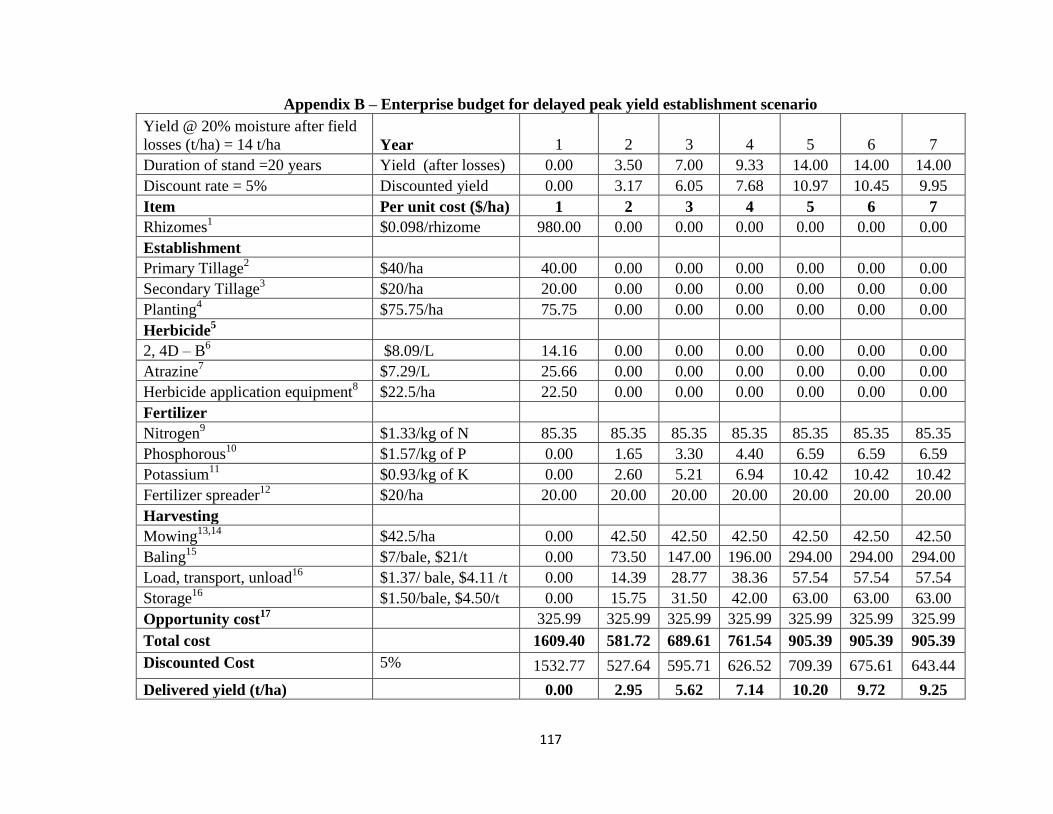
117

Appendix B – Enterprise budget for delayed peak yield establishment scenario

Yield @ 20% moisture after field

losses (t/ha) = 14 t/ha Year 1 2 3 4 5 6 7

Duration of stand =20 years Yield (after losses) 0.00 3.50 7.00 9.33 14.00 14.00 14.00

Discount rate = 5% Discounted yield 0.00 3.17 6.05 7.68 10.97 10.45 9.95

Item Per unit cost ($/ha) 1 2 3 4 5 6 7

Rhizomes1 $0.098/rhizome 980.00 0.00 0.00 0.00 0.00 0.00 0.00

Establishment

Primary Tillage2 $40/ha 40.00 0.00 0.00 0.00 0.00 0.00 0.00

Secondary Tillage3 $20/ha 20.00 0.00 0.00 0.00 0.00 0.00 0.00

Planting4 $75.75/ha 75.75 0.00 0.00 0.00 0.00 0.00 0.00

Herbicide5

2, 4D – B6 $8.09/L 14.16 0.00 0.00 0.00 0.00 0.00 0.00

Atrazine7 $7.29/L 25.66 0.00 0.00 0.00 0.00 0.00 0.00

Herbicide application equipment8 $22.5/ha 22.50 0.00 0.00 0.00 0.00 0.00 0.00

Fertilizer

Nitrogen9 $1.33/kg of N 85.35 85.35 85.35 85.35 85.35 85.35 85.35

Phosphorous10

$1.57/kg of P 0.00 1.65 3.30 4.40 6.59 6.59 6.59

Potassium11

$0.93/kg of K 0.00 2.60 5.21 6.94 10.42 10.42 10.42

Fertilizer spreader12

$20/ha 20.00 20.00 20.00 20.00 20.00 20.00 20.00

Harvesting

Mowing13,14

$42.5/ha 0.00 42.50 42.50 42.50 42.50 42.50 42.50

Baling15

$7/bale, $21/t 0.00 73.50 147.00 196.00 294.00 294.00 294.00

Load, transport, unload16

$1.37/ bale, $4.11 /t 0.00 14.39 28.77 38.36 57.54 57.54 57.54

Storage16

$1.50/bale, $4.50/t 0.00 15.75 31.50 42.00 63.00 63.00 63.00

Opportunity cost17

325.99 325.99 325.99 325.99 325.99 325.99 325.99

Total cost 1609.40 581.72 689.61 761.54 905.39 905.39 905.39

Discounted Cost 5% 1532.77 527.64 595.71 626.52 709.39 675.61 643.44

Delivered yield (t/ha) 0.00 2.95 5.62 7.14 10.20 9.72 9.25

118

Yield @ 20% moisture after field losses

(t/ha) = 14 t/ha Year 8 9 10 11 12 13 14

Duration of stand =20 years Yield (after losses) 14.00 14.00 14.00 14.00 14.00 14.00 14.00

Discount rate = 5% Discounted yield 9.48 9.02 8.59 8.19 7.80 7.42 7.07

Item Per unit cost ($/ha) 8 9 10 11 12 13 14

Rhizomes1 $0.098/rhizome 0.00 0.00 0.00 0.00 0.00 0.00 0.00

Establishment

Primary Tillage2 $40/ha 0.00 0.00 0.00 0.00 0.00 0.00 0.00

Secondary Tillage3 $20/ha 0.00 0.00 0.00 0.00 0.00 0.00 0.00

Planting4 $75.75/ha 0.00 0.00 0.00 0.00 0.00 0.00 0.00

Herbicide5

2, 4D – B6 $8.09/L 0.00 0.00 0.00 0.00 0.00 0.00 0.00

Atrazine7 $7.29/L 0.00 0.00 0.00 0.00 0.00 0.00 0.00

Herbicide application equipment8 $22.5/ha 0.00 0.00 0.00 0.00 0.00 0.00 0.00

Fertilizer

Nitrogen9 $1.33/kg of N 85.35 85.35 85.35 85.35 85.35 85.35 85.35

Phosphorous10

$1.57/kg of P 6.59 6.59 6.59 6.59 6.59 6.59 6.59

Potassium11

$0.93/kg of K 10.42 10.42 10.42 10.42 10.42 10.42 10.42

Fertilizer spreader12

$20/ha 20.00 20.00 20.00 20.00 20.00 20.00 20.00

Harvesting

Mowing13,14

$42.5/ha 42.50 42.50 42.50 42.50 42.50 42.50 42.50

Baling15

$7/bale, $21/t 294.00 294.00 294.00 294.00 294.00 294.00 294.00

Load, transport, unload16

$1.37/ bale, $4.11 /t 57.54 57.54 57.54 57.54 57.54 57.54 57.54

Storage16

$1.50/bale, $4.50/t 63.00 63.00 63.00 63.00 63.00 63.00 63.00

Opportunity cost17

325.99 325.99 325.99 325.99 325.99 325.99 325.99

Total cost 905.39 905.39 905.39 905.39 905.39 905.39 905.39

Discounted Cost 5% 612.80 583.62 555.83 529.36 504.15 480.15 457.28

Delivered yield (t/ha) 8.81 8.39 7.99 7.61 7.25 6.90 6.58

119

Yield @ 20% moisture after field

losses (t/ha) = 14 t/ha Year 15 16 17 18 19 20

Duration of stand =20 years Yield (after losses) 14.00 14.00 14.00 14.00 14.00 14.00

Discount rate = 5% Discounted yield 6.73 6.41 6.11 5.82 5.54 5.28

Item Per unit cost ($/ha) 15 16 17 18 19 20 Sum

Rhizomes1 $0.098/rhizome 0.00 0.00 0.00 0.00 0.00 0.00 980.00

Establishment

Primary Tillage2 $40/ha 0.00 0.00 0.00 0.00 0.00 0.00 40.00

Secondary Tillage3 $20/ha 0.00 0.00 0.00 0.00 0.00 0.00 20.00

Planting4 $75.75/ha 0.00 0.00 0.00 0.00 0.00 0.00 75.75

Herbicide5

2, 4D – B6 $8.09/L 0.00 0.00 0.00 0.00 0.00 0.00 14.16

Atrazine7 $7.29/L 0.00 0.00 0.00 0.00 0.00 0.00 25.66

Herbicide application equipment8 $22.5/ha 0.00 0.00 0.00 0.00 0.00 0.00 22.50

Fertilizer

Nitrogen9 $1.33/kg of N 85.35 85.35 85.35 85.35 85.35 85.35 1706.92

Phosphorous10

$1.57/kg of P 6.59 6.59 6.59 6.59 6.59 6.59 114.85

Potassium11

$0.93/kg of K 10.42 10.42 10.42 10.42 10.42 10.42 181.41

Fertilizer spreader12

$20/ha 20.00 20.00 20.00 20.00 20.00 20.00 400.00

Harvesting

Mowing13,14

$42.5/ha 42.50 42.50 42.50 42.50 42.50 42.50 807.50

Baling15

$7/bale, $21/t 294.00 294.00 294.00 294.00 294.00 294.00 5120.50

Load, transport, unload16

$1.37/ bale, $4.11 /t 57.54 57.54 57.54 57.54 57.54 57.54 1002.16

Storage16

$1.50/bale, $4.50/t 63.00 63.00 63.00 63.00 63.00 63.00 1097.25

Opportunity cost17

325.99 325.99 325.99 325.99 325.99 325.99 6519.80

Total cost 905.39 905.39 905.39 905.39 905.39 905.39 18,128.45

Discounted Cost 5% 435.51 414.77 395.02 376.21 358.29 341.23 11,355.29

Delivered yield (t/ha) 6.26 5.96 5.68 5.41 5.15 4.91 131.81

Breakeven farm gate price ($/t) 86.15

120

Appendix C- Enterprise budget for early establishment scenario

Yield @ 20% moisture after field

losses (t/ha) = 14 t/ha Year 2 3 4 5 6 7

Duration of stand =20 years Yield (after losses) 7.00 14.00 14.00 14.00 14.00 14.00

Discount rate = 5% Discounted yield 6.35 12.09 11.52 10.97 10.45 9.95

Item Per unit cost ($/ha) 2 3 4 5 6 7

Rhizomes1 $0.098/rhizome 0.00 0.00 0.00 0.00 0.00 0.00

Establishment

Primary Tillage2 $40/ha 0.00 0.00 0.00 0.00 0.00 0.00

Secondary Tillage3 $20/ha 0.00 0.00 0.00 0.00 0.00 0.00

Planting4 $75.75/ha 0.00 0.00 0.00 0.00 0.00 0.00

Herbicide5

2, 4D – B6 $8.09/L 0.00 0.00 0.00 0.00 0.00 0.00

Atrazine7 $7.29/L 0.00 0.00 0.00 0.00 0.00 0.00

Herbicide application equipment8 $22.5/ha 0.00 0.00 0.00 0.00 0.00 0.00

Fertilizer

Nitrogen9 $1.33/kg of N 85.35 85.35 85.35 85.35 85.35 85.35

Phosphorous10

$1.57/kg of P 3.30 6.59 6.59 6.59 6.59 6.59

Potassium11

$0.93/kg of K 5.21 10.42 10.42 10.42 10.42 10.42

Fertilizer spreader12

$20/ha 20.00 20.00 20.00 20.00 20.00 20.00

Harvesting

Mowing13,14

$42.5/ha 42.50 42.50 42.50 42.50 42.50 42.50

Baling15

$7/bale, $21/t 147.00 294.00 294.00 294.00 294.00 294.00

Load, transport, unload16

$1.37/ bale, $4.11 /t 28.77 57.54 57.54 57.54 57.54 57.54

Storage16

$1.50/bale, $4.50/t 31.50 63.00 63.00 63.00 63.00 63.00

Opportunity cost17

325.99 325.99 325.99 325.99 325.99 325.99

Total cost 689.61 905.39 905.39 905.39 905.39 905.39

Discounted Cost 5% 625.50 782.11 744.86 709.39 675.61 643.44

Delivered yield (t/ha) 5.90 11.25 10.71 10.20 9.72 9.25

121

Yield @ 20% moisture after field

losses (t/ha) = 14 t/ha Year 8 9 10 11 12

Duration of stand =20 years Yield (after losses) 14.00 14.00 14.00 14.00 14.00

Discount rate = 5% Discounted yield 9.48 9.02 8.59 8.19 7.80

Item Per unit cost ($/ha) 8 9 10 11 12 Sum

Rhizomes1 $0.098/rhizome 0.00 0.00 0.00 0.00 0.00 980.00

Establishment

Primary Tillage2 $40/ha 0.00 0.00 0.00 0.00 0.00 40.00

Secondary Tillage3 $20/ha 0.00 0.00 0.00 0.00 0.00 20.00

Planting4 $75.75/ha 0.00 0.00 0.00 0.00 0.00 75.75

Herbicide5

2, 4D – B6 $8.09/L 0.00 0.00 0.00 0.00 0.00 14.16

Atrazine7 $7.29/L 0.00 0.00 0.00 0.00 0.00 25.66

Herbicide application equipment8 $22.5/ha 0.00 0.00 0.00 0.00 0.00 22.50

Fertilizer

Nitrogen9 $1.33/kg of N 85.35 85.35 85.35 85.35 85.35 1706.92

Phosphorous10

$1.57/kg of P 6.59 6.59 6.59 6.59 6.59 69.24

Potassium11

$0.93/kg of K 10.42 10.42 10.42 10.42 10.42 109.37

Fertilizer spreader12

$20/ha 20.00 20.00 20.00 20.00 20.00 240.00

Harvesting

Mowing13,14

$42.5/ha 42.50 42.50 42.50 42.50 42.50 467.50

Baling15

$7/bale, $21/t 294.00 294.00 294.00 294.00 294.00 3087.00

Load, transport, unload16

$1.37/ bale, $4.11 /t 57.54 57.54 57.54 57.54 57.54 604.17

Storage16

$1.50/bale, $4.50/t 63.00 63.00 63.00 63.00 63.00 661.50

Opportunity cost17

325.99 325.99 325.99 325.99 325.99 3911.88

Total cost 905.39 905.39 905.39 905.39 905.39 11352.88

Discounted Cost 5% 612.80 583.62 555.83 529.36 504.15 8499.44

Delivered yield (t/ha) 8.81 8.39 7.99 7.61 7.25 97.09

Breakeven farm gate price ($/t) 80.22

122

Assumptions

1. Rhizomes are planted at a density of 1m2. Price per rhizome is the mean of the

price range found in the literature ($0.03 to $0.60).

2. Cost of primary tillage is determined using the cost of using a disc from

OMAFRA, 2009

3. Cost of secondary tillage is determined using the cost of harrowing from

OMAFRA 2009

4. Cost of planting rhizomes is estimated using the potato planter costs from Lazarus

et al., 2005

5. Herbicides are only applied in year 1

6. 2, 4D-B is applied at the rate of 1.75L/ha. Price is determines by taking a 5 year

average cost of 2,4D-B from McEwan, 2010

7. Atrazine is applied at the rate of 3.52L/ha. Price is determined by taking a 5 year

average cost of Atrazine from McEwan, 2010

8. Herbicides are applied using a pull type sprayer. Cost of application equipment is

taken from OMAFRA, 2009.

9. Nitrogen is applied at the rate of 64 kg N/ha. Application rate is the average rate

calculated from other field trials done (Table 3.2). Price is the 5 year average cost

of Nitrogen solution (UAN) from McEwan, 2010. Although UAN is a liquid it

provides a cost estimate for nitrogen.

10. Phosphorous is applied at the rate at which it is removed from the soil by the plant

which is 0.3 P kg/t DM. Price is the 5 year average cost of Triple Phosphate from

McEwan, 2010. Phosphorous is only applied year 2 onwards. Cost is yield

dependent.

11. Potassium is applied at the rate at which it is removed from the soil by the plants

which is 0.8K kg/t DM. Price is the 5 year average cost of Muriate of Potash

from McEwan, 2010. Potassium is only applied year 2 onwards. Cost is yield

dependent.

12. Cost is based on assumption of spreading dry fertilizer (OMAFRA, 2009)

13. Costs are based on hay production and maybe underestimated since the yields for

Miscanthus are 30 % - 40% higher (OMAFRA, 2006)

14. Raking may not be required if crop is sufficiently dry (OMAFRA, 2009)

15. Baling costs are based on the following assumptions: 1 square bale is 334 kg, 1

tonne has 3 bales, dimensions 1.15m x 1.15m x 1.15m. Density is 218

kg/m3(OMAFRA, 2006). Cost is yield dependent.

16. Cost is yield dependent.

17. Opportunity cost is calculated by taking the average of the net returns on corn,

soybean and wheat in Ontario (Table 3.3)