The Effect of Opportunity Costs on Candidate Supply

Guy Grossman and W. Walker Hanlon

January 21, 2009

1 Introduction

Small groups, such as the Ugandan farmer associations we investigate, are playing an in-creasingly vital role in creating growth in developing countries. The effectiveness of thesesmall groups often depends heavily on their ability to select an effective manager. Theproblem of selecting the most effective manager from within the organization can be brokendown into two parts. First, group members must decide whether to become candidatesfor the management position. Second, the group members must choose the manager fromamong the available set of candidates. This paper will offer a theory focusing on the firstof these problems: the self-selection of the candidate pool.

In deciding whether to become candidates for a management position, group membersmust consider several factors. First, if a member is chosen to be the manager, they willbe required to spend time and effort managing the organization’s affairs, which will entailsome opportunity cost. How large this opportunity cost is will depend on the income theycould receive from spending that time elsewhere, as well as on the amount of time and effortthey devote to managing the organization. In the case of the Ugandan farmer associations,member’s opportunity cost could depend on the size of their plot or on what they couldreceive outside the agricultural sector.

Second, as a member of the group, the manager will receive some benefits from theirown management. In addition to the direct benefits of holding office, both monetary andsocial, the manager may also benefit from the public good that they produce. The sizeof the benefits they receive will depend on their stake in the organization. These stakesmay take many forms. In a farmer’s cooperative, a member’s stake in the organizationdepends heavily on the size of the plot they farm. The larger (or more productive) the plotfarmed, the more they benefit from a negotiated increase in the sales price they receive, ora decrease in input prices, two of the primary tasks of the manager. When manager effortis non-contractible, these additional benefits may play an important role in motivatingmanager effort.

1

A group member’s candidacy decision may also depend on their probability of election ifthere are costs, either monetary or social, to being a candidate. In small groups, candidacycosts are likely to be quite small, so for simplicity we ignore this aspect of the decision.

We define candidate quality as the value of the public good that a candidate will deliverif they are chosen to be the manager. Thus, a candidate’s quality depends on a combinationof ability and effort. The small size of our groups means that members know each otherrelatively well, and so ability is well observed. However, once a candidate becomes themanager, it is often difficult for members to observe their day-to-day effort. Once thecandidate pool is determined, members will attempt to choose the candidate with thebest combination of ability and expected effort for the job. This suggests that factorsthat motivate potential candidates to exert more effort will play an important role in themanager selection process. In particular, the size of an manager’s stake in the public goodproduced by the organization may be an important factor in incentivizing effort, becausethe manager will benefit more from the public good they produce. In the context of thefarmer associations we study, a manager with a larger farm will benefit more from the publicgood they produce and so put more effort in as a manager. Since other group membersknow a candidates farm size, they will take the resulting incentive effects into account whenchoosing the manager.

The goal of this paper is to understand how opportunity costs impact the quality ofthe candidate pool in small groups, and through this channel, the ultimate quality of themanager. We present a simple model of candidate self-selection that allows us to con-duct comparative statics exercises. We simplify the voting behavior of members once thecandidate pool is formed, as this is not the focus of our attention.

This paper builds on the work of several previous projects looking at similar issues.Caselli & Morelli (2004) was perhaps the first paper to focus attention on how the supplyof candidates affected the quality of the ultimate office holders. They suggest that officeholders differ in two dimensions: competence and honesty. In their model, more competentcitizens have higher opportunity costs of holding office, while more honest citizens receivefewer rewards from holding office because they are less willing to use their position forpersonal gain. A main result of this paper is that, due to opportunity costs, more competentpoliticians may decide not to run for office. Similarly, more honest politicians may decidenot to run because they will receive smaller benefits from office. Our model will build onthese ideas.

One respect in which our model differs from Caselli & Morelli (2004) is that they areconcerned with elections in large groups where citizens have imperfect information aboutcandidates, while we focus on small groups where group members are fairly well informed

2

about the abilities of other members. In this scenario, the role of voter error resulting fromimperfect information is reduced, while the importance of the candidate pool is magnified.Thus, this is arguably a more compelling area in which to study the selection of the can-didate pool. Another difference between the large and small group cases is that when thepopulation is large, each individual candidate’s stake in the public good is relatively small,while in small groups, each candidate’s relative stake in the public good is much larger.Thus, the incentive effects of a candidate having a larger stake in the group will be muchstronger for small groups.

Perhaps the most similar research to our work is Messner & Polborn (2004). Theyfocus on how selection of the candidate pool affects outcomes in a small group situation,where candidate’s actual ability is well known. This allows them to abstract from thevoting problem and focus attention on selection of the candidate pool. They follow Caselli& Morelli (2004) in exploring the role of opportunity costs in affecting the quality of thecandidate pool, though in Messner and Polborn’s model there is only one office holder,rather than many offices to be filled, as in Caselli and Morelli. We will follow an approachthat is similar to Messner & Polborn (2004) in many respects.

Where we differ from these previous studies is in our treatment of the opportunity costsfaced by potential candidates. Both of the previous studies assume that higher qualitycitizens have, at least on average, higher opportunity costs, but they give little considerationto what these costs actually represent. Our contribution, in essence, is to ‘unpack’ thesecosts. We suggest that in addition to being correlated with ability, some opportunity costsmay also be correlated with the gains potential candidates receive from the public goodproduced by the office holder. When office holders have to determine how much effort toput into their post, this becomes an important point that may significantly change thelessons drawn from these models.

Our theoretical results suggest that the characteristics of the opportunity costs faced bygroup members play a key role in determining outcomes. Pure opportunity costs that haveno relationship the the public good are found to reduce the quality of the candidate pooland the manager quality. In terms of our farmer associations, off-farm income opportunitiescreate opportunity costs of this kind. This result matches previous work. However, we alsofind that opportunity costs that are related to how much an individual benefits from thepublic good may increase the quality of the candidate pool and the value of the public goodproduced by the manager. In our example such opportunity costs may correspond to farmsize or productivity. This result contrasts with previous work and suggests that nuance isrequired in considering the effect of opportunity costs on the candidate pool and managerquality.

3

2 Model

We begin this section by introducing the basic framework of our model. Each individual’sopportunity cost of becoming the manager depends on their endowments. We divide theseendowments based on whether they do or do not affect how individuals benefit from thepublic good. In keeping with our interest in farmer associations, we call these farm andoff-farm income opportunities, respectively. We then describe how variation in these endow-ments affects the amount of effort that an individual will put into producing public goodsfor their group if they are elected manager. Next, we describe how individual’s endowmentswill affect their candidacy decision given their optimal effort choice. Individual’s candidacydecision is given as a function of the next best available candidate. Thus, we remain agnos-tic about the particular characteristics of the group members, an assumption that we willrelax in Section 3.

A group is composed of N members indexed by i ∈ [1, N ]. Group members differ intheir ability, Ai, in their farm income opportunities, Si, which may represent things likefarm size or productivity, and in their off-farm income opportunities, Ki. It is likely thatboth Si and Ki will be correlated with Ai. Each group will eventually choose at most onemanager, who will divide her time between management, which produces public goods forthe group, work on her own farm, and off-farm work. Other group members divide theirtime between work on their own farm and off-farm work. Each individual is endowed withone unit of available labor. The manager will allocate some portion e ∈ [0, 1] of her time toproducing public goods for the group, and the remainder to work on her own farm or onoff-farm work. All other individuals will allocate all of their time to work on their farm oroff-farm work, i.e. for individuals who are not the manager, e = 0.

The public good produced if individual j is the manager is given by the continuousfunction M(Aj , ej). Public goods production is increasing in both the manager’s abilityand the amount of effort they devote to public goods production.

∂M

∂Aj> 0 and

∂M

∂ej> 0

An individual i’s payoff from working on their own farm is given by the continuousfunction F (Si, (1 − ei),Mj) where Mj represents the public good produced by manager jand (1 − ei) represents the amount of time not devoted to group management 1. Notethat whenever i 6= j, ei = 0. Farm income is increasing in an individual’s farm incomeopportunities. Farm income is weakly decreasing in the effort that an individual devotes to

1Implicit in both the F() and G() functions is the assumption that all individuals face the same input

and output prices. Since these are generally negotiated by the manager for the group, this assumption seems

quite reasonable.

4

management, ei, (holding the value of the public good constant) which equals zero for allindividuals except the manager. Farm income is increasing in the value of the public goodproduced by the manager.

∂F

∂Si> 0 ,

∂F

∂ei≤ 0 ,

∂F

∂Mj> 0

An individual i’s payoff from off-farm work is given by the continuous function G(Ki, (1−ei)). Off-farm production is increasing in an individual’s ability, their available human andphysical capital, and weakly decreasing in the amount of effort they devote to managingthe group’s activities.

∂G

∂Ki> 0 ,

∂G

∂ei≤ 0

Individually, farm and off-farm incomes are each weakly decreasing in the amount ofeffort devoted to management because when more effort is devoted to management, lesseffort is available to farm and off-farm work. The reason that farm production is only weaklydecreasing in ei is because individuals will allocate the time not devoted to managementoptimally between on and off-farm work. The only assumption we place on how this residualtime (1− ei) is allocated is that the amount of effort put into either farm or non-farm workwill never decrease in the amount of residual time. In other words, if the manager decidesto put less time into management activities, this will never result in a decrease in the timeput into either farm or off-farm work. At the least, the amount of time put into either farmor off-farm work will remain constant; generally it will increase. The partial derivate of thesum of farm and off-farm returns with respect to the effort devoted to management will bestrictly decreasing, since effort devoted to management must come out of either one or theother of these activities.

∂(F +G)∂ei

< 0

Each of the three activities, management, on-farm work, and off-farm work, suffer fromdiminishing returns in the amount of effort devoted to that activity.

∂2M

∂e2i< 0 ,

∂2F

∂e2i≤ 0 ,

∂2G

∂e2i≤ 0

There are three other key assumptions in our model. The first deals with the comple-mentarity between capital (or opportunity) and labor.

Assumption 1 The marginal benefit of putting time into farm work is increasing in S,while the marginal benefit of putting time into off-farm work are increasing in K.

∂2F

∂ei∂Si≤ 0 ,

∂2G

∂ei∂Ki≤ 0

5

The second key assumption stems from a crucial difference between an individual’sincome from farm and off-farm work. If an individual decides to put less time into farmwork, they are generally able to hire someone to do the same work and can still enjoycapital’s share of the benefits from this work. However, if an individual decides to reducethe time they put into off-farm labor, they lose all of the income they could have madefrom that activity. This suggests the following relationship between the marginal benefitof putting time into the off-farm sector relative to the marginal benefit from putting timeinto the farm sector.

Assumption 2 A small increase in the amount of effort devoted to management activityreduces the marginal benefit of an additional unit of farm income opportunity more than itreduces the marginal benefit of an equal sized unit of additional off-farm income opportunity.∣∣∣∣∣ ∂2F

∂ei∂Si

∣∣∣∣∣ <∣∣∣∣∣ ∂2G

∂ei∂Ki

∣∣∣∣∣ for any Mj (1)

There is also complementarity between the public good and farm income opportunities.When the public good produced by the manager is better, the return to an additional unitof farm income opportunity is increased. Conversely, when an individual has more farmincome opportunity, their marginal benefit from an increase in the value of the public goodincreases. In practical terms, when the manager is able to negotiate a better price for sellingfarm output, this increases the marginal benefit of additional farm production.

Assumption 3 The cross-partial derivative of farm income on the public good and farmsize is positive.

∂2F

∂Si∂M> 0

These will be important assumptions in determining how an individual’s endowmentsaffect the amount of effort they are willing to devote to management, the topic of the nextsection.

2.1 Manager’s choice of effort level

The manager, which we denote with the subscript m, will choose effort in order to maximizethe sum of her returns from all sources. In other words, she will solve the following problem.

maxemF (Sm, (1− em),M(Am, em)) +G(Km, (1− em))

The manager is optimizing a continuous function on the compact set em ∈ [0, 1], soan optimal effort level will exist. The manager’s optimal effort level equates her marginalproduct from management with that from farm and off-farm activities.

6

∂F

∂M

∂M

∂em= −

[∂F

∂em+

∂G

∂em

](2)

The solution to this problem will be unique when the following condition, which ensuresthe convexity of the objective function, holds.

∂2F

∂M∂em

∂M

∂em+∂F

∂M

∂2M

∂e2m< −

[∂2F

∂e2m+∂2G

∂e2m

](3)

This condition will fail only if the left hand term is positive and large, i.e. only if themarginal return to management effort em is increasing despite the decreasing returns tomanagement effort in producing the public good. Note that the second term is negativebecause ∂2M/∂e2m < 0 while the right hand side is positive. The above condition failsonly if the marginal product of management is strongly decreasing in the amount of effortput into on-farm labor. However, we expect exactly the opposite – the marginal returnto management should be increasing in the amount of effort put into on-farm labor (ordecreasing in em). Thus, we can safely impose the following assumption, which ensuresthat the manager’s optimal effort level is unique.

Assumption 4 An individual’s marginal benefit from the public good created by the man-ager is increasing in the amount of effort put into farm labor, which is weakly decreasing inthe amount of effort devoted to management activities, ei.

∂2F

∂M∂ei≤ 0

Hereafter, we denote the manager’s optimal effort level as e∗i if individual i is the man-ager. Next, we want to explore how this optimal effort level is affected by changes in themanager’s farm and off-farm income opportunities.

Proposition 1 Under the assumptions we have given, the manager’s optimal effort level,e∗, is decreasing in their off-farm income opportunities.

∂e∗

∂Km< 0

Proof: Because the marginal benefit of the manager’s effort devoted to off-farm work is increasing in Km, we know that an increase in Km will lead toan increase in the right hand side of Equation 2. Thus, either the left handside of 2 must increase, or the right hand side must decrease, to compensate.The left hand side of Equation 2 is decreasing in e∗, while the right handside is increasing in e∗, so e∗ must decrease in response to the increase inKm. QED

7

The effect of increased Sm on the manager’s effort decision is slightly more complicated.Increased farm income opportunities increase the benefits of putting effort into farm work,but also increase the benefits of management effort. In Equation 2, an increase in Sm causesan increase in both the left hand side, which will tend to increase e∗, and increase in theright hand side, which will tend to decrease e∗. Thus, whether an increase in Sm increasesor decreases the manager’s effort level is ambiguous.

One thing we can say is that even if one additional unit of Sm causes a decrease in themanager’s effort level, this decrease will always be smaller than the decrease resulting froman equivalent increase in Km. This follows from Assumption 1. This point is made moreformally in the following theorem.

Proposition 2 When Assumption 1 holds, the effect of the manager’s farm size Sm ontheir optimal effort level is ambiguous. However, even if the manager’s optimal effort levelis decreasing in their farm size, this decrease will never be as large as the decrease resultingform an increase in their off-farm income potential.

de∗

dKm<

de∗

dSm(4)

Proof: Rewriting Equation 2, we can see that the manager’s optimal effortlevel e∗ solves the following.

H ≡ ∂F

∂M

∂M

∂em+

∂F

∂em+

∂G

∂em= 0

From Equation 3, we know that dH/dem < 0. Next, we take the derivativeof the function H with respect to Km, and then with respect to Sm.

dH

dKm=

∂2G

∂Km∂em≤ 0

dH

dSm=

∂2F

∂Sm∂em

∂M

∂em+

∂2F

∂Km∂em

It follows from Assumption 1 that,

dH

dKm<

dH

dSm

In other words, a small change in Km reduces H at a more rapid rate thanan equivalent small change in Sm. Since H is decreasing in em, this impliesthat there will have be a larger decrease in e∗ to offset an increase in Km

than will be required to offset an equivalent decrease in Sm. QED

8

In this section, we have shown that an increase in the manager’s off-farm income op-portunities decreases the effort she puts into management. We have also shown that anincrease in the manager’s farm income opportunities may increase or decrease the effortshe puts into management, but that it will never cause as large a reduction in managementeffort as an equivalent increase in off-farm income opportunities. These results have directimplications for the value of the public good produced by the manager, which we describebelow.

Corollary 1 The value of the public good created by a manager is decreasing in their off-farm income opportunities and may be increasing or decreasing in their farm income op-portunities. The value of the public good will never be decreasing as rapidly in their farmincome opportunities as it is in their off-farm income opportunities.

dM(Ai, ei)dKi

< 0 anddM(Ai, ei)

dKi<dM(Ai, ei)

dSi

These relationships will be important to group member’s candidacy decision, the topicof our next section.

2.2 Group member’s candidacy choice

In this section we explore how an individual’s probability of candidacy is affected by theirendowments taking as given the existence of some best alternative manager. We leave thequestion of how the best alternative manager is identified out of the set of members of thegroup, and how this affects an individual’s candidacy decision, for later sections.

When there are no costs to being a candidate, group members will choose to be acandidate only if their payoff from being the manager exceeds their payoff from not becomingthe manager. If an individual chooses not to become a candidate, then their payoff willdepend on the public good delivered by the person who does become the manager. DefineJi to be the difference between individual i’s payoff as the manager and their payoff as aregular group member, as below, where individual j is the best alternative candidate formanager. The exogenously given remuneration for the manager is R.

Ji ≡ F (Si, (1− ei),M(Ai, ei)) +G(Ki, (1− ei))− F (Si, 1,M(Aj , ej))−G(Ki, 1) +R (5)

A group member will choose to become a candidate only if Ji ≥ 0. Of course, whetherthis holds depends on the set of other potential candidates. Once groups have been formed,it is easy for an individual to simply look across all other group members and decide whothe best alternative manager is. In this section, we are interested in how an individual’s

9

endowment affects their ex ante probability of choosing to be a candidate. The ex anteprobability that some individual i will choose to be a manager is given below.

Pr [F (Si, (1− ei),M(Ai, ei)) +G(Ki, (1− ei))− F (Si, 1,M(Aj , ej))−G(Ki, 1) +R ≥ 0](6)

2.2.1 Effect of off-farm income opportunities

How is a member’s probability of candidacy affected by her endowments? First we considerhow off-farm income opportunities affect an individual’s candidacy decision. Our result isdescribed in the following proposition.

Proposition 3 An individual’s probability of candidacy is decreasing in her off-farm in-come opportunities.

dJidKi

< 0

10

Proof: The effect of a small increase in Ki on Ji is described below, wherefor notational simplicity the superscript ‘M’ is used to denote that she isthe manager (and ei = e∗i ) and ‘I’ denotes that she is not the manager (andei = 0).

dJidKi

=∂FM

∂e∗i

de∗idKi

+∂FM

∂Mi

∂MM

∂e∗i

de∗idKi

+∂GM

∂e∗i

de∗idKi

+∂GM

∂Ki− ∂GI

∂Ki

Note that at ei = e∗i implies,

∂FM

∂e∗i+∂FM

∂Mi

∂MM

∂e∗i+∂GM

∂e∗i= 0

So our expression simplifies to the following.

dJidKi

=∂G(Ki, (1− e∗i ))

∂Ki− ∂G(Ki, 1)

∂Ki

We have assumed that Ki and ei are complements, so we can see that anincrease in Ki will weakly increase the individual’s return more when theyare not the manager. The inequality will become strict whenever e∗i > 0.

∂G(Ki, (1− e∗i ))∂K

≤ ∂G(Ki, 1)∂K

with strict inequality whenever e∗i > 0

We can now see that an increase in an individual’s off-farm income oppor-tunities reduces the probability that they will choose to be a candidate formanager.

2.2.2 Effect of farm income opportunities

Understanding the effect of an increase in individual’s farm income opportunities on theirprobability of candidacy is not as straightforward as the previous exercise. We begin withthe effect of a small increase in Si on Ji, given below, where again we use the superscripts‘M’ and ‘I’ to signify payoffs when the individual is and is not the manager, respectively.

dJidSi

=∂FM

∂e∗i

de∗idSi

+∂FM

∂Mi

∂MM

∂e∗i

de∗idSi

+∂FM

∂Si+∂GM

∂e∗i

de∗idSi− ∂F I

∂Si

As before, we can use the definition of e∗ to simplify.

dJidSi

=∂F (Si, (1− e∗i ),M(Ai, e∗i , V ))

∂Si−∂F (Si, 1,M(Aj , e∗j , V ))

∂Si

An individual’s marginal return to their farm income opportunities is increasing in theamount of effort devoted to farm work. Alone, this effect would suggest that an individual’s

11

probability of candidacy is decreasing in their farm income opportunities. However, this isnot the only effect working in this case. An individual’s marginal return to farm incomeopportunities is also affected by the value of the public good. If an individual is a betterchoice for manager than their next best alternative, so that M(Ai, e∗i , V ) > M(Aj , e∗j , V ),then their probability of candidacy may be increasing in their farm income opportunities.This is because group members with larger farms benefit more from the extra public goodsthat they are able to produce if they are a better manager than the alternative.

Overall, the effect of farm income opportunities on an individual’s probability of candi-dacy is ambiguous. One thing we can say is that an increase in farm income possibilities willnever reduce and individual’s probability of candidacy as much as an equivalent increase inoff-farm income opportunities. This point is made formally below.

Proposition 4 The effect of an increase in an individual’s farm income opportunities onthe probability of candidacy may be positive or negative. However, when Assumption 1holds, an individual’s probability of candidacy will always decrease more from an increasein their off-farm income opportunities than it will from an equivalent increase in their farmincome opportunities as long as the public good produced by the individual is more valuablethan the public good produced by the next best manager.

dJidKi

<dJidSi

when M(Ai, e∗i ) > M(Aj , e∗j )

12

Proof: We begin by expanding the function J, using the simplifications fromthe previous two proofs.

dJidKi− dJidSi

=∂G(Ki, (1− e∗i ))

∂Ki− ∂G(Ki, 1)

∂Ki− ∂F (Si, (1− e∗i ),Mi)

∂Si+∂F (Si, 1,Mj)

∂Si

=∂G(Ki, (1− e∗i ))

∂Ki− ∂G(Ki, 1)

∂Ki− ∂F (Si, (1− e∗i ),Mi)

∂Si

+∂F (Si, 1,Mi)

∂Si− ∂F (Si, 1,Mi)

∂Si+∂F (Si, 1,Mj)

∂Si

=∫ e∗i

0

(∂2G(Ki, (1− ei))

∂Ki∂ei− ∂2F (Si, (1− ei),Mi)

∂Si∂ei

)dei −∫ Mi

Mj

∂2F (Si, (1− ei),M)∂Si∂M

dM < 0

That the first integral is negative follows from Assumption 2, which statesthat an increase in the amount of effort devoted to management decreases themarginal benefit from additional off-farm income opportunities more thanthe marginal benefit from farm income opportunities. That the value underthe second integral is positive follows from Mi > Mj and Assumption 3.

2.3 Voting and group outcomes

In this section, we consider how the behaviors we have described translate into an actualcandidate pool and manager choice. Our approach will be to solve backwards. We firstconsider member’s voting behavior given an available pool of candidates and then turnto how the actual pool of candidates is determined given that everyone knows the votingoutcome once the candidate pool is formed. In the following section, we consider howexogenous factors will affect the quality of the candidate pool and the manager that thegroup selects.

Every group member’s ability, farm, and off-farm income opportunities, are perfectlyobserved by all other members of their small group. Also, the voting incentives of all groupmembers are perfectly aligned; they all want the highest value public good possible. Closelyaligned incentives and the availability of ample information about other members are keyfeatures of the small group situation we are concerned with.

Once the candidate pool is determined, members will be able to deduce the value ofthe public good that each candidate will produce. They simply pick the candidate who

13

will deliver the highest value public good 2. One implication of this voting behavior is thatthere is no chance that a less qualified candidate will be chosen over a more qualified onedue to voter error or lack of information.

Having specified member’s voting behavior, we can now consider how the candidatepool is formed. To do this, we order all group members in an increasing line according tothe value of the public good that they will produce given their endowments and adjust theindividual indexes (i) accordingly. So individual i=1 will deliver the lowest value publicgood out of all group members, and individual i=N will deliver the highest value publicgood.

Next, note that, as a result of the voting system, an individual’s candidacy decision doesnot depend on the candidacy decisions of anyone ordered above them. To see why, supposeindividual i is trying to decide whether to be a candidate. If some individual j > i decidesto be a candidate, then individual i is indifferent between being a candidate or not, sincethey will never be elected. If no individual ordered above i decides to be a candidate, thenindividual i will face a relevant candidacy choice. So, if i makes their candidacy decisionassuming that none of the individuals ordered above them will run, then they will alwaysreach their optimal solution. Thus, each individual’s candidacy decision is made as if theyknow that none of the individual’s above them will join the candidate pool.

We can now construct an algorithm that obtains the candidate pool given a set of groupmembers. We begin with individual i=1 and work our way up. The member who willproduce the lowest value public good (i=1) will face the following decision, where the thevalue of the public good produced if no one decides to be a candidate for manager is zero.

Run if F (S1, (1− e∗1),M(A1, e∗1)) +G(K1, (1− e∗1)) +R ≥ F (S1, 1, 0) +G(K1, 1)

Based on this, individual 1 either chooses to run or not to run. Given their decision,individual 2 will behave as follows.

If individual 1 decided to run,

Run if F (S2, (1− e∗2),M(A2, e∗2)) +G(K2, (1− e∗2)) +R ≥ F (S2, 1,M(A1, e

∗1)) +G(K2, 1)

If individual 1 decided not to run,

Run if F (S2, (1− e∗2),M(A2, e∗2)) +G(K2, (1− e∗2)) +R ≥ F (S1, 1, 0) +G(K1, 1)

2If two candidate’s endowments result in them delivering a public good of the same value, then voter’s

randomize between them, though because we are dealing with continuous distributions of ability, farm, and

off-farm income opportunities, such a result is unlikely, so we do not consider it further.

14

For the i’th individual, if we denote the next best individual as j, then they will behaveas follows.

Run if F (Si, (1− e∗i ),M(Ai, e∗i )) +G(Ki, (1− e∗i )) +R ≥ F (Si, 1,M(Aj , e∗j )) +G(Ki, 1)

Applying this algorithm to any group of individuals, we are able to construct the can-didate pool. The manager will then be the person in the candidate pool who will deliverthe highest valued public good.

What will the manager and candidate pool generated using this process look like? Thisis a hard question to answer without having a concrete set of group members. The candidacydecision depends crucially on the spacing between the values of the public goods generatedby different people. Variation in the spacing of these values depends on both the distributionof endowments and the number of group members. In the next section, we select a setof group members from a hypothetical endowment distribution and, after applying thealgorithm we have just outlined, study the resulting candidate pool and manager quality.

3 Simulated results

In the previous section, we described how, given a set of group members, each with aparticular set of endowments, we can determine the candidate pool and the manager. Inthis section, we take a step back and suppose that the group members have not yet beenchosen. Instead, we are faced with distributions of potential abilities, off-farm incomeopportunities, and farm sizes. We randomly draw the characteristics of N individuals fromthese distributions and then determine the candidate pool and manager choice that resultsfrom this group of individuals. Repeating the process many times, we can identify patternsin how the endowment distributions and other model parameters affect the candidate pooland the quality of the manager.

To begin this process, we need to assume particular functional forms. For simplicitywe will use the following functions, which have been derived from simple Cobb-Douglasproduction functions for farm, off-farm, and public good production. The details of thisderivation are described in Appendix A. Built into the functional forms for the F and G

functions is an optimal allocation of the effort not devoted to management between farmand off-farm work.

F =S(1− e)1−αM1/α

(K + SM1/α)1−αG =

K(1− e)1−α

(K + SM1/α)1−αM = ααAβi e

1−βi

In order to be sure that a unique optimal solution to each individual’s choice of effortin the event they are the manager (i.e., to satisfy Assumption 4), we require α+ β ≥ 0. Tosee why this conditions is necessary, refer to Appendix B.

15

We use simple uniform distributions for ability, farm, and off-farm income opportuni-ties. Each individual’s ability is chosen from a continuous uniform (0,1) distribution. Anindividual’s farm and off-farm income opportunities depend on both ability and on otherfactors.

S = bs + csA+ (1− cs)εsK = bk + ckA+ (1− ck)εk

Where A ∼ unif(0, 1) and the independent shocks on farm size and off-farm incomeopportunities depend on εs ∼ unif(0, 1) and εk ∼ unif(0, 1). The parameters bs ≥ 0 andbk ≥ 0 shift the distributions for S and K while the parameters cs ∈ (0, 1) and ck ∈ (0, 1)give the correlation between A and S and A and K, respectively.

The bk parameter represents exogenous factors that affect the (ex ante) off-farm incomeopportunities for all group members. Possible real-world parallels for this parameter includeproximity to a city, commercial center, or important trade route. Similarly, bs representsexogenous factors that affect ex ante farm income opportunities. This may represent theavailability and fertility of land in the area, fluctuations in world agricultural prices, etc.

Once the characteristics of each of the individuals in a group have been drawn fromthe given distributions, we solve the model as described in the previous sections. In orderto get some idea of what we can expect from each set of parameter values, we repeat theprocedure one hundred times for each set of parameters values and consider the averageresults.

Our first set of simulation results, in Figure 1, describe how the outcomes are affectedby increases in the bk parameter.3 The results in the top left figure suggest that larger bkparameters result in, on average, a manager that delivers a less valuable public good. Thetop right figure indicates that a reduction in manager effort is the key factor in reducingmanager quality. The rank of the manager, which orders each group member by the valueof the public good they would deliver as a manager (with 10 being the best), is not stronglyaffected by increases in off-farm income opportunities. Neither is the average ability of themanager. Thus, a fall in manager effort appears to be the crucial channel relating off-farmincome opportunities and manager quality.

3These results were calculated with parameters α = .6, β = .4, bs = 0, and ck = cs = .5. Appendix C

shows that similar results are obtained for a variety of other parameter values.

16

Figure 1: Effects of Off-farm Income Opportunities on the Manager

Average Manager Quality Average Manager Effort

Average Manager Rank Average Manager Ability

17

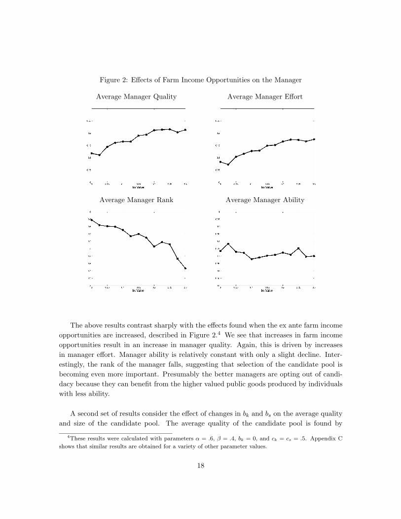
Figure 2: Effects of Farm Income Opportunities on the Manager

Average Manager Quality Average Manager Effort

Average Manager Rank Average Manager Ability

The above results contrast sharply with the effects found when the ex ante farm incomeopportunities are increased, described in Figure 2.4 We see that increases in farm incomeopportunities result in an increase in manager quality. Again, this is driven by increasesin manager effort. Manager ability is relatively constant with only a slight decline. Inter-estingly, the rank of the manager falls, suggesting that selection of the candidate pool isbecoming even more important. Presumably the better managers are opting out of candi-dacy because they can benefit from the higher valued public goods produced by individualswith less ability.

A second set of results consider the effect of changes in bk and bs on the average qualityand size of the candidate pool. The average quality of the candidate pool is found by

4These results were calculated with parameters α = .6, β = .4, bk = 0, and ck = cs = .5. Appendix C

shows that similar results are obtained for a variety of other parameter values.

18

Figure 3: Effects on the Candidate Pool

Effects of Off-Farm Income OpportunitiesAverage Pool Quality Average Pool Size

Effects of Farm Income OpportunitiesAverage Pool Quality Average Pool Size

averaging over the values of the public good that each candidate would produce if theywere the manager. As Figure 3 shows, these results largely parallel the manager results.Increases in off-farm income opportunities decrease the average quality of the candidatepool, though there is very little effect on the size of the candidate pool. Increases in on-farm income opportunities increase the quality of the candidate pool but also have littleeffect on the pool size. These results are important in the event that voters may make amistake and elect a candidate other than the most qualified.

19

4 Empirical specifications- WORK IN PROGRESS

Testing this model can be approached either through testing individual or group outcomes.These correspond to the individual results presented in Section 2 and Section 3 respectively.We begin by discussing approaches to testing the individual-level predictions of the model.

4.1 Empirical specifications for individual-level tests

The model has predictions for how an individual’s effort and the value of the public goodthey produce, if they are the manager, are affected by changes in their farm and off-farmincome opportunities. However, because only one individual in each group becomes themanager, it is very difficult to test these predictions. It will be more fruitful to considerthe model’s predictions regarding each individual’s probability of candidacy, as describedby Propositions 3 and 4. These propositions suggest that an individual’s probability ofcandidacy will be decreasing in their off-farm income. Also, while their probability ofcandidacy may be increasing or decreasing in their on-farm income, an increase in on-farmincome will never decrease their probability of candidacy as much as an increase in off-farmincome.

Suppose we begin with the following basic empirical specification, where Cij is an indi-cator function for whether individual i in group j chooses to become a candidate, Kij is theindividual’s off-farm income opportunities, Sij is the individual’s farm income opportuni-ties, Dj represents group fixed effects, and Xij represents a vector of the individual’s otherrelevant characteristics.

Cij = α+ βkKij + βsSij +Xijλ+Dj + εij (7)

The model makes the following two predictions.

βk < 0 βk < βs

Implementing an empirical specification of this type requires overcoming two differentbut related hurdles. First, we must identify the relevant variables in the data. We canidentify an individual’s candidacy choice in two ways. The manager must have choses tobe a candidate, so that is one sure indicator. We can also derive a second indicator byasking group members whether they considered being a candidate for manager. Otherindicators may also be possible. Data on individual’s farm and off-farm income streamswill be collected as part of our data gathering process. We will also collect individual data

20

on education, experience, etc. These data will be important in addressing omitted variablebias issues.

The classic problem with empirical work of this kind arises from omitted variable bias.If either of our explanatory variables of interest, Kij and Sij are correlated with the errorterm, then our estimates of βk and βs may be biased. Since both of these variables arelikely to be correlated with individual ability, this is a very real concern. Three approachesto this problem suggest themselves.

One approach to dealing with the omitted variable bias arising through the positivecorrelation between both farm and off-farm income and ability is to figure the direction ofthe bias. We expect that higher ability will make an individual more likely to be a candidatefor office. Ability should also be positively correlated with both farm and off-farm income.Thus, the coefficients on both farm and off-farm income should be biased upwards. Underthese assumptions, a finding that the estimated coefficient β̃k is significantly less than zerois sufficient evidence to confirm the first of our two predictions. Furthermore, we expectthat the correlation between off-farm income potential and ability should be larger thanthe correlation for farm income potential because farm income potential is also likely to beaffected by exogenous factors such as inheritance. Under this assumption, our estimate ofβk should have a larger upward bias than our estimate of βs, and β̃k < β̃s significant issufficient evidence that βk < βs.

If our first approach is not satisfied, or not sufficiently convincing, a second approachis to attempt to sufficiently control for ability. ‘Moving’ ability out of the error term bycontrolling for factors such as education and experience should reduce any omitted variablebias suffered by our coefficient estimates. Considering the direction of the remaining bias,as in the previous approach, can then be applied. This approach differs from the previousone only in that our parameter estimates should be more precise.

If the previous two approaches are not sufficiently convincing, an alternative is to lookfor instruments for Kij and Sij .

4.2 Empirical specifications for group-level tests

Results from Section 3 can be tested using group-level results for the chosen manager. Oursimulations suggest that manager effort is generally decreasing in a group’s ex ante off-farm income opportunities, and generally increasing in ex ante farm income opportunities.Similarly, manager quality is decreasing in a group’s ex ante off-farm income opportunities,and generally increasing in ex ante farm income opportunities.

21

Suppose we start with the following empirical specifications, where ej is the effort ofthe manager of group j, Mj is the quality of the public good produced by the manager ofgroup j, Sj and Kj represent average farm and off-farm income opportunities in the group,respectively, and Xj contains a vector of other group characteristics that affect managereffort or public good quality.

ej = α+ βkKj + βsSj +Xjλ+ εej (8)

Mj = a+ bkKj + bsSj +Xjγ + εMj (9)

The model makes the following predictions.

βk < 0 βs > 0

bk < 0 bs > 0

We may also want to test a second, weaker set of predictions.

βk < βs bk < bs

Our group-level tests confront difficulties that are similar to those addressed in theindividual-level tests. As before, we must identify variables that can act as proxies forsome of our unobserved variables of interest. We collect indicators of manager effort fromour manager questionnaire, as well as other indicators of manager effort. The value of thepublic good can be found by considering the input costs and output sales prices negotiatedby managers. On and off-farm income opportunity data come from individual incomereports. Importantly, we hope to gather exogenous group-specific data that can be usedas instruments for Kj and Sj . These data will likely relate to geographic factors such asproximity of nearest town, commercial center, or road, growing conditions, crop type, etc.

Omitted variable bias will occur in this specification if our variables of interest, Kj

and Sj are correlated with the error terms. This may occur if there are other factors thatare related to both a group’s farm and off-farm income opportunities and the manager’seffort of the value of the public good they produce. Such factors may come in a variety offorms.[More]

A Functional Form Derivation and Verification

We assume the following functional forms, where c is a constant that is equal to αα (forreasons that we will see later).

22

M = cAβe1−β

F = Sα[(1− e)γ]1−αM

G = Kα[(1− e)(1− γ)]1−α

First, we allow individuals to optimize their allocation of effort between farm and off-farm work.

maxγ

Sα[(1− e)γ]1−αM +Kα[(1− e)(1− γ)]1−α

The first order condition is:

(1− α)Sα(1− e)1−αγ−αM − (1− α)Kα(1− e)1−α(1− γ)−α = 0

Solving gives,

γ =SM1/α

K + SM1/α

The second order condition confirms that this is indeed an optimal solution.

−α(1− α)Sα(1− e)1−αγ−α−1 − α(1− α)Kα(1− e)1−α(1− γ)−α−1 < 0

Now our equations for F an G are:

F =S(1− e)1−αM1/α

(K + SM1/α)1−α

G =K(1− e)1−α

(K + SM1/α)1−α

Now we need to confirm that these equations conform to the assumptions we have made.We consider each assumption in the order in which it is introduced in the main text of thispaper. To begin, we show that the value of the public good is increasing in an individual’sability and in the amount of effort the manager puts into their job.

∂M

∂A= cβAβ−1e1−β > 0

∂M

∂e= c(1− β)Aβe−β > 0

23

Next, we want to show that, holding all else constant, the value of farm income isincreasing in farm size, decreasing in effort devoted to management, and increasing in thevalue of the public good.

∂F

∂S=

(1− e)1−αM1/α(K + αSM1/α)(K + SM1/α)2−α

≥ 0

∂F

∂e=−(1− α)S(1− e)−αM1/α

(K + SM1/α)1−α≤ 0

∂F

∂M=S(1− e)1−αM (1−α)/α(K + αSM1/α)

(K + SM1/α)2−α≥ 0

Similarly, we need to show that, with all else constant, the value of off-farm incomeis increasing in the opportunities for off-farm work and decreasing in the amount of effortdevoted to management.

∂G

∂K=

(1− e)1−α(αK + SM1/α)(K + SM1/α)1−α

≥ 0

∂G

∂e=−(1− α)K(1− e)−α

(K + SM1/α)1−α≤ 0

We now show that the marginal public good return to management effort are diminish-ing, while the marginal returns to farm and off-farm labor are diminishing in the amountof labor not devoted to management effort.

∂2M

∂e2= −cβ(1− β)Aβe−β−1 ≤ 0

∂2F

∂e2=−α(1− α)S(1− e)−α−1M1/α

(K + SM1/α)1−α≤ 0

∂2G

∂e2=−α(1− α)K(1− e)−α−1

(K + SM1/α)1−α≤ 0

To satisfy Assumption 1 cross-partial derivative of farm and off-farm income on effortand farm size or off-farm income potential, respectively, are negative.

∂2F

∂e∂S=−(1− α)(1− e)−αM1/α(K + αSM1/α)

(K + SM1/α)2−α≤ 0

24

∂2G

∂e∂K=−(1− α)(1− e)−α(αK + SM1/α)

(K + SM1/α)2−α≤ 0

Assumption 2 requires that the marginal effect of an increase in management effort onon-farm income is smaller than the marginal effect on off-farm income. This is an importantassumption and also the most difficult to build into our equations.

We need, ∣∣∣∣∣ ∂2F

∂ei∂Si

∣∣∣∣∣ <∣∣∣∣∣ ∂2G

∂ei∂Ki

∣∣∣∣∣ for any Mj

∣∣∣∣∣−(1− α)(1− e)−αM1/α(K + αSM1/α)(K + SM1/α)2−α

∣∣∣∣∣ <∣∣∣∣∣(1− α)(1− e)−α(αK + SM1/α)

(K + SM1/α)2−α

∣∣∣∣∣M1/α(K + αSM1/α) < αK + SM1/α

SM1/α(αM1/α − 1) < K(α−M1/α)

αM1/α − 1(α−M1/α)

<K

SM1/α

Thus, Assumption 2 will always be satisfied when the left hand side is negative. This willoccur whenever M < αα. We can ensure that this holds by setting c = αα and constrainingA ∈ (0, 1).

Assumption 3 requires that the the marginal effect of the public good on farm incomeis increasing in farm size.

∂2F

∂S∂M=

(1− e)1−αM (1−α)/α

α(K + SM1/α)3−α(K2 + (3α− 1)KSM1/α + (1− α)S2M2/α + α2S2M2/α

)We can be sure that this assumption will be satisfied whenever α ≥ 1/3, so we impose

this restriction on our parameter set.Finally, we must show that Assumption 4 is satisfied.

∂2F

∂M∂e=−(1− α)S(1− e)2−αM (1−α)/α(K + αSM1/α)

(K + SM1/α)2−α

25

B Proof of Parameter Restrictions for a Unique Optimal

Manager Effort Level

If an individual i is the manager, they will choose their effort level by solving the followingoptimization problem.

maxei

S(1− e)1−αM1/α

(K + SM1/α)1−α+

K(1− e)1−α

(K + SM1/α)1−α

= maxei

(1− e)1−α(K + SM1/α)(K + SM1/α)1−α

= maxei

(1− e)1−α(K + SM1/α)α

The first order condition is,

−(1−α)(1−e)−α(K+SαAβ/αe(1−β)/α)α+(1−β)(1−e)1−α(K+SαAβ/αe(1−β)/α)α−1(SαAβ/α)e1−α−β

α = 0

The second order condition is,

−α(1− α)(1− e)−α−1(K + SαAβ/αe(1−β)/α)α

−(1− α)(1− e)−α(K + SαAβ/αe(1−β)/α)α−1SαAα/β(1− β)e1−α−β

α

−(1− α)(1− e)−α(1− β)(K + SαAβ/αe(1−β)/α)α−1SαAβ/αe1−α−β

α

−(1− α)(1− e)1−α(K + SαAβ/αe(1−β)/α)α−2 (1− β)2 α(SAβ/αe1−α−β

α )2

+ (1− α− β) (1− e)1−α(K + SαAβ/αe1−β)α−1(1− β)SAβ/αe1−β−2α

α ≤ 0

We can be sure that this is satisfied whenever α+β ≥ 1 so that the last term is negative.

C Robustness of Simulation Results

In Section 3 we described simulation results using one set of parameter values (α = .6,β = .4, etc.). In this section we present results for a number of other potential parametervalues to show how well our results hold up under these alternatives.

References

Caselli, F., & Morelli, M. 2004. Bad Politicians. Journal of Public Economics, 88(3-4),759–782.

Messner, M, & Polborn, MK. 2004. Paying politicians. Journal of Pubic Economics, 88(12),2423–2445.

26

Figure 4: Effects of Off-Farm Income Opportunities on the Manager

Average Manager Quality Average Manager Effort

Average Manager Rank Average Manager Ability

27

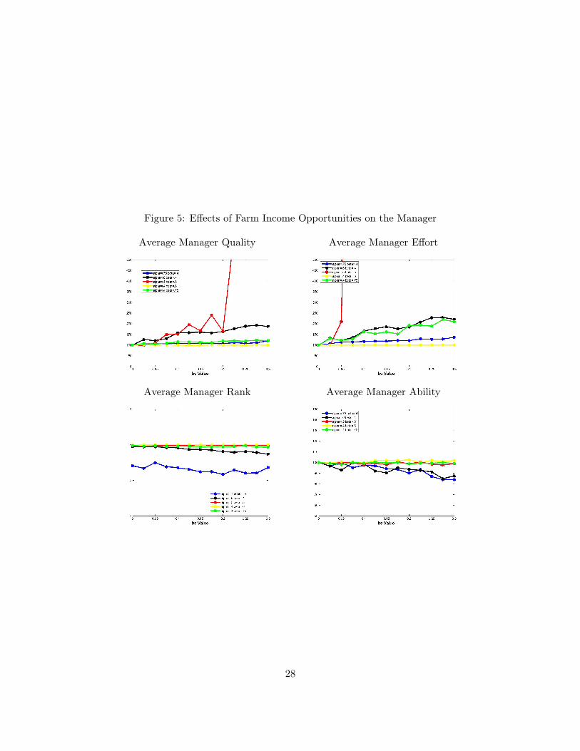
Figure 5: Effects of Farm Income Opportunities on the Manager

Average Manager Quality Average Manager Effort

Average Manager Rank Average Manager Ability

28

Figure 6: Effects on the Candidate Pool

Effects of Off-Farm Income OpportunitiesAverage Pool Quality Average Pool Size

Effects of Farm Income OpportunitiesAverage Pool Quality Average Pool Size

29