Journal of Environmental Science and Water Resources ISSN 2277 0704 Vol. 3(4), pp. 086 - 103, May 2014 2014 Wudpecker Journals

The dynamics of the turbidity maximum zone in a tropical Sabaki estuary in Kenya

Johnson U. Kitheka1, Kennedy M. Mavuti2, Patrick Nthenge3 and Maurice Obiero3

1School of Water Resources Science and Technology, South Eastern Kenya University

P.O Box 170-90200, Kitui, Kenya. 2School of Biological Sciences, University of Nairobi P.O Box 30197-00100, Nairobi, Kenya.

3Kenya Marine and Fisheries Research Institute, P.O Box 81651, Mombasa, Kenya.

*Corresponding author E-mail: Kolbio_kolbio@yahoo.com, jkitheka@seku.ac.ke. Tel: +254 714 645694

Accepted 12 May 2014

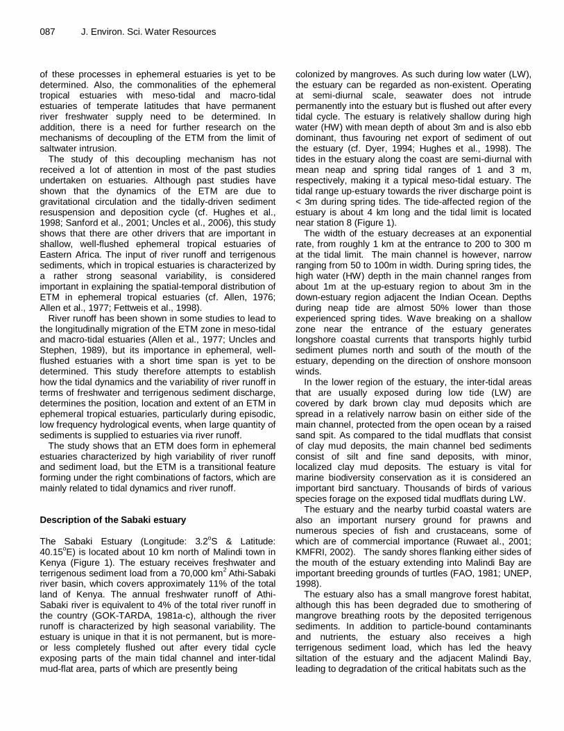
The spatial-temporal variability and the behavior of the Estuarine Turbidity Maximum (ETM) zone in the shallow, ephemeral, well-flushed Sabaki estuary located in the northern region of the Kenya coast, were studied during a period of moderate river discharge. The estuary is one of the most turbid estuaries along the coast of East Africa, characterized by high sediment input and high suspended matter (SPM) concentrations. The estuary is completely flushed after every tidal cycle and experiences high salinity and SPM concentrations gradients at high water (HW). The ETM was generated at HW during periods when the river runoff was near the long-term average (63 m3s-1) and also when it was relatively low (35 m3s-1). The SPM concentrations in the ETM zone varied significantly depending on the river sediment input and phase of the semi-diurnal tide, but were on average 50% greater than the river SPM concentrations. The ETM was also located up-estuary during periods when river runoff was around the long-term average and further down-estuary during periods of low river runoff, due to different sediment settling rates. While gravitational circulation tended to cause accumulation of mud in a null zone located below the freshwater- saltwater interface, causing formation of an ETM zone, the ETM was separated from the salt-limit. This separation was attributed to the time lag in the tidally-driven resuspension of bottom mud and subsequent tidally-driven advection of turbid water up-estuary during the flood period. The relatively low current shear and tidal energy dissipation, combined with high horizontal and vertical gradient in eddy diffusivity in the central region of the estuary, tended to favour rapid settling of flocculated sediments, leading to the formation of an ETM. The ETM zone was formed in the region in which inter-tidal mudflats are located and it is postulated that the formation of the intertidal mudflats is related to that of the ETM dynamics. Key words: Turbidity maximum, river runoff, salt-limit, salinity, suspended particulate matter, Sabaki estuary.

INTRODUCTION Studies on the estuarine turbidity maximum (ETM) zone are important in understanding sedimentary and biological processes in estuaries (Ganju et al., 2004; Islam et al., 2005; Woodruff et al., 2001). In the recent past, there has been a concerted effort towards understanding the sediment transport processes in estuaries and a number of studies have been undertaken focused mainly on unraveling the physical processes responsible for the formation of ETM zones. Most of the previous studies have explained the formation of the ETM zones on the basis of gravitational circulation and tidal asymmetry and there is already a large body of scientific literature in this area (e.g Hughes et al., 1998; Uncles et al., 2001; Uncles et al., 2006; Sanford et al., 2001; Geyer

et al. 2001; Ralston and Geyer, 2009). Unfortunately, there have been very few studies on the tropical estuaries of Africa where freshwater input is highly seasonally variable. The dynamics of the ETM in most of the tropical estuaries of Africa remain largely undocumented despite their important role in influencing coastal processes and productivity. ETM dynamics in estuaries is also thought to influence the formation of mudflats which are important foraging areas for various species of birds, and are also areas that are ideal for establishment of mangrove forests.

Although most of the previous studies have attributed formation of ETM on gravitational circulation and channel bed sediment erosion-deposition cycles, the significance

087 J. Environ. Sci. Water Resources of these processes in ephemeral estuaries is yet to be determined. Also, the commonalities of the ephemeral tropical estuaries with meso-tidal and macro-tidal estuaries of temperate latitudes that have permanent river freshwater supply need to be determined. In addition, there is a need for further research on the mechanisms of decoupling of the ETM from the limit of saltwater intrusion.

The study of this decoupling mechanism has not received a lot of attention in most of the past studies undertaken on estuaries. Although past studies have shown that the dynamics of the ETM are due to gravitational circulation and the tidally-driven sediment resuspension and deposition cycle (cf. Hughes et al., 1998; Sanford et al., 2001; Uncles et al., 2006), this study shows that there are other drivers that are important in shallow, well-flushed ephemeral tropical estuaries of Eastern Africa. The input of river runoff and terrigenous sediments, which in tropical estuaries is characterized by a rather strong seasonal variability, is considered important in explaining the spatial-temporal distribution of ETM in ephemeral tropical estuaries (cf. Allen, 1976; Allen et al., 1977; Fettweis et al., 1998).

River runoff has been shown in some studies to lead to the longitudinally migration of the ETM zone in meso-tidal and macro-tidal estuaries (Allen et al., 1977; Uncles and Stephen, 1989), but its importance in ephemeral, well-flushed estuaries with a short time span is yet to be determined. This study therefore attempts to establish how the tidal dynamics and the variability of river runoff in terms of freshwater and terrigenous sediment discharge, determines the position, location and extent of an ETM in ephemeral tropical estuaries, particularly during episodic, low frequency hydrological events, when large quantity of sediments is supplied to estuaries via river runoff.

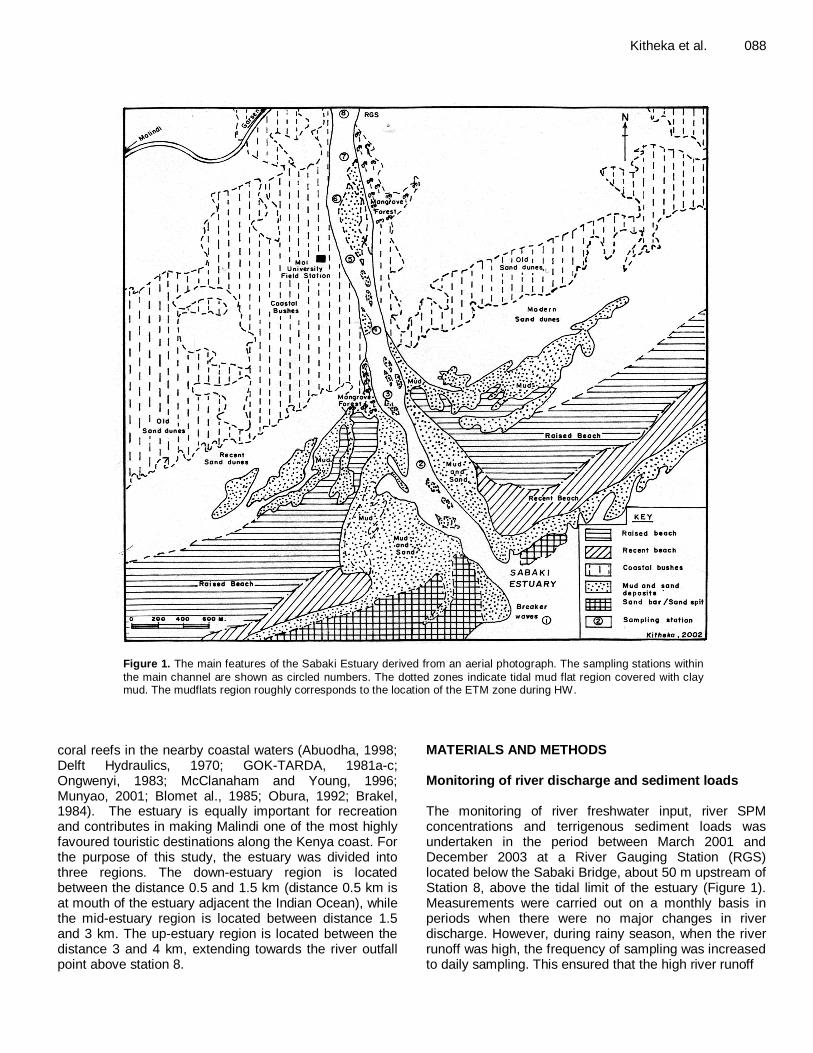
The study shows that an ETM does form in ephemeral estuaries characterized by high variability of river runoff and sediment load, but the ETM is a transitional feature forming under the right combinations of factors, which are mainly related to tidal dynamics and river runoff. Description of the Sabaki estuary The Sabaki Estuary (Longitude: 3.2oS & Latitude: 40.15oE) is located about 10 km north of Malindi town in Kenya (Figure 1). The estuary receives freshwater and terrigenous sediment load from a 70,000 km2 Athi-Sabaki river basin, which covers approximately 11% of the total land of Kenya. The annual freshwater runoff of Athi-Sabaki river is equivalent to 4% of the total river runoff in the country (GOK-TARDA, 1981a-c), although the river runoff is characterized by high seasonal variability. The estuary is unique in that it is not permanent, but is more-or less completely flushed out after every tidal cycle exposing parts of the main tidal channel and inter-tidal mud-flat area, parts of which are presently being

colonized by mangroves. As such during low water (LW), the estuary can be regarded as non-existent. Operating at semi-diurnal scale, seawater does not intrude permanently into the estuary but is flushed out after every tidal cycle. The estuary is relatively shallow during high water (HW) with mean depth of about 3m and is also ebb dominant, thus favouring net export of sediment of out the estuary (cf. Dyer, 1994; Hughes et al., 1998). The tides in the estuary along the coast are semi-diurnal with mean neap and spring tidal ranges of 1 and 3 m, respectively, making it a typical meso-tidal estuary. The tidal range up-estuary towards the river discharge point is < 3m during spring tides. The tide-affected region of the estuary is about 4 km long and the tidal limit is located near station 8 (Figure 1).

The width of the estuary decreases at an exponential rate, from roughly 1 km at the entrance to 200 to 300 m at the tidal limit. The main channel is however, narrow ranging from 50 to 100m in width. During spring tides, the high water (HW) depth in the main channel ranges from about 1m at the up-estuary region to about 3m in the down-estuary region adjacent the Indian Ocean. Depths during neap tide are almost 50% lower than those experienced spring tides. Wave breaking on a shallow zone near the entrance of the estuary generates longshore coastal currents that transports highly turbid sediment plumes north and south of the mouth of the estuary, depending on the direction of onshore monsoon winds.

In the lower region of the estuary, the inter-tidal areas that are usually exposed during low tide (LW) are covered by dark brown clay mud deposits which are spread in a relatively narrow basin on either side of the main channel, protected from the open ocean by a raised sand spit. As compared to the tidal mudflats that consist of clay mud deposits, the main channel bed sediments consist of silt and fine sand deposits, with minor, localized clay mud deposits. The estuary is vital for marine biodiversity conservation as it is considered an important bird sanctuary. Thousands of birds of various species forage on the exposed tidal mudflats during LW.

The estuary and the nearby turbid coastal waters are also an important nursery ground for prawns and numerous species of fish and crustaceans, some of which are of commercial importance (Ruwaet al., 2001; KMFRI, 2002). The sandy shores flanking either sides of the mouth of the estuary extending into Malindi Bay are important breeding grounds of turtles (FAO, 1981; UNEP, 1998).

The estuary also has a small mangrove forest habitat, although this has been degraded due to smothering of mangrove breathing roots by the deposited terrigenous sediments. In addition to particle-bound contaminants and nutrients, the estuary also receives a high terrigenous sediment load, which has led the heavy siltation of the estuary and the adjacent Malindi Bay, leading to degradation of the critical habitats such as the

Kitheka et al. 088

Figure 1. The main features of the Sabaki Estuary derived from an aerial photograph. The sampling stations within the main channel are shown as circled numbers. The dotted zones indicate tidal mud flat region covered with clay mud. The mudflats region roughly corresponds to the location of the ETM zone during HW.

coral reefs in the nearby coastal waters (Abuodha, 1998; Delft Hydraulics, 1970; GOK-TARDA, 1981a-c; Ongwenyi, 1983; McClanaham and Young, 1996; Munyao, 2001; Blomet al., 1985; Obura, 1992; Brakel, 1984). The estuary is equally important for recreation and contributes in making Malindi one of the most highly favoured touristic destinations along the Kenya coast. For the purpose of this study, the estuary was divided into three regions. The down-estuary region is located between the distance 0.5 and 1.5 km (distance 0.5 km is at mouth of the estuary adjacent the Indian Ocean), while the mid-estuary region is located between distance 1.5 and 3 km. The up-estuary region is located between the distance 3 and 4 km, extending towards the river outfall point above station 8.

MATERIALS AND METHODS Monitoring of river discharge and sediment loads The monitoring of river freshwater input, river SPM concentrations and terrigenous sediment loads was undertaken in the period between March 2001 and December 2003 at a River Gauging Station (RGS) located below the Sabaki Bridge, about 50 m upstream of Station 8, above the tidal limit of the estuary (Figure 1). Measurements were carried out on a monthly basis in periods when there were no major changes in river discharge. However, during rainy season, when the river runoff was high, the frequency of sampling was increased to daily sampling. This ensured that the high river runoff

089 J. Environ. Sci. Water Resources events were captured in our data. River discharges were measured using the cross-sectional-area-velocity approach (Linsley et al., 1988). The depth-averaged river flow current speeds at three points within the river cross-section were integrated to obtain the mean velocities, which were subsequently multiplied with the corresponding river cross-sectional areas to obtain instantaneous river discharge rates (Chapman, 1996; Bartram and Balance, 1996). Instantaneous river discharge rates were then used to compute freshwater input into the estuary at times when longitudinal and vertical surveys on SPM concentrations, salinities, tidal elevations and tidal current speeds were undertaken in the estuary.

For the determination of river SPM concentrations and sediment loads, the water samples were drawn at the middle of the main channel of the river, using a Niskin Sampler. The water samples were drawn at four (4) points within the water column, at 0.2h, 0.4h, 0.6h and 0.8h, where h is the total water depth. Samples of water-sediment mixture were analysed at the Kenya Marine and Fisheries Research Institute (KMFRI) marine environmental studies laboratory in Mombasa.

The analysis involved the determination of SPM concentrations through filtration using Whatman GF filters according to APHA (1992) methods. The river sediment loads (kgs-1) were calculated by integrating the product of the instantaneous river discharges (m3s-1) with the corresponding river SPM concentrations (kgm3). The vertically integrated river SPM concentrations occurring during the time between two river gauging events were extrapolated according to constant concentration and constant flux approaches described in Chapman (1996). Monitoring the SPM concentration, tidal elevation and current velocities A field monitoring campaign aimed at establishing the horizontal and vertical distribution of SPM concentrations, ebb and flood tide current velocities and tidal elevations was undertaken in the estuary. The variability of the SPM concentrations was monitored using a turbidity sensor fitted on an Aanderaa Recording Current Meter (RCM-9). One RCM-9 with the turbidity sensor attached to it, was moored at stations 3 and 4 (Figure 1) at a distance of about 1.5 km and 2 km, respectively from the mouth of the estuary.

The instrument was moored in different stations within the estuary for up to 3 days, in the period between 28th and 30th January 2002 and also in the period between 12th and 15th June 2003. Both the RCM-9 and turbidity sensor were programmed to log in current velocities (including directions) and turbidity at interval of 5 minutes. Water levels were measured using divers’ pressure gauges mounted on a RCM-9, which also logged in water level data at intervals of 5 minutes for up to a period of 3

days. The RCM-9 and turbidity sensor were considered important in the determination of temporary patterns of variability of SPM concentrations within a tidal cycle, including the determination of the relationship between the variability of SPM concentrations and tidal dynamics. Determination of vertical and horizontal distribution of salinity and SPM concentrations Using a fast inflatable boat (rubber dinghy), spot measurements were carried out during HW in all 8 stations established in the estuary in order to determine the spatial and vertical distribution of salinity and SPM concentrations. The 8 sampling stations were located at every 0.5 km from the limit of salt intrusion up to the entrance of the estuary bordering the Indian Ocean (Figure 1).

Water-sediment mixture samples were drawn using a Niskin sampler at 0.2h, 0.4h, 0.6h and 0.8h to determine the vertical distribution of SPM concentrations, where h is the local depth. The determination of SPM concentrations involved the filtration of water-sediment mixture in the laboratory using Whatman GF filters according to APHA (1992) methods. Salinity was measured in situ at intervals of 0.2m up to near the channel bottom, by lowering a probe attached to a long cable connected to a hand-held Aanderaa Salinometer. Salinity was expressed in terms of Practical Salinity Units (PSU).

The data on the vertical and horizontal distributions of salinity and SPM concentrations were used to construct contour profiles whose analysis provided information on the distribution of ETM with respect to horizontal and vertical distribution of SPM concentrations and salinities in the estuary during periods of different tidal ranges, river discharges of freshwater and sediment loads. The contour profiles were also analysed in order to establish the extent of decoupling of the ETM from the landward extent of the limit of salt intrusion, during ebb and flood tides. RESULTS River runoff and sediment input in the Sabaki estuary The input of freshwater and terrigenous sediments into the Sabaki estuary is highly seasonally variable and this has implications on the level of salinities and SPM concentrations in the estuary. Figure 2 shows the patterns of variability of monthly averaged daily river discharges measured at a river gauging station located near station 8. The freshwater input in to the estuary during the period of this study varied from 30m3s-1 to 680 m3s-1, representing river flows that can be considered moderate since during the years of the El Nino Southern Oscillation phenomena, the flood flow discharges can be

Kitheka et al. 090

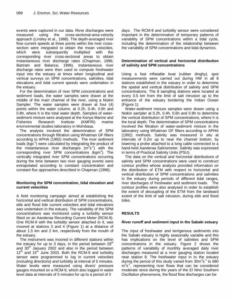
Figure 2. The monthly averaged instantaneous river discharges and SPM concentrations in the period between January 2001 and December 2003. The periods of low frequency, high river runoff events, are shown as the peaks in river discharges.

as high as 1,000 m3s-1. These extreme river runoffs are however, usually experienced for a relatively short period of few days. The mean river discharge was of the order 70 m3s-1 and the river flows < 70 m3s-1 were more frequent as they occurred in 90% of the time. The flows that were > 150 m3s-1 had a relatively low frequency of occurrence as they usually occurred in < 10% of the time, mainly during the rainy season, particularly during the South-East Monsoon. Also, most of the terrigenous sediment input into the estuary occurred during infrequent high river discharge events during rainy season. Good example of these low frequency events are the peak river runoffs experienced in April-May as shown in Figure 2.

The Sabaki river discharges a high sediment load into the estuary. During the period of the study, the sediment load ranged from 30 tons.day-1 during periods of low river runoff to 133,000 tons.day-1 during periods of high river runoff, largely in flood events. The river SPM concentrations generally exhibited high variability as they ranged from 0.3 to 3.0 gl-1.

The relationship between river runoff and river SPM concentrations was such that at the beginning of the rainy season, the relatively low river discharges were

characterized by high SPM concentrations as compared to those experienced during moderate and high river runoff at the later stages of the rainy season. Main tidal features and characteristics The Sabaki estuary experiences semi-diurnal tides with two low and high waters after every 25 hour period. The tidal elevations measured at stations 3 and 4, about 2 km from the mouth of the estuary, showed that the spring tidal range is 3.0 m and the neap tidal range is of the order of 1.0 m. There is a significant reduction in tidal amplitude up-estuary that is attributed to frictional losses that occur as the tidal wave is propagated in the relatively shallow waters of the estuary with depths <3 m (see also Friedrichs et al., 1992; Uncles et al., 2006).

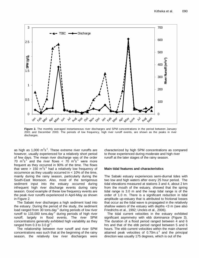
The tidal current velocities in the estuary exhibited significant asymmetry with ebb dominance (Figure 3). The duration of a flood period ranged between 4 and 6 hrs and that of the ebb period ranged between 5 and 6 hours. The ebb current velocities within the main channel attained peak velocities of 0.70m.s-1 and the principal direction was usually 175 degrees, which is out of the

0

100

200

300

400

500

600

700

0

0.5

1

1.5

2

2.5

3

Rive

r Run

off (

m3 s

-1)

SPM

(g/l

)

TSSC Discharge

091 J. Environ. Sci. Water Resources

Figure 3. The ebb and flood tide current velocities and current direction at station 3, about 1.5 km from mouth of the estuary. True north is zero degree. Counting of degrees is clockwise.

estuary towards the Indian Ocean. The flood current velocities attained peak velocities of 0.30 m.s-1 and were mainly directed at 325 degrees within the main channel (Figure 3). The relatively stronger ebb current velocities, as compared to flood current velocities were attributed to the reinforcement of the ebb current by the river flow during ebb tide. Previous studies elsewhere have shown that the ebb-dominance has a tendency of inducing net export of sediments out of estuaries (cf. Wolanskiet al., 1998; Wolanskiet al., 2001). Current shear and the variations of SPM concentrations within the tidal cycle The tidal energy dissipation and current shear plays an important part in the sediment erosion – deposition cycle, and therefore determination of their magnitudes was considered vital in the study of ETM dynamics in estuaries. The bulk indicator of tidal energy dissipation was computed as U3/h while the current shear was computed as U/h where U is the depth-averaged current velocity and h is the depth.

These two parameters provided indications on the variability of current shear stresses within a tidal cycle and the capacity of the current to erode and transport fine bottom sediments (See also Uncles et al., 2006). Field data showed that in a tidal cycle, the current shear increases significantly at the early flood tide period (Figure 4).

However, it decreases during the late flood tide period, HW and during early ebb tide period where it ranged 0.03

and 0.09 s-1. During ebb period, the current shear was generally high reaching maximum at LW (3.2 to 3.8 s-1). An increase in current shear resulted into an increase in SPM concentrations as shown in Figure 4, which is an indication of channel bed-sediment erosion.

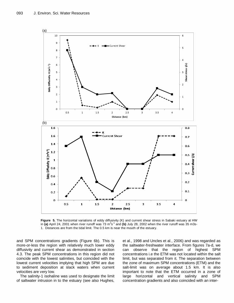
Figure 5 shows the horizontal distribution of current shear and eddy diffusivity (K) based on measurements undertaken at HW in April 2001 and July 2002. The April 2001 measurements were undertaken during a period of average river runoff of the order 70 m3s-1, and it was evident that down-estuary region fronting the ocean had high current shear and high eddy diffusivity as compared to the middle region of the estuary, which was characterized by relatively low current shear and eddy diffusivity.

However, the situation was different when there was low river runoff of the order 35 m3s-1. In both the up-estuary and down-estuary regions towards the river mouth and the open ocean, respectively, both the current shears and eddy diffusivities were relatively higher during a period of low river runoff. However, there were of much lower magnitude as compared to those experienced during the periods of average or high river runoff (Figure 5a-b).

The current shear and eddy diffusivities were almost 10 times larger during periods of average river runoff as compared to periods of low river runoff. As will be shown later, this has an implication on the extent of the ETM in the estuary.

The results of measurements of SPM concentrations over two tidal cycles at every 5-min interval during a 2.5 m tidal range spring tide, in a period of relatively low river

50 100 150 200 250 300 3500

0.1

0.2

0.3

0.4

0.5

0.6

0.7

Direc tion(degr.)

Vel

ocity

(m/s

)

Kitheka et al. 092

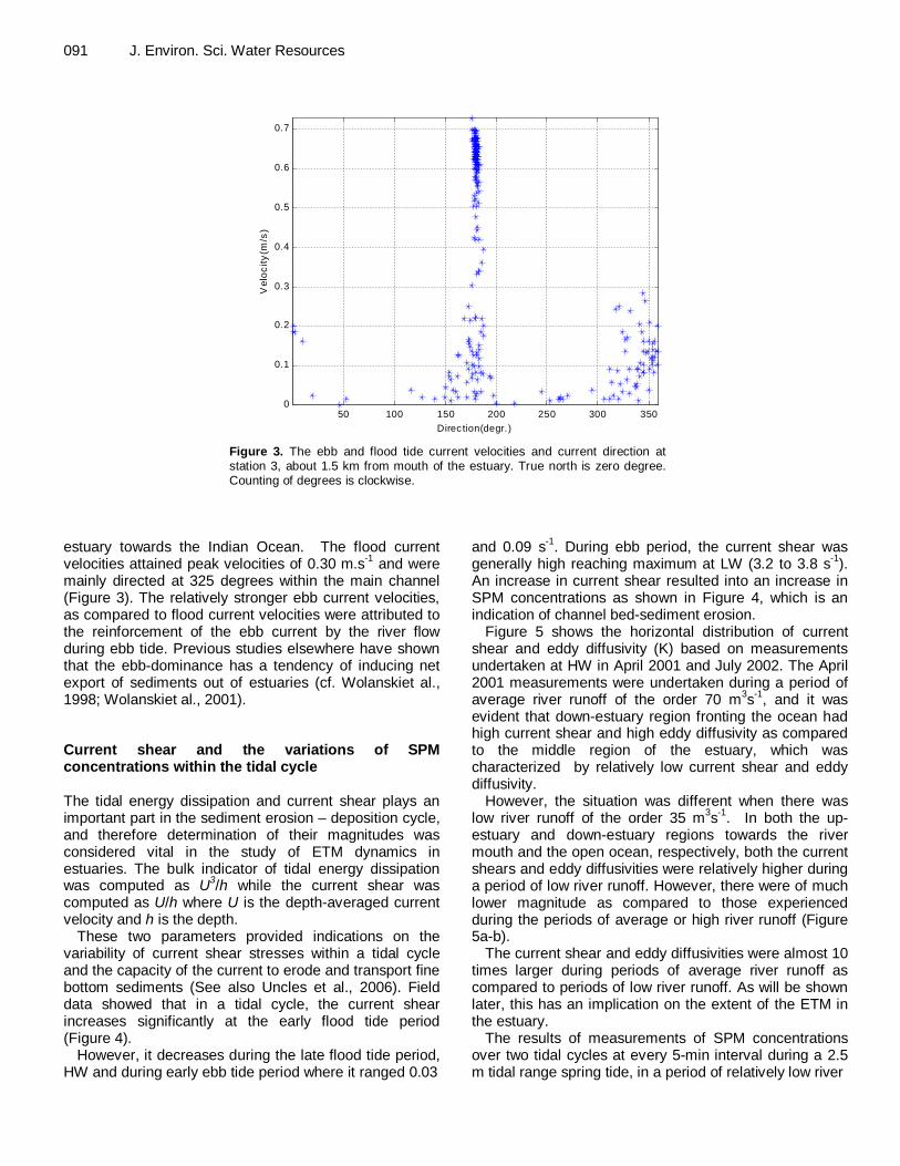
Figure 4. Time-series plot of current velocities (U), tidal elevation (h), current shear (U/h), tidal energy dissipation (U3/h) and SPM concentrations, based on measurements at station 3 located, about 2 km from the mouth of the Sabaki estuary, in the period 28-30 January 2002. The river runoff was 35 m3s-1.

discharge of 35 m3.s-1 showed that during low tide (LW), SPM concentrations in the main channel were relatively high ranging from 0.75 to 5.0 g.l-1.

The high SPM concentrations in the main channel at the late stages of ebb tide and during LW were essentially riverine since during this period, the seawater had already been flushed out the estuary and the river runoff dominated in the main channel where the RCM-9 and the turbidity sensor were moored. There was however resuspension of the channel bed clay mud that had been deposited during the previous HW slack. The resuspension of bottom sediments was attributed to high current shear associated river–induced current velocities of the order 70 ms-1, which were well above the threshold required for resuspending the fine bottom sediments. Thus, the combined effect of the river runoff SPM and resuspension of the bottom mud in the main channel led high turbidity in the main channel at low tide. However, it is important to note that during early stages of flood tide, there was a rapid decrease in SPM concentrations from 1.0 g.l-1 to about 0.15 g.l-1 as seawater entered into the estuary pushing the river water upstream (Figure 4).

Subsequently, the SPM concentrations decreased as the tidal elevation increased during flood tide, attaining the lowest levels during HW slack when the current velocities were sluggish. This allowed for rapid deposition of fine clay sediments into the channel bottom as well as the inter-tidal areas, since these areas are flooded with seawater during high tide. It can be concluded from these

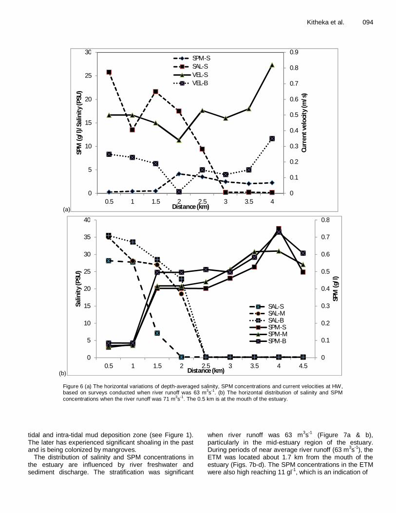
results that the SPM concentrations were generally high during late stages of ebb period and low tide and also during early stages of flood period. The high SPM concentrations during early stages of flood period were attributed to the resuspension of the fine mud sediment deposits at the channel bed and also due turbulence in the down-estuary region that results as the turbid river runoff meets the seawater flowing back into the estuary during flood tide. Horizontal and vertical variations of salinity and SPM concentrations A significant horizontal and vertical variation in the distribution of salinities and SPM concentrations was observed in the Sabaki estuary. Figure 6(a) shows the horizontal variations of depth-averaged salinity and SPM concentrations based on measurements undertaken at high tide (HW). The horizontal variations represent changes in the

depth-averaged salinities and SPM concentrations with distance from the mouth of the estuary up to the tidal limit located at station 8. Figure 6b shows both the vertical and horizontal distributions of the same parameters during a period of average river runoff of 63 m3s-1. It was observed that the mid-estuary region located at a distance of between 1.5 and 3 km from the mouth of the estuary had relatively large horizontal and vertical salinity

093 J. Environ. Sci. Water Resources

(a)

(b)

Figure 5. The horizontal variations of eddy diffusivity (K) and current shear stress in Sabaki estuary at HW in (a) April 24, 2001 when river runoff was 73 m3s-1 and (b) July 28, 2002 when the river runoff was 35 m3s-1. Distances are from the tidal limit. The 0.5 km is near the mouth of the estuary.

and SPM concentrations gradients (Figure 6b). This is more-or-less the region with relatively much lower eddy diffusivity and current shear as demonstrated in section 4.3. The peak SPM concentrations in this region did not coincide with the lowest salinities, but coincided with the lowest current velocities implying that high SPM are due to sediment deposition at slack waters when current velocities are very low.

The salinity-1 isohaline was used to designate the limit of saltwater intrusion in to the estuary (see also Hughes,

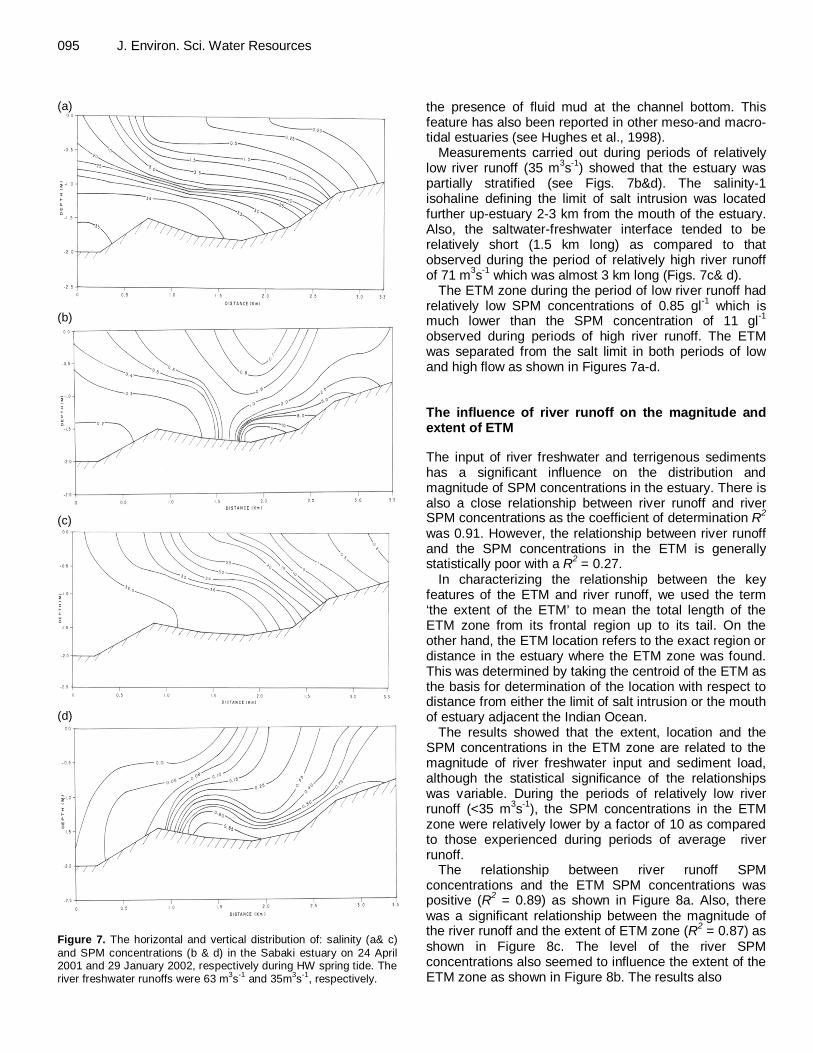
et al., 1998 and Uncles et al., 2006) and was regarded as the saltwater-freshwater interface. From figures 7a-d, we can observe that the region of highest SPM concentrations i.e the ETM was not located within the salt limit, but was separated from it. The separation between the zone of maximum SPM concentrations (ETM) and the salt-limit was on average about 1.5 km. It is also important to note that the ETM occurred in a zone of large horizontal and vertical salinity and SPM concentration gradients and also coincided with an inter-

Kitheka et al. 094

(a)

(b) Figure 6 (a) The horizontal variations of depth-averaged salinity, SPM concentrations and current velocities at HW, based on surveys conducted when river runoff was 63 m3s-1. (b) The horizontal distribution of salinity and SPM concentrations when the river runoff was 71 m3s-1. The 0.5 km is at the mouth of the estuary.

tidal and intra-tidal mud deposition zone (see Figure 1). The later has experienced significant shoaling in the past and is being colonized by mangroves.

The distribution of salinity and SPM concentrations in the estuary are influenced by river freshwater and sediment discharge. The stratification was significant

when river runoff was 63 m3s-1 (Figure 7a & b), particularly in the mid-estuary region of the estuary. During periods of near average river runoff (63 m3s-1), the ETM was located about 1.7 km from the mouth of the estuary (Figs. 7b-d). The SPM concentrations in the ETM were also high reaching 11 gl-1, which is an indication of

0

0.1

0.2

0.3

0.4

0.5

0.6

0.7

0.8

0.9

0

5

10

15

20

25

30

0.5 1 1.5 2 2.5 3 3.5 4

Curr

ent v

eloc

ity (m

/s)

SPM

(g/l

)/Sa

linity

(PSU

)

Distance (km)

SPM-SSAL-SVEL-SVEL-B

0

0.1

0.2

0.3

0.4

0.5

0.6

0.7

0.8

0

5

10

15

20

25

30

35

40

0.5 1 1.5 2 2.5 3 3.5 4 4.5

SPM

(g/l

)

Salin

ity (P

SU)

Distance (km)

SAL-SSAL-MSAL-BSPM-SSPM-MSPM-B

095 J. Environ. Sci. Water Resources (a)

(b)

(c)

(d)

Figure 7. The horizontal and vertical distribution of: salinity (a& c) and SPM concentrations (b & d) in the Sabaki estuary on 24 April 2001 and 29 January 2002, respectively during HW spring tide. The river freshwater runoffs were 63 m3s-1 and 35m3s-1, respectively.

the presence of fluid mud at the channel bottom. This feature has also been reported in other meso-and macro-tidal estuaries (see Hughes et al., 1998).

Measurements carried out during periods of relatively low river runoff (35 m3s-1) showed that the estuary was partially stratified (see Figs. 7b&d). The salinity-1 isohaline defining the limit of salt intrusion was located further up-estuary 2-3 km from the mouth of the estuary. Also, the saltwater-freshwater interface tended to be relatively short (1.5 km long) as compared to that observed during the period of relatively high river runoff of 71 m3s-1 which was almost 3 km long (Figs. 7c& d).

The ETM zone during the period of low river runoff had relatively low SPM concentrations of 0.85 gl-1 which is much lower than the SPM concentration of 11 gl-1 observed during periods of high river runoff. The ETM was separated from the salt limit in both periods of low and high flow as shown in Figures 7a-d. The influence of river runoff on the magnitude and extent of ETM The input of river freshwater and terrigenous sediments has a significant influence on the distribution and magnitude of SPM concentrations in the estuary. There is also a close relationship between river runoff and river SPM concentrations as the coefficient of determination R2 was 0.91. However, the relationship between river runoff and the SPM concentrations in the ETM is generally statistically poor with a R2 = 0.27.

In characterizing the relationship between the key features of the ETM and river runoff, we used the term ‘the extent of the ETM’ to mean the total length of the ETM zone from its frontal region up to its tail. On the other hand, the ETM location refers to the exact region or distance in the estuary where the ETM zone was found. This was determined by taking the centroid of the ETM as the basis for determination of the location with respect to distance from either the limit of salt intrusion or the mouth of estuary adjacent the Indian Ocean.

The results showed that the extent, location and the SPM concentrations in the ETM zone are related to the magnitude of river freshwater input and sediment load, although the statistical significance of the relationships was variable. During the periods of relatively low river runoff (<35 m3s-1), the SPM concentrations in the ETM zone were relatively lower by a factor of 10 as compared to those experienced during periods of average river runoff.

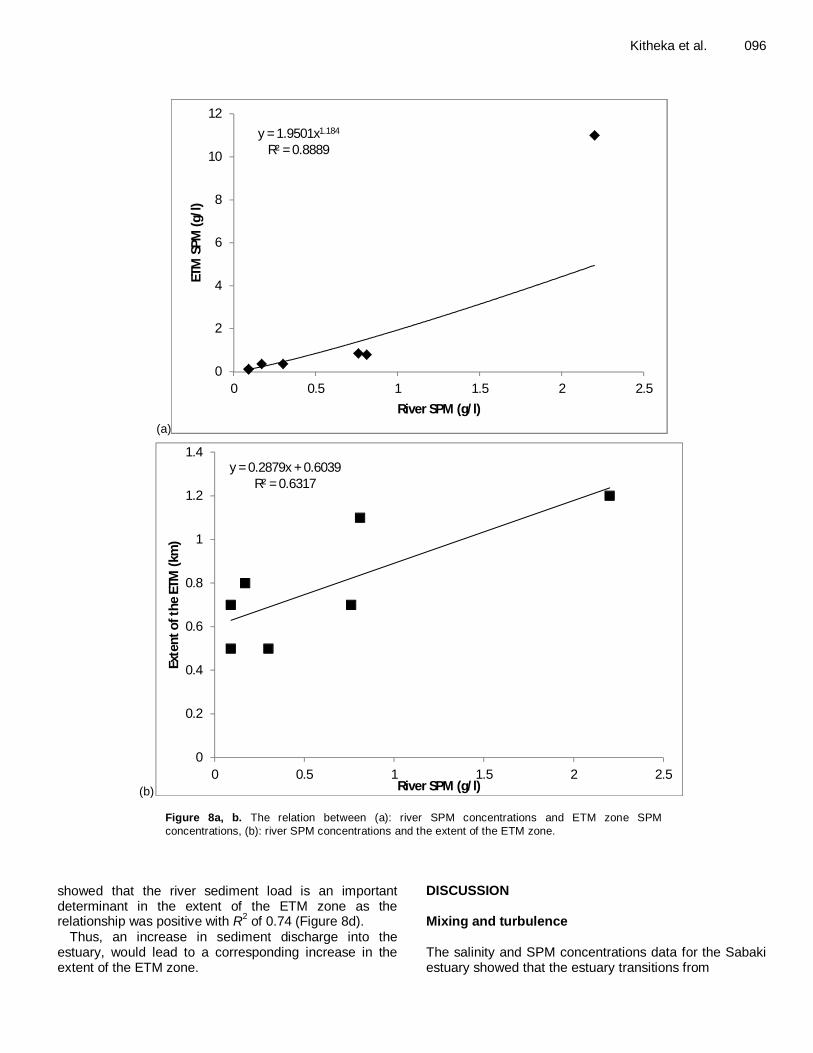
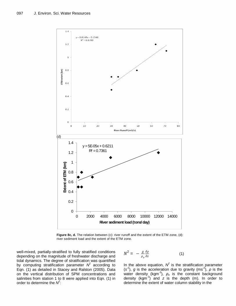
The relationship between river runoff SPM concentrations and the ETM SPM concentrations was positive (R2 = 0.89) as shown in Figure 8a. Also, there was a significant relationship between the magnitude of the river runoff and the extent of ETM zone (R2 = 0.87) as shown in Figure 8c. The level of the river SPM concentrations also seemed to influence the extent of the ETM zone as shown in Figure 8b. The results also

Kitheka et al. 096

(a)

(b) Figure 8a, b. The relation between (a): river SPM concentrations and ETM zone SPM concentrations, (b): river SPM concentrations and the extent of the ETM zone.

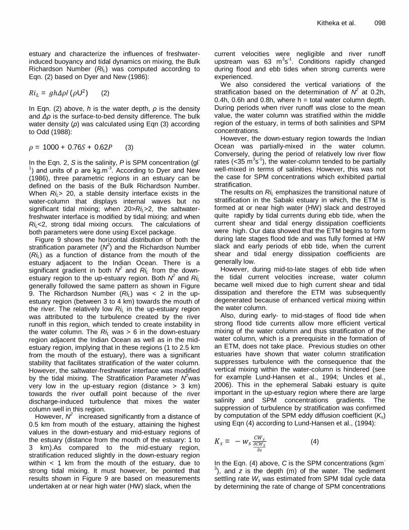
showed that the river sediment load is an important determinant in the extent of the ETM zone as the relationship was positive with R2 of 0.74 (Figure 8d).

Thus, an increase in sediment discharge into the estuary, would lead to a corresponding increase in the extent of the ETM zone.

DISCUSSION Mixing and turbulence The salinity and SPM concentrations data for the Sabaki estuary showed that the estuary transitions from

y = 1.9501x1.184

R² = 0.8889

0

2

4

6

8

10

12

0 0.5 1 1.5 2 2.5

ETM

SPM

(g/l

)

River SPM (g/l)

y = 0.2879x + 0.6039R² = 0.6317

0

0.2

0.4

0.6

0.8

1

1.2

1.4

0 0.5 1 1.5 2 2.5

Exte

nt o

f the

ETM

(km

)

River SPM (g/l)

097 J. Environ. Sci. Water Resources

(d)

Figure 8c, d. The relation between (c): river runoff and the extent of the ETM zone, (d): river sediment load and the extent of the ETM zone.

well-mixed, partially-stratified to fully stratified conditions depending on the magnitude of freshwater discharge and tidal dynamics. The degree of stratification was quantified by computing stratification parameter N2 according to Eqn. (1) as detailed in Stacey and Ralston (2005). Data on the vertical distribution of SPM concentrations and salinities from station 1 to 8 were applied into Eqn. (1) in order to determine the N2:

푁2 = − 푔휌표휕휌휕푧 (1)

In the above equation, N2 is the stratification parameter (s-2), g is the acceleration due to gravity (ms-2), ρ is the water density (kgm-3), ρo is the constant background density (kgm-3) and z is the depth (m). In order to determine the extent of water column stability in the

y = 5E-05x + 0.6211R² = 0.7361

0

0.2

0.4

0.6

0.8

1

1.2

1.4

0 2000 4000 6000 8000 10000 12000 14000

Exte

nt o

f ETM

(km

)

River sediment load (tons/day)

estuary and characterize the influences of freshwater-induced buoyancy and tidal dynamics on mixing, the Bulk Richardson Number (RiL) was computed according to Eqn. (2) based on Dyer and New (1986): 푅푖 = 푔ℎ훥휌/(휌U ) (2) In Eqn. (2) above, h is the water depth, ρ is the density and Δρ is the surface-to-bed density difference. The bulk water density (ρ) was calculated using Eqn (3) according to Odd (1988): 휌 = 1000 + 0.76푆 + 0.62푃 (3) In the Eqn. 2, S is the salinity, P is SPM concentration (gl-1) and units of ρ are kg.m-3. According to Dyer and New (1986), three parametric regions in an estuary can be defined on the basis of the Bulk Richardson Number. When RiL> 20, a stable density interface exists in the water-column that displays internal waves but no significant tidal mixing; when 20>RiL>2, the saltwater-freshwater interface is modified by tidal mixing; and when RiL<2, strong tidal mixing occurs. The calculations of both parameters were done using Excel package.

Figure 9 shows the horizontal distribution of both the stratification parameter (N2) and the Richardson Number (RiL) as a function of distance from the mouth of the estuary adjacent to the Indian Ocean. There is a significant gradient in both N2 and RiL from the down-estuary region to the up-estuary region. Both N2 and RiL generally followed the same pattern as shown in Figure 9. The Richardson Number (RiL) was < 2 in the up-estuary region (between 3 to 4 km) towards the mouth of the river. The relatively low RiL in the up-estuary region was attributed to the turbulence created by the river runoff in this region, which tended to create instability in the water column. The RiL was > 6 in the down-estuary region adjacent the Indian Ocean as well as in the mid-estuary region, implying that in these regions (1 to 2.5 km from the mouth of the estuary), there was a significant stability that facilitates stratification of the water column. However, the saltwater-freshwater interface was modified by the tidal mixing. The Stratification Parameter N2was very low in the up-estuary region (distance > 3 km) towards the river outfall point because of the river discharge-induced turbulence that mixes the water column well in this region.

However, N2 increased significantly from a distance of 0.5 km from mouth of the estuary, attaining the highest values in the down-estuary and mid-estuary regions of the estuary (distance from the mouth of the estuary: 1 to 3 km).As compared to the mid-estuary region, stratification reduced slightly in the down-estuary region within < 1 km from the mouth of the estuary, due to strong tidal mixing. It must however, be pointed that results shown in Figure 9 are based on measurements undertaken at or near high water (HW) slack, when the

Kitheka et al. 098 current velocities were negligible and river runoff upstream was 63 m3s-1. Conditions rapidly changed during flood and ebb tides when strong currents were experienced.

We also considered the vertical variations of the stratification based on the determination of N2 at 0.2h, 0.4h, 0.6h and 0.8h, where h = total water column depth. During periods when river runoff was close to the mean value, the water column was stratified within the middle region of the estuary, in terms of both salinities and SPM concentrations.

However, the down-estuary region towards the Indian Ocean was partially-mixed in the water column. Conversely, during the period of relatively low river flow rates (<35 m3s-1), the water-column tended to be partially well-mixed in terms of salinities. However, this was not the case for SPM concentrations which exhibited partial stratification.

The results on RiL emphasizes the transitional nature of stratification in the Sabaki estuary in which, the ETM is formed at or near high water (HW) slack and destroyed quite rapidly by tidal currents during ebb tide, when the current shear and tidal energy dissipation coefficients were high. Our data showed that the ETM begins to form during late stages flood tide and was fully formed at HW slack and early periods of ebb tide, when the current shear and tidal energy dissipation coefficients are generally low.

However, during mid-to-late stages of ebb tide when the tidal current velocities increase, water column became well mixed due to high current shear and tidal dissipation and therefore the ETM was subsequently degenerated because of enhanced vertical mixing within the water column.

Also, during early- to mid-stages of flood tide when strong flood tide currents allow more efficient vertical mixing of the water column and thus stratification of the water column, which is a prerequisite in the formation of an ETM, does not take place. Previous studies on other estuaries have shown that water column stratification suppresses turbulence with the consequence that the vertical mixing within the water-column is hindered (see for example Lund-Hansen et al., 1994; Uncles et al., 2006). This in the ephemeral Sabaki estuary is quite important in the up-estuary region where there are large salinity and SPM concentrations gradients. The suppression of turbulence by stratification was confirmed by computation of the SPM eddy diffusion coefficient (Ks) using Eqn (4) according to Lund-Hansen et al., (1994): 퐾푠 = −푤푠

퐶푊푠휕퐶푊푠휕푧

(4)

In the Eqn. (4) above, C is the SPM concentrations (kgm-

3), and z is the depth (m) of the water. The sediment settling rate Ws was estimated from SPM tidal cycle data by determining the rate of change of SPM concentrations

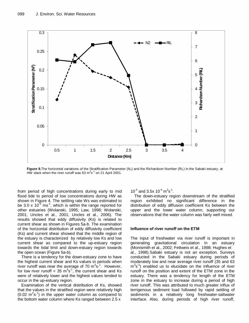
099 J. Environ. Sci. Water Resources

Figure 9.The horizontal variations of the Stratification Parameter (N2) and the Richardson Number (RiL) in the Sabaki estuary, at HW slack when the river runoff was 63 m3s-1 on 21 April 2001.

from period of high concentrations during early to mid flood tide to period of low concentrations during HW as shown in Figure 4. The settling rate Ws was estimated to be 3.0 x 10-3 ms-1, which is within the range reported for other estuaries (Wolanski, 1995; Law, 1998; Wolanski, 2001; Uncles et al., 2001; Uncles et al., 2006). The results showed that eddy diffusivity (Ks) is related to current shear as shown in Figures 5a-b. The examination of the horizontal distribution of eddy diffusivity coefficient (Ks) and current shear showed that the middle region of the estuary is characterized by relatively low Ks and low current shear as compared to the up-estuary region towards the tidal limit and down-estuary region towards the open ocean (Figure 5a-b).

There is a tendency for the down-estuary zone to have the highest current shear and Ks values in periods when river runoff was near the average of 70 m3s-1. However, for low river runoff < 35 m3s-1, the current shear and Ks were of relatively lower and the highest values tended to occur in the up-estuary region.

Examination of the vertical distribution of Ks, showed that the values in the stratified region were relatively high (0.02 m2s-1) in the upper water column as compared to the bottom water column where Ks ranged between 2.5 x

10-4 and 3.5x 10-4 m2s-1. The down-estuary region downstream of the stratified

region exhibited no significant difference in the distribution of eddy diffusion coefficient Ks between the upper and the lower water column, supporting our observations that the water column was fairly well mixed. Influence of river runoff on the ETM The input of freshwater via river runoff is important in generating gravitational circulation in an estuary (Monismith et al., 2002; Fettweis et al., 1998; Hughes et al., 1998).Sabaki estuary is not an exception. Surveys conducted in the Sabaki estuary during periods of moderately low and near average river runoff (35 and 63 m3s-1) enabled us to elucidate on the influence of river runoff on the position and extent of the ETM zone in the estuary. There was a tendency for length of the ETM zone in the estuary to increase during a period of high river runoff. This was attributed to much greater influx of terrigenous sediment load followed by rapid settling of sediments in a relatively long freshwater-saltwater interface. Also, during periods of high river runoff,

0

1

2

3

4

5

6

7

8

0

0.05

0.1

0.15

0.2

0.25

0.3

0.5 1 1.5 2 2.5 3 3.5 4

Rich

ards

on N

umbe

r (Ri

L)

Stra

tific

atio

n Pa

ram

eter

(N2 )

Distance (Km)

N2 RiL

longitudinal salinity gradient was much higher (11 PSU.km-1) which allowed for increased intrusion of seawater upstream during flood tide (cf. Monismith et al., 2002). It should also be noted that during periods of high river runoff and high sediment load, there is a relatively greater seawater-freshwater interface through which sediments were flocculated and subsequently deposited in the null zone (Figures 7a-d), although this occurred within a short period time within the tidal cycle.

The distance of the ETM zone measured from its core region (where SPM concentration is the highest) to the mouth of the estuary, increased during the period of near average river runoff and decreased during the period of low river runoff.During periods of low runoff, the ETM region was located much closer to the mouth of the estuary, and during periods of near average river runoff, it was located further up-estuary towards the salt limit. It can also be noted that during periods of near average river runoff, the well-developed salinity stratification at HW meant that the freshwater-seawater interface was long (1 to 2 km) which, provided a large surface through which the flocculated sediments settled to the bottom water column (cf. Wolanski, 1995; Law, 1998; Wolanskiet al., 1998; Uncles et al., 2001; Uncles et al., 2006). This led to an ETM of much greater horizontal extent. Fettweis et al., (1998) working in the Scheldt estuary in Belgium reported that the seasonally varying freshwater discharge determines the position of the turbidity maximum.

Despite the fact that Scheldt estuary is fundamentally different from the Sabaki estuary, similar observations on the effects of river discharge were made in the Sabaki estuary. There were however significant differences in the position of ETM zone under varying river runoff conditions, ranging between 0.3 and 1 km from the mouth of the estuary.

It is argued that these differences are due to variations of the grain-sizes of sediment particles transported by the river, in that during moderately high runoff, the river usually was characterized by high velocities > 1 ms-1 and therefore had much greater capacity to transport relatively large-sized sediment particles that have relatively higher settling velocity.

This resulted in rapid deposition of fine sediments in the up-estuary region towards the tidal limit. However, during low river runoff, the river transported relativelyfiner sediment particles that remained in suspension for a relatively longer period. The fine sediments were therefore transported further down-estuary where settling took place at HW slack. Sandford et al. (2001) working on Chesapeake Bay reported findings that agrees with our observations in the Sabaki estuary. Our findings also indicate that the river runoff is important in determining the size of the ETM zone in the estuary. The size of the ETM zone was much larger, of the order 1.5 km during the periods of near average river runoff and was relatively smaller<0.5 km during periods of low river runoff. These differences can also be attributed to the

Kitheka et al. 100 variations in the sediment particle grain sizes, the magnitude of the river sediment load as well as the length of the salt-limit which is a function of tidal range.

The SPM concentrations in the ETM core zone were generally of the same order of magnitude as the river runoff SPM concentration (Figure 8a). However, there was a tendency for the SPM concentration in the ETM zone to be relatively higher than that in the river runoff during periods of high river runoff. In most cases, the difference between the river SPM concentrations and the ETM SPM concentrations was less than 30% in periods of low river runoff and was relatively higher (80%) during periods when river runoff and sediment load were high.

However, the difference between the river SPM concentrations and the ETM zone SPM concentrations was attributed to the resuspension of the channel bed sediments that adds more fine sediments to the water column leading to the relatively higher SPM concentrations in the ETM zone. Relatively higher SPM concentrations during periods of moderate to high river runoff means large volume of sediments are deposited within the channel bed at HW and consequently greater volume of sediments are available for resuspension during early stages of flood period and late stages of ebb period.

Equally important is sediment load which also determines the extent of the ETM zone (Figure 8d). Surprisingly, these results were consistent with findings of studies carried out in permanent estuaries that are significantly different from the ephemeral Sabaki estuary (e.g. Geyer, 1993; Monismith et al., 2002; Ralston et al., 2010).

These findings on the existence of a positive relationship between river runoff and the extent of ETM zone, means that although ETM zone is a transient feature in ephemeral estuaries, it is subject to the seasonal cycles of river runoff and sediment input into the estuary (see also Uncles et al., 1994). Formation and separation of the ETM from the salt limit The ETM zone in the Sabaki estuary is more-or lesslocated within the region where the inter-tidal and sub-tidal mud deposition basins are located in the estuary (see Figure 1).This zone, which is shallow < 2m during HW and is exposed during LW, has experienced significant net clay mud accumulation in the past years and in some places is being colonized by mangroves.

Thus, there is every possibility that the formation of the sub-tidal and inter-tidal mudflats is related to the accumulation of fine sediments in the ETM during HW. The formation of ETM zone in the ephemeral Sabaki estuary can be explained by two processes - gravitational circulation and tidal sediment resuspension-deposition cycle - that have also been subject of investigations in

101 J. Environ. Sci. Water Resources previous studies carried out in other meso-tidal estuaries.

In the case of ephemeral Sabaki estuary, the gravitational circulation develops in the estuary during HW when seawater intrudes into the estuary during flood tide, leading to convergence with freshwater in the central region of the estuary.

This subsequently leads to the generation of seaward directed surface residual current and the landward directed residual bottom current (see also Allen et al., 1977; Wolanski, et al., 1995; Hughes., et al 1998; Uncles., et al. 2001).

The fine terrigenous sediments in the surface current are subsequently flocculated on reaching the sea-freshwater interface and these settles rapidly into the landward directed bottom residual current and are transported into a null zone below the interface where there are concentrated forming the ETM zone.

During flood tide, seawater intrudes into the estuary and associated with it is highly turbid water with high SPM concentrations due to the resuspension of the bed sediments by breaking waves in the highly turbulent zone at the entrance of the estuary. This combined with the turbid river water that is pushed back into the estuary by flood tide, means that during early stages of flood tide, the SPM concentrations are usually high in the down-estuary region of the estuary. As flood tide progresses, the deposited and accumulated sediments (mainly mud) in the null zone within the main tidal channel are resuspended as the location of the salt limit shifts up-estuary.

However, mud that had accumulated in the inter-tidal areas is not resuspended due to relatively weak current shear, low tidal energy dissipation and eddy diffusivity (turbulence) in the inter-tidal zone, which are below the threshold required for resuspending the deposited clay sediments. This allows the clay sediments to accumulate in the inter-tidal area located in the middle lower region of the estuary, building expansive mud flats, which are being colonized by the mangroves. These are usually rich in benthos and are therefore important foraging areas for different species of birds.

The ETM zone is generally located in a partially-stratified or fully stratified region of the estuary at HW when current shear, tidal energy dissipation and eddy diffusivity are relatively low, thus allowing rapid deposition of flocculated sediments within the water column. There is however, a significant variability in terms of the location and size of the ETM zone relative to the position of flood tide-determined salt intrusion limit (the null point) (see Hughes, et al., 1998; Sandford et al., 2001).

During initial stages of ETM zone genesis, commencing mid-HW during flood tide, the location of the ETM zone generally tends to coincide with the location of the salt limit. This is expected due to convergence of fresh water derived from the river runoff and saltwater derived from the Indian Ocean. However as flood tide progresses and as water level increases, the ETM zone

is subsequently separated from the limit of salt. This separation is attributed to tidally-driven resuspension of channel bed sediments followed by advection of highly turbid water landward following the salt limit.

The resuspension of fine bed sediments, results in the salt limit always leading the ETM zone in the direction of the flood tidal flow (see also Sandford et al., 2001). The separation is explained in terms of time-lag for the erosion of channel bed mud suspension and subsequent transport of the resuspended sediments by the flood tide current.

According to Sandford et al. (2001), resuspension time-lag can be attributed to the limited bottom stress required to resuspend fine sediments and the limited upward mixing time of the eroded sediments. The time-lag in sediment transport can also be attributed to the preferential concentration of rapidly settling fine sediment particles within the ETM zone in the bottom water moving at a much slower rate as compared to the faster water movement at the surface water column which advects the salt limit further upstream, at a much faster rate (Sanford et al., 2001).

The mode of separation of the ETM from the salt limit in the Sabaki estuary differs from temperate meso- and macro-estuaries where rapid, non-tidal movement of the saltwater-freshwater interface with or without regular tidal movement can lead to the separation of the ETM from the salt limit (Sandford et al., 2001). Conclusion Sabaki estuary located in the northern coast of Kenya is one of the most turbid along the coast of Eastern Africa. The well flushed and shallow, ephemeral estuary experiencing semi-diurnal tides is also important in terms of biodiversity conservation. A non-permanent ETM zone characterized by relatively high SPM concentrations, as compared to the up-estuary and down-estuary zones, develops in the middle region of the estuary during HW in periods when there is a significant river runoff. The ETM zone is located between 1.5 and 2.0 km from the mouth of the estuary during HW. Its formation begins at the early stages of flood tide period reaching maximum extent at HW. However, the ETM zone decays during late stages of ebb period and is absent during LW when the estuary is completely exposed. The decay of the ETM is attributed to high current shear, high tidal energy dissipation and turbulence during ebb tide when the tidal currents are strong.

An important feature of the ETM zone in the estuary is its separation from the salt limit such that its location does not correspond to that of the salinity-1 isohaline that defines the salt limit. This separation was attributed to the time-lag between the resuspension and settling of sediments in the water column and the movement of the interface upstream during flood period.

This study demonstrates the existence of an ETM zone in a well-flushed, shallow tropical estuary whose main channel is ebb dominant and in which seawater is flushed out almost completely after every tidal cycle.

It is concluded that both the classical gravitational circulation and tidal dynamics, particularly the channel bed sediment erosion-deposition cycle, are critical in the formation of the ETM even in the case shallow non-permanent tropical estuaries such as Sabaki.

This study was conducted during periods of relatively low river discharges (35 -70 m3s-1) and it would be interesting to establish the ETM dynamics in periods of high river runoff > 350 m3s-1 or even higher. Acknowledgement This research was funded by START and implemented as part of IGBP-LOICZ AfriCat Pilot project on the ‘Coastal Impacts of Damming and Water Abstraction in Africa’. The author is highly indebted to Mr. Patrick Nthenge (now retired) and Mr. Maurice Obiero of Kenya Marine and Fisheries Research Institute in Mombasa, Kenya for assisting with fieldwork and laboratory analysis of sediment-water samples. REFERENCES Abuodha JOZ (1998). Geology, geomorphology,

oceanography and meteorology of Malindi Bay. In: Hoorweg, J (1998) ED: dunes, groundwater, mangroves and birdlife in Coastal Kenya, Coastal Ecology Series No. 4, Moi University. Kenya, pp 17-39.

Allen GP (1976). Transport and deposition of suspended sediment in the Geronde Estuary, France. pp 63-81. In Wiley M (ed) Circulation, Sediments and Transfer of Material in the Estuary. Estuarine Processes. Vol. II, Academic Press, New York, 428p.

Allen GP, Sauzay G, Castaing P, Jouanneau JM (1977). Transport and deposition of suspended sediment in the Gironde Estuary, France.In Wiley M (ed). Estuarine Processes ed). Academic Press, New York, pp 63-81.

APHA (1992). Standard methods for the examination of water and wastewater.18th Edition. Greenber A, Clescer LS, Eaton AD (eds). American Public Health Association, American Water Works Association, Water Environment.

Bartram JB, Balance R (1996). Water quality monitoring: a practical guide to the design and implementation of freshwater quality studies and monitoring programmes. Published on behalf of UNESCO, WHO and UNEP by E$FN SPON, London, 383. Blom J, Hagen H van der, Hove E van, Katwijk M van,Loon R. van, Meier R (1985).Decline of Malindi-Watamu Reef Complex. Laboratory of Aquatic Ecology, Catholic University, 195.

Kitheka et al. 102 Brakel WH (1984). Seasonal dynamics of suspended

sediment plumes from the Tana and Sabaki Rivers, Kenya: Analysis of Landsat Imagery. Remote Sensing Environ., 16: 165-173.

Chapman D (1996). Water quality assessments: a guide to the use of biota, sediments and water in environmental monitoring, 2nd Edition. Published on behalf of UNESCO, WHO and UNEP by E$FN SPON, London, 626.

Delft Hydraulics (1970).Malindi Bay Pollution II: Delft Hydraulic Laboratory, Report. R611.

Dyer KR, New AL (1986). Intermittency in estuarine mixing. In: estuarine variability, Wolfe, D.A. (Ed). Academic Press, London, 508.

Dyer KR (1994). Estuarine sediment transport and deposition. In Pye K (ed). Sediment Transport and Depositional Processes pp 193-218. Blackwell Scientific Publications, Oxford.

FAO (1981).Offshore trawling survey in Kenya- project findings and recommendations. FAO, Rome.

Fettweis M, Sas M, Monbaliu. J (1998).Seasonal, neap-spring and tidal variation of cohesive sediment concentration in the Scheldt Estuary, Belgium.Estuarine, Coastal and Shelf Sci., 47: 21-36.

Friedrichs CT, Lynch DR, Aubrey DG (1992). Velocity asymmetry in frictionally-dominated tidal embayments: longitudinal and lateral variability. pp 277-312. In Prandle D (ed). Dynamics and exchanges in estuaries and the coastal zone.Coastal and Estuarine Studies, American Geophysical Union, 632.

Ganju NK, Schoellhamer DH, Warner JC, Barad, MF, Schladow SG (2004). Tidal oscillation of sediment between a river and a bay: a conceptual model. Estuarine, Coastal and Shelf Sci., 60: 81-90.

Geyer WR (1993). The importance of suppression of turbulence by stratification on the estuarine turbidity maximum. Estuaries 16(1):113-125.

Geyer WR, Woodruff JD, Traykovski P (2001). Sediment transport and trapping in the Hudson river estuary. Estuaries 24. pp 670-679. GOK-TARDA (1981a).Athi River Basin: Pre-investment study- preliminary Report. Agrar-UND HydrotechnikGmbh, Essen; Watermeyer, Legge, Piesold&UhlmannConsulting Engineers, London, UK.

GOK-TARDA (1981b).Athi River Basin: Pre-investment study-Annexes 1-11. Agrar-UND HydrotechnikGmbh, Essen; Watermeyer,Legge, Piesold&Uhlmann Consulting Engineers, London, UK.

GOK-TARDA (1981c).Athi River Basin: Pre-investment study-Annexes 12-21. Agrar-UND HydrotechnikGmbh, Essen; Watermeyer, Legge, Piesold&Uhlmann Consulting Engineers, London, UK. Hughes MG, Harries PT, Hubble TCT (1998). Dynamicsof the turbidity maximum zone in a macro-tidal estuary: Hawkesbury River, Australia. Sedimentol., 45: 397-410.

Islam MS, Ueda H, Tanaka M (2005). Spatial distribution

103 J. Environ. Sci. Water Resources

and trophic ecology of dominant copepods associated with turbidity maximum along the salinity gradient in a highly embayed estuarine system in Ariake Sea, Japan. J. Experimental Marine Biol., 316: 101-115.

KMFRI (2002).The current status of Ungwana Bay fishery.Report of the Kenya Marine and Fisheries Research Institute, Mombasa, Kenya.

Law DJ (1998). Optical characterization of suspended particulate matter in estuaries and near coastal waters.PhD thesis, University of Wales, Bangor, UK, 169.

Lin J, Kuo AY (2003). A model study of turbidity maxima in the York River Estuary, Virginia. Estuaries 26:1269-1280.

Linsley RK, Kohler MA, Paulhus JLH (1988). Hydrology for engineers. McGraw-Hill Book Company, New York. 492.

Lund-Hansen LC, Pejrup M, Valeur J, Jensen A (1994). Eddy diffusion coefficients of suspended particulate matter: effects of wind energy transfer and stratification. Estuarine, Coastal and Shelf Science 38:559-568.

McClanaham TR, Young TP (1996). East African Ecosystems and their Conservation. Oxford University Press, New York, 100.

Monismith SG, Kimmerer W, Burau JR, Stacey MT (2002). Structure and flow-induced variability of the sub-tidal salinity field in Northern San Francisco Bay. J. Physical Oceanography, pp 3003-3019.

Munyao TM (2001). Dispersion of the Sabaki Sediments in the Indian Ocean. Unpublished D. Phil. Thesis, School of Environmental Studies, Moi University, Kenya. 150.

Obura DO (1992). Environmental stress and life history strategies, a case study of corals and river sediment from Malindi, Kenya. PhD Thesis, University of Miami, Florida, USA 160.

Ongwenyi GS (1983).Development of water resources. In Ojany FF and Olson S (eds) The Kenyan Geographer - The Proceedings of the Nairobi workshop (4-8th August 1981): Strategies for developing the resources of the semi-arid areas of Kenya. pp 36-47.

Ralston DK, Geyer WR (2009). Episodic and long-term sediment transport capacity in the Hudson river estuary. Estuaries and Coasts 32: 1130-1151.

Ralston DK, Geyer WR, Lerczak JA, Scully M (2010). Turbulent mixing in a strongly forced salt wedge estuary. J. Geophysical Res., 115, C1204, 19.

Pawlowicz R, Beardsley B, Lentz S (2002). Classical Tidal Harmonic Analysis Including Error Estimates in

MATLAB using T_TIDE. Computer and Geosci., 28: 921-937.

Ruwa RK, Muthiga N, Esposito M, Zanre R, Mueni E, Muchiri M (2001). Report of the Scientific Information and Conservation sub-Committee-Prawn Fishery in Kenya.Marine Waters.Prawn Trawling Task Force 8.

Sanford LP, Suttles SE, Halka JP (2001).Reconsidering the physics of the Chesapeake Bay estuarine turbidity maximum. Estuaries 24: 655-669.

Stacey MT, Ralston DK (2005). The scaling and structure of the estuarine bottom boundary layer. J. Physical Oceanography 35: 55-71.

Uncles RJ, Stephens JA (1989).Distributions of suspended sediment at high water in a macrotidal estuary. J. Geophysical Res., 94: 14- 395-14 405.

Uncles RJ, Barton ML, Stephens JA (1994).Seasonal variability of fine-sediment concentrations in the turbidity maximum region of the Tamar estuary. Estuarine, Coastal Shelf Sci., 38: 19-39. Uncles RJ, Lavender SJ, Stephens JA (2001).Remotely sensed observations of the turbidity maximum in the highly turbid Humber estuary, UK. Estuaries 24: 745-755.

Uncles RJ, Stephens JA, Law DJ (2006). Turbidity maximum in the macrotidal, highly turbid Humber Estuary, UK: Flocs, fluid mud, stationary suspensions and tidal bores. Estuarine, Coastal and Shelf Sci., 67: 30-52.

UNEP (1998).East Africa Atlas of Coastal Resources-Kenya.UNEP, Nairobi, Kenya, 119.

Wolanski E (1995). Transport of sediment in mangrove swamps.Hydrobiologia 295: 31-42.

Wolanski E, King B, Galloway D (1995).Dynamics of the turbidity maximum in the Fly River estuary, Papua New Guinea.Estuarine, Coastal and Shelf Sci., 40: 321-337.

Wolanski E, Nhan NH, Spagnol S (1998). Sediment dynamics during low flow conditions in the Mekong River estuary, Vietnam. J.Coastal Res., 14(2):472-482.

Wolanski E, Mazda Y, Furukawa K, Ridd P, Kitheka JU, Spagnol S, Stieglitz T (2001). Water-circulation in mangroves and its implications for Biodiversity. In: Wolanski, E (ed) Oceanographic processes of Coral Reefs: physical and biological links in the Great Barrier Reefs. CRC Press, New York. 356.

Woodruff JD, Geyer WR, Sommerfied CK, Driscoll NW (2001).Seasonal variation of sediment deposition in the Hudson River Estuary. Marine Geol., 179: 105-119.