Discussion Paper/Document d’analyse 2011-3

The Canadian Debt-Strategy Model: An Overview of the Principal Elements

by David Jamieson Bolder and Simon Deeley

2

Bank of Canada Discussion Paper 2011-3

May 2011

The Canadian Debt-Strategy Model: An Overview of the Principal Elements

by

David Jamieson Bolder1 and Simon Deeley2

1Banking Department Bank for International Settlements

david.bolder@bis.org Note: David Jamieson Bolder worked on this project while a member

of the Financial Markets Department at the Bank of Canada.

2Funds Management and Banking Department Bank of Canada

Ottawa, Ontario, Canada K1A 0G9 sdeeley@bankofcanada.ca

Bank of Canada discussion papers are completed research studies on a wide variety of technical subjects relevant to central bank policy. The views expressed in this paper are those of the authors.

No responsibility for them should be attributed to the Bank of Canada.

ISSN 1914-0568 © 2011 Bank of Canada

ii

Acknowledgements

We would like to acknowledge Paul Chilcott, Marc Larson, Etienne Lessard, David Longworth, Ron Morrow, Harri Vikstedt and Jun Yang of the Bank of Canada, and Kevin Dunn of the Department of Finance Canada, for helpful discussions and useful comments. We would also like to acknowledge Jeremy Rudin of the Department of Finance Canada as a motivating force behind the project. All thanks are without implication and we retain full responsibility for any remaining omissions or errors.

iii

Abstract

As part of managing a debt portfolio, debt managers face the challenging task of choosing a strategy that minimizes the cost of debt, subject to limitations on risk. The Bank of Canada provides debt-management analysis and advice to the Government of Canada to assist in this task, with the Canadian debt-strategy model being developed to help in this regard. The authors outline the main elements of the model, which include: cost and risk measures, inflation-linked debt, optimization techniques, the framework used to model the government’s funding requirement, the sensitivity of results to the choice of joint stochastic macroeconomic term-structure model, the effects of shocks to macroeconomic and term-structure variables and changes to their long-term values, and the relationship between issuance yield and issuance amount. Emphasis is placed on the degree to which changes to the formulation of model elements impact key results. The model is an important part of the decision-making process for the determination of the government’s debt strategy. However, it remains one of many tools that are available to debt managers and is to be used in conjunction with the judgment of an experienced debt manager.

JEL classification: C0, G11, G17, H63 Bank classification: Debt management; Econometric and statistical methods; Financial markets; Fiscal policy

Résumé

Les gestionnaires d’un portefeuille de dette ont la difficile tâche de choisir une stratégie qui réduira au maximum le coût de la dette étant donné certaines limites de risque. La Banque du Canada fournit au gouvernement canadien des analyses et des conseils en appui à la sélection d’une telle stratégie. Les auteurs décrivent les grandes caractéristiques du modèle servant à éclairer la prise de décisions, notamment : les mesures de coût et de risque; les conséquences de l’intégration des obligations indexées sur l’inflation; les techniques d’optimisation; le cadre utilisé pour modéliser les besoins de financement du gouvernement; la sensibilité des résultats au choix du modèle stochastique qui formalise à la fois la dynamique de l’économie et celle de la structure des taux d’intérêt; l’incidence de chocs touchant les variables macroéconomiques et les variables relatives à la structure des taux d’intérêt ainsi que l’effet de modifications apportées à leurs valeurs de long terme; et la relation entre le rendement à l’émission et le montant émis. Les auteurs accordent une attention particulière à la mesure dans laquelle des changements dans la formulation des éléments du modèle influent sur les principaux résultats. Le modèle fait partie intégrante du processus décisionnel à la base de la

iv

stratégie d’emprunt de l’État. Cependant, il n’est que l’un des nombreux outils à la disposition des gestionnaires et son bon emploi doit reposer sur le jugement d’un gestionnaire expérimenté.

Classification JEL : C0, G11, G17, H63 Classification de la Banque : Gestion de la dette; Méthodes économétriques et statistiques; Marchés financiers; Politique budgétaire

1 Introduction and Overview

As part of managing a debt portfolio, debt managers face the complex task of choosing a strategy that minimizesthe cost of debt, subject to certain risk limits.1 Debt-management decisions depend on numerous factors, manyof which are either unknown or are not under the control of the debt manager. These include the futurebehaviour of interest rates, the macroeconomy and the government’s fiscal policy. Given the level of uncertaintyand interrelationships between these factors, the Canadian debt-strategy model was developed to assist in debt-strategy decision making. This paper provides details on the important elements within the model and the risksinherent in these elements.

A critical question to ask when using the output of any model for the purposes of decision making is “just howreliable is it.” The Canadian debt-strategy model is, of course, no exception. Unfortunately, in this situation,this question is easy to ask, but more difficult to answer. The reason for the difficulty stems from the fact thatthis is a large-scale model with an enormous number of moving parts.2 To answer the question thoroughly,therefore, it is necessary to reflect upon the model at substantial length and consider its output from a variety ofperspectives. The following chapters will examine key components of the model, largely on an empirical basis, toprovide a deeper understanding of what results are available and how they can be used to assist in debt-strategyformulation.3 The chapters were originally prepared as discussion notes for senior management. Although mostof the data used are a few years old, we do not deem this a problem. The purpose is not to show current resultsor strategies, but to demonstrate how the model can be used, and to highlight its important (and potentiallyresults-changing) concepts and components. Furthermore, the paper will not delve into issues related to therecent financial crisis. Rather, the separate chapters provide background on the model structure and help toaddress questions regarding the model’s reliability.

Key assumptions

The heart of the model—which remains largely unchanged from the approach used in 2002/03 policy analysisand described in Bolder (2003)—is a collection of balance equations that describe the interaction of debt-servicepayments, debt maturities, government financing requirements and debt issuance. The element of the modelunder the control of the debt manager—the amount and proportion of debt to be issued in each period—istermed the financing strategy. A fundamental assumption of the model is that the financing strategy is constantover time. A second key assumption is that the random evolution of the Canadian macroeconomy and interestrates, which determine the risk and cost characteristics of alternative financing strategies, can be summarizedby a reduced-form statistical model whose parameters are estimated from historical data. Chapter 2 describesthe basic assumptions in more detail.

Cost and risk measures

A comparison of alternative financing strategies amounts to a comparison of the moments of the debt-service-charge, debt-issuance, debt-maturity and financial-requirement distributions. The question, of course, is whichmoments and which distributions. The answer lies in the Government of Canada’s objectives of raising stable,low-cost funding while simultaneously maintaining well-functioning government securities’ markets. Cost isstraightforward and is generally measured as the average debt charges as a percentage of debt stock. Stabilityis rather more difficult. We analyze both debt-charge and budgetary-risk measures. Within those two types,we look at regular dispersion and tail-risk measures. Rollover risk measures are also discussed in this chapter.

1In Canada, an associated objective is to maintain a well-functioning Government of Canada securities market.2To give you a sense of the scale, the current implementation of the debt-strategy model consists of more than 250 computer

subroutines and has more than 100 parameters.3Numerous working papers on technical aspects of the model can be found in the references. For example, Bolder and Rubin

(2007) provide a detailed description and evaluation of different optimization techniques.

1

Clearly, the model output will be reliable only insofar as the selected measures of cost and risk adequately reflectthe government’s true objectives. Cost and risk measures are discussed in Chapter 3.

Inflation-linked bonds

Determining the cash flows of an inflation-linked bond is straightforward given that we explicitly model inflationin the stochastic model. The first part of Chapter 4 focuses on some subtleties between nominal and inflation-linked cash flows in a stylized example. The second part of Chapter 4 compares portfolios with varying levels of30-year inflation-linked and 30-year nominal debt, but with otherwise identical portfolios.

Optimization module

Direct optimization of the simulation model is not feasible due to computational constraints. Consequently,we use mathematical techniques to approximate the objective function and perform the optimization on theseapproximations. Bolder and Rubin (2007) use these function-approximation techniques and apply them to anumber of notoriously pathological mathematical functions, with good results. The bulk of the chapter focuseson the flexibility of the optimization module with respect to risk measures, and having multiple constraints. Theoptimization module is treated in Chapter 5.

The government’s fiscal position

In the model, we assume that the government’s primary balance is a function of the macroeconomy. We use thestochastic model to forecast the macroeconomy and consequently the primary balance. A fixed component (i.e., afree parameter) of the primary balance is used to target, at the beginning of the fiscal year, the government’s debtpaydown. As the actual macroeconomy evolves, deviations from the forecast values will occur. This structure andthe corresponding parameter estimates are based on generalized rules of thumb presented in federal budgets, asdescribed in Robbins, Torgunrud, and Matier (2007). Caution and sensitivity analysis are nonetheless required.In addition, illustrative examples are provided to highlight model results and findings from the perspective ofbudgetary risk. Chapter 6 provides more details on these areas.

Stochastic models

There are, at least, two principal issues related to stochastic models. The first is model risk. If one uses twoalternative models estimated to the same input data, one will generally receive two alternative sets of results.Second, even with the same model, two different input datasets will yield different model parameters and hencedifferent results. These are undesirable, but unavoidable, facts. We address each directly. We handle modelrisk by the use of not one, but five, alternative state-of-the-art stochastic models. As well, various time periodshave been tested and sensitivity analysis has been performed on key yield-curve parameters, with the portfolioallocations remaining extremely stable in this analysis. A more formal comparison of the stochastic models isprovided in Chapter 7.

Macroeconomy

Understanding the interaction of macroeconomic and term-structure variables is essential to understanding theresults of the model. Perhaps more important is the sensitivity of the model to macroeconomic and financialshocks, and to different model parameters and steady-state values. Given the depth of the analysis required, onemodel (Nelson-Siegel) will be analyzed and tested in this regard. Such analysis is required to understand thereasoning behind the results, and to test their robustness (and ultimately their practical importance) to different

2

model parameters and specifications. Furthermore, the impacts of shocks to, and altering the long-term valuesof, key variables is analyzed. This analysis is provided in Chapter 8.

Issuance-penalty functions

Although the government has discretion in terms of what it can issue at prevailing market rates, it is impractical,and incorrect, to suggest that this is limitless. We address this issue by constructing an issuance-penalty functionthat alters the funding cost for excessively large or small levels of issuance. Given historic issuance patterns,the function must be subjectively determined. This is not ideal, but we feel it is preferable to ignoring theissue completely. However, due to this subjectivity, understanding the implications of different specificationsand having consensus among policy-makers is essential. More information on the issuance-penalty function isprovided in Chapter 9.

3

2 The Basics of the Model

This chapter begins with the basic structure of the model. It is organized into three parts. First, we begin witha brief definition of the key aspects of the debt manager’s challenge. Second, we describe the model by focusingon the inputs, the key computations and the outputs. Along the way, we summarize some of the principalassumptions of the model. It should be noted that we have not completely rebuilt the model. A number ofaspects remain from the original model described in Bolder (2003), and, to a further extent, Bolder (2008). Assuch, while describing the model as a whole, we will indicate those aspects of the model that are new.

2.1 The debt manager’s challenge

The role of a debt manager is to select a financing strategy that meets a set of policy objectives. Governmentdebt managers, however, face a substantial amount of uncertainty, over which they have relatively little control.Clearly, they do not control future interest rate and macroeconomic outcomes, nor do they exert any directinfluence over the government’s primary surplus or fiscal policy. They do, however, control the government’sfinancing choices, or what we term a financing strategy.4 In short, a government debt manager’s job is quitechallenging. Selecting a financing strategy, in the face of substantial uncertainty, to meet a complex set of policyobjectives is a challenging task. As a consequence of this complexity, it is helpful to include a mathematicalmodel as a component in the decision-making process.

2.2 The model

In any model, there is a tension between complication and simplification. The model attempts to balance thesechallenges in describing the following five aspects of the debt manager’s challenge:

1. the financing strategy;

2. uncertainty about the future;

3. the mechanics of government debt and fiscal management;

4. interactions and feedbacks between key variables;

5. the set of policy objectives.

Our description of the model consecutively addresses each of these aspects to provide an overview of the generalapproach.

2.2.1 The financing strategy

The first, and perhaps most central, component of the debt-strategy model is the financing strategy. To describeit completely, one must specify the amount of treasury bill issuance—at 3-, 6- and 12-month tenors—and theamount of both nominal and inflation-linked coupon bond issuance—at 2-, 3-, 5-, 10- and 30-year tenors.5

Moreover, the relative mix of issuance can vary through time on an annual or even quarterly basis. This degreeof complexity is excessive for long-term strategic analysis, because it is very difficult to compare such highlycomplex financing strategies. Consequently, we make the following simplifying assumption, which is unchangedfrom the original model implementation.

4In the Canadian context, this amounts to a determination of the relative mix of nominal versus inflation-linked debt and the

maturity composition of the debt stock.5Currently, the Government of Canada issues only 30-year inflation-linked bonds, known as Real Return Bonds (RRBs). As well,

most examples used in this paper are from 2007 and have eight financing instruments, excluding the 3-year nominal bond that was

reintroduced in 2008/09.

4

Assumption 1. A financing strategy is summarized as a set of issuance weights—summing to one—describingthe proportion of new issuance in each of the available financing instruments. The financing strategy is assumedto be constant through time.

This foundation of the model permits a mathematically precise and succinct definition of a governmentfinancing strategy.6 It also reflects the reality that the Canadian government does not dramatically alter itsfinancing strategy from one year to the next. It is a foundational aspect of the model, because our centralobjective is to understand how key aspects of the debt manager’s challenge—such as the size of the debt, thecost of the debt, the volatility of debt costs, the volatility of the government’s funding requirement and theamount of issuance—react to different financing strategy choices.

2.2.2 Introducing uncertainty

If we knew, with complete certainty, the future path of the Canadian economy and interest rates, it wouldbe relatively straightforward to determine how alternative financing strategies would impact the previouslymentioned elements of the government’s debt strategy. Since this is not the case, we need an approach thatpermits us to incorporate future macroeconomic and interest rate uncertainty in an organized manner. Thisleads us to the next assumption.

Assumption 2. The random evolution of the Canadian macroeconomy and interest rates can be summarized bya reduced-form statistical model whose parameters are estimated from historical data.7

The statistical model is the second key aspect and a critical input into the stochastic-simulation model. Thisnew component of the model is not a single model, but rather a collection of approaches. Alternative statisticalmodels were implemented and evaluated in an effort to understand this important input. As a consequence, weare in a position to use more than one approach in our analysis.8 Each of the statistical models summarizesthe uncertainty that policy-makers face in making debt-strategy decisions. In all models, the macroeconomy isdescribed by the output gap, inflation and a monetary policy rate. Interest rates are assumed to depend on thesemacroeconomic quantities, as well as a collection of term-structure-related variables. The explicit inclusion ofinflation permits, for the first time, the consideration of inflation-linked debt in a comprehensive manner.

Figure 1 provides an illustrative summary of the evolution of inflation, the output gap, the monetary policyrate and interest rates associated with 10,000 simulations from the statistical model. In other words, ourstatistical model describes how key aspects of the debt manager’s challenge move randomly through time.

2.2.3 Debt and fiscal mechanics

How exactly are these statistical inputs used to provide insight into how a given financing strategy influenceskey debt-strategy indicators? This brings us to the third component of the stochastic-simulation model: adescription of the mechanics of government debt and fiscal management. Put more simply, a large part of thestochastic-simulation model is a collection of mathematical expressions that describe how the debt stock matures,how the government’s funding requirement is computed, how the maturing debt and new funding requirementare refinanced, how debt charges are computed, and how these outcomes impact the size and composition of thedebt stock. For a given financing strategy and a single realization of future macroeconomic and interest rateoutcomes, each of these quantities can be computed.

6The model can also be used for more detailed analysis where highly specialized financing strategies are provided. This is useful

for the determination of annual bond programs once a decision on the strategic direction has been taken.7A sequence of Bank of Canada working papers describes the structure of the statistical model in substantial detail. See Bolder

(2001, 2002, 2006) and Bolder and Liu (2007).8While our analysis has pointed to one preferred model, the ability to use alternative approaches will help guard against model

risk in our policy recommendations. See Chapter 7 for further discussion.

5

Figure 1: The Inputs: This figure illustrates the principal inputs to the model including inflation, the output gap,the monetary policy rate and the term structure of interest rates. These inputs are randomly generated from a statisticaldescription of the Canadian macroeconomy and interest rates. Observe that approximately four years are required forthe different variables to reach their long-run averages. The starting point for this example is 31 March 2006. Note thatthe variables converge to their long-term historical means. Current practice is to set the long-term mean of inflation to 2per cent and the long-term mean of the output gap to 0.

2 4 6 8 10−1

0

1

2

3

4

5

Time (yrs.)

Pe

r ce

nt

Inflation

2 4 6 8 10−3

−2

−1

0

1

2

3

Time (yrs.)

Pe

r ce

nt

Output Gap

24

68

10

1020

30

3

3.5

4

4.5

Time (yrs.)

Mean Par Rates

Tenor

Pa

r ra

tes

2 4 6 8 100

2

4

6

8

Time (yrs.)

Pe

r ce

nt

Monetary Policy Rate

Mean95% CI

Mean95% CI

Mean

95% CI

Since this is the heart of the model, it merits more description. We need three inputs to run the model.First, we require the existing federal debt stock: the amount of treasury bills, nominal bonds and inflation-linkedbonds. Second, we need a sequence of future macroeconomic and interest rate outcomes from the statisticalmodel. Finally, we need a financing strategy. Armed with these three items, we can proceed. From thedebt stock, we determine a sequence of known maturities into the future. In the first period, we compute thegovernment’s funding requirement (i.e., surplus or deficit), which will depend on the state of the macroeconomyin that period. Adding in the maturing debt, from previous periods, provides us with the amount of debt thatmust be issued in the first period. The financing strategy determines how this amount will be issued and theimplications for the debt stock. Once the amount and composition of issuance is determined, we proceed tocompute the debt charges for the first period, which will depend on current and past interest rates. In thesecond period, this sequence of steps is repeated, although it is slightly more complicated, since the results of thesecond step will depend on what was done in the first step. This sequence of steps is repeated, in an iterativefashion, for each period across the simulation horizon. Figure 2 provides a schematic overview of the simulationalgorithm.

Thus far, we have described only the computation of debt quantities for a single realization of the statisticalmodel. Clearly, this provides little or no insight into the uncertainty faced by the debt manager. The solution

6

Figure 2: The Stochastic-Simulation Algorithm: This figure describes, in a heuristic manner, the basic steps inthe stochastic-simulation algorithm employed by the debt-strategy model.

: Step 1: repeat foreach financing

strategy

:

Step 2: repeat foreach randomly

generated scenario

:Step 3: repeat for each

quarterly time step

begin algorithm

1. Select a financing strategy

2. Generate a set of random outcomes

3. Select a time step√

Compute maturing debt√

Compute funding requirement√

Issue new debt√

Compute debt charges√

Compute debt stock

Repeat third step for each of the quarterly time steps

Generate another set of random outcomes and iterate on step 3.

Select another financing strategy and repeat steps 2 and 3.

4. Save and review results

end algorithm

to this problem is to repeat the previous analysis, for the same fixed financing strategy, many thousands oftimes. In this way, one constructs a statistical distribution of debt quantities associated with a given financingstrategy. This technique is termed stochastic, or Monte Carlo, simulation. Comparisons among different financingstrategies, therefore, essentially amount to comparisons between different aspects of these distributions.

To underscore these ideas, we perform a simple, illustrative example of the debt-strategy stochastic-simulationmodel. We take the actual debt portfolio as of 31 March 2006 and apply a financing strategy composed of equalamounts in each of the available financing instruments.9 Figure 3 provides an overview—across the 10,000simulations summarized in Figure 1—of the debt charges, the funding requirement, the size of the debt stockand bond/treasury bill issuance over the course of a 10-year simulation horizon. Observe that each quantity issurrounded by a 95 per cent confidence interval that describes the uncertainty around their future evolution. Themodel can, of course, provide much more detailed information about these specific aspects of the debt manager’schallenge.10 The idea of Figure 3, however, is merely to provide some flavour for the principal model outputs.The important point is that the model provides, for any choice of financing strategy, a rich description of thekey elements of the government’s debt strategy and a quantification of their relative uncertainty.

There are a number of details that make the mechanics of government debt and fiscal management rathercomplex. In particular, how do we handle reopenings? A new bond is typically issued at, or close to, par.Subsequent reopenings of this bond all share the same maturity date and coupon; consequently, the price receivedby the government may either be par, a premium or a discount, depending on prevailing market conditions.Dealing with premiums or discounts, however, requires amortization of these amounts through time, leading toincreased model complexity and increased computational effort. Our solution, which has not changed in the newimplementation of the model, is summarized in the following assumption.

Assumption 3. We assume that a reopened bond is actually a collection of bonds that share a single maturitydate, but not a single coupon rate. If a bond is to be reopened five times, for example, then five separate bonds

9This is the so-called 1N

approach.10In particular, the model computes portfolio-summary measures such as the refixing share of debt, the average term to maturity

and the duration. The model also includes a number of different measures of cost and risk associated with a given strategy.

7

Figure 3: Some Key Outputs: This figure illustrates the evolution of a number of summary measures of the portfolioover the next 10 years including the debt charges, funding requirements and debt stock in addition to treasury bill andbond issuance. For each quantity, the expected value and a 95 per cent confidence interval is shown.

1 2 3 4 5 6 7 8 9 105

10

15

20

25

30

Time (yrs.)

Ca

n$

(b

illio

ns)

Debt Charges

2 4 6 8 10−5

0

5

Time (yrs.)

Ca

n$

(b

illio

ns)

Funding Requirements

2 4 6 8 10

368

370

372

374

Time (yrs.)

Ca

n$

(b

illio

ns)

Government Debt Stock

2 4 6 8 10

340

360

380

Time (yrs.)

Ca

n$

(b

illio

ns)

Bill Issuance

2 4 6 8 10

20

30

40

50

Time (yrs.)

Ca

n$

(b

illio

ns)

Bond Issuance

Mean95% CI

will be issued with the same maturity date.11 Each bond, however, has a different coupon that ensures the bondis issued at par. This implies that the premium or discount is handled through the time-varying coupon and isautomatically amortized over the life of the bond. Each bond in the model, therefore, is essentially a portfolioof separate coupon bonds, all sharing the same maturity date with different coupon rates. This assumption alsoapplies to the previous version of the model.

2.2.4 Interactions and feedbacks

Another complication is associated with what we previously described as interactions and feedbacks betweenkey variables. The government’s funding requirement, for example, depends on a number of elements. It isrelated to the government’s fiscal policy, the choice of financing strategy and the evolution of the macroeconomy.Given the importance of this aspect of the model, we make the following set of new assumptions regarding thegovernment’s funding requirement.

Assumption 4. We assume that the government’s funding requirement is equivalent to the surplus-deficit po-sition of the government. We abstract from the non-cash items that generally contribute to a difference betweenthe cash-based funding requirement and the government’s ultimate budgetary position. We further assume aspecific relationship between the government’s primary balance and the macroeconomy. Using this relationship,

11In the model, the user specifies the number of reopenings.

8

the funding requirement is subsequently computed as the government’s primary balance less government debtcharges. Finally, we make assumptions about the government’s treatment of a given surplus or deficit position.This amounts to a fiscal rule for the government that describes how they react to deviations from expected deficitor surplus positions.

Yet another feedback relates to the fact that we do not place any a priori bounds on the financing strategies;in other words, the evolution of the macroeconomy does not depend on fiscal policy.12 We could, for example,consider a financing strategy entirely composed of 3-month treasury bills. With a debt stock over Can$500billion, this would amount to over Can$2.0 trillion of annual treasury bill issuance. This is clearly an extremefinancing strategy, which would result in biweekly 3-month treasury bill issuance over $70 billion, several timeshigher than the historical maximum. For this reason, the model includes a price adjustment for excessively largeor small issuance amounts. This adjustment is described in the following assumption.

Assumption 5. We assume that if issuance falls within “normal” ranges, then it can be issued at prevailingmarket prices described by the statistical model. If issuance falls below or above these target ranges, then thefinancing cost generally increases.13 This amounts to a penalty function that penalizes excessively small or largeissuance in a given financing instrument.14

2.2.5 Policy objectives

The final aspect of the debt manager’s challenge relates to the set of policy objectives of the government.Traditionally, debt management has focused on attempting to find a trade-off between the level of debt chargesand debt-charge volatility.15 Understanding this trade-off has been the focus of much debt-management researchin past years. This is consistent with the historical fact that debt strategy has been conducted fairly independentlyof fiscal policy.16 However, there has been an increasing appreciation that debt-charge volatility is partiallyimportant, insofar as it leads to an associated increase in budgetary volatility. The selection of a portfolio thatminimizes budgetary volatility—while also considering the level and volatility of debt costs—could potentiallypermit a greater degree of flexibility in fiscal policy. That is, greater certainty would allow for a smoother taxprofile and a larger proportion of permanent, as opposed to temporary, expenditure initiatives.17 However, theextent to which budgetary volatility can be meaningfully impacted by the choice of financing strategy remainsan open question.18 Recently, the importance of having “reasonable” debt rollover amounts has become moreapparent. A smooth maturity profile will provide insulation against adverse financing conditions, and helpminimize disruptions from large single-day maturities.

How are these policy objectives incorporated into the analysis? There are three steps. First, one mustdefine a set of policy objectives for the debt-strategy decision. Second, one must determine what measure,from the stochastic-simulation model, best describes attainment of each policy objective. Finally, one considersa wide range of financing strategies and selects the specific strategy that best achieves one’s policy-objective-related measures. Let us consider a simple example where the government wishes only to minimize the cost of

12Fiscal policy is assumed to depend on the macroeconomy, but we make the simplifying assumption that the macroeconomy does

not depend on fiscal policy.13Note that, for some instruments, such as 3-month treasury bills and inflation-linked bonds, the borrowing costs could actually

fall as issuance decreases. This interesting issue is addressed in Chapter 9.14Determining the parameters for this penalty function is far from obvious. The idea is not to be precisely correct, but rather

generally reasonable. Currently, therefore, we use conservative values determined through discussion and consensus. See Chapter 9

for a more detailed discussion of these issuance-penalty functions.15The generally upward-sloping nature of the yield curve implies that, on average, nominal short-term debt is less expensive. Since

nominal short-term interest rates are more volatile than their long-term counterparts, one typically has to be prepared to accept

higher uncertainty for lower nominal debt charges. This relationship is less obvious when considering inflation-linked debt.16This was not, of course, a deliberate choice, but rather a simplifying assumption.17A tax-smoothing objective for debt management is prevalent in the academic literature; for example, in Barro (1999).18Of course, this is directly related to the relative proportion of debt costs in the budget. That is, for a given budget size, the

larger the debt stock (and therefore nominal debt cost), the more impact debt strategy can have on budgetary volatility.

9

debt issuance. In this case, a reasonable policy-objective measure would be the average debt charges over thesimulation horizon. We could then proceed to examine a large set of financing strategies and select the financingstrategy with the smallest average debt charges over the simulation horizon.

Clearly, the set of policy objectives are much richer than suggested by our simple example. This suggests thatfinding the specific financing strategy that best meets a set of policy objectives can be quite challenging. Forthis reason, an optimization module was developed that permits one to find the financing strategy that providesthe best fit to a given set of policy objectives.19 Moreover, this module permits a greater degree of flexibility indefining the specific forms of the government policy objectives. One may, for example, wish to minimize the costof debt issuance with constraints on the volatility of debt-service charges, the amount issued in various financinginstruments and the highest quarterly rollover in the simulation. While one can use the stochastic-simulationmodel without the optimization module, it is a useful tool given the complexity of the debt manager’s challenge.

2.3 Conclusion

The chapter has provided a brief, non-technical overview of the debt-strategy stochastic simulation model. In theinterest of brevity, we have focused primarily on key inputs, outputs and assumptions. This chapter is intendedto set the stage for the subsequent discussion that will delve more deeply into the key aspects and assumptionsof the model.

19The model is one tool available to debt managers. In practice, an optimal financing strategy will not be implemented exactly,

since some considerations cannot be fully incorporated into the model.

10

3 Measuring Cost and Risk

In this chapter, we address the measurement of cost and risk in the specific context of the debt-strategy model,so that we can proceed to consider their respective trade-offs. Since cost is simply negative return, we can thinkof risk-cost trade-offs in a manner analogous to the ubiquitous risk-return trade-off found in finance theory.

This chapter is organized into three parts. We begin with an overview of cost and risk as it pertains to thedebt manager’s challenge. There are a number of different dimensions to the debt manager’s challenge and, assuch, no one, single measure encompasses all of these important dimensions. Therefore, it is necessary to use acombination of measures to evaluate the extent to which different financing strategies meet our policy objectives.

The charts and tables in this chapter, as elsewhere in the paper, are not current and are presented forillustrative purposes only. They are intended to show what measures are available and how they could be usedin debt-strategy analysis and decision making.

In the first section of this chapter, we introduce the principal dimensions of cost and risk. In the secondsection, we will introduce and review a collection of specific measures, talk about how they are computed, andprovide some illustrative examples. The final section provides some concluding remarks.

3.1 Defining cost and risk

What measures should we use to characterize the cost and risk of the government’s debt portfolio? Perhaps agood place to begin is to consider the publicly stated objectives of the Canadian government with respect to thisportfolio:

Our debt-management objective is to raise stable, low-cost funding for the government and to main-tain a well-functioning market for government securities.

This high-level statement provides some useful direction. In particular, the terms “low-cost” and “stable” areimportant, even if they do not tell us exactly how to compute the cost and risk of our debt portfolio. The restof this section, and indeed the rest of the chapter, will discuss a number of different possible candidate measuresto help us identify “low-cost” and “stable” financing strategies.

3.1.1 Cost

In basic portfolio theory, one generally measures return as intermediate cash flows plus the percentage changein an asset’s value over some period. The risk component is then typically described as the variance of thisreturn. Indeed, the foundations of portfolio theory are constructed with these two simple statistical objects.One determines the optimal portfolio weights by simply minimizing the return variance subject to an expectedreturn target.20

Fundamental to this approach is the idea that the investor stands ready to liquidate his or her portfolio atany moment. This quite reasonable assumption makes it difficult for us to use the cost and risk analogue ofsimple return and return variance. The reason is that the government’s domestic debt portfolio is—and, it is safeto assume, will remain—a buy-and-hold portfolio.21 This implies that measuring cost as the percentage changein the liability portfolio’s value is not particularly useful. Moreover, the variance of changes in the market valueof the liability portfolio is also of limited usefulness.

Taking cost and risk definitions directly from portfolio theory, therefore, will not work. One reasonablealternative approach to measuring one’s funding cost, in a buy-and-hold setting, would be to compute the debt-

20It can, of course, get more complicated than this, but the basic idea remains the same.21The government does engage in a regular program of bond repurchases, which would seem to contradict this buy-and-hold

assumption. The bond repurchase program, however, is operated in a cost- and risk-neutral fashion to enhance primary and

secondary market liquidity, and to reduce large single-day maturity amounts by operating in a specific sector.

11

service charges associated with a given liability portfolio.22 The notion of cost can be represented in absoluteterms, say billions of Canadian dollars, or in relative terms as a percentage of the outstanding debt stock. Lowcost could then be translated into a liability portfolio with low debt-service charges.

There are, of course, a few complications. First, we have described the debt-service charges in nominalterms. Since fiscal planning, government budgets and public announcements generally occur in nominal terms,it would be hard to eliminate the use of a nominal perspective. It may, nevertheless, be interesting, and useful,to also consider the government’s debt-service costs in real terms. Second, we examine the debt portfolio overa multiple-year horizon. As such, it is important to consider not only the debt charges in the next period, butalso for each of the future periods over the analysis horizon. When we turn to examine specific measures, wewill identify a few methods for dealing with these issues.

3.1.2 A traditional notion of risk

What about risk? If we define cost as debt-service charges, then it would be natural to define risk as the inherentuncertainty, or dispersion, of these debt charges. How might we measure this uncertainty? We could use, asin basic portfolio theory, the variance or standard deviation of the annual debt-service charges. Stability wouldthen be interpreted to imply stable debt-service charges. Such a measure would provide a useful description ofnormal variation in the government’s financing costs.

Risk may also be concerned with the occurrences of relatively rare and undesirable events. In recent years,debt managers have been inspired by the risk-management literature to consider percentile measures of the debt-service-charge distribution. In particular, it is common to compute what is termed cost-at-risk (CaR)—which isanalogous to the well-known risk-management concept, value-at-risk—to describe the maximum debt charges fora given period with a given probability. There are a variety of flavours of CaR, which we will discuss in greaterdetail in the next section. All of these measures, however, attempt to describe the tail of the debt-service chargedistribution.

The two preceding notions of risk are what statisticians generally term conditional on the initial startingpoint. In other words, if we consider the variance of debt-service charges in the fifth year of the simulationhorizon, we compute this variance from the perspective of the first period. The implication is that, as we movefurther out in time, uncertainty will naturally increase. Clearly, we expect to observe a wider range of interestrate and macroeconomic outcomes, for example, over the next five years as compared to the next year. Thevariance of debt charges in the second period will, therefore, almost certainly be larger than first-year debt-chargevariance. Similarly, fifth-year variance will almost certainly be greater than fourth-year variance.23

While this is not necessarily problematic, the debt manager may also be interested in a slightly differentnotion of risk. Specifically, the debt manager may be interested in knowing the fifth-year debt-charge varianceconditional on what happened in the fourth year, as opposed to the first year. Debt charges may have beenquite high, or quite low, in the fourth year. What may be important to the debt manager is, taking the previousyear’s outcome into account, the amount of uncertainty regarding debt charges in the coming year. We attemptto address this notion by computing what we term conditional debt-charge volatility.

3.1.3 Another notion of risk

Stability can mean a number of things. As we have seen, the traditional definition of stability relates to un-certainty associated with government debt-service charges. The logic behind this choice is that highly volatiledebt-service charges are undesirable, because they have the potential to spill over into budgetary volatility. If

22This would include the implied interest on treasury bills, the coupon payment for nominal bonds, and the combination of a real

coupon and inflation uplift for the inflation-linked bonds.23There is, of course, a limit to this increasing uncertainty, since policy tends to be stabilizing and keeps the economy on a fairly

balanced growth path. Over a 10-year time horizon, however, we observe this general increase in uncertainty.

12

budgetary uncertainty is the primary concern, however, then it seems reasonable to look directly at budgetaryoutcomes.24 Stability, from this alternative perspective, would be interpreted as a stable budgetary outcome.

The debt model has an explicit description of the dynamics of the government’s primary balance, the gov-ernment debt charges, and a fiscal rule describing how fiscal authorities deal with deficits and surpluses. Conse-quently, the debt model permits a relatively detailed description of the government’s budgetary position. Thus,we can compute measures of the uncertainty associated with the budget. These could include—in a mannerdirectly analogous to the debt-service-charge measures described above—the variance of the government’s bud-get, different flavours of budget-at-risk, and the conditional volatility of the government’s budgetary balance. Itshould nonetheless be stressed that nothing precludes simultaneous examination of cost- and budget-based riskmeasures.

3.1.4 Yet another notion of risk

Another less technical, albeit quite important, risk dimension is rollover risk. This is the amount of debt comingto maturity on a given day or in a particular quarter or year. A large amount of debt maturing on a singleday can be complicated and costly to manage for the government and debt holders, and may create distortionsin the short-term money market. Meanwhile, a large amount of debt maturing in a given quarter can lead torefinancing in potentially adverse financing conditions. Therefore, it is typically viewed as desirable to have adebt portfolio with a relatively smooth maturity profile.

Excessive refinancing amounts in a given quarter or year will show up in the various CaR measures. Nonethe-less, it is useful to explicitly consider this notion. One quite useful, commonly used measure is the refixing shareof debt. This measure describes the amount of debt that will be refinanced (repriced) during the coming 12-month period, as a percentage of the total debt stock.25 A complement to this measure would be to examine theaverage maturity profile of the debt stock over the simulation horizon. Clearly, this is a bit more complicated,but will provide more detailed information. Avoiding large single-day maturities is done outside the model, sincethe model’s quarterly time horizon cannot provide a complete analysis. To mitigate this risk, the number of suchdays where bonds mature during the course of the year can be increased.

3.2 Illustrating cost and risk

Perhaps the best way to understand the various cost and risk measures of the government’s debt portfolio,after the previous high-level discussion, is to look at some specific numerical examples. Each example will beillustrated starting from the actual Government of Canada federal debt portfolio as of 31 March 2006, over a10-year time horizon, with 10,000 stochastic simulations, and a financing strategy consisting of equal amounts ineach financing instrument.26 We should note that the specific values described in the examples are not the keyfocus of this discussion. Instead, the examples demonstrate the various dimensions of risk and cost that can beexamined within the context of the debt-strategy model. What is important is how these risk and cost measurescompare among alternative financing strategies, and their sensitivity to key model assumptions.

The first, and perhaps most natural in our context, measure of cost is the annual debt-service chargesassociated with the portfolio. Figure 4 outlines the debt-service-charge distributions associated with, for thepurposes of brevity, the first, second, fifth and tenth years of the stochastic simulation. These distributionsprovide a fairly rich description of the cost and risk associated with this financing strategy across a 10-year timehorizon. More specifically, for any given period, one can compute any summary statistic of the debt-service-

24Recall that in the previous chapter we defined, for the purposes of our model, the budgetary outcome (i.e., surplus or deficit) as

the primary balance less debt charges.25An associated measure is the refixing share of debt as a percentage of output (GDP), which provides added context to the overall

debt environment.26This is the same illustrative example used in Chapter 2.

13

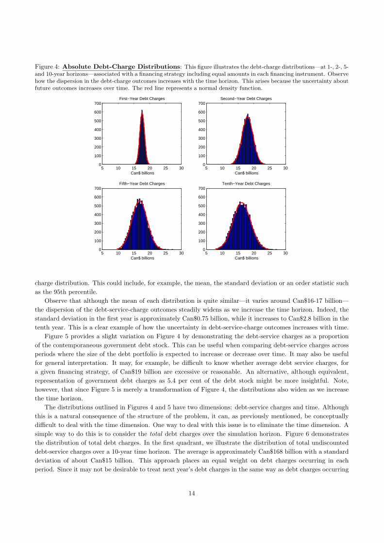
Figure 4: Absolute Debt-Charge Distributions: This figure illustrates the debt-charge distributions—at 1-, 2-, 5-and 10-year horizons—associated with a financing strategy including equal amounts in each financing instrument. Observehow the dispersion in the debt-charge outcomes increases with the time horizon. This arises because the uncertainty aboutfuture outcomes increases over time. The red line represents a normal density function.

5 10 15 20 25 300

100

200

300

400

500

600

700First−Year Debt Charges

Can$ billions5 10 15 20 25 30

0

100

200

300

400

500

600

700Second−Year Debt Charges

Can$ billions

5 10 15 20 25 300

100

200

300

400

500

600

700Fifth−Year Debt Charges

Can$ billions5 10 15 20 25 30

0

100

200

300

400

500

600

700Tenth−Year Debt Charges

Can$ billions

charge distribution. This could include, for example, the mean, the standard deviation or an order statistic suchas the 95th percentile.

Observe that although the mean of each distribution is quite similar—it varies around Can$16-17 billion—the dispersion of the debt-service-charge outcomes steadily widens as we increase the time horizon. Indeed, thestandard deviation in the first year is approximately Can$0.75 billion, while it increases to Can$2.8 billion in thetenth year. This is a clear example of how the uncertainty in debt-service-charge outcomes increases with time.

Figure 5 provides a slight variation on Figure 4 by demonstrating the debt-service charges as a proportionof the contemporaneous government debt stock. This can be useful when comparing debt-service charges acrossperiods where the size of the debt portfolio is expected to increase or decrease over time. It may also be usefulfor general interpretation. It may, for example, be difficult to know whether average debt service charges, fora given financing strategy, of Can$19 billion are excessive or reasonable. An alternative, although equivalent,representation of government debt charges as 5.4 per cent of the debt stock might be more insightful. Note,however, that since Figure 5 is merely a transformation of Figure 4, the distributions also widen as we increasethe time horizon.

The distributions outlined in Figures 4 and 5 have two dimensions: debt-service charges and time. Althoughthis is a natural consequence of the structure of the problem, it can, as previously mentioned, be conceptuallydifficult to deal with the time dimension. One way to deal with this issue is to eliminate the time dimension. Asimple way to do this is to consider the total debt charges over the simulation horizon. Figure 6 demonstratesthe distribution of total debt charges. In the first quadrant, we illustrate the distribution of total undiscounteddebt-service charges over a 10-year time horizon. The average is approximately Can$168 billion with a standarddeviation of about Can$15 billion. This approach places an equal weight on debt charges occurring in eachperiod. Since it may not be desirable to treat next year’s debt charges in the same way as debt charges occurring

14

Figure 5: Relative Debt-Charge Distributions: This figure illustrates the relative debt-charge distributions—at1-, 2-, 5- and 10-year horizons—associated with a financing strategy including equal amounts in each financing instrument.In this case, the debt charges are represented as a percentage of the total debt stock at that point in time. Again, weobserve how the dispersion in the debt-charge outcomes increases with the time horizon.

2 4 6 80

100

200

300

400

500

600

700First−Year Debt Charges

Per cent2 4 6 8

0

100

200

300

400

500

600

700Second−Year Debt Charges

Per cent

2 4 6 80

100

200

300

400

500

600

700Fifth−Year Debt Charges

Per cent2 4 6 8

0

100

200

300

400

500

600

700Tenth−Year Debt Charges

Per cent

10 years from now, we may wish to apply a discount factor to future debt-service charges. The complexity ofdiscounting cash flows, however, stems from the selection of the discount factor. Indeed, the remaining quadrantsof Figure 6 demonstrate the distribution of total discounted debt-service charges using flat 3 per cent, 5 per centand 7 per cent discount rates, respectively.

The discounting of future cash flows has two consequences. First, it reduces the absolute value of the totalgovernment debt charges by reducing the weight on future debt-service charges. Second, it leads to a decreasein the variance of the total debt-charge distributions. The undiscounted total debt charges have a standarddeviation of approximately Can$15 billion, while the total debt charges discounted at 7 per cent have a standarddeviation of slightly less than Can$10 billion. The reason is that, reducing the weight on the more volatilefuture debt charges, we actually decrease overall volatility. Clearly, selecting a discount factor is important whenconsidering total debt charges.27

The mean and standard deviation of the debt-charge distributions outlined in Figures 4 to 6 provide areasonable description of the normal cost and risk characteristics of a financing strategy. Debt managers are alsointerested in extreme outcomes; consequently, it makes sense to examine the tails of the previously illustrateddistributions. Figure 7 outlines a number of different flavours of CaR. The first quadrant plots the 10,000debt-charge sample paths from the stochastic simulation.

Absolute CaR is the worst-case expected debt-service charge with a certain degree of probability. Anotherway to think of absolute CaR is as a percentile measure; the 95 per cent CaR states that 95 per cent of the time,the government will not pay more than this amount in debt-service charges. The second quadrant of Figure 7provides a summary of the absolute CaR for 90 per cent, 95 per cent and 99 per cent probabilities, respectively.

27One could argue, of course, that, because of its arbitrary nature, we should forego the discounting of cash flows and merely

consider the simple sum.

15

Figure 6: Total Debt-Charge Distributions: This figure illustrates the total debt-charge distributions associatedwith a financing strategy including equal amounts in each financing instrument. We provide the distribution of a simplesum of debt charges over the 10-year simulation horizon as well as the distribution of summed and discounted debt chargesfor alternative discount factors.

100 150 2000

100

200

300

400

500

600Undiscounted

Can$ billions100 150 200

0

100

200

300

400

500

6003% Discount Factor

Can$ billions

100 150 2000

100

200

300

400

500

6005% Discount Factor

Can$ billions100 150 200

0

100

200

300

400

500

6007% Discount Factor

Can$ billions

Clearly, the higher the associated probability, the larger the CaR value. This is because we are moving furtherout the right tail of the distribution.

Relative CaR is simply the difference between absolute CaR and the mean of the distribution. The idea hereis that, if one uses the mean of the debt-charge distribution for planning, then relative CaR tells you that with,say, 95 per cent probability, one’s worst-case outcome will not exceed one’s planned outcome by more than thisamount. If one’s objective is to minimize budgetary shocks, such a measure could be quite useful in budgetaryplanning.

Conversely, tail CaR states how bad things can go, if they go bad. More specifically, a 95 per cent tail CaRstates the average debt charges assuming that debt charges are greater than or equal to the 95th percentile.In other words, this is the average debt charge in the tail of the distribution. This measure is useful when thedistribution has a small probability of extremely negative outcomes.28 Both relative and tail CaR are illustratedin Figure 7 for 90 per cent, 95 per cent and 99 per cent probabilities, respectively.

As noted earlier, there are potential advantages associated with defining risk in terms of budgetary out-comes in addition to government debt-service charges. Figure 8 illustrates the unadjusted funding-requirementdistributions associated with the first, second, fifth and tenth year of the stochastic simulation. This is a funding-requirement analogue of the debt-charge distributions outlined in Figure 4. The unadjusted funding requirementrepresents the size of the government’s deficit or surplus position before the application of the model’s fiscalrule.29

We observe that the mean funding requirement, across all periods, is approximately zero. We also observethat the standard deviation of the government’s funding requirement increases over time, albeit more slowly

28Statisticians refer to such distributions as fat-tailed or leptokurtotic.29A fiscal rule defines how the government reacts to deviations from expected fiscal positions.

16

Figure 7: Flavours of Cost-at-Risk: This figure illustrates the evolution of debt charges as well as absolute, relativeand tail cost-at-risk for a financing strategy consisting of equal weights in each financing instrument.

2 4 6 8 10

10

15

20

25

Debt−Charge Paths

Time (yrs.)

Ca

n$

bill

ion

s

2 4 6 8 10

19

19.5

20

20.5

21

21.5

22

22.5

Time (yrs.)

Ca

n$

bill

ion

s

Absolute CaR

90%

95%

99%

2 4 6 8 101

2

3

4

5

6

Time (yrs.)

Ca

n$

bill

ion

s

Relative CaR

90%

95%

99%

2 4 6 8 1019

20

21

22

23

Time (yrs.)

Ca

n$

bill

ion

s

Tail CaR

90%

95%

99%

than the debt-service charges. Both of these observations are a consequence of the specific parameterization ofthe funding-requirement process.

What is more important to draw from Figure 8 is the fact that, armed with these funding-requirementdistributions, we can proceed to compute the same mean, standard deviation and percentile measures in thesame manner as with the debt-service-charge distributions. We could, for example, construct a 95 per centbudget-at-risk measure that would describe, with 95 per cent probability, the worst-case budgetary outcomethat the government could experience in a given period for a particular financing strategy.30 Such a risk measurecould be quite useful in comparing the relative advantages and disadvantages of various financing strategies.

Table 1: Conditional Volatility: This table provides—in the context of the equally weighted financing strategy with10,000 simulations—the conditional volatility of the government debt charges and the government’s funding requirement,which we treat as a proxy for the government’s surplus/deficit position. Chapter 6 describes in greater detail how thegovernment’s fiscal position is determined.

Debt Quantity Conditional VolatilityDebt charges 1.73

Funding Requirements 2.92

The next set of risk measures relates to the previously discussed notion of conditionality. The conditional debtvolatility is computed as the standard deviation of the residuals of a regression of debt charges in period t runagainst debt charges from period t−1.31 This is a simple statistical technique for conditioning the debt charges in

30We can also compute interesting measures such as the probability that the government has a deficit of less than 1 billion dollars

in a given period.31More specifically, we run a simple first-order autoregression of the form yt = α + βyt−1 + εt. The actual regression equation,

17

Figure 8: Unadjusted Funding-Requirement Distributions: This figure illustrates the unadjusted funding-requirement distributions—at 1-, 2-, 5- and 10-year horizons—associated with a financing strategy with equal amounts ineach financing instrument. The unadjusted funding requirement represents the size of the government’s deficit or surplusposition before the application of the fiscal rule that (partially) offsets deviations from the expected deficit or surplusposition. Again, we observe how the funding-requirement outcomes increase with the time horizon.

−10 −5 0 5 100

200

400

600

800First−Year Funding Requirement

Can$ billions−10 −5 0 5 10

0

200

400

600

800Second−Year Funding Requirement

Can$ billions

−10 −5 0 5 100

200

400

600

800Fifth−Year Funding Requirement

Can$ billions−10 −5 0 5 10

0

200

400

600

800Tenth−Year Funding Requirement

Can$ billions

the current period on the previous period’s debt charges. The standard deviation of the regression errors capturesthe residual uncertainty in this relationship; i.e., the volatility that is left when one conditions on the currentstate of the world. This residual uncertainty is another potential dimension of risk to consider in comparingfinancing strategies. Moreover, by providing a single value, it essentially eliminates the time dimension.

Table 1 illustrates the conditional volatility of debt charges of Can$1.73 billion. What does this mean? Itmeans that, even when one takes into account the current debt charges, the standard deviation of the nextperiod’s debt charges is Can$1.73 billion. In other words, the residual debt-charge uncertainty over a 1-yearperiod, when taking into account the previous year’s outcomes, is Can$1.73 billion. This, of course, appliesacross all periods in the stochastic simulation.

The conditional volatility of the government’s funding requirement from Figure 8 is Can$2.92 billion. Again,this is residual budgetary uncertainty taking into account current conditions—which we can consider a measure ofthe fiscal uncertainty being faced. A government may wish, depending on its relative expense, to consider financ-ing strategies with slightly higher debt-service costs that act to simultaneously lower the conditional volatilityassociated with the funding requirement.

Next we consdier rollover risk. For single-day maturity risk, one intuitively understands that the more daysin a year that have bonds maturing, the lower the amount that matures on any given day. More specifically,doubling the number of maturity dates will halve the average amount maturing on any given day.32 Again,intuitively, one understands that as the term to maturity of a debt instrument increases, the amount rolling over

however, is stacked so as to incorporate all of the simulation outcomes. The conditional volatility is then estimated asq

1T−2

PTt=1 ε2t .

32Of course, in practice, maturing amounts will not be spread evenly, but the amount maturing on any single day will decrease

significantly.

18

Figure 9: Yearly Rollover Amounts: This figure illustrates the percentage of the debt that would, on average,rollover every year if all debt was issued at the tenor on the horizontal axis. For example, 3-month bills must be re-financed four times per year, so their annual rollover percentage is 400 per cent.

0 5 10 15 20 25 300

50

100

150

200

250

300

350

400Yearly Percentage Rollover

Tenor (yrs.)

Per

cen

t

in a given time period decreases. Figure 9 illustrates this, with an obvious bend occurring in the graph in the 1-to 5-year area.

3.3 Conclusion

This chapter has provided a brief, non-technical, example-based overview of a wide range of alternative measuresof the cost and risk associated with a given financing strategy. Two principal ideas are addressed in this discussion.First, the government faces a variety of fundamental risk and cost trade-offs in selecting a financing strategy forits domestic debt portfolio. Based on these definitions, therefore, we can proceed to select a financing strategythat minimizes the cost of the portfolio subject to constraints on its risk. This is the fundamental lesson fromportfolio theory.

The second point is that both cost and risk have a variety of dimensions. Cost can be computed in absolute,relative, summed or discounted terms. Risk can be related to the dispersion of debt-service charges and/orfunding-requirement outcomes as well as to financing risk. Moreover, it can be considered on a period-by-periodbasis or across time using a notion of conditionality. Table 2 provides a brief summary of the various risk measuresintroduced during this discussion. The complexity of the risk and cost dimensions reflects, in part, the underlyingcomplexity of the debt manager’s challenge. For this reason, we should not consider the preceding discussionof risk and cost measures as exhaustive, but rather as some measures that can, and should, be considered indebt-strategy analysis.

19

Table 2: Risk and Cost Measures: This table attempts to organize the collection of suggested risk and cost mea-sures, described in the text, into a logical structure. The idea is to highlight the various dimensions of the debt manager’schallenge and a number of alternative measures for describing each dimension in a modelling context.

Principal SecondaryDimension Dimension

Measure

Annual perspective√

Absolute debt charges√Relative (percentage) debt chargesCost

Aggregate perspective√

Total (summed) undiscounted debt charges√Total (summed) discounted debt charges√Standard deviation of debt charges

Cost-related risk √Absolute, relative and tail cost-at-risk√Conditional debt-charge volatility√Standard deviation of budgetary outcomesRisk Budget-related risk √Absolute, relative and tail budget-at-risk√Conditional budgetary volatility√Refixing share of debtRefinancing risk √Daily and quarterly rollover√Maturity profile

20

4 Introducing Inflation-Linked Bonds

This chapter focuses on the implications of incorporating inflation-linked debt into the debt-strategy model.As of 31 March 2011, approximately 6 per cent (or about Can$30.8 billion in real terms, Can$37.7 billion

inflation adjusted) of the government’s marketable debt stock consisted of inflation-linked debt.33 Introduced in1991, RRBs have been issued regularly for almost 20 years.

The debt-strategy model is sufficiently flexible to consider the relative advantages and disadvantages of nom-inal and inflation-linked debt. This chapter provides an overview of the principal issues involved in introducinginflation-linked debt into the debt-strategy analysis.

The chapter is divided into three sections. We begin by performing a simple comparison of a single inflation-linked bond relative to a single nominal bond: the aim is to highlight some of the modelling issues that arise inthis context and to generalize them for consideration in the debt-strategy model. We then examine an illustrativeexample, in the context of the full-blown debt-strategy model, of alternative financing strategies with differentproportions of inflation-linked debt. Finally, we make some concluding remarks.

4.1 A simple example

There are a few subtleties involved in comparing nominal and inflation-linked bonds. Before beginning a compar-ison of different financing strategies involving various proportions of nominal and inflation-linked debt, therefore,it is useful to begin in a simpler setting. Let us consider two 30-year bonds: one nominal bond with a 4 per centcoupon, and an inflation-linked bond with a 2 per cent real coupon. Assume that inflation is constant throughtime at 2 per cent.

We begin our comparison of these two bonds by examining their relative debt charges. The nominal bond,of course, pays an equal amount in each period. A coupon of 4 per cent and a notional value of, say, Can$100leads to an annual payment of Can$4. The inflation-linked coupon bond payment, however, in nominal terms,increases at the inflation rate of 2 per cent per year. The top-left quadrant of Figure 10 demonstrates theserelative debt charges. Observe that the nominal debt charges dominate their inflation-linked counterparts forevery period throughout the 30-year tenor of the bonds.

The principal payment of an inflation-linked bond, however, is adjusted upward for the accumulated inflationover its life. At 2 per cent inflation, therefore, the final principal payment of the inflation-linked bond would beCan$181.14. Clearly, this is a cost to the government and must be considered. In other words, an examinationof only the inflation-linked coupon, without inclusion of the principal compensation, would distort the analysis.When we compute and accrue the compounded 2 per cent growth in the inflation-linked principal, we generatean increasing annual cost for the government. The top-right quadrant of Figure 10 illustrates the sum of theinflation-linked coupon and principal uplift relative to the nominal bond’s debt charges. Observe that in thiscase, the inflation-linked debt charges dominate the nominal debt charges over the 30-year horizon.

There is, however, more to the story. The accrual of the inflation-linked principal uplift is necessary, but wecannot lose sight of the fact that it is a non-cash expense. The actual payment of the principal uplift occursat maturity. Conceptually, therefore, we can consider these non-cash expenses as a type of sinking fund. Theseexpenses must be offset by the interest compensation that could have been earned on these funds. In other words,even if no cash payment is made, by realizing a non-cash expense many periods before it is actually required, itis necessary to discount this cash flow to its present value. Not making this adjustment will lead one to concludethat inflation-linked bonds are more expensive relative to their nominal equivalent.

The bottom-left quadrant of Figure 10 illustrates the annual accrual of the 2 per cent compounded increasein the principal of the inflation-linked bond. It also illustrates the return—assumed to be 4 per cent—on thenon-cash accruals. We term this the offset. Combining the accrual and offset generates the net debt charges

33In Canada, as described earlier in the paper, inflation-linked debt is known as Real Return Bonds (RRBs). RRBs are long-term

instruments, with issuance beginning at 30+ years to maturity.

21

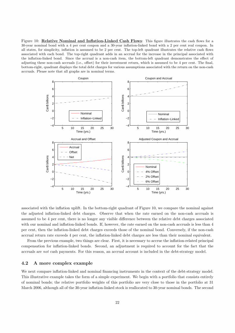
Figure 10: Relative Nominal and Inflation-Linked Cash Flows: This figure illustrates the cash flows for a30-year nominal bond with a 4 per cent coupon and a 30-year inflation-linked bond with a 2 per cent real coupon. Inall states, for simplicity, inflation is assumed to be 2 per cent. The top-left quadrant illustrates the relative cash flowsassociated with each bond. The top-right quadrant adds in an accrual for the increase in the principal associated withthe inflation-linked bond. Since the accrual is a non-cash item, the bottom-left quadrant demonstrates the effect ofadjusting these non-cash accruals (i.e., offset) for their investment return, which is assumed to be 4 per cent. The final,bottom-right, quadrant displays the total debt charges for various assumptions associated with the return on the non-cashaccruals. Please note that all graphs are in nominal terms.

5 10 15 20 25 30−4

−2

0

2

4

6

8

Time (yrs.)

Can

$ bi

llion

s

Coupon

5 10 15 20 25 30−4

−2

0

2

4

6

8

Time (yrs.)

Can

$ bi

llion

s

Coupon and Accrual

5 10 15 20 25 30−4

−2

0

2

4

6

8

Time (yrs.)

Can

$ bi

llion

s

Accrual and Offset

5 10 15 20 25 30−4

−2

0

2

4

6

8

Time (yrs.)

Can

$ bi

llion

s

Adjusted Coupon and Accrual

Nominal

Inflation−LinkedNominal

Inflation−Linked

Accrual

Offset

Net

Nominal

4% Offset

2% Offset

6% Offset

associated with the inflation uplift. In the bottom-right quadrant of Figure 10, we compare the nominal againstthe adjusted inflation-linked debt charges. Observe that when the rate earned on the non-cash accruals isassumed to be 4 per cent, there is no longer any visible difference between the relative debt charges associatedwith our nominal and inflation-linked bonds. If, however, the rate earned on the non-cash accruals is less than 4per cent, then the inflation-linked debt charges exceeds those of the nominal bond. Conversely, if the non-cashaccrual return rate exceeds 4 per cent, the inflation-linked debt charges are less than their nominal equivalent.

From the previous example, two things are clear. First, it is necessary to accrue the inflation-related principalcompensation for inflation-linked bonds. Second, an adjustment is required to account for the fact that theaccruals are not cash payments. For this reason, an accrual account is included in the debt-strategy model.

4.2 A more complex example

We next compare inflation-linked and nominal financing instruments in the context of the debt-strategy model.This illustrative example takes the form of a simple experiment. We begin with a portfolio that consists entirelyof nominal bonds; the relative portfolio weights of this portfolio are very close to those in the portfolio at 31March 2006, although all of the 30-year inflation-linked stock is reallocated to 30-year nominal bonds. The second

22

financing strategy involves a transfer of one-half of 30-year nominal bond stock into 30-year inflation-linked debt.The third financing strategy replaces all 30-year nominal debt with inflation-linked bonds of equivalent tenor.These three financing strategies are summarized in Table 3.

Table 3: Financing Strategies: This table outlines three alternative financing strategies involving nominal andinflation-linked bonds of alternative tenors.

Financing StrategiesDebt Type Tenor0% Real 17.5% Real 35% Real

3 month 19% 19% 19%6 month 6% 6% 6%1 year 6% 6% 6%2 year 5% 5% 5%5 year 6% 6% 6%10 year 22% 22% 22%

Nominal

30 year 35% 17% 0%Real 30 year 0% 17% 35%

Clearly, such abrupt changes in the government’s debt portfolio cannot be achieved in a short period oftime. We can think of this exercise, therefore, as a thought experiment involving the comparison of threeportfolios—and their associated financing strategies—that differ only in their relative proportions of nominaland inflation-linked debt. By varying the proportions of 30-year nominal debt and inflation-linked securitiessharing the same tenors, the basic maturity structure of the portfolio is preserved. This permits, in our view, afair characterization of the risk and cost differences between portfolios with an increasing share of inflation-linkeddebt.

We compare these three alternative financing strategies using 10,000 randomly generated realizations ofoutput, inflation, the monetary policy rate and the term structure of interest rates. The average financing rates,and their associated standard deviations, are presented in Table 4. These financing rates are essentially thecoupon rates associated with issuing inflation-linked or nominal bonds at a price of par.

Table 4 shows that the average 30-year nominal par coupon is 5.27 per cent. This compares to a mean realcoupon of 3.07 per cent for the 30-year inflation-linked bonds. If we adjust these real coupons for the averageinflation of 1.98 per cent, we arrive at an approximate average cost for the 30-year inflation-bonds of 5.05 percent. This is approximately 20 basis points less than the corresponding coupon associated with 30-year nominalborrowing. Based on the analysis in the previous section, therefore, we should expect to observe only slight costdifferences for the financing strategies that include more inflation-linked debt.34

Figure 11, in fact, illustrates the annual debt charges for each of three financing strategies across the 10-yearsimulation horizon in Canadian-dollar and percentage terms. Observe that the financing strategy with the largestproportion of inflation-linked debt demonstrates slightly higher expected debt charges; this effect is related to theissuance-penalty function described in Chapter 9. The 17.5 per cent allocation to inflation-linked debt, however,leads to, relative to the nominal-debt-dominated strategy, lower debt-service charges on the order of a few basispoints. We also observe that the two financing strategies with inflation-linked debt exhibit lower debt-chargestandard deviation across almost all periods in the simulation horizon.

Figure 12 demonstrates how the greater dispersion of debt-charge outcomes in the nominal-bond-based fi-nancing strategy translates into slightly higher relative cost-at-risk values. This is particularly true—given thehigher expected debt charges of the 35 per cent inflation-linked financing strategy—on a relative basis. Thisappears to be a diversification benefit. Real par coupon rates are slightly more variable than nominal parcoupon rates and the entire inflation-indexed portfolio is repriced every period, while only the 30-year nominal

34As well, the calculation does not include an issuance penalty. The issuance-penalty function is described in Chapter 9.

23

Table 4: Financing Rates: This table outlines mean and standard deviation of the randomly generated par couponsassociated with nominal and inflation-linked debt in the model. It also includes the mean and standard deviation ofrealized-inflation outcomes stemming from the stochastic model. The historical data period used is 1994 to 2007.

Financing CostDebt Type TenorMean Coupon Standard Deviation

3 month 3.85 1.292 year 4.26 1.1510 year 5.04 1.10Nominal

30 year 5.27 1.0810 year 2.12 0.78Real30 year 3.07 1.10

Inflation Annualized 1.98 0.26

debt coming to maturity, and any issuance to cover the financial requirement, is repriced in a given quarter.35

Therefore, inflation-indexed bonds alone are more variable, but they appear to contribute to lower variability indebt charges in a portfolio with nominal bonds.

Figure 12 also illustrates the budget-at-risk (BaR) values for our three financing strategies. Similar to thedebt-charge setting, the financing strategies with inflation-linked debt appear to be less risky than the 35 percent nominal 30-year portfolio. These modest differences apply on both an absolute and a relative basis. Thereason for these phenomena appear to be found in the bottom-left quadrant of Figure 13, which describes theaverage correlation between the government’s primary balance and the debt-service charges. As we increase theproportion of inflation-linked debt, the magnitude of this correlation increases. The variance of the government’sbudget balance is equal to the sum of the variance of the primary balance and the debt charges less twice theircovariance.36 As such, the larger the covariance between the primary balance and debt charges, ceteris paribus,the lower the variance of the government’s budgetary balance. We suggest that the larger positive correlationbetween the debt charges and the primary balance, for the financing strategies containing 30-year inflation-linkeddebt, is responsible for the superior BaR numbers, compared to the financing strategy containing only 30-yearnominal bonds, in Figure 12.37

Why do we observe a higher correlation between the primary balance and debt charges as we increase theproportion of inflation-linked debt in the portfolio? We believe that the answer relates to the structure of theprimary balance and the associated debt charges. The debt charges represent a weighted average of currentand past financing decisions. A financing strategy dominated by long-term issuance places more weight on pastfinancing decisions (and consequently past interest and inflation rates), whereas a short-term financing strategyleads to a larger weight on current interest and inflation rates. The primary balance, conversely, dependsprincipally on contemporaneous changes in output and inflation. The three financing strategies analyzed in thischapter have, by their very construction, the same amount of short- and long-term debt. As a consequence, thedifferences in correlation do not directly depend on the relative weights of interest rates through time.

The difference relates, however, to the composition of the debt charges. With a financing strategy involvingonly nominal bonds, the debt charges consist entirely of coupon payments determined either in the past orthe current period. When we add inflation-linked bonds, the debt charges consist of nominal and real couponsdetermined in current and past periods plus the uplift in the inflation-linked principal, which is a function of

35In fact, a 100 per cent portfolio of 30-year RRBs has a conditional debt-charge volatility of around 2, versus about 0.5 for a 100

per cent portfolio of 30-year nominal bonds.36The fiscal rule implemented in the model is described in Chapter 6.37Clearly, there is some offset in the other parts of budgetary volatility. The debt charges of the 35 per cent inflation-indexed

portfolio have a higher correlation with the primary balance, but similar budgetary-risk outcomes, compared to the 17.5 per cent

inflation-indexed portfolio.

24

Figure 11: Mean and Standard Deviation Government Debt Charges: This figure illustrates the expecteddebt charges and standard deviation associated with three alternative financing strategies: no inflation-linked bonds, thereplacement of one-half of the nominal 30-year nominal bonds with inflation-linked bonds, and the entire replacement of30-year nominal with inflation-linked bonds. The mean debt charges are presented, for each year in the 10-year simulationhorizon, in absolute and relative terms. We also present the standard deviation of these debt charges.

2 4 6 8 10

17.8

17.9

18

18.1

18.2

18.3

18.4

18.5

Time (yrs.)

Can

$ bi

llion

s

Mean Debt Charges

2 4 6 8 10

4.6

4.65

4.7

4.75

4.8

4.85

Time (yrs.)P

er c

ent

Percentage Debt Charges

1 2 3 4 5 6 7 8 9 10

1

1.5

2

Time (yrs.)

Can

$ bi

llion

s

Standard Debt−Charge Deviation

0% RRBs

17.5% RRBs

35% RRBs

contemporaneous inflation. While these three elements generally move together, they are not perfectly correlated.As such, movements in the contemporaneous component of debt charges for a financing strategy that includesinflation-linked bonds are more complex than for an equivalent strategy that consists only of nominal bonds.Moreover, the inflation-linked principal compensation has a much larger contemporaneous component than itsnominal equivalent. We argue that the addition of the relatively more contemporaneous component to theinflation-linked debt charges acts to modestly increase its overall correlation with the primary balance.

We performed some sensitivity analysis around these results in the form of using different starting points forthe simulation of the random outcomes. The reported results use interest rates, inflation, output and monetaryconditions from 2007 as the starting point. We also considered using the long-term mean values from theestimation and the average historical values as our starting points. The consequence of using different startingvalues is alternative paths for interest rate and macroeconomic variables. Our sensitivity analysis indicates that,while the general pattern of the results remains the same, the magnitude of the differences in the financingstrategies depends on the starting point for the simulation.

Analysis has been performed on the correlation structure of debt charges using 100 per cent portfolios in eachinstrument. It has shown that inflation-indexed 30-year bonds have extremely low correlations with nominalinstruments, relative to nominal instruments’ correlations with each other.38 This provides further evidence of

38It is unclear how much of this relates to incorporating the present value of principal uplifts in costs as they occur. As discussed,

in reality this is the incurrence of a cost, but not the payment of one. It is therefore, within the model, a non-cash item in the

25

Figure 12: Cost- and Budget-at-Risk Measures: This figure again illustrates various risk measures associatedwith three alternative financing strategies: no inflation-linked bonds, the replacement of one-half of the 30-year nominalbonds with inflation-linked bonds, and the entire replacement of 30-year nominal with inflation-linked bonds. The 95 percent absolute cost-at-risk (CaR) and budget-at-risk (BaR)—over the 10-year simulation horizon–is presented for each ofthe strategies. The 95 per cent relative CaR and BaR are also computed.

2 4 6 8 10

20

20.5

21

21.5

22

Time (yrs.)

Can

$ bi

llion

s

Absolute CaR

2 4 6 8 10

1.5

2

2.5

3

3.5

4

Time (yrs.)

Can

$ bi

llion

s

Relative CaR

2 4 6 8 10

−1.5

−1

−0.5

0

0.5

Time (yrs.)

Can

$ bi

llion

s

Absolute BaR

2 4 6 8 10

2

2.5

3

3.5

Time (yrs.)

Can

$ bi

llion

sRelative BaR

0% RRBs

17.5% RRBs

35% RRBs

the diversification benefit of holding some inflation-indexed debt in the government’s debt portfolio.As a final point, it is important to highlight that the above thought experiment and discussion centre on the

characteristics of a portfolio that includes inflation-indexed bonds. However, caution is warranted. It does notdescribe their role in an optimal portfolio at a given risk level, or at a desired cost-risk trade-off.39

4.3 Conclusion

This chapter has introduced inflation-linked bonds into the analysis of the government’s debt strategy. A thoughtexperiment involving alternative financing strategies with different proportions of inflation-linked debt has led tothree preliminary conclusions. First, using stochastic outcomes estimated to Canadian data from 1994 to 2007implies relatively modest differences in the expected cost of these financing strategies. Second, the volatility ofthe debt charges appears to be somewhat lower for financing strategies with inflation-linked debt; the reasonappears to be a diversification benefit from having both nominal and inflation-indexed debt in the portfolio. Thisresult also extends to budgetary volatility. In that context, it seems to be also driven by the positive correlationbetween debt charges and the primary balance among financing strategies with inflation-indexed bonds. Themodel is capable of adding shorter inflation-indexed maturities, and evaluating instruments that link paymentsto other economic indicators.

budget.39Optimization is discussed in Chapter 5.

26

Figure 13: Debt Stock and Funding Measures: This figure again illustrates various debt-stock and funding-requirement measures associated with three alternative financing strategies: no inflation-linked bonds, the replacementof one half of the 30-year nominal bonds with inflation-linked bonds, and the entire replacement of 30-year nominalwith inflation-linked bonds. For each financing strategy, the expected debt stock, its standard deviation, the correlationbetween debt charges and the primary balance, and finally the expected funding requirement are presented.

2 4 6 8 10370

375

380

385

390

395

Time (yrs.)

Can

$ bi

llion

s

Expected Debt Stock

2 4 6 8 10

2

3

4

5

Time (yrs.)

Can

$ bi

llion

s

Debt Stock Standard Deviation

2 4 6 8 10

0.2

0.3

0.4

0.5

0.6

Time (yrs.)

Cor

rela

tion

coef

ficie

nt

Primary Balance − Debt Charge Correlation

2 4 6 8 10−3.5

−3

−2.5

Time (yrs.)

Can

$ bi

llion

s

Funding requirement

0% RRBs

17.5% RRBs

35% RRBs

27

5 The Optimization Module

This chapter explores the optimization tool developed specifically for application to the debt-strategy problem.As we have seen in the preceding chapters, stochastic-simulation models provide substantial information ona given financing strategy. Indeed, they permit the detailed comparison of two or more alternative financingstrategies on a wide variety of dimensions. One shortcoming of this approach, when we rely only on the simulationengine, is that the model does not provide any insight into the optimal debt strategy that should be followedby the government. That is, we can compare two or more strategies in great detail, but there is nothing to saythat any of the considered strategies is optimal. This is not to say, however, that stochastic-simulation modelsare incapable of providing insight into a government’s optimal debt strategy. More structure is required. Thischapter discusses this structure in the form of the recently developed optimization module that was built tosupplement our stochastic-simulation model.

Two substantial challenges must be overcome to use stochastic-simulation models in an optimization context.First, one must handle the difficulties associated with optimizing in a computationally expensive setting. This isessentially a mathematical challenge that will not—beyond a brief high-level description—be addressed in thispaper.40 The second challenge is that we require precision about what exactly is meant by the idea of an optimaldebt strategy. This is far from straightforward. Even experienced debt managers can disagree on the specificrisk constraints that should apply to the government’s debt strategy. Even in the event of an agreement on thetype of constraint, there may not be consensus on the level of the constraint.

Irrespective of the complexities of explicitly describing the government’s objective function, the disciplineof characterizing one’s objective function is, to our mind, quite valuable. Moreover, examining the sensitivityof the portfolio to different types of constraints and different constraint levels can be very illuminating. Thesecond challenge, therefore, forms the backbone of this discussion paper. It should, however, be stressed thatthis paper does not seek to suggest the optimal debt strategy for the government. Instead, these are illustrativeand exploratory results intended to provide a sample of what can be done with the optimization tool.

A note of caution should be given regarding the results shown. They are from 2007 and are for illustrativepurposes only, to show the types of analysis that can be accomplished with the model.41

The chapter is organized into two parts. In the first part, we engage in a high-level discussion of the opti-mization algorithm to motivate and build intuition about the tool. The second part considers the minimizationof debt charges subject to a reasonably wide range of constraints. We consider two broadly defined constraintcategories. In the first group, the constraints relate to notions of interest rate and budgetary risk. In the secondgroup, the constraints are related to portfolio-summary measures (i.e., average term to maturity and the refixingshare of debt) and treasury bill and bond issuance. For each constraint, we examine how the portfolio weightsevolve for different constraint levels, as well as the trade-off between expected cost and the constraint. Thecurrent portfolio is also indicated to provide some context to our analysis.

5.1 Background

Optimizing in a stochastic-simulation setting is a high-dimensional, non-linear and computationally intensivemathematical problem. It is the computational expense that is the real challenge. The reason is simple—simulation is a powerful statistical technique, but it is slow. The evaluation of a single financing strategy with10,000 randomly generated outcomes can require more than one half hour of computation. Most non-linearoptimization algorithms work iteratively and require repeated evaluation of one’s objective function—in ourcase, this means repeatedly rerunning the simulation. Depending on the number of instruments, this can meanliterally thousands of simulations. Put simply, solving a single optimization problem can take weeks. This isunacceptably slow and makes direct optimization impractical.

40A detailed discussion of the mathematics of the optimization algorithm is provided in Bolder and Rubin (2007).41Some differences from today are the Can$400 billion debt stock and the absence of the recently reintroduced 3-year maturity.

28

If there was universal consensus on the form of the government’s debt-strategy objective function, thenwe might be content to merely let an optimizer run over a number of weeks to obtain the final response. This,however, is not the case. We would like to run numerous optimizations with alternative constraints and constraintlevels. We also want to tweak the model assumptions and understand the sensitivity of the optimum to thesechanges. Each optimization, and the corresponding comparison with our intuition, has the potential to help uslearn more about the debt manager’s challenge. In short, we desire a fast and efficient optimization algorithm.

Fortunately, recent work has helped lead to the development of an optimization module for solving thismathematical challenge. The basic idea behind the optimization module is quite simple. First, we cannot, byvirtue of the incredible computational expense, perform the optimization directly on the simulation engine. As aconsequence, we instead approximate a given debt-strategy objective function. We then proceed to perform theoptimization algorithm on this approximation. In other words, we run a fixed number of simulations—say, one ortwo thousand—for different financing strategies. We can consider this work as a form of overhead, which generallyrequires a few days of computation. Using this fixed number of simulations, we construct an approximation of thesimulation for any financing strategy. Any feature of the simulation can thus be approximated in an extremelyrapid manner. Once we have incurred the overhead, a given optimization can be performed in a number ofseconds.

This is the basic idea behind the optimization engine. Clearly, there is a substantial amount of mathematicaldetail behind this component. The interested reader can consult the references for more discussion, although itis not necessary for the use of the optimization policy tool.

5.2 Alternative optimization constraints

There are a virually limitless number of possible specifications for the government’s debt-management objectivefunction. Some direction, therefore, is required. Once again, it makes good sense to consider the publicly statedobjectives of the Canadian government with respect to this portfolio:

The main debt-management objective is to raise stable, low-cost funding to meet the operational needsof the government. An associated objective is to maintain a well-functioning market for governmentsecurities.

In Chapter 3, we examined a number of approaches for translating these notions of low cost and stability intomore formal risk and cost measures.

In this analysis, we use the average annual debt charges as a percentage of the total debt stock over the10-year simulation horizon as our measure of cost. The advantage of this approach is that it avoids the need todiscount the debt stock and is relatively robust to different debt-stock levels. It is also attractive because of itsrelative ease of computation.42

The actual optimization problem used to generate the results in this section is quite straightforward. Weassume that the government wishes to minimize the percentage cost of the debt over the next 10 years—thisis our definition of low cost—subject to a single constraint. We vary the choice of constraint and its leveland examine the results. Each of these constraints can loosely be considered as an alternative definition ofstability. A verbal description of the optimization problem, therefore, following from the guidance provided byour debt-management guidelines, would look something like,

minPortfolioweights

Expected Debt Cost, (1)

subject to:

Risk ≤ Predetermined Level.

42It should be stressed, however, that the following results are generally robust to the choice of cost measure and where relevant,

and within a reasonable range, to the discount factor.

29

Risk, of course, is the mirror image of stability. We can either require that the risk be less than some pre-determined level, or demand that the stability be greater than another predetermined level.

Let us examine the application of this notion to our debt-strategy model. We consider 2,000 alternative financ-ing strategies—with 10,000 random realizations of our stochastic model—including eight financing instruments.The data used to estimate the stochastic model run from 1994 to February 2007.43 The financing strategiesinclude 3-, 6- and 12-month treasury bills; 2-, 5-, 10- and 30-year nominal bonds; and 30-year inflation-linkedbonds. In each case, we assume an annual debt paydown target of Can$3 billion and follow the description ofthe government’s fiscal situation provided in Chapter 6. These 2,000 financing strategies serve as the dataset fortraining, or fitting, our approximation functions. Once the approximation functions are trained, we can considera wide range of possible government objective functions.

Figure 14: Risk-Constrained Optimizations: This figure illustrates how the optimal portfolio weights evolve fordifferent fixed risk-constraint values. In each case, the optimizer seeks to minimize the expected average percentagedebt charges over the 10-year simulation horizon. Each of the four graphs represents an alternative risk constraint. Thehorizontal axis represents alternative levels of the constraint. The first graph, for example, examines how the portfolioweights change as we increase the constraint on annual conditional debt-charge volatility from Can$500 million to Can$4billion. The other three graphs demonstrate the corresponding results by using conditional budgetary volatility, thefirst-year relative CaR and average quarterly rollover, respectively.

1 2 3 40

20

40

60

80

100Conditional Debt−Charge Volatility

Conditional Debt−Charge Volatility (Can$ billions)

Por

tfolio

wei

ght (

%)

3 3.5 40

20

40

60

80

100Conditional Budgetary Volatility

Conditional Budgetary Volatility (Can$ billions)

Por

tfolio

wei

ght (

%)

1 2 3 40

20

40

60

80

100First−Year Relative CaR

First−Year Relative CaR (Can$ billions)

Por

tfolio

wei

ght (

%)

50 100 150 200 250 3000

20

40

60

80

100Average Quarterly Rollover

Average Quarterly Rollover (Can$ billions)

Por

tfolio

wei

ght (

%)

RRB30y10y5y2y1y6m3m

43There are a variety of possible stochastic models from which we can choose. In this analysis we use the Diebold and Li (2003)

approach applied to the Nelson and Siegel (1987) model as described in Bolder (2006). We have forced the long-term inflationary

mean to be 2 per cent and the long-term output gap to be zero.

30

5.2.1 Risk constraints

Armed with these results, each of the four graphs in Figure 14 represents an alternative risk constraint. Thehorizontal axis represents alternative levels of the constraint, while the vertical axis denotes the portfolio weights.A specific example of the results found in Figure 14 would have the following form,44

minPortfolioweights

Expected Average Percentage Debt-Service Charges, (3)

subject to:

Conditional Cost Volatility ≤ Can$1 billion.

In words, the optimizer attempts to find the set of portfolio weights that provide the lowest possible totaldebt charges while simultaneously respecting the constraint of conditional debt-charge volatility less than Can$1billion.

We are not, however, restricted to merely constraining conditional debt-charge volatility to Can$1 billion; wecan examine a wide range of possible constraint levels. The top-left graphic in Figure 14, in fact, provides theoptimal financing strategies (i.e., portfolio weights) for conditional debt-charge volatility ranging from Can$500million to Can$4 billion. The easiest way to read these figures is to work from left to right on the horizontalaxis. At the lowest level of the conditional debt-charge volatility constraint (i.e., Can$500 million), the optimalportfolio weights involve about 23 per cent 30-year, 52 per cent 10-year, 15 per cent 5-year and 10 per cent2-year nominal bonds. As the conditional debt-charge volatility constraint relaxes, the 30- and 10-year bondsare replaced with 2-year bonds and treasury bills. Beyond a constraint of approximately Can$3.5 billion, theportfolio weights settle down at over 95 per cent treasury bills, with the majority allocated to 3- and 6-monthtenors, as well as a small allocation to 5-year bonds. Once the constraint no longer binds, we have the lowest-costportfolio, which is the same for all risk constraints.45

The changing portfolio weights in Figure 14 are interesting, but they do not tell us how much debt-servicecharges are reduced as the constraint is eased. This information is provided in Figure 15. We see, for example,in the top-left quadrant of Figure 15, that as the conditional debt-charge volatility constraint is eased—fromCan$500 million to Can$3 billion—the expected cost falls by approximately 100 basis points.46

The top-right quadrant of Figure 14 illustrates the conditional budgetary volatility. For lower levels of the riskconstraint, the optimal portfolio allocation involves a substantial proportion of inflation-linked debt, 10- and 30-year nominal debt, and treasury bills. As the risk constraint is relaxed, however, the optimal portfolio weightsshift to include significant proportions of 10-year bonds and treasury bills. Beyond approximately Can$3.75billion, however, the portfolio involves 5 per cent 5-year bonds with the remaining 95 per cent in treasury bills—the majority of this, about 60 per cent, is allocated to the 3-month treasury bill. Figure 15 shows that there isalso approximately 100 basis points of cost reduction as one eases the conditional budgetary volatility constraintfrom Can$2.7 to Can$3.75 billion.

44In mathematical notation, this problem is stated as follows,

minθ∈Θ

1

T

TXt=1

1

Ξt

· Ect− 1, t, θ, X(t, ω)

F0

, (2)

subject to:

σt− 1, t, θ, X(t, ω)

Ft−1

≤ δ.

where c denotes the debt-servicing charges over the interval [0, t] for fixed θ ∈ Θ and financing strategy ω ∈ Ω, X denotes the

discretized state variable vector, σ is the conditional debt-charge volatility, Ξt is the nominal value of the government debt stock at

time t, and δ is Can$1 billion.45This occurs when loosening the constraint leads to no change in the portfolio, and therefore no further cost reduction.46For a debt stock of Can$400 billion, this represents approximately Can$4 billion of annual cost reduction.

31

Figure 15: Expected Cost of Risk-Constrained Optimizations: This figure illustrates the optimal risk-costtrade-off for different fixed risk-constraint values. These results are described in Figure 14. The underlying figures illustratethe expected cost, as a percentage of the debt stock, for the optimal portfolios associated with each given constraint level.

1 2 3 44

4.2

4.4

4.6

4.8

5

Conditional Debt−Charge Volatility

Constraint (Can$ billions)

Exp

ecte

d co

st (

per

cent

)

3 3.5 44

4.2

4.4

4.6

4.8

5

Conditional Budgetary Volatility

Constraint (Can$ billions)

Exp

ecte

d co

st (

per

cent

)

1 2 3 44

4.2

4.4

4.6

4.8

5

First−Year Relative CaR

Constraint (Can$ billions)

Exp

ecte

d co

st (

per

cent

)

50 100 150 200 250 3004

4.2

4.4

4.6

4.8

5

5.2Average Quarterly Rollover

Constraint (Can$ billions)

Exp

ecte

d co

st (

per

cent

)

The bottom-left quadrant of Figure 14 involves the application of a constraint on the relative cost-at-risk(CaR) in the first year of the simulation. This constraint applies over the range Can$250 million to Can$4 billion.Once again, for tight constraint levels, the allocation is predominately composed of long-tenor nominal bondswith modest amounts of 2- and 5-year nominal bonds and zero treasury bill allocation. Beyond a constraintof approximately Can$2.5 billion, the optimal portfolio weights involve treasury bills and 2- and 5-year bonds.Figure 15 illustrates that there are approximately 100 basis points of cost reduction in easing the first-yearrelative CaR constraint from Can$250 million to Can$3 billion. Beyond this point, the constraint no longerbinds.

The bottom-right quadrant in Figure 14 describes the final constraint on the average quarterly rolloveramount. The constraint ranges from Can$10 billion to Can$300 billion. Not surprisingly, low-risk levels see largeallocations to 10-year, and to a lesser extent 30-year, bonds. As the constraint is loosened, there is a gradualincrease in the treasury bill allocation, starting with the 1-year treasury bill. Moreover, the cost of the portfolio,as evidenced in Figure 15, falls by about 100 basis points as we ease this constraint.

Figures 14 and 15 illustrate how the optimal portfolio weights and expected costs evolve for different riskconstraints at alternative constraint levels. While the results vary as one changes the constraint, there is a generaltrend toward an increase in the amount of longer-tenor instruments as one desires to reduce risk. Moreover, inall cases, this reduction in risk is accompanied by a commensurate increase in expected debt-service charges.

5.2.2 Adding more constraints

This section outlines the use of two additional constraints. The first one is having a minimum issuance amount(in terms of portfolio weight) for each maturity. This restricts the optimization to only those portfolios that

32

have a portfolio weight above each instrument’s constrained level.47 The second is a maximum average quarterlyrollover constraint. While a constraint on rollover was used earlier as the main risk constraint, it can also beadded to other optimizations to ensure that the level of rollover remains at an acceptable level. Both constraintscan be used at the same time, or each separately.48

Figure 16: Adding Issuance and Rollover Constraints: This figure compares how the optimal portfolio weightsand expected costs evolve when issuance and rollover constraints are added to the conditional debt-charge volatilityoptimization. The first three graphs show the optimal portfolio weights for the no additional constraints (same as thetop-left graph in Figure 14), issuance constrained, and issuance and Can$80 billion rollover constrained optimizations.In each case, the optimizer seeks to minimize the expected average percentage debt charges over the 10-year simulationhorizon. The final graph (bottom right) shows the expected costs for each of the three optimizations.

1 2 3 40

20

40

60

80

100No Additional Constraints (UC)

Conditional Debt−Charge Volatility (Can$ billions)

Po

rtfo

lio w

eig

ht

(%)

1 1.2 1.4 1.6 1.8 20

20

40

60

80

100Issuance Constrained (IC)

Conditional Debt−Charge Volatility (Can$ billions)

Po

rtfo

lio w

eig

ht

(%)

1 1.2 1.4 1.6 1.8 20

20

40

60

80

100Issuance and 80B Roll Constrained

Conditional Debt−Charge Volatility (Can$ billions)

Po

rtfo

lio w

eig

ht

(%)

1 2 3 44

4.2

4.4

4.6

4.8

5

Cost−Risk Tradeoffs

Conditional Debt−Charge Volatility (Can$ billions)

Exp

ect

ed

Co

st (

pe

rce

nt)

RRB

30y

10y

5y

2y

1y

6m

3m

IC+$80B RollICUC

There are several points to emphasize in Figure 16. First, the range of constraint levels is significantlyreduced (from Can$0.5 billion to Can$4 billion, to Can$1 billion to Can$2 billion) in the issuance-constrainedand issuance and rollover constrained (top-right and bottom-left) graphs. Debt-charge volatility cannot bereduced below Can$1 billion, likely because of forced issuance in treasury bills, and perhaps also due to forcedissuance in RRBs. The inability to increase debt-charge volatility beyond Can$2 billion appears mainly due tothe forced issuance in the 30-year nominal and 30-year RRB maturities (and, to a lesser extent, the 10-yearmaturity), which are either not present or present at a reduced level in the top-left graph with no additionalconstraints.49 The forced long-term issuance also contributes to higher expected cost, as can be seen from the

47This level will differ across instruments, and is updated regularly to reflect market conditions.48There are numerous combinations of constraints that could be used. For example, one could run an optimization with rollover

as the main risk constraint, with a maximum allowable value on conditional debt-charge volatility and/or conditional budgetary

volatility.49RRBs appear to have a high enough impact on debt-charge volatility to infringe on risk reduction, while also having a small

enough impact on debt-charge volatility to prevent reaching increasing risk levels.

33

fact that the red and green lines are above the blue line in the bottom-right graph. Clearly, imposing issuanceand rollover constraints is restrictive in terms of reachable conditional debt-charge volatility levels, and leads tohigher expected costs.

Second, the issuance constrained and issuance and rollover-constrained optimizations give the same results upto a conditional debt-charge volatility level of about Can$1.4 billion. This can be seen by the fact that the red andgreen lines overlap in the bottom-right graph in Figure 16. This occurs because the rollover constraint does notbind until the Can$1.4 billion constraint level. In other words, the issuance-constrained optimal portfolios untilthat point have an average quarterly rollover level under Can$80 billion, and so adding the rollover constrainthas no effect on them.

Third, in terms of portfolio allocation, the addition of the Can$80 billion rollover constraint causes a reductionin the 3-month treasury bill weight, starting at about a Can$1.4 billion conditional debt-charge volatility level,with it being replaced with 6-month and 1-year treasury bills.

5.2.3 Portfolio-summary measures and primary issuance constraints

This section examines constraints that are motivated by notions of portfolio composition and debt issuance.Practically, debt managers are interested not only in notions of risk stemming from the moments of debt-chargeand budgetary distributions. Constraints also arise in other forms. In particular, portfolio-summary measuresare of interest to debt managers for internal and external communication. We consider two common measures:the refixing share of debt and the average term to maturity (ATM).

A second example is primary issuance. A fundamental principal of debt management is that concentrationof issuance in specific market segments permits reduction of liquidity premia that creates a corresponding costsavings for debt issuers. To this end, it also makes sense to consider the application of constraints to primaryissuance. Again, we consider two potential measures: average biweekly treasury bill issuance and average annualbond issuance.

Figure 17 illustrates the portfolio weights—in a manner analogous to Figure 14—for these four alternativeportfolio-summary and issuance constraints. The top-left quadrant focuses on the ATM with constraint levelsranging from one to six years. Note that the direction of this constraint is opposite to those illustrated inFigure 14. This is evidenced in Figure 18, which demonstrates how the cost of the portfolio is increasing in theATM. For a target ATM of one year, we observe an optimal portfolio consisting almost entirely of treasury bills.There is a small allocation to different bond sectors to assist in keeping up the ATM. As we increase the ATMtarget, however, we see that the proportion of treasury bills decreases and that the proportion of long-term debtgrows. We suspect that the reason for the 30-year debt is that the marginal impact on the ATM is greater, perunit of cost, relative to the use of 5- or 10-year bonds. Figure 18 indicates that the expected cost increases byapproximately 20 basis points.

The top-right quadrant of Figure 17 describes the portfolio weights for the refixing share of debt constraintover the range from 25 per cent to 75 per cent. We should stress that, as we have not explicitly considered retail,non-market, and foreign debt, these fixed-debt ratio figures will not correspond to the official figures. Observethat, for a refixing share of debt constraint level of 25 per cent, the portfolio is principally composed of 10-yearand 30-year bonds, with smaller, but significant, allocations to 3-month treasury bills, and 2-year and 5-yearbonds. As the refixing share of debt constraint increases to 75 per cent, the optimal portfolio weights shift tomore 3-month (and eventually 6-month and 12-month) treasury bills and less long-term bonds. The reason forthe large amount of 3-month bills relative to other bill maturities is that they have the lowest cost and all billmaturities have a refixing share of debt of one, since they are refinanced every year. Finally, moving from arefixing share of debt level of 25 per cent to 75 per cent—as shown in Figure 18—decreases expected debt-servicecharges by approximately 60 basis points.

We next consider the issuance constraints. We decided to impose constraints on average biweekly treasurybill issuance because this is a familiar and pertinent quantity for Canadian debt managers. The bottom-left

34

Figure 17: Portfolio-Measure and Issuance-Constrained Optimizations: This figure illustrates how theoptimal portfolio weights evolve for different fixed portfolio-summary measure and issuance-constraint values. In eachcase, the optimizer seeks to minimize the expected average percentage debt charges over the 10-year simulation horizon.Each of the four graphs, as in Figure 14, represents an alternative constraint. The horizontal axis represents alternativelevels of the constraint. The first graph, for example, examines how the portfolio weights change as we increase theconstraint on the minimum average term to maturity on the portfolio from one to six years. The other three graphsdemonstrate the corresponding results by using the maximum refixing share of debt, the maximum amount of biweeklytreasury bill issuance and the minimum annual bond program, respectively.

1 2 3 4 5 60

20

40

60

80

100

Constraint (years)

Por

tfolio

wei

ght (

%)

Average Term to Maturity (ATM)

30 40 50 60 700

20

40

60

80

100

Constraint (per cent)

Por

tfolio

wei

ght (

%)

Refixing Share of Debt

5 10 150

20

40

60

80

100

Constraint (Can$ billions)

Por

tfolio

wei

ght (

%)

Average Biweekly Bill Issuance

20 30 40 500

20

40

60

80

100

Constraint (Can$ billions)

Por

tfolio

wei

ght (

%)

Average Annual Bond Issuance

RRB30y10y5y2y1y6m3m

quadrant of Figure 17 illustrates the optimal portfolio weights for this constraint with values from Can$5 to 15billion.50 Interestingly, it appears relatively straightforward to accommodate increased treasury bill issuance.In particular, across the range of constraint levels the allocation to treasury bills increases from about 20 percent to 50 per cent. Meanwhile, 10-year and 30-year allocations decline as the constraint level increases. The2-year and 5-year allocations, however, remain fairly stable across all constraint levels. Finally, the cost savingsof moving from Can$5 to 15 billion of average biweekly treasury bill issuance (see Figure 18) is only about 40basis points.

The final issuance measure is annual gross bond issuance. The optimal portfolio weights, from Can$20 to50 billion, are provided in the bottom-right quadrant of Figure 17. It is relatively easy to increase the amountof bond issuance. Creating Can$50 billion of gross bond issuance—in the absence of any other constraints—mostly requires simply increasing the weight of 2-year bonds to just below 25 per cent. With a debt stock ofCan$400 billion, this implies a 2-year stock of just under Can$100 billion. Since about half of the 2-year bondsare refinanced each year, this yields, when adding a small allocation to 5-year bonds, a Can$50-billion bondprogram—moreover, the savings are only about 10 basis points for the 30-billion decrease in average annual

50In 2006, average bi-weekly treasury bill issuance was approximately Can$10 billion and ranged from Can$7.5 billion to Can$12

billion.

35

Figure 18: Expected Cost of Portfolio-Measure and Issuance-Constrained Optimizations: This figureillustrates the optimal risk-cost trade-off for different fixed portfolio-measure and issuance-constraint values. In each case,the optimizer seeks to minimize the expected average percentage debt charges over the 10-year simulation horizon. Theseresults are described in Figure 17. These figures illustrate the expected cost, in percentage terms, associated with each ofthese optimal portfolios.

1 2 3 4 5 64

4.2

4.4

4.6

4.8

5

Constraint (years)

Exp

ecte

d co

st (

per

cent

)

Average Term to Maturity (ATM)

30 40 50 60 704

4.2

4.4

4.6

4.8

5

Constraint (per cent)

Exp

ecte

d co

st (

per

cent

)

Refixing Share of Debt

5 10 154

4.2

4.4

4.6

4.8

5

Constraint (Can$ billions)

Exp

ecte

d co

st (

per

cent

)

Average Biweekly Bill Issuance

20 30 40 504

4.2

4.4

4.6

4.8

5

Constraint (Can$ billions)

Exp

ecte

d co

st (

per

cent

)Average Annual Bond Issuance

bond issuance. This would suggest that constraints on issuance in specific bond tenors, as found in Figure 16,are more meaningful than an aggregate annual bond-issuance constraint.

5.3 Conclusion

The objective of this chapter was to illustrate the role that the optimization tool can play in our debt-strategyanalysis. Clearly, this paper merely touches on a subset of what can be accomplished with the optimizationmodule. We briefly examined the simultaneous impact of multiple constraints, and this can be extended further.There is no reason, for example, why we could not impose simultaneous constraints on, say, conditional debt-charge volatility, the refixing share of debt and average biweekly treasury bill issuance.

The larger question, however, is which risk, portfolio-summary and issuance constraints does one wish toimpose on the portfolio? Moreover, what are reasonable levels for these constraints? The answers to thesequestions are essential to effectively using an optimization tool.

36

6 Modelling the Government’s Fiscal Policy

This chapter reviews the framework used to model the government’s funding requirement. A principal advantageassociated with a joint model of the macroeconomy and the term structure of interest rates is the ability to useinformation about inflation, output and interest rates to determine the funding requirement of the governmentin a comprehensive manner. Following years of budgetary surpluses, the events of the past few years havedemonstrated that Canadian government revenues and expenditures are not immune to macroeconomic andfinancial conditions. Moreover, primary-balance volatility can be expensive for the government even when itdoes not contribute to a budgetary deficit. Such volatility in the government’s primary balance can, for example,lead to changes in taxation and expenditures that are economically suboptimal.

The chapter is organized into two parts. In the first part, we discuss the fiscal manager’s challenge. Thisincludes the intuition and mathematical assumptions regarding the government’s primary balance and how weassume that the fiscal authorities will react to surplus and deficit positions. In other words, we outline the keymodelling assumptions and relate them to the tasks facing a fiscal manager. This is math-intensive and canbe browsed or skipped over without detracting from subsequent sections. In the second part of this chapter,we provide some illustrative examples to enhance understanding of the critical components of the financing-requirement process and its implications for the government’s debt portfolio.

6.1 The fiscal manager’s challenge

Before turning to the details, it is useful to clarify some terminology. We use the term funding requirement todescribe the amount of funds required, before considering the existing debt stock, by the government in a givenperiod.51 This is reminiscent of the government’s surplus or deficit position. Practically speaking, however, thiscash-based notion amounts to the government’s primary balance less debt charges. In the real world, the fundingrequirement almost always differs from the actual surplus or deficit position due to non-cash accounting factors.Since dealing with such idiosyncratic non-cash items is difficult in a modelling setting, we ignore these detailsand assume that the funding requirement is the primary balance less debt charges. We use the term financialrequirement to refer to the amount that the government must borrow in a given period. This amounts to thefunding requirement plus any maturing debt that must be refinanced.

6.1.1 Intuition

In the model, incorporating the fiscal side begins by forecasting government revenues, expenditures and debtcharges. This is, of course, an extremely complex, highly dimensional process that depends on taxation policy,government-expenditure programs and the composition of the debt stock. An extremely high level of detail,however, is neither desirable nor necessary for our model. Instead, we simply assume that government revenuesand expenditures are functions of the general macroeconomy: that is, output, inflation and the change in thelevel of short-term interest rates. Forecasting government revenues and expenditures, therefore, reduces to anexercise in forecasting macroeconomic outputs. Given that we explicitly model the stochastic evolution of theCanadian macroeconomy, this is a straightforward task. Forecasting debt-service charges is also possible giventhe highly detailed information regarding the government debt stock available, at each time step, in the debt-strategy model. Nevertheless, as forecasting debt charges involves some degree of interest rate forecasting, therealso remains a non-trivial degree of uncertainty in these forecasts.

At the beginning of each year, therefore, we produce four consecutive quarterly forecasts of governmentrevenue, expenditures and debt-service charges. What is now required is some degree of flexibility, a lever if youwill, that permits us to, in expectation, attain a given target amount of funding requirements. The lever usedin our analysis is the fixed component of government expenditure. We use the deficit or surplus forecasts and

51Note that the funding requirement can be positive (i.e., a source of funds) or negative (i.e., a requirement of funds).

37

adjust the fixed part of government expenditures to attain, in expectation, the government’s fiscal target. Froma modelling perspective, this is a simple exercise in algebra. From a conceptual perspective, it amounts to thefiscal manager pre-committing to a given set of government expenditures, conditioned on future expectationsof other revenue and expenditures, to obtain a fiscal goal (e.g., a target financial source for the paydown ofgovernment debt).

In reality, as in the model, the forecasted government expenditures, revenues and debt-service charges willnot be realized exactly as expected, which implies that, in any given period, the fiscal target may or may not beattained. In the model, as in reality, the fiscal manager must live with this uncertainty.52 The addition of thisexplicit description of the government’s fiscal policy will be to see to what extent different financing strategiescan help (or hinder) this budgetary uncertainty.

6.1.2 The mathematics

In this section, we provide a mathematical description of the intuitive discussion provided in the previous section.To begin, we need a general expression for the government’s funding requirement. Let F (t), R(t), E(t) and ∆(t)denote the funding requirement, government revenue, non-debt-related expenditures and debt charges over theinterval [t, t + 1]. The funding requirement has the following form,

Ft = Rt − (Et + ∆t) , (4)

= Rt − Et −∆t.

This usual identity holds that the government’s funding requirement is the total revenues less total expenditures.Let us now make two assumptions. First, we assume that revenues and expenditures are functions of thestate-variable vector stemming from our joint macroeconomic term-structure model.53 Second, we assume thatgovernment debt charges are a function of historical and current interest rates. This permits us to modifyequation (4) as follows,

Ft(Xt) = Rt (Xt)− Et (Xt)−∆t (Zt) , (5)

where Zt denotes the collection of current and historical interest rates necessary to compute government debtcharges over the interval, [t, t + 1].

Robbins, Torgunrud, and Matier (2007) propose the following two equations to describe the annual growthof government revenues (i.e., Rt, t = 0, 1, 2...),

ln(

Rt

Rt−1

)= 1.02yt − 0.34yt−1 + 1.05πt + 0.19(rt − rt−1) + εt, (6)

where, yt denotes real GDP, πt denotes the rate of inflation, and rt represents the monetary policy rate.54

Similarly, the annual growth of government expenditures (i.e., Et, t = 0, 1, 2...),

ln(

Et

Et−1

)= c− 0.27yt + 0.32πt + νt, (7)

52In reality, the fiscal manager can exercise some limited control throughout the course of the year in response to macroeconomic

surprises; such reactions, however, are generally complex and idiosyncratic and are thus ignored from a modelling perspective.53The details of the stochastic model will be addressed in Chapter 7. For the moment, all one needs to keep in mind is that, in our

model, the state of the world is fully described by a vector of financial and macroeconomic state variables termed Xt. Knowledge of

this state vector permits us to determine interest rates and the state of the economy (i.e., output, inflation and monetary policy).54In the model proposed by Robbins, Torgunrud, and Matier (2007), πt denotes GDP inflation. In our model, however, we use

the CPI since it forms the basis for the pricing of inflation-linked bonds. These series are quite highly correlated and, as such, this

should not create much difficulty.

38

in the Canadian economy. The innovations to both growth equations are assumed to be Gaussian, with

εt ∼ N (0, σ2R

), (8)

νt ∼ N (0, σ2E

).

These two equations will form the basis of our model. We would first like to slightly simplify and adjust theirmathematical form. First, let us denote the macroeconomic state variables as,

XTt =

[yt yt−1 πt (rt − rt−1)

](9)

This permits us to redefine equation (6) as,

ln(

Rt

Rt−1

)= βT

RXt + εt, (10)

where,

βTR =

[1.02 −0.34 1.05 0.19

]. (11)

The corresponding form for the government expenditures is,

ln(

Et

Et−1

)= c + βT

EXt + νt, (12)

where,

βTE =

[−0.27 0 0.32 0

]. (13)

Two additional points arise. First, the debt-strategy model operates on a quarterly rather than an annualbasis. This implies that it will be necessary to make an adjustment to these annual growth rates for the model.Second, we will require levels instead of growth rates to actually target a specific amount of debt paydownin the debt-strategy model. We make both of these adjustments in the simplest possible manner. First, wemerely divide the growth rate by a factor of four to make it a quarterly quantity. Second, we use the followingapproximation to transform these growth rates into levels,

ln(

xt

xt−1

)≈ xt − xt−1

xt−1. (14)

This approximation is not exact, but it is reasonably close. Moreover, it eases some of the latter calculationswhen we need to compute the expectations of future government revenues and expenditures. Applying these twoideas to equation (10) yields,

Rt −Rt−1

Rt−1=

14βT

RXt +14εt, (15)

Rt = Rt−1 + Rt−1

(14βT

RXt +14εt

),

Rt =(1 + βT

RXqt

)Rt−1 + εt,

where,

εt ∼ N(

0,

(Rt−1

4

)2

σ2R

), (16)

39

and Xqt is the quarterly adjusted macroeconomic state variables. A similar calculation for the government

expenditures in equation (12) yields,

Et =c

4Et−1 +

(1 + βT

EXqt

)Et−1 + νt, (17)

where,

νt ∼ N(

0,

(Et−1

4

)2

σ2E

). (18)

Inspection of equations (15) and (17) reveals that the only free variable is c. This variable is the fixedcomponent of the expenses. The government attempts to meet its debt-payment target in expectation, byforecasting future economic variables and debt charges. In principle, it can adjust taxation and spending to meetthis debt-paydown target. In this setting, however, the only degree of freedom is the free parameter, c.

Therefore, at time t− 1, c is selected to meet, in expectation, the government’s fiscal target (let us call thisτ), over the next four (i.e., κ) quarters. That is, we wish to solve:

τ =κ−1∑

k=0

E (Ft+k | Ft−1) , (19)

for c. Using equations (4), (15) and (17), we can accomplish this task as follows,

τ =κ−1∑

k=0

E

Rt+k − Et+k −∆t+k︸ ︷︷ ︸

Equation (4)

| Ft−1

, (20)

=κ−1∑

k=0

E

(1 + βT

RXqt+k

)Rt−1 + εt

︸ ︷︷ ︸Equation (15)

∣∣∣∣∣∣∣∣Ft−1

− E

c

4Et−1 +

(1 + βT

EXqt+k

)Et−1 + νt

︸ ︷︷ ︸Equation (17)

∣∣∣∣∣∣∣∣Ft−1

− E (∆t+k | Ft−1) ,

=κ−1∑

k=0

(1 + βT

RE(Xq

t+k | Ft−1

))Rt−1 − c

4Et−1 −

(1 + βT

EE(Xq

t+k | Ft−1

))Et−1 − E (∆t+k | Ft−1) ,

= −cEt−1 +κ−1∑

k=0

((Rt−1 − Et−1) +

(βT

RRt−1 − βTEEt−1

)E(Xq

t+k | Ft−1

)− E (∆t+k | Ft−1)

),

where finally,

c =1

Et−1

(−τ +

κ−1∑

k=0

[(Rt−1 − Et−1) +

(βT

RRt−1 − βTEEt−1

)T E(Xq

t+k | Ft−1

)− E (∆t+k | Ft−1)

]). (21)

We can now interpret c as the fixed amount of spending to meet the fiscal target of τ over the next κ quarters.This value is determined using information as of time t − 1. We can think, therefore, of c as the principalfiscal-policy parameter in our model.

Once the choice of c is determined, it remains fixed over the next four quarters (i.e., fiscal year). Each quarter,uncertainty is revealed about the evolution of the macroeconomy. In period t, for example, we use equations(15) and (17) to determine, for a fixed choice of c, the actual revenues and expenditures. We also determine theactual debt charges from the model. The amalgamation of these values determines the funding requirement forthat quarter. This is repeated for each quarter in the fiscal year.

40

6.2 Some illustrative analysis

As is clear from the previous discussion, an important source of budgetary uncertainty stems from the necessityof forecasting the primary balance. If the fiscal manager, for example, knew the primary balance (i.e., the revenueand expenditure outcomes) in advance, then the only uncertainty regarding the financial requirement would bethe debt-service charges. Of course, the fiscal manager must also forecast debt-service charges, which is anotherpotential source of uncertainty. It is, in fact, quite interesting to look at the variation in the government’s fundingrequirement. Recall from equation (4) that the government’s funding requirement is,

Ft = Rt − Et︸ ︷︷ ︸Primary

balance

− ∆t︸︷︷︸Debtcosts

. (22)

The variance, or the average dispersion, of the funding requirement, therefore, is given by,

var (Ft) = var (Rt − Et) + var (∆t)− 2cov (Rt − Et, ∆t) . (23)

From the preceding equation, we can clearly observe that the dispersion of the budgetary outcomes depends onthree factors: the dispersion of the primary balance, the dispersion of the debt-service charges and the interaction(i.e., covariance) of these two variables.55 If the covariance between the primary balance and the debt-servicecharges is positive, it will dampen the volatility of the budgetary balance. Two additional points should bementioned. First, the financing strategy ultimately influences the debt-charge volatility and the covariancebetween the primary balance and debt-service charges. The dispersion of the primary balance is independentof the government’s financing strategy. Second, while a positive covariance is useful and can reduce budgetaryvolatility, the overall volatility of the debt-service charges remains important. Extremely volatile debt chargescannot generally be offset, even by very strong positive covariance.

Figure 19: Fiscal-Position Forecast Errors: This figure outlines the forecast errors for revenues, expenditures,debt charges, the primary balance and the debt-paydown target across 1,000 simulations. Note that, in all cases, theexpected forecast errors are extremely close to zero.

1 2 3 4 5 6 7 8 9 100.5

1

1.5

2

2.5

3

3.5

Time (yrs.)

Can

$ (b

illio

ns)

Debt Charges

Revenues

Expenditures

Primary Balance

Debt Paydown

To see how this works in the model, let us begin by examining the amount of uncertainty in the fiscalforecasts for the base parameterization of the model. Figure 19 outlines the root-mean-squared-error difference

55In reality, equation (23) applies to deviates of realized outcomes from expected outcomes, but the logic still applies, albeit with

less notational complexity.

41

between actual-and-realized revenue, expenditure, primary-balance, debt-service charge and debt-paydown targetforecasts across 1,000 simulations for an equally weighted financing strategy. While it is not shown in Figure 19,the average forecast errors for each of the fiscal quantities is essentially zero. This is important, because itimplies, as we would expect, that the fiscal manager does not make systematic forecast errors.

Each line in Figure 19 basically denotes the average forecast error. Observe that revenues are more thanthree to four times more difficult to predict than expenditures. This is because revenue growth varies basicallyone-for-one with output and inflation. Inflation is relatively straightforward to forecast (given Canada’s strongtrack record as an inflation-targeting nation), but output is very difficult to accurately forecast. This leads tonoisy revenue forecasts. Expenditure, however, depends only weakly on output and inflation. We also observethat the primary-balance forecasting uncertainty is slightly greater than both the uncertainty of either therevenue or expenditures. This is due to the slightly negative correlation between revenues and expenditures. Wefurther note that debt charges are about half as difficult to forecast as revenues, but twice as hard to forecastas expenditures. The level of difficulty in forecasting debt-service charges, however, will vary depending on thefinancing strategy. We should, for example, expect that financing strategies with large proportions of treasurybills, which are frequently refinanced, should be more volatile relative to portfolios dominated by longer-termdebt.

A natural question is how these forecast errors actually translate into budgetary outputs. This will generallydepend upon the choice of financing strategy. Figure 20 describes the optimal portfolio weights and cost-risktrade-off for the minimization of debt-service charges subject to a constraint on the conditional budgetaryvolatility. The minimum level of risk (Can$2.725 billion) is achieved with a substantial allocation to Real ReturnBonds (i.e., about 22 per cent), long bonds (i.e., 24 per cent and 30 per cent 10- and 30-year bonds, respectively),5-year bonds (10 per cent) and treasury bills (i.e., 12 per cent 3-month treasury bills). Note, however, that movingto a conditional budgetary volatility level of Can$3.0 billion results in a cost savings of about 60 basis points.Clearly then, there is a high cost to reducing budgetary volatility to its minimum level. Furthermore, the rangeof budgetary volatility levels is only Can$1.0 billion, implying that a debt manager has a limited ability to affectconditional budgetary volatility. This is significantly smaller than the range of debt-charge volatility outcomes,but why is this the case?

To explore this further, we return to equation (23) (inserting Pt = Rt−Et to represent the primary balance):

var (Ft) = var (Pt) + var (∆t)− 2cov (Pt, ∆t) . (24)

A few points need to be stressed. First, debt-management decisions do not influence the primary balance;thus, the contribution of the variance of the primary balance (i.e., var(Pt)) to budgetary variance is beyondthe control of debt-management policy. The choice of financing strategy, therefore, can influence only the debt-charge variance (var(∆t)) and, indirectly, the interaction between the primary balance and debt-service charges(2cov(Pt,∆t)). If there is no relationship between the primary balance and debt-service charges (cov(Pt, ∆t) = 0),then only the debt-service-charge variance will matter. In this case, we have that

var(Bt) = var(Pt) + var(∆t), (25)

and consequently, it will not matter whether risk is defined in a debt-charge or budgetary context, since theywould be essentially equivalent.

The correlation between the primary balance and debt-service charges is typically positive (cov(Pt,∆t) >

0), which implies that budgetary uncertainty is lower than what one would expect to observe in the case ofindependence (i.e., equation (25)). In other words, positive correlation between the primary balance and debt-service charges acts to dampen budgetary volatility. This implies, of course, that negative correlation will havethe opposite effect—it will act to augment budgetary volatility. The magnitude and sign of primary-balanceand debt-service-charge correlation, therefore, will have important implications for the variance of budgetaryoutcomes.

42

Figure 20: Conditional Budgetary Volatility: The figure displays optimal portfolio weights and the cost-risktrade-off for the minimization of debt-service charges subject to a constraint on the conditional budgetary volatility.

2.8 3 3.2 3.4 3.6 3.8 40

20

40

60

80

100

Conditional Budgetary Volatility (Can$ billions)

Por

tfolio

wei

ght (

%)

Portfolio Weights

2.8 3 3.2 3.4 3.6 3.8 44

4.2

4.4

4.6

4.8

5

5.2Cost−Risk Trade−off

Conditional Budgetary Volatility (Can$ billions)

Exp

ecte

d co

st (

per

cent

)

RRB30y10y5y2y1y6m3m

The correlation between the primary balance and the debt-service charges is determined empirically throughthe statistical model of interest rates and the macroeconomy. We do have substantial information regarding theprimary-balance, debt-service-charge and budgetary variance. We can, therefore, use this information and thestructure of equation (24) to identify the role that this covariance plays across a variety of different possibleportfolios. Specifically, rearranging equation (24) yields

2cov(Pt, ∆t) = var(Pt) + var(∆t)︸ ︷︷ ︸Equation (25)

−var(Bt), (26)

which describes the difference between budgetary variance and the sum of primary-balance and debt-service-charge variance.

If, for a given financing strategy, the primary balance and debt-service charges are uncorrelated, then thevalue in equation (26) should be zero. If the primary balance and debt charges are correlated, which is generallythe case, this quantity will be non-zero. To better understand the implications of this correlation, let us performa simple exercise. We will compute this quantity in equation (26) across a range of optimal portfolios determinedby minimizing expected debt-service charges subject to a varying constraint on conditional debt-service-chargevolatility. Figure 21 provides a summary of this exercise and thus includes three separate graphics related to theimplications of primary-balance and debt-service-charge correlation.

The top graphic in Figure 21 outlines the optimal portfolio weights associated with a debt-service-chargedefinition of risk. Observe that the lowest levels of risk include substantial portfolio allocations to longer-termbonds, while higher levels of risk include predominately treasury bill issuance. The middle graphic providesa detailed decomposition of the budgetary variance associated with each of these optimal portfolios. Thisdecomposition includes each of the terms in equation (26). In particular, it demonstrates the total budgetaryvariance (the dark blue line), the contribution of the primary-balance variance to budgetary variance (the dashed

43

Figure 21: Budgetary-Risk Analysis: This figure illustrates the optimal portfolio weights associated with a debt-service-charge definition of risk, a decomposition that includes each of the variance terms in equation (24) for each ofthese portfolios, and the standard deviation of actual and uncorrelated budgetary outcomes for each optimal portfolio.

0.5 1 1.5 2 2.5 3 3.5 42

3

4

5

6

Can$ billions

Budgetary Volatility

Uncorrelated

Actual

0.5 1 1.5 2 2.5 3 3.5 4

−20

0

20

Risk (Can$ billions)

Variance Decomposition

Actual BudgetUncorrelatedPB ContributionDC ContributionCovariance Contribution

0.5 1 1.5 2 2.5 3 3.5 40

50

100

Risk (Can$ billions)

Pe

r ce

nt

Portfolio Weights

RRB30y10y5y2y1y6m3m

green line), the contribution of the debt-service-charge variance to the budgetary variance (the dashed-dottedblack line) and the contribution of the covariance term in equation (26) to the budgetary variance (the red line).

A few observations can be made immediately. First, the magnitude of the total budgetary variance increasesgradually as the risk of the portfolio in debt-charge terms is increased. Second, the budgetary variance appearsto be generally less than either the primary-balance or the debt-service-charge component. The reason is thatthe contribution of the covariance term is significant and negative, which acts to offset the combined impactof primary-balance and debt-service-charge variance. Moreover, as the debt-service-charge risk of the portfolioincreases, the importance of the covariance contribution grows.56 Indeed, Figure 21 also demonstrates what thebudgetary variance would be in the event that the primary balance and debt-service charges were uncorrelated(i.e., equation (25)). It is consequently quite clear that budgetary variance would be substantially higher in theevent that no relationship between the primary balance and debt-service charges existed. This is particularlythe case for higher-risk portfolios.

The final graph in Figure 21 describes the budgetary volatility—that is, the standard deviation of actual anduncorrelated budgetary outcomes—across different levels of risk. This is useful because the units of budgetary

56Recall that if there are two random variables X and Y , the covariance is defined as,

cov(X, Y ) = corr(X, Y ) · σ(X) · σ(Y ), (27)

where σ(·) is the standard deviation. Thus, it is possible for the covariance term to increase in size even if the correlation is constant

as the standard deviation of the individual components increases.

44

variance are difficult to interpret, whereas the units of budgetary volatility are Can$ billions. We observe thatfor the lowest level of risk, the actual budgetary volatility is slightly less than Can$2 billion. If we assume nocorrelation contribution, this rises to approximately Can$2.5 billion. The impact of the no-correlation assump-tion, however, rises as we increase the risk of the portfolio. Specifically, for the highest amount of risk, actualbudgetary volatility is about Can$3 billion, but it doubles to around Can$6 billion in the event of zero correlationbetween the primary balance and debt-service charges.

The above analysis demonstrated that the relatively narrower range of optimal conditional budgetary volatilityportfolios arises from the covariance effect between the primary balance and debt charges partially offsettingincreasing levels of debt-charge risk.

6.3 Conclusion

The government’s fiscal position has been carefully modelled as outlined in Robbins, Torgunrud, and Matier(2007). This challenge involves forecasting macroeconomic variables (such as output, inflation and monetarypolicy) to arrive at a forecast of government revenues and expenditures. It also involves forecasting financialvariables (such as interest rates) to assist in forecasting government debt-service charges. Using these forecasts,adjustments are made—admittedly in a stylized manner in our model—to the fixed component of expenditure toachieve, in expectation, the fiscal target. The actual realizations of these macroeconomic and financial variables,as well as the properties of the current financing strategy, will determine how close each realization is to thefiscal objective.

The two principal characteristics of a financing strategy that contribute to budgetary outcomes are the volatil-ity of the debt-service charges and the correlation of these debt charges with the primary balance. Interestingly,these two components combine empirically to give a narrower range of optimal conditional budgetary volatilityportfolios than optimal conditional debt-charge volatility portfolios.

45

7 Sensitivity to the Stochastic Model

This chapter looks at the sensitivity of the model results to alternative specifications of the random futureevolution of interest rates and the macroeconomy. Interest rates and inflation determine the cost of nominaland inflation-linked debt issuance at any given point in time. Output, inflation, monetary policy and debt-service charges drive the government’s funding requirement, which has implications for the amount of debt thegovernment must borrow in any given period. Given these price and quantity implications, it is clear that theresults of the debt-strategy model depend importantly on random interest rate and macroeconomic dynamics.This dependence creates risk. This type of risk—risk of misspecifying the stochastic model—is termed modelrisk. Since model risk has the potential to lead to suboptimal policy advice, it requires special attention.57

Special attention not only involves being aware of this risk, but also taking steps to mitigate it. To date,our principal mitigation approach involves the use of a broad range of different statistical models for joint term-structure and macroeconomic dynamics. Currently, there are five alternative statistical approaches that havebeen implemented in the enhanced debt-strategy model. While this reduces the reliance on any single statisticalapproach, it also imposes an increased burden on the group performing the analysis. For this reason, we havegenerally focused on a single model. Given the very real existence of model risk, however, it is important tounderstand how different statistical models can impact the results. The objective of this analysis, therefore, isto provide some intuition around the sensitivity of the results to the underlying stochastic framework.

This chapter is organized into two parts. In the first part, we provide a very high-level overview of thealternative statistical models. In the second part, we examine the sensitivity of the debt-strategy model outputsto the different stochastic frameworks. This occurs in two steps. First, we compare the results of the simulationof a single equally weighted portfolio with different statistical approaches. This permits us to look, in detail, ata number of key features of the debt-charge and budgetary distributions. Second, we examine how the optimalportfolio weights vary, for two relatively simple objective functions, as we alter the statistical model.

7.1 A brief overview of our stochastic models

Most of the popular models of the term structure of interest rates, despite the broad literature in this area, havea similar basic form.58 Abstracting from the empirical technical details, there are, in fact, really only three keyassumptions involved in this process. The first assumption is that the interest rate system is a function of someset of state variables. The idea is that the state of the interest rate system can be characterized by values of thesevariables, or factors, at each given point in time. These state variables may be latent (i.e., unobservable) or ob-servable factors, such as macroeconomic variables. Generally, the models used in the debt-strategy model involvethree finance-related state variables and three macroeconomic state variables—the macroeconomic variables areoutput, inflation and the monetary policy rate.

It might seem odd to describe something as complicated as the term structure of interest rates with only a fewstate variables. Academic and practitioner research has repeatedly demonstrated that, generally, the majorityof the variance in interest rate movements is well described by three or four factors.59 These results provideconfidence that working with a low-dimensional state-variable system is reasonable. Consequently, it is rareto see a term-structure model with more than three latent and/or—in the new stream of joint macro-financeterm-structure models—two or three macroeconomic state variables.

The second assumption involves the dynamics of the state-variable vector; in other words, how the statevariable move together through time. There are a variety of possible assumptions. The most common is to use

57Different historical data periods have also been tested, with results being fairly insensitive to the time period used.58A number of Bank of Canada working papers examine alternatives approaches for addressing this statistical and mathematical

challenge. See, for example, Bolder (2001, 2006), and Bolder and Liu (2007) for a more detailed description and quantitative

comparison of these models.59See, for example, Litterman and Scheinkman (1991).

46

a vector autoregression (VAR) process to describe the evolution of the state-variable vector. The reason for itspopularity is its stability and flexibility. This is not to say, however, that this is the only approach to describingstate-variable dynamics. In particular, this is a rich area of research with a wide range of more complex mappingspecifications. None of the current stochastic approaches currently implemented in the debt-strategy modelconsiders these complications.

The third, and final, assumption relates to the mapping between the state variables and the term structure ofinterest rates. If you assume that the term structure is a function of some set of state variables, then you need away to transform (or map) a given set of state variables into the term structure. This can, in principle, be quitead hoc, since any function that maps the state vector into a collection of zero-coupon interest rates would do thejob. An arbitrary mapping can, however, be somewhat dangerous, since it can lead to an interest rate systemthat permits arbitrage. Building a system upon a model that frequently allows for arbitrage opportunities isnot desirable. Having said that, if a model has other positive properties, but permits a small probability ofarbitrage opportunities, then it might not be a big problem.60 In particular, if one is trying—as we are inthe sovereign-debt management setting—to understand interest rate dynamics, then the permission of a smallnumber of arbitrage opportunities may not be so problematic.

The majority of the extant models ensure that the mapping excludes arbitrage opportunities. The conse-quence is a number of restrictions on the nature of the state-variable dynamics and the corresponding form ofthe mapping. The most common model is the so-called affine model, where the yield curve is a linear—the fancyterm is exponential-affine—function of the state variables.61 There are, of course, other no-arbitrage mappings,but they find application in the pricing of contingent claims (i.e., options) and are not particularly relevant tothe debt-strategy model.62

Another, more recent approach has suggested a mapping that is not motivated by no-arbitrage considera-tions.63 In this setting, zero-coupon interest rates are described as a linear combination of the state variableswhere the coefficients are a collection of mathematical functions called Laguerre polynomials. Bolder (2006)extends this idea to consider alternative mappings including orthogonalized-exponential and Fourier-series func-tion coefficients. These three approaches are termed Nelson-Siegel, exponential-spline and Fourier-series models,respectively. By virtue of the lack of no-arbitrage restrictions, these models operate under substantially fewerrestrictions than the previously mentioned affine models. Moreover, there is a reasonable amount of empirical ev-idence suggesting that these models outperform the no-arbitrage models in their ability to generate out-of-sampleforecasts and predict excess holding-period returns.

As previously indicated, we have implemented five models in the debt-strategy model. It is natural to askhow the three fundamental term-structure model assumptions apply to these models. On the first assumption,each of these models makes quite similar assumptions regarding the state variables. For the second assumption,each of the models assumes that the state-variable dynamics follow a VAR specification. The real differencebetween the models arises in the third assumption. The first three models—Nelson-Siegel, exponential-splineand Fourier-series approaches—use an empirical mapping between the state variables and the term structure.The fourth approach, called the OLS model, assumes a simple linear relationship between the state variablesand the yield curve. None of these four models imposes no-arbitrage constraints. The fifth and final approach,termed the observed-affine model, has a complex mapping that ensures the absence of arbitrage.

60The thinking here is analogous to the negative interest rates that occur with positive probability in Gaussian affine term-structure

models. Everyone can agree that negative nominal interest rates are a fairly unreasonable model output, but a small probabililty of

negative interest rates has not stopped these models from widespread application.61Dai and Singleton (2000) and Duffie, Filipovic, and Schachermayer (2003) are two excellent references for this very popular class

of term-structure models. Leippold and Wu (2000) introduce the idea of an exponential-quadratic mapping between pure-discount

bond prices and the state-variable vector leading to the quadratic term-structure approach. Flesaker and Hughston (1996) and

Cairns (2004) consider a rather more complex integral expression for the price of a pure-discount bond as a function of the state

variables; this has been termed the positive-interest rate model.62One popular example is the well-known HJM-framework proposed by Heath, Jarrow, and Morton (1992).63This work originated with Diebold and Li (2003).

47

To summarize, a term-structure model has three components: a collection of observable and/or unobservablestate variables, a description of the dynamics of these state variables, and a mapping between these state variablesand the term structure of interest rates. The mapping can either be theoretically motivated and constructed soas to avoid arbitrage opportunities, or constructed solely based upon empirical considerations.

7.2 Sensitivity analysis

The simplest way to understand the sensitivity of the debt-strategy model results is to merely run the modelwith different underlying stochastic approaches and compare the results. This is precisely what we plan to do.The first question that arises is “what financing strategy should we use?” The best answer is “all of them.”This approach, however, presents rather severe computational and presentational challenges. For this reason,we perform the sensitivity analysis in two parts. First, we compare the results of alternative simulations witha single financing strategy consisting of an equal weight in each instrument. This permits us to focus on thedifferences in a highly detailed manner. In the second vein of analysis, we use the optimization module describedin Chapter 5. Specifically, we examine how the optimal portfolio weights vary, for two relatively simple objectivefunctions, as we alter the statistical model.

7.2.1 A brief statistical summary

Before we begin to examine the various aspects of the debt-charge and budgetary distributions, it makes senseto examine a few features of the different statistical models. As previously mentioned, we have five separatestatistical models for the description of joint yield-curve and macroeconomic dynamics: the Nelson-Siegel (NS),exponential-spline (ES), Fourier-series (FS), ordinary least-squares (OLS) and observed-affine (OA) models.Figure 22 illustrates a number of important summary statistics arising from the simulation of these models.These statistics are derived from 10,000 simulations of each model, where each approach is estimated to exactlythe same data period.

The top-left quadrant of Figure 22 illustrates the average shape, across the 10,000 simulations, of the zero-coupon term structure for each of our five models. Observe that the average exponential-spline, Fourier-seriesand observed-affine zero-coupon curve is approximately 50 basis points less at the short end of the curve relativeto the Nelson-Siegel and OLS models. Each of the curves, with the exception of the observed-affine model,converges to an average long-term rate in-between 4 and 4.5 per cent. The observed affine model, however,generates the steepest curve with almost 200 basis points between 3-month and 30-year zero-coupon rates.

The average volatility of the zero-coupon curve, as evidenced in the top-right quadrant of Figure 22, alsodiffers fairly substantially among the various models. The Nelson-Siegel and OLS models generate relativelyflat quarterly zero-coupon curve volatility across all tenors of around 85 basis points. The exponential-splineand Fourier-series models, conversely, begin at approximately 80 basis points at the short end, but fall toapproximately 50 basis points at the 30-year tenor. The observed-affine model volatility has a hump-shapedform that increases to 90 basis points at five years and then gradually decreases to about 70 basis points at the30-year tenor.

The bottom two quadrants illustrate the mean and standard deviation of the realized quarterly inflationvolatility in the model. In all models, the average realized inflation appears to vary tightly around the 2 percent level. Moreover, the quarterly volatility of inflation is approximately 80 basis points. We can conclude,therefore, that each of the models appears to provide a similar description of inflation.

Figure 23 considers the correlation between key points on the zero-coupon curve: these include 3-month,6-month, 1-year, 2-year, 5-year, 10-year and 30-year rates. These are contour plots of the average correlationmatrices for these rates across each of our five models, as well as the actual correlation of the observed rates.Interpreting contour plots takes a bit of practice. Generally, the more pink the colour, the greater the correlation.Recall that the diagonal of a correlation matrix—in this case, a line from the top-left corner to the bottom-right

48

Figure 22: Some Key Model Summary Statistics: This figure illustrates a number of key summary statistics forour five alternative stochastic models. The principal focus is on interest rates and inflation, although these models alsodescribe output. The upper two quadrants include the average shape of the term structure of zero coupon rates as wellas the average volatility of the zero-coupon curve. The lower two quadrants demonstrate the average expected inflationand the average volatility of inflation.

5 10 15 20 25 302.5

3

3.5

4

4.5

5

5.5

Tenor (yrs.)

Per

cen

t

Average Zero−Coupon Curves

5 10 15 20 25 30

50

60

70

80

90

Tenor (yrs.)

Bas

is p

oint

s

Quarterly Zero−Coupon Volatility

2 4 6 8 100.8

1

1.2

1.4

1.6

1.8

2

2.2

Tenor (yrs.)

Per

cen

t

Average Realized Inflation

2 4 6 8 10

30

40

50

60

70

80

90

Tenor (yrs.)

Per

cen

tQuarterly Inflation Volatility

NS

ES

FS

OLS

OA

corner—is one. This represents the correlation of each rate with itself. We see, for example, that the diagonaland slightly off-diagonal points are completely light pink, representing a strong correlation with adjacent points.As we move to the corners, we observe the correlation with a given zero-coupon rate with more distant rates.The light blue, conversely, represents a correlation of less than about 30 per cent.

What can we conclude from Figure 23? First, we see from the actual data that there is extremely highcorrelation between all interest rates. All of the models, with the exception of the observed affine model,appear to underestimate the correlation between distant rates—this is evidenced by the greater amount of lightblue in these graphs as compared to the top-left corner. The observed-affine model, interestingly, appears tosuggest a correlation among all rates of greater than 90 per cent. The final point to note is that Nelson-Siegel,exponential-spline and Fourier-series models also tend to underestimate the correlation between 5-, 10- and 30-year zero-coupon rates. The actual data suggest that this correlation is about 0.99, whereas these three modelsgenerate a correlation of at least 0.10 less than this value.

In short, the models, estimated with the same data, generate different average yield-curve shapes, zero-couponvolatility and correlation structures. The macroeconomic data generated by each of these models, however, arequite similar. We next examine the impact these differences might have on the debt-strategy model results.

49

Figure 23: Zero-Coupon Correlation Diagrams: This figure includes contour plots of the correlation matricesof key points on the zero-coupon term structure for each of our five models. The more pink the colour, the greaterthe correlation. We see, for example, that the light pink represents a correlation of greater than 0.90. The light blue,conversely, represents a correlation of less than about 30 per cent. Recall that the diagonal of a correlation matrix—inthis case a line from the top-left corner to the bottom-right corner—is one. This represents the correlation of each ratewith itself. As we move to the corners we observe the correlation with a given zero-coupon rate with more distant rates.“Actual” uses the data period January 1994 to February 2007, the same as the data-generating period for all the models.

Tenor (yrs.)

Ten

or (

yrs.

)

Actual

0.25 0.5 1 2 5 10 30

0.250.5

125

1030

Tenor (yrs.)

Ten

or (

yrs.

)

Nelson−Siegel

0.25 0.5 1 2 5 10 30

0.250.5

125

1030

Tenor (yrs.)

Ten

or (

yrs.

)

Exponential Spline

0.25 0.5 1 2 5 10 30

0.250.5

125

1030

Tenor (yrs.)

Ten

or (

yrs.

)

Fourier Series

0.25 0.5 1 2 5 10 30

0.250.5

125

1030

Tenor (yrs.)

Ten

or (

yrs.

)

OLS

0.25 0.5 1 2 5 10 30

0.250.5

125

1030

Tenor (yrs.)

Ten

or (

yrs.

)

Observed Affine

0.25 0.5 1 2 5 10 30

0.250.5

125

1030

7.2.2 An equally weighted portfolio

As previously mentioned, the first component of our sensitivity analysis compares the results for alternativesimulations of a financing strategy associated with a single equally weighted portfolio. Figure 24 outlines—foreach of our five models run with 10,000 simulations—the associated expected debt-service charges, the debt-service-charge volatility, the relative CaR and the tail CaR. Each of these measures relates to the debt-servicecharges.

The top-left quadrant of Figure 24 provides the expected debt charges for each model across the 10-yearsimulation horizon. Observe that the expected debt-service charges for the Nelson-Siegel and OLS modelsdominate the other models across the entire time period. This is due to the fact that these models suggest aflatter average yield curve, which corresponds to more expensive short-term debt. The steeper curves generatedby the exponential-spline and Fourier-series models lead to lower expected debt charges. The observed-affinemodel, with its more expensive long-term debt, lies between these two extremes; although, by virture of itshigher long-term interest rates, the observed-affine average debt-service charges are closer to those generated bythe Nelson-Siegel and OLS models.

The top-right quadrant of Figure 24 describes the volatility, or standard deviation, of the debt-service chargesover each of the 10 years in the simulation. To understand these results, it is important to recall a key fact about

50

Figure 24: Debt-Service-Charge Comparison: This figure illustrates a number of debt-service-charge relatedrisk and cost measures for our five alternative stochastic models. For an equally weighted portfolio—among 3-, 6- and12-month treasury bills; 2-, 5-, 10- and 30-year nominal bonds; and 30-year inflation-linked bonds—this figure outlinesthe expected debt-service charges, the debt-service-charge volatility, the relative CaR and the tail CaR.

2 4 6 8 10

14

15

16

17

18

Time (yrs.)

Can

$ bi

llion

s

Expected Cost

2 4 6 8 10

1

1.5

2

2.5

3

Time (yrs.)

Can

$ bi

llion

s

Debt−Charge Volatility

2 4 6 8 101

2

3

4

5

Time (yrs.)

Can

$ bi

llion

s

Relative CaR

2 4 6 8 10

2

3

4

5

6

7

Time (yrs.)

Can

$ bi

llion

sTail CaR

NS

ES

FS

LS

OA

the issuance of a debt portfolio. In any given year, and for almost any given financing strategy, the issuance ofshort-term debt substantially outweighs the issuance of long-term debt. Take the simple example of a 100-billionportfolio consisting of equal parts 3-month treasury bills and 30-year bonds. The 50-billion stock of 3-monthtreasury bills is refinanced four times per year generating about 200 billion of annual issuance. Only about 1

30 thof the 50-billion stock of 30-year bonds is refinanced in each year, generating about 1.67 billion of annual issuance.Thus, the amount of treasury bill issuance in this admittedly extreme example is approximately 120 times morethan the corresponding 30-year issuance. In our equally weighted portfolio example, however, the amount ofshort-term issuance is more than 20 times greater than that of long-term issuance.64 The preponderance of short-term issuance in a given year implies that debt-service-charge volatility is primarily influenced by short-terminterest rate volatility.

Returning to the top-right quadrant of Figure 24, therefore, we see that there is relatively little differencebetween the alternative models. This is evidenced by the fact that each of the models generates similar short-term interest rate volatility values. The observed-affine and OLS models do have a slight hump in short-termvolatility, which is illustrated by a slightly higher debt-charge volatility for these models. These results carrythrough to the relative and tail CaR figures illustrated in the bottom two quadrants of Figure 24. In particular,we see that the observed-affine and OLS models are somewhat more risky, particularly in the latter years of thesimulation horizon.

Figure 25 examines a number of summary measures of budgetary risk for our equally weighted portfolio across64For the purpose of this calculation, we treat treasury bills and 2-year bonds as short-term debt.

51

Figure 25: Budget and Funding-Requirement Comparison: This figure illustrates a number of debt-service-charge related risk and cost measures for our five alternative stochastic models. For an equally weighted portfolio—among3-, 6- and 12-month treasury bills; 2-, 5-, 10- and 30-year nominal bonds; and 30-year inflation-linked bonds—this figureoutlines the average debt paydown, the funding-requirement volatility, the absolute BaR and the relative BaR.

2 4 6 8 10−5

−4

−3

−2

−1

0

Time (yrs.)

Can

$ bi

llion

s

Average Debt Paydown

2 4 6 8 10

3

3.5

4

4.5

Time (yrs.)

Can

$ bi

llion

s

Funding−Requirement Volatility

2 4 6 8 101

1.5

2

2.5

3

3.5

4

4.5

Time (yrs.)

Can

$ bi

llion

s

Absolute BaR

2 4 6 8 104

4.5

5

5.5

6

6.5

7

7.5

Time (yrs.)

Can

$ bi

llion

sRelative BaR

NS

ES

FS

LS

OA

the five models. The top-left quadrant shows, for illustration, the ability of the models to attain a debt paydownof Can$3 billion per fiscal year. We observe that the five models are roughly equal in this regard. When we turnto the top-right quadrant, however, we do observe an interesting result in the funding-requirement volatility. Inparticular, the observed-affine model generates rather more funding-requirement volatility than the other fourmodels. This result also shows up in both the relative and absolute BaR figures in the bottom two quadrants ofFigure 25.

What is driving the larger budgetary volatility associated with the observed-affine model? Budgetary volatil-ity is influenced by the correlation between debt charges and the macroeconomic variables that govern theprimary balance; these are principally real GDP and inflation.65 To permit this budgetary diversification, thiscorrelation should be positive or, at least, close to zero. Figure 26 demonstrates the correlation structure sug-gested by the five different models relative to that suggested by the data. The first thing to notice is that thedata suggest a modestly negative correlation between the term structure and both inflation and real GDP.66

This would, therefore, appear to suggest a relatively limited scope for diversification.We also note that the observed-affine model generates a flat correlation structure across all tenors. This is

related to the correlation structure described in Figure 23. Specifically, the observed-affine model appears tooverestimate the correlation between different points in the term structure—it essentially assumes that the entire

65See Chapter 6 for more detail. Note that errors in the forecasting of macroeconomic variables also contribute to budgetary

volatility. There does not, however, appear to be much difference in the macroeconomic forecasting ability of the various models.66This issue will be addressed in the next chapter.

52

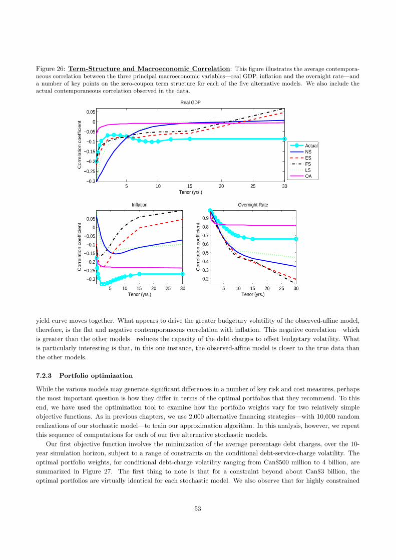
Figure 26: Term-Structure and Macroeconomic Correlation: This figure illustrates the average contempora-neous correlation between the three principal macroeconomic variables—real GDP, inflation and the overnight rate—anda number of key points on the zero-coupon term structure for each of the five alternative models. We also include theactual contemporaneous correlation observed in the data.

5 10 15 20 25 30−0.3

−0.25

−0.2

−0.15

−0.1

−0.05

0

0.05

Tenor (yrs.)

Co

rre

latio

n c

oe

ffic

ien

t

Real GDP

5 10 15 20 25 30

−0.3

−0.25

−0.2

−0.15

−0.1

−0.05

0

0.05

Co

rre

latio

n c

oe

ffic

ien

t

Tenor (yrs.)

Inflation

5 10 15 20 25 30

0.2

0.3

0.4

0.5

0.6

0.7

0.8

0.9

Co

rre

latio

n c

oe

ffic

ien

t

Tenor (yrs.)

Overnight Rate

ActualNSESFSLSOA

yield curve moves together. What appears to drive the greater budgetary volatility of the observed-affine model,therefore, is the flat and negative contemporaneous correlation with inflation. This negative correlation—whichis greater than the other models—reduces the capacity of the debt charges to offset budgetary volatility. Whatis particularly interesting is that, in this one instance, the observed-affine model is closer to the true data thanthe other models.

7.2.3 Portfolio optimization

While the various models may generate significant differences in a number of key risk and cost measures, perhapsthe most important question is how they differ in terms of the optimal portfolios that they recommend. To thisend, we have used the optimization tool to examine how the portfolio weights vary for two relatively simpleobjective functions. As in previous chapters, we use 2,000 alternative financing strategies—with 10,000 randomrealizations of our stochastic model—to train our approximation algorithm. In this analysis, however, we repeatthis sequence of computations for each of our five alternative stochastic models.

Our first objective function involves the minimization of the average percentage debt charges, over the 10-year simulation horizon, subject to a range of constraints on the conditional debt-service-charge volatility. Theoptimal portfolio weights, for conditional debt-charge volatility ranging from Can$500 million to 4 billion, aresummarized in Figure 27. The first thing to note is that for a constraint beyond about Can$3 billion, theoptimal portfolios are virtually identical for each stochastic model. We also observe that for highly constrained

53

Figure 27: Some Optimal Portfolio Weights: This figure illustrates the optimal portfolio weights—for each of thefive stochastic models—when the optimizer seeks to minimize total discounted debt charges over the 10-year simulationhorizon subject to a range of constraints on conditional debt-charge volatility.

0.5 1 1.5 2 2.5 3 3.5 40

50

100Nelson−Siegel

Constraint (Can$ billions)

Por

tfolio

wei

ght (

%)

1 2 3 40

50

100Exponential Spline

Constraint (Can$ billions)

Por

tfolio

wei

ght (

%)

1 2 3 40

50

100Fourier Series

Constraint (Can$ billions)

Por

tfolio

wei

ght (

%)

1 2 3 40

50

100OLS

Constraint (Can$ billions)

Por

tfolio

wei

ght (

%)

1 2 3 40

50

100Observed Affine

Constraint (Can$ billions)

Por

tfolio

wei

ght (

%)

RRB30y10y5y2y1y6m3m

optimizations (i.e., around Can$500–600 million), the exponential-spline and Fourier series models, unlike theother approaches, recommend a small, although non-zero, allocation to 30-year nominal bonds. We suspectthat this is due to the decreasing yield-curve volatility generated by these models and the relatively small costdifferences between 10- and 30-year debt in these models. As well, the observed-affine model reduces the relianceon 10-year debt more quickly than the Nelson-Siegel and OLS models, given its relatively higher assessment ofthe cost. Finally, RRBs are not present for any of the models.

The second optimization, described in Figure 28, seeks again to minimize the average percentage debt charges,albeit with a restriction on the refixing share of debt. Here we observe that only the Nelson-Siegel and OLSmodels recommend a significant allocation to 10-year nominal bonds for lower refixing share of debt constraints.We suspect that this is due to the relatively flat yield curves generated by these models, which suggests that thereare fewer cost savings to be gained by issuing short-term debt. For the same reason, we also observe that theexponential-spline, the Fourier-series and the observed-affine models all recommend 3- and 6-month treasury billallocations more quickly as we increase the refixing share of debt. The steeper short-term yield curves forecastby these models make this more cost effective.

7.3 Conclusion

The important conclusion from this analysis is that different models of the stochastic environment, estimatedwith the same data, can yield rather different results. The differences show up in the average shape of the yieldcurve, the volatility of the yield curve, and correlation structure among and between the yield curve and the

54

Figure 28: Some More Optimal Portfolio Weights: This figure illustrates the optimal portfolio weights—foreach of the five stochastic models—when the optimizer seeks to minimize total discounted debt charges over the 10-yearsimulation horizon subject to a range of constraints on the refixing share of debt.

25 30 35 40 45 50 55 60 65 70 750

50

100Nelson−Siegel

Constraint (%)

Por

tfolio

wei

ght (

%)

30 40 50 60 700

50

100Exponential Spline

Constraint (%)

Por

tfolio

wei

ght (

%)

30 40 50 60 700

50

100Fourier Series

Constraint (%)

Por

tfolio

wei

ght (

%)

30 40 50 60 700

50

100OLS

Constraint (%)

Por

tfolio

wei

ght (

%)

30 40 50 60 700

50

100Observed Affine

Constraint (%)

Por

tfolio

wei

ght (

%)

RRB30y10y5y2y1y6m3m

macroeconomic variables. These differences manifest themselves in the form of differing forecasts of key risk andcost characteristics for a given financing strategy. In this analysis, we found that in some cases these differenceswere small, whereas in others they were important. This finding applies to both the examination of a singlefinancing strategy and the optimization across the range of all admissible financing strategies. The bottom line,therefore, is that, in performing debt-strategy analysis, we cannot afford to ignore model risk.

55

8 The Macroeconomy

This chapter examines the interaction of macroeconomic variables and the term structure of interest rates, aswell as the sensitivity of the model results to macroeconomic and financial shocks.

In the previous chapter, we examined how alternative models describing the macroeconomy and the termstructure of interest rates can lead to different results. In this chapter, we focus on a single model—the Nelson-Siegel model—and walk through a number of detailed model diagnostics to better understand the interactionbetween the key components of the macroeconomy and the interest rate environment. Such analysis is importantto verify that the interaction between key variables is both correct and consistent. As previously discussed, theinteraction between the macroeconomy and interest rates will have important implications for the determinationof the government’s funding requirement and the relative attractiveness of inflation-linked debt. These diagnosticsare also important to ensure that the sensitivity analysis can reasonably be performed in the context of this model.In particular, we want to examine how an initial shock to output, inflation or the shape of the yield curve mightimpact the portfolio allocations. Such analysis is useful only if the interactions between the key stochasticvariables are correctly specified. Our diagnostic efforts, therefore, are designed to understand these interactions.

This chapter is organized into four sections. In the first section, we focus on model diagnostics. The principaldiagnostic tool, given the reduced-form nature of our model, is the impulse-response function. This section ishighly detailed to provide comfort that due diligence has been performed on the model, but is not required foranalyzing the impact of macroeconomic changes on model results. In the second section, we turn to examine howan equally weighted portfolio reacts to shocks to key variables. The objective in that section is to understandhow the shocks to the key stochastic variables translate into different risk and cost characteristics for a givenfinancing strategy. The third section will provide optimization results for alternative long-term values in themodel. Finally, the fourth section will make some concluding remarks.

8.1 The stochastic model

In an effort to mitigate model risk, as was described in Chapter 7, the debt-strategy model employs five alter-native models to describe the future evolution of macroeconomic and interest rate variables. These models haverather different foundations and various implications for the dynamics of the stochastic environment. Fortu-nately, however, the interactions between macroeconomic and interest rate variables in each of the models arequite similar; this implies that examining the interactions within the context of the Nelson-Siegel model shouldgive us a reasonably good idea of the interactions for all of the models. In particular, the joint dynamics ofthe macroeconomy and interest rates are represented in a VAR, which means that the current values of thestochastic variables depend on their past values. Current output, for example, depends on past output as wellas past inflation, monetary policy and yield-curve variables. The advantage of VARs is that they provide arich description of the dependence between a collection of variables. In other words, such a model permits eachvariable to have an influence on every other variable in the system.

The macroeconomic variables included in our joint model of the macroeconomy and the term structure ofinterest rates include the output gap, the overnight rate and the annual rate of change in the core consumerprice index (CPI).67 These factors represent the level of real economic activity relative to potential, the monetarypolicy instrument and the rate of price inflation, respectively. We use this set of variables since it is consideredto be the minimum set of factors needed to capture basic macroeconomic dynamics. The growth in potentialoutput is included as an exogenous variable to the system.68 It is included to infer real GDP growth, which isinstrumental in the estimation of the debt model’s primary balance.69 We also include total CPI exogenously,

67The output-gap series used in our analysis is the estimate produced by the Bank of Canada and is converted from quarterly to

monthly frequency using a cubic spline.68An exogenous variable influences the other variables in the system, but is not directly influenced by the other variables.69More details on this are provided in Chapter 6.

56

since this quantity is required for the pricing of inflation-linked debt. The term-structure variables are the level,slope and curvature of the zero-coupon yield curve. An extensive literature shows that these three factors aresufficient to explain more than 95 per cent of term-structure variability. Armed with this set of variables, ourstochastic model is able to generate key macroeconomic shocks to inflation, interest rates, aggregate demand,technology and supply.

One disadvantage of the VAR approach is that the relatively large number of reduced-form model parameterscreate a general difficulty with parameter interpretation. Interpreting the sign and statistical significance of theparameters for a VAR of even moderate dimension is a very difficult, and often impossible, task. Moreover, R2

measures are not terribly helpful. For this reason, other tools are used to gauge the usefulness of a VAR model.The first tool involves the examination of the out-of-sample forecasting ability of a given VAR specification.Since the ability of these models to forecast future interest rate outcomes has been extensively addressed inBolder and Liu (2007), we will not cover this diagnostic approach. Another tool for the examination of VARs isthe impulse-response function. An impulse-response function traces the effect of a one standard-deviation shockto one of the error terms of the VAR on current and future values of the endogenous variables.70 In other words,imagine that there was a one standard-deviation surprise in the current value of inflation: the impulse-responsefunction would measure the corresponding impact, in the absence of any additional noise, on the other variablesin the VAR.

In short, impulse-response functions are invaluable in understanding the structure of a VAR model, becausethey succinctly describe the model’s dependence structure. In what follows, we will examine the key impulse-response functions for our standard VAR model. Before turning to the VAR impulse-response functions, however,it will be useful to outline the dynamics of a traditional small-scale structural macroeconomic model. This willprovide a reference point for the analysis of the VAR dynamics.

Typical small macroeconomic models used for monetary policy analysis—often termed New-Keynesian models—generally include three key variables: the output gap, inflation and the monetary policy rate. In these models,current output depends positively on past/expected output and negatively on the real interest rate. Currentinflation is determined by an expectations-augmented Phillips curve, whereas inflation is positively influenced bypast/expected inflation and by the size of the current output gap. The monetary policy rate is determined usingan estimated or calibrated Taylor rule, in which the short-term interest is set according to current/expectedinflation and the output gap. In such a model, an aggregate demand shock would increase the output gap,and in turn raise inflation. This would cause the monetary authorities to increase the policy rate, which wouldeventually close the output gap and bring inflation back in line with their target.

We can now examine the impulse-response functions to better understand our VAR dynamics. Figure 29describes the impact (response) on the macroeconomic variables to a one standard-deviation shock (impulse)to the macroeconomic variables. The first row, for example, illustrates the impact on the output gap, the coreinflation rate, and the ON-rate for a shock to the output gap. We observe that the overnight rate displays apositive response to a rise in the output gap, which is consistent with a typical monetary policy reaction function.In contrast, when examining the second row of Figure 29, we observe that the overnight rate falls with a positiveshock to inflation. This is a seemingly counterintuitive finding.

However, the impulse-response functions indicate that a positive shock to inflation has the typical responseof reducing output.71 Hence, the negative response of the overnight rate to a positive inflation shock can beexplained by the fact that output displays a greater degree of persistence over the estimation sample thaninflation. That is, core inflation comes back to target more quickly than output. Indeed, the output gap displays

70The Cholesky decomposition is used to identify underlying structural shocks from the reduced-form shocks. Changing the

ordering of the variables used for identification of the structural shocks in this approach will, generally, lead to different results. In

this analysis, however, changing the ordering produced only minor differences in the impulse-response functions. The order presented

in this analyis is level, curvature, slope, output gap, core inflation and the overnight rate.71The negative response of the output gap to a positive shock to both inflation and the overnight rate is consistent with an

aggregate demand shock in small macro models.

57

Figure 29: Macro-Macro Impulse-Response Functions: This figure illustrates the impulse-response functionsof the macroeconomic variables for shocks to the macroeconomic variables. The first row demonstrates the response onthe output gap, core inflation and the overnight rate to a shock to the output gap. The second row illustrates the response,for the same set of variables, to an inflation shock. The final row outlines the results for a shock to the overnight rate.

1 2 3 4 5−0.2

−0.1

0

0.1

0.2

Output Gap Response

Out

put−

Gap

impu

lse

1 2 3 4 51.8

1.9

2

2.1

2.2Core π Response

1 2 3 4 5

3.8

4

4.2

4.4

ON−Rate Response

1 2 3 4 5−0.2

−0.1

0

0.1

0.2

Cor

e π

impu

lse

1 2 3 4 51.8

1.9

2

2.1

2.2

1 2 3 4 5

3.8

4

4.2

4.4

1 2 3 4 5−0.2

−0.1

0

0.1

0.2

Time (yrs.)

ON

−R

ate

impu

lse

1 2 3 4 51.8

1.9

2

2.1

2.2

Time (yrs.)1 2 3 4 5

3.8

4

4.2

4.4

Time (yrs.)

a high degree of persistence, taking about two years to return to its initial value following an aggregate demandshock.72 Inflation, conversely, exhibits little persistence, falling back to its initial value following a price shockwithin 10 months. This observation suggests that the monetary authorities will react more to the fall in outputthan to the rise in inflation, because a stronger reaction is required to increase output than is required to decreaseinflation.

A positive shock to the output gap raises inflation—which is consistent with the results of small monetarypolicy macroeconomic models—while shocks to the overnight rate and to the yield-curve factors have littleimpact. In fact, statistical tests indicate that inflation can be treated as an exogenous variable to the VARsystem.73 This is consistent with studies that have found that the inflation process, since the introduction ofinflation targeting in the early 1990s, is well forecast by a simple constant.74 This result stems from the factthat the Bank of Canada has been generally successful in keeping inflation expectations well anchored and that,on average, shocks to inflation do not permanently impact expectations.

Figure 30 illustrates the response of the financial variables to a one standard-deviation shock to the macroe-conomic variables. The first row outlines the impact on the level, slope and curvature of a shock to the outputgap. As before, the second row of Figure 30 illustrates the response, for the same set of variables, to an infla-

72Incidentally, although it is not shown here, an exogenous shock to potential output growth leads to a decline in the output gap,

consistent with a lagged adjustment of demand to supply shocks.73We principally employ the so-called Wald exogeneity test. Loosely speaking, this test permits a multivariate examination of the

statistical significance between the covariance terms in the endogenous variables of a linear system.74See Demers (2003) for a more detailed discussion of this issue.

58

Figure 30: Macro-Finance Impulse-Response Functions: This figure illustrates the impulse-response functionsof the financial variables for shocks to the macroeconomic variables. The first row demonstrates the response of the level,slope and curvature of the zero-coupon curve to a shock to the output gap. The second row illustrates the response, forthe same set of variables, to an inflation shock. The final row outlines the results for a shock to the overnight rate.

1 2 3 4 5

6

6.2

6.4

Level Response

Out

put−

Gap

impu

lse

1 2 3 4 5

2.2

2.4

2.6

Slope Response

1 2 3 4 5

0.4

0.6

0.8

Curvature Response

1 2 3 4 5

6

6.2

6.4

Cor

e π

impu

lse

1 2 3 4 5

2.2

2.4

2.6

1 2 3 4 5

0.4

0.6

0.8

1 2 3 4 5

6

6.2

6.4

Time (yrs.)

ON

−R

ate

impu

lse

1 2 3 4 5

2.2

2.4

2.6

Time (yrs.)1 2 3 4 5

0.4

0.6

0.8

Time (yrs.)

tion shock while the final row outlines the results for a shock to the overnight rate. The level factor is highlycorrelated with the nominal 10-year government bond yields as well as with measures of inflation. This suggestsa relationship between the level of the yield curve and inflationary expectations. We observe in the first columnof Figure 30, however, that shocks to core inflation, the output gap and the overnight rate appear to producerelatively modest responses in the level factor. Again, statistical tests indicate that the level factor could alsobe treated as an exogenous variable in the VAR system. This result is consistent with inflationary expectationsbeing well anchored in Canada over the estimation period.

The slope factor exhibits a negative response to an increase in the overnight rate. What appears to behappening is that an increase in the output gap leads to an increase in the overnight rate (see Figure 29), whichin turn leads to an increase in short-term interest rates and a subsequent decrease in the slope of the yield curve.Indeed, the overnight rate and the yield-curve slope are strongly negatively correlated. The reason is that withanchored inflationary expectations, we should expect to see increases (decreases) in the overnight rate associatedwith decreases (increases) in the slope of the yield curve. This is because the overnight rate and short-terminterest rates are closely linked. Shocks to core inflation, therefore, generate decreases in the overnight rate,which trigger an increase in the slope of the yield curve.

Initially, the positive reaction of the slope to a positive shock to the overnight rate is a bit puzzling. Figure 29,however, demonstrates that a shock to the overnight rate persists only for a very short period and eventuallyleads to a decrease in the overnight rate—the consequence, therefore, is an increase in the yield-curve slope. Wealso observe that both the slope and curvature factors display a high degree of persistence, requiring more than

59

Figure 31: Finance-Macro Impulse-Response Functions: This figure illustrates the impulse-response functionsof the macroeconomic variables for shocks to the financial variables. The first row demonstrates the response of the outputgap, core inflation and the overnight rate to a shock to the level. The second row illustrates the response, for the sameset of variables, to a slope shock. The final row outlines the results for a shock to curvature.

1 2 3 4 5−0.2

−0.1

0

0.1

0.2

Output−Gap Response

Leve

l im

puls

e

1 2 3 4 51.8

1.9

2

2.1

2.2Core π Response

1 2 3 4 5

3.8

4

4.2

4.4

ON−Rate Response

1 2 3 4 5−0.2

−0.1

0

0.1

0.2

Slo

pe im

puls

e

1 2 3 4 51.8

1.9

2

2.1

2.2

1 2 3 4 5

3.8

4

4.2

4.4

1 2 3 4 5−0.2

−0.1

0

0.1

0.2

Time (yrs.)

Cur

vatu

re im

puls

e

1 2 3 4 51.8

1.9

2

2.1

2.2

Time (yrs.)1 2 3 4 5

3.8

4

4.2

4.4

Time (yrs.)

two years each to return to their initial values following an aggregate demand shock.The yield-curve curvature factor is highly correlated with economic activity. Indeed, the contemporaneous

correlation between real GDP and the curvature factor is slightly greater than 0.40. A shock to the output gap,therefore, leads to an increased curvature, while increases in core inflation, which dampen growth, negativelyimpact the curvature of the yield curve.

Figure 31 demonstrates the response of the macroeconomic variables to a one standard-deviation shock tothe financial variables. Each row outlines the impact on the output gap, core inflation and the overnight rateof a one standard-deviation shock to the yield-curve level, slope and curvature, respectively. The level factorappears to have little impact on any of the macroeconomic variables. As we can see in Figure 32, a shock tothe level factor is persistent and reasonably large, but it does not have a large impact on the macroeconomy. Apositive shock to the slope variable, however, generates, as expected, a decrease in the overnight rate, which inturn leads to an increase in the output gap. Moreover, a positive shock to curvature raises the output gap. Thisis consistent with typical forward-looking macroeconomic models, where expectations of greater future economicactivity and inflation lead to higher contemporaneous output and inflation.

Level, slope and curvature factors obtained from traditional statistical analysis are, by construction, indepen-dent. When these factors are extracted from the Nelson-Siegel model, however, we observe a strong contempo-raneous correlation between the level and slope factors. In addition, the level and curvature factors demonstratea modest positive contemporaneous correlation. Figure 32 shows the impulse-response functions of the financialvariables for shocks to the financial variables. Again, each row demonstrates the response of the level, slope and

60

Figure 32: Finance-Finance Impulse-Response Functions: This figure illustrates the impulse-response func-tions of the financial variables for shocks to the financial variables. The first row demonstrates the response of the level,slope and curvature of the yield curve to a shock to the level. The second row illustrates the response, for the same setof variables, to a slope shock. The final row outlines the results for a shock to curvature.

1 2 3 4 5

6

6.2

6.4

Level Response

Leve

l im

puls

e

1 2 3 4 5

2.2

2.4

2.6

Slope Response

1 2 3 4 5

0.4

0.6

0.8

Curvature Response

1 2 3 4 5

6

6.2

6.4

Slo

pe im

puls

e

1 2 3 4 5

2.2

2.4

2.6

1 2 3 4 5

0.4

0.6

0.8

1 2 3 4 5

6

6.2

6.4

Time (yrs.)

Cur

vatu

re im

puls

e

1 2 3 4 5

2.2

2.4

2.6

Time (yrs.)1 2 3 4 5

0.4

0.6

0.8

Time (yrs.)

curvature of the yield curve to a shock to the level, slope and curvature factors, respectively.An increase in the level of the yield curve appears to generate a persistent increase in the slope of the

yield curve, although it has little impact on the yield-curve curvature. These results seem to be driven by thepreviously mentioned correlation structure. Interestingly, a shock to the slope factor generates a lagged decreasein the level of the yield curve as well as a slight increase in the curvature. The slope returns back to its long-termmean within about 18 months and then actually falls below this value. Presumably, this is what is driving thefall in the level. Finally, a curvature shock generates a modest, but persistent, increase in the level of the yieldcurve and a slight decrease in the yield-curve slope.

The basic impulse-response functions, then, are generally consistent with the results of traditional small-scalestructural macroeconomic models. The one exception is the response of the overnight rate to an inflationaryshock, although this can be explained by the lack of persistence of inflation and the forward-looking nature ofCanadian monetary policy. Nevertheless, we also estimated a structural VAR—in which a standard Taylor typerule was calibrated to explain the dynamics of the overnight rate—to address this issue. This model producedpersistence in the inflation process, however, that was fundamentally inconsistent with the historical evidence.As a consequence of this distortion, we elected not to use the structural specification.

As a final point, we find that the macroeconomic variables have a significant influence on the term structure.Moreover, the term-structure factors also appear to have an important influence on the macroeconomic variables.While this is not entirely consistent with the findings in the literature, it does seem reasonable given the forward-looking nature of monetary policy in Canada and the expectational information contained in the term-structure

61

factors.75

8.2 Impact of shocks on model results

We next focus on how shocks to our six principal stochastic variables impact the model results. This is, in fact, anatural extension of the analysis in the previous section. We are essentially asking “what happens to the risk andcost characteristics associated with a given financing strategy when the starting point of one of the stochasticvariables is shocked?” At most points in this paper we begin the simulation of the stochastic system using thefinal datapoints in our historical time series.76 In this analysis, however, we start from the long-term mean toprovide a clean view of the interaction of the variables without mean reversion effects clouding the results. Usingthe long-term mean starting point, therefore, we again apply the idea of an impulse-response function with a onestandard-deviation shock to each of the stochastic variables. We then run the simulation algorithm using thesealternative starting points.

Let us consider an example. A shock to the output gap, using the results from the previous section, should, onaverage, lead to a slight increase in core inflation, the overnight rate and the yield-curve level, with a simultaneousdecrease in the slope of the yield curve.77 What impact, however, does this output-gap shock have on the riskand cost characteristics of a given financing strategy? Figure 33 addresses this question in part by demonstratingthe impact on the zero-coupon curve of a one standard-deviation shock to the simulation’s starting point foreach of the key stochastic variables.

The top-left quadrant of Figure 33 describes the average distance between the unshocked curves across 10,000simulations. The thick dashed blue line from the origin represents the results for an unshocked simulation.Observe that a shock to the level and curvature factors leads to the highest zero-coupon curves. While the levelshock is self-explanatory, the positive and persistent increase of the level factor in response to a curvature shockappears to explain the increase in the expected zero-coupon curve. An output-gap shock also leads to a generalincrease in interest rates. This is consistent with the impulse-response analysis, insofar as the associated increasein the overnight rate and the yield-curve level should generate slightly higher zero-coupon curves.

A positive shock to the yield-curve slope appears to arise more through an decrease in short-term interestrates than through an increase in long-term rates. Indeed, longer-term rates appear to fall in reaction to apositive shock to the yield-curve slope. The consequence, therefore, is generally lower interest rates in responseto a shock to the slope. A positive inflation shock appears to slightly decrease interest rates; this is consistentwith the previous analysis, which indicated a negative output-gap and overnight-rate response to an inflationaryshock. Finally, the overnight shock leads to a decrease in interest rates, although it does not appear to deviatesubstantially from the base scenario. This can be explained by Figure 29, where an initial shock to the overnightrate generates a decrease in output and a subsequent decrease in the overnight rate. The total result, therefore,is lower interest rates.

We also observe from Figure 33 that the standard deviation of the zero-coupon curve (see the top-rightquadrant) does not substantially differ for the various shocks to our stochastic variables. None of the shocksleads to a change of more than five basis points from the base, unshocked scenario—considering that the overallzero-coupon volatility ranges from 80 to 120 basis points, this is not substantial. It is also not surprising, sinceonly the starting points differ between the simulations. That is, the dynamics of the state variables do notchange in response to a shock to the starting values. As such, there should be no change in the variability ofzero-coupon outcomes. Moreover, the bottom two quadrants of Figure 33 indicate that the 3-month and 10-year

75The academic evidence is somewhat mixed. Some studies indicate a rather weak influence of macroeconomic variables in the

term structure, while other studies demonstrate a stronger relationship.76The data used in this analysis begin in November 1993 and terminate in February 2007. The starting point for the simulation

of the stochastic system, therefore, would typically be February 2007.77We say “on average” because the simulation, unlike the impulse-response analysis in the previous section, also includes the usual

amount of noise.

62

Figure 33: Impact of One Standard-Deviation Shocks on Term-Structure Outcomes: This figure illus-trates the impact of a one standard-deviation shock to the starting point of the simulation for each of the key stochasticvariables: level, slope, curvature, the output gap, core inflation and the overnight rate. For each shock, the results arepresented as the distance of the average zero-coupon curve, the zero-coupon curve volatility, the average evolution of the3-month rate and the average evolution of the 10-year rate from the base, unshocked scenario. The thick dashed blue linefrom the origin, therefore, represents an unshocked simulation.

5 10 15 20 25 30−8

−6

−4

−2

0

2

4

6

Tenor (yrs.)

Ba

sis

po

ints

Distance from Base Zero−Coupon Curve (bps.)

5 10 15 20 25 30−3

−2

−1

0

1

2

3

Tenor (yrs.)

Ba

sis

po

ints

Distance from Base Zero−Coupon Curve Volatility

2 4 6 8 10

−30

−20

−10

0

10

Time (yrs.)

Ba

sis

po

ints

Distance from Average Short−term (3M) Rates

2 4 6 8 10

−10

−5

0

5

10

15

Time (yrs.)

Ba

sis

po

ints

Distance from Average Long−term (10Y) Rates

Base

Level

Slope

Curve

Y−Gap

Core πO/N

zero-coupon rates essentially converge from their alternative starting points to their long-term mean within threeto four years.

Figure 34 shows how the zero-coupon curve results in Figure 33 translate into model results. In particular,Figure 34 illustrates the impact of each shock on the expected debt charges, debt-charge volatility and relativecost-at-risk (CaR) for an equally weighted portfolio of 3-, 6- and 12-month treasury bills; 2-, 5-, 10- and 30-yearnominal bonds; and 30-year inflation-linked bonds. Again, the results are presented as the distance from thebase, unshocked scenario. Those shocks that generate higher interest rates translate, unsurprisingly, into higherdebt charges. Thus, shocks to the level of the yield curve, the curvature of the yield curve and the output gapgenerate higher expected debt-service charges. Conversely, shocks to the slope of the yield curve, core inflationand the overnight rate generate lower expected debt-service charges. In all cases, the magnitude of the differencesfrom the unshocked scenario dissipate as we move through time and further away from the starting-value shock.

The small differences in zero-coupon curve volatility evident in Figure 33 are consistent with the minimaldifferences in debt-charge volatility and relative CaR for the different shocks. The differences in Figure 33 appearprimarily because of simulation noise. Again, the shocks influence the starting point of the simulations, not thedynamics of the stochastic system. The consequence is that the level of debt-service charges is impacted, whereastheir dispersion remains the same. In other words, shocks to the starting point of the stochastic system have costimplications, but not risk implications, for a given financing strategy. One could, of course, construct a more

63

Figure 34: Impact of One Standard-Deviation Shocks on Equally Weighted Portfolio: This figure il-lustrates the impact of a one standard-deviation (i.e., 2.3 standard-deviation) shock to the starting point of the simulationfor each of the key stochastic variables on the expected debt charges, debt-charge volatility and relative cost-at-risk (CaR)of an equally weighted portfolio.

1 2 3 4 5 6 7 8 9 10−1.5

−1

−0.5

0

0.5

1

Time (yrs.)

Ca

n$

bill

ion

s

Distance from Base Expected Debt−Charges

BaseLevelSlopeCurveY−GapCore πO/N

2 4 6 8 10−0.06

−0.04

−0.02

0

0.02

0.04

0.06

Time (yrs.)

Ca

n$

bill

ion

s

Distance from Base Debt−Charge Volatility

2 4 6 8 10−0.2

−0.15

−0.1

−0.05

0

0.05

0.1

0.15

Time (yrs.)

Ca

n$

bill

ion

sDistance from Base Relative CaR

complex model, whereby the volatility of the stochastic system varies with the level of the individual stochasticvariables.78 This, however, cannot be accommodated in the current model.

8.3 Testing alternate long-term values

The above analysis demonstrated that shocks to the financial and macroeconomic variables did not cause changesto key risk measures. Furthermore, even if the risk measures were affected, it would have to be in an asymmetric(with respect to financing instruments) manner to be of great concern. Therefore, from the perspective ofselecting an optimal portfolio, the impact of the shocks is not “portfolio-moving.” In this section we analyzewhat happens to optimal portfolios when key components of the system are changed. These will be the slope ofthe yield curve and the yield-volatility structure.79

First, we will examine the results, using conditional debt-charge volatility as the risk constraint, when chang-ing the yield-curve slope. When generating scenarios for the model, one can specify long-term values for financialor macroeconomic variables, or allow the model to determine the long-term values. The curves are the averageyield curves for each of the three long-term value specifications, with the long-term means as the starting point.In this case, the financial variables’ long-term values were changed to give the red and green lines in Figure 35.

78If increasing interest rates were, for example, more variable, then a shock to output might actually increase the risk of a given

financing strategy.79Analysis in this section uses a more recent dataset, and therefore base results will not match with results from Chapter 5.

64

Figure 35: Different Yield-Curve Slopes: The graph on the left shows the three different yield curves (Flatter,Base, Steeper) that were tested with the model. The expected cost-risk trade-off from the optimizations using conditionaldebt-charge volatility are shown in the graph on the right.

1 2 3 42.5

3

3.5

4

4.5

5

5.5

6Expected Cost Frontiers

Conditional Debt−Charge Volatility (Can$ billions)

Expe

cted c

ost (%

)

FlatterBaseSteeper

0 10 20 302

2.5

3

3.5

4

4.5

5

5.5

6

6.5

Tenor (yrs.)

Intere

st rat

e (%)

Altering the Slope of the Yield Curve

FlatterBaseSteeper

The blue line uses the model-determined long-term values. Long-term yields have remained relatively close inthe three curves, while short-term rates are very different.

One would expect the different curves to impact the expected cost frontiers and the portfolio weights. Thesecond pane of Figure 35 shows the expected cost frontiers, and it is immediately obvious how much the yield-curve slope impacts these frontiers. The slope of the expected cost frontiers is directly related to the slopeof the yield curve, and one can see that the range of the frontiers is also affected. The frontiers level off attheir respective minimum cost portfolios, with these differing between the curves because the cost savings fromhaving more short-term debt in the portfolio (at a higher volatility) are different across the curves. Specifically,the lower cost savings in the flatter curve lead to less short-term debt in the minimum cost portfolio, and alower conditional debt-charge volatility of that portfolio. This can be seen in Figure 36. Conversely, and notsurprisingly, long-term debt plays a larger role the flatter the yield curve, with this extending to the 5-year sectoras well.

Table 5: Financing Strategies: This table outlines the optimal financing strategies for the flatter, base and steeperyield-curve scenarios at a conditional debt-charge volatility of Can$2 billion.

Financing StrategiesDebt Type TenorFlatter Base Steeper

3-month 7% 11% 13%6-month 0% 0% 0%1-year 10% 11% 9%2-year 21% 26% 25%3-year 14% 15% 19%5-year 42% 36% 34%

10- year 0% 0% 0%

Nominal

30-year 0% 0% 0%Real 30-year 6% 0% 0%

Another relevant avenue for analysis is comparing the optimal portfolios at a given risk level. Table 5 showsthe optimal portfolio for a conditional debt-charge volatility level of two, for all three yield curves. Although notidentical, they have a significant amount in common. Specifically, they each have a large allocation to 5-year

65

Figure 36: Portfolio Weights for Different Yield Curves: This figure illustrates the portfolio weights for threedifferent yield curves. The range of outcomes is lower the flatter the yield curve. As well, the flatter the yield curve, thelower the amount of short-term debt in the minimum cost portfolio, and in general.

0.5 1 1.5 2 2.5 3 3.5 40

20

40

60

80

100Model−Determined Curve

Conditional Debt−Charge Volatility (Can$ billions)

Po

rtfo

lio w

eig

ht (

%)

1 2 3 40

20

40

60

80

100Flatter Curve

Conditional Debt−Charge Volatility (Can$ billions)

Po

rtfo

lio w

eig

ht (

%)

1 2 3 40

20

40

60

80

100Steeper Curve

Conditional Debt−Charge Volatility (Can$ billions)

Po

rtfo

lio w

eig

ht (

%)

RRB30y10y5y3y2y1y6m3m

bonds; smaller, but significant allocations to 2- and 3-year bonds; about a 20 per cent allocation to treasurybills; with a small to non-existent allocation in RRBs as the only long-term debt. This is significant because if aparticular optimal portfolio is targeted from a given scenario, changes in the average yield curve will not greatlyimpact its efficiency or risk level. This result is to be expected, since yield volatilities remained the same acrossthe different average yield-curve scenarios.

A natural next step in the analysis is to look at the effects of changing the volatility structure of yields.Figure 37 has the relevant graphs for the change in volatility structure. The volatility structure was flattenedand increased.80 The effect of this on the expected cost-risk trade-off was higher cost at a given risk level. Thisis not surprising, since to reach a given conditional debt-charge volatility level, one must have more longer-termdebt. One can see graphically that the lowest cost portfolios are not significantly different, nor do they havesignificantly different expected costs. This was anticipated because the average yield curve did not change. Theydo, however, have different conditional debt-charge volatilities. Furthermore, the bottom panes of Figure 37 showthat, unlike when changing the slope of the yield curve, changing the yield volatilities will change the optimalportfolio at a given risk level.

80Although the change will affect the cost volatility for a given financing instrument, the effect will not be one-to-one. Costvolatility is significantly affected by the frequency of rollover, as well as yield volatility.

66

Figure 37: Altering Yield Volatilities: The top-left graph shows the model-determined and flatter yield volatilities.The top-right graph shows the expected cost differences between the two yield-volatility scenarios. The two bottom graphsshow the financing strategies associated with the expected cost curves in the top-right graph.

3m 6m 1y 2y 3y 5y 10y 30yRRB0

20

40

60

80

100

120

140Yield Volatilities

Instrument

Vol

atili

ty (

bps)

Model−DeterminedFlat

1 2 3 40

20

40

60

80

100Model−Determined Yield Volatilities

Conditional Debt−Charge Volatility (Can$ billions)

Por

tfolio

wei

ght (

%)

1 2 3 4 54.2

4.4

4.6

4.8

5

5.2

5.4

5.6

Cost−Risk Trade−off

Conditional Debt−Charge Volatility (Can$ billions)

Exp

ecte

d C

ost (

per

cent

)

1 2 3 4 50

20

40

60

80

100Flat Yield Volatilities

Conditional Debt−Charge Volatility (Can$ billions)

Por

tfolio

wei

ght (

%)

Model−DeterminedFlat

RRB30y10y5y3y2y1y6m3m

8.4 Conclusion

This chapter examined the nature of the interaction between the individual macroeconomic and financial variablesin our stochastic system. Such diagnostic analysis is critical for understanding, and ensuring the consistency of,our stochastic system. Our principal conclusion is that the impulse-response functions from our reduced-formVAR model, which describes the dependence structure of our stochastic system, are generally consistent withthe results of traditional small-scale structural macroeconomic models. Moreover, shocks to the starting valuesof the macroeconomic and financial variables potentially impact the cost of a given financing strategy, but notits risk.

In addition, we examined how optimal portfolios and expected cost frontiers changed when key aspects ofthe system are changed. We found that, although significantly different yield curves will give different ranges ofcost-volatility outcomes, the portfolio at a given risk level is similar across the three average curves tested. Aswell, we found that altering yield volatility will impact the optimal portfolios at a given risk level.

67

9 The Issuance-Penalty Function

This final chapter considers the interaction between the amount of debt issuance and its associated cost. Inprinciple, a government’s financing decisions have an impact on the state of the macroeconomy and interestrates. A government’s decision, for example, to finance itself entirely with very short-term debt would havean impact on the financing costs of non-government entities. In particular, a surfeit of short-term, risk-freedebt could crowd out other borrowers; the consequence might be higher borrowing costs for these entities andcorrespondingly lower economic activity. In addition to this crowding-out effect at the short end, one mightexpect to observe difficulty in pricing and hedging longer-term issuance given the dearth of government supply—again, this could influence the level of interest rates and negatively impact economic activity. While this logic isquite reasonable, the stochastic model does not currently describe the interaction between the financing strategyand the macroeconomy. Why not? We do not endogeneously add the financing strategy into the macroeconomy,quite simply because we do not have the data to estimate anything meaningful.

For the effect of the issuance amount on yield, we have two choices. We can (i) ignore this effect or, (ii) usea relatively arbitrary approach to capture it. With the enhanced debt-strategy model, we opted for the secondapproach, which involves including an issuance-penalty function to capture this effect. Implicitly, therefore,we have decided that it is preferrable to attempt to describe this effect—and to have a rough approximationincluded in the model—than to ignore it. This chapter describes the logic behind this issuance-penalty functionand examines its influence on model results.81 The chapter is organized into two parts. The first part describesthe basic logic and structure of the penalty function and the second part examines how optimal portfolio weightsvary for different specifications of the penalty function.

9.1 The penalty function

The logic behind the issuance-penalty function is quite simple. If the government issues an excessively small orlarge amount of a given debt instrument in a given sector, it will possibly be at a higher yield than if it issueda more “reasonable” amount. Reasonable in this context implies that supply approximately equals demand andthat the issuance profile contributes to a liquid, benchmark issue. Imagine, for example, that the Canadiangovernment decided to issue only Can$100 million of 30-year nominal bonds in a given quarter, compared to atypical issue amount of more than Can$1 billion. One might expect that the government would have to pay aliquidity premium to issue such a small amount. It is more likely, however, that this would create substantialexcess demand from pensions and insurance companies, who use these long-tenor bonds to match their long-term liabilities. The consequence of such a small issuance amount, therefore, may actually be slightly betterissuance costs for the government—the difference between an increase or a decrease in cost as we decrease supplywill depend upon the demand schedule of investors and available substitutes. Conversely, imagine that thegovernment decided to issue Can$40 billion of 2-year bonds in a given quarter.82 Again, one can easily imaginethat it would be difficult for the market to absorb such a large amount of supply. We assume that such extremeissuance can be achieved, but that it has a cost, and that the government pays this cost in the form of highercoupons. The penalty function determines the magnitude of this increase to the coupon.

We can probably all agree, in principle, that small issuance amounts lead to either the payment of a liquiditypremium or a possible decrease in funding costs, and that large issuance amounts lead to the payment of aplacement or absorption premium. What is more difficult to agree on, however, is the magnitude of these effectsand when they begin and end. Unfortunately, these effects are generally impossible to estimate with statisticaltechniques. The reason is simple: we have no data. It is hard to know how much it would cost to issue Can$100millon of 30-year nominal bonds or Can$40 billion of 2-year bonds in a given quarter, since the government has

81The penalty functions provided in this chapter are not those currently used in the model.82It is not simply a case of absorbing a one quarter issuance amount. Given that the model uses fixed financing strategies, and

assuming a constant debt stock, this amounts to an every-quarter issuance amount.

68

never engaged in anything close to such issuance behaviour in the past.As a consequence, we find ourselves in uncharted territory. The inability to estimate the issuance-penalty

function implies that we must determine its mathematical form in a subjective fashion. While we have attemptedto do this in a reasonable and defensible manner, it should be stressed that there is an unavoidably arbitraryelement to this effort. As such, users and consumers of the debt-strategy model should be clearly aware of thelogic behind the construction of the issuance-penalty function.

The graphs in the following figures are for demonstration only. They generally show the form of the issuance-penalty functions, but do not represent those currently in use. One can see a flat portion at zero for both thecurves. This represents the non-penalized zone; issuance in this area can be done at prevailing market yields.Issuance above the upper bound of this zone, or below the lower bound of this zone, will have a change in yield(and coupon) based on the instrument and issuance level. The formulations below, and those not shown, areused in subsequent sections to evaluate the impact of the issuance-penalty functions on the model results. Inpractice, the issuance-penalty functions are updated regularly, so that they are reflective (to the best of ourability) of the current environment.

Figure 38: Sample Penalty: This figure illustrates a possible penalty, in basis points, associated with the 3-monthtreasury bill and 2-year bond. The lower bound on issuance for each is, of course, zero. The upper bound, conversely,represents the maximum amount of quarterly issuance possible, assuming that a Can$400 billion portfolio was fundedwith only that specific tenor.

0 50 100 150 200 250 300 350 400−20

−10

0

10

20

30

40

50

Bas

is p

oint

s

Quarterly Issuance (Can$ billions)

3−Month

0 5 10 15 20 25 30 35 40 45 500

20

40

60

80

100

120

Bas

is p

oint

s

Quarterly Issuance (Can$ billions)

2−year

The second part of the issuance-penalty function relates to its mathematical form. As we have alreadyestablished, we add a penalty to the par interest rate of each financing instrument when it falls below the lowerbound or above the upper bound. Logically, the size of the penalty should increase the further we deviate fromthe unpenalized boundary (i.e., the region where issuance does not impact market prices). A small reduction orincrease in issuance beyond the non-penalized range should not generate dramatic increases in cost. We opted,

69

therefore, for a functional form that increases non-linearly as the distance from the boundary increases. As such,the penalty is quite small for small movements outside the boundary, but increases exponentially for substantialdeviations. Essentially, the penalty function is a piecewise polynomial whereby issuance costs below the lowerbound, and above the upper bound, increase parabolically.83

The choices of the penalty-function parameters—that decide on the magnitude of the incremental cost tothe government for excessively large or small issuance—were initially made to provide reasonably conservativevalues. Figure 38 graphically demonstrates the magnitude of a sample issuance-penalty function for the 3-monthtreasury bill and the 2-year bond. The lower bound on issuance for each bill is, of course, zero. The upperbound, conversely, represents the maximum amount of quarterly issuance possible, assuming that a Can$400billion portfolio was funded with only that specific tenor. Note that the maximum penalty, for a situation wherethe entire portfolio is financed with only one tenor, leads to a 50 and 130 basis point penalty for the 3-month billand 2-year bond, respectively. When issuance falls below the lower issuance bound, however, the actual fundingrate is assumed to decrease for the 3-month treasury bill. The logic behind this choice is the strong institutionaldemand for risk-free short-term investments that can be classified as cash. We assume that there is a modestincrease in cost for the issuance of 2-year nominal bonds below the lower bound.

In the next section, we use the issuance-penalty functions in a portfolio-optimization exercise. It bearsrepeating that all the issuance-penalty functions presented in this chapter are for demonstration only. They areintended to show the general functional form and characteristics of the issuance-penalty functions, not to showtheir current iteration.

9.2 Optimal portfolio weights

The issuance-penalty functions should presumably have implications for the relative cost characteristics of dif-ferent financing strategies. Figure 38, for example, indicates that issuing entirely 3-month treasury bills willincrease the average issuance costs by approximately 50 basis points. This should lead to significantly largerdebt-service charges relative to a more balanced portfolio. This section attempts to understand the nature ofthese implications. If we attempt to minimize debt-service charges, subject to some form of risk constraint, wewould expect the optimizer to avoid a financing strategy composed entirely of 3-month treasury bills by virtueof its higher cost. Thus, we can see that the issuance-penalty function acts as something of a constraint againstextreme portfolio allocations.

To better understand how the issuance-penalty function impacts portfolio allocations, we perform a simpleexperiment. Specifically, we examine three alternative issuance-penalty specifications: the base penalty, a zero-issuance penalty and an extreme penalty function. The extreme issuance penalty essentially involves a 5-foldincrease in the coefficients on each of the piecewise-polynomial issuance-penalty functions. For each of thesedifferent issuance-penalty function choices, we evaluate 2,000 financing strategies with 10,000 randomly generatedmacroeconomic and interest rate outcomes. The stochastic scenarios are generated using the Nelson-Siegelmodel—with the specification described in Chapter 8—estimated with data from January 1994 to August 2007.

Using these three separate formulations, we use the optimization tool to find the optimal portfolio weights83Mathematically, the penalty function pi(x) has the following form,

pi(x) =

8><>: αi(ai − x)2 : x ∈ [0, ai)

0 : x ∈ [ai, bi]

βi(x− bi)2 : x ∈ [0,∞]

, (28)

where x denotes the issue of the ith financing instrument in a given quarter, ai is the lower bound, bi is the upper bound, and αi, βi

are coefficients to be determined for i = 1, ..., N .

70

Figure 39: Portfolio Allocations for Alternative Penalty Functions: This figure illustrates the optimal-portfolio weights for three alternative penalty functions associated with the minimization of debt-service charges subjectto a constraint on the conditional debt-charge volatility. The base penalty function, a zero-penalty function and a largerpenalty function are illustrated.

0.5 1 1.5 2 2.5 3 3.5 40

20

40

60

80

100

Constraint (Can$ billions)

Por

tfolio

wei

ght (

%)

Base Penalty

1 2 3 40

20

40

60

80

100

Constraint (Can$ billions)

Por

tfolio

wei

ght (

%)

Zero Penalty

1 2 3 40

20

40

60

80

100

Constraint (Can$ billions)

Por

tfolio

wei

ght (

%)

Extreme Penalty

3M6M12M2Y5Y10Y30YRRB

to the following familiar optimization problem:

minPortfolioweights

Expected Average Percentage Debt-Service Charges, (29)

subject to:

Conditional Cost Volatility ≤ Can$δ billion.

where the conditional debt-charge volatility constraint (i.e., δ) ranges from Can$500 million to Can$3 billion.We choose this particular objective function to be consistent with analysis performed in previous chapters.

Figure 39 illustrates the optimal portfolio weights across the range of conditional debt-charge volatilityconstraints. The top graphic illustrates the optimal portfolio weights for the base issuance-penalty function. Theoptimal portfolio, for a conditional debt-service-charge volatility of Can$500 million, is composed principally ofnominal bonds with a small allocation to inflation-linked bonds. Roughly 30 per cent of the portfolio is allocatedto 30-year nominal bonds, 40 per cent to 10-year bonds, 15 per cent to 5-year bonds and the remaining 15 percent divided more or less equally among the 2- and 30-year nominal bonds. As the risk constraint is relaxed, theallocation to longer-tenor bonds falls. Correspondingly, the allocation to treasury bills increases. Indeed, for aconditional debt-service-charge constraint of Can$4 billion, the portfolio consists of approximately 90 per centtreasury bills with a small allocation in the 5-year sector.

In the lower-left quadrant of Figure 39, we consider the optimal portfolio weights—again, for the optimizationproblem in equation (29)—in the complete absence of an issuance-penalty function. At a constraint level of

71

Can$500 million, the portfolio remains composed of longer-term bonds although the composition is somewhatdifferent. In particular, we observe that approximately 78 per cent of the portfolio is allocated to 10-year bonds,with 20 per cent in 5-year bonds, and the remainder split between 2-year nominal and 30-year inflation-linkedinstruments. What is behind the decreased allocation to the 30-year sector? 10-year bonds are relatively lessexpensive, but similar in terms of risk, to 30-year nominal bonds. Elimination of the issuance penalty, therefore,leads to an extreme allocation to 10-year debt, whereas its presence leads to the replacement of 10-year issuancewith 30-year bonds. Clearly, we can see that the penalty function can, and does, have an important impact onthe model results. Misspecification of the issuance-penalty function can lead to a general misspecification of theresults. Caution, therefore, is required.

Again, considering the lower-left quadrant of Figure 39, we observe a similar movement from long- to short-term issuance as the conditional debt-service-charge volatility constraint is relaxed. In the absence of an issuance-penalty constraint, however, we observe that a Can$4 billion risk constraint generates an optimal portfolio thatconsists entirely of 3-month treasury bills. This compares to an allocation of approximately 60 per cent for thebase issuance-penalty function. The absence of an issuance-penalty function leads, therefore, to corner solutions.Intermediate portfolios, with a constraint ranging from Can$1-3 billion, are dominated by 2-year issuance. Thiscompares with the base penalty function, where the allocation to the 2-year bond is relatively constant atapproximately one-tenth of the portfolio until the constraint attains Can$3.5 billion, whereafter it falls to zero.Again, the 2-year allocation is sensitive to the imposition of the issuance-penalty function.

The bottom-right graphic in Figure 39 illustrates the results when the base issuance-penalty function isadjusted to be 5 times larger; we term this the extreme issuance-penalty function. At lower levels of risk,there is relatively little difference between the base and extreme issuance-penalty optimal portfolio allocations.Intermediate levels of risk look very similar to the base issuance-penalty function as well, likely because theseissuance amounts occur over the unpenalized issuance ranges. Finally, at the highest risk levels, there is a smallallocation to inflation-linked bonds in addition to the usual assortment of treasury bills and short-term nominalbonds. Again, this is due to the fact that the extreme issuance-penalty function makes the issuance of a smallamount of inflation-linked debt very inexpensive.

The results appear to suggest that the optimizer makes some trade-offs as the issuance-penalty functionbecomes more extreme, but that it is relatively limited. It is nonetheless clear that, as the issuance-penalty isrelaxed, the optimizer makes different decisions. In this manner, the optimizer is quite sensitive. In general, itacts to minimize the expected debt-service charges subject to a risk constraint. It will, quite effectively, findthe best solution to this problem. A difference of a few basis points in expected cost can nevertheless make thedifference between a substantial allocation to a given financing instrument and a zero portfolio weight.

9.3 A brief sensitivity analysis

In this section, we extend the analysis to consider another situation where the issuance-penalty function canpotentially influence results. Our objective is to demonstrate that not only the coefficients associated with theissuance-penalty functions are important, but that the upper and lower bounds demarcating the unpenalizedregion also matter. In Figure 40, we illustrate the issuance-penalty function for two alternative choices for the 30-year nominal bond issuance-penalty function. The two 30-year issuance penalties differ only in the specificationof the upper and lower bound. The first choice, which we term 30Y (i), exhibits the original choice of a lowerbound of Can$450 million of quarterly issuance while the second choice, denoted 30Y (ii), has a Can$750 millionlower bound. The upper bound in 30Y (i) is Can$1 billion per quarter, whereas in 30Y (ii) it is increased toCan$1.5 billion per quarter.

The consequence of the boundary change to the 30-year nominal bond penalty function is shown at the rightside of Figure 41. In the case of 30Y (i), a small allocation to inflation-linked bonds of approximately 5 percent is observed for lower levels of risk. Increasing the lower bound, as in 30Y (ii), leads to an eliminationof inflation-linked issuance across all levels of risk. Figure 40 demonstrates the reasoning behind this result.

72

Figure 40: Alternative Long-Bond Penalties: This figure includes two alternative 30-year issuance-penalty func-tions. The only difference is that the lower and upper bounds for the base 30-year issuance-penalty function (i) are shiftedupwards in (ii).

0 0.5 1 1.5 2 2.5 3−50

−40

−30

−20

−10

0

10

20

30

40B

asis

poi

nts

Quarterly Issuance (Can$ billions)

30Y (i)30Y (ii)

Moving the upper bound on 30-year issuance to Can$750 million per quarter generates a lower cost associatedwith 30-year nominal debt.

Certainly, not all of the bounds specified in the issuance-penalty function have the potential to impact theresults. The previous example, however, does stress that the necessarily subjective choices made when specifyingthe issuance-penalty functions can potentially influence model results. Consequently, these choices must be madein a careful and transparent manner.

9.4 Magnitude of the issuance-penalty functions

This final element of our analysis attempts to describe the actual cost implications associated with the impositionof the issuance-penalty functions. This is difficult to understand when examining a large range of financingstrategies, because there are too many moving parts. Instead, we select four alternative financing strategies: theminimum debt-service-charge risk portfolio, the minimum budgetary-risk portfolio, the maximum risk portfolioand the portfolio as of 31 March 2006. These four portfolios are, with the exception of the last portfolio, fairlyextreme portfolios, with substantial issuance in one or more sectors combined with minimal issuance in otherinstruments. This makes them ideal for cost comparison, because the issuance-penalty functions are more likelyto be invoked.

Figure 42 illustrates the average debt-service charges for our four alternative portfolios under the base,zero and extreme issuance-penalty specifications analyzed in the previous section. There are, at least, threepoints to draw from this figure. First, the difference between the base and zero issuance-penalty functions isquite modest—on the order of five to seven basis points—for the fairly extreme minimum debt-charge risk andmaximum risk portfolios. This suggests that even relatively small changes in cost can lead to the rather importantdifferences in portfolio allocations observed in Figure 39. Second, and not surprisingly, the extreme penalty-function specification generates rather extreme differences—on the order of about 50 basis points. Finally, the

73

Figure 41: Portfolio Allocations for Alternative 30-Year Nominal Issuance Penalty: This figure illus-trates the optimal-portfolio weights associated with the two alternative 30-year nominal issuance-penalty functions de-scribed in Figure 40.

0.5 1 1.5 2 2.5 3 3.5 40

20

40

60

80

100

Risk

Po

rtfo

lio w

eig

ht

(%)

Issuance−Penalty 30Y (i)

0.5 1 1.5 2 2.5 3 3.5 40

20

40

60

80

100

Risk

Po

rtfo

lio w

eig

ht

(%)

Issuance−Penalty 30Y (ii)

3M

6M

12M

2Y

5Y

10Y

30Y

RRB

31 March 2006 portfolio, which involves issuance that almost entirely falls in the non-penalized ranges, exhibitsvery small cost differences between the three issuance-penalty specifications.

9.5 Conclusion

When constructing a model, one is occasionally faced with parameters that cannot be objectively determined.In the context of the debt-strategy model, we are faced with determining the cost of issuing a given financinginstrument as a function of the amount issued. If we restricted our attention to relatively limited issuance ranges,this effect could probably be safely ignored. Strategic analysis of the government’s debt strategy, however,involves consideration of a wide range of possible financing strategies. As a consequence, this interaction cannotbe ignored. Moreover, as we have seen in the previous analysis, the link between issuance size and cost has animportant impact on the model results.

We suggest the use of an issuance-penalty function that penalizes excessively large (or small) amounts ofissuance in a given financing instrument; this function can also be used to describe excess demand for a specificfinancing instrument. Such an approach has the benefit of directly describing the interaction between issuanceamount and price. The issuance-penalty function has the significant disadvantage, however, of being subjectivelydetermined. It is subjective, because we simply do not have data describing this interaction for extreme issuancelevels. This chapter demonstrates, in an illustrative manner, the impact of a given set of choices on the optimalportfolio weights for a straightforward objective function. Our goal in this analysis is not to specify the correctpenalty functions, but to provide the general functional forms and graphical representations of these functions,and to test what happens when they are altered.

Determination of the appropriate parameters for the issuance-penalty function is difficult, important andunavoidable. Going forward, the following guidelines should continue to be followed with respect to the issuance-penalty function. The parameters should be determined by consensus, there should be a general understanding

74

Figure 42: Average Debt-Service Charges for Various Issuance-Penalty Specifications: This figure il-lustrates the average debt-service charges over a 10-year simulation horizon for four alternative portfolios under threedifferent issuance-penalty function specifications. The four portfolios include the minimum debt-service-charge risk port-folio, the minimum budgetary-risk portfolio, the maximum risk portfolio and the portfolio as of 31 March 2006. Theissuance-penalty function specifications include the base, zero and extreme forms analyzed in the previous section.

2 4 6 8 103.5

4

4.5

5

5.5

Time (yrs.)

Per

cen

t

Minimum Debt−Charge Portfolio

2 4 6 8 103.5

4

4.5

5

5.5Minimum Budgetary Portfolio

Time (yrs.)

Per

cen

t

2 4 6 8 103.5

4

4.5

5

5.5Maximum Risk Portfolio

Time (yrs.)

Per

cen

t

2 4 6 8 103.5

4

4.5

5

5.531 March 2006 Portfolio

Time (yrs.)

Per

cen

t

PenaltyZero PenaltyExtreme Penalty

of their relative impact on model results (hence this chapter), they should be subject to extensive sensitivityanalysis, and they should be revisited on a frequent basis. These are essential to efficiently using the issuance-penalty functions to improve the quality of our debt-strategy analysis.

75

10 Conclusion

A model is, after all, only a simplified mathematical representation of a complex reality. Understanding thisfact is critical to the sensible use of any model. A key part of this process, which has been the objective of thispaper, is to understand where the simplification has the potential to influence the model results in an importantway. The preceding chapters have analyzed the main components of the Canadian debt-strategy model and thekey risks inherent in them. Examining the specific components of the model and their risks is essential to usingand understanding the results and providing useful advice from the model.

Chapter 2 examined the key assumptions underlying the model including the relevance of the macroeconomicterm-structure models. Decision makers must be both aware and comfortable with these key assumptions. Next,in Chapter 3, a broad set of cost and risk measures calculated in the model, which form the basis for comparisonamong alternative financing strategies, was presented and evaluated. Budgetary volatility was presented inthat chapter as a theoretically attractive measure. We should note, however, that this list of cost and riskmeasures is not exhaustive. Following introduction of the cost and risk measures, the intricacies of incorporatinginflation-linked debt were illustrated in Chapter 4. Included in the discussion of inflation-linked instrumentswas a comparison of otherwise identical portfolios with different levels of 30-year inflation-linked and 30-yearnominal debt. How we use the debt-strategy model to optimize over various criteria was discussed in Chapter 5.The discussion centred around the variety of possible objectives and constraints that form the heart of anyoptimization. A policy-maker’s role is perhaps most apparent here given that there is not, as yet, full consensusamong practitioners and academics on the exact set of objectives and constraints to be used in determining anoptimal debt strategy. How fiscal policy is incorporated into the model was addressed in Chapter 6. The highlightof this relatively technical chapter was the introduction of a fiscal rule approximating how the government mightreact to surprise fiscal outcomes. We also examined debt management’s impact on budgetary volatility, findingthat the covariance between debt charges and the primary balance appears to be the cause of the modestrange of conditional budgetary-volatility outcomes. Model risk was thoroughly analyzed in Chapter 7. Wedemonstrateed how five alternative term-structure models with macroeconomic variables can be used in thedebt-strategy model to mitigate model risk, and compared the results associated with each model along numerousdimensions. Chapter 8 had two important sections. The first section used impulse-response functions to providean overview of the linkages among and between macroeconomic variables and term-structure factors. The secondsection of Chapter 8 examined the impact of shocking variables and changing long-term values on model results.Finally, Chapter 9 described the issuance-penalty functions and performed some sensitivity analysis, including acomparison of results between three fundamental cases: a base-, a non-penalized and an extreme-penalty case.

We conclude this paper with a note of caution. As we hope the preceding pages have made evident, inter-preting the model results requires a thorough understanding of its underlying parts and their inherent risks. Italso requires a thorough understanding of the debt-management problem and an intuitive feel for the importantaspects of the government’s debt strategy. The debt-strategy model is an important part of the decision-makingprocess for determining the government’s debt strategy. It is not, however, the only part. The debt-strategymodel remains one tool that is available to debt managers, and is to be used in conjunction with (not as asubstitute for) the judgment of an experienced debt manager. Simply put, we require models because we cannotfully trust our intuition. We require intuition, however, because we cannot fully trust our models. It is thecontrolled interplay between these two elements that contributes to good debt-strategy policy.

76

References

Barro, R.J. 1999. “Notes on Optimal Debt Management.” Journal of Applied Economics 2: 281–89.

Bolder, D.J. 2001. “Affine Term-Structure Models: Theory and Implementation.” Bank of Canada WorkingPaper No. 2001-15.

———. 2002. “Towards a More Complete Debt Strategy Simulation Framework.” Bank of Canada WorkingPaper No. 2002-13.

———. 2003. “A Stochastic Simulation Framework for the Government of Canada’s Debt Strategy.” Bank ofCanada Working Paper No. 2003-10.

———. 2006. “Modelling Term-Structure Dynamics for Risk Management: A Practitioner’s Perspective.” Bankof Canada Working Paper No. 2006-48.

———. 2008. “The Canadian Debt-Strategy Model.” Bank of Canada Review (Summer): 3–16.

Bolder, D.J. and S. Liu. 2007. “Examining Simple Joint Macroeconomic and Term-Structure Models: A Practi-tioner’s Perspective.” Bank of Canada Working Paper No. 2007-49.

Bolder, D.J. and T. Rubin. 2007. “Optimization in a Simulation Setting: Use of Function Approximation inDebt Strategy Analysis.” Bank of Canada Working Paper No. 2007-13.

Cairns, A.J.G. 2004. “A Family of Term-Structure Models for Long-Term Risk Management and DerivativePricing.” Mathematical Finance 14: 415–44.

Dai, Q. and K.J. Singleton. 2000. “Specification Analysis of Affine Term Structure Models.” The Journal ofFinance 55: 1943–78.

Demers, F. 2003. “The Canadian Phillips Curve and Regime Shifting.” Bank of Canada Working Paper No.2003-32.

Diebold, F.X. and C. Li. 2003. “Forecasting the Term Structure of Government Bond Yields.” University ofPennsylvania Working Paper.

Duffie, D., D. Filipovic, and W. Schachermayer. 2003. “Affine Processes and Applications in Finance.” Annalsof Applied Probability 13: 984–1053.

Flesaker, B. and L. Hughston. 1996. “Positive Interest.” Risk 9: 46–49.

Heath, D., R. Jarrow, and A. Morton. 1992. “Bond Pricing and the Term Structure of Interest Rates: A NewMethodology for Contingent Claims Valuation.” Econometrica 60: 77–105.

Leippold, M. and L. Wu. 2000. “Quadratic Term-Structure Models.” Swiss Institute of Banking and FinanceWorking Paper.

Litterman, R. and J. Scheinkman. 1991. “Common Factors Affecting Bond Returns.” Journal of Fixed Income1: 54–61.

Nelson, C.R. and A.F. Siegel. 1987. “Parsimonious Modeling of Yield Curves.” Journal of Business 60: 473–89.

Robbins, J., B. Torgunrud, and C. Matier. 2007. “Fiscal Planning Under Uncertainty: The Implications ofEconomic and Fiscal Uncertainty for Budget Forecasts.” Presented at Banca d’Italia Workshop in Perugia,March 29–31, 2007.

77