The Calculus of Looping Sequences - pdfs.semanticscholar.org fileThe Calculus of Looping Sequences...

The Calculus of Looping Sequences

Paolo Milazzo

Dipartimento di Informatica, Universita di Pisa, Italy

Bertinoro – September, 2008

Paolo Milazzo (Universita di Pisa) The Calculus of Looping Sequences Bertinoro – September, 2008 1 / 50

Our aim...

At the beginning of our work our aim was to try to apply formal methodsto models of biological systems

We were looking for a formalism

based on term rewriting

with a simple semantics

very general

As a consequence, we defined the Calculus of Looping Sequences (CLS)...


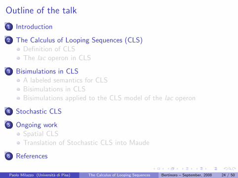
Outline of the talk

1 Introduction

2 The Calculus of Looping Sequences (CLS)Definition of CLSThe lac operon in CLS

3 Bisimulations in CLSA labeled semantics for CLSBisimulations in CLSBisimulations applied to the CLS model of the lac operon

4 Stochastic CLS

5 Ongoing workSpatial CLSTranslation of Stochastic CLS into Maude

6 References


The Calculus of Looping Sequences (CLS)

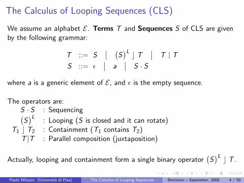
We assume an alphabet E . Terms T and Sequences S of CLS are givenby the following grammar:

T ::= S∣∣ (

S)L c T

∣∣ T | TS ::= ε

∣∣ a∣∣ S · S

where a is a generic element of E , and ε is the empty sequence.

The operators are:S · S : Sequencing(S)L

: Looping (S is closed and it can rotate)T1 c T2 : Containment (T1 contains T2)

T |T : Parallel composition (juxtaposition)

Actually, looping and containment form a single binary operator(S)L c T .


Examples of Terms

(i)(a · b · c)L c ε

(ii)(a · b · c)L c (d · e)L c ε

(iii)(a · b · c)L c (f · g | (d · e)L c ε)


Structural Congruence

The Structural Congruence relations ≡S and ≡T are the leastcongruence relations on sequences and on terms, respectively, satisfyingthe following rules:

S1 · (S2 · S3) ≡S (S1 · S2) · S3 S · ε ≡S ε · S ≡S S

T1 | T2 ≡T T2 | T1 T1 | (T2 | T3) ≡T (T1 | T2) | T3

T | ε ≡T T(S1 · S2

)L c T ≡T

(S2 · S1

)L c T

We write ≡ for ≡T .


CLS Patterns

Let us consider variables of three kinds:

term variables (X ,Y ,Z , . . .)

sequence variables (x , y , z , . . .)

element variables (x , y , z , . . .)

Patterns P and Sequence Patterns SP of CLS extend CLS terms andsequences with variables:

P ::= SP∣∣ (

SP)L c P

∣∣ P | P ∣∣ X

SP ::= ε∣∣ a

∣∣ SP · SP∣∣ x

∣∣ x

where a is a generic element of E , ε is the empty sequence, and x , x and Xare generic element, sequence and term variables

The structural congruence relation ≡ extends trivially to patterns


Rewrite Rules

A Rewrite Rule is a pair (P,P ′), denoted P 7→ P ′, where:

P,P ′ are patterns

variables in P ′ are a subset of those in P

A rule P 7→ P ′ can be applied to all terms that are instantiations of P.

Example: a · x · a 7→ b · x · bcan be applied to a · c · a (producing b · c · b)

cannot be applied to a · c · c · aExample:

(a · x)L c (b | X ) 7→ (

c · x)L c X

can be applied to(a · a · a)L c (b | b | (a)L c b)

the result is either(c · a · a)L c (b | (a)L c b) or(

a · a · a)L c (b | b | (c)L c ε)Paolo Milazzo (Universita di Pisa) The Calculus of Looping Sequences Bertinoro – September, 2008 8 / 50

Formal Semantics

Pσ denotes the term obtained by replacing any variable in T with thecorresponding term, sequence or element.

Σ is the set of all possible instantiations σ

Given a set of rewrite rules R, evolution of terms is described by thetransition system given by the least relation → satisfying

P 7→ P ′ ∈ R Pσ 6≡ ε σ ∈ Σ

Pσ → P ′σT → T ′

T | T ′′ → T ′ | T ′′T → T ′(

S)L c T → (

S)L c T ′

and closed under structural congruence ≡.


CLS modeling examples: the lac operon (1)

i p o z y a

DNA

mRNA

proteinslac Repressor beta-gal. permease transacet.

R

i p o z y a

R RNAPolime- rase

NO TRANSCRIPTION

a)

i p o z y a

R

RNAPolime- rase

TRANSCRIPTION

b)

LACTOSE



Ecoli ::=(m)L c (lacI · lacP · lacO · lacZ · lacY · lacA | polym)

Rules for DNA transcription/translation:

lacI · x 7→ lacI ′ · x | repr (R1)

polym | x · lacP · y 7→ x · PP · y (R2)

x · PP · lacO · y 7→ x · lacP · PO · y (R3)

x · PO · lacZ · y 7→ x · lacO · PZ · y (R4)

x · PZ · lacY · y 7→ x · lacZ · PY · y | betagal (R5)

x · PY · lacA 7→ x · lacY · PA | perm (R6)

x · PA 7→ x · lacA | transac | polym (R7)


Outline of the talk

1 Introduction



4 Stochastic CLS


6 References


Bisimulations

Bisimilarity is widely accepted as the finest extensional behavioralequivalence one may impose on systems.

Two systems are bisimilar if they can perform step by step the sameinteractions with the environment.

Properties of a system can be verified by assessing the bisimilaritywith a system known to enjoy them.

Bisimilarities need semantics based on labeled transition relationscapturing the potential interactions with the environment.

In process calculi, transitions are usually labeled with actions.

In CLS labels are contexts in which rules can be applied.


Labeled semantics

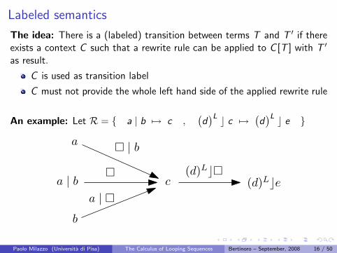
The idea: There is a (labeled) transition between terms T and T ′ if thereexists a context C such that a rewrite rule can be applied to C [T ] with T ′

as result.

C is used as transition label

C must not provide the whole left hand side of the applied rewrite rule

An example: Let R = { a | b 7→ c ,(d)L c c 7→ (

d)L c e }

a

a | b

b

c (d)Lce

� | b

(d)Lc��

a | �


Labeled semantics

Contexts C are given by the following grammar:

C ::= �∣∣ C | T ∣∣ T | C ∣∣ (

S)L c C

where T ∈ T and S ∈ S. Context � is called the empty context.

Given a set of rewrite rules R ⊆ <, the labeled semantics of CLS is thelabeled transition system given by the following inference rules:

(rule appl)P 7→ P ′ ∈ R C [T ′′] ≡ Pσ T ′′ 6≡ ε σ ∈ Σ C ∈ C

T ′′C−→ P ′σ

(cont)T

�−→ T ′(S)L c T

�−→ (S)L c T ′

(par)T

C−→ T ′ C ∈ CPT | T ′′ C−→ T ′ | T ′′

where CP are contexts that do not include(S)L c C and the dual version

of the (par) rule is omitted.


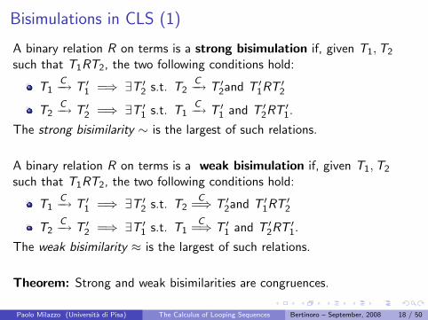
Bisimulations in CLS (1)

A binary relation R on terms is a strong bisimulation if, given T1,T2

such that T1RT2, the two following conditions hold:

T1C−→ T ′1 =⇒ ∃T ′2 s.t. T2

C−→ T ′2and T ′1RT ′2

T2C−→ T ′2 =⇒ ∃T ′1 s.t. T1

C−→ T ′1 and T ′2RT ′1.

The strong bisimilarity ∼ is the largest of such relations.

A binary relation R on terms is a weak bisimulation if, given T1,T2

such that T1RT2, the two following conditions hold:

T1C−→ T ′1 =⇒ ∃T ′2 s.t. T2

C=⇒ T ′2and T ′1RT ′2

T2C−→ T ′2 =⇒ ∃T ′1 s.t. T1

C=⇒ T ′1 and T ′2RT ′1.

The weak bisimilarity ≈ is the largest of such relations.

Theorem: Strong and weak bisimilarities are congruences.



Consider the following set of rewrite rules:

R = { a | b 7→ c , d | b 7→ e , e 7→ e , c 7→ e , f 7→ a }

We have that a ∼ d , because

a�|b−−→ c

�−→ e�−→ e

�−→ . . .

d�|b−−→ e

�−→ e�−→ . . .

and f ≈ d , because

f�−→ a

�|b−−→ c�−→ e

�−→ e�−→ . . .

On the other hand, f 6∼ e and f 6≈ e.

e�−→ e

�−→ e�−→ . . .



Let us consider systems (T ,R). . .

A binary relation R is a strong bisimulation on systems if, given(T1,R1) and (T2,R2) such that (T1,R1)R(T2,R2):

R1 : T1C−→ T ′1 =⇒ ∃T ′2 s.t. R2 : T2

C−→ T ′2 and (T ′1,R1)R(T ′2,R2)

R2 : T2C−→ T ′2 =⇒ ∃T ′1 s.t. R1 : T1

C−→ T ′1 and (R2,T′2)R(R1,T

′1).

The strong bisimilarity on systems ∼ is the largest of such relations.

A binary relation R is a weak bisimulation on systems if, given(T1,R1) and (T2,R2) such that (T1,R1)R(T2,R2):

R1 : T1C−→ T ′1 =⇒ ∃T ′2 s.t. R2 : T2

C=⇒ T ′2 and (T ′1,R1)R(T ′2,R2)

R2 : T2C−→ T ′2 =⇒ ∃T ′1 s.t. R1 : T1

C=⇒ T ′1 and (T ′2,R2)R(T ′1,R1)

The weak bisimilarity on systems ≈ is the largest of such relations.

Strong and weak bisimilarities on systems are NOT congruences.



Consider the following sets of rewrite rules

R1 = {a | b 7→ c} R2 = {a | d 7→ c , b | e 7→ c}

We have that 〈a,R1〉 ≈ 〈e,R2〉 because

R1 : a�|b−−→ c R2 : e

�|b−−→ c

and 〈b,R1〉 ≈ 〈d ,R2〉, because

R1 : b�|a−−→ c R2 : d

�|a−−→ c

but 〈a | b,R1〉 6≈ 〈e | d ,R2〉, because

R1 : a | b �−→ c R2 : e | d 6 �−→


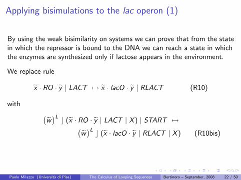
Applying bisimulations to the lac operon (1)

By using the weak bisimilarity on systems we can prove that from the statein which the repressor is bound to the DNA we can reach a state in whichthe enzymes are synthesized only if lactose appears in the environment.

We replace rule

x · RO · y | LACT 7→ x · lacO · y | RLACT (R10)

with (w)L c (x · RO · y | LACT | X ) | START 7→(

w)L c (x · lacO · y | RLACT | X ) (R10bis)


Outline of the talk

1 Introduction



4 Stochastic CLS


6 References


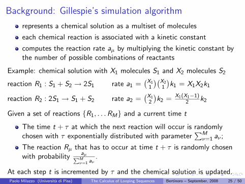
Background: Gillespie’s simulation algorithm

represents a chemical solution as a multiset of molecules

each chemical reaction is associated with a kinetic constant

computes the reaction rate aµ by multiplying the kinetic constant bythe number of possible combinations of reactants

Example: chemical solution with X1 molecules S1 and X2 molecules S2

reaction R1 : S1 + S2 → 2S1 rate a1 =(X1

1

)(X21

)k1 = X1X2k1

reaction R2 : 2S1 → S1 + S2 rate a2 =(X1

2

)k2 = X1(X1−1)

2 k2

Given a set of reactions {R1, . . .RM} and a current time t

The time t + τ at which the next reaction will occur is randomlychosen with τ exponentially distributed with parameter

∑Mν=1 aν ;

The reaction Rµ that has to occur at time t + τ is randomly chosenwith probability

aµPMν=1 aν

.

At each step t is incremented by τ and the chemical solution is updated.Paolo Milazzo (Universita di Pisa) The Calculus of Looping Sequences Bertinoro – September, 2008 25 / 50

Stochastic CLS (1)

Stochastic CLS incorporates Gillespie’s stochastic framework into thesemantics of CLS

Rewrite rules are enriched with kinetic constants

What is a reactant in Stochastic CLS?

A reactant combination is an occurrence (up to ≡) of a left hand sideof a rewrite rule

Example: The application rate of a | b k7→ c to a | a | a | b | b is 6k

Example: The application rate of(a · x)L c (b | X )

k7→ (c · x)L c X to(

a · a · a)L c (b | b) | (a · a)L c b is

6k , with(c · a · a)L c b | (a · a)L c b as result

+ 2k , with(a · a · a)L c (b | b) | (c · a)L c ε as result

= 8k


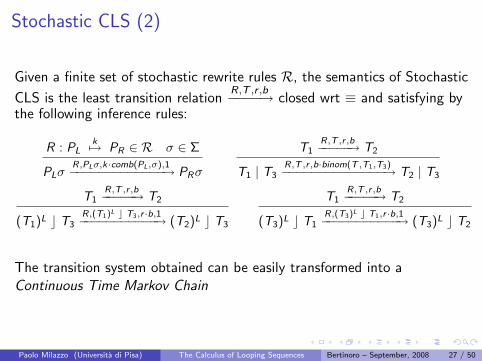
Stochastic CLS (2)

Given a finite set of stochastic rewrite rules R, the semantics of Stochastic

CLS is the least transition relationR,T ,r ,b−−−−→ closed wrt ≡ and satisfying by

the following inference rules:

R : PLk7→ PR ∈ R σ ∈ Σ

PLσR,PLσ,k·comb(PL,σ),1−−−−−−−−−−−−−→ PRσ

T1R,T ,r ,b−−−−−→ T2

T1 | T3R,T ,r ,b·binom(T ,T1,T3)−−−−−−−−−−−−−−→ T2 | T3

T1R,T ,r ,b−−−−−→ T2

(T1)L c T3R,(T1)L c T3,r ·b,1−−−−−−−−−−−→ (T2)L c T3

T1R,T ,r ,b−−−−−→ T2

(T3)L c T1R,(T3)L c T1,r ·b,1−−−−−−−−−−−→ (T3)L c T2

The transition system obtained can be easily transformed into aContinuous Time Markov Chain


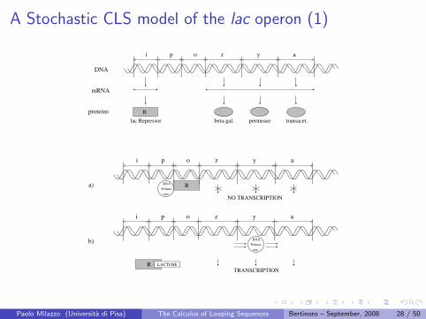
A Stochastic CLS model of the lac operon (1)

i p o z y a

DNA

mRNA

proteinslac Repressor beta-gal. permease transacet.

R

i p o z y a

R RNAPolime- rase

NO TRANSCRIPTION

a)

i p o z y a

R

RNAPolime- rase

TRANSCRIPTION

b)

LACTOSE


A Stochastic CLS model of the lac operon (3)

The behaviour of the three enzymes for lactose degradation:(x)L c (perm | X )

0.17→ (perm · x)L c X (S11)

LACT | (perm · x)L c X0.0017→ (

perm · x)L c (LACT |X ) (S12)

betagal | LACT0.0017→ betagal | GLU | GAL (S13)

Degradation of all the proteins and mRNA involved in the process:

perm0.0017→ ε (S14) betagal

0.0017→ ε (S15)

transac0.0017→ ε (S16) repr

0.0027→ ε (S17)

Irna0.017→ ε (S18) Rna

0.017→ ε (S19)

RLACT0.0027→ LACT (S20)


Simulation results (1)

0

10

20

30

40

50

0 500 1000 1500 2000 2500 3000 3500

Num

ber

of e

lem

ents

Time (sec)

betagalperm

perm on membrane

Production of enzymes in the absence of lactose(m)L c (lacI − A | 30× polym | 100× repr)



0

10

20

30

40

50

0 500 1000 1500 2000 2500 3000 3500

Num

ber

of e

lem

ents

Time (sec)

betagalperm

perm on membrane

Production of enzymes in the presence of lactose

100× LACT | (m)L c (lacI − A | 30× polym | 100× repr)



0

20

40

60

80

100

120

0 200 400 600 800 1000 1200 1400 1600 1800

Num

ber

of e

lem

ents

Time (sec)

LACT (env.)LACT (inside)

GLU

Degradation of lactose into glucose

100× LACT | (m)L c (lacI − A | 30× polym | 100× repr)


Outline of the talk

1 Introduction



4 Stochastic CLS


6 References


Spatial CLS

The spatial organization of elements may affect system dynamics

reaction-diffusion system

molecular crowding

We developed Spatial CLS by extending the Calculus of Looping Sequeces

Elements of Spatial CLS are spheres in a continuous space

the containment hierarchy is reflected in the spheres

elements can move autonomously

interactions can depend on the spatial information of elements(position, radius, ecc.)

rewrite rules are endowed with rates


Example of Spatial CLS term

T =(a)

[(1,2),m1],0.5| ((b · c · d)·,0.5)L[(4,3),m2],2

c (a)[(−1,0),m3],0.5


Rewrite rules

R : [ fc ] PLk7→ PR

k : reaction rate

fc : application constraints

takes into account the spatial information of involved elements(eg. position, radius, ecc.)

Example

[ dist(p, q) ≤ 5 ](a)

[p,f1],r1| (b)

[q,f2],r2

0.87→ (c)

[ p+q2,m],r3


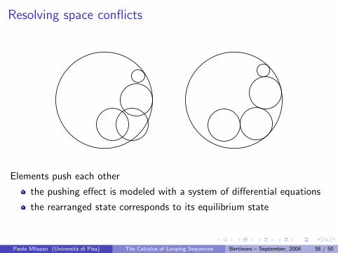
Resolving space conflicts

Elements push each other

the pushing effect is modeled with a system of differential equations

the rearranged state corresponds to its equilibrium state


Modeling cell proliferation

Initial state of the system:

T =(b)L·,50c (m)L

[(0,0),m1],10c (n)L c (cr · g1 · g2 · g3 | cr · g4 · g5)

(b)L·,50

: the available space(m)L

[(0,0),m1],10: the membrane of the cell(

n)L

: the nucleus

cr · . . . : the chromosomes


Rewrite rules modeling the behavior

R1 : [ r = 7 ](m)L

[p,f ],rc X

0.337→ (m)L

[p,f ],10c X

R2 : [ r = 10 ](m)L

[p,f ],rc X

0.257→ (m)L

[p,f ],14c X

R3 : [ r = 14 ](m)L

[p,f ],rc((

n)L c X

)0.57→ (m)L

[p,f ],rc((

ndup

)L c X)

R4 :(ndup

)L c (cr · x | X )0.1257→ (

ndup

)L c (2cr · x | X )

R5 :(ndup

)L c (2cr · x | 2cr · y)0.177→(

n)L c (cr · x | cr · y) | (n)L c (cr · x | cr · y)

R6 :(m)L

[(x ,y),f ],rc((

n)L c X | (n)L c Y

)17→(

m)L

[(x−5,y),f ],7c (n)L c X | (m)L

[(x+5,y),f ],7c (n)L c Y


Simulation

t = 0h


Simulation

t = 6h


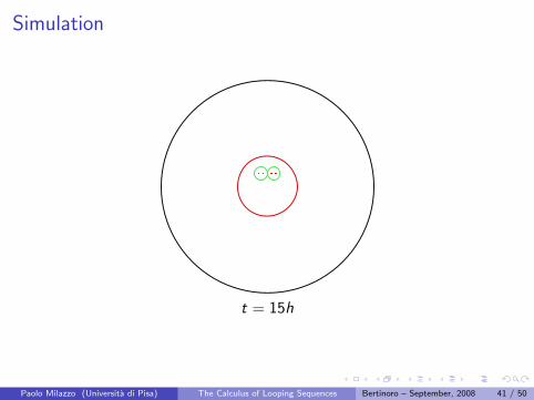
Simulation

t = 15h


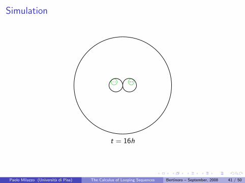
Simulation

t = 16h


Simulation

t = 20h


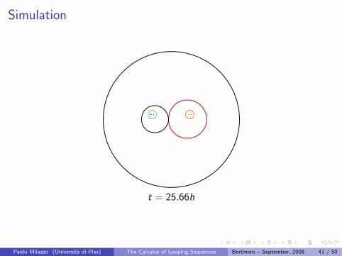
Simulation

t = 25.66h


Simulation

t = 88h


Simulation

t = 98h


Simulation

t = 102h


Simulation

t = 141h


Outline of the talk

1 Introduction



4 Stochastic CLS


6 References


A model checker for Stochastic CLS

As candidate model checkers we have considered:

PRISM

Murphi

PMaude

All of them are probabilistic/stochastic model checkers

PMaude is the most suitable

It uses a language based on rewrite rules (rewrite logic) that eases thetranslation of Stochastic CLS rules

Unfortunately, the model checking module of PMaude seems not to beavailable

a possible alternative: Real-Time Maude


Real-Time Maude

Maude is a specification language equipped with efficient analysis tools,which supports three modelling paradigms:

algebraic style (via equations)

rewrite logic (via rewrite rules)

object oriented (via classes and messages)

Real-Time Maude extends Maude with a notion of time

rewrite rule applications might consume (a fixed amount of) time

Real-Time Maude has two kinds of rules

istantaneous rules:crl [l] : t => t’ if cond

tick rules:crl [l] : t => t’ in time τ if cond


Translation of Stochastic CLS into Real-Time Maude

Real-Time Maude is not stochastic

we will include Gillespie’s simulation algorithm (slightly changed) inthe translation of Stochastic CLS models

it will be used to generate single executions of the model

Real-Time Maude analysis tools will be applied to the simulationresults

This is statistical model checking

we loose exhaustivity (properties are checked on a number of runs)

huge systems could be handled



T ::= S∣∣ (

S)L c T

∣∣ T | TS ::= ε

∣∣ a∣∣ S · S

(omod CLS ispr NATsorts Elem Seq Term Loopsubsorts Elem < Seq < Term

op empty : -> Seq [ctor]op . : Seq Seq -> Seq

[assoc gather (E e) id: empty ctor]op ‘[ ‘]LContains‘[ ‘] : Seq Term -> Term

[prec 41 gather (& &) ctor]op | : Term Term -> Term

[assoc comm prec 45 gather (E e) id: empty ctor]

endom)


Analysis example: statistical model checking

Initialisation of 100 stochastic simulations

rl [ initialise1 ] :< step : 0 >

=>< seed : random(1), step : 1 >

...

...rl [ initialise100 ] :< step : 0 >

=>< seed : random(100), step : 1 >


Analysis example: statistical model checking

Verification of properties espressed as LTL formulas. Some state formulas:

vanished(T) indicates that term T has vanished from the system,

IsLessThan(T,T’) indicates that the occurences of term T are less thanthe occurences of T’.

Starting with 4 x S1 and 4 x S2 we prove

that S2 will eventually disappear (i.e. 3vanished(S2))

that the amount of S2 will eventually become less than the amount ofS1 (i.e. 3IsLessThan(S2,S1))

(mc INIT({S1}4 | {S2}4) |=t <> vanished(S2) in time<=1 .)

Result Bool : true

(mc INIT({S1} 4 | {S2} 4) |=t <> IsLessThan(S2,S1) in time<=1 .)

Result Bool : true


ReferencesP. Milazzo, Formal Modeling in Systems Biology. A Theoretical Computer ScienceApproach, VDM Verlag Dr. Muller, Saarbruecken, 2008.

P. Milazzo. Qualitative and Quantitative Formal Modeling of Biological Systems,PhD Thesis, Universita di Pisa, 2007.

R. Barbuti, A. Maggiolo-Schettini, P. Milazzo and A. Troina. A Calculus ofLooping Sequences for Modelling Microbiological Systems. FundamentaInformaticae 72, 21-35, 2006.

R. Barbuti, A. Maggiolo-Schettini and P. Milazzo. Extending the Calculus ofLooping Sequences to Model Protein Interaction at the Domain Level. Symp. onBioinf. Research and Applic. (ISBRA’07), LNBI 4463, 638-649, Springer, 2007.

R. Barbuti, A. Maggiolo-Schettini, P. Milazzo and A. Troina. The Calculus ofLooping Sequences for Modeling Biological Membranes. Invited paper at the 8thWork. on Membrane Computing (WMC8), LNCS 4860, 54-76, Springer, 2007.

R. Barbuti, A. Maggiolo-Schettini, P. Milazzo and A. Troina. Bisimulations inCalculi Modelling Membranes. Formal Aspects of Computing 20, 351-377, 2008.

T.A. Basuki, A. Cerone, P. Milazzo. Translating Stochastic CLS into Maude.Work. on Membr. Computing and Biol. Inspired Calculi (MeCBIC’08), 2008.

R. Barbuti, A. Maggiolo-Schettini, P. Milazzo, P. Tiberi and A. Troina. StochasticCLS for the Modeling and Simulation of Biological Systems. Transaction onComputational Systems Biology, in press.


The Calculus of Looping Sequences - pdfs.semanticscholar.org fileThe Calculus of Looping Sequences...

Documents

Transcript of The Calculus of Looping Sequences - pdfs.semanticscholar.org fileThe Calculus of Looping Sequences...