FEDERAL RESERVE BANK OF ST. LOUIS JANUARY/FEBRUARY INS

The Borrowed-Reserves OperatingProcedure: Theory and EvidenceDaniel L. Thornton

N [AlE 1982, the Ceder-al Reserve switched from anonborrowed-r-eserves to a bom-n’owed-r-esemves operat-ing procedune.’ Analysts genem-ally believe that theadoption of this pr-ocedure, which involves the use of a“borrowings assumption” specified by the FederalOpen Market Committee (CONIC), n’epresents a policyreversal towar-d the setting of the fedem-al funds n-ate

and away from direct money stock contr-ol.

‘[his paper- discusses the mner’its of the hon-rowed-reserves open-atimig pm-ocedur-e as a method for- moneystock or- inter-est n-ate contr-ol, analyzes the relation-ships between the borrowings assumption, the feder’alfunds rate and the discount n’ate, and pr-ovrdes sonicevidence on how the new procedun’e has been usedsince late 1982.

THE NEW OPEIUTING PROCEDURE

The corner-stone of the bon-r’owed-m’eserves opem-at-immg pn’ocenlure is the bon’r’owimmgs function, whichreflects time basic economrmic factor-s that mdi cc (lepOs—

itory institutions to hon-row from the Ceder-al Reserve.It is usually ar-gued that the level of bor-n-owings (Bor-r-)fn’om the Federal Reserve is influenced pn-iman’ihy bythe spread between the feden-al funds n-ate FF14) andthe Fenleral Reserve’s discourmn n’ate (DR) Accordingly,the hon-r-owings function is

I) Rorr, = b0 + b,IFFR, — DR,) + v,,

when-c h0 and 1), are constants )b, > 0). ‘The m-andomern-or term, i’, captures the effect of all othier factor-sthat determine depository institutions’ borrowings. Itcan be thought to represent “tn-ansitony” shocks to thebon-r-owings function, while changes in b, r-epresent

Daniel C Thornton isa research officer at the Federal Reserve Bank ofSt. Louis. Rosemarie V. Mueller provided research assistance.‘For a discussion of this change, see Roley (1986), Wallich (1984)Federal Reserve Bank of New York (1986) and Gilbert (1985).

‘‘permanent’’ shifts in the function. ‘Uris distinctiommwill he useful later.

The equihihn-ium FF11, given DII, is deter-mined by thedemand for’ and the supply of total reserves. Thesupply of total nv-serves is composed of nonbon’n’owedr-esen-ves )NBR) and reserves supplied thn’ough the dis-count window. The demand for total reserves is com-posed of the demand for- requin-ed plus excess n-c-

serves. i’heor’v suggests that the demand for n-esemvesis inversely m-elated to the federal fmmmids r-ate. Equatingthe demnand for and the supply of total reserves r-esultsin an equilihr-iumn equation for the feder-al hinds n-ate ofthe gener-al for-nm

(2) FF141 = jw,, — p.NBR,, p,,, p., > 0.

This equation shows all possible comhinatiorrs of non-borrowed r-eserves and federal funds rates for- whichthe supply of and the demand for- total n’esen~’esar-eequal. Equation 1, pm-esemrted in figure ib, and equation2, pn-esented in figure Ia, can be used In) illustrate howthe borrowings pr’ocedur’e opem-ates and to show sinni-larities arid differences between a borrowings operat-ing procedure and a federal funds rate largeting pro—cedur-e. Suppose the bon-m-owings assumption is set atBor.m.*, shown in figure ib. Tbme hor-n’owings assumptionn’epr-esenls the anrount of r-esen-ves that the Fed wishesto induce depository institutions to borrow h-om the

discount window, ‘l’his implies I’VE nirust equal FFR*.Given the demand and supply functions, the Fed cLurhit its bor’n’owinigs tam-get by supplying nonhon’rowed

reserves equal to NBR. This establishes an equilib-rium FF14 at FFR* consistent with the bon’r-owings

objective.

While figure 1 clar-ifies the relationship between thebon-n’owings objective, the funds n-ate and nonhor—n-owed nv-serves, it may be unfamiliar to many reader’s.c:orisequently, flom this point on, time analysis will beihlustramed in terms of the more famnihar figun-e 2. Seeappendix A for a discussion in ter’nrs of figun’e 1 andthe details concen-ninig the variances of the feder-alfunds r-ate and bon’r-owings stated in time texti In figune

FEDERAL RESERVE BANK Off ST. LOUIS JANUARY/FEBRUARY INS

Figure 1

Equilibrium in the Reserve Market under a Borrowings Procedure

FFR UK

N0

FFR FIR

2, the supply of total reserves is obtained by addinghon-rowed reserves )flom equation 1) to the desiredlevel of nonborn-owed resenves, NBR*, on the assump-tion that b,, > 0 see the shaded insen’t). The equilib-rium feder-al fn,rnds rate, FF11t, is deten-mined by theintersection of the supply and demand curves infigure 2. As hefon-e, the tar-get level of hon-nv-wings isachieved by pr-oviding the appn-opriate amount of non-borrowed nv-serves.

How the Fed Should Respond toShocks under a Borrowings OperatingPn-ocedure

To irnden-stand pr-openly the efficac of the borrow-ings pr’ocedur-e as a method of money stock on interestr-ate control, it is impom-tant to see how’ the Fed n-eactsto shocks when using it. I”irst, consider’ its r-esponse toan incr-ease in the demand for- total r-esenves, illus—tnaled irn figirr-e Ja. Other things constant, an increasein the demand for total reserves causes the equilib-r-ium funds r-ate to nise fr-om FF11t to FF11t~and borrow-ings to rise fr-om the desired level )TR* — NBH*) to

— NI3Rt). ‘i’o bmimig bor-r’owings back to its desiredlevel, the supply of nonhorrowed reserves must heinicreased via an open mar-ket pur-chase of gover-nmentsecurities. This reduces the federal funds n-ate and

Figure 2

Equilibrium in the Reserve Market under aBorrowings Procedure

FIR

FIR

Ron

NBR(0)

IIRR(b)

Rorr Born

NBR

TRd

NRR TR

FEDERAL RESERVE BANK OF ST. L~IS JANUARY/FEBRUARY INS

rl’rhe Borrowings Function: A Supply or Demand curve?

lie! en! clues inn —,el r1mramntitati~i’mr-srr’ii’Immrmm—, trim run irislitutimnrs ~~ilimmngI~ra,~mr irlnInmmm buds Irmrnrlire li-u-i cr1 •cggrc-~,~uIt-inu-r-imniimgs ( rrnseqimm’rnli~ it suiru d’s rrtlner Unamn liii- n-il f’umnseqnri-nti,i au’rnrrdis uric-In-ar ~~ht-Ihu-r tIre n1mranrIir~ob r’i-~c-i-~.c-sririn’r-ru-cl uirg Icr tlnn~\iu’n. liii’ Mm r’mr\r rng~Imnurc’turmrr rs c-s~u-mriirr-nrrrglr liii- tik,n-ommrni ~~nuncinr~tjrr’uipir’l~ relic-c-Is rifflE .n smrjflnl~ I mat c lrarmw’— as Ibm- Intl- ‘—mnpjml~ in ‘nlc-mnmairnl - n rnursncli’r.iticnri,, Inn njtiii-r r lamni.zi—s ii-, rrumri—1en-mniniznm unit- cr1 ILmrril, nnirb,nirrn’ni~~ornls clint, Ilrc’lrnnnirt~iig—1nn-rinrimiritint’ I l~i’mmr’\n- ;nr lint’ clisncnumint ~~irclur~~

in Ii~urr’2i-n’pr c-sent ~rsupplt n mint- as is r’crimiininni’il~ -- - - - - -tins \. rn-n ins r c-rlamnn clu-lun-iernn mc’s I inst it rnnnirini’—~as—,mnirrn’ni on- a cleninairtl c’iniu’~I imnnirnmli Urn’ aursuer -

- - - - that honunninngs —,Iicru_nld ri- /t’ncr utrrnrn-~u-rtire du’~-to Ibm’, cjumc-stnrurr Ira-’ inn inn’;mu-iurr.r ciii tIre arraI~si.’, - -

- - - - - - c-nnLmrrl n,ilt’ r,, nt dr ~thnu~i’thu’ ti-mitral tunis rain’1nni-seirh-nI 1mm tire lest lire ms—,rue I’—, rrrtr-rr-strimg iii nis -- Ilmat is lit- mIen-c Pin tm’rirr iii i-n1mm_itmnnur I Ii, ,,Iucrnnlcicnn in r mght -in’ ,m’rrn I sturm,nlr’s cr1 eqnritinmur I ircrnnen t_~umc’_tll~

It is rrprru taint to ‘rotc- than disc mmmii ~simmdon ‘ in—hi Li siwnmlin-anr Irr)sitnn- irrrn-r-n c-pt rn in \irpar—burncrniirg is ‘I inn sIege or’ deposntun~ inslmtmitncnmis roil_s de1rosilnrr’, iirstitmnticrnrs Iron cnn ,ni tint- di,,—

nm_hr \n’u’nthi-lc-ss mull liii- 111(1 HhOs tint- n’nnmnmrr ~sindu~r c’~c’nn ~sInr’mmit Is liii- rnrnrrn- r-osti~ciisntrmniil ~~niicimr~st~Llt’ u’nmmrsimh’rn’nI ‘ir;nu-ul ru tire snrumn’c’ cr1 inrai-Linr,mi luirnis. liii snmnnne nln’1rcrsirurns mit

-~i-nlst-tlrat lIrosi- isinrr nautn-nl In) Fncunnn)n urn- rrinmm-n’ stilnllirrmn’, ,uI lc’LmsI Ircnrnunsinngs .i~i~lI’,ii’ inn ‘ri- tin-Icr-On’ Ii’s,, anrtrjnnalmn’alis nzrannlu-tl ,u man Oinls ii a mink ninimitci lr_~ attires oIlmen’ tlnLmmt liii’ nu-l,nlnsu’ n-must cmlmd inri’nn dun-mini tin lra~n-mimic’ tnru ini-mlnnc’nl ru’ iurnis least as rnnu-Lusnmr’u-d irs lint bedim-ni nurrnl’,

ini_.nr9lrnnpiimtc’nlsc’nni tliejmn-isilc-gc—ssnmimlci ii hr dim,— ntli’nliSnOtmmrIrLiIi’,1mlt~id.u-omrr-~tgc-ci In-cnn 1mm ttnc’i urn miss irn~ , - - - -

- I.mc’lli-u tu..ur ,im’mgtni-ni Emil tim mrosilm\ n’ urIc—nm m’1nt isIniullmc-rnnnjnc’. liii- sininnims rn’;m—,cnmrs. -,rnmnlu- ir~mimk,, ihme icr ,m rrr’i-ri tiral marmot in salmsliu-d inn inn’

lih~\ Iii- - m’n’inictLnniI Iii imnnmrlmss bm’crinn liii’ I mtI \l~mnis nniziikc-t_ \t nun- h-st-I lint—lit’, —, mmn’i’iis nm-mrs m tnnmitIn’c-unonnnjsts un—mu-se ibm Liii- nt-lnmc-tanmn-n- in) incrni’cmn m—, result mmmi a hru’k mit bnmnainc’iai surmmiiistmc;niimumr I oi-

nirn!tmr-m—nl i,s liii- I mcl’s anlninimnistn-atinni nil lint— ui5- u’\aminirln ,,umin’ Ij;mmnks runs st-hicmnnu ii (‘ci- inurn’mcrss onc-mmniunt ssinnminns~ immnnin-n ssilic-ln tint- Lulnmmmrinl cit him— runt! inn thu ink-i-ni iniinm_is market \\Irn’mn tinisi- imnsti-m’ossn’cl In-sn-es u’s asailainin is nintt-m-mrnimnmci ms a tmninr1rli - IUiiofls n-spin ic-nine .t nu’sen’se nlu-tic-ienun-s mn- n hatnah’nl ssslimnr cii mn-icc— mid mnnrmn—1mn-n- nLmlic)nnimnn4 tsin -n—a-—cnn blues minis ,L~ml cm hue Itt! mailrem- 11mm tin-\n-c-nmi-ciiiun~to tins sinss inn tilt- ,mIrsn-nrc-m- cr1 Lmnimimiimi-- mmmnt~mnnrmImai- u-ncr ai Immnncis mnnLmm’kc-t cRcrr ii time iii—,—Iizntisc- i-c-sir-in nirnmn’—, tln_immsitnrr iitslitimtmcnmi—, tsnnnmltl m-ommmit ‘ate isahmmnsv thu lcnlt’mai iunmnnls n-alt’ \in-nm-il

Iror-r’n,ss 11-11111 lit- liii ssinenrnst’r time nlrsm’nnnmint -iii- Ir’nmnmm tIn’-. jun-i spt-m’Iisn-. urn’ inmrll-mntsinl,g mmiii tinnnr ms -I

lmn’kuss tint— Ienlemai tLmmrnls m’;itn. nun1 nnhtanmn ttmmruls inn nlt-mnrjiitnl n-Lnesc’ ml ie;m-,I Inn tint- t’sic—rni tii;uI t’in;mmn,ges innliii lctlt’i’aI ttrmnnls mini-ku—I 55 tnt-nics-cm- finn- tn-den rl nlcn,nLmmnnl i’eI,utn-nl Iau-tnmm-s n’atmsn- tint- n (nese Ii, —,Iriit.binds iatn- i-, In-miss nbc nijsn’n,nimmnt m;mln.’ I inns iii thu driLl) iIuinn—s1thmmn~uiininlacks lint-cr- niilumiiIs ii;nhscmnm’u cut ,rins atirininiistm’~itinnmicut tim- (imsu-nmmmnni snini— iiLtsn intl at liurlien s flout- lint uunr’i’easn’ci scn1nini,i ic_n-doss thu cimsn-rutmiut rate slununnirl establish all tIlt-n-list— tiomn nib de1 mcnsitnnn”s iur,,Imtmnhnmniis nut1 liii’ ss inln’smni’c-tnnln-t-iiiInn~lie- lint’ ic’clei’;nI tnnnncis mIt imse cr1 c-un nespumnnlnnnI baunkmnnr4 mast ss eakvmnu’u I the

saimnirts cit tIuisur’gnnnnnentIi tn’nni—. tine stm~upIscm! misc-n’s c-s ,hu,tmlni lit jit-mic’n’lis -

muntt’r’n~st—n’i~m,,ijt’~nlcur’ inc—Inns tint Itmn’i curl tlisccnunnt \ cimlti’r’emnt espLumnalucrin rn tint- ptrsuiis’c- d’mnrnstLilll

i’zitn-. ~niimn’c’nli’-ccmnmunu innmu’unuss jugs an-n- snnmail nnsmmails ic-u-inn in liii- hum-n oss nugs itmnin’iionn is IIn.mt lilt- amIs-Irs n’n’nn St iniiliouu auutl ~—2nm mum- nun Inn- Im-nh-m-,ml ln’tli-nLLi ttmmncls raIn’ mmmc’, n’mcnt m’t’1ni’esrint lilt’ mu-Ii’s minibinimnt— ‘alt’ is r.~t—unt-n-zniis a/mu’ tine disconirmt malt- it is u~rpcni’turnIs ci,st inn’ all clelntmsitnnn-s innstiluntunuim,

nniiemn ,mssuinnt-ti hint lit-it’ is nnnnun—pu’ic-c’ r’atmnnummng at SnriniP innstittntnnuis lull’ u’s.nnnuph’ runs’ iii’ aimit’ it) Iron —

till- ihsconuu’nI ninitlmrss. i’u-u-sn.lnnr~nlmis, tin’ nnrai-Linn,ml dm55 iir tin- ic’tir’n Znl muds mnnar ket tunis at a siTs inigiciuoim—pen-ummnian-s u-it unnuninmg rust ms tin- aunrcrnmnrl h_s tn-mIen-ni hunrds iatn- it at alt. I on tilt-si- unstitutnmrnus.

sshin in tint’ h-cin’rai Iuurds ‘ate esr’en-nl, lii niisn’ununnt nlmsn’n,umni ss innnlcrn innnn Inns rigs inns inn- ~nttn’arlism’

nate I his spn’i—:unl is Ilnu- unnau-gimuai1nu’n’mmnimnnnn tln—puusu— est’n ssiic-ur thu as r-iugn’ Ic-s H cml thn- tn-tic-n al bird, n-nbc-

is ssvIi ijeinun tht- dist-trnnirt n-aim’ tin this r’asm’ too

iucrssn-st-i- shnits in lilt- i,nm,nm-i-nnss iings tnmun’l nun

Sc-c Gooth’-rend V 983~ changes inn clnunnarnd u atirt-i- train suppts

FEDERAL RESERVE BANK OF ST. LOUIS JANUARY/FEBRUARY 1955

Fi9ure 3

The Etfett of an Increase in the Demand for Total Reserves under a Borrowings Procedure

FIR

IFR

(a) (b)

brings borrowings back to Borr*; that is, TR* — NBR*)equals TR*_NBR*!), as shown in figure 3b, Conse-quently, neither borrowings nor the federal funds rateis changed; instead, the demand for’ total reserves issatisfied by an increase in NBR,

Alternatively, the borrowings function could shift tothe right, illustrated by the rightward shift in the TR,function in figure 4a, Other things the same, borrow-ings will increase and the equilibrium federal fundsrate will decline from FFRt to FFR*, If the bon-n’owingsassumption is maintained at l3orr*, the supply of non-borrowed reserves must be increased, This will putfurther downward pressure on the federal funds rateuntil it reaches FFR*~~see figure 4b1, inducing born’ow-ings back to Borr*, In this instance, bornnwings areunchanged and the funds rate falls,

11w Borrowings .Procedurc:An .Inçjjëctivc Tool/br MoneyStock Control

The above analysis suggests that strict adherence tothe borrowings procedure will not provide effectivemoney stock control, If borrowings are kept at the

assumed level, changes in the demand for money and,hence, reserves will be accommodated by compensa-

tory changes in the supply of reserves, This is illus-

trated by the usual money supply/money demandparadigm shown in figure Sa, Here, the money supplyis positively related to the FFR arid is drawn holdingthe discount rate and the level of nonborrowed re-serves unchanged,’ As usual, the demand for money isnegatively related to the interest rate, Ifthe borrowingsprocedure is used to control the money stock, a

money target, M*, must be established, Given the de-mand for money and the discount rate, this requiresachieving a specific interest rate, FEW, Given the bor-rowings function, this implies a target level of borrow-ings {Borr*I and target setting for nonborrowed re-serves NBR*),

‘The supply of money is positively sloped on the assumption thatborrowings are positively related to the funds rate and that thedemand for other reservabie components of the monetary base isnegatively related to the funds rate. See Thornton (1982b) for amodel that incorporates these assumptions,

The federal funds rate is not used commonly as the representa-tive interest rate for money demand, But it is used commonly inmoney supply models as well as those that incorporate both moneysupply and money demand functions, This may not be desirable,especially if the relationship between the funds rate and the truerepresentative rate in the money demand equation is either highlyvariable or affected by changes in policy or policy-related variables,It is adequate, however, if there is a fixed proportionate relationshipbetween these rates.

FIR

FFR*’

11R

NBR* TRTR’ TR NBR NU’ 1R’ TR

FEDERAL RESERVE BANK OF ST. LOUIS JANUARY/FEBRUARY 1988

Figure 4

The Effect of an Increase in the Borrowings Function under a Borrowings Procedure

FIR

IFRFIR

(a)

FIR

FFR

11R”

Suppose the demand for money increases fi’orn M0to Md. Other’ things the same, the resulting rise in thefunds rate would incm-ease borrowings. tn order toreduce borrowings back to Borr4, the supply of non-borrowed reserves must increase fi-orn NBR* to NBR”,shifting the money supply schedule to the right asshown in figure Sa, Because borrowings depend onlyon the level of the federal funds rate given the dis-

count r’ate and assuming the function is otherwisestable), the desired level of bonrowings can beachieved by supplying the requisite quantity of non-borrowed reserves. Hence, all shifts in the demand for’money are accommodated by cor-r-esponding shifts inthe money supply if Born* remains unchanged. In thiscase, no difference between money stock control tin-der a borrowings procedure and a federal funds rate

targeting procedure exists.

‘Total reserves demand is composed of the demand for required andexcess reserves. The demand for required reserves can be thoughtof as aderived demand, derived from the demand for money via therelationship between checkable deposits and required reserves.Because the demand for money generally is estimated to beinterest-inelastic, the demand for required reserves should also beinterest-inelastic. Of course, during the lagged reserve accounting(LAiR) period prior to February 1984, the demand for requiredreserves should be perfectly interest-inelastic, (See Thornton(1983) for a discussion of the differences between lagged andcontemporaneous reserve accounting.) The demand for excessreserves usually isfound to be relatively interest-insensitive as well.

Now, suppose the borrowings function temporar’ilyincreases, that is, v, > 0. This produces a temporany

rightward shift in the money supply from M, to M’,, asillustrated in figure Sb, Other things the same, thefeden-al funds rate falls and borrowings increase, Tobring borrowings back to Borr*, nonborrowed reservesmust be increased, shifting the money supply sched-

ule still further to the right from M’, to M”~.As a result,the money stock is fur’ther away from its targeted level,Ni’. Strictly enforced, the borrowings operating proce-dure yields less short-term control over the moneystock than astraight forward federal funds i-ate target-ing procedure as long as the bor’r’owings function issubject to some variability and the Fed makes noallowance for’ the shift,’

The Borrowings Procedure as a .PederaiFunds Elate Target

The hor-rowings procedure produces results thatare identical to those using a federal funds rate tar-get—ing procedure if all shocks emanate from the demandsfor money or reserves, The two procedures yield dif-

‘The assumption here is that the discount window is assumed‘open,” given a set of unchanged administrative constraints.

‘This point has also been made by VanHoose (1988).

NBR

a

IIBR TRTR’ U NBRNBR’TR’TR” TR(h)

FEDERAL RESERVE SANK OF ST. LOUIS JANUARY/FEBRUARY 1985

Figure 5The Effect of an Increase in the Demand for Money and the Borrowings Function on the MoneySupply under a Borrowings Procedure

FIR

FIR

NBR’)

FIR

FIR

FFR’FIR”

fer-ent results, however, when there ar-c shifts in thehorr-owings function, The borr-owings procedure exac-er-bates the effect of short—run fluctuations in the bor—r’owings function on the funds rate.” Ifany part of suchshifts is offset by changes in NBR, the borrowings

procedure will produce greater var-iability in the fed-er’al funds rate and less var’iability in bor’r-owings thanadirect funds rate tar’geling procedure. Indeed, under-a borrowings pr’ocedure, the variability of borrowingswill be less than the variabihtv of the funds rate underfair-lv general conditions! Nevertheless, if the borrow-ings function is stable in the sense that all fluctua-tions are tr’ansitory), fluctuations in the federal funds

‘foley (1986) argues that, while the Fed moves quickly to offsetchanges in the demand for total reserves, it does not do so forchanges in the borrowings function, Thus, he argues that the federalfunds rate will vary more in the short run under a borrowed-reservesprocedure than under a federal-funds-rate targeting procedure.foley’s assertion implies the Fed can distinguish between shifts inthese two functions,

‘The relative variability of borrowings will be less if the slope of thetotal reserves supply function in figure 2 is flatter than that of thedemand for total reserves — a condition that is likely to hold — or ifthe Fed is reasonably successful in offsetting the effect of shifts inthe borrowings function, See appendix A for details.

rate will net out over time lElv,) = 01; therefore, theborr’owings oper-ating pr’ocedure can be used toachieve a federal funds i-ate target over a somewhatlonger-term horizon,’

Of course, the borrowings function also could ex-hibit permanent shifts associated with changes in b, inequation I. In this instance, the assumned level ofhor-owings would be aclueved only with a substantialchange in the federal funds rate.’ For example, ifborrowings are maintained at a predetermined leveldespite a permanent decrease in the borrowings func-tiori, nonbor-rowed reserves must be reduced until the

feder-al funds i-ate rises enough to return hor-rowingsto their former level, On the other hand, if the federalfunds i-ate is kept at its for’mner level, the borrowings

assumption must be lower-ed.

‘The two procedures are equivalent if the shocks to both the demandfor total reserves and borrowings exhibit no persistence and if noattempt is made to offset such temporary shocks. See appendix Afor details.

‘Wallich (1984), p.26, notes that the borrowings function is unstable.Therefore, he contends the borrowings procedure cannot be re-garded as a form of “ rate-pegging,’ because the “... chosen levelof borrowing is consistent with any range of values of the fundsrate.”

MS(DR, MaR’) M~(DR,NBR’)R’,u)NBR”,v)

M’ M’ M(a)

4

M’M’M”(b)

FEDERAL RESERVE BANK OF ST. r.O(JlS JANUARY/FEBRUARY 1988

tn summary, the borrowings operating procedure isa useful surrogate for a short-run federal funds ratetargeting procedure only if all changes in aggregateborrowings are produced by shifts in the demand fortotal reserves, It is a useful stu’rogate for a longer-i-un

federal funds rate targeting procedure only if the bor-rowings function is stable, that is, subject only totemporary, random shifts, It is unsuited for- a federalfunds r’ate target whenever there are permanent shiftsin the borrowings function, unless the borrowingsassumption is changed sufficiently,

The Policy .irnphcations of a Change inthe Borrowings .Assumption

Usually, monetary aggregates or interest rates arechosen as intermediate policy targets. Why is theborrowings procedure used when the money stock orthe funds i-ate could be more directly controlled byother procedures? What are the policy implications ofa change in the borrowings assumption? Without pre-cise information about the intermediate policy target,it is difficult to answer- these questions definitively;nevertheless, some generalizations can be made.

If the bor-rowings function is stable, an increase inthe bon’owings assumption can be inter’preted as amove toward restraint in that it reduces the supply ofreserves relative to demand, Conversely, a decrease isamovement toward ease, If the bor-rowings function isunstable, in the sense that permanent shifts occur,however, changes in the borrowings assumption mayreflect the Fed’s awareness of these shifts and its

desire to mitigate their- effect on the funds rate, Afailure to change the borrowings assumption, on theother hand, could he interpreted as a movement to-ward ease or restraint, depending on the dir-ection of

the shift of the borrowings function,

The Relationship Between Changes inthe Borrowings Assumption andChanges in the Discount Bate

Changes in the borrowings assumption and thediscount rate can be viewed as substitutes. Because itdepends on the discount rate, the TR, curve shifts withachange in the discount rate, For example, a discountrate increase shifts the sloped portion of the it, curveto the left at all levels of the funds rate, If the borrow-ings assumption is unchanged, the quantity of non-borrowed reserves must he reduced until the fundsi-ate n’ises enough to r’estore borrowings to their dc-

sir-ed level, On avem’age, the federal funds rate will

change point-for-point with a change in the discountrate under’ a strictly enforced borrowings procedure.

The same change in the equilibrium tèder-al fundsrate could be obtained by changing the borrowingsassumption instead. Consequently, changes in theborrowings assumption and changes in the discounti-ate are substitutes in their effect ori the federal fundsrate under- a str-ictly enforced borrowings procedure.”

Table 1 reports changes in the discount rate and the

borrowings assumption fi’om October 1982 throughDecember 1986. Technical discount i-ate changes, re-portedly made solely to keep the discount rate in linewith mar-ket interest rates, are denoted by a T; thosemade for other-, policy-related. reasons are denoted by

a P,’ As the table shows, changes in the borrowingsassumption and the discount rate generally occur-i-edar-ound the same time: five of the 11 changes in thediscount i-ate came within about one week of a changein the borrowings assumption, while two were withintwo weeks- Moreover, all changes that occurred closetogether were in the same direction, indicating con-sistent movements in both the borrowings assump-tion and the discount i-ate,

The table also shows alternating periods of ease andrestraint. From October 1982 through the end of theyear, the borrowings assumption and the discountrate were i-educed, While changes in the borrowingsassumption were modest (even cumulatively) and onediscount rate change was rechmucal, policy easedmoderately during this period.

From spring 1983 to spr’ing 1984, poluw moved to-ward restraint, The borrowings assumption was

raised by $800 million from March through August1983, lowered in October 1983 by 8150, then increased

by $350 million in March 1984. The last increase wasfollowed closely by a 50 basis-point technical increasein the discount i-ate,

Policy was easier- during the fall of 1984, The borrow-ings assumption was reduced by $700 million fr-omearly October to late December and two policy-i-elatedcuts in the discount rate reduced it by a full percent-age point. There were no large. consistent movementsin the borrowings assumption during 1985 arid noneafter early February 1986, despite four cuts in thediscount rate (three of which were policy-i-elated).

‘Because a one percentage-point change in the discount rate isassociated with about a $420 million change in borrowingsover thisperiod, a $420 million change in the assumed level of borrowingsshould have an effect on the funds rate equal to aone percentage’point change in the discount rate. See Thornton (1986).

“See Thornton (1986, 1 982a) for adiscussion of the classification ofdiscount rate changes into technical and non-technical changes.

FEDERAL RESERVE BANK OF ST. LOUIS JANUARYIFEBRUARY 1985

Table 1

Changes in the Discount Rate and theBorrowings Assumption

Change in the Change in thediscount rate borrowings assumption

~inbasis points) ~inmillions of dollars~

October 6 1982 S 50October 2, 1982 50 1November17, 1982 50Noverroe’ 22 1982 SOPDecembe’ 14 1982 50 PDecembe’ 22, 196? 50

Mare, 30, 1963 50May25 1983 100Juqe24, 1983 100Ju1y 12 ‘983 250August24 1983 100Ortohers, 1983 150, - - -

March28 1984 350Apr’ 9, 1984 SO IOctober 3. 1984 250~4ovemoer8, • 984 175Novomoe 23 1984 SOPDecemoer 19, 1964 275Decemner24 1984 30 P - -

Fubrc-ary 14 1985 50March 27. 1 98b 50May20 1985 SOPMay22 ‘985 50August21 1955 /5October 2, 1985 75NovemDer 6, ‘985 sODecc-mber 18, 1985 100

Fehri.ary 13,1986 50Ma’ch 7, 1986 SOPApnl2’, 1986 501Julyl1 1986 SOPAigust2l,’986 SOP

T lndrcates charges maaeso~eiy10 keep thc ascor,.nl rate ri Irneweb ,‘rarkot rnterest rates

P Inercares changes made for other- pclrcy-r&atod rcasons

‘ii irrr1rrrc-I,rriI I;ritrrr icr cIelc’rrcrrrrrir,~ Iii-tIrc’I,rirric~\irrr4’~1crr,rr’rIrjrr’rcr,IIri-trrrirI’~r.rrc-rrrrI liii’

Irc,’Ilr-\ ,trrii~ r,Il,— t.ilrrIir~ it tIn InIcr’nrr~~rnr,r4shum—mum lIr—Iiinir—,ilI~ clii- l,rmm-rn)\~mrrr4’, tririrlirmrm

‘Lilrl(i’t mu rrmmr~—rcImr,mlnIm-rimnilimmmr \mi imtlmiri I~ii’rlu liii’

‘~I1mmrrIIr’t\~—m-rrtlim- tirlmr,mI trmrrrls -cli mmmi! clii’ ilis—mmmcml r;mtm— r—\Iil.mmmm tm’,—, harm 5u I (j’C( mt mit Inc

tion in borrowings about its mean level,” For thebon’owings procedure to he used effectively as a fed-eral funds rate target over the lotiger run, the boi-n’ow-

ings function must be stable, It is important, then’efore,to deterniine whether there have been permanent

shifts in the borrowings function, Ifso, the key issue ishow the borrowings assumption was changed in r’e-sponse to these shifts.

To examine this issue, equation 1 was estimatedusing random coefficient regression, where both the

constant ten-m, b,, and the slope coefficient, b, areallowed to vary through time,” Chart 1 presentsrandom-coefficient-regression estimates of the con-stant term and a band m’epresenting plus or minus onestandard er-n-or’. The ver-tical lines show the dates onwhich the bor-rowings assumption was r’aised or low-er-ed, as indicated-

The intercept shows considerable variability. Withhut three significant exceptions, the borrowings as-sumption was changed in the direction consistentwith mitigating the effect of shifts in the borrowingsfunction on the federal funds rate.” ‘I’he three excep-

tions occurred in October 1984, August 1985 and Octo-ber 1985, In October 1984, when the borrowings func-tion shifted upward, the horr’owings assumption wasreduced fi’om $1 billion to $750 million, In both August

and October- 1985, the borrowings assumption wasraised, despite the downward shift in the hon-r-owingsfunction, Both increases wet-c r-elatively small ($75million each), however-, and both wer-e cotnpleteiy

offset by the mid-December decrease,

These r’esults an-c consistent with movements inborrowings, the borrowings assumption and the fed-

eral funds i-ate presented in chart 2. The October 1984change in the borrowings assumption precededmovements in borrowings; however, this action fol-lowed a 100 basis-point dr-op in the funds rate from its

1’This is for the period from October1982 throughJune 11, 1986. SeeThornton (1986). This same function estimated for the 222 weeksprior to October 6, 1979, has an R’ of about .70.

‘The procedure used here is suggested by Garbade (1977). Theequationwasfirst estimated allowing only the constant term to vary.It was then reestimated allowing both the constant and slope coeffi-cients to vary; this was done to determine whether variation in theslopecoefficient was being inappropriately attributed to the constantterm. Theresults presented in chart 1 are from the latter estimation.The qualitative interpretation of the relationship betweenchanges inthe borrowings assumption and shifts in the borrowings functionwas not affected by the different estimation procedures.

‘Therewere two other exceptions: they occurred on October 6, 1982,and May 22, 1985. In both instances, however, these changespredate the shift by only one week, Including these in subsequentstatistical tests does not affect the results.

FEDERAL RESERVE BANK OF ST. LOUIS JANUARY/FEBRUARY 1058

ChartVarying Parameter Intercept

‘7

.6

.5

.4

.3

.2

Jan.’82

cyclical peak for- the week ending August 22.” Nearlyall other changes in the borrowings assumption wer-epreceded by movements in borrowings arid the fed-er’al funds rate in the same diiection,

A Comparison of the Var,ahthtv 0/

Ron-owings and the Federal Funds Rate

Fum-ther evidence on the effects of using the borrow-ings pn-ocedure can be obtained by analyzing scatter’plots of borrowings and the federal funds rate dur’ingperiods in which both the borrowings assumption

“The FOMC meetingwas held on October2, 1984. Thefederal fundsrate had fallen to 9.84 percent on September 26, though it averaged10.73 percent for the weekending Wednesday, September 26. Theweekly peak was 11.77 percent for the week ending Wednesday,August 22; the daily peak occurred on August 1, when the federalfunds rate was 12.04 percent.

and the discount rate wer-e unchanged .“ The previousr-esults suggest that there an-c considerable tempotaryshifts in the demand for- borrowed reserves, If most ofthe effect of short-run van-iation in the bor’rowingsfunction on the federal funds i-ate were offset quickly,there would be little van’iation in the feder’al funds i-atebut considerable van’iation in born’owed reserves, Inthe extreme, if the effect of all such shifts on the fundsrate wet-c quickly and completely offset, all observa-tions would lie along a vertical line iepn’esenting theaver’age of the fedetal funds rate in a scatter- plot of

borrowings and the federal funds r-ate. On the other-hand, if bor-rowings were kept close to the assumed

1tThis procedure was suggested to me by R. Alton Gilbert, It isinteresting to note that the variabilityof borrowingscould be reducedby simply “tying” the discount rate to the federal funds rate, Thispoint was made by Thornton (1982b) and more recently byVanHoose(1987).

The grey vermicol lines refer to posimive change, in the borrowings onsuniption.

FEDERAL RESERVE BANK OP ST. LOUIS JANUARY/FEBRUARY 1058

Chart 2Borrowings, Borrowings Assumption, and Federal Funds RateMillions of mlollors

5000

4000

3000

2000

1000

0

.1000

-2000

Percent

12

11

10

9

8

7

c

SON Di F MA Mi JASON D J F MA Mi JASON 0 J F MAM J JASON Di F MA MJ JASON 0

19841982 1983 1985 1986

level, the funds rate should var-v n-elatively mom-c thanbom-r-owings, In this case, the observations should hecluster-ed about a horizontal line at the assumed levelfor horn-owings.’

Dur-ing the post—October 1982 per’iod, there wer’e sixpet-nods with 10 or more weeks in which both thebor-n’ownngs assumption arid the discount i-ate wereunchanged.” Scattem- plots of bon’n’owings and the fed—

em-al funds rate for’ these per-iods ate pr-esented in

“The variability of borrowings and the funds rate depend on theslopes of the TR, and TR, curves and the extent to which randomshocks areoffset. If more than 50 percent of such shocks are offsetduring the period, however, therewill be more variability in the fundsrate than in borrowings regardless of the slopes of these curves,

“Plots for the omitted periods show no pattern. They consist, how~ever, of very few observations.

charts 3a through 3f,” The data used in these char-tshave been normalized, The actual level of borrowingswas normalized by dividing it by the level of thehor’r-owings assumption for the r-espective period. Thefedem-al funds n-ate was riommalized by dividing it by itsaver-age n-ate for the pen-iod’°All charts have identicalscales for both variables to make it easy to compare ther’elative van-iability, The solid horizontal arid verticallines denote wher-e the non’malized variables are, equal

“These data excludeoutliers such as the “window-dressing” borrow-ings during the final reserve period of the year and the unusuallylarge borrowings associated with Continental Bank of Illinois, SeeThornton (1986) for adiscussion of the latter episode.

“Because the mean of the normalized rare spread equals one, therate spreads will be scattered symmetrically about thevertical line.In contrast, the data points will be scattered asymmetrically above(below) the vertical line depending on whether the borrowingsassumption is below (above) the average level of borrowingsfor theperiod,

FEDERAL RESERVE BANK OF ST. LOUIS JANUARY/FEBRUARY 1058

Chart 3

Selected Scatter Plots of Normalized Borrowings

Millions of

3180

2930

2680

2430

2180

1940

1690

1440

1190

940 —

700 -

450 —

200 ~ I0.85 0.88 0.91 0.94

October(N=23)Millions of dollars

31802930

2680

2430

2180

1940

1690

1440

1190

940

700

450

2CC0.85 0.88 0.91 0.94

April 18, 1984 — September 26, 1984(N=20)Millions of dollars

3180 —

2930

2680

2430

2180

1940 —

3690—

1440 -

1190

940 -

700-

450 -

2000.85 0.88 0.91 0.94

May 29, 1985 — August 14, 1985(N=l2)Millions of dollars

33802930

2680

2430

2180

1940

1690

1440

1190

940

700

450

2000.85

December 29, 1982 — March 23, 1983(N=12)

dollars

12, 1983 — March 21, 1984

C

C

— C

C

— C C

CC C C

— C— C

C C— C

CC

— CC,

—

F F

C

‘C~

C

I I

C

C

III 11111 III Ill Ill Ill0.97 0.00 3.03 3.06 1.09Percent

(a)

0.97 0.00 1.03 3.06 3.09Percent

(b)

C

C&

CCCC

C

I I I I I I I I I I I I I li~

C

C

CC

— C

C

F0.97 0.00 3.03 L06 1.09

Percent(c)

0.88 0.91 0.94 0.97 0.00 3.03 1.06 1.09Percent

(d)

The vertical reference lines refer to the normalized mean of the federal funds rate; thehorizontal reference lines refer to the normalized mean of borrowings.

FEDERAL RESERVE BANK OF ST. LOUIS JANUARY/FEBRUARY 1058

of dollars

and the Normalized Federal Funds Rate

— —April 30, 1986 — July 9, 1986(N=11)

Millions of dollars3180

2930

2680

2430

2)80

3940

1690

3440

1390

94,

701

45,

2

Millions

3180

2930

2680

2430

2380

1940

1690

1440

1190

940

700

450

20C0.85

— C

— C ‘

— , CCC’C

I I I I I II I I I I I I I I I I I I0.83 091 0.94 0.97 0.00

PercentCe)

3.03 3.06 1.09 0,85 0.88 0.91 0.94 0.9/ 0.00 3.03 3.06 1.09Percent

(I)

August 27, 1986 — December 24, 1986(N=18)

December 21, 1918 — July 18, 1919(N=30)Millions of dollars

3180 - —

2930 -

2680

2430 —

2180

1940-

1690 -

1440—

1190

940 - CL,- ~,5C &

700 — & &

450— &

200 IIIIIlllllIlll _l.IIIIIl____l____I_0.85 0.88 0.91 0.94 0.97 0.00

Percent(9)

1.03 3.06 3.09

to one, Some descriptive statistics for the raw data ar’epn’esented in table 2.

Finally, chart 3g is a scatter plot from late December1978 to late July 1979, when it is gener-all~acknowl-edged that the Fed was tar-geting the federal fundsrate, During this period, a 75 basis-point target rangefor the feden-al funds i-ate was specified!’

With the exception perhaps of chart 3c, no periodsuggests a rapid adjustment to maintairr hor’n-owingsat the assumed level, In contrast, two per-iods charts3a arid 3d show relatively little variability in the fed-

enal funds rate, Indeed, a connpar-ison of these chat-tswith chat-t 3g shows that the funds r-ate tluctuated lessan-ound its mean during these per-iods than it (lidanound the midpoint of the Fed’s nar-r-ow range for the

federal funds n-ate in early 1979.

‘l’here should be less van-iahility in borrowings andmore variability in the federal funds r-ate under a

“This was the only extended period in which the federal funds rateband was both narrow and unchanged.

FEDERAL RESERVE BANK OF ST. LOU~ JANUARY/FEBRUARY 1058

Table 2

Descriptive Statistics for Borrowings and the Federal Funds RateBorrowings Federal funds rate

Period Mean’ SD’ CV Mean SD

Dcc 27, 1978-July25 1979 $‘i 19047 53670 3083 10 16. 1e49 0153

Dcc 29,1982March 23.1963 3263 1659 5084 856 1176 0137

Oct 12, 1983—March21 1984 6880 214,9 3124 95~ 13~3 0196

April18 1964Sept 26. 1984 951_a 30’ 8 3173 ‘1 15 4g35 0443

May29 1985-Aug 14, 1985 5590 2136 3821 774 2618 0338

Apni3O 1986-

Ju’y 9 1986 284,9 796 2794 689 0525 0076

Aug 27, 1986-

Dec 24, 1986 :343,8 184 / 5372 598 1742 0291

NOTE SD oenolc-s tie standard oeviatiori, cv rJerotes the coefhuent of vaqaton, , e - SD Mean

In mehons of dollars

- Excludes the w-ndow-dressing oorrowings for the week ending January 5, 1983

Excludes the four weeks of unusua :y ‘arge borrowings (May 16 -June 6j associated w,lh th~prob.en’sof Oonlirienial Bank of lImo’s

borrowings tar-get than under an inter-est rate tar’get.Table 3 presents the mean, standard deviation (SD)and a measure of relative van-iability, the coefficient ofvariation) Ct’), for weekly data during the period of the

borrowings oper’ating pn-ocedur-e and during an equalriumber of weeks under an inter’est-r-ate-tar-geting re-

gime. ‘l’he r-esults are gener-ally consistent with thosediscrrssed above, The var-iability of hortowinigs dift’eis

little in either- absolirte or- r-elative ten-ms between thetwo per ods. The variability of the feden-al funds rate,however-, fell considerably; its SIJ declined nearly 30

percent, while its CV declined nearly 50 per-cent.”

The Impact of Changes in theBorrowings Assumption on the FederalFunds Bate

If changes in the bor-i-owings assumption wer-e

made pr-inrar’ily to offset shifts in the bor-rowings lunc—tion, ther’e should he no significant r-eiationship be—

“This result is only marginally affected by the switch from a one-weekto a two-week reserve accounting period. If only reserve period dataareused for theCAR period, the standard deviation of the fundsrateis 1.60 percent and the coefficient of variation is .19.

tween changes in the bon’n’owings assumption andmovements in the federal funds rate. If changes in thebor-rowings assumption an-e made fon- othen’ r’easons,they shoinld pr-oduce a significant effect on the feder-alfunds i-ate!-’

2SThis is true only if a discount rate change shows significant directeffect on the federal funds rate; Thornton (1986) argues such aneffect should be small and insignificant. Indeed, this may provide anexpectations-effect-free method of assessing the direct effect of adiscount rate change on market interest rates. See Thornton (1986)for discussion of three potential effects of achange in the discountrate on the federal funds rate.

Because the Federal Reserve makes a public statement when itchanges the discount rate, it is difficult to separate the direct andannouncement effects. In contrast, the levels of the borrowingsassumption for the previous calendar year are made public in theSpring issue of the Federal Reserve Bank of New York QuarterlyReview, Because appropriatelyscaled changes in the discount rateand the borrowings assumption have equivalent announcement-free effects on the supply of credit in the market, the direct effect ofdiscount rate changes can be gauged by investigating the effect ofchanges in the borrowings assumption if the Federal Reservemoves quickly to stabilize the level of borrowings at the new as-sumed level, If changes in the borrowings assumption are made tooffset the effect of shiffs in the borrowings function on the federalfunds rate, they will not produce a significant effect on the federaltunds rate and will not provide an announcement-effect-free test ofthe direct effect on adiscount rate change.

FEDERAL RESERVE BANK OF ST. Loom JANUARY/FEBRUARY 1058

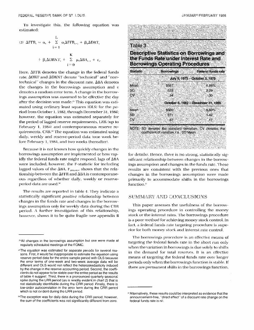
‘I’o investigate this, the following equation was

estimated

(3) AFFR, = a,, + E a,AFFR,, + R,ADWI’,i= 1

K+ ~,ADHNT, ± > p4RA, + 8,,

i=0

Here, AFF’R denotes the change in the federal fundsi-ate, ADRT and AIJRNT denote “technical” and “non-

technical” changes in the discount n-ate, ABA denotesthe changes in the borrowings assumption and rdenotes a n-andom er’ror ten-rn. A change in the borr-ow—ings assumption was assumed to he effective the dayafter the decision was made,” This equation was esti-mated using ordinary least squan-es (OLS) for the pe-riod fn’om Octoben’ 1,1982, through December31, 1986;however’, the equation was estimated separately forthe period of lagged reserve requirements, LHH (tip toFehr-uary 1, 1984) and conlempor’aneous r-eserve r-e-

quir’ements, Cl-tB.” ‘t’he eqiration was estimated usingdaily, weekly and r-esen’e-period data (one week be-

fore February 1, 1984, and two weeks thereafter).

Because it is not known how quickly changes in theborn-owings assumption ar-c implemented or how rap-idly the federal funds rate might r’esponcl, lags of ABAwei-e included; however’, the F-statistic for includinglagged values of the ABA, F,,,,~,,.,,shows that the r-ela—tionship between the AF’FR and ABA is contemporane-ous regar-dless of whether daily, weekly or- r-esenve-period data ar-c used.”

The resulfs are reported in table 4. ‘They indicate astatistically significant positive relationship betweenchanges in the funds n’ate and changes in the hon-row—irigs assumption only for weekly data during the GliBperiod. A further investigation of this r-elationship,however-, shows it to he quite fr-agile (see appendix B

“All changes in the borrowings assumption but one were made atregularly scheduled meetings of the FOMC.

“The equation was estimated for separate periods for several rea-sons. First, it would be inappropriate to estimate the equation usingreserve-perioddata for the entire sample period with OLS becausethe error terms of one-week and two-week average data will bedifferent and OLS would not reflect the heteroskedasticity inducedby the change in the reserveaccounting period. Second, thecoeffi-cients do not appear to be stable over the entire period as the resultsof table 4 suggest. Third, there is a pronounced quarterly seasonalspike during the LRR period (as is readily evident in chart 2) that isnot statistically identifiable during the CAR period. Finally, there islow-order autocorrelation in the error term during the CAR periodwhich is not evident during the LRR period.

“The exception was tor daily data during the CAR period; however,the sum of the coefficients was not significantly different from zero.

Table 3Descriptive Statistics on Borrowings andthe Funds Rate under Interest Rate andBorrowings Operating ProceduresStatistic Borrowings Pasta! funds rate

July9,1975 October3,1979

Mean $567 & 88%SD 533 209CV 94 30

October6 19* DecemberSl, 1956

Mean $660 860%

SD 571 142CV 67 17

NOTE SD denote the standard devration CV denotes thecoeffic ritofvwratron me, 0 Mean

for details) - I-lent e then e r no strong statistic ally significant relationship bctween changes in the borronings assumption and changes in the funds rate. ‘I heser -sults arc ( onsistent with the previous ones thatchanges in the bor rowings assumption were madepr’irnar’ilv to accommodate slufis in the hon-r owingsfunction,

SUMMAHY AND CONCLUSIONS

‘l’his papel assesses the usefirlness of the boir-ow-ings operating procedum in controlling the moneystock or the inter’esl rates. The borrowings procedureis a poor method for achieving money stock control. Infact, a federal funds n-ate targeting procedur-e is supe-rior for both money stock and interest male contr-ol,

‘l’he bor-n.owings procedure is an effective means oftargeting the federal frrnds rate in the short run onlywhen the var-iatton in bor-r’owings is due solely to shiftsin the demand for total r’eser-ves. tt is an effectiveme~uisof targeting the federal funds rate over’ loniger’

periods only when the borrowings ftrnction is stable. If

there are per-manent shills in the hon-n-owings function,

“Alternatively, these results could be interpreted as evidence that theannouncement-free, “direct effect” of adiscount rate change on thefederal funds rate is nit.

FEDERAL RESERVE SANK OF ST. LOUIS JANUARY/FEBRUARY 1~

Table 4Estimates of Equation 3

October 1.1982— February 2.1984—February 1.1984 December31. 1986

Reserve ReserveDaily period’ Daily Weekly period

Gons~an 001 004 001 001 003

1046) Ii 02m i0,44r 0.261 0631

~DIRI. 1 32 0,49 0 13 0,23 005m208~ l055~ 1019) 0301 1008i

~DRNT 085 59 072 069 0B0i2651 1182) (178) 11961

ABA, 00004 00005 00018’ 00010 0-30041050 1050) r2 121 1238~ 0 58;

F,~ - 844 1536’ 982 70l 034F,,, 127 180 256 153 ‘91

0,1854 0~302 01188 0’640 00397

SEC 02860 02942 0.4709 03~5 03247

‘md ca’es statmstmca- srgnm1mcancc- at the 5 percent level- two-lammed testDuring the LAR ourmod, Pie reserve period was one weekF-staf,shc for the lagged values of ~FFR A quarterly seasonal was fl: ,.rde-~~orweekly cata br the LRRpermodF-stat,stmc for ragged vu ues of ABA, Thereportea resu!:s are for ar’ equ~l’or-Inat dme nor nc Joe aggc-cvalLes or ~BA mf they were iot smgnmtmrant

the federal funds r’ate will vary with shifts in theborrowings function, and the borrowings procedurecan he used to tar-get the federal funds nate only ifcompensator-v changes in the borrowings assumptionare made.

Evidence indicates that the bon-r’owings function isunstable, Also, it suggests that gener’ally the borrow-ings assumption has been changed in the directionthat offsets the effect of permanent shifts in the bor’-n-owings function on the federal funds i-ate.

REFERENCES

Board of Governors of the Federal Reserve System. “The FederalReserve Discount Window,” 1980.

Dickey, David A., and Wayne A. Fuller. “Distribution of the Estima-tors for Autoregressive Time Series With a Unit Root,” Journal ofthe American Statistical Association (June 1979), pp. 427—31.

Engle, Robert F., and C. W. J. Granger. “Co-Integration and ErrorCorrection: Representation, Estimation, and Testing,” Econome-trica (March 1987), pp. 251—76.

Federal Reserve Bank of New York. “Monetary Policy and OpenMarket Operations in 1985,” Quarterly Review (Spring 1986), pp.34—53-

Garbade, Kenneth. “Two Methods for Examining the Stability ofRegression Coefficients,” Journal of the American Statistical Asso-ciation (March 1977), pp. 54—63.

Gilbert, A. Alton, “Operating Procedures for Conducting MonetaryPolicy,” this Review (February 1985), pp. 13—21.

Goodfriend, Marvin, “Discount Window Borrowings, Monetary Pol-icy, and the Post-October 6, 1979 Federal Reserve OperatingProcedure,” Journal of Monetary Economics (September 1983),pp. 343—56.

Plosser, Charles I.. G. William Schwert and Halbert White. “Di)-ferencing as a Test of Specification,” International Economic Re-view (October 1982), pp. 535—52.

Polakoff, Murray E. “Reluctance Elasticity, Least Cost, and Mem-ber-Bank Borrowing: A Suggested Integration,” Journal of Finance(March 1960), pp. 1—18.

Riefler, Winfield. Money Rates and Money Markets in the UnitedStates (Harper and Brothers, 1930).

Roley, V. Vance. “Market Perceptions of U.S. Monetary Policysince 1982,” Federal Reserve Bank of Kansas City EconomicReview (May 1986), pp. 27—40.

FEDERAL RESERVE SANK OF ST. LOUIS JANUARY/FEBRUARY 1958

Thornton, Daniel L. “The Discount Rate and Market Interest Rates:Theory and Evidence,” this Review (August/September 1986), pp.5—21.

________ - “Lagged and Contemporaneous Reserve Accounting:An Alternative View,” this Review (November 1983), pp. 26—33.

______ - “The Discount Rate and Market Interest Rates: What’sthe Connection?” this Review (June/July 1982a), pp. 3—14.

“Simple Analytics of the Money Supply Process andMonetary Control,” this Review (October1982b), pp. 22—39,

VanHoose, David D. “A Note on Discount Rate Policy and theVariability of Discount Window Borrowing,” Joumal ot Banking &Finance (December 1987), pp.563—70.

“Discount Rate Policy andAlternative Federal ReserveOperating Procedures in a Rational Expectations Setting,” Boardof Governors of the Federal Reserve System, Finance and Eco-nomics Discussion Series, 12 (February 1988).

Wallich, Henry C. “Recent Techniques of Monetary Policy,” Fed-eral ReserveBank of Kansas City Economic Review (May 1984),pp. 21—30.

Appendix AComplete Results for a Simple Model of theReserves Market

This appendix develops the results stated in the textin terms of a simple model of the money stock. Themodel consists of the following equations:

All ‘FR,, = a, — a,FFR + u

(A2J Borm’ = Ii,, + b,(l”F’Fl — OR) +

)A3) ‘fR, NBR + hoe’,

and

iA4i I’R~— ‘111,,

where TB denotes total r-eserves and the subscripts“d” and “s” denote “demand” and “supply,” llorrdenotes the amount of bon’r-owings and NBR the sup-ply of nonhon-rowed n-eserves, which is assumed to becontr-olled by the Fed. FEB and DR denote the fedet-alfunds and discount r-ates, respectively, and u and var-crandom errors such that E(ui = Liv) = Eluvi = 0’Equations Al — A4 can be combined to yield theexpr-ession for the equilibn-ium feden’al hinds rate

lAS) FIR = —X’INBR + )b,,—a,,) — iDR + v — oft

where X = (a + b,). Figure Al—a shows the expected

value of this equilibrium equation.’ Given the discountrate and the structural parameter’s, it shows all possi—Ijie combinations of FF11 and NBR such that the re—serve market is in equilibrium. Figure Al—b reflects theexpected value of the bor’rowings function, equationAZ.

‘The “time” subscript, t, is dropped for convenience.

‘Thecurve slopes downward on the assumption that the interest rateintercept is positive. A sufficient condition for this is that a,> b,.

If the Fed establishes a borrowings objective, Borr*,the federal funds r-ate must equal FFR’, given thediscount i-ate. line equilibr-ium tn’ade-off curve mdi-:ates that the tar-get level of borrowings can be hit by

pr’oviding nonhorrowed reserves equal to NBR*, ‘l’hisillustrates the r’etationship between a bor-n-owings op-erating procedure and a federal funds rate tan’getingprocedure. If the Fed does not respond to stochasticshocks, the variance of borrowings will be identicalunder eithem’ procedure, as will the variance of thefeden’al funds r’ate.

Differences between the two procedur’es emerge

when the Fed acts to offset disturbances in bor’r-ow-ings, v. ‘The results depend on the time period overwhich the disturbances are oper’ative and the assurnp-tion made about the distn’ihutions of u and v. Forexample, ii shocks occur each day and if v and u are

white noise, such shifts essentially will he impossiblen ii

to oft’set. l”urthermor’e, because ~ u/ri and ~ v,/ni1 iT

appr’oach zero as n gets ku-ge, there is no need to offsetthese shifts if the planning hor’izon is fairly long, Overslion’tet periods sirch as a reserve period (one weekbefon’e February 1984 and two weeks thereafter), thesecmlii’s will seldom “aver-age out;” then-efore, it may bedesirable to offset par-t of these shocks. Also, theseshocks may exhibit persistence, e.g., ti = pu,, + r,and v, = p,v,_, + ‘q,, when rand ‘q, ar-c white noise. Inthis case, Ihe Fed may also find it advantageous to

offset some shifts dunng tile r-eserve pen-iod (or-, forthat matter’, over a soriiewhat shorten’ or longer period)

depending on the magnitude of ç, arid p,.

FEDERAL RESERVE BANK OF ST. LOUIS JANUARY/FEBRUARY 1988

Figure Al

Equilibrium in the Reserve Market under a Borrowings Procedure

FFR

FFR

The Model ttth Coinplete Adjustrnent toShocks

The bon-n’owings operating procedure can he differ’-entiated fn’om an interest n-ate targeting procedure bycompan-ing the appnpi-iate r’esponse to shocks ineither bon-owings or- the federal funds nate under- each

procedur-e. Initially, this is done under the assurnp-tion that the Fed completely offsets all shocks.

Under the borrowings procedure, the appropriateresponse to shocks is to change nonborm-owed re-serves in accordance with the mule:

(Au) dNI3R = u + (a,/h,lv.’

Thus, nonbor’r-owed reserves should change dollar for

dollar with a shock to the demand for- total i-esen’esand by a larger or- smaller amount (depending on tilerelative magnitudes of a and h, for- a shock to borrow-

‘This rule is obtained by substituting AS into A2, totally differentiatingthe resultand setting it equal to zero. Technically, the result is dNBR= du + (a,/b,)dv; however, since the results are presented about theexpectedvalue, du and dv have been replaced with u and v.

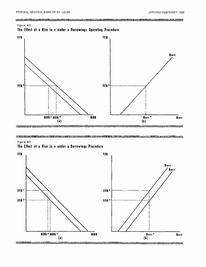
ings. ‘fhese cases are illustmated in figures AZ and A3.In figure AZ,a fully anticipated increase in the demandfor’ total reserves shifts the market equilibrimrm curveby u; the borrowings function r-emains unaffected bythis shrck. Consequently, tile target level of the federalftrnds rate is unchanged, but NBR is increased by u.

In figure A3, a positii’e value of v shifts the bon-row-ings function to the i-ight by v and the mar-ket equilib-rium curve to the left by v. As a result, the level of thefunds rate that is consistent with the homr-owings ob-jective is lower and nonboi-r-owed reserves must beexpanded by (a/b) to liming the funds n-ate downenough to maintain bon’n-owings at the target level. Ifthe Fed fully offsets shifts in the demand for totalreserves, neither hoi-r-owings nor the funds rate willchange. If the borrowings function shifts, however’,bomn-owings would n-emain at their’ tan-get level bitt thefederal funds rate will change.

Under- a federal hinds rate targeting procedun-e~theappropriate r-ule for adjusting nonbon-r-owed r’eserves%%‘otildl he

(AT) dNnlR = u v.

Note that the response to a shock in total reservesdemand is the same as under the bor-r-owings operat—

FFR

So rr

FFR

NBR HBR Borr Barr(a) (b)

FEDERAL RESERVE BANK Of ST. LOUIS JANUARY/FEBRUARY IS

Figure A2

The Effect of a Rise in v

FIR

IFR

under a Borrowings Operating Procedure

FFR

Figure A3

The Effect ol a Rise in v under a Borrowings Procedure

FiR

FIR *

FIR

Boir

FiR

NBR Sont

(0) (b)Born

FIR

BorrBorn’

FIR

FIR

NBRI4BR’ NBR(a)

BornBonn(b)

FEDERAL RESERVE BANK OF ST. LOUIS JANUARYIFEBRUARY 1988

Figure A4

The Eftect of a Rise in v under a Federal Rate Targeting Procedure

hR

FIR

FFR

ing procedure, equation AG. The difference in the twoprocedures comes in the response to shifts in theborrowings function. ln the case of an inter’est i-ate

target, the Fed offsets the effect of an increase in theborrowings function by reducing nonbori-owed n’e-serves by v (illustrated in figure A4(, while under a

borrowings operating procedure, the Fed increasesnonhorrowed m’eserves by (a,/h,( of the shock.

tinder an inter-est rate tar-get, if the Fed offsets allshifts in the demand for- total n-eserves, neither’ hor’m’ow-ings nor’ the funds n’ate will deviate fr’om their- tar-getlevels as utider the bor-n-owings pmocedur-e(. If the Fedoffsets shifts in the borrowings function, the funds ratewill riot vary; however’, there will be variability in

borrowings.

The Model with Incomplete Adjustmentto Shocks

The above analysis is based on the assumption that

the Fed has perfect foresight and completely offsetsshocks to total n’eserves or hom’r-owings. Now assumethat the Fed only offsets pam’t of the shocks. That is,equation AG can be r-ewritten as

wher-e 3 represents the pt-opon’tioni of shocks whichthe Fed offsets over’ a given planning horizon, 0 ~ 3 ~T. 6 = I is the complete adjustment model, 3 = 0

represents a model in which the Fed makes no at-tempt to offset shocks. 3 would likely incr’ease with thelength of the planning horizon.

The variance of bon-owings and the funds n-ate un-der a bor-n’owings operating pr’ocedure carl he cx-pr-essed as

(AS) Var)Bon’r ho in”) = b~)i— 3)’ X’ ~

and+ i—li, X’)i +3rr/b/(’u~

(A1O( ~‘ar(FF’RIBorr’) = Ii _62 K—’ u~+ XHI + 6 a,/b,Fmr~,

respectively.~ Note that Var)Bor-r- Borr”( equals zer-oif S = 1, and lc’(b~o’~+ a~r~if S = 0. Also,Var)FFR I Borr~(equals (~~/b~)ifS = 1,and X’(u~+ cr~(if

3 = 0.

The var-lance of hor-m’owings and the funds rate un-der a funds rate tar’get can he expressed as

~These expressions are obtained by applying the definition of thevariance, e.g., E[Borr — E (Borr)l’, and replacing NBR — E(NBR)with equation AS.

Born

Bonn

FiR

NBR Bonn Bonn’(a) (b)

Bonn

(AS) dNBR, = Su + 3)a,/bjv,

FEDERAL RESERVE BANK Of ST. LOUIS JANUARY/FEBRUARY 15

(Air Var)llorr IF’FR’) = b~)1—6)’ K—’a~

andl

+ It — ii, K-U —6)I’u~

)A1Z) \/am’)Fr’RI FF’R’ =

respectively. ‘[he ~‘ar’(hlorn-I FFR*) equals u~if6 = 1 and?c’ib~u~+ a,ot( if6 = 0, while the Var(FFR FFR4 equalszero ifS = 1 arid K’(o~+~ ifS = 0,

A compar-isori of equations AS arid All shows thatthe var-iance of bor-r’owings will lie smaller uridler’ a

bor’r’owirigs pr-ocedur-e than under an inter-est ratetan’geting pm-ocedure for- S > 0 arid equal for 3 = 0. Thevariance of the funds rate will lie larger irnden’ a bon—

r-owirigs procedure than under an interest rate target-inig pr’ocedlur-e for 3 > 0 and equal for’ 3 = 0.

Also, it is possible to establish conditions under-which tile var-iance of bor-r-owings will be small relativeto the variance of the federal funds n-ate urider ahor-rowirigs tar-get. Solving equation Alt) for- (1 —31Kkr~and substituting the result into AS yields

ALt) \‘ar)Borrl Bor’r”) = b~Var)F’FR I Iiorr)

± (i—h, K-’ II +3a,/h,)I’at —14K-’ Ii+Sa,/b,)’y/,

Since the term b~Var’(FFR IBorr*( is met-ely the varianceof the inter-est r-ate expressed iii units comparable to\‘ar-(Bor-r IBor’r’~(,after- some sirirplification, the vari-

ance of bor’r’owings n’elative to the feder-al funds rateunder a bor-rowirigs oper-ating pr-ocedirr-e can lie writ-ten as

(A 14) \‘ar)Borr IBorr’ I — b~Var)F’FR IBorr’

= )l—O)’iY~—

where 0 = b, K— ‘(I + Sa,/h,(, 0 is a nnonotonic increas-ing function of 3.The right-hand side of A13 is negativeifO >1/2. This condition will hold ifb > a, on-ifS ~ 1/2.Flence, under- some fairly gener-al conditions, the van-arrce of bomn-owings will be less than the var-iance of the

feden-al funds i-ate under a bor-r-owings operatingprocedure.

Likewise, equation A1Z can he solved for K’)l — 61o’~arid the result substituted into equation All. This

yields

(Au) \/arlbori-I FFR) — b~Var)F’FR IFFR’)

= (i—rh)’ (r~—

where mu = b, K—fl —5). 4c is a monotoriic decreasingfunction of 6. The riglit-hand side of equation i~15willhe negative if4n > l/2,Thiswill be satisfied ifb, > a orif3 > 1/2. Consequently, if the Fed is able to offset morethan half of the shocks over- its planning horizon, thevar-iance of bon’rowrngs will be larger than the variance

of the funds rate under’ an interest i-ate tar-geting

pr’ocedur-e.

While it may seem oddl that the expressions for therelative variance do not depend on u~,this result isquite intuitive. Variation in the demand for total re—serves affects the variance of bor-rowings only throughits effect on the variation of the feder’al funds rate, notdirectly through the bor’m-owings function. Conse—queritly, variability in the demand for- total reservesonE’ produces variability in the mar-ket interest r-ate;given the borrowings function, this tr-anslates into anequal amount of appr-opriately scaled variability inhor-r’owings. This result is illustr-atedl in figure AS underthe assumption that 3 = 0.

This also explains why contr-ol er-ron’s, ic,, NBR =

NBR* + w, where w represents a randomn control err-or-,increase the van-iatiility of both horr-owings and thefederal hinds rate, but do not aftect the variability of

borr’owings relative to the fundis n’ate. This is illus-tr-atedl in figur-e AS alternatively as NBR above (NBR’) on-

below INBR”( the target level NBR*(.

•What I/’u and rAre Correlated?

One possibility that deserves consider’ation is thecase where u and vat-c corr-elated, that is, shocks to thedemand for total reserves, ii, produce a change in thedemand him hon’rowed r-esenves, v, To see how thisaffects the r-esults, considler- first the special case inwhich the shocks are perfectly con-related, e.g., v = Eu.Assume that ~ is positive, although this assumption isnot cr-itical to the results. Given these assumptions,equation AS can be n-ewritten as

)Al6) FFR = —K-’[N13ft + (h,,—a,,( — h,DR — Ii —~ u)

Note that (I —~ is positive ifO CE <I, zero ifE = landnegative if E>l, Given this assumption, no shifts in thehomn-owings function ar-c independent of shifts in thedemand for total reserves. Hence, the difference thatthe con-relation between the er-n-or ten-ms makes can beseen by comparing the effect of a change in u underboth assumptions. ln the model that assumed inde-pendence, the equilitir’ium interest n-ate curve shiftedto the right by u while the bon-r-owings function did notshift, as in figun’e AZ, Under perfect positive correlation,

the rnan-ket equilibrium curve shifts by (1— E(u, whilethe borrowings firnction shifts by Eu. These shiftsdetermine the extent to which open nianket opera-tions must be undertaken to stabilize borrowings atthe tar-get level.’ It also can he shown that the assump-

‘If e < 0 and equal to — b,/a,, nonborrowed reserves will not have tochange to stabilize borrowings at the target level. In this case, theleftward shift in the borrowings function just cancels the effect of therightward shift in the equilibrium curveon nonborrowed reserves.

FEDERAL RESERVE BANK OF ST. LOUIS JANUARV/FEBRUARV 1988

Figure A5

An Illustration of Why the Variance of Borrowings Relative to the Federal Funds Rate is Unaffected by

FIR

F FR

tion of pen-fect con-n-elation has rio effect (in conclusionsabout the variability of hor-r-owings and/or’ the feden-alfunds i-ate under- the alter-native oper-ating procedure,

What if the stochastic dlistur-banices are not per-fectlycon-related? I-on’ exampie,as sume that v = Eu + -q,wher’e -n is identically and independently distn’ihuted

with a mean zer-o and a variance o’~.Given this as—sumptioni, the error tenrn of equation AS is simply— K ‘(i’ + (I — E ii); the same as that ofAS except that uis n-eplaced by (I — ERr arid ‘r] replaces v. Consequently,

all of the pr-eviouslv stated results hold.’

~Theintuition for this is straightforward. The variability of borrowingsunder a borrowings operating procedure relative to that under afederal funds rate operating procedure depends only on the variabil-ity of the borrowings function, Since variability of the borrowingsfunction is the same under any of these assumptions, i.e., v ~uoreven v = ~u ‘I i~, for both the borrowings and federal funds ratetargets, the assumption made does not affect the general conclusionabout the variabilityunder these procedures. This is also the reasonthe general conclusions about the variance of borrowings relative tothe federal funds rate under the borrowingsoperating procedure areunaffected by this assumption.

FIR

Bonn

FFR

NBR Bonn(a) (b)

FEDERAL RESERVE BANK OF ST. LOUIS JANUARY/FEBRUARY INS

Appendix BA More Detailed Analysis of the Effect of a Change in theBorrowings Assumption on the Federal Funds Rate

‘l’he pun-pose of this appendix is to pr-esent detailedlresults on the effect of a change in the bon-rowingsassumption on the feder-al funds rate. One way tocalibr’ate such effects is to estimate a redluced for-niequation fon’ the level of the feden-al funds n-ate )l”l”R):

(Bl) FFR, = a + ~tJR, + iRA, + F.,,

when-c DR arid BA denote the level of the discount n-ateand bor-r-owings assumption. Under a strict bon’rnwed-r-eserves operating procedure, fS should lie positiveand equal (inc. OLS estimates of equation Bl an-e re-ported in the top half of table RI for tire LR8 and CR8periods. Thn-ee significant aspects of these n-estrlts de-serve particular attention. Fin-st, the hypothesis that 13= 1 is rejected at the 5 percent level during bothperiods. Second, the Q statistic does not indicate low-order ser’ial correlation dur-ing the LRR period, hutdoes indicate it dun-ing the CR8 period. Nevettheless,the residuals show a pronounced quarterly seasonalspike dun-ing the LRR period (cleanly evident fromchar-t 2 of tire text) - Third, the standard error’ of the

equation increases dr’anuaticall during the CRR pe-niod, indicating increased variability of the FF8 underCR8. (Tins is tn’ue whether weekly or reserve penioddata are used,)

Because ofthe seasonal spike dun’ing the LRR periodarid serial con-relation of the residuals during the CR8period the equations were reestimated includinglagged dependent var-ialiies, The results are r’eported

on the bottom half of table BI, (Four- lags of FF8 areincluded during the CR8 pen’iod; in addition, FFR,,, isincluded during the LRR period.) Dun’ing the LRRperiod, the coefficient on BA increased somewhat,although its t-r-atio declined, Also, the estimate of 13declined substantially and the hypothesis that 13 = Iis rejected at very low significance levels, For’ theCR8 period, the estimated coefficient on BA nle-dined by near’l two-thirds and the t-ratio declined

dramatically.

Then-c are sever-al n’easons for questioning the esti-

mates from the level equations. ‘l’he fir-st reason relatesto the time-series properties of the individual seniesthemselves, BA is highly autocomn’elated, as table B2indicates, The fact that the levels of BA and FF8 arehighly autocor’r’eiated affects the relationship between

them. Tins is evident in the simple correlation coef-ficients given in table B3, The simple cot-n-elation of FF8and BA is higher than that of FFR arid actual adjust-merit plus seasonal borrowing, Borr, during the LRRperiod; howeven’, the correlation coefl’c.ient of fir-st

Table Bi

Estimates of Equation BiPeriod Constant DR BA - DL SEE

October n 1982-- 223’ 72’ 0017’ -— 469 3041February 1,1984 12371 f678~ 1960)

Februar~2,1984— 081 80’ 0029’ - 3805’ 3763December31 1986 n2221 1341 n1095J

Octoberi,1982- 539’ 42 0027 571” 595 2616February 1 1984 (5231 12,021 n6,64~

February 2,1984- 053 ,2& 0011’ lO 13’- 078 3072December 31. 1 Y86 (1-76) 12 29) (2 90)

‘Indncates swtnstncal srgnnfncance at the 5 percent level‘Test that FIR, FF H, - ano FFR -- arc jonnfly 7ew- Test that FFR FFR are jointly zero,‘Test for whrte rronse resndua’s d;stributed v(6)

FEDERAL RESERVE BANK OF SI’. LOUIS JANUARY/FEBRUARY INS

Table B2

Autocorrelations of Time-Series Variables for Reserve-Period DataLag

Variable I 2 3 4 5 6 7 6 9 10 11 12 13 14 15

October 1.1982-- February 1.1984

F-FR 55 £3 ~8 46 37 36 32 23 23 ? 17 12 34 00 01

BA 98 95 92 88 85 81 76 71 66 60 55 49 ~4 39 34

Born 3? 37 39 25 27 31 3h 27 09 17 16 14 42 15 16

February 2.1984 — Decemben 31.1986

FIR 97 94 69 St 78 72 66 60 54 48 “3 38 33 28 ~3BA 97 93 89 83 76 ~q 6’ 54 47 40 33 26 20 4 09

Bar 50 32 25 27 19 17 09 07 10 12 ‘0 09 04 ,~7 00

abi— Sa,, I~ss!rve* -,

— Son

SbtGbert ‘ffifl Eebrtsa~ 1984

efru~st 19$ Pecsnb~i%fl$3

El

nSa seWn per i-H - -,

/

dilreneni( es of 118 and BA is dramati( ally differentftorn that of their’ let els. This i not true howet er of

flit U(iI relation bern, tnt’ Brin r arid I ‘FR andi ~Bor-r andLXU 8. 1 on- the CR8 period when thUr autocon i n’lationis match closely the cot relation iietvt een I I 8 andBA is tngh. Yet in fir st—diffcn-crn e ton’ni the cot relationis essentially the same as during the 1.88 lien iod and is

not statistically signifi ant.

~second reason to 1i cautious of the let el cquationrcsults has to do with the long—i tin stabilit~ of theborn owings function rtselt. Ihe lion t’owings assumption does not r’epr-esent an exogcnou. supply (if lionnowings’monc pr-cc iscly it is an exogenous target letelthat the Fcd attempts to induce depository institutionis to hold by alter ing the supply of nonbor rowed

n’eser’ves. Consequently, actual hor’rosvings can, anddo, deviate from the desinecl level. Neven-theless, oven’ alonger time period, the average level (if borrowings canhe close to the (lesil-edl level. This is especially likely ifadjustments ar’e made to nonborrowed t-eserves or ifthe bon-r-owings assumption itself is changed to keep itin line with actual bori-owings levels.

Therefon’e, when the level of the fundis i-ate is i-c—gressed on the level of the borrowings assumption,there is a tendency to t-etr-ieve this long—i-un n-elation—ship to a gi-eater on- smaller degn-ee, depending onhow closely the bon’rowings assumption mimics ac-tual borrowings.’

In or-der to more closely capture the effect of anexogenous change in the born’owirigs assuriiption onthe fundis rate, first dnflerences of the hinds rate areregressed rin fin-st dliffei-ences of the bon-i-owings as-sumption. ‘this should yield consistent estimates ofthe immediate n-esponse of the federal funds n-ate to aniexogenous change in the bort-owings assumption,even if the level specification is cor-n’ect! Mon-coven-, it

‘Augmented Dickey-Fuller tests for stationarity applied to borrowingsand the funds rate indicate that both series are integrated of orderone, i.e., 1(1) for the LRR period. When the test is applied to theresiduals from OLS estimates of equation 1, however, the resultsindicate that borrowings and the funds rate are cointegrated in theEngle-Granger (1987) sense. The augmented Dickey-Fuier testindicates that BA and FF8 are 1(2) over the CR8 period. Yet the testindicates that the residuals from equation 1 estimated over thisperiod are stationary.

The OLS estimate of b,, of equation 1 from the text for the LRRperiod is 471. This yields an implied coefficient estimate of (3 ofequation 91 equal to .0021 (1/471). The implied estimate of (3 for theCRR period using reserve-period data is .0038 (1/260).

‘See Plosser, Schwert and White (1982).

FECERAL RESERVE BANK OF ST. LOUIS JANUARVIFEBRUARY lESS

/ // / /

/ — .~/-

Tabtfl4

Oc*obefl 1982- 1984-19$ t$*fènflber 3119K

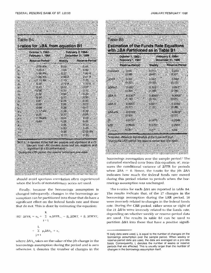
should avoid spur ous con-relation often expen-iencedwhen the levels of nionstation~u’vsenies an-c used.

Finally, because the Iinin-r-owings assumption ischanged infr-equentls’, changes in the borrowings as-sumption can lie partitioned into those that do have asignificant effect on the federal funds n-ate and thosethat dlo not. This is clone by estimating the equation:

KB2~Atl’R, — a,, -~- > cv4FFR,, + (3,, ~f)R’I’, + ft ~MiRNT,

n-

iS” I

+ ~ p~ABA,,,+ 8,.

j—t

syliei-e ABA,~takes on the value of the jth change in thebon-n-owings assumption dur-ing the pen-iod and is zerootherwise. I.. denotes the number rif changes in the

/ ‘1, / ‘ k,ç / ,,

1 i/t A —

/ / \/\ /

Estin*tI*noS*cs~dsRate ~qE~ttons~*~tfr4$*$rt1t1one*,~fltt*$iBi

A’ iJ1’~J~ Foetotr~eni~ot~ Febn~sfl~>914-~ebnrsry’t19$ beSSsiS is>

borr-ownngs assumption over the sample pei-iod.’ Theestimated standar-d error ft-tim this equation, o’~,mea—sun-es the conditional van’iance of AFFR fcir periodswhen ABA = 0. Hence, the t-ratio for the jth ABAindicates how much the federal frindls n-ate movedduring this period relative to per-iods when the lion-—r-owings assumption was unchanged.

The t—ratios for each ABA an’e n-epor-ted in table B4.The r-esults indicate that, of the 17 changes in the

bon-r’owings assumption during the 1.88 per’iod, 10wer-e inversely related to changes in the federal fundsn’ate. IJun-ing the CR8 period, either seven ot eight ofthe 21 ABAs wer-e niver-sely n-elated to the funds n-ate,depending on whether weekly or reserve-period dataare used. The results in table B4 can be used topantition ABA into those that have a positive signifi-

‘If daily data were used, L is equal to the number of changes on theborrowings assumption over the sample period. When weekly orreserve-period data are used, the data are averaged on a pro-ratabasis, Consequently, L denotes the number of weeks or reserveperiods that are affected. This is usually larger than the number ofchanges in the borrowings assumption itself,

FEDERAL RESERVE BANK OF ST. LOUIS JANUARY/FEBRUARY lOSS

cant effect on the funds nate, ABA-A, those that have asignificant negative effect, ABA-AN, and alt other’s,ABA-B. This was done by including in the A on’ ANgn-oups all ABAs that are significant at the 025 pci-cent

level using standard analysis. Those changes in BAthat are in the A (ir AN groups ar-c designated con-n-c-

spondingly in table B4.

Estimates of the samne basic equation with the parti-tioned data at-c presented in table B5. In all cases,

except the single observation in the A group dluringthe LRR period, the coefficients on the A anti ANpartitions an-c significant at the 5 pen-cent level - Mnin’eimportantly, the coefficients on the changes in tImliorrowings assuriiption in the B partition. which ac-count for the vast majority of changes in the fior-r’ow—ings assumption, were uniformly insignificant at the 5percenit level. This evidence indicates that the linkbetween changes in the bon’n-owings assumption andthe fediem-al funds rate is, at best, weak.