The 1 N expansions - Eduardo Fradkin (Physics)

17

The 1/N expansions

As we saw in chapter 16, perturbation theory, even when applicable, onlydescribes a regime of the theory. In the case of the non-linear sigma modelin D = 2 dimensions, and in Yang-Mills theory in D = 4 dimensions, therunning coupling constant is weak only at short distances but the long-distance behavior is inaccessible to perturbation theory since the couplingconstant runs to large values, outside the perturbative regime. So we havetheories that at low energies have a vacuum state that is essentially differentthan the free field ground state. To understand the physics of the actualground state requires the use of non-perturbative methods. A key tool inthis respect is the study of the generalizations of the theories of interest intheir “large-N” limits. Here N can mean the rank of the symmetry groupor the rank of the representation. The behavior is different in each case.We begin by considering first the simpler, and more tractable, case of scalarfields.

There is a long history of studying theories in this limit, both in StatisticalPhysics and in Quantum Field Theory. In Statistical Physics it goes back tothe classic work by Berlin and Kac on what they called a “spherical model”of a phase transition (Berlin and Kac, 1952). This solvable model was lateron shown to be equivalent to the large-N limit of the classical Heisenbergmodel (with an N -component order parameter) by Stanley (Stanley, 1968).With the advent of the renormalization group, this limit was studied byS.-K. Ma in the context of a φ4 theory with a global O(N) symmetry (Ma,1973). In Quantum Field Theory, large-N limits became a mainstay toolto study non-perturbative the behavior of asymptotically free theories suchas non-linear sigma models (Brezin and Zinn-Justin, 1976b), the CP

N−1

models, the Gross-Neveu models (Gross and Neveu, 1974) and, particularly,Yang-Mills gauge theory (’t Hooft, 1974; Witten, 1979b). These methodshave also been extensively used in theories of the Kondo problem (Read

590 The 1/N expansions

and Newns, 1983), quantum antiferromagnetism (Sachdev and Read, 1991),and in the study of quantum phase transitions (Sachdev, 1999). It has alsoplayed an important role in the theory of random matrices (Mehta, 2004).

17.1 The φ4scalar field theory with O(N) global symmetry

Let us begin by considering the O(N) φ4 theory. This theory has a scalarfield φ(x) which is an N -component vector that transforms in the funda-mental (vector) representation of the global symmetry group O(N). The(Euclidean) Lagrangian is

L =12(∂µφ(x))2 + m

20

2φ2(x) + g

4!N(φ2(x))2 (17.1)

where, as usual, repeated indices are summed over. Notice that we havemade the replacement of the conventional coupling constant λ ↦

g

N. Shortly

we will see the necessity of this replacement. The interaction vertex of theO(N) theory is shown in Fig.17.1, where, for clarity, we have formally splitthe contact interaction.

a

a

b

b

g

N

Figure 17.1 The interaction vertex of O(N) scalar field theory with cou-pling constant λ =

g

N.

17.1.1 Diagrammatic approach to the large-N limit

We will now ask what is the dependence on N of the Feynman diagrams ofthe 1PI two-point function, i.e. the φ field self-energy. The diagrams up toone-loop order are shown in Fig.17.2. It is easy to see that since each one-loop diagram contributes with a factor of the coupling constant, the rainbowdiagram of Fig.17.2a contributes with a factor of g

N, while the tadpole di-

agram of Fig.17.2b contributes with a factor of g

NN = g, where the factor

of N comes from the independent sum over the index b running inside theloop. Thus, in the limit N → ∞, the leading term is Fig.17.2b and Fig.17.2ais a 1/N correction.

To see the emerging pattern in the large N limit, we will look at the

17.1 The φ4 scalar field theory with O(N) global symmetry 591

a a

a

(a)

a a

b

(b)

Figure 17.2 One-loop contributions to the 1PI two-point function of theφ field in the O(N) theory; a) the rainbow diagram and b) the tadpolediagram.

two-loop diagrams of Fig.17.3. By counting powers of N , we see that the

a a

b c

(a)

a a

b

(b)

a a

a

b

(c)

Figure 17.3 two-loop contributions to the 1PI two-point function of the φfield in the O(N) theory; a) the two-loop tadpole diagram, b) the rainbow-tadpole two-loop diagram, and c) the two-loop rainbow diagram.

diagram of Fig.17.3a contributes with a factor of g2

N2N2= g

2, that the dia-

gram of Fig.17.3b contributes with a factor of g2

N2N =g2

N, and the diagram

of Fig.17.3c contributes with a factor of g2

N2 . Hence, only the diagram ofFig.17.3a survives in the N → ∞ limit.

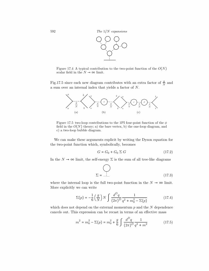
We now see the pattern: diagrams in which the number of independentsums over the internal indices is equal to the order in perturbation theoryhave a finite limit as N → ∞, whereas the contributions of the other dia-grams can be organized as a formal expansion in powers in 1/N . A typicaldiagram that contributes to the two-point function in the N → ∞ limit isshown in Fig.17.4. In fact, we have already reached this conclusion alreadyin Section 11.6 where we showed that this sum of diagrams (also knownas the Hartree approximation) yields the self-consistent expression for theone-loop self-energy of Eq.(11.60).

Moving on to the four-point function, it is easy to see that as N → ∞

the only surviving contributions is the sum of the bubble diagrams shown in


Figure 17.4 A typical contribution to the two-point function of the O(N)scalar field in the N → ∞ limit.

Fig.17.5 since each new diagram contributes with an extra factor of g

Nand

a sum over an internal index that yields a factor of N .

a

a

b

b

g

N

(a)

a

a

b

b

g

N

g

N

c

(b)

a

a

b

b

g

N

g

N

c dg

N

(c)

Figure 17.5 two-loop contributions to the 1PI four-point function of the φfield in the O(N) theory; a) the bare vertex, b) the one-loop diagram, andc) a two-loop bubble diagram.

We can make these arguments explicit by writing the Dyson equation forthe two-point function which, symbolically, becomes

G = G0 +G0 Σ G (17.2)

In the N → ∞ limit, the self-energy Σ is the sum of all tree-like diagrams

Σ = (17.3)

where the internal loop is the full two-point function in the N → ∞ limit.More explicitly we can write

Σ(p) = −16( g

N)N ∫ d

Dq(2π)D 1

q2 +m20 − Σ(p) (17.4)

which does not depend on the external momentum p and the N dependencecancels out. This expression can be recast in terms of an effective mass

m2= m

20 −Σ(p) = m

20 +

g

6∫ d

Dq(2π)D 1

q2 +m2 (17.5)

17.1 The φ4 scalar field theory with O(N) global symmetry 593

We recognize that this is just the renormalized mass (squared) at one-looplevel, c.f. Eq.(11.62), discussed in Chapter 11. The only difference is that inthe N → ∞ limit this expression is exact. Thus, in this theory, the large N

limit is equivalent to a self-consistent one-loop approximation.

We now have to consider the 1PI four-point vertex function Γ(4)ijkl(p1, . . . , p4),

which by symmetry can be written is

Γ(4)ijkl(p1, . . . , p4) ==

13N

[δijδklF4(p1 + p2) + δikδjlF4(P1 + p3) + δilδjkF4(p1 + p4)] (17.6)

The quantity F4(p) in the large-N limit is the sum of the bubble diagrams

≡ + + +. . .

(17.7)More explicitly, we can write the exact expression (in the N → ∞ limit) forthe sum of bubble diagrams F4(p)

F4(p) = g

1 + g

6I(p) (17.8)

where I(p) is the one-loop bubble diagram

I(p) = ∫ dDq(2π)D 1(q2 +m2)((p− q)2 +m2) (17.9)

Therefore, the sum of bubble diagrams yields the form of the effective inter-action in the large-N limit. The sum of bubble diagrams is reminiscent of theRandom Phase Approximation of Bohm and Pines (Pines and Bohm, 1952;Pines and Nozieres, 1966) widely used in the theory of screening in electronfluids. In this context, the sum of tadpole diagrams leading to Eq.(17.3) isanalogous to the Hartree approximation of the electron self-energy in thetheory of the electron fluids.

The expression for I(p) is UV finite for D < 4 and has a logarithmicdivergence as D → 4−. The methods that we introduced to compute theseintegrals yield the result (in D Euclidean dimensions)

I(p) = Γ (2− D

2)

(4π)D/2 24−D ∫ 1

0du((1− u

2)p2 + 4m2)(D−4)/2

(17.10)

The important observation here is that if the renormalized mass vanishes, theIR behavior of the bubble leads to an IR singularity of the four point functionΓ(4)(p) ∝ p

4−D. As we will see below, this result means that the effective


coupling constant must have a non-trivial scale dependence, as dictated bythe RG flow.

17.1.2 Path-integral approach

The diagrammatic analysis of the large-N limit of φ4 theory is useful but ithas the drawback that it seemingly applies only to the symmetric phase ofthe theory in which the O(N) symmetry is not spontaneously broken. Al-though a similar diagrammatic analysis can be done in the broken symmetryphase, there is a more general approach that uses the large-N limit of thepath integral for the partition function. To this end we introduce an auxil-iary (Hubbard-Stratonovich) field α(x) to rewrite the partition function forthe theory with the Lagrangian of Eq.(17.1)

Z =∫ Dφ exp(−∫ dDx [1

2(∂µφ)2 + m

20

2φ2+

g

2N(φ2)2])

=∫ Dα∫ Dφ exp (−∫ dDx [1

2(∂µφ)2 + m

20

2φ2−

N

2gα2+ αφ

2])=∫ Dα (Det [−∂2 +m

20 + α])−N/2

exp (+∫ dDxN

2gα2) (17.11)

After integrating-out the φ fields, we can rewrite the partition function asa path-integral over the field α(x),

Z = ∫ Dα exp (−NSeff[α]) (17.12)

where the effective action Seff[α] is

Seff[α] = 12tr ln [−∂2 +m

20 + 2α] − 1

2g∫ d

Dx α

2(x) (17.13)

Therefore, the large-N limit of φ4 theory is the semiclassical limit of thetheory of the field α, whose effective action is given by Eq.(17.13). Hence, inthe N → ∞ limit the path integral for the partition function is determinedby the configurations αc(x) that make the effective action stationary, i.e.the classical field αc(x) that satisfies the saddle-point equation

δSeff

δα= 0 (17.14)

which implies that the gap equation

G(x, x;m2) = αc

g (17.15)

17.2 The large-N limit of the O(N) non-linear sigma model 595

must be satisfied. Here we have set m2= m

20 + 2αc and

G(x, y;m2) = ⟨x∣ 1

−∂2 +m2 ∣y⟩ (17.16)

is the propagator of a massive scalar field of mass squared m2. Hence, the

classical field αc obeys the equation

αc

g = ∫ dDp(2π)D 1

p2 +m20 + 2αc

(17.17)

By analogy with the BCS theory of superconductivity, equations of thistype are generally called “gap equations”. It should be apparent that theself-energy we computed using the Dyson equation and the classical field arerelated by Σ = −2αc.

Returning to the effective action of the field α(x), we see that the 1PItwo-point function of the field α(x) = α(x) − αc is

Γ(2)αα(x, y) = 2G(x, y;m2)G(y, x;m2) + 1

g δ(x − y) (17.18)

which, in momentum space, is easily seen to be the inverse of F4(p)/g. Werecognize the first term of the right hand side of this equation as the bubblediagram.

This analysis require a renormalization prescription. It should also besupplemented by an analysis of the broken symmetry state. For brevity wewill do that only in the next section devoted to the large-N limit of thenon-linear sigma-model.

17.2 The large-N limit of the O(N) non-linear sigma model

We will now turn to the case of the O(N) non-linear sigma model andits large-N limit. We have already discussed that, in the Euclidean metric,the non-linear sigma model is the formal continuum limit of the classicalHeisenberg model. It has been know since the 1960s (Stanley, 1968) that thelarge-N limit of this model ie equivalent to the “spherical model” proposedin 1952 by Berlin and Kac (Berlin and Kac, 1952). Here we will work in D

Euclidean dimensions.As discussed in earlier chapters, at the classical level the O(N) non-linear

sigma model can be regarded as a limit of a φ4 theory in its broken symmetrystate. Indeed, we can rewrite the Euclidean Lagrangian of and N -componentφ4 theory as

L =12(∂µφ)2 + λ

4!(φ2

− φ20)2 (17.19)


which, in the λ → ∞ limit, becomes the Lagrangian of a non-linear sigmamodel with and N component unit-vector field n(x) = (σ(x),π(x)), suchthat n = σ

2+π

2= 1 as a constraint everywhere in D-dimensional Euclidean

space-time. The partition function of the O(N) non-linear sigma model isthe path integral

Z[H,J] = ∫ DσDπ δ(σ2 + π2− 1) exp (−S

g ) (17.20)

where 1/g = φ20. Here, the δ-function acts at all points of D-dimensional

Euclidean space-time. The action S is

S = ∫ dDx [1

2(∂µσ)2 + 1

2(∂µπ)2 −Hσ − J ⋅ π] (17.21)

where (H,J) is a symmetry-breaking field. We will now see that even thoughclassically (and in perturbation theory for D > 2) this is a theory of a brokensymmetry state, this theory has (again for D > 2) both a broken symmetryphase and a symmetric phase separated by a critical (and non universal)value of the dimensionful coupling constant g.

17.2.1 Large-N limit

That the non-linear sigma model has a finite large-N limit can be gleanedfrom the perturbative expression for the 1PI two-point function of the π

field, presented last chapter in Eq.(16.158) and in Fig.16.3. There we seethat as N becomes large, we can have a finite limit provided the couplingconstant g and the field H must be scaled by N and the field π must alsobe scaled by an appropriate power of N .

Here we will use a functional approach to study the large-N limit. Webegin by implementing the constraint by means of an integral representationof the δ-function in terms of a Lagrange multiplier field α(x), in terms ofwhich the partition function now reads

Z = ∫ DσDπDα exp (−Sg + ∫ d

Dxα(x)2g

(1 − σ2(x) − π

2(x))) (17.22)

Let us rescale the N − 1-component fields π =√gϕ which in turn can be


integrated-out to yield

Z = ∫ DσDα (Det[−∂2 + α])−(N−1)/2

× exp (12∫ d

Dx∫ d

Dy G(x − y;α) J(x) ⋅ J(y))

× exp (−1g ∫ d

Dx12(∂µσ)2 −Hσ −

12α(σ2 − 1)) (17.23)

where the kernel G(x − y;α) satisfies

(−∂2 + α(x))G(x − y;α(x)) = δ(x − y) (17.24)

for an arbitrary configuration of the Lagrange multiplier field. Hereafter wewill drop the explicit x-dependence of the field α. For the time being, wewill set the sources J(x) = 0 (although later they will be restored).

It will be convenient to rescale the bare coupling constant g and the fieldσ as follows

g =g0

N − 1, σ(x) = √

g(N − 1)m(x) (17.25)

The effective action of the rescaled field m(x) and of the Lagrange multiplierfield α becomes

Seff(m,α,H) = ∫ dDx [1

2(∂µm)2 + 1

2αm

2−

α

2g0−

Hm√g0

]+ 12tr ln (−∂2 + α)

(17.26)and the partition function is

Z[H] = ∫ DmDα exp (−(N − 1)Seff(m,α,H)) (17.27)

Hence, once again, the large-N limit is the semiclassical limit, in this case ofthe effective action for the fieldsm and α coupled to the sourceH. Therefore,in the large-N limit, the partition function of Eq.(17.27) is dominated bythe configurations that leave the effective action of Eq.(17.26) stationary.By varying Seff with respect to the field m(x) we get

δSeff

δm(x) = −∂2m(x)+ α(x)m(x) − H√

g0= 0 (17.28)

Likewise, by varying Seff with respect to α(x) we obtain

δSeff

δα(x) = −12g0

+12m

2(x) + 12

δ

δα(x) tr ln (−∂2 + α) = 0 (17.29)

whereδ

δα(x) tr ln (−∂2 + α) = ⟨x∣ 1

−∂2 + α∣x⟩ (17.30)


Hence, we obtain a second saddle point equation

⟨x∣ 1

−∂2 + α∣x⟩ +m

2(x) − 1g0

= 0 (17.31)

We will now seek a uniform solution of Eqs. (17.28) and (17.31) of the form

σ(x) = M, α(x) = α (17.32)

with H constant, and M2= g0m

2. Thus, the solution of Eq.(17.28) is

α =H

M(17.33)

while Eq.(17.31) becomes

g0⟨x∣ 1

−∂2 + HM

∣x⟩ = 1−M2

(17.34)

or, what is the same

g0 ∫ dDp(2π)D 1

p2 + HM

= 1−M2

(17.35)

17.2.2 Renormalization

Provided H/M ≠ 0, Eq.(17.35) is IR finite. However, for D ≥ 2 the integralis UV divergent. We will absorb the strong dependence in the UV in a setof renormalization constants. Thus, we define a dimensionless renormalizedcoupling constant t, a renormalized MR and a renormalized HR through therelations (here κ is an arbitrary momentum scale) (see Eqs. (16.161) and(16.162))

g0 =tκ−ϵZ1

M =Z1/2

MR

H =Z1Z−1/2

HR (17.36)

where we have set ϵ = D − 2, and Z is the wave function renormalization.Notice that

H

M=

Z1

Z

HR

MR(17.37)

With these definitions Eq.(17.35) becomes

tκ−ϵZ1

Z∫ d

Dp(2π)D 1

p2 + HR

MR

Z1

Z

=1Z

−M2R (17.38)


We have encountered the integral in this equation several times before. It isgiven by

∫ dDp(2π)D 1

p2 + µ2=

1(4π)D/2Γ (− ϵ2)µϵ (17.39)

Using this result we can recast Eq.(17.38) as

tκ−ϵ (Z1

Z)1+ϵ/2 (HR

MR)ϵ/2 1(4π)D/2Γ (− ϵ

2) =

1Z

−M2R (17.40)

We now use dimensional regularization with (quasi) minimal subtractionby defining Z and Z1 in such a way that the singular dependence in ϵ iscancelled. Thus, we choose

Z = Z1 (17.41)

and1Z

= 1 + t1(4π)D/2Γ (− ϵ

2) (17.42)

With these choices Eq.(17.40) become

1 −M2R =

ttc

(1 − ( HR

κ2MR

)ϵ/2) (17.43)

which is finite as ϵ → 0. Here we introduced the quantity tc,

tc = (D − 22

) (4π)D/2Γ (2 − D

2) (17.44)

which we will shortly identify with the value of the critical coupling con-stant. This equation relates MR, the (renormalized) expectation value ofthe sigma field, to the renormalized dimensionless coupling constant t andthe renormalized symmetry breaking field HR. In the statistical mechanicalinterpretation, this is the equation of state (in the N → ∞ limit).

17.2.3 Phase diagram and spectrum

We will now show that, in the N → ∞ limit and for D > 2, the non-linearsigma model has a phase transition between a broken symmetry phase and asymmetric phase. To this end, let us seek a solution to Eq.(17.43) for HR = 0and MR ≠ 0, i.e.

1−M2R =

t

2πϵ(17.45)


and notice that, as MR → 0, t approaches (from below) the value tc given inEq.(17.44) which defines the critical coupling constant. It is worth to notethat, as expected, tc → 0 as ϵ→ 0. Using this expression for tc, we can writeEq.(17.45) as

1 −M2R =

ttc

(17.46)

or, what is equivalent,

MR = (1 − ttc)β (17.47)

where the exponent is β = 1/2. We already found this result in our studyof the perturbative renormalization group where we noted that β → 1/2as n → ∞. Hence, we expect that there will be corrections to this resultif we go beyond the N → ∞ limit. Thus, we see that for t < tc the O(N)symmetry is indeed spontaneously broken.

Let us now examine the behavior for t > tc. We will now use the definitionof tc of Eq.(17.44), to write Eq.(17.45) in the simpler form

1−M2R =

ttc

(1− ( HR

MRκ2)ϵ/2) (17.48)

We now recall that, by dimensional analysis and the Ward identity, thesusceptibility χR is

χR = κ2MR

HR(17.49)

in terms of which we can write

1−M2R =

ttc

(1 − [χR(t,HR)]−ϵ/2) (17.50)

We now take the limit HR → 0 and MR → 0 holding χR fixed, and obtain

χR = (1− ttc)−γ (17.51)

where the exponent is γ =2ϵ(again in the N → ∞ limit).

Having understood the question of spontaneous symmetry breaking, wewill now inquire the behavior of the π fields. We expect that the π fieldsshould be the Goldstone bosons of the broken symmetry state and, hence,should be massless in the broken symmetry phase, and massive in the unbro-ken phase. Moreover, we also expect the σ field to be massive in the brokenphase and that all the masses become equal as H → 0.

To this end we now restore the fields J ≠ 0, the sources of the π fields.


Although, in principle, we obtain more complicated saddle point equationsif J ≠ 0, in practice we can still use our solutions obtained for J = 0 in theregime in which J is infinitesimally small (i.e. “linear response”). Hence,we can approximate the kernel G(x, y;α) that enters in Eq.(17.23), by itsapproximate form with α = α =

HM

=HR

MR. We readily see that, in this limit,

the two-point function of the π fields is

⟨π(x) ⋅ π(y)⟩ = G (x, y; HR

MR) (17.52)

In other words, provided HR

MR≠ 0, the π fields are massive and their mass

(squared) is

m2π =

1

ξ2π=

HR

MR(17.53)

where ξπ is the correlation length of the π fields, which, as we see, is givenby

ξπ = (χRκ−2)1/2 = κ−1 88888881 −

tct

8888888−ν

(17.54)

where ν = γ/2 = 1/ϵ (again, as N → ∞).Thus, in the symmetric phase, we find that at HR → 0,

m2π = χ

−1R = m

2σ (17.55)

where m2σ is the mass (squared) of the σ field. Hence, for t > tc we have a

spectrum of N massive bosons forming a multiplet of O(N) (as we should!).On the other hand, for t < tc, the symmetry is spontaneously broken andMR ≠ 0 as HR → 0. Hence, in the broken symmetry state m

2π = 0 and we

have (as we should!) a spectrum of N − 1 massless (Goldstone) bosons.In the special case of D = 2, the correlation length ξπ = ξσ = ξ, becomes

ξ = m−1

= κ−1

exp (2πt) (17.56)

This result shows the dependence of the correlation length on the dimen-sionless coupling constant t is an essential singularity. This implies that theN → ∞ is truly non-perturbative. We will encounter this behavior in allasymptotically free theories.

17.2.4 Renormalization group

We now return to the definitions of Eq.(17.36) to obtain the renormalizationgroup functions in the large-N limit. We begin with the beta function for


the dimensionless coupling constant t,

β(t) = κ ∂t∂κ

888888B (17.57)

were we hold the bare theory fixed. From the definition g0 = tκ−ϵZ1 we find

β(t) (1 + t∂ lnZ1

∂t) = ϵt (17.58)

Using the expression for Z1 (and of Z) of Eq.(17.42), and the definition oftc of Eq.(17.44), we find that the beta function is exactly given by

β(t) = ϵt − ϵt2

tc(17.59)

Hence, in the N → ∞ limit the beta function terminates at the quadraticorder in t, where it agrees with the one-loop result, c.f. Eq.(16.177), in thelarge-N limit and for D = 2 + ϵ. We see that, for D > 2, the beta functionhas two zeros (or fixed points): a) a trivial fixed point at t = 0, and b) anon-trivial fixed point at t = tc. Furthermore, the slope of the beta functionis negative at the non-trivial fixed point. Hence, this fixed point us unstablein the IR (and hence stable in the UV). Conversely, the trivial fixed pointis stable in the IR and unstable in the UV.

On the other hand, for D = 2 the beta function simply becomes

β(t) = κ ∂t∂κ

= −t2

2π(17.60)

which says that the O(N) non-linear sigma model is asymptotically freein D = 2, and the trivial fixed point at t = 0 is IR unstable. As we saw,the N → ∞ limit predicts that the theory is in a massive phase with anunbroken global symmetry for all values of the coupling constant.

Similarly, we can compute the renormalization group function γ(t),γ(t) = β(t)∂ lnZ

∂t(17.61)

and find

γ(t) = ttcϵ (17.62)

Hence, the anomalous dimension η at the non-trivial fixed point at tc is

η = γ(tc) − ϵ = 0 (17.63)

In other terms, the anomalous dimension η = O(1/N), and to determineit requires a computation of the leading correction in the 1/N expansion.

17.3 The CPN−1 model 603

This is consistent with the result we obtained in the 2 + ϵ expansion, c.f.Eq.(16.197), where we found that η ∝ 1/N .

An important moral of this discussion is that, while for D > 2 the per-turbative definition of the theory, based on an expansion in powers of thecoupling constant, is non-renormalizable, here we find that the theory de-fined around the non-trivial fixed point is renormalizable. Notice that wewere able to access this UV fixed point only by means of the use of thelarge-N limit. In principle, the 2 + ϵ expansion could be used to the sameend . However, this presents technical difficulties associated with the behav-ior of the expansion that we will not discuss here.

17.3 The CPN−1

model

We will now turn to the CPN−1 model (D’Adda et al., 1978; Witten, 1979b;Coleman, 1985), introduced in section 16.5.1. As we showed there, thesemodels can be described by an N -component complex field z(x) of unitnorm, i.e. z(x) = (z1(x), . . . , zN (x)) with zi(x) ∈ C and z

†(x) ⋅ z(x) =

∑Ni=1 ∣zi(x)∣2 = 1, minimally coupled to a U(1) gauge field Aµ(x). The

action of this model is (c.f. Eq.(16.103))

S[zα, z∗α ,Aµ] = 1g ∫ d

Dx ∣(∂µ − iAµ(x))z(x)∣2 , (17.64)

Here g is the coupling constant, which has units of [L]D−2, as in the case ofthe O(N) model. As we saw, this model is invariant under the local U(1)gauge transformations,

z(x) ↦ exp(iφ(x))z(x), Aµ(x) ↦ Aµ(x) + ∂µφ(x) (17.65)

Notice that the gauge field only enters in the action through the covariantderivative, and that we do not have a separate term for the gauge field, aswe would in quantum electrodynamics.

In the absence of the U(1) gauge field, this would be a theory of anN -component complex field with unit norm or, what is equivalent, a 2N -component real vector of unit length. This would be a non-linear sigmamodel with SU(N) global symmetry or, equivalently O(2N). Hence, forD > 2, we would expect to have a broken symmetry state with 2N − 1Goldstone bosons. However, in the CPN−1 model a U(1) subgroup of SU(N)has been gauged. In this situation, we expect that in the broken symmetrystate there is a Higgs mechanism (see section 18.11) and, consequently, oneof the otherwise 2N−1 massless Goldstone bosons should be absent, “eaten”by the gauge field which should be massive in this phase. On the other hand,


in the symmetric phase, the z fields should be massive, and the gauge fieldshould be strongly fluctuating.

Here we will use a functional approach very similar to what we did inthe case of the O(N) non-linear sigma model. Thus, we implement the localconstraint, z†

z = 1 with an integral representation of the delta functionusing a (real) Lagrange multiplier field α(x). The partition function of theCP

N−1 model is

Z = ∫ DzDz†DAµDα exp (−1

g ∫ dDx [∣(∂µ − iAµ)z∣2 − α(z†

z − 1)])(17.66)

In order to have a well defined large-N limit we will rescale the couplingconstant as g = g0/N .

We can now integrate-out the N -component complex field z and obtain,after rescaling the z fields by

√g0, the partition function in terms of the

effective action for the gauge field Aµ and the Lagrange multiplier field α,

Seff[Aµ,α] = tr ln (−Dµ[Aµ]2 + α) − 1g0

∫ dDxα(x) (17.67)

where Dµ[A] = ∂µ − iAµ is the covariant derivative. The partition functionnow has the form

Z = ∫ DAµDα exp (−NSeff[Aµ,α]) (17.68)

Notice that, unlike what we did in the O(N) non-linear sigma model, weare treating symmetrically all the components of the z field. Although wewill find a phase transition, the analysis of the broken symmetry state willbe easier in a somewhat less symmetric formulation.

Clearly, as N → ∞ this partition function will be dominated by the clas-sical configurations that leave the effective action stationary. The differencebetween the O(N) non-linear sigma model and the CP

N−1 model is that,in addition to the Lagrange multiplier field α, we now have the gauge fieldAµ. Thus we will have two saddle point equations, each requiring that theeffective action be stationary under separate variations of the gauge fieldand of the Lagrange multiplier field.

Thus we find two conditions. The first one, obtained by varying Seff withrespect the Lagrange multiplier field α(x),

δSeff

δα(x) = 0 (17.69)


implies that

1g0

= ⟨x∣ 1

−D[Aµ]2 + α∣x⟩ (17.70)

The second saddle point equation, obtained by varying with respect to thegauge field Aµ(x),

δSeff

δAµ(x) = 0 (17.71)

is the condition that, at the classical level, the U(1) gauge current vanishes,δS

δAµ(x) = jµ[A] = 0 (17.72)

where S is the action of the CPN−1 model. Thus, in the absence of external

sources, we can set the classical configuration of the gauge field ⟨Aµ⟩ = 0,which trivially satisfies the condition of a vanishing U(1) gauge current.

Thus, the only equation to be solved in the large-N limit, Eq.(17.70), isthe gap equation

1g0

= ⟨x∣ 1

−∂2 + α∣x⟩ = ∫ d

Dp(2π)D 1

p2 + αc

(17.73)

Notice that the classical value of the Lagrange multiplier, αc, plays the roleof a mass term for the z fields, and

G(x − y∣αc) = ⟨x∣ 1

−∂2 + αc

∣y⟩ (17.74)

is the propagator for the z field.We have encountered the integral on the right hand side of Eq.(17.73)

several times, most recently in Eq.(17.39). This integral is UV divergent forD > 2 and logarithmically divergent for D = 2. Thus, as before, we needto define renormalized quantities. Here it will suffice to renormalize thecoupling constant g

20 . Using dimensional analysis we define a renormalized

dimensionless coupling constant t,

g0 = tκ−ϵZ (17.75)

where Z is a renormalization constant and κ is the renormalization scale.Using the expression of Eq.(17.39) for the integral, the saddle-point equationof Eq.(17.73) becomes

1Z

= tκ−ϵ 1(4π)D/2Γ (− ϵ

2)αϵ/2c (17.76)


Once again, we will use the minimal subtraction procedure to cancel thesingular dependence of ϵ. To this end we choose Z to have the same form asin the non-linear sigma model, Eq.(17.42). This choice results in the saddle-point equation to become

1 =ttc

(1 − (αcκ−2)ϵ/2) (17.77)

where tc is the same value for the critical coupling that we found for thenon-linear sigma model, c.f. Eq.(17.44). We can now readily solve for thevalue αc and find

αc = κ2 (1 − tc

t)2/ϵ (17.78)

This solution is only allowed if t > tc. For t < tc, the only possible solutionis αc = 0.

In other words, for D > 2 and in the limit N → ∞, the CPN−1 model

has two phases separated by a phase transition at tc. For t < tc the z fieldsare massless, and for t > tc they are massive with mass m

2z = αc. On the

other hand in D = 2, tc → 0 and there is only one phase and the z fieldsare massive for all values of the coupling constant. It is easy to see that, inD = 2, the mass (squared) is

m2z = αc = κ

2exp (−π

t) (17.79)

In other words, in D = 2 the CPN−1 model is be asymptotically free and

exhibits dynamical mass generation.

That the CPN−1 model is asymptotically free in D = 2 can be seen by

computing the beta function (in the large-N limit)

β(t) = κ∂t

∂κ

888888B = ϵt −ϵtct2

(17.80)

which is the same as the O(N) non-linear sigma model in the N → ∞ limit.Thus, here too, for D > 2 we have a UV fixed point at tc and a IR fixedpoint at t = 0. In D = 2 dimensions this theory is asymptotically free.

It is instructive to compute the leading corrections in the 1/N expansion.


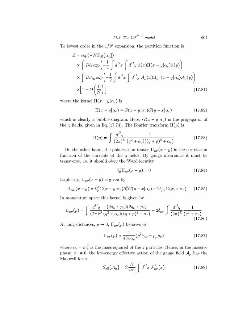
To lowest order in the 1/N expansion, the partition function is

Z = exp(−NSeff[αc])×∫ Dα exp (−1

2∫ d

Dx∫ d

Dy α(x)Π(x − y∣αc)α(y))

×∫ DAµ exp (−12∫ d

Dx∫ d

Dy Aµ(x)Πµν(x − y∣αc)Aν(y))

×[1 +O ( 1N

) ] (17.81)

where the kernel Π(x − y∣αc) is

Π(x − y∣αc) = G(x − y∣αc)G(y − x∣αc) (17.82)

which is clearly a bubble diagram. Here, G(x − y∣αc) is the propagator ofthe z fields, given in Eq.(17.74). The Fourier transform Π(p) is

Π(p) = ∫ dDq(2π)D 1(q2 + αc)((q + p)2 + αc) (17.83)

On the other hand, the polarization tensor Πµν(x − y) is the correlationfunction of the currents of the z fields. By gauge invariance it must betransverse, i.e. it should obey the Ward identity

∂xµΠµν(x − y) = 0 (17.84)

Explicitly, Πµν(x − y) is given by

Πuν(x − y) = ∂xµG(x − y∣αc)∂xνG(y − x∣αc) − 2δµνG(x, x∣αc) (17.85)

In momentum space this kernel is given by

Πµν(p) = ∫ dDq(2π)D

(2qµ + pµ)(2qν + pν)(q2 + αc)((q + p)2 + αc) − 2δµν ∫ dDq(2π)D 1(q2 + αc)

(17.86)At long distances, p → 0, Πµν(p) behaves as

Πµν(p) ≃ 148παc

(p2δµν − pµpν) (17.87)

where αc = m2z is the mass squared of the z particles. Hence, in the massive

phase, αc ≠ 0, the low-energy effective action of the gauge field Aµ has theMaxwell form

Seff[Aµ] = CN

4αc∫ d

Dx F

2µν(x) (17.88)


where Fµν = ∂µAν − ∂νAµ is the field strength of this “emergent” gaugefield, and C =

148π

.The z fields couple minimally to the gauge field Aµ. Thus, we see that in

the symmetric phase (with t > tc) the z particles will experience a long-range“Coulomb” interaction, and should form gauge-invariant bound states of theform z

∗αzβ . This is particularly strong inD = 2 space-time dimensions. In two

dimensions, as in the case of the O(N) non-linear sigma model, the theoryis asymptotically free and the coupling constant flows to large values. Thetheory is in a phase dominated by non-perturbative effects. In the large-Nlimit we find that tc = 0 and the fields are massive.

However there is more than that. InD = 2 dimensions (i.e. 1+1 Minkowskispacetime) the Coulomb interaction is linear, i.e.∝ ∣x−y∣, where x and y arethe spatial coordinates of the z particles. This can be checked by computingthe expectation value of the Wilson loop operator, corresponding to theworldlines of a heavy particle-antiparticle pair, see section 9.7. As we knowthe Coulomb interaction in 1+1 dimensions becomes V (R) = σR. This is aconfining potential. Hence, not only these bound states are very tight butthere are no z particles in the spectrum. We will return to the problem ofconfinement in gauge theory in a later chapter.

To study the broken symmetry state, with t < tc, we need to modifyour approach somewhat. Let us call the component z1 = z∥ and the N − 1remaining (complex) components z⊥. The Lagrangian now is

L =1g ∣Dµ[A]z∥∣2 + 1

g ∣Dµ[A]z⊥∣2 + αg (∣z∥∣2 + ∣z⊥∣2 − 1) (17.89)

In order to have a well defined large-N limit we now set g = g0(N − 1) (aswe did in the case of the non-linear sigma model). We can now integrate outthe N − 1 complex transverse fields, z⊥ and obtain the effective action

Seff[A,α, ρ] =(N − 1)tr ln (−D[A]2 + α) − N − 1g0

∫ dDx α(x)

+N − 1g0

∫ dDx[∣Dµ[A]z∥∣2 + α∣z∥∣2] (17.90)

This effective action is invariant under U(1) gauge transformations, andrequire that we fix the gauge. Here it is convenient to use the unitary gauge,z∥ = ρ ∈ R

+. The path integral for the field ρ (whose action is given insecond line of Eq.(17.90)) becomes

Z[A,α] = ∫ Dρ exp (−(N − 1)g0

∫ dDx [(∂µρ)2 + ρ2A2

µ + αρ2]) (17.91)

17.4 The Gross-Neveu model in the large N limit 609

The saddle point equation for α now is

1g0

−ρ2

g0= G(x, x∣α) (17.92)

and the saddle point equation for ρ is given by

−∂2ρ + ρA

2µ + αρ = 0 (17.93)

We will see solutions with A = 0 (as before). For g0 < gc0, i.e. t < tc, we will

set αc = 0 and seek a solution with ρ constant,

ρc = (1 − ttc)β (17.94)

with β = 1/2, in the N → ∞ limit.Thus, in the broken symmetry in D > 2, αc = 0 and the fields z⊥ are

massless, i.e. the 2(N − 1) Goldstone bosons. In this phase the gauge fieldAµ is massive, and the mass is ρ2c . So, in the broken symmetry phase thegauge field is “Higgsed”. In chapter 18 we will discuss the Higgs mechanism.In chapter 19 we will discuss the role of topology in field theory and returnto this model to discuss its instantons (and solitons) and their role.

17.4 The Gross-Neveu model in the large N limit

The Gross-Neveu model is a theory of interacting massless Dirac fermionsin 1 + 1 dimensions whose Lagrangian (in the Minkowski metric) is (Grossand Neveu, 1974)

L = ψai/∂ψa +g

2(ψaψa)2 (17.95)

Here the Dirac fermions are bispinors and the index a = 1, . . . , N labels thefermionic “flavors”. The theory has a global SU(N) flavor symmetry,

ψ ↦ Uψ (17.96)

where U ∈ SU(N). This theory is also invariant under a discrete chiraltransformations

ψ ↦ γ5ψ (17.97)

where γ5 is a hermitian 2×2 (with γ25 = I) Dirac matrix that anticommuteswith the Dirac matrices γµ. Hence, we have the algebra,

{γµ, γν} = 2gµνI, {γ5, γµ} = 0 (17.98)

with I being the 2 × 2 identity matrix and gµν = diag(1,−1) the metric ofD = 2-dimensional Minkowski space-time.


The Gross-Neveu model has a U(N) flavor symmetry and a Z2 chiralsymmetry. The fermion mass bilinear is odd under the discrete chiral trans-formation, Eq.(17.97), i.e.

ψψ ↦ −ψψ (17.99)

We will see that in the Gross-Neveu model the discrete chiral symmetry isbroken spontaneously and there is a dynamical generation of a mass for thefermions.

We can also define a chiral version of the Gross-Neveu model whose La-grangian is

L = ψai/∂ψa +g

2((ψaψa)2 − (ψaγ5ψa)2) (17.100)

which, in addition to the global SU(N) flavor symmetry, now has a U(1)chiral symmetry under the transformations

ψ ↦ eiθγ5 ψ (17.101)

The fermion bilinears can be put together into a two-component real vectorfield (ψψ, iψγ5ψ) that transforms as rotation by a global angle 2θ under theglobal U(1) chiral symmetry. We will see that this symmetry is (almost)spontaneously broken.

We will see that in D = 2 space-time dimensions the Gross-Neveu model(both chiral and non-chiral) are asymptotically free and exhibit dynamicalmass generation. As presented here, the non-chiral Gross-Neveu can also bedefined in higher dimensions with the proviso that it is no longer renormal-izable, meaning that with a suitable regularization it has a phase transition.In D = 4 dimensions this model is closely related to the Fermi theory ofweak interactions. The chiral version of the model is closely related to themassless Thirring model (in D = 2) and to the Nambu-Jona-Lasinio model(in D = 4) (Nambu and Jona-Lasinio, 1961).

17.4.1 The non-chiral Gross-Neveu model

Both versions of the Gross-Neveu model can be solved in the large-N limit.We begin with the non-chiral model, Eq.(17.95), by decoupling the four-fermion interaction term using a real scalar field σ. Upon scaling the couplingconstant g = g0/N , Lagrangian now is

L = ψai/∂ψa − σψaψa −N

2g0σ2

(17.102)

Now we see that the discrete chiral symmetry is equivalent to the Z2 (“Ising”)symmetry σ(x) ↦ −σ(x). Moreover, if the ⟨σ⟩ ≠ 0, the Ising symmetry


would to be broken spontaneously and ⟨ψψ⟩ ≠ 0 as well. Furthermore, anon-vanishing value for ⟨σ⟩ means that the fermions are became dynami-cally massive. Thus, this is a theory of dynamical mass generation by thespontaneous breaking of the chiral symmetry.

We now proceed to study this theory in the large-N limit. To this endwe first integrate out the fermionic fields and obtain the following effectiveaction for the σ field, Seff , with

Seff = −itr ln (i/∂ − σ) − ∫ dDxσ2

2g0(17.103)

where the first term now arises from the fermion determinant, i.e. fromsumming over fermion bubble diagrams. The partition function now is

Z = ∫ Dσ exp(iNSeff[σ]) (17.104)

Thus, as in the examples of the non-linear sigma model and the CPN−1

models, the large-N limit of the theory is the semiclassical approximationof a field that couples to a composite operator which in the case of theGross-Neveu model is the fermion mass bilinear, ψψ. The main differenceis that the Gross-Neveu model is a fermionic theory which is the reason forthe negative sign in front of the first term in the effective action, aside fromthe fact that the determinant involves the Dirac and not the Klein-Gordonoperator. Notice that we are working in Minkowski spacetime (hence thefactor of i in the first term of the effective action).

The stationary (saddle-point) equation is

∂Seff

∂σ(x) = −i⟨x∣ 1

i/∂ − σc∣x⟩ − σc

g0= 0 (17.105)

where σc is the saddle-point (uniform) value of the field σ(x), where we canidentify

Sab(x − y;m) = −i⟨x∣ 1

i/∂ −m∣y⟩δab (17.106)

with the Feynman propagator for a Dirac field with mass m ≡ σc.Using the momentum space form for the Dirac propagator we can readily

write the saddle-point equation as

tr∫ dDp(2π)D −i/p − σc

=σcg0

(17.107)

where the usual Feynman contour prescription has been assumed, and thetrace runs over the Dirac indices. This result, together with the definition of


the propagator, implies that at N = ∞ we can identify the chiral condensatewith

⟨ψψ⟩ = σcg0

(17.108)

Hence we have a chiral condensate if σc ≠ 0.We now use the Dirac algebra and a Wick rotation of the integration path

into the complex plane, ip0 ↦ pD, to write the saddle-point equation as

2∫ dDp(2π)D σc

p2 + σ2c=σcg0

(17.109)

Therefore, in this theory either σc = 0, and the chiral symmetry is unbroken,or we have a spontaneously broken discrete chiral symmetry state with σc ≠0. In this case the value of σc is the solution of the equation

2∫ dDp(2π)D 1

p2 + σ2c=

1g0

(17.110)

which is identical to the saddle point equation we found in the CPN−1 model,c.f. Eq.(17.73). Therefore it has the same solution.

Here too, we will first define a renormalized dimensionless coupling con-stant t, such that g0 = tκ

−ϵZ, where ϵ = D − 2. The resulting beta function

for the dimensionless coupling constant t has the same form as in the non-linear sigma model and the CP

N−1 model

β(t) = ϵt − ϵt2

tc(17.111)

but with a value of tc which is 1/2 of the value for the non-linear sigmamodel, Eq.(17.44).

We conclude that, for t > tc the fermion of the theory has the dynamicallygenerated mass

m = σc = κ (1− tct)1/ϵ (17.112)

and it remains massless for t < tc. Notice that, at N = ∞, the dynamicallygenerated mass m and the chiral condensate ⟨ψψ⟩ are related by

⟨ψψ⟩ = mg0

(17.113)

Here too, the case of D = 2 is special. Indeed, for D = 2 the theory isasymptotically free, and has a dynamically generated mass for all values ofthe coupling constant which, as N → ∞, is

m = σc = κ exp (−πt ) (17.114)


An alternative way to understand what happens is to compute the effectivepotential for a constant value of the field σ. AtN = ∞, the partition functionis just

Z[σc] = exp (−iNU(σc)) (17.115)

where σc is the constant value of the field σ that minimizes the potential

U(σc) = itr ln (i/∂ + σc) + ∫ d2xσ2c

2g0(17.116)

Using the properties of the 2D Dirac gamma matrices we have

tr ln(i/∂ − σc) = tr ln(∂2 + σ2c ) (17.117)

Then, after a Wick rotation, the potential becomes

U(σc) = tr ln(−'2+σ

2c ) + V

σ2c

2g0(17.118)

where V = L2 is the volume of D = 2 Euclidean spacetime. Hence, the

U(σ)

σ

Figure 17.6 Effective potential for the Gross-Neveu model.

problem reduces to the computation of the determinant of the EuclideanKlein-Gordon operator. Using the expression for the determinant of the 2DEuclidean Klein-Gordon operator computed using the ζ-function regulariza-tion in Section 8.8, see Eq.(8.212), we can write the potential U(σ) as

U(σ) = Vσ2

4π[ln (σ2

κ2) − 1] + V

σ2

2g0(17.119)

This potential, shown in Fig.17.6, has a minimum at the value of σc obtainedin Eq. (17.114).

The relation of Eq.(17.108) allows us to identify the fluctuations of the


field σ with the fluctuations of the chiral condensate. Thus, the propagatorof the σ field is the propagator of the composite operator ψψ. Expanding theeffective action to quadratic order in the fluctuations about its expectationvalue, σ(x) = σ(x) − σc, we find

Seff[σ] = −N

2∫ d

2x∫ d

2y σ(x)K(x− y)σ(y) (17.120)

where the kernel is

K(x − y) = tr (SF (x, y)SF (y, x)) + 1g0δ(x − y) (17.121)

Here SF (x, y) is the Feynman propagator for a massive Dirac field in twodimensions, which, upon a Wick rotation, falls off exponentially on distanceslong compared to ξ = σ−1c . This result also implies that the correlator of thefluctuations of the composite operator ∶ ψψ(x) ∶= ψψ(x) − ⟨ψψ(x)⟩, wherethe chiral condensate ⟨ψψ⟩ is given by Eq.(17.113), also falls off exponen-tially with distance,

⟨∶ ψψ(x) ∶∶ ψψ(y) ∶⟩ ∼ exp(−∣x − y∣/ξ) (17.122)

It is straightforward to see that, again in the N → ∞ limit, the compos-ite operator behaves as a scalar bound state with mass twice the fermionmass. Hence at N = ∞ the composite operator represents a bound state onthreshold, i.e. the binding energy is O(1/N).

17.4.2 The chiral Gross-Neveu model

We will close with a brief discussion of the chiral Gross-Neveu model whoseLagrangian is given in Eq.(17.100). This Lagrangian is invariant under theglobal U(1) chiral transformations of Eq.(17.101). This will lead to impor-tant changes. Since we know that in the non-chiral case the global discretechiral symmetry is spontaneously broken we may suspect that this may alsobe the case in the chiral Gross-neveu model as well. We will see that in2D spontaneous breaking of a U(1) symmetry is subtle and as a result thisclaim is almost (but not completely) correct.

To study this theory in its large-N limit (here N is the number of Diracfermion flavors) we will proceed as before and use a Hubbard-Stratonovichdecoupling of the quartic fermionic interactions. Since the Lagrangian hastwo quartic terms we will need two real scalar fields, which we will denoteby σ(x) and π(x), respectively. The partition function for D = 2 now is

Z = ∫ DψDψDσDπ exp (iS(ψ,ψ,σ,π)) (17.123)


where the action now is

S = ∫ d2xψ (i/∂ + σ(x) + iπ(x)γ5)ψ− N

2g0∫ d

2x (σ2(x) + π

2(x)) (17.124)

Under the continuous chiral symmetry of Eq.(17.101) the two componentreal field (σ,π) transforms as a rotation by a global angle 2θ.

Again, we now integrate out the fermions and obtain the effective actionfor the fields σ and π,

Seff[σ,π] = −iNtr ln (i/∂ + σ(x) + iπ(x)γ5) − N

2g0∫ d

2x (σ2(x) + π

2(x))(17.125)

The U(1) symmetry requires that the effective potential can only dependon σ2c + π

2c , where σc and πc are the solutions of the saddle point equations.

After tracing over the Dirac indices and a Wick rotation of the integrationcontours, the saddle point equations are

2σc ∫ d2p(2π)2 1

p2 + σ2c + π2c=σcg0

, 2πc ∫ d2p(2π)2 1

p2 + σ2c + π2c=πcg0

(17.126)

Therefore, if (σc,πc) is a solution of these saddle-point equations, any otheruniform configuration obtained by a rotation is also a solution. Hence, anysolution will break the continuous chiral symmetry spontaneously. Anotherway to see that this must be the case is to compute the effective potentialU(σ,π). A simple calculation shows that the result is the same as for thenon-chiral Gross-Neveu model of Eq.(17.119) with the replacement σ →(σ2 + π

2)1/2. Thus, the effective potential has the standard “Mexican hat”shape of a system with a U(1) global symmetry.

In D = 2 the chiral Gross-Neveu model is asymptotically free, as is thenon-chiral model. In fact, the beta function is the same for both models.I addition, the chiral model also has dynamical mass generation in D = 2dimensions (and after a phase transition for D > 2). The main differencebetween the chiral and the non-chiral models is the way the chiral symmetryis broken. Since the spontaneously broken chiral symmetry is continuous weexpect that there should be an associated Goldstone boson.

A straightforward way to see this is to rewrite the σ and π fields in termson an amplitude field ρ and a phase field θ,

σ(x) + iπ(x)γ5 = ρ(x) exp(iθ(x)γ5) (17.127)

Clearly the amplitude field ρ(x) will be massive and, at N = ∞, is going

to be pinned at the value ρc = (σ2c + π2c )1/2, which is the same as the mass

on the non-chiral model. On the other hand, the phase field θ(x) must be


the Goldstone boson. Hence, the symmetry dictates that the effective low-energy action must depend only on the derivatives of θ. To leading order inan expansion in powers of the inverse mass, the low-energy action is

Seff[θ] = ∫ d2xN

4π(∂µθ(x))2 (17.128)

which shows that the phase field is indeed massless. On the other hand, thepropagator of a massless scalar field in D = 2 is

G(x − y) = 12N

ln(x − y)2 (17.129)

which does not decay at long distances. In this sense, the field θ does notdescribe a physically meaningful excitation, and “does not exist” (Coleman,1973).

However, it is easy to see that, in the large N limit, composite operatorssuch as the fermion bilinears

ψ(1 ± γ5)ψ(x) = ρ(x) exp(∓iθ(x)) (17.130)

exhibit a power-law decay as a function of distance

⟨ψ(1 + γ5)ψ(x)ψ(1 − γ5)ψ(y)⟩ =⟨ρ(x) exp(iθ(x))ρ(y) exp(−iθ(y))⟩∝

ρ2c∣x − y∣1/N (17.131)

albeit with a non-trivial exponent ∝ 1/N . Thus, the correlator of thefermion mass terms do not approach a constant at infinity, and in this sensethere is no chiral condensate. This means that in D = 2, although there is adynamical mass generation, the chiral symmetry is almost (but not quite)spontaneously broken. In chapter 19 we will see that this behavior corre-sponds to a line of fixed points, and not to a broken symmetry state. Wewill also return to this point in chapter 21 where we discuss conformal fieldtheories.This behavior is a manifestation of the Mermin-Wagner Theorem(Mermin and Wagner, 1966; Hohenberg, 1967) (known as Coleman’s The-orem in high energy physics (Coleman, 1973)) that states that continuousglobal symmetries in D = 2 classical Statistical Mechanics and in 1+1 di-mensional Quantum Field Theory cannot be spontaneously broken. On theother hand, for D > 2 and for g0 larger than a critical value, the dynamicalmass generation does correspond to a state with a spontaneously brokensymmetry.

17.5 QED in the limit of large number of flavors 617

17.5 QED in the limit of large number of flavors

We will consider now the large N limit of quantum electrodynamics. TheEuclidean action is

S = ∫ dDx [ 1

4e2F

2µν − ψi(/∂ + i /A)ψ] (17.132)

This theory has a local U(1) gauge invariance and a global U(Nf)×U(Nf )flavor symmetry. HereD = 4−ϵ. The coupling constant, i.e. the fine structureconstant, is

α =e2

4πκ−ϵ

(17.133)

where κ is the renormalization scale. The one-loop beta-function for theoryis

β(α) = −ϵα +2Nf

3πα2+O(α3) (17.134)

(actually, the beta function is known to 4 loop order). In D = 4 dimensionsin the IR the theory flows to α→ 0, just as in the case of φ4 theory. So it istrivial in the iR. Now, for D < 4, the beta function has a finite fixed pointat

e2∗ = 24π

2 ϵ

4Nfκϵ

(17.135)

Thus, the coupling constant flows to a finite value in the IR where the theorybecomes scale-invariant and non-trivial.

To proceed with the large Nf limit we integrate out the fermions andwrite the partition function (in the Euclidean signature)

Z = ∫ DAµi exp (−Seff[Aµ]) (17.136)

where

Seff[Aµ] = ∫ dDx [ 1

4e2F

2µν −Nf tr ln (/∂ + i /A)] (17.137)

Upon rescaling the coupling constant

e2=

e20

Nf(17.138)

we obtain, as before, an action of the form

Seff[Aµ] = Nf [∫ dDx

1

4e20F

2µν − tr ln (/∂ + i /A)] (17.139)


In the limit Nf → ∞ the partition function is dominated by the semiclassicalconfigurations. The saddle-point equations

δSeff[A]δAµ(x) = 0 (17.140)

are trivially satisfied by Aµ = 0. The leading 1/Nf corrections are obtainedby expanding to quadratic order in Aµ,

Z[A] = [Det (i/∂)]Nf exp (−Nf

2∫ d

Dx∫ d

Dy Aµ(x)Kµν(x − y)Aν(y))

(17.141)where the kernel Kµν(x − y) is given by (in momentum space)

Kµν(p) = [p2δµν − pµpν]K(p) (17.142)

where

K(p) = 1

e20+

D − 2

2(D − 1) [b(D)pD−4− a(D)ΛD−4] +O(Λ−2) (17.143)

where Λ is the UV momentum cutoff,

b(D) = −π

sin (πD2)Γ2(D/2)Γ(D − 1)SD (17.144)

is universal, and a(D) is a correction to scaling that depends on the choiceof regularization (and, hence, is not universal).

The fixed point is determined by cancelling out the correction to scalingagainst the bare Maxwell term. The fixed point for D < 4 thus determinedis located at the value of the charge

e2∗ =

2(D − 1)(D − 2)a(D) Λϵ

Nf(17.145)

The scale-invariant effective action at the fixed point is the non-local ex-pression

Seff[Aµ] = Nf

4(D − 2)(D − 1)b(D)∫ d

Dx∫ d

DyFµν(x)GD(x − y)Fµν(y)

(17.146)where G(x − y) is given by

GD(x − y) = ⟨x∣ 1

(−∂2) 4−D2

∣y⟩ (17.147)

and its Fourier transform is

G(p) = pD−4

(17.148)

17.6 Matrix sigma models in the large rank limit 619

In D = 2, the model with Nf = 1 is known as the Schwinger model(Schwinger, 1962). One can check that the large Nf analysis predicts thatin D = 2 the effective action is the same as that of a massive scalar fieldwith mass squared Nfe

2/π. This result agrees with a direct analysis of theSchwinger model in D = 2 spacetime dimensions using the chiral anomalyor, what is the same, bosonization, see section 20.9.1. There is a subtletyhere, that the large Nf approach superficially misses, and is that in additionto the massive scalar there also Nf − 1 massless scalars. This result, easilyfound in bosonization (see section 20.3), matters in the realization of chiralsymmetry, i.e. in the behavior of fermion bilinears.

17.6 Matrix sigma models in the large rank limit

The discussion of the previous sections suggests that theories become simplerand solvable in a suitable large-N limit. We will now see that indeed in thislimit theories do become simpler but they are not as simple enough to besolvable as in the cases we have seen. As we will see, the reason for thecomplexity can be traced back to the fact that in the theories that we haveconsidered the number of Lagrange multiplier fields (Hubbard-Stratonovichfields) is independent of N , which allows for a simple N → ∞ limit. From aperturbative point of view we were able to achieve simplicity since, althoughthe number of diagrams grows with the order of perturbation theory, theydo not grow as fast as N . Thus, in the cases that we have examined, thecorrections to the large N limit are down by powers of 1/N .

We will now consider theories in which the scalar field transforms as arank N tensor (rather than a vector). For example let φij(x) be an N ×N

real matrix field (here i, j = 1, . . . , N) which transforms under the globalsymmetry group O(N) × O(N). A non-linear sigma model can be definedby imposing the constraint that the field φ is an O(N) rotation matrixand, as such, it must obey the local constraint that the inverse must be itstranspose, i.e. (φ(x)−1)ij = φ(x)ji. The partition function must again havea local constraint which now is

Z = ∫ Dφ∏x

δ(φij(x)φkj(x) − δij) exp(−S[φ]) (17.149)

We can now use a representation of the delta function

∏x

δ(φij(x)φkj(x)−δij) = ∫ Dλij(x) exp(i∫ dDxλik(x)(φij(x)φkj(x)−δik))

(17.150)Hence, the matrix-valued constraint requires that the Lagrange multiplier


field should also be a matrix of the same rank as the field itself. This meansthat the rank of the Lagrange multiplier field diverges as N → ∞. In con-trast, in the theories with vector symmetries (that we have discussed in thischapter) the rank of the Lagrange multiplier field is fixed and independent ofN . The same considerations apply to all matrix-valued scalar fields, e.g. theprincipal chiral models on a Lie group G, or for general Grassmanian mani-folds, and to tensor (non-abelian) generalizations of the Gross-Neveu model.We will encounter a similar structure in the case of non-abelian Yang-Millsgauge theory.

Another, and simpler, example is a matrix scalar field theory, in whichthe field φij(x), with i, j = 1, . . . , N , is a real symmetric matrix, φij = φji.In this case, the theory will have a global O(N) symmetry. In another classof theories of this type, the field the field is an N × N complex hermitianmatrix, φij = φ

∗ji, and the global symmetry is SU(N). Finally, a third class

consists of a theory on N ×N complex matrices, and the global symmetryis SU(N) × SU(N). Let us consider a theory for a N × N matrix field φ

(here the trace acts after matrix multiplication). The general form of the(Euclidean) Lagrangian is

L =12tr(∂µφ∂µφ†) + m

2

2tr(φφ†) + αg4

Ntr(φφ†

φφ†) + . . . (17.151)

where α = 1 if the field is a real symmetric matrix, α = 2 if it is hermitian,and α = 4 if it is complex. If the matrix field is real symmetric a cubic termis also allowed, but not in the other cases. Here g4 is the coupling constantof the quartic term. Similarly, the coupling constant for an allowed cubicterm will be denoted by g3, etc. In order to obtain a finite large-N limit wewill scale the coupling constant of the trilinear term by 1/√N , the quarticcoupling by 1/N , etc.

The propagator of the matrix field has the form

Gij∣kl(x − y) = ⟨φij(x)φkl(y)⟩ (17.152)

We will use a “double-line” representation to track the propagation of theindices, introduced by G. ’t Hooft in the context of Yang-Mills gauge theory(’t Hooft, 1974). In this picture, the the two lines of the free propagator areunoriented if the matrix field is real symmetric, and can be represented as

Gij∣kl(x − y) = i

j

k

l

=

i

j

k

l

+i

j

k

l

(17.153)

If the matrix field is hermitian the two lines are oppositely oriented, and


the crossed term of Eq. (17.153) is absent in this case. In the case of a com-plex matrix both lines have the same orientation. The trilinear and quarticvertices are represented in Fig.17.7 using the double line representation.

i

j

ki

j

k

(a)

i

i j

j

k

k

l

l

(b)

Figure 17.7 a)The trilinear vertex coupling in O(N) × O(N) matrix fieldtheory has a weight of 1/√N , and b) the quartic vertex has a weight 1/N .

We will now see that the expansion in Feynman diagrams has a topologicalcharacter. We will follow the work by ’t Hooft (’t Hooft, 1974) (see also thework by Brezin and coworkers Brezin et al. (1978)). A general Feynmandiagram has P propagators, V vertices (of different types) and I closedinternal loops. We will denote by V3 is the number of trilinear vertices, V4

the number of quartic vertices, etc., with g3, g4, etc., the associated couplingconstants. Then, for a vacuum diagram, we must have

2P = 3V3 + 4V4 + . . . (17.154)

Each internal loop with a given index is geometrically the face of a polyhe-dron. Then, the Euler relation says that

V − P + I = χ = 2 − 2H (17.155)

where χ is the Euler character of the surface, H is the number of holes (thegenus) on the surface on which the polyhedron is drawn (zero for a plane orsphere, one for a torus, etc.) With these definitions, since each closed loopcontributes a factor of N , the contribution of the diagrams is proportionalto

gV3

3 gV4

4 . . . NI= (g3√N)V3(g4N)V4 . . . N

2−H(17.156)

Therefore, provided each coupling is scaled by the appropriate power of N(e.g. gr ∝ N

1−r/2), the vacuum energy (in units of N2) has a finite large-N limit given by the diagrams with H = 0 (no handles, e.g. the sphere).The leading correction, which is O(1/N2), is given by diagrams drawn onthe torus, and so forth. This means that, in the N → ∞ limit, the planardiagrams (those withH = 0) yield the exact answer. This also means that the


1/N expansion of these theories, is a topological expansion, i.e. an expansionin powers of 1/N2H , where H is the genus of the surface on which thediagrams are drawn.

N

1√

N

1√

N

1√

N

i

i

j j

k

k

(a)

l

l

i

i j

j

k

k

1√

N1√

N

1√

N1

√

N

N

(b)

Figure 17.8 a) One-loop planar diagram contribution to the trilinear vertexcoupling in O(N)×O(N) matrix field theory has a weight of (1/√N)3N =

1/√N , and b) one-loop planar diagram contribution to the quartic vertexhas a weight (1/√N)4N = 1/N .

In Fig.17.8 we show one loop contributions to the trilinear and quartic ver-tices. Notice that in these one-loop planar diagrams (i.e. the propagator linesnot cross) the internal loop contributes a factor of N from the summationover the internal index, while each of the three vertex insertions contributewith a factor of g3/√N , where g3 is the coupling constant for the cubic termof the action. Thus the overall contribution is (1/√N)3N = 1/√N for thetrilinear vertex, and (1/√N)4N = 1/N for the quartic vertex. Thus, thesediagrams are of the same order in N as the bare vertex itself but of orderg33 and g

43 in the coupling constant, respectively. It is now easy to see that

subdividing the internal loop in the diagram by stretching a pair of linesending at a pair of trilinear vertices leads to a diagram with two loops butof the same order in N (i.e. 1/√N) but of higher order in g3. The same istrue for the quartic vertex.

We can now repeat this process an indefinite number of times and each in-sertion gets an extra factor on N for the new loop and a factor of g23(1/√N)2for the two trilinear vertices. Hence, in the large-N limit we must sum overall planar diagrams of this type of the same order in 1/N but of increasingorder in the coupling constant g3. On the other hand, if one of the inter-nal propagator double lines were to be crossed (as in the second term ofEq.(17.153)) then the factor of N will disappear while the overall factor of

1/N3/2 will remain. Hence, such a non-planar diagram is down by one factorof 1/N relative to the planar diagrams. The moral is that the leading order


in 1/N has diagrams of all orders in the coupling constants g3, g4, . . .. Inthis sense, this theory is non-perturbative.

N1√

N

1√

N

i

j j

i

(a)

N1

√

N

1√

N

i

j j

iN

1√

N

1√

N

(b)

Figure 17.9 Perturbative contributions to the propagator of the O(N) ×O(N) matrix field theory: a) the one loop planar diagram, and b) a twoloop planar diagram.

Let us now examine the corrections to the propagator. In Fig.17.9a weshow a one-loop contribution. The internal loop has a weight of N and thetwo vertices contribute with (1/√N)2. Thus this diagram has a contributionof 1 = N

0. On the other hand the diagram of Fig.17.9b has two internalloops and four trilinear vertices. Its weight is N

2(1/√N)4 = 1. Hence, itis of the same order as the “leading” diagram. Clearly, here too we cancontinue with this process ad infinitum by inserting inside each close loop adouble propagator line stretched between two trilinear vertices. The resultingdiagram is of the same order (1 in this case) in the 1/N expansion.

A similar analysis can be made for the four-point function. Some of thecontributing planar diagrams are shown in Fig.17.10a-c. The tree-level dia-gram shown in Fig.17.10a is of order (1/√N)2 = 1/N . Therefore at N = ∞

the particles of this theory are not interacting and all scattering appearsat order 1/N . The one-loop planar diagram Fig.17.10b also is of order(1/√N)2 = 1/N , as is the two-loop planar diagram Fig.17.10c.

As these diagrams show, the large N limit is, in some sense, a theoryin which both ladder diagrams and bubble diagrams are summed over con-sistently. Even though some significant simplification has been achieved bytaking the large N limit, the theory is still highly non-trivial, and is stillpoorly understood.

This analysis leads to a picture for a general planar diagram as a set ofnodes (the coordinates of the trilinear vertices) linked to each other (andto the external points) in all possible planar ways by propagator lines. Theresulting class of Feynman diagrams have the form of a“fishnet”. Such adiagram can also be interpreted as a picture of a tessellated surface in which


(a) (b) (c)

Figure 17.10 Perturbative contributions to the quartic vertex of theO(N) × O(N) matrix field theory: a) tree–level, b) one loop planar di-agram, and c) a two loop planar diagram.

the propagators are the edges of polygons meeting at vertices. In the limitin which the number of insertions goes to infinity the surface approaches asmooth limit. This a general “one-loop” planar diagram is a sum over allpossible surfaces anchored on the external loop. We will see in our discussionof gauge theory that this picture is equivalent to a type of string theory.

17.7 Yang-Mills gauge theory with a large number of colors

We now turn to the important case of the case of gauge theories. In the caseof Yang-Mills, this theory is non-abelian and the gauge fields take valuesin the algebra of a compact Lie group such as U(Nc), known as the colorgroup. In the large Nc limit, SU(Nc) and U(Nc) are essentially equivalent.Using U(Nc) as the color group simplifies the analysis. Thus, it is naturalto ask how does this theory behave in the limit of a large number of colors,Nc → ∞. However, when coupled to fermions (quarks) one can also considerthe regime in which their flavor symmetry group (a global symmetry of thetheory) is SU(Nf), and one may also consider the limit Nf → ∞. Thesetwo limits lead to theories with very different character.

17.7.1 Yang-Mills planar diagrams

Let us consider first pure Yang-Mills theory with a color group U(Nc) in thelimitNc → ∞. The Yang-Mills gauge field is a matrix-valued vector field thattakes values on the algebra of U(Nc) and, as such, can be written as Aij

µ (x) =A

aµ(x)tija , where i, j = 1, . . . , Nc, and t

ija are the N

2c generators of U(Nc) in

the fundamental representation. In other words, since the Yang-Mills gaugefield takes values in the algebra, and it is in the adjoint representation of

17.7 Yang-Mills gauge theory with a large number of colors 625

U(Nc). The Yang-Mills action is (dropping gauge-fixing terms)

SYM =14∫ d

4x (Fµν)ij (Fµν)ji (17.157)

where

(Fµν)ij = i ([Dµ,Dν])ij (17.158)

is the Yang-Mills field strength, and

Dijµ = δij∂µ + i

g√Nc

Aijµ (17.159)

is the covariant derivative in the fundamental representation of U(Nc); herei, j = 1, . . . , Nc. Here we have rescaled the Yang-Mills coupling as g →

g/√Nc, and g is now called the ’t Hooft coupling constant (’t Hooft, 1974).

i

j

ki

j

k

(a) (b)

Figure 17.11 Yang-Mills vertices in the double-line notation: a) the cubicvertex, and b) the quartic vertex .

Since the gauge fields are U(Nc) matrices it is natural to use a “doubleline” representation for its propagator, and to write it in the following form

⟨Aijµ (x)Akl

ν ⟩ = δliδ

jkDµν(x − y) ≡ i

j k

l(17.160)

This way to represent the propagator simply follows the way the color indicesare contracted to each other in the Feynman diagrams.

We can also rewrite the cubic and quartic vertices in the double linenotation, as shown in Fig.17.11 a and b. Each cubic vertex has a weightof 1/√Nc and the quartic vertex also has a weight of 1/Nc. On the otherhand, each loop contributes with a factor of Nc. It is easy to see that, justas in the example of the matrix-valued scalar field, in the large Nc limit theperturbative expansion of the propagator of the gauge field consists in thesum of all possible planar diagrams. To see this we will regard each closedloop as a polygon. Then, the perturbation theory rules will tell us how to fitthe polygons together. Let us count the Nc-dependence of a diagram. Each


diagram will have V vertices, E edges (the propagators) and F faces (thepolygons) and will have an overall weight of

NV −E+Fc = N

χc (17.161)

where

χ = V −E + F (17.162)

is a topological invariant known as the Euler character of the two-dimensionalsurface. The diagram, as before, is a tessellation of the surface. Therefore,the weight in Nc of a diagram is given by the Euler character of the surface!However, for a connected orientable surface, the Euler character χ is

χ = 2− 2H −B (17.163)

where H is the number of handles of the surface and B is the number ofboundaries (or holes). For an oriented surface without boundaries, B = 0and H = g where g (not to be confused with the coupling constant!) isknown as the genus of the surface. For the the vacuum diagrams, which donot have edges, we have

χ = 2− 2g (17.164)

Thus, the 1/Nc expansion for the vacuum diagrams is a sum over closedsurfaces with increasing genus. The leading term is the sphere which hasno handles, and hence g = 0. The weight for the sphere is N

2c . The next

contribution is the torus which has g = 1 and hence χ = 0. Such diagramsscale as N0

c = 1. Thus, the 1/Nc expansion is a sum over surfaces of differ-ent topologies! On the other hand, diagrams with quark loops, such as theexample shown in Fig.17.12, have one boundary (the quark loop) and hencefor them B = 1. Therefore, compared to the vacuum diagrams, for diagramswith one quark loop the largest value of χ = 1 and their weight is, at most,Nc.

17.7.2 QCD strings and confinement

In other terms, in the Nc → ∞ limit only planar diagrams with simpletopology contribute to the partition function as well as to the correlators,and, therefore, to all physical amplitudes. Although, as we will see, theseobservations imply that the theory is simpler in this limit, it is by no meansas trivial to solve it as in the “vector” large-N limits discussed in this chap-ter. With some provisos, to this date this problem remains largely unsolved.


Figure 17.12 A quark loop “fishnet” diagram.

The only controlled solutions are in 1+1 dimensions where the dynamics ofthe gauge field is much more trivial.

This is the context in which ’t Hooft proposed a solution (’t Hooft, 1974).He considered Yang-Mills theory with fermions 1+1 dimensions in the large-Nc limit, and showed that in that case it is a confining theory: i.e. the energyto separate a quark-anti-quark pair over a distance R is V (R) = σR, where σis the string tension. Hence, quarks do not exist as asymptotic states and areconfined, and the spectrum of states consists of color-singlet bound states,i.e. mesons, hadrons, glue-balls, etc. In fact, in 1+1 dimensions it is possibleto solve the theory even at finite N using non-abelian bosonization methods(whose extension to higher dimensions presently are not known). A similarresult is found in the Schwinger model, i.e. quantum electrodynamics also in1+1 dimensions. Another way to address the problem of a strongly coupledgauge theory is Lattice Gauge Theory which, at the expense of having anexplicit Lorentz invariance, can be done in any dimension. We will discussthis approach in another chapter.

The fact that the 1/Nc expansion can be related to a sum over surfaces ofdifferent topology suggests an alternative physical picture in terms of prop-agating strings. In this picture the total contribution of a single quark loopdiagram is a sum over the contributions of all possible surfaces whose bound-


ary is the loop itself. For example if we consider the regime in which thequarks are very heavy. In this case, the diagrams compute the expectationvalue of a Wilson loop W [γ]

W [γ] = ⟨trF exp (i∮γdxµA

µ) ⟩ (17.165)

where γ is the loop and F tells us that the quarks are in the fundamentalrepresentation of U(Nc). A Wilson loop represents a process in which a pairof a heavy quark and a heavy anti-quark which are created in the remotepast and are annihilated in the future. Thus, we can reinterpret the sumover surfaces as the path-integral of a one-dimensional object, i.e. a string,stretching from the quark to the anti-quark which, as time goes by, sweepsover the surface. This picture then suggests that Yang-Mills theory can beunderstood as a type of string theory known as QCD strings.

The path integral for a particle is a sum over its histories with a weightgiven in terms of the action. The Feynman path-integral for the amplitudeof a particle to go from X

µ(0) at time 0 to Xµ(τ) at time τ is

⟨Xµ(τ)∣Xµ(0)⟩ = ∫ DXµ(t) exp [ − S(Xµ

, Xµ)] (17.166)

In the case of a free relativistic particle of mass m, the action is (in theEuclidean signature)

S = ∫ τ

0dt mc

√(Xµ)2 (17.167)

and is proper length of the history of the particle.A string is a curve in spacetime and is given as a map from a two-

dimensional worldsheet labelled by (σ, τ) to Minkowski spacetime of theform X

µ(σ, τ). The (Euclidean) path-integral for a string has the same formas for the particle. For a relativistic string the action is

S = ∫ dσ ∫ dτ T√det[∂aXµ∂bXµ] (17.168)

which is the proper area of the surface swept by the string. Here T heredenotes the string tension, and the worldsheet indices are a, b = σ, τ .

Let us assume that the string ansatz is correct and examine the stringpath integral. In the case of a particle, the path integral is dominated bythe history with minimal proper length. This is the classical trajectory. Theweight of the path integral is then determined by the action of the classicaltrajectory which is proportional to the minimal displacement is spacetime.Likewise, in the case of the string the path integral is dominated by a history


corresponding to a minimal surface. It is then obvious that, if these assump-tions are correct, that the effective potential for a quark-antiquark pair mustbe linear in their separation and that the coefficient T of the string action,Eq.(17.168) is indeed the string tension. This picture is expected to hold ifYang-Mills theory in the large-Nc limit is a confining theory.

If this picture is correct, in physical terms it means that the chromoelec-tric field configuration created by a static quark-antiquark pair does nothave the dipolar configuration of classical electrodynamics but, rather, thatthe field lines are compressed by the actual vacuum state of this strongly in-teracting theory to a long “sausage”, as schematically shown in Fig.17.13. Inother terms, this picture requires that the Yang-Mills vacuum should expelthe chromoelectric fields much in the same way as a superconductor expelsmagnetic fields. In the case of a superconductor flux expulsion (the Meissnereffect) results from the fact that the ground state is a condensate of Cooperpairs, an electric charge condensate. Hence, in the Yang-Mills case, for thechromoelectric field to be expelled, the vacuum must be a magnetic conden-sate, i.e. a condensate of magnetic monopoles (or “dual superconductor”).

Figure 17.13 Qualitative picture of a QCD string: the quark and the anti-quark create a chromo-electric field that is compressed by the Yang-Millsvacuum into a long sausage shape of length R.

17.7.3 The planar limit and the Maldacena conjecture

Although the surviving diagrams of the large-Nc limit suggest the stringpicture, it is far from obvious how to derive an effective string action fromthe sum of planar diagrams. A possible solution of this problem has emergednot from directly summing the planar diagrams but, unexpectedly, from theMaldacena Conjecture, which is based on String Theory. Although StringTheory is beyond the scope of this book, I will highlight the main argumentsthat led to a connection to the large-Nc limit of a gauge theory (Maldacena,1998).

The argument goes as follows. Maldacena considered a ten-dimensionalString Theory on a ten-dimensional spacetime compactified to S5 × AdS5


where S5 is a five-dimensional sphere, S5, and AdS5 is a five-dimensionalanti-de Sitter (AdS) spacetime, which is a space of constant negative curva-ture. In d + 2 dimensions, the metric of AdSd+2 spacetime is

ds2=

R2

r2(−dt2 + dx

2+ dr

2) (17.169)

where R is the curvature of AdS, and 0 ≤ r < ∞ is the “radial” coordinate.An AdS spacetime has a boundary at infinity (along the fifth dimension ofAdS5) which behaves as a flat four-dimensional Minkowski spacetime. Mal-dacena showed that the classical limit of String Theory on this spacetime,which is a supergravity theory, is “dual” to the strong coupling limit of aversion of Yang-Mills theory at the four dimensional boundary. However, itis not quite a “plain vanilla” Yang-mills theory but the large-Nc limit of asuper-Yang-Mills theory, a supersymmetric version of this theory.

The way this mapping works is as follows. One considers a theory on AdS5as a spacetime. In Maldacena’s original argument it was a theory of super-gravity but this was later extended to other (simpler) theories. One solvesthe classical equations of motion of this theory. This involves, for example,solving classical Yang-mills theory coupled to classical Einstein gravity, im-posing the condition that the spacetime remains asymptotically AdS5. TheMaldacena mapping states that the boundary values of the solutions at infin-ity yields the expectation values of physical observables in the dual quantumfield theory. Thus, the boundary values of the gravitational field yields theexpectation value of the energy-momentum tensor operator of the quantumfield theory. Similarly, the boundary values of the gauge field leads to theexpectation value of the associated conserved currents in the quantum fieldtheory. In this picture the behavior deep in AdS space is viewed as the IRbehavior of the field theory. Conversely, the boundary values yield the UVbehavior of the (boundary) theory. In this sense, the fifth dimension of AdS5plays the role of the renormalization group flow, and there is a one-to-onecorrespondence between the gravity theory in the bulk AdS and the stronglycoupled gauge field theory defined on the boundary. This correspondence isthe Holography Principle of ’t Hooft and Susskind(’t Hooft, 1993; Susskind,1995).

More specifically, consider a theory that has some quantum fields (observ-ables), that we will denote by O, defined at the boundary of AdS5. Let usconsider, for simplicity, a scalar field φ defined on AdS5 whose equationsof motion are the covariant Laplace equation, DiD

iφ = 0, where Di is the

covariant derivative on AdS5. Let φ0 be the value of the solution of thisLaplace equation at the boundary of AdS5. We will regard φ0 as the source


of the field O. Hence, there will be a coupling in the boundary QFT of theform ∫

M4φ0O, where M4 is four-dimensional Minkowski spacetime. The

quantity

Z[φ0] = ⟨ exp (∫M4

φ0O) ⟩ (17.170)

is the generating functional of all the correlators of the field O.Let us now consider the partition function ZS[φ0] in the five-dimensional

(supergravity) theory computed with the boundary condition φ0 at AdS5infinity. In the limit in which the classical partition function is

ZS[φ0] = exp (−IS[φ]) (17.171)

where IS[φ] is the classical action for the field φ with boundary value φ0.In this language, the conjecture becomes the identity (Witten, 1998; Gubseret al., 1998)

⟨ exp (∫M4

φ0O) ⟩ = exp (−IS[φ]) (17.172)

where the left hand side is computed in the strongly coupled QFT, and theright hand side is computed in the classical theory on AdS5. This dictionaryhas been extended (or further conjectured) to hold even in cases in whichthere is no String Theory from which it may descend.

If this conjecture is correct (and it has survived many checks since it wasformulated in 1998) computations on a classical theory of gravity on AdS5can be mapped to the strong coupling limit of a gauge theory in the large-Nlimit, known as the large-N limit of super Yang-Mills theory with N = 4supersymmetries. For technical, but crucial, reasons the conjecture requiresthat the theory at the boundary be conformally invariant. In another chap-ter we will discuss conformal invariance in quantum field theory. There wewill see that conformal invariance requires that the theory should not haveany scales. Now, if what we have discussed here is correct, Yang-Mills the-ory (and QCD) is expected to be a theory with a dynamically scale, theconfinement scale, so it is not scale invariant. Furthermore, it is not super-symmetric. Thus, for the Maldacena Conjecture to explain confinement itmust also hold in a theory that breaks the supersymmetry and somehowthat is not conformally invariant. Such deformations of this theory havebeen constructed, but are technically beyond the scope of this book.

The 1 N expansions - Eduardo Fradkin (Physics)

Documents

Transcript of The 1 N expansions - Eduardo Fradkin (Physics)