2 Working Group on Physical Aspects 8

Tests of TILES/MOSAIC parametrisation in COSMO model

GRZEGORZ DUNIEC1, ANDRZEJ MAZUR2

1: Department for Numerical Weather Forecasts COSMO2: Institute of Meteorology and Water Management

ul. Podlesna 61, 01 − 673, Warszawa, Polska

1 Summary

In COSMO model (Consortium for Small-Scale Modelling) physical processes occurring be-tween lower atmosphere and upper soil layers were parameterized via soil model TERRAand TERRA/LM (Doms et al., 2007). Since 2009 at the Institute of Meteorology and WaterManagement (IMGW) two new parameterizations, MOSAIC and TILE, (Ament 2006, 2008and Ament and Simmer, 2010, Duniec and Mazur 2011) have been tested. These parameter-izations have taken into account non-homogeneities of the soil in a single grid. In 2009 and2010 MOSAIC parameterization has been intensively tested (Duniec, Mazur, 2011), and testswere continued in 2011 with TILE parameterization. Tests were carried out using selecteddata from days with specific synoptic conditions. Different versions of the model code withboth TILE and MOSAIC parameterizations implemented were used for tests, using variousnumerical and convection schemes.

2 Introduction

Physical processes occurring in the soil and the bottom layer of the atmosphere (in boundarylayer of atmosphere), are interlinked. In soil, there is a set of hydrological and thermalprocesses (Warner, 2011):

- Capillary and gravitational transport of water, drainage of surface and subsurface runoff.

- Vertical transport of water vapor in the atmosphere via convection and molecular diffusion.

- Withdrawal of water in soil by plant roots (trees, grass, etc.).

- Freezing and melting and/or condensation and evaporation of water, release of absorbedlatent heat due to these processes.

- Thermal conductivity.

- Precipitable water, water from melting snow, dew which penetrates into deeper layers ofsoil.

- Evaporation of water from the ground into the atmosphere.

- Heat exchanged between the ground and atmosphere.

- Transport of water in the roots, herbaceous, etc.

- Precipitation on the (covered or not covered - bare-soil) surface with vegetation.

- Drips of water on a surface or other plants.

No. 12: April 2012

2 Working Group on Physical Aspects 9

- Snowfall and its excess on a soil surface covered with and on bare soil.

- Melting and sublimation of snow and frost and any accompanying thermal processes.

- Dew and frost on a soil covered or with vegetation or bare soil, release of latent heat.

- Surface mist (soil covered with vegetation and bare soil).

- Evaporation of water from the surface of the leaves of plants, transpiration, any accompa-nying thermal processes.

Many factors affects on thermal and hydrological processes in soil. These factors are relatedto:

a) soil type (clay, sand, silt, mud, sludge, etc., with different physical properties such asthermal conductivity, porosity, etc.),

b) soil cover (water, ice, snow),

c) type of vegetation covering a ground (grass, forest, etc.),

d) spatial distribution of vegetation coverage,

e) type of region (cities, villages, fields, meadows, etc.),

f) season (soil may be frozen, moist, dry, snow-covered etc. due to synoptic situation),

g) physical processes that occur in the lower atmosphere.

Since that these processes occur on a scale smaller than the resolution of model grid theymust be parameterized. At present two parameterizations are applied in the COSMO model,namely soil and vegetation models TERRA and TERRA LM (Doms et al., 2007), that as-sume that surface of the Earth in a single model grid is uniform. Since 2009 at IMGWtwo other parameterizations, TILE and MOSAIC, are tested. Both account for ground non-uniformity (Ament, 2006, 2008, Ament and Simmer, 2010, Duniec and Mazur 2011). Testswere carried out for several terms (selected dates). Selection was made on the basis of mis-cellaneous criteria, namely, season of a year, different conditions of soil - frozen, unfrozen,clamp, loose, etc.), synoptic situation (sunny, foggy, windy, cloudy day etc.), and atmosphericphenomena, (at ground surface, e.g. snow cover). In 2009 and 2010 tests of MOSAIC pa-rameterization were conducted for six selected synoptic terms (Duniec, Mazur 2011) whilein 2011 TILE and MOSAIC parameterizations were tested for nine (actually, six previouslychosen and three additional) terms.

During tests various versions of model code model were used (4.08 and 4.14 with parame-terizations MOSAIC and TILE implemented), with miscellaneous numeric and convectionschemes. Approach MOSAIC and TILE is described in the work of (Ament 2006, 2008; seeAment and Simmer, 2011 and Duniec and Mazur 2011).Following meteorological fields were selected for tests:

- TE2M - air temperature at 2m above ground level.

- TD2M - dew point temperature at 2m agl.

- TSOI - soil temperature at 0 cm.

No. 12: April 2012

2 Working Group on Physical Aspects 10

- U10m - zonal wind component, 10m agl.

- V10m - meridional wind component, 10m agl.

- QV2M- specific water vapor content, 2m agl.

- QVSF - specific water vapor content at surface.

- PR - atmospheric pressure.

Data from nine terms with various soil- and synoptic conditions were selected for analysis, asfollows: 01.02.2009, 00 UTC, 22.04.2009, 12 UTC, 22.07.2009, 00 UTC, 16.10.2009, 00 UTCand 06 UTC, 04.11.2009, 12 UTC, 21.11.2009, 06 UTC, 10.01.2010, 00 UTC, 25.02.2010, 00UTC and 18.11.2010, 00 UTC.

Description of synoptic conditions in 01.02.2009, 22.04.2009, 16.10.2009, 04.11.2009 and21.11.2009 one can find in (Duniec and Mazur 2011).

Figure 1: Synoptic situation of 22.07.2009, 00 UTC.

Meteorological conditions in 22.07.2009, 00:00 UTC (Fig. 1).Weather in Western and Central Europe was influenced by fronts related to set of low-pressure centers. Southern Europe was in range of a high pressure center of 1020 hPa overGreece and Sardinia. South of Poland was up under an influence of a warm front associatedwith the atmospheric low-pressure center of 990 hPa over Ireland. Air temperature from 10.2C to 20.8C. Wind form 0 to 10m/s over Baltic Sea in over western part of Sudety Mountains.

Meteorological conditions in 10.01.2010, 00:00 UTC (Fig. 2).Northern Europe was in range of wide high-pressure center of 1040 hPa over southern Scan-dinavia. Western Europe was under an influence of high-pressure center of 1020 hPa over theIberian Peninsula. The rest of Europe was in the range of low-pressure centers and atmo-spheric fronts. Southern Poland was in range of a warm front associated with the low-pressure

No. 12: April 2012

2 Working Group on Physical Aspects 11

Figure 2: Synoptic situation of 10.01.2010, 00 UTC.

Figure 3: Synoptic situation of 25.02.2010, 00 UTC.

center of 1005 hPa over southern Europe. Wind from 1 m/s (midlands) to 21 m/s over BalticSea. Air temperature from -9.2C (north) to 1.9C in south.

Meteorological conditions in 25.02.2010, 00:00 UTC (Fig. 3).In Western and Central Europe dominated systems of low pressure with atmospheric fronts.Poland was in the zone of warm atmospheric front associated with low-pressure center of995 hPa over northern Scandinavia. Wind: weak all over the country. Air temperature fromapproximately -4.0C in mountain region of Poland to 3.5C.

Meteorological conditions in 18.11.2010, 00:00 UTC (Fig. 4).Low-pressure center of 980 hPa over Ireland prevailed in Western Europe, and an atmospheric

No. 12: April 2012

2 Working Group on Physical Aspects 12

Figure 4: Synoptic situation of 18.11.2010, 00 UTC.

front in Central Europe. In the north-eastern part of Europe occurred high-pressure systemwith a center of 1040 hPa over the northern Russia. Poland was in the zone of warm front.Wind from 1 m/s to 11 m/s over the Baltic Sea. Air temperature from 3.0C to 9.0C.

3 Methodology

Several versions of COSMO model code were prepared and tested as follows:

- 4.08 - fundamental version of code, COSMO v. 4.08 - MOSAIC parameterization NOTimplemented.

- 4.14 - fundamental version of code, COSMO v. 4.14 - TILE parameterization NOT imple-mented.

- MOSA - code of COSMO ver. 4.08 - with MOSAIC parameterization implemented.

- TILE - code of COSMO ver. 4.14 - with TILE parameterization implemented.

- NSUBS - modified code, TILE parameterization implemented but switched-off.

- SUBS1 - modified code, TILE parameterization implemented, accounting for presence/absenceof snow cover in a single grid

- SUBS3 - modified code, TILE parameterization implemented, accounting for presence/absence(more or less 50% of) lake surface

- Three convections schemes were applied for every version as above:

- KAFR - Kain-Fritsch’s scheme.

- SHAL - Tiedtke’s scheme for shallow convection.

- TIED - regular Tiedtke’s scheme.

No. 12: April 2012

2 Working Group on Physical Aspects 13

. . . together with four numerical schemes (Doms et al., 2007):

- HEVI - leapfrog, 3-timelevel HE-VI integration.

- LFSI - leapfrog, 3-timelevel semi-implicit.

- RKN1 - Runge-Kutta, 2-timelevel HE-VI integration, irunge kutta=1.

- RKN2 - Runge-Kutta, 2-timelevel HE-VI integration, irunge kutta=2.

Numerical experiments were carried out for every chosen term using code versions preparedas described above. First, a comparative analysis was performed on three different ways:

1. To compare results obtained for the different versions of the code model COSMO forthe same numerical and convection schemes as follows: 4.08 - 4.14, 4.08 - MOSA, 4.08 -TILE (NSUB, SUB1, SUB3), 4.14 -MOSA, 4.14 - TILE (NSUB, SUB1, SUB3), MOSA- TILE (NSUB, SUB1, SUB3), TILE (NSUB - SUB1, NSUB - SUB3, SUB1 - SUB3).

2. To compare results obtained using various numerical schemes but with fixed convectionscheme for each version of the model code (e.g. MOSA, convection scheme Tiedtke,different numerical schemes).

3. To compare results obtained using different convection schemes but with fixed nu-merical scheme for each version of the model code (e.g. MOSA, numerical schemeRunge-Kutta, different convection schemes).

Afterwards correlation coefficient and standard deviation were calculated and analyzed forall possible combinations of numerical and of convection schemes.

4 Results and discussion

The results were divided into two categories, ”the best configuration” and ”the worst con-figuration”. The first one contained results for which resulting correlation coefficient has thehighest value, while the second - lowest value. The highest value of the correlation coefficientindicated that the parameterization either insignificantly or not at all influenced on examinedmeteorological field, and the smallest value of correlation coefficient suggests a high sensitiv-ity of meteorological field to soil processes parameterization. It should be stressed out thatterms ”the worst” and ”the best” did not reflect in any way a quality of parameterization,but described in a qualitative manner changes (from the most significant to the less ones)which can be seen comparing to reference runs.

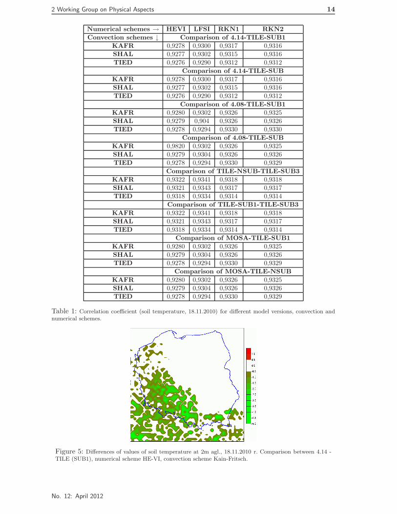
The worst results were received from experiment code v. 4.08, 4.14, MOSA, TILE VIEW(SUB1, NSUB, SUB3) of 18 November 2010 for the following combinations: 4.14 - TILE(SUB1), 4.14 - TILE (NSUB), 4.08 - TILE (SUB1), 4.08 - TILE (NSUB), TILE (NSUB) -TILE (SUB3), TILE (NSUB) - TILE (SUB3), TILE (SUB1) -TILE (SUB3), MOSA - TILE(SUB1), MOSA - TILE (NSUB) (Tab. 1, Fig. 5-7).

The best results have been received for numerical experiment using the code v. 4.08 and theMOSA version for February 1, 2009 and 18 November 2010, for all analyzed meteorologicalfields, and for February 1, 2009 using the TILE version with NSUB and with SUB1. Corre-lation coefficient was equal to 1 for all convection schemes. It suggests that meteorologicalfields are insensitive to soil processes parameterization regardless of numerical and of con-vection schemes applied.

No. 12: April 2012

2 Working Group on Physical Aspects 14

Numerical schemes → HEVI LFSI RKN1 RKN2

Convection schemes ↓ Comparison of 4.14-TILE-SUB1

KAFR 0,9278 0,9300 0,9317 0,9316

SHAL 0,9277 0,9302 0,9315 0,9316

TIED 0,9276 0,9290 0,9312 0,9312

Comparison of 4.14-TILE-SUB

KAFR 0,9278 0,9300 0,9317 0,9316

SHAL 0,9277 0,9302 0,9315 0,9316

TIED 0,9276 0,9290 0,9312 0,9312

Comparison of 4.08-TILE-SUB1

KAFR 0,9280 0,9302 0,9326 0,9325

SHAL 0,9279 0,904 0,9326 0,9326

TIED 0,9278 0,9294 0,9330 0,9330

Comparison of 4.08-TILE-SUB

KAFR 0,9820 0,9302 0,9326 0,9325

SHAL 0,9279 0,9304 0,9326 0,9326

TIED 0,9278 0,9294 0,9330 0,9329

Comparison of TILE-NSUB-TILE-SUB3

KAFR 0,9322 0,9341 0,9318 0,9318

SHAL 0,9321 0,9343 0,9317 0,9317

TIED 0,9318 0,9334 0,9314 0,9314

Comparison of TILE-SUB1-TILE-SUB3

KAFR 0,9322 0,9341 0,9318 0,9318

SHAL 0,9321 0,9343 0,9317 0,9317

TIED 0,9318 0,9334 0,9314 0,9314

Comparison of MOSA-TILE-SUB1

KAFR 0,9280 0,9302 0,9326 0,9325

SHAL 0,9279 0,9304 0,9326 0,9326

TIED 0,9278 0,9294 0,9330 0,9329

Comparison of MOSA-TILE-NSUB

KAFR 0,9280 0,9302 0,9326 0,9325

SHAL 0,9279 0,9304 0,9326 0,9326

TIED 0,9278 0,9294 0,9330 0,9329

Table 1: Correlation coefficient (soil temperature, 18.11.2010) for different model versions, convection andnumerical schemes.

Figure 5: Differences of values of soil temperature at 2m agl., 18.11.2010 r. Comparison between 4.14 -TILE (SUB1), numerical scheme HE-VI, convection scheme Kain-Fritsch.

No. 12: April 2012

2 Working Group on Physical Aspects 15

Figure 6: As in Fig. 5. Comparison between TILE SUB1 and SUB3, numerical scheme Runge-Kutta,convection scheme Tiedtke - shallow convection.

Figure 7: As in Fig. 5. Comparison between MOSA - TILE NSUB, numerical scheme Runge-Kutta 2,convection scheme Tiedtke.

The analysis of data shows that surface temperature is the most sensitive of meteorologicalfield to MOSAIC and/or TILE parameterization (see tables 1-8). Correlation coefficientsfor this field are the lowest in comparison with correlation coefficients for others. It seemedthat synoptic situation of 18.11.2010 was a main reason of it. During this day the entirearea of Poland was under an influence of a warm front, which was accompanied by rain-fall causing high amount of moist in a surface layer of soil and, subsequently, changes inphysical properties of soil (e.g. thermal conductivity). It has caused soil surface temperatureto be very sensitive to applied parameterizations. The change of physical properties of soilaffected also on heat and moisture fluxes from soil surface to atmosphere and - indirectly -onother meteorological fields such as air temperature, dew point temperature and humidity.A sensitivity of these fields on the parameterizations of soil processes is smaller comparedto sensitivity of soil surface temperature. Changing numerical and convection schemes onecould not significantly affect results - differences in values of correlation coefficients was inthe range of 0.01 to 0.06.

A sensitivity of meteorological fields for MOSAIC and/or TILE parameterization dependson a synoptic situation that affects current weather conditions. When in a given area thereare homogeneous synoptic conditions meteorological fields are more sensitive to MOSAICparameterization with numeric schemes leapfrog and leapsemi. This sensitivity was not ob-

No. 12: April 2012

2 Working Group on Physical Aspects 16

served for Runge-Kutta schemes, regardless of the applied schema types. When there isnon-homogeneous set of meteorological conditions it was not stated explicitly which param-eterization has a more significant influence on meteorological fields.

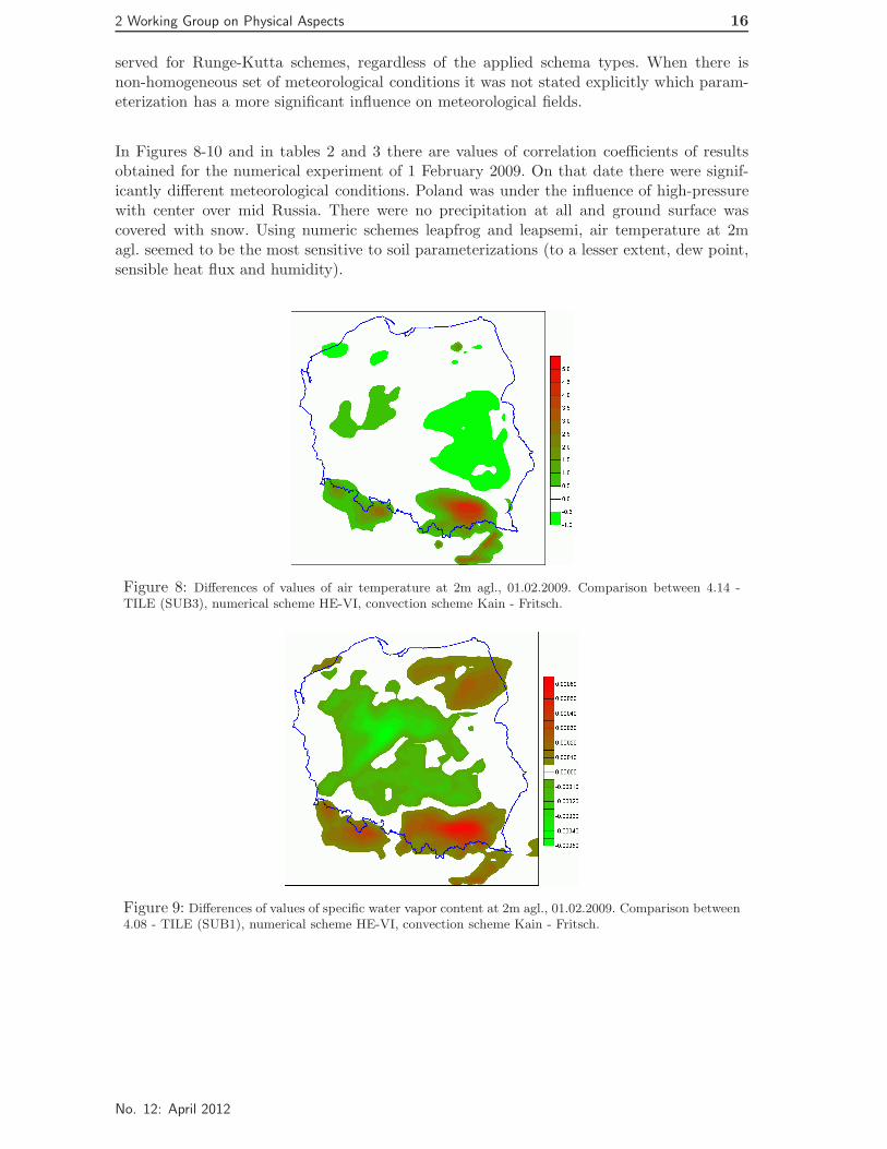
In Figures 8-10 and in tables 2 and 3 there are values of correlation coefficients of resultsobtained for the numerical experiment of 1 February 2009. On that date there were signif-icantly different meteorological conditions. Poland was under the influence of high-pressurewith center over mid Russia. There were no precipitation at all and ground surface wascovered with snow. Using numeric schemes leapfrog and leapsemi, air temperature at 2magl. seemed to be the most sensitive to soil parameterizations (to a lesser extent, dew point,sensible heat flux and humidity).

Figure 8: Differences of values of air temperature at 2m agl., 01.02.2009. Comparison between 4.14 -TILE (SUB3), numerical scheme HE-VI, convection scheme Kain - Fritsch.

Figure 9: Differences of values of specific water vapor content at 2m agl., 01.02.2009. Comparison between4.08 - TILE (SUB1), numerical scheme HE-VI, convection scheme Kain - Fritsch.

No. 12: April 2012

2 Working Group on Physical Aspects 17

Numerical schemes → HEVI LFSI RKN1 RKN2

Convection schemes ↓ Comparison of 4.14-TILE-SUB3

KAFR 0,9696 0,9708 0,9954 0,9954

SHAL 0,9699 0,9708 0,9954 0,9954

TIED 0,9711 0,9711 0,9972 0,9972

Comparison of 4.14-TILE-SUB1

KAFR 0,9677 0,9686 0,9986 0,9985

SHAL 0,9683 0,9688 0,9985 0,9985

TIED 0,9679 0,9673 0,9986 0,9986

Comparison of 4.14-TILE-NSUB

KAFR 0,9677 0,9686 0,9986 0,9985

SHAL 0,9683 0,9688 0,9985 0,9985

TIED 0,9679 0,9673 0,9986 0,9986

Comparison of 4.08-TILE-SUB3

KAFR 0,9695 0,9704 0,9939 0,9939

SHAL 0,9697 0,9706 0,9939 0,9939

TIED 0,9710 0,9710 0,9942 0,9943

Comparison of 4.08-TILE-SUB1

KAFR 0,9676 0,9684 0,9970 0,9970

SHAL 0,9682 0,9688 0,9970 0,9970

TIED 0,9679 0,9636 0,9960 0,9960

Comparison of 4.08 - TILE-NSUB

KAFR 0,9676 0,9684 0,9970 0,9970

SHAL 0,9682 0,9688 0,9970 0,9970

TIED 0,9679 0,9674 0,9960 0,9960

Comparison of TILE-NSUB - TILE-SUB3

KAFR 0,9800 0,9765 0,9949 0,9949

SHAL 0,9802 0,9774 0,9949 0,9949

TIED 0,9820 0,9786 0,9965 0,9965

Comparison of MOSAIC - TILE-SUB3

KAFR 0,9695 0,9704 0,9939 0,9939

SHAL 0,9697 0,9706 0,9939 0,9939

TIED 0,9710 0,9710 0,9942 0,9943

Comparison of MOSAIC - TILE-SUB1

KAFR 0,9676 0,9684 0,9970 0,9970

SHAL 0,9682 0,9688 0,9970 0,9970

TIED 0,9679 0,9674 0,9960 0,9960

Table 2: Correlation coefficient (air temperature, 01.02.2009) for different model versions, convection andnumerical schemes.

Numerical schemes → HEVI-LFSI HEVI-RKN1 HEVI-RKN2 LFSI-RKN1 LFSI-RKN2 RKN1-RKN2

Convection schemes/fields ↓ Comparison of TILE-NSUB

KAFR-QV2M 0,9872 0,9713 0,9714 0,9782 0,9782 0,9999

KAFR-TE2M 0,9830 0,9655 0,9655 0,9579 0,9579 0,9999

SHAL-TE2M 0,9845 0,9660 0,9660 0,9578 0,9578 0,9999

TIED-TE2M 0,9823 0,9651 0,9655 0,9658 0,9658 0,9999

Comparison of TILE-SUB1

KAFR-QV2M 0,9872 0,9713 0,9714 0,9782 0,9782 0,9999

KAFR-TE2M 0,9830 0,9655 0,9655 0,9579 0,9579 0,9999

SHAL-TE2M 0,9845 0,9660 0,9661 0,9578 0,9578 0,9999

TIED-TE2M 0,9823 0,9655 0,9655 0,9658 0,9658 0,9999

Table 3: Correlation coefficient (for selected meteorological fields in 01.02.2009) TILE version, NSUB andSUB1), for selected convection and numerical schemes.

No. 12: April 2012

2 Working Group on Physical Aspects 18

5 Conclusions

In this article results of tests carried out using a new soil processes parameterizations -MOSAIC and TILE in COSMO model COSMO are presented. Tests were carried out withdifferent convection and numerical schemes to assess how parameterization(s) contributes toa forecast of meteorological fields or which one of them exhibits stronger influence. Statisti-cal analysis was carried out and an analysis of the differences between the results obtainedwith parameterizations MOSAIC or TILE switched on and off. Results were divided intotwo groups. The first group includes results with the highest correlation coefficient (so called”the best case”), and the other - results with lowest correlation coefficient (”the worst case”).Best case suggests that the parameterization MOSAIC or TILE does not affect (almost atall) the forecast. The ”worst case” is an opposite situation, describing strong influence ofparameterization an forecast.

The analysis shows that: (a) synoptic situation that determines a weather in a given area, isalso a main factor determining an influence of parameterization of soil processes on meteoro-logical field(s). The manner of this influence would be a topic of on-going tests at IMGW; (b)MOSAIC parameterization has a more significant influence on meteorological fields in thecase of homogeneous meteorological conditions prevailing in the area of interest and (c) inthe case of ”heterogeneous” weather, resulting in a diversification of physical characteristicsof the soil - such as variations in the coverage of the snow surface of the soil - one cannotexplicitly specify a schema for parameterization of the processes of soil that would have moresignificant influence on a meteorological field. At the moment detailed work on this issue isin progress.

References

[1] Ament, F., 2006: Energy and moisture exchange processes over heterogeneous land -surfaces in a weather prediction model. PhD thesis

[4] Doms, G. and U. Schattler, 2002: A Description of the Nonhydrostatic Regional ModelLM, Part I: Dynamics and Numerics, DWD.

[3] Doms, G., and J. Forstner, E. Heise, H. - J. Herzog, M. Raschendorfer, T. Reinhardt, B.Ritter, R. Schrodin, J. - P.Schulz, G. Vogel, 2007: A Description of the NonhydrostaticRegional Model LM, Part II: Physical Parameterization, DWD.

[4] Schattler, U. and G. Doms, C. Schraff, 2009: A Description of the Nonhydrostatic Re-gional Model LM, Part VII: User’s Guide, DWD.

[5] Ament, F. and C Simmer, 2010: Improved Representation of Land - Surface Hetero-geneity in a Non - Hydrostatic Numerical Weather Prediction Model (personal commu-nication).

[6] Ament, F., 2008: COSMO SUBS. MeteoSwiss.

[7] Stensrud, D. J., 2007: Parameterization Schemes - Keys to Understanding NumericalWeather Prediction Models. Cambridge University Press.

[8] Cotton, W. R. and R. A. Anthes, 1989: Storm and Cloud Dynamics. Academic Press,INC.

No. 12: April 2012

2 Working Group on Physical Aspects 19

[9] Smith, R. K., 1997: The Physics and Parameterization of Moist Atmospheric Convec-tion. Kluwer Academic Publishers.

[10] Louis, J. F. , 1979: A parameterizartion model of vertical eddy fluxes in the atmosphere.Boundary Layer Meteorol. 17. 187 - 202.

[11] Tiedtke, M., 1989: A comprehensive mass flux scheme for cumulus parameterization inlarge scale model. Mon. Wea. Rev., pp. 1779 - 1800.

[12] Jacobson, M. Z., 2000: Fundamentals of Atmosferic Modeling. Cambridge UniversityPress.

[13] www.wetter3.de/fax - synoptic maps.

[14] Mellor, G. and T. Hamada, 1982: Development of a turbulence closure model for geo-physical fluid problem. Rev. Geophys. and Space Phys., 20, 851 - 875.

[15] Mellor, G. and T. Hamada, 1974: A hierarchy of turbulence closure models for planetaryboundary layers. J. Atm. and Space Phys., 31, 1791 - 1806.

[16] Rewut, I. B., 1980: Soil physics (in Polish: Fizyka gleby), PWRiL.

[17] Duniec, G. and A. Mazur, 2011: COLOBOC - MOSAIC parameterization in COSMOmodel v. 4.8. COSMO Newsletter, no. 11, 69 - 81.

[18] Warner, T. T., 2011: Numerical Weather and Climate Prediction. Cambridge UniversityPress.

No. 12: April 2012