
TECHNICAL MANUAL 1002 - State
82
New Jersey Department of Environmental Protection Division of Air Quality Technical Manual 1002 Guidance on Preparing an Air Quality Modeling Protocol May 2021
Transcript of TECHNICAL MANUAL 1002 - State

New Jersey Department of Environmental Protection
Division of Air Quality
Technical Manual 1002
Guidance on Preparing an Air Quality
Modeling Protocol
May 2021


i
Table of Contents
1.0 Introduction ............................................................................................................................................................. 1
1.1 Purpose of Document ................................................................................................................................... 1
1.2 Purpose of an Air Quality Impact Analysis .................................................................................................. 2
2.0 Sources Requiring Air Quality Impact Analysis...................................................................................................... 3
2.1 New Jersey Regulations and Modeling Analysis ......................................................................................... 3
2.1.1 Title V Operating Permits ........................................................................................................................ 3
2.1.2 Permits and Certificates for Minor Facilities and Major Facilities without an Operating Permit ............ 5
2.2 Sources That Must Conduct a Modeling Analysis ....................................................................................... 5
2.3 Netting Analysis and the Requirements for Modeling ................................................................................. 6
3.0 Regulatory Requirements ........................................................................................................................................ 7
3.1 National and New Jersey Ambient Air Quality Standards ........................................................................... 7
3.1.1 National Ambient Air Quality Standards (NAAQS) ............................................................................... 7
3.1.2 New Jersey Ambient Air Quality Standards (NJAAQS) ......................................................................... 8
3.2 Modeling Recommendations for Individual Criteria Pollutants ................................................................... 9
3.2.1 Federal Recommendations ....................................................................................................................... 9
3.2.2 New Jersey Recommendations .............................................................................................................. 10
3.3 Prevention of Significant Deterioration (PSD) Increments ........................................................................ 10
4.0 Basic Steps of an Air Quality Impact Analysis ..................................................................................................... 12
4.1 Modeling Protocol ...................................................................................................................................... 12
4.1.1 Preliminary (Single-Source) Modeling Protocol ................................................................................... 12
4.1.2 Multisource Modeling Protocol ............................................................................................................. 13
4.2 Preliminary (Single-Source) Modeling Analysis ....................................................................................... 13
4.2.1 Prediction of Insignificant Impact .......................................................................................................... 15
4.2.2 Prediction of Significant Impact in Attainment Areas ........................................................................... 15
4.2.3 Prediction of Significant Impact in Nonattainment Areas ..................................................................... 15
4.3 Multisource Modeling Analysis ................................................................................................................. 16
5.0 Model Selection ..................................................................................................................................................... 18
5.1 Screening Models ....................................................................................................................................... 18
5.1.1 CTSCREEN Model................................................................................................................................ 18
5.1.2 AERSCREEN Model ............................................................................................................................. 19
5.2 Refined Models .......................................................................................................................................... 19
5.2.1 AERMOD Model ................................................................................................................................... 19
5.2.2 CALPUFF Model .................................................................................................................................. 19
5.2.3 CTDMPLUS Model ............................................................................................................................... 20
6.0 Project Description and Site Characteristics .......................................................................................................... 21

ii
6.1 Project Overview ........................................................................................................................................ 21
6.2 Facility Plot Plan ........................................................................................................................................ 22
6.3 Good Engineering Practice (GEP) Stack Height Analysis ......................................................................... 23
6.4 Urban/Rural Determination ........................................................................................................................ 24
6.4.1 Land Use Analysis ................................................................................................................................. 25
6.4.2 Population Density Procedure ................................................................................................................ 27
6.5 Topography ................................................................................................................................................ 27
7.0 Emissions and Source Data ................................................................................................................................... 29
7.1 Emissions ................................................................................................................................................... 29
7.1.1 Partial Load and Startup/Shutdown Emissions ...................................................................................... 30
7.1.2 Fugitive Emissions ................................................................................................................................. 30
7.2 Types of Emission Sources ........................................................................................................................ 30
7.2.1 Point Sources ......................................................................................................................................... 30
7.2.2 Area Sources .......................................................................................................................................... 31
7.2.3 Volume Sources ..................................................................................................................................... 31
7.2.4 Roadways and Line Sources .................................................................................................................. 32
7.2.5 Flares ..................................................................................................................................................... 32
8.0 Establish Background Air Quality Concentrations ................................................................................................ 34
8.1 Sources of Background Air Quality Data ................................................................................................... 34
8.2 Use of Background Values in the Modeling Analysis ............................................................................... 37
8.2.1 Deterministic NAAQS and NJAAQS .................................................................................................... 37
8.2.2 Statistical Based NAAQS ...................................................................................................................... 37
8.2.2.1 1-Hour NO2 ..................................................................................................................................................................................................... 37
8.2.2.2 1-Hour SO2 ...................................................................................................................................................................................................... 38
8.2.2.3 24-Hour and Annual PM2.5.................................................................................................................................................................. 39
9.0 Receptor Network and Meteorological Data ................................................................................................... 41
9.1 Receptor Network ...................................................................................................................................... 41
9.2 Ambient Air ............................................................................................................................................... 41
9.3 Meteorological Data ................................................................................................................................... 42
10.0 Health Risk Assessments and Other Special Modeling Considerations .............................................................. 45
10.1 Health Risk Assessment ............................................................................................................................. 45
10.2 Cooling Towers .......................................................................................................................................... 47
10.3 Coastal Fumigation .................................................................................................................................... 47
10.4 Proximity to Major Sources ....................................................................................................................... 48
10.5 Use of Running Averages and Block Averages ......................................................................................... 48
10.6 Nitrogen Oxide to Nitrogen Dioxide Conversion ...................................................................................... 48
10.7 Treatment of Horizontal Stacks and Rain Caps.......................................................................................... 50
11.0 Air Quality Modeling Results .......................................................................................................................... 52
11.1 Modeling Submitted in Support of a New Jersey Air Permit Application ................................................. 52

iii
11.2 PSD Permit Applications ........................................................................................................................... 52
11.3 Documentation ........................................................................................................................................... 53
12.0 References ....................................................................................................................................................... 54
APPENDIX A ............................................................................................................................................................. 56
Additional Issues for PSD Affected New or Modified Sources................................................................................... 56
APPENDIX B .............................................................................................................................................................. 67
Example Air Quality Analysis Checklist ..................................................................................................................... 67
APPENDIX C .............................................................................................................................................................. 69
Odor Modeling Procedures .......................................................................................................................................... 69
List of Tables
2-1 Major Facility Thresholds 4
2-2 Significant Net Emissions Increase Thresholds-------------------------------------------------- 4
3-1 National Ambient Air Quality Standards --------------------------------------------------------- 7
3-2 New Jersey Ambient Air Quality Standards ------------------------------------------------------ 8
3-3 PSD Allowable Increments 11
4-1 Class I and Class II Area Significant Impact Levels ------------------------------------------- 14
4-2 Significant Air Quality Impact Levels for Increases in
Ambient Air Concentrations in Nonattainment Areas ----------------------------------------- 16
6-1 Identification and Classification of Land Use --------------------------------------------------- 25
7-1 Point Source Emission Input Data for NAAQS Compliance Demonstration -------------- 29
7-2 Suggested Procedures for Estimating σyO and σzO --------------------------------------------------------------------32
8-1 List of Pollutants Monitored at Each Site -------------------------------------------------------- 35
9-1 ASOS Meteorological Stations 43
10-1 Risk Management Guideline for Air Toxics ---------------------------------------------------- 47
A-1 Significant Monitoring Concentrations ---------------------------------------------------------- 56
A-2 Soils and Vegetation Screening Values ---------------------------------------------------------- 60
A-3 PSD Class I Significant Impact Levels and PSD Increments --------------------------------- 63
C-1 Conversion Factors for Peak-To-Mean Ratio --------------------------------------------------- 71
C-2 Published Odor Thresholds 72

iv
List of Figures
6-1 Correlation of USGS Land Cover Classifications with Auer Land Use Types ------------ 26
8-1 Locations of NJDEP Air Monitoring Sites ------------------------------------------------------ 36
9-1 Location of ASOS Meteorological Stations ----------------------------------------------------- 44
A-1 Required Receptor Locations in Brigantine Division of the E.B. Forsythe
National Wildlife Refuge 66

v
LIST OF ACRONYMS
The following are acronyms used in Technical Manual 1002.
amsl Above mean sea level
APC Air Pollution Control
AQRV Air Quality Related Value
BID Buoyancy-induced Dispersion
BPIPPRM Building Profile Input Program with the Plume Rise Model
CAA Clean Air Act
CFR Code of Federal Regulations
CMSA Consolidated Metropolitan Statistical Area
DAQ Division of Air Quality
DEM Digital Elevation Model
Department New Jersey Department of Environmental Protection
FLM Federal Land Manager
GEP Good Engineering Practice
HAP Hazardous Air Pollutant
ISC3 Industrial Source Complex (Version 3)
ISR In-stack ratio
MCHISRS Model Clearinghouse Information Storage and Retrieval System
MSA Metropolitan Statistical Area
NAAQS National Ambient Air Quality Standard
NJAAQS New Jersey Ambient Air Quality Standard
NJDEP New Jersey Department of Environmental Protection
NED National Elevation Dataset
N.J.A.C. New Jersey Administrative Code NO2 Nitrogen dioxide
NWS National Weather Service
PM10 Particulate matter having an aerodynamic diameter less than or equal to a
nominal 10 micrometers
PM2.5 Particulate matter having an aerodynamic diameter less than or equal to a
nominal 2.5 micrometers
ppb Parts per billion
ppm Parts per million
PSD Prevention Significant Deterioration
SCRAM Support Center for Regulatory Atmospheric Modeling
SIA Significant Impact Area
SMC Significant Monitoring Concentration SO2 Sulfur dioxide
TEOM Tapered element oscillating microbalance
TSP Total Suspended Particulates
USEPA United States Environmental Protection Agency
µg/m3 Micrograms per cubic meter
USGS United States Geological Survey

vi

1
1.0 Introduction
1.1 Purpose of Document
Air dispersion modeling is the primary analytical tool for assessing air quality impacts from new
or modified pollution sources when time, expenses and coverage limit the use of ambient air
measurement. The New Jersey Department of Environmental Protection (NJDEP) Division of
Air Quality (DAQ) has produced this Technical Manual (Manual) to provide modeling guidance
for predicting the ambient air quality impact of emissions from stationary sources. This Manual
addresses modeling issues for a wide range of source types and regulatory modeling
requirements, such as Prevention of Significant Deterioration (PSD). It is intended for use by
permit applicants and their consultants who need to conduct ambient impact analyses in support
of air permit applications and other activities that require air quality impact modeling.
This Manual is not intended to describe the implications of modeling results. Such implications
are generally controlled by relevant state and federal regulations, laws, and guidance documents.
This Manual is not intended to provide an all-inclusive description of the requirements of a
modeling analysis because each modeling analysis is unique. There can be many variations in
source configuration and operating characteristics and differences in geography and climate from
one modeling application to another. There is no one single model or methodology that can
assess all the conceivable modeling situations. The purpose of this Manual is to provide a
general framework for how the modeling analysis should be conducted, and to promote
technically sound and consistent modeling techniques while encouraging the use of improved
and more accurate techniques as they become available.
Individuals responsible for conducting the air quality impact analyses should, at a minimum, be
familiar with the following United States Environmental Protection Agency (USEPA)
documents:
• Appendix W to 40 CFR Part 51 – Guideline on Air Quality Models
• AERMOD Implementation Guide, EPA-454/B-16-013
• AERMOD User’s Guide, EPA-454/B-16-011
• AERSURFACE User’s Guide, EPA-454/B-08-001 (Revised 01/16/2013)
• AERMET User’s Guide, EPA-454/B-16-010
• Guideline for Determination of Good Engineering Practice Stack Height (Technical
Support Document for the Stack Height Regulations), EPA-450/4-80-023R
• Additional guidance from the USEPA Support Center for Regulatory Atmospheric
Modeling (SCRAM) at http://www.epa.gov/scram/ . Within SCRAM is the Model
Clearinghouse Information Storage and Retrieval System (MCHISRS) at
http://cfpub.epa.gov/oarweb/MCHISRS . It is a database of Model Clearinghouse

2
memoranda addressing the interpretation of modeling guidance for specific regulatory
applications.
As stated above, each modeling analysis is unique. Therefore, applicants should work closely
with the modeling staff at the Department to ensure that all modeling requirements are met. The
contact phone number is (609) 292-6722. Additional information can be obtained from the air
quality permit program’s webpage: http://www.nj.gov/dep/aqpp/ . Note that the results of air
dispersion modeling are used as inputs to risk assessment. New Jersey Technical Manual 1003
entitled “Guidance on Preparing a Risk Assessment for Air Contaminant Emissions” addresses
the preparation of risk assessments and is available on the Department’s webpage
http://www.state.nj.us/dep/aqpp/techman.html .
1.2 Purpose of an Air Quality Impact Analysis
An air quality impact analysis is used to establish compliance with the National Ambient Air
Quality Standards (NAAQS), the New Jersey Ambient Air Quality Standards (NJAAQS), and
the PSD allowable increments. An air quality impact analysis may also be required for:
• Assessing whether a source is causing “air pollution,” which is defined under New Jersey
Administrative Code (N.J.A.C.) Title 7 Chapter 27 Subchapter 5 (7:27-5) as the presence
in the outdoor atmosphere of one or more air contaminants in such quantities and
duration as are, or tend to be, injurious to human health or welfare, animal or plant life or
property, or would unreasonably interfere with the enjoyment of life or property. This
type of analysis usually involves a risk assessment (carcinogenic and non-carcinogenic
health effects) or an odor impact evaluation (see Appendix C, Odor Modeling
Procedures).
• Assessing Air Quality Related Values (AQRV), such as visibility, soils and vegetation
impacts that would occur as a result of the source, and general commercial, residential,
industrial and other growth associated with the source, as required by 40 CFR 52.21(o) of
the PSD regulations. This analysis should not only address impact on visibility, soils and
vegetation for the Brigantine Division of the Edwin B. Forsythe National Wildlife Refuge
Class I area, but also evaluate impacts to Class II areas that have a significant commercial
and recreational value.

3
2.0 Sources Requiring Air Quality Impact Analysis
2.1 New Jersey Regulations and Modeling Analysis
The New Jersey regulations that address the issue of air quality modeling are found in the
N.J.A.C. 7:27-8 (Permits and Certificates for Minor Facilities and Major Facilities without an
Operating Permit), 18 (Emission Offset Rules), and 22 (Operating Permits).
2.1.1 Title V Operating Permits
Most sources that will need to submit modeling analysis in support of their permit applications
will be those sources requiring a Title V operating permit. N.J.A.C. 7:27-22.8 sets forth the
requirements for submitting a modeling analysis for the following types of permit applications or
modifications: (1) a new major source requesting an initial Title V permit; (2) a significant
modification to an existing major facility; (3) or a minor modification to an existing major
facility.
Though there are four scenarios listed in N.J.A.C. 7:27-22.8(a) that require modeling analysis as
part of a Title V permit application or modification, only three of the principal concerns are
described in more detail below.
1. 22.8(a)1 - The criteria for determining whether an application is subject to the PSD air
quality impact analysis requirements can be found in 40 CFR Part 52.21(m). (Attainment)
2. 22.8(a)2 - An application is subject to the air quality impact analysis requirements set
forth at N.J.A.C. 7:27-18.4 if it is proposing an emissions increase, based on potential to
emit, that exceeds any of the major facility thresholds listed in Table 2-1 for at least one
pollutant. An air quality impact analysis must be conducted for an existing major facility
proposing a net emissions increase exceeding the thresholds listed in Table 2-2 below, as
determined pursuant to N.J.A.C. 7:27-18.7. (Nonattainment)
Additionally, Total Suspended Particulates (TSP) is not in Table 2-2 because the
Department assumes that if the NAAQS for particulate matter equal to or less than 10
microns (PM10) and the particulate matter equal to or less than 2.5 microns (PM2.5) are
met, then the TSP NJAAQS will also be met.
The USEPA November 17, 2016 Memo titled Draft PM2.5 Precursor Demonstration
Guidance requires that sulfur dioxide (SO2), oxides of nitrogen (NOx), VOC, and
ammonia must be evaluated in the development of all PM2.5 nonattainment area State
Implementation Plans. While New Jersey is currently attaining PM2.5 NAAQS, the
Department may require applicants to address VOC and ammonia as PM2.5 precursors.

4
Table 2-1. Major Facility Thresholds
Air Contaminant Threshold Value
(tons/yr) SO2 100
SO2 (as PM2.5 precursor) 100b
TSP 100 PM10 100 PM2.5 100a
CO 100
NOx 25 NOx (as PM2.5 precursor) 100b
VOC 25
Pb 10
a. This value reflects 40 CFR Part 51 Appendix S guidance.
b. Per revision to N.J.A.C. 7:27-18, adoption published in November 6, 2017 New Jersey Register.
Table 2-2. Significant Net Emissions Increase Thresholds
Air Contaminant Significant Net Emissions Increase
(tons/yr) SO2 40
SO2 (as PM2.5 precursor) 40b PM10 15
PM2.5 10a NOx 25
NOx (as PM2.5 precursor) 40b
CO 100
Pb 0.6
a. This value reflects 40 CFR Part 51 Appendix S guidance.
b. Per revision to N.J.A.C. 7:27-18, adoption published in November 6, 2017 New Jersey Register.
3. 22.8(a)4 - New and modified sources at major facilities with operating permits may need
to submit a health risk assessment if they emit certain contaminants regarded as air
toxics. Air toxics are natural or man-made pollutants that when emitted into the air may
cause an adverse health effect (see section 10.0 for health risk assessment modeling
recommendations). The federal 1990 Clean Air Act (CAA) Amendments created a list of
air toxics, called “hazardous air pollutants” or “HAPs”, as well as regulations to limit
HAP emissions. Air toxics that must be evaluated are listed on the NJDEP Division of
Air Quality Risk Screening Worksheet (Worksheet), which can be accessed at
http://www.state.nj.us/dep/aqpp/risk.html . The Worksheet evaluates HAPs, as well as
other air toxics, such as hydrogen sulfide and ammonia. Sources that require further
review per the Department’s risk screening procedures must conduct air quality
modeling, which applies site specific parameters to the assessment. The health risk
screening procedures are described in New Jersey Technical Manual 1003 (Guidance on
Preparing a Risk Assessment for Air Contaminant Emissions) and can be downloaded
from the Department’s air quality permitting program technical manual webpage at
http://www.state.nj.us/dep/aqpp/techman.html .

5
2.1.2 Permits and Certificates for Minor Facilities and Major Facilities without an
Operating Permit
The criteria for submission of a modeling analysis for minor facilities and major facilities
without an operating permit are specified in N.J.A.C. 7:27-8.5 (Air Quality Impact Analysis).
N.J.A.C. 7:27-8.5(a)1 and 2 are identical to the criteria for Title V operating permits set forth at
N.J.A.C. 7:27-22.8(a)1 and 2, respectively. As is the case with N.J.A.C. 7:27-22.8(a)4, most
sources affected by N.J.A.C. 7:27-8.5(b) will be those that require further review per the
Department’s risk screening procedure due to their emissions of air toxics, as listed in the
Worksheet. N.J.A.C. 7:27-8.5(a)4 is a catchall condition for permit applications that the
Department believes may cause or contribute to a violation of an ambient air quality standard or
a PSD increment, or pose a threat to public health or welfare, but are not subject to modeling
pursuant to any other criteria.
2.2 Sources That Must Conduct a Modeling Analysis
As required by 40 CFR Part 52, N.J.A.C. 7:27-8, and N.J.A.C. 7:27-22, an air quality modeling
analysis must be conducted under the following scenarios:
1. Applications subject to PSD air quality impact analysis requirements per 40 CFR Part
52.21(m) (see Appendix A for more details).
2. Applications for a new major source or an existing minor source proposing an emission
increase that exceeds the major source thresholds listed in Table 2-1 for at least one
pollutant. An air quality impact analysis must be conducted for each pollutant whose
proposed net emissions increase exceeds the thresholds listed in Table 2-2.
3. Applications for an existing major facility (allowable emissions above the levels in Table
2-1 for at least one pollutant) must conduct an air quality impact analysis for those
pollutants whose proposed net emissions increase exceed the thresholds listed in Table 2-
2.
4. Applicants that submit an APC permit where the Department’s risk screening procedure
indicates that further evaluation is required due to their emissions of air toxics.
5. The Department may request modeling in other unique circumstances. For instance,
circumstances could involve a permit application at a new or existing major facility that
the Department believes may cause or contribute to a violation of an ambient air quality
standard or a PSD increment, or pose a threat to public health or welfare. For example, if
a proposed increase in the hourly emission rate of a criteria pollutant is of sufficient
magnitude that, in combination with the source’s stack height, it may cause or contribute
to a violation of a short-term ambient air quality standard or a PSD increment, modeling
may be required even though the annual emissions increase may not be significant.
Another example is a minor facility with insufficient annual emissions to meet the major
facility threshold values in Table 2-1, but has a proposed emission increase and stack

6
parameters that suggest high air impacts. In this case, a new source proposing emissions
of 80 tons per year of PM10 would likely need to be modeled.
2.3 Netting Analysis and the Requirements for Modeling
A netting analysis is sometimes performed pursuant to N.J.A.C. 7:27-18 when obtaining an air
permit for a new or modified source. By accounting for creditable emissions reductions, the net
emissions increase at a facility for a pollutant may be reduced below levels outlined in the
Emissions Offset Rule. The methodology for calculating the net emissions increase at a facility
is described in N.J.A.C. 7:27-18.7 (Determination of a net emissions increase or a significant net
emissions increase).
A netting analysis can reduce the emissions increase at the facility below the significant net
emissions increase threshold for which an air quality impact analysis is required. An exemption
from performing a modeling analysis can be requested in such a situation. The exemption
request may be denied if the Department believes that the reduction in ambient air concentrations
from the emissions decrease will not be sufficient to prevent the proposed emissions increase
from causing or contributing to a violation of an ambient air quality standard or a PSD
increment, or posing a threat to public health or welfare. Proposed emission increases from a
source located near complex terrain, near the property boundary line of the facility, in an area
where elevated background air concentrations exist, or a stack subject to building downwash are
examples of situations where a requested exemption from modeling may be denied.
While the air dispersion modeling is dependent upon the netting analysis as described by
N.J.A.C. 7:27-18.7, it is a separate regulatory demonstration. When modeling a source for which
a netting analysis has been conducted, an applicant should include not only the proposed
emissions increases, but also the creditable emissions reductions at the source. Please note that
the modeling of negative nitrogen dioxide (NO2) emissions should only be done after
consultation with the USEPA Regional Office to ensure that decreases are not overestimated.

7
3.0 Regulatory Requirements
The permit applicant must demonstrate compliance with the federal and the New Jersey air
quality regulations. Below is a summary of the applicable regulatory requirements that are
related to air quality modeling procedures and results.
3.1 National and New Jersey Ambient Air Quality Standards
3.1.1 National Ambient Air Quality Standards (NAAQS)
Congress enacted the 1970 Clean Air Act (CAA) to protect the health and welfare of the public
from the adverse effects of air pollution. Subsequently, the USEPA established National
Ambient Air Quality Standards (NAAQS) for six criteria pollutants: sulfur dioxide (SO2),
particulate matter (PM10 and PM2.5), nitrogen dioxide (NO2), carbon monoxide (CO), ozone (O3),
and lead (Pb). The NAAQS include both “primary” and “secondary” standards and are
periodically updated to reflect the latest scientific findings. The primary standards are intended
to protect human health with an adequate margin of safety; whereas the secondary standards are
intended to protect public welfare from any known or anticipated adverse effects associated with
the presence of air pollutants, such as damage to materials or vegetation. Both the primary and
the secondary standards must be addressed in the modeling evaluation. Table 3-1 “National
Ambient Air Quality Standards” lists these primary and secondary standards.
Table 3-1. National Ambient Air Quality Standards
Pollutant
Averaging
Perioda
Primary
NAAQSb
Secondary
NAAQSb
NO2
1-hour 3
100 ppb (188 μg/m ) ---
Annual 3
53 ppb (100 μg/m ) 3
53 ppb (100 μg/m )
CO 1-hour
3
35 ppm (40,000 μg/m ) ---
8-hour 3
9 ppm (10,000 μg/m ) ---
SO2
1-hour 3
75 ppb (196 μg/m ) ---
3-hour --- 3
0.5 ppm (1,300 μg/m )
PM10 24-hour 3
150 μg/m 3
150 μg/m
PM2.5
24-hour 3
35 μg/m 3
35 μg/m
annual 3
12 μg/m 3
15 μg/m
Ozone 8-hour 0.070 ppm 0.070 ppm
Lead Rolling 3-month 3
0.15 μg/m 3
0.15 μg/m
a. Short-term standards for 3-hour SO2 and 1- and 8-hour CO are not to be exceeded more than once per year. The 3-month lead and annual NO2 standards are never to be exceeded. The 1-hr NO2 standard is the 98th percentile of the yearly distribution of 1-hour daily maximum concentrations averaged over 3 years. The 1-hr SO2 standard is the 99th percentile of the yearly distribution of 1-hour daily maximum concentrations averaged over 3 years. The 24-hr PM10 standard is not to be exceeded more than once per year over 3 years. The 24-hr PM2.5 standard is the 98th percentile of the maximum averaged over 3 years, and the annual PM2.5 standards are annual means averaged over 3 years.

8
b. The actual form of each standard is listed first. The values in parentheses are approximations provided
for convenience.
3.1.2 New Jersey Ambient Air Quality Standards (NJAAQS)
New Jersey Ambient Air Quality Standards (NJAAQS) are listed in Table 3-2. The differences
between the New Jersey and the National standards are as follows:
• New Jersey maintains a 12-month and a 24-hour secondary standard for SO2;
• New Jersey maintains 12-month and 24-hour primary and secondary standards for Total
Suspended Particulates (TSP);
• New Jersey has no standards for PM2.5 and PM10; and
• New Jersey regulations specify its 3-hr, 8-hr, and 24-hr standards in terms of moving or
non-overlapping running hourly averages, and its 3-month and 12-month standards in
terms of moving or non-overlapping running monthly averages.
Table 3-2. New Jersey Ambient Air Quality Standards
Pollutant
Averaging
Perioda
Primary
NJAAQSb
Secondary
NJAAQSb
NO2 12-Month 3
100 μg/m (0.05 ppm) 3
100 μg/m (0.05 ppm)
CO 1-hour
3
40 mg/m (35 ppm) 3
40 mg/m (35 ppm)
8-hour 3
10 mg/m (9 ppm) 3
10 mg/m (9 ppm)
SO2
3-hour --- 3
1,300 μg/m (0.5 ppm)
24-hour 3
365 μg/m (0.14 ppm) 3
260 μg/m (0.10 ppm)
12-Month 3
80 μg/m (0.03 ppm) 3
60 μg/m (0.02 ppm)
TSP 24-hour
3
260 μg/m 3
150 μg/m
12-Month 3
75 μg/m 3
60 μg/m
Ozone 1-hour 0.12 ppm 0.08 ppm
Lead 3-month 3
1.5 μg/m 3
1.5 μg/m
a: All short-term (1-hr, 3-hr, 8-hr, and 24-hr) standards except ozone are not to be exceeded more than once
per 12-month period. 3-month and 12-month standards are never to be exceeded. All averages are
calculated as running or moving averages. The 12-month TSP standards are geometric means.
b: The actual form of each standard is listed first. The values in parentheses are approximations provided
for convenience.

9
3.2 Modeling Recommendations for Individual Criteria Pollutants
3.2.1 Federal Recommendations:
Guidance on how to demonstrate compliance with the NAAQS is given in 40 CFR 51 Appendix
W Section 9.2.3 (NAAQS and PSD Increments). The following is additional guidance on
demonstrating NAAQS compliance for specific pollutants.
NO2
The 1-hour NO2 NAAQS is a probabilistic standard. Compliance is demonstrated as the 98th
percentile of the 1-hour daily maximum concentration averaged over 3 years, which is equivalent
to the 8th highest of the annual distribution of the daily maximum 1-hour concentrations averaged over five years. If three years of prognostic meteorological data are modeled, then the 8th highest
of the annual distribution of the daily maximum 1-hour NO2 concentrations is averaged over
three years. And, finally, if one year of site-specific meteorological data is modeled, simply the 8th highest of the daily maximum 1-hour concentrations should be used for comparison to the
NAAQS.
The following USEPA guidance memorandums provide additional information for demonstration with the 1-hour NO2 standard: Clarification on the Use of AERMOD Dispersion
Modeling for Demonstrating Compliance with the NO2 National Ambient Air Quality Standard
(dated September 30, 2014), and Additional Clarification Regarding Application of Appendix W Modeling Guidance for the 1-Hour NO2 National Ambient Air Quality Standard (dated March 1,
2011).
Ozone and Secondarily Formed Particulate Matter
A modeling analysis showing compliance of an individual source with the ozone NAAQS is
generally not required. Draft guidance for assessing secondary impacts was provided in the
USEPA memorandum, Guidance on the Development of Modeled Emission Rates for Precursors
(MERPs) as a Tier 1 Demonstration Tool for Ozone and PM2.5 under PSD Permitting Program
(dated December 2, 2016).
PM2.5
Major PM2.5 sources or major modifications (as defined by the USEPA) should follow the
USEPA Implementation of the New Source Review Program for Particulate Matter Less Than
2.5 Micrometers, Final Rule (May 16, 2008 Federal Register) and 40 CFR Part 51, Appendix S,
for nonattainment compliance demonstrations. Additional guidance for demonstrating
compliance with the PM2.5 NAAQS and PSD Increments is provided in the USEPA
Memorandum Guidance for PM2.5 Permit Modeling (dated May 20, 2014).
PM10
The 24-hour PM10 NAAQS is a probabilistic standard. The standard is not to be exceeded more
than once per year over an average of 3 years. When multiple years are modeled, they
collectively represent a single period. Thus, if five years of NWS data are modeled, then the
highest sixth highest concentration for the whole period becomes the design value.

10
SO2
The 1-hour SO2 NAAQS is a probabilistic standard. Compliance is demonstrated as the 99th
percentile of the 1-hour daily maximum concentration averaged over 3 years, which is equivalent to the fourth highest of the annual distribution of daily maximum 1-hour concentrations averaged
over five years. Just as in evaluating the 1-hour NO2 impact concentrations, if three years of
prognostic meteorological data are modeled, then the 4th highest of the annual distribution of the
daily maximum 1-hour SO2 concentrations is averaged over three years. And, finally, if one year
of site-specific meteorological data is modeled, simply the 4th highest of the daily maximum 1- hour SO2 concentrations should be used for comparison to the NAAQS.
The following USEPA guidance memorandums provide additional information for
demonstration with the 1-hour SO2 standard: Guidance Concerning the Implementation of the 1-
hour SO2 NAAQS for the Prevention of Significant Deterioration Program (dated August 23,
2010), and Additional Clarification Regarding Application of Appendix W Modeling Guidance
for the 1-Hour NO2 National Ambient Air Quality Standard (dated March 1, 2011).
Lead
On October 15, 2008, USEPA revised the lead NAAQS from 1.5 µg/m3 based on calendar
quarters to 0.15 µg/m3 based on a rolling 3-month average.
3.2.2 New Jersey Recommendations:
Many of the NJAAQS are identical to the NAAQS. However, the New Jersey rules specify its
3-hr, 8-hr, and 24-hr standards in terms of moving or running hourly averages, and its 3-month
and 12-month (annual) standards in terms of moving or running monthly averages. The NAAQS
are defined in terms of blocked averages, both for short-term (24-hours or less) and annual
averages. For example, when demonstrating compliance with a 24-hour NAAQS, pollutant
concentrations are calculated from midnight to midnight the next day. When demonstrating
compliance with a 24-hour NJAAQS, pollutant concentrations are calculated from midnight to
midnight, from 1 a.m. to 1 a.m. the next day, from 2 a.m. to 2 a.m. the next day, etc.
Initially, compliance with the NJAAQS can be based on use of block averages (similar to the
NAAQS). However, if the modeled impact based on blocked averages with representative
background concentration added exceeds 90% of the NJAAQS, compliance must then be based
on the running hourly and monthly averages for that pollutant and averaging time.
As with the ozone NAAQS, single-source ozone modeling to demonstrate compliance with the
ozone NJAAQS usually is not required due to the lack of modeling tools. Modeling of a
source’s total suspended particulate (TSP) impact generally is not required because the
Department assumes that if the PM10 and PM2.5 NAAQS are met, then the TSP NJAAQS will
also be met.
3.3 Prevention of Significant Deterioration (PSD) Increments
11
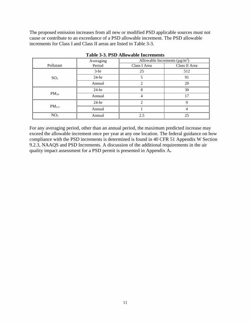
The proposed emission increases from all new or modified PSD applicable sources must not
cause or contribute to an exceedance of a PSD allowable increment. The PSD allowable
increments for Class I and Class II areas are listed in Table 3-3.
Table 3-3. PSD Allowable Increments
Pollutant
Averaging
Period
Allowable Increments (µg/m3)
Class I Area Class II Area
SO2
3-hr 25 512
24-hr 5 91
Annual 2 20
PM10
24-hr 8 30
Annual 4 17
PM2.5
24-hr 2 9
Annual 1 4
NO2 Annual 2.5 25
For any averaging period, other than an annual period, the maximum predicted increase may
exceed the allowable increment once per year at any one location. The federal guidance on how
compliance with the PSD increments is determined is found in 40 CFR 51 Appendix W Section
9.2.3, NAAQS and PSD Increments. A discussion of the additional requirements in the air
quality impact assessment for a PSD permit is presented in Appendix A.

12
4.0 Basic Steps of an Air Quality Impact Analysis
There are up to three major components in an air quality impact analysis – modeling protocols,
preliminary (single-source) modeling, and multisource modeling analysis. Each component is
described in the following sections.
4.1 Modeling Protocol
4.1.1 Preliminary (Single-Source) Modeling Protocol
In accordance with N.J.A.C. 7:27-8.5(d), 18.4(c), and 22.8(c), a modeling protocol must be
submitted and approved in advance by the Department before the air quality impact analysis
and/or a risk assessment is conducted. These regulations specify that the protocol address all
relevant general and site-specific factors and how the air quality impact analysis and/or risk
assessment will be conducted. N.J.A.C. 7:27-8.5(d), 18.4(c), and 22.8(c) all reference this
document and Technical Manual 1003 (Guidance on Preparing a Risk Assessment for Air
Contaminant Emissions) for guidance on preparing a modeling protocol.
The protocol should document in detail the methods the applicant proposes to conduct the
modeling analysis and present the results. The protocol must be received and approved by the
Department before a modeling analysis can be conducted and submitted. The Department will
not accept a modeling analysis that was performed without a pre-approved protocol.
In general, a modeling protocol should contain the following information:
• Project Description, including a project overview, facility plot plan, emissions, stack
parameters, and special operating and load scenarios, if necessary;
• Project Site Characteristics, including a land use analysis, attainment status, description
of the local topography, a Good Engineering Practice (GEP) stack height analysis, and
the meteorological data proposed for use in the modeling analysis;
• Regulatory Requirements, including a description of what federal and New Jersey
regulations and guidelines apply to the proposed project;
• Proposed Air Quality Analysis, including the proposed air quality model selection and
justification for use, screening analysis, and the proposed methods for refined modeling.
• Special Modeling Considerations, including the approach for addressing Class I area
modeling, such as the effects on soils and vegetation/growth analysis, near field and long-
range visibility, cooling tower modeling, coastal fumigation, health risk assessment,
fugitive emissions, deposition and odor modeling (see Appendix C, Odor Modeling
Procedures), if necessary;
• Establishing Background Air Quality, including justification of the background air
quality monitoring data to be used in the analysis; and

13
• Presentation of Air Quality Modeling Results, including how maximum impacts,
significant impact areas, and compliance with ambient air quality standards and PSD
increments will be demonstrated.
Appendix B of this document contains a summary checklist that can be used to assess the
completeness of an air quality modeling protocol and analysis. The Department recommends
that this checklist be reviewed by the applicant before the documents are submitted to the
Department. The modeling protocol should be submitted at the same time the air permit
application is sent to the Department. The permit engineer assigned to the project should be
informed that a modeling protocol has been submitted to the Department. The Department will
not review protocols until an air permit application is received by the Department. Paper copies
of modeling protocols and analyses should be sent to:
Chief, Air Quality Permitting
NJDEP, Division of Air Quality
P.O. Box 420 Mailcode 401-02
401 East State Street, 2nd Floor
Trenton, NJ 08625
4.1.2 Multisource Modeling Protocol
As discussed in Section 4.3 of this chapter, a multisource modeling analysis may be necessary if
preliminary single-source modeling shows that the proposed source has a significant impact. In
this situation, the applicant should submit an additional protocol known as a multisource
modeling protocol. A multisource modeling protocol should be submitted and approved by the
Department before an applicant conducts multisource modeling of nearby sources. The
multisource modeling protocol should include how the multisource inventory was generated,
information on the sources included in the multisource modeling, and the modeling methodology
that would be employed in the multisource analysis. The same air quality models and
meteorological data used in the preliminary (single-source) modeling of the proposed source are
normally used for the multisource analysis.
4.2 Preliminary (Single-Source) Modeling Analysis
The preliminary modeling analysis evaluates only the emissions from proposed new sources, or
the net emissions increase from a proposed modification.
Per PSD and New Source Review provisions in the 1990 Clean Air Act, one of the principal
functions of the preliminary modeling analysis is to determine whether emissions from proposed
new sources or the net emissions from a proposed modification will increase ambient
concentrations of that pollutant by more than the significant impact levels listed in Table 4-1.
The highest modeled pollutant concentration for each pollutant’s NAAQS and NJAAQS
averaging time is used to determine whether a source will have a significant impact, except for 1-
hr NO2, 1-hr SO2, 24-hr PM2.5, and annual PM2.5, where at least a 3-year average of the modeled
pollutant concentrations will be used to determine the significant impact.

14
When modeling a facility for which a netting analysis has been performed, the source’s proposed
emissions increases should be modeled first to determine if they will cause a significant impact.
If pollutants and averaging times from the proposed emissions increase are predicted to have
significant impact, additional refined modeling may be conducted to account for the effect of the
creditable emissions reductions at the facility. In this modeling analysis, the proposed emissions
increases should be modeled as positive emissions and the creditable emissions reductions at the
facility modeled as negative emissions.
The possibility of a significant impact in a Class I area must also be examined if the source
requires a PSD permit and is located within 100 kilometers (km) of a Class I area. In addition, if
the source is located within a 100 km of Class I area, a Class I increment demonstrated must be
included. PSD sources with large emissions that are located further than 100 km from a Class I
Area may need to examine their impact on the Class I area; This determination is made on a
case-by-case basis. Furthermore, all PSD source applicants should contact the Fish and Wildlife
Office in Denver, Colorado to determine if special Air Quality Related Values Analysis is
required for their new source or modification. Contact information is listed in Appendix A.
The only Class I area in or within 100 km of New Jersey is the Brigantine Division of the Edwin
B. Forsythe National Wildlife Refuge (see Figure A-1). If refined modeling shows that the
proposed PSD source has a significant impact in this Class I area, a multisource modeling
analysis is necessary to determine PSD increment consumption at the Class I area and possible
effects on its Air Quality Related Values (AQRVs). Further guidance on conducting a Class I
visibility and other AQRVs analyses is given in Appendix A.
Table 4-1. Class I and Class II Area Significant Impact Levels
Pollutant Averaging
Period
Significant Impact Levels (µg/m3)
Class I Area Class II Area
SO2
1-hour --- 7.8a
3-hr 1.0 25
24-hr 0.2 5
Annual 0.1 1
NO2 1-hour --- 10b
Annual 0.1 1
CO 1-hr --- 2,000
8-hr --- 500
PM2.5a 24-hr 0.27c 1.2
Annual 0.05c 0.2d
PM10 24-hr 0.3 5
Annuale 0.2 1
Pba 3-month --- 0.01
a. Maximum of 5-year average 1st highest maximum concentration.
b. NESCAUM interim significance level as maximum 1st high concentration (April 21, 2010 document);
USEPA has recommended 4ppb (~7.5 µg/m3) as maximum of 5-year average 1st highest maximum
concentration.
c. Revised 24-hour and annual PM2.5 Class I SIL per April 17, 2018 EPA guidance memo..
d. Revised annual PM2.5 Class II SIL of 0.2 µg/m3 per April 17, 2018 EPA guidance memo... e. Annual PM10 SILs are listed because annual increments still required.

15
4.2.1 Prediction of Insignificant Impact
When the significant impact levels (SILs) for each applicable pollutant at each applicable
averaging time are not exceeded, a multisource modeling analysis is usually not necessary.
There are circumstances when the reviewing authority (e.g., NJDEP and/or USEPA) may require
multisource modeling even if the predicted source impacts are less than the SILs (i.e., predicted
total impacts are within a significant impact level value of the NAAQS, and specifically for
PM2.5 modeling). For PSD permits, the applicant is required to demonstrate that allowable PSD
increments are not being consumed by way of multisource modeling. See Section 3.3 of this
document for additional information. Please note that the applicant must always demonstrate
compliance with the NAAQS and NJAAQS by adding the applicable background concentrations
to the appropriate modeled concentrations.
4.2.2 Prediction of Significant Impact in Attainment Areas
If predicted impacts are above the significant impact levels in an attainment area, then a
multisource modeling protocol as described in Section 4.1.2 and a multisource modeling analysis
as described in Section 4.3 will be required, and the project’s Significant Impact Area (SIA)
must be calculated. The SIA is a circular area with a radius extending from the source to the
most distant point where approved dispersion modeling predicts a significant ambient impact
will occur. The SIA should be determined for each pollutant and averaging period that has been
assigned a significant impact level.
4.2.3 Prediction of Significant Impact in Nonattainment Areas
The requirements of N.J.A.C. 7:27-18 (Emission Offset Rule) for Lowest Achievable Emission
Rate (LAER) and emission offsets will apply to the emissions of a criteria pollutant if the facility
is in an area that is in nonattainment for that criteria pollutant and the permit application is
subject to N.J.A.C. 7:27-18 pursuant to N.J.A.C. 7:27-18.2 for that criteria pollutant (discussed
in Section 2.1.1 and Tables 2-1 and 2-2 of this document). In addition, a permit application can
be subject to the LAER and offset requirements of N.J.A.C. 7:27-18 for a given criteria pollutant
when the facility is in an area that is in attainment for that criteria pollutant and the following
occurs:
1. The permit application is subject to N.J.A.C. 7:27-18 for that criteria pollutant and the
proposed net emissions increase would result in an increase in the ambient concentration
of the criteria pollutant in an area that is in nonattainment for that criteria pollutant; and
2. The increase in the ambient concentration of the criteria pollutant is equal to or exceeds
the significant air quality impact level specified in Table 4-2.
Thus, in some cases, the preliminary modeling analysis must include an evaluation of the permit
application’s proposed net emissions increase on any nearby nonattainment areas. All areas in
the State are designated as attainment for NO2, CO, TSP, PM2.5, PM10, and lead.

16
Table 4-2. Significant Air Quality Impact Levels for Increases in
Ambient Air Concentrations in Nonattainment Areas*
Pollutant Averaging Time
Annual 24-Hour 8-Hour 3-Hour 1-Hour
SO2 1.0 µg/m3 5 µg/m3 - 25 µg/m3 -
TSP 1.0 µg/m3 5 µg/m3 - - -
NO2 1.0 µg/m3 - - - -
CO - - 500 µg/m3 - 2000 µg/m3
Pb - 0.1 µg/m3 - - -
PM-10 1.0 µg/m3 5 µg/m3 - - -
* Per N.J.A.C. 7:27-18.4
The following areas are currently designated as nonattainment areas for New Jersey for the
following criteria pollutants:
Ozone
The entire state is classified as nonattainment for the 8-hr ozone standard (2008, 75 ppb), with
the New York-Northern New Jersey-Connecticut area classified as moderate and the
Philadelphia-Wilmington-Atlantic City area classified as marginal.
SO2
New Jersey is classified as nonattainment with the 1971 SO2 standard of 0.5 ppm for portions of
Warren County that include the following: the Township of Belvidere, the Township of
Harmony, portions of Liberty Township (south of UTM coordinate N4522 and west of UTM
coordinate E505), portions of Mansfield Township (west of coordinate E505), the Township of
Oxford, and the Township of White.
4.3 Multisource Modeling Analysis
When the impact from the proposed source or modification is significant in an attainment area, a
comprehensive assessment of air quality is obtained by performing a multisource modeling
analysis. The multisource modeling includes not only the facility obtaining the permit, but the
contribution from other nearby major sources as well as representative air monitoring data.
Those major sources that are located within or near the SIA of the proposed source or
modification should be included in the multisource modeling analysis. As mentioned earlier, if
the proposed source’s air quality impact requires a multisource modeling, the applicant must
submit a multisource modeling protocol for approval prior to performing the modeling analysis.
A major source is generally considered to be a facility with the potential to emit 100 or more tons
per year of the subject pollutant (0.6 ton per year or more for lead) and is located within or near
the SIA of the proposed source or modification. However, other sources with the potential to
emit less than 100 tons per year may need to be included in the modeling if they are located
within or near the SIA. For example, other sources emitting greater than 25 tons per year of NO2
and located within the SIA should be investigated for multisource modeling if the applying
source has a significant 1-hour NO2 impact. For applicants requiring a PSD permit, “near” is

17
considered to extend 10 to 20 km from the source(s) applying for a permit or modification. For
non-PSD sources, “near” usually extends to at least 10 km beyond the SIA. Each modeling
situation is unique; identification of nearby sources requires case-by-case professional
judgement. The final multisource modeling inventory may not necessarily be limited by or
inclusive of the sources initially investigated.
The applicant is responsible for developing the multisource modeling inventory. The
multisource modeling analysis usually consists of two separate evaluations: an evaluation of the
NAAQS and NJAAQS; as well as an evaluation of the PSD increments. Thus, two separate
modeling inventories may need to be developed. The modeling inventory needs to include the
emission units, emission rates, and stack parameters for each source included in the modeling
analysis. Building parameters may have to be included if the Department believes the downwash
effects are important in accurately predicting the source’s contribution to the multisource impact.
The Department will normally assist the applicant in identifying potential sources for inclusion
in the modeling. For those sources identified as potential candidates for inclusion in the
multisource modeling, a request can be made to the Department for a copy of their Title V
Operating Permit. The allowable emission rates and stack parameters can be obtained from the
Operating Permit. For proposed sources or modifications with significant impact areas that
approach or extend into an adjacent state, a similar type of inventory must be obtained from that
state as well. It is the responsibility of the applicant to obtain the necessary data from the other
state(s).
To simplify multisource inventory development, the Department suggests initially modeling
allowable emission rates. However, if necessary, modeling may account for actual operations for
nearby sources when demonstrating NAAQS and PSD increment compliance. Additional details
for developing an emission inventory are provided in the Revisions to the Guideline on Air
Quality Models: Enhancements to the AERMOD Dispersion Modeling System and Incorporation
of Approaches to Address Ozone and Fine Particulate Matter, Federal Register, January 17,
2017. Consultation with the Department is recommended when developing emission inventories.
In cases where many nearby major sources have been identified, the applicant may propose
screening techniques to limit the number of sources that are explicitly modeled. The multisource
modeling protocol should discuss the methodology used to eliminate these sources from the
analysis, such as concentration gradient modeling or adequate representation by background
ambient monitoring. The permit applicant must adequately justify the exclusion of nearby
sources from a multisource inventory. The applicant should obtain the Department’s agreement
on the methodology selected to remove sources from the inventory before submittal of the
multisource inventory.

18
5.0 Model Selection
There are two levels of sophistication of models used in an air quality modeling analysis. The
first level consists of relatively simple estimation techniques that generally use preset, worst-case
meteorological conditions to provide conservative estimates of the air quality impact of a
specific source, or source category. These are called screening techniques or screening models.
The second level consists of those analytical techniques that provide more detailed treatment of
physical and chemical atmospheric processes, require more detailed and precise input data, and
provide more specialized concentration estimates. As a result, they provide a more refined and
more accurate estimate of source impact and the effectiveness of control strategies. These are
referred to as refined models.
Several factors must be considered in the model selection process. These factors include source
type, pollutant averaging times that are to be addressed, the potential for aerodynamic building
downwash affecting the emissions, nearby terrain features and the existence of complex terrain
or complex wind flows, and the local urban/rural land use characteristics. The modeling protocol
should specify the models selected, their version numbers, and a justification for their use in the
air quality modeling analysis. The model options used in the analysis must be consistent with
those recommended by USEPA and approved by the Department.
5.1 Screening Models
A screening modeling analysis is sometimes conducted for the following reasons: (1) to provide
a preliminary indication of worst-case pollutant concentrations; (2) to identify the source’s
worst-case load or plant operating conditions that cause the highest ground-level concentrations;
(3) to assist in delineating the appropriate receptor grid for detailed or refined modeling; (4) to
determine a source’s impacts during equipment startup and shutdown; and (5) to determine the
impact of a source located in complex terrain for which no representative hourly meteorological
data is available.
5.1.1 CTSCREEN Model
CTSCREEN can be used to obtain conservative, yet realistic, estimates for receptors located on
terrain above stack height. CTSCREEN accounts for the three-dimensional nature of plume and
terrain interaction and requires detailed terrain data representative of the modeling domain.
CTSCREEN is the screening version of CTDMPLUS.
CTSCREEN is designed to execute a fixed matrix of meteorological values for wind speed,
standard deviation of horizontal and vertical wind speeds, vertical potential temperature gradient,
Monin-Obukhov length, mixing height as a function of terrain height, and wind directions for
both neutral/stable conditions and unstable convective conditions. CTSCREEN is designed to
address a single source scenario. Placement of receptors requires very careful attention when
modeling in complex terrain. Often the highest concentrations are predicted to occur under very
stable conditions, when the plume is near or impinges on the terrain.

19
5.1.2 AERSCREEN Model
AERSCREEN is the screening model whose algorithms are based on AERMOD. This model
will produce estimates of regulatory design concentrations without the need for on-site or five
years of National Weather Service (NWS) meteorological data and is designed to produce
concentrations that are equal to or greater than the estimates produced by AERMOD with a fully
developed set of meteorological and terrain data. It will make predictions in both simple and
complex terrain for a single source.
5.2 Refined Models
Refined models are more complex than screening models and are used to address the impacts of
both single and multiple sources. They require more detailed and precise input data than
screening models, and use more complex calculations to provide more accurate estimates of
pollutant concentrations.
5.2.1 AERMOD Model
AERMOD - An atmospheric dispersion model based on atmospheric boundary layer turbulence
structure and scaling concepts, including treatment of multiple ground-level and elevated point,
area and volume sources. It handles flat or complex terrain, rural or urban land use, and includes
algorithms for building effects and plume penetration of inversions aloft. It uses Gaussian
dispersion for stable atmospheric conditions (i.e., low turbulence) and non-Gaussian dispersion
for unstable conditions (high turbulence). The model should be limited to plume transport
distance of less than 50 km. This model was officially promulgated by the USEPA in 2005 to
replace ISC3 as the preferred guideline model. Enhancements to AERMOD were included with
the latest revisions to the Guideline on Air Quality Models published in the Federal Register
Volume 82, Number 10, Tuesday, January 17, 2017.
The following are implemented when AERMOD’s default option is selected: the elevated terrain
algorithm that requires input of terrain height data, stack-tip downwash, the calms processing
routines, the missing data processing routines, and a 4-hour half-life for exponential decay of
SO2 for urban sources. The regulatory default options should generally be used in the modeling
analysis. However, use of the elevated terrain option that needs the input of terrain height data is
not required in most New Jersey locations because of the flat terrain.
5.2.2 CALPUFF Model
CALPUFF - A non-steady-state puff dispersion model that simulates the effects of time- and
space-varying meteorological conditions on pollution transport, chemical transformation of SO2
and NOx to sulfate and nitrate, and both dry and wet deposition. CALPUFF can be applied for
long-range transport modeling (> 50 km) and in the near-field situations with complex wind
fields such as in complex terrain or the coastline (i.e., sea-breeze). In keeping with the latest
Appendix W changes, CALPUFF is no longer a preferred long range or complex terrain model.

20
5.2.3 CTDMPLUS Model
CTDMPLUS - A Complex Terrain Dispersion Model (CTDM) Plus algorithms for unstable
situations (i.e., highly turbulent atmospheric conditions). It is a refined point source Gaussian air
quality model for use in all stability conditions (i.e., all conditions of atmospheric turbulence) for
complex terrain.

21
6.0 Project Description and Site Characteristics
It is essential that the air quality modeling protocol contain a description of the project and
clearly describe the project site characteristics. This description should include a land survey,
Good Engineering Practice (GEP) stack height analysis, urban/rural land use analysis, population
estimates, and a discussion of the topography near the project. Each of these topics is discussed
in more detail in the following subsections.
6.1 Project Overview
Description of the proposed source or modification should contain the following essential
information:
• Type of facility (e.g., resource recovery facility, coal-fired power plant, sewage sludge
incinerator, etc.);
• Size of the facility (e.g., waste input in pounds per hour or tons per day, megawatts, heat
input in MMBTU/hr, etc.);
• Primary and secondary (if applicable) fuel type;
• Description of the facility equipment;
• Proposed control equipment;
• Proposed hours of operation;
• Pollutant emission rates (lbs/hr and tons/yr);
• Map with an appropriate scale indicating the location of the facility;
• Location of property line and fence line/ambient air boundaries (if applicable);
• Attainment status of all criteria pollutants and source location relative to nonattainment
areas;
• Distance to the Brigantine Class I Area;
• Brief description of the area near the source in terms of land use, major geographic
features, residential areas, etc.; and
• Topographical information: base elevation of the stack(s), closest terrain point above
stack top, proximity of hilly terrain, whether the site is coastal or inland, how close the
site is to the coast if within 20 km, the closest state border, and whether there are any

22
predominant features (i.e., high-rise structures, man-made hills, lakes, river valleys, etc.)
in the vicinity.
6.2 Facility Plot Plan
A plot plan (also called land survey/site plan) of the facility property must be provided with the
modeling protocol. The preparation and submittal of a plot plan to a regulatory agency in New
Jersey is governed by the State Board of Professional Engineers and Land Surveyors and is
codified in the New Jersey Administrative Code at Title 13, Chapter 40. In accordance with
N.J.A.C. 13:40-5.1 (J) (n), all land surveys, construction plans, and maps prepared to show
topographic data or planimetric data and delineate property lines submitted to the
Department must bear the signature and impression seal of the licensed land surveyor or
professional engineer. Thus, a full-size paper copy is required. Any plot plan submitted in the
modeling protocol must show the facility's property line and the location of all sources and
stacks that will be included in the modeling analysis. The plot plan shall also identify fences and
other barriers, if any, which would deter public access.
The plot plan must be of sufficient detail (showing all building dimensions) to enable a
determination of GEP formula stack height and the potential for building downwash
considerations for stack heights less than GEP formula heights. The grade elevation and height
above grade for each structure must be indicated as well as the stack base elevation. In complex
cases where there are several existing structures or tiers which must be considered in the GEP
analysis, photographs or three-dimensional sketches may also be required as additional
documentation.
In summary, the applicant must provide a detailed plot plan of the site with the following
information:
• Depiction of the site, drawn to scale (with the scale indicated), certified by a New Jersey
professional engineer or land surveyor.
• An indication of true north. If plant north is shown on the plot plan, the relationship
between true north and plant north must be provided.
• Location of: All proposed emission points (stacks, vents, etc.)
All buildings and structures on-site
The facility property line
The facility fence line (if any)
• Location of buildings and structures immediately adjacent to the applicant's property, if
they are located near enough to the proposed emission points to potentially cause
downwash effects.
• Base elevation, height, width, and length of all buildings and structures.

23
• Location of nearby residences and other sensitive receptors, such as hospitals, nursing
homes, schools, and day care centers for those modeling analyses evaluating the health
risk due to the emissions of air toxics. This information can be provided on separate
figure(s).
Incomplete plot plans will not be accepted, and will be returned for correction. The plot plan
must be in the form of a physical, paper copy. An electronic file will not be accepted. Contact
the Department at 609-292-6722 if specific guidance is needed concerning the plot plan.
6.3 Good Engineering Practice (GEP) Stack Height Analysis
The use of stack height credit greater than GEP stack height or credit resulting from any other
dispersion technique is prohibited in the development of emission limitations (40 CFR 51). If
stacks for new or existing major sources are found to be less than the height defined by USEPA's
refined formula for determining GEP height, the increased turbulence due to wake effects from
the nearby building structures should be determined.
A GEP stack height analysis shall be conducted in accordance with the USEPA stack height
regulation (40 CFR 51) and the Guideline for Determination of Good Engineering Practice Stack
Height (USEPA, 1985). The formula for the GEP stack height, as defined by the USEPA
guidelines, is listed below:
HGEP = Hb + 1.5 L
where: HGEP is formula GEP stack height; Hb is the height of adjacent or nearby building; and
L is the lesser of the height and the maximum projected width of adjacent
or nearby building, i.e., the critical dimension
A stack is considered close enough to a building to be affected by downwash if it is located
within 5L, or five times the lesser dimension of the building in any wind direction.
The GEP Stack height analysis must identify all buildings on and off site with the potential to
cause aerodynamic downwash of emissions from the stack. According to the Guideline for
Determination of Good Engineering Practice Stack Height, the analysis need only consider
buildings within 0.8 kilometer or 5L from the stack, whichever is less. For each stack, a table
shall be provided with the following data for each building (or tier):
a. Building height (relative to stack base elevation);
b. Maximum projected building width;
c. Distance from the stack;
d. 5L distance; and
e. Calculated formula GEP stack height.
In the table, identify the building which gives the greatest formula GEP stack height. In addition
to the GEP stack height table, a table with coordinates must be provided for all stacks and each

24
corner of any structure (or structure tiers) that are within 5L of the stack. Indicate whether there
are any unusual structures, such as hyperbolic cooling towers or lattice work.
The USEPA's Building Profile Input Program with the Plume Rise Model Enhancements
(BPIPPRM) is used to derive the parameters necessary to simulate directional dependent
aerodynamic downwash in the model. The output from BPIPPRM can help to complete the GEP
stack height table described above. Output from this program must not be used as a substitute
for the GEP stack height table. Accurate input to the GEP stack height software program is vital.
The Department will verify the information provided in the GEP stack height table with the
facility plot plan. Input/output files from the BPIPPRM program should be submitted to the
Department in electronic format with the protocol.
Neither proposed nor modified sources may employ dispersion techniques (as defined in 40 CFR
51.100(hh)) or seek to increase the height of an existing stack unless the provisions in 40 CFR
51.100(kk)2 are met. If the height of the stack is above both the calculated formula GEP height
and the de minimus GEP height of 65 meters, the higher of either the calculated GEP height or
65 meters (not the actual stack height) must be used in the modeling to demonstrate compliance
with ambient air quality standards. Exceptions are sometimes made for modeling to be used in
health risk assessments. Before modeling a stack height above GEP, the applicant should consult
with the Department.
6.4 Urban/Rural Determination
It is important to determine whether a source is in an urban or rural dispersion environment.
Urban areas have more turbulence in the atmosphere than rural locations due to their larger
surface roughness length and the nighttime convective boundary layer associated with urban heat
islands. AERMOD has two keyword switches for turning on the urban mode: the URBANOPT
keyword on the CO pathway and the URBANSRC keyword on the SO pathway. AERMOD
enhances the turbulence for urban nighttime conditions more than what would be expected at
adjacent rural locations. In addition, AERMOD uses population estimates as a surrogate to
define the magnitude of the differential heating caused by the urban heat island effect.
Sources located in an area defined by population or land use as urban should be modeled using
the urban mode. For non-population oriented urban areas, or areas influenced by both population
and industrial activity, the user will need to estimate an equivalent population to adequately
account for the combined effects of industrialized areas and populated areas with the modeling
domain. Selection of the appropriate population for these applications should be determined in
consultation with the Department and/or USEPA.
Sources located in areas defined as rural should be modeled using the rural dispersion
parameters. For tall stacks located adjacent to small or moderate-sized urban areas, the effective
plume height may extend above the urban boundary layer and, therefore, rural coefficients may
be considered. For analysis of whole urban complexes, the entire area should be modeled as an
urban region if most of the sources are in areas classified as urban. Buoyancy-induced
dispersion (BID), as identified by Pasquill, is included in the preferred models and should be
used where buoyant sources, e.g., sources involving fuel combustion, are involved.

25
In some situations, professional judgment must also be used in classifying a site as urban or
rural. For example, Auer's land use analysis may result in a rural designation when a source is in
a heavily urbanized area next to a large body of water. At such a site, there are strong arguments
that an urban designation is more appropriate. In these and other cases where the urban/rural
determination is borderline, consult with the Department to determine the mode under which to
model the subject source(s). The two methods for determining whether a source should be
modeled as urban or rural are described in the following two sections. Of the two methods, the
land use procedure is considered more definitive.
6.4.1 Land Use Analysis
Section 7.2.1.1 of the USEPA Guideline on Air Quality Models provides the basis for
determining the urban/rural status of a source. For most applications, the Land Use Procedure
described in Section 7.2.3(c) is sufficient for determining the urban/rural status.
Table 6-1. Identification and Classification of Land Use
Type Use and Structures Vegetation
I1 Heavy Industrial:
Major chemical, steel and fabrication industries; generally
3-5 story buildings, flat roofs
Grass and tree growth extremely
rare; < 5% vegetation
I2 Light-moderate industrial:
Rail yards, truck depots, warehouses, industrial parks,
minor fabrications; generally 1-3 story buildings, flat roofs
Very limited grass, trees almost
total absent; <5% vegetation
C1 Commercial:
Office and apartment buildings, hotels; > 10 story heights,
flat roofs
Limited grass and trees; < 15%
vegetation
R1 Common residential:
Single family dwelling with normal easements; generally
one story, pitched roof structures; frequent driveways
Abundant grass lawns and light-
moderately wooded; > 70% vegetation
R2 Compact residential:
Single, some multiple, family dwelling with close spacing;
generally < 2 story, pitched roof structures; garages (via
alley), no driveways
Limited lawn sizes and shade
trees; < 30% vegetation
R3 Compact residential:
Old multi-family dwellings with close (<2 m) lateral
separation; generally 2 story, flat roof structures; garages (via alley) and ash pits, no driveways
Limited lawn sizes, old
established shade trees: < 35%
vegetation
R4 Estate residential: Expansive family dwelling on multi-acre tracts
Abundant grass lawns and lightly
wooded; > 95% vegetation
A1 Metropolitan natural:
Major municipal, state, or federal parks, golf courses,
cemeteries, campuses, occasional single-story structures
Nearly total grass and lightly
wooded; > 95% vegetation
A2 Agricultural rural Local crops (e.g., corn,
soybean); > 95% vegetation
A3 Undeveloped:
Uncultivated; wasteland
Mostly wild grasses and weeds,
lightly wooded; > 90%
vegetation
A4 Undeveloped rural Heavily wooded; > 95%
vegetation
A5 Water surfaces:
Rivers, lakes

26
1978: Correlation of Land Use and Cover with Meteorological Anomalies. Journal of Applied meteorology,
17, 636-643.
To perform the land use procedure: (1) Classify the land use within the total area circumscribed
by a 3-kilometer radius circle about the source using the meteorological land use typing scheme
shown in Table 6-1 (Auer, 1978); (2) If land use types I1, I2, C1, R2, and R3 account for 50% or
more of the total area, use urban dispersion coefficients; otherwise, use appropriate rural
dispersion coefficients. Use the latest available United States Geological Survey (USGS)
National Land Cover Data (NLCD) to identify and correlate the land cover classifications to the
Auer land use type. Figure 6-1 provides an example of the interrelationship between the USGS
NLCD classifications and the Auer methodology.
Figure 6-1. Correlation of USGS Land Cover Classifications with Auer Land Use Types
USGS Classifications Auer Land Use Types

27
If land cover data is later than 1992, supplemental canopy and impervious surface data should be
included. Major roadways and clover leaf interchanges should be identified as urban land use
areas. Unless the source is in an area that is distinctly urban or rural, the land use analysis should
provide the percentage of each land use type from the Auer scheme and the total percentages for
urban versus rural. In some circumstances, such as when an area is undergoing rapid
development, county or local planning board maps may be required to support land use
classification.
6.4.2 Population Density Procedure
Population Density Procedure: (1) Compute the average population density, p, per square
kilometer for the surrounding area; (2) If p is greater than 750 people/km2, use urban dispersion
coefficients; otherwise use rural dispersion coefficients. The selection of either urban or rural
dispersion coefficients can become difficult in adjacent urban areas and across areas of suburban
sprawl. Population density should be used with caution and should not be applied to highly
industrialized areas. In this circumstance, the population density may be low, but the area is
sufficiently built-up so that the urban land use criteria would be satisfied.
The AERMOD model requires population data when sources are in urban areas. Guidance on
determining the population of the urban area can be found in USEPA’s AERMOD
Implementation Guide. According to this document, if a source is in a relatively isolated urban
area, the published census data corresponding to the Metropolitan Statistical Area (MSA) for that
location can be used. When the urban area is located next to other urban areas or corridors, it is
necessary to identify the area of population that will contribute to the urban heat island that will
affect the modeled sources’ plume. USEPA does not recommend the use of population based on
the Consolidated MSA (CSMA) for applications within urban corridors as this may overestimate
the urban heat island effect. When an MSA cannot be clearly identified, it is recommended that
the extent of the area where the population density exceeds 750 people per square kilometer be
determined. The combined population within the defined area should be input to the AERMOD
model. USEPA suggests using gridded population values based on census block or block group
data.
The applicant must include a section in the protocol describing the methodology and data used to
derive the population estimate. In situations where the population cannot be clearly determined,
consult with the Department.
6.5 Topography
In terms of an air quality modeling analysis, the topography in the region of a source is defined
as being simple terrain for land features that are below stack top, or being intermediate/complex
terrain for land features that are above stack top. Terrain must be considered in the model
selection process. The USEPA recommended model for regulatory applications (AERMOD) has
been formulated to produce valid design concentrations in both simple and intermediate/complex
terrains.

28
When AERMOD is used in the regulatory default mode, AERMOD calculates the total
concentration as the weighted sum of 2 plume states: a horizontal plume state and a terrain-
responding plume state. In the horizontal plume state, the plume height is determined by the
release height and plume rise. Impingement occurs if terrain rises to the elevation of the plume.
In the terrain-responding plume state, the plume follows the terrain. Under certain conditions
such as gently sloping terrain, AERMOD may underestimate concentrations. Because of this,
the Department may require that the model be run with non-default parameters. This will be
determined on a case by case basis. Most locations in New Jersey can be modeled as flat
(simple) terrain.
AERMAP requires either Digital Elevation Model (DEM) data or National Elevation Dataset
(NED) to process the terrain. The Department requires the use of 10-meter or 30-meter
resolution data. A detailed discussion on the use of DEM and NED data in AERMAP is
contained in Section 4.3 of the AERMOD Implementation Guide. The size of the modeling
domain should be discussed and all DEM/NED files used in the analysis and should be submitted
with the modeling protocol.
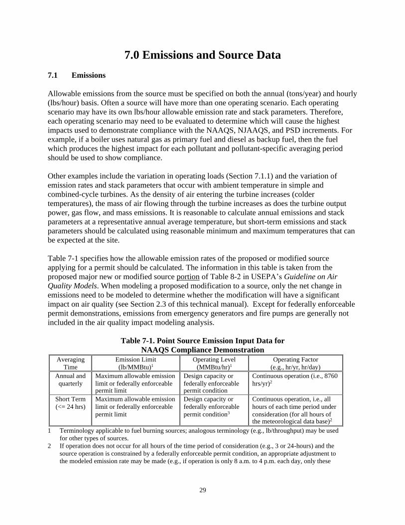
29
7.0 Emissions and Source Data
7.1 Emissions
Allowable emissions from the source must be specified on both the annual (tons/year) and hourly
(lbs/hour) basis. Often a source will have more than one operating scenario. Each operating
scenario may have its own lbs/hour allowable emission rate and stack parameters. Therefore,
each operating scenario may need to be evaluated to determine which will cause the highest
impacts used to demonstrate compliance with the NAAQS, NJAAQS, and PSD increments. For
example, if a boiler uses natural gas as primary fuel and diesel as backup fuel, then the fuel
which produces the highest impact for each pollutant and pollutant-specific averaging period
should be used to show compliance.
Other examples include the variation in operating loads (Section 7.1.1) and the variation of
emission rates and stack parameters that occur with ambient temperature in simple and
combined-cycle turbines. As the density of air entering the turbine increases (colder
temperatures), the mass of air flowing through the turbine increases as does the turbine output
power, gas flow, and mass emissions. It is reasonable to calculate annual emissions and stack
parameters at a representative annual average temperature, but short-term emissions and stack
parameters should be calculated using reasonable minimum and maximum temperatures that can
be expected at the site.
Table 7-1 specifies how the allowable emission rates of the proposed or modified source
applying for a permit should be calculated. The information in this table is taken from the
proposed major new or modified source portion of Table 8-2 in USEPA’s Guideline on Air
Quality Models. When modeling a proposed modification to a source, only the net change in
emissions need to be modeled to determine whether the modification will have a significant
impact on air quality (see Section 2.3 of this technical manual). Except for federally enforceable
permit demonstrations, emissions from emergency generators and fire pumps are generally not
included in the air quality impact modeling analysis.
Table 7-1. Point Source Emission Input Data for
NAAQS Compliance Demonstration
Averaging
Time
Emission Limit
(lb/MMBtu)1
Operating Level
(MMBtu/hr)1
Operating Factor
(e.g., hr/yr, hr/day)
Annual and
quarterly
Maximum allowable emission
limit or federally enforceable permit limit
Design capacity or
federally enforceable permit condition
Continuous operation (i.e., 8760
hrs/yr)2
Short Term
(<= 24 hrs)
Maximum allowable emission
limit or federally enforceable
permit limit
Design capacity or
federally enforceable
permit condition3
Continuous operation, i.e., all
hours of each time period under
consideration (for all hours of the meteorological data base)2
1 Terminology applicable to fuel burning sources; analogous terminology (e.g., lb/throughput) may be used
for other types of sources.
2 If operation does not occur for all hours of the time period of consideration (e.g., 3 or 24-hours) and the
source operation is constrained by a federally enforceable permit condition, an appropriate adjustment to
the modeled emission rate may be made (e.g., if operation is only 8 a.m. to 4 p.m. each day, only these

30
hours will be modeled with emissions from the source. Modeled emissions should not be averaged across
non-operating time periods.
3 Operating levels such as 50% and 75% of capacity should also be modeled to determine the load causing
the highest concentration.
7.1.1 Partial Load and Startup/Shutdown Emissions
The operating scenario analysis may include an evaluation of the various operating loads for an
emission unit or source(s). Because emission rate, exit velocity, and temperature may vary as a
function of operating load or condition, modeling is required to determine which load has the
potential for the highest ambient impact. At a minimum, the emission unit should be modeled
using the design capacity (100% load), or any higher load rates if it can be operated at those
higher rates. Sources that operate for appreciable amounts of time at loads less than the design
capacity require an analysis at partial loads, such as 50% and 75%, to identify the operating
conditions that cause the maximum ground-level concentrations. It should be noted that while
emissions and stack flow rates are relatively linear with load for boilers, emissions and stack
flows for combustion turbines are not linear with load. Engineering data should be submitted by
the applicant to define turbine low load emissions and flow data. In general, load analysis is
required only for larger emission units operating for significant amounts of time at less than
100% load. Applicants should describe their proposed partial-load approach and assumptions in
the modeling protocol. If an operating load is evaluated as worst-case in the air dispersion
demonstration, it must be included as an operating scenario in the permit requirements
A modeling analysis of short-term air quality impact during source startup/shutdown is required
when the applicant details special emission limits during these time periods. Startup/shutdown
modeling may also be requested if these conditions coincide with a very low stack exit velocity
or temperature.
7.1.2 Fugitive Emissions
Fugitive emissions from a facility are those emissions that are not captured and released through
a stack or active vent. A proposed source must model the impact of its fugitive emissions unless
the release height, emission rate, or distance to the property line is such that minimal air quality
impacts would result. A few examples of fugitive emission sources are coal piles, paved and
unpaved roads, and gaseous emissions from landfills. Fugitive emissions are usually modeled as
area or volume sources. All fugitive emission calculations and modeling assumptions should be
discussed in detail and referenced in the modeling protocol.
7.2 Types of Emission Sources
7.2.1 Point Sources
Point sources include emission units that exhaust through stacks, chimneys, exhaust fans,
or vents. The required input data include emission rate, stack height, stack inside diameter, stack
exit temperature, and stack exit velocity. The base elevation of the stack should be based upon
local topographic data. The stack location in Universal Transverse Mercator (UTM) coordinates

31
must also be provided. If a value of 0.0 is input for the exit temperature, AERMOD will adjust
the exit temperature for each hour to reflect the ambient temperature.
7.2.2 Area Sources
Area sources are identified as sources with low level or ground level releases with minimal
thermal or momentum plume rise, and include material storage piles, lagoons and other low-
lying sources. In AERMOD, individual area sources may be represented as rectangles with
aspect ratios (length/width) of up to 10 to 1. Rectangles may be rotated in a clockwise (positive
angle value) or counterclockwise (negative angle value) direction, relative to a north-south
orientation. The rotation angle and the location of the source are specified relative to the
location of the southwest corner of the source. Irregular shaped sources may be represented by a
series of smaller rectangles, or a polygon. The modeling of area sources is discussed in detail in
Section 3.3.2.3 of the AERMOD User’s Guide.
The emission rate for the area source is expressed as grams per second per meter squared
(g/sec/m2). In addition to the emission rate, release height (h), physical dimensions and
orientation of the area source, the applicant may optionally provide the initial vertical dimension
of the area source plume.
Area sources are not affected by the building downwash algorithms in the models. Additionally,
elevated terrain is not considered when modeling impacts from area sources. AERMOD treats
area sources as if in flat terrain, even if elevated receptors are incorporated.
7.2.3 Volume Sources
Volume sources are sources that have initial dispersion prior to release, such as building roof
vents and conveyor belts. Volume sources can also be used to characterize the mobile emissions
associated with construction activities. The modeling of volume sources is discussed in Section
3.3.2.2 of the AERMOD User’s Guide. The location of the volume source is specified relative to
the location of the center of the source. Volume sources are characterized by volume emission
rate gram per second (g/s), emission release height, initial lateral dimension (σyO), and initial
vertical dimension (σzO). The release height is the height of the center of where most of the
plume is emitted from (i.e., the center of the initial volume).
For buoyant sources, such as engine emissions associated with construction/yard activities,
assume that the volume height equals the plume height under annual average (or period average)
conditions. The initial lateral and vertical dimensions represent one standard deviation of the
plume. Therefore, the initial dimensions can be smaller than the release height.
The initial lateral dimension is calculated differently depending on whether the source is a single
volume source or a line source. The initial vertical dimension is calculated differently depending
on the emission release height and the presence of buildings. USEPA’s suggested procedures for
estimating σyO and σzO are listed in Table 7-2. Like area sources, volume sources are not affected
by the building downwash algorithms in the models.

32
Table 7-2. Suggested Procedures for Estimating σyO and σzO *
Type of Source Procedure for Obtaining Initial Dimension
(a) Initial Lateral Dimensions (σyO)
Single Volume Source σyO = length of side divided by 4.3
Line Source Represented by Adjacent Volume Sources σyO = length of side divided by 2.15
Line Source Represented by Separated Volume Sources σyO = center to center distance divided by 2.15
(b) Initial Vertical Dimensions (σzO)
Surface-Based Source σzO = vertical dimension of source divided by 2.15
Elevated Source on or Adjacent to a Building σzO = building height divided by 2.15
Elevated Source not on or Adjacent to a Building σzO = vertical dimension of source divided by 4.3
* Per Section 3.3.2.2 of User’s Guide for the AMS/EPA Regulatory Model – AERMOD EPA-454/B-03-001,
USEPA, Research Triangle Park, North Carolina, September 2004.
7.2.4 Roadways and Line Sources
Line sources are sources that may be represented as a series of volume or area sources, such as
roads, runways, or conveyor belts. Near ground level sources may be modeled using a series of
area sources. As mentioned earlier, in AERMOD individual area sources may be represented as
rectangles with aspect ratios (length/width) of up to 10 to 1. Line sources with an initial plume
depth, such as a conveyor belt or rail line, may be modeled as a series of volume sources. The
number of line sources required to represent the source, N, is calculated as the length of the line
source divided by its width.
In the case of a long and narrow line source such as a rail line, it may not be practical to divide
the source into N volume sources. It is acceptable to approximate the representation of the line
source by placing a smaller number of volume sources at equal intervals along the line source.
In general, the spacing between individual volume sources should not be greater than twice the
width of the line source. However, a larger spacing can be used if the ratio of the minimum
source-receptor separation and the spacing between individual volume sources is greater than
about 3. The total line source emission rate is divided equally among the individual volumes
used to represent the line source, unless there is a known spatial variation in emissions.
The impact of particulate emissions from vehicle traffic (e.g., road dust), in which an initial wake
behind the vehicle is created, should be characterized using multiple volume or area sources.
The number of volume sources, N, should be calculated as described above. The vertical
dimension of the source used in the calculation of σzO is typically equivalent to the height of the
vehicles generating the emissions, commonly 1.5 to 3.0 meters.
7.2.5 Flares
Unlike enclosed flares, open flares are unique point sources as they do not have a defined stack
exit diameter. For modeling, it is necessary to compute equivalent emission parameters, i.e.
adjusted values of temperature, stack height and “stack” inside diameter. AERMOD does not

33
have a source category for flares, and therefore, needs to have the adjustments made by the
modeler. The approach is as follows:
1. Compute the adjustment to stack height (H in meters) as a function of total heat release Q
(in MMBtu/hr):
Hequivalent = Hactual + 0.944(Q)0.478
[Note: 1) some flares are rated in calories per second and the conversion factor is 14.3
Btu/hr for every cal/s; and 2) the adjustment is to account for flame length and assumes
the flame is tilted 45-degrees from the vertical.]
2. Assume a temperature of 1,273 degrees Kelvin (K);
3. Assume an exit velocity of 20 meters/second; and
4. Assume an effective stack diameter deff of,
deff = 0.1755(Q)0.5 meters.
Equivalent diameter is applicable for both vertical and horizontal flares since it is back calculated
from a buoyancy flux assumption. Buoyancy flux is not a function of flare orientation.
Therefore, the equation can be used for both horizontal and vertical flare orientations.
This method pertains to the “typical” flare, and will be more or less accurate depending on
various parameters of the flare in question, such as heat content and molecular weight of the fuel,
velocity of the uncombusted fuel/air mixture, presence of steam for soot control, etc. This
method may not be applicable to every situation; therefore, the applicant may submit their own
properly documented method to the Department for review and approval. Flares may be
modeled with AERSCREEN or AERMOD in screen mode.

34
8.0 Establish Background Air Quality Concentrations
Background air quality concentrations are an essential part of the total air quality concentrations
to be considered in assessing source impacts. Background air quality includes pollutant
concentrations due to: (1) natural sources; (2) nearby sources that were not included in the
modeling analysis; and (3) distant sources (e.g., long-range transport).
Air monitoring data used in the background determination should be representative of the area of
interest (i.e., it should characterize the existing concentrations expected at locations of predicted
maximum impacts). For short-term standards, the diurnal or seasonal patterns of the air quality
monitoring data may differ significantly from the patterns associated with the modeled
concentrations. When this occurs, it may be appropriate to pair the air quality monitoring data in
a temporal manner that reflects these patterns (e.g., pairing by season and/or hour of day). An
applicant’s determination of the appropriate background concentrations must be consistent with
USEPA modeling guidance and justified in the modeling protocol.
8.1 Sources of Background Air Quality Data
There are generally two ways to obtain background air quality concentrations: through an on-site
air quality monitoring network; or through a monitoring network operated by government
agencies. In most cases, monitoring data collected by either the Department or a neighboring
state is used to establish background concentrations. If monitoring data is obtained from an air
monitoring network other than the Department’s, the data must be shown to meet the
Department’s air monitoring quality assurance requirements for representativeness,
completeness, precision, and accuracy.
When possible, an applicant must select a monitor upwind of the existing sources included in the
modeling to avoid double-counting the impact from these sources. In some instances, such as a
multisource modeling analysis, a different background monitor will need to be used than that
proposed in the single-source modeling analysis. Additional guidance can be obtained from
Appendix W to 40 CFR 51 – Guideline on Air Quality Models.
Modeling protocols must specify the monitors selected as representative of background air
concentrations, justify their selections, and list the pollutant concentrations that will be used in
the analysis. Unless instructed otherwise by the Department and regardless of the anticipated
significance or insignificance of the source, the applicant must include a discussion of
background data in the protocol.
In 2015, the Department maintained over 37 monitoring sites in its continuous and manual
monitoring networks. The continuous monitoring network consists of sites that measure CO,
NOx, O3, SO2, and meteorological data by automated instruments (not all pollutants are measured
at all sites). In addition, the continuous monitoring network has real time PM2.5 (TEOM)
monitors. Nonetheless, the data from the PM2.5 real-time analyzer cannot be used for
comparison to the NAAQS or as background for modeling because it is not a USEPA approved
24-hour manual samplers.

35
Table 8-1. List of Pollutants Monitored at Each Site
Monitoring Site NOx SO2 CO O3 PM2.5 PM10
Ancora State Hospital x
Atlantic City x
Bayonne x x x
Brigantine x x x
Camden Spruce Street x x x x x x
Camden-RRF x
Chester x x x x
Clarksboro / Gibbstown a x x a
Colliers Mills x
Columbia WMA x x x x
East Orange x b x b
Elizabeth x x
Elizabeth Lab x x x x
Elizabeth-Mitchell Building xb
Flemington x
Fort Lee Near Road x x
Fort Lee-Library x
Jersey City-Firehouse x x
Jersey City x x x
Leonia x
Millville x x
Monmouth University x
Morristown-Ambulance Squad x
New Brunswick x c
Newark Firehouse x x x x x
Paterson x
Pennsauken x
Phillipsburg x
Rahway x
Ramapo x
Rider University x
Rutgers University x x
Toms River x
Trenton x
Union City x
Washington Crossing x
a. Gibbstown PM2.5 monitor relocated 7 kilometers east to nearby Clarksboro monitoring site
during 2017. b. Discontinued in 2016.
c. New Brunswick PM2.5 speciation monitor relocated to nearby Rutgers University monitoring
site in 2016.

36
Yearly summaries of air quality data collected by NJDEP are available as Air Quality Reports.
These reports can be accessed easily at the following website: http://www.njaqinow.net/. These
reports also contain information on the address and description of each monitoring site in the
NJDEP ambient air quality monitoring network. Air pollutants monitored at each monitoring
site are listed in Table 8-1. A map showing the locations of the ambient air monitoring sites is
contained in Figure 8-1. Further information can be obtained by calling (609) 292-0138.
Figure 8-1. 2014 New Jersey Air Monitoring Sites

37
8.2 Use of Background Values in the Modeling Analysis
Unless air quality data collected from a source specific network are used, the latest three years of
monitoring data should be used irrespective of the meteorological data period used in the
dispersion modeling. Further refinement of these background air quality values such as those
techniques discussed in Section 8.3 of EPA’s Appendix W to 40 CFR 51 – Guideline on Air
Quality Models will be considered by NJDEP on a case-by-case basis.
8.2.1 Deterministic NAAQS and NJAAQS
All NAAQS and NJAAQS not specifically discussed in Section 8.2.2 are deterministic.
First-Tier
The highest, second-highest short-term concentrations from the selected representative monitor
should be used as the background concentration for the short-term deterministic NAAQS (24
hours or less). For long-term deterministic NAAQS and NJAAQS, the maximum value
monitored over three years should be used as background.
Second-Tier
If an applicant believes a background based on second-high values is too high, a second-tier
technical analysis may be made that demonstrates the first-tier value could not reasonably be
assumed to occur at the same time/place as the modeled design value. In this situation, an
alternative background value may be proposed with justification. The proposal is subject to
NJDEP approval.
8.2.2 Statistical Based NAAQS
8.2.2.1 1-Hour NO2
The 1-hour NO2 standard is based on the 3-year average of the 98th-percentile of the annual
distribution of daily maximum 1-hour concentrations. Use of background monitoring data in a 1- hour NO2 NAAQS demonstration is discussed in detail in the USEPA memo “Additional Clarification Regarding Application of Appendix W Modeling Guidance for the 1-Hour NO2
National Ambient Air Quality Standard” (March 1, 2011).
First-Tier
The first-tier background technique is defined by USEPA as the 98th-percentile of the annual
distribution of daily maximum 1-hour values averaged across three years of data from a
representative monitor. That value would be equivalent to the 8th highest daily 1-hour value over
a 365-day monitoring period. The latest three years of monitoring data should be used
irrespective of the meteorological data period used in the dispersion modeling. Normally, the
Department accepts first-tier 1-hour NO2 background values without further justification.

38
Second-Tier
The second-tier background technique uses a 3-year year average of the 98th-percentile of the
available background concentrations grouped into subsets by the four seasons (quarterly) and/or
the 24 hours-of-day. The various options of defining a second-tier background include:
• 2nd-highest 1-hour value from each of the four seasonal (or quarterly) distributions
should be used to represent the 98th-percentile.
• 3rd-highest 1-hour value for each season and hour-of-day combinations should be used
to represent the 98th-percentile.
• 8th-highest 1-hour value should be used to represent the 98th-percentile for hour-of-day
background when the entire year is used (not seasonal).
• 1st-highest values for more detailed temporal pairing, such as season by hour-of day and
day-of-week or month by hour-of-day.
Because the 1-hour NO2 NAAQS is based on the annual distribution of daily maximum 1-hour
values, the diurnal and seasonal patterns of ambient impacts could play a significant role in
determining the most appropriate method for combining modeled and monitored concentrations.
For example, if the daily maximum 1-hour impacts associated with the project emissions
generally occur under nighttime stable conditions whereas maximum monitored concentrations
occur during daytime convective conditions, pairing modeled and monitored concentrations
based on hour of day should provide a more appropriate estimate of cumulative impacts than the
first-tier method that ignores this diurnal pattern. The applicant’s use of a second-tier analysis in
these situations will be subject to NJDEP approval.
8.2.2.2 1-Hour SO2
The 1-hour SO2 standard is based on the 3-year average of the 99th-percentile of the annual distribution of daily maximum 1-hour concentrations. Use of background monitoring data in a 1-hour SO2 NAAQS demonstration is also discussed on pages 17 - 21 of the USEPA memo
“Additional Clarification Regarding Application of Appendix W Modeling Guidance for the 1- Hour NO2 National Ambient Air Quality Standard” (March 1, 2011).
First-Tier
The “first-tier” background technique is defined by USEPA as the 99th-percentile of the annual
distribution of daily maximum 1-hour values averaged across the three years of data from a
representative monitor. That value would be equivalent to the 4th highest daily 1-hour value over
a 365-day monitoring period. The latest three years of monitoring data should be used
irrespective of the meteorological data period used in the dispersion modeling. Normally, the
Department accepts first-tier 1-hour SO2 background values without further justification.

39
Second-Tier
The “second-tier” background technique is to use a 3-year average of the 99th-percentile of the
available background concentrations grouped into subsets by the four seasons (quarterly) or the
24 hours-of-day. The various options of defining a second-tier of SO2 background include:
• highest 1-hour value from each four seasonal (or quarterly) distributions should be
used to represent the 99th-percentile; or
• 4th-highest 1-hour value should be used to represent the 99th-percentile for hour-of-day
background when the entire year is used (not seasonal).
Unlike NO2, there is no significant atmospheric chemistry involved in the formations of SO2.
Therefore, there may be less variation in the diurnal and seasonal monitored values than that of
the 1-hour NO2. However, an examination of the diurnal and seasonal patterns of peak 1-hour
SO2 modeled impacts may show that they occur at different times during the day and/or year than
peak monitored values. In this case, use of a second-tier background may be appropriate. The
applicant’s use of a second-tier analysis will be subject to Department approval.
8.2.2.3 24-Hour and Annual PM2.5
The 24-hour PM2.5 NAAQS is based on the 3-year average of the 98th-percentile of the annual distribution of 24-hour average concentrations. The annual PM2.5 NAAQS is based on a 3-year
average of annual PM2.5 concentrations. Use of background monitoring data in a PM2.5 NAAQS
demonstration is discussed in detail on pages 56-63 of the USEPA document “Guidance for PM2.5 Permit Modeling” (May 2014), EPA-44-/B-14-001. This document can be found at:
https://www3.epa.gov/ttn/scram/guidance/guide/Guidance_for_PM25_Permit_Modeling.pdf
First-Tier (24-Hour)
The “first-tier” background technique is defined as the 98th-percentile of the annual distribution
of daily maximum 1-hour values averaged across the three years of data from a representative
monitor. The latest three years of monitoring data should be used irrespective of the
meteorological data period used in the dispersion modeling. Normally, the Department accepts
first-tier 24-hour PM2.5 background values without further justification.
Second-Tier (24-Hour)
The second-tier background technique uses a 3-year year average of the 24-hour 98th-percentile
of the available background concentrations grouped into subsets by the four seasons (quarterly).
Seasonally-varying monitored background components are likely to be more important factors
for the 24-hour PM2.5 NAAQS than the annual PM2.5 NAAQS. The methods of defining a
second-tier background include:
• 2nd-highest 24-hour PM2.5 value from each seasonal (or quarterly) distributions should
be used to represent the 98th-percentile when monitoring every day; or
• 3rd-highest 24-hour PM2.5 value from each seasonal (or quarterly) distributions should
be used to represent the 98th-percentile when monitoring one in three days.

40
There can be situations where daily background PM2.5 levels are substantially higher on average
during the summer months as compared to the winter months, or vice-versa. If the modeled 24-
hour PM2.5 impact is greater in the season of lower background values, then use of a second-tier
background may be appropriate. The Department advises applicants to evaluate when model
predictions of 24-hour PM2.5 impacts and PM2.5 background levels peak throughout the year
before embarking on a second-tier modeling analysis. The applicant’s use of a second-tier
analysis will be subject to Department approval.

41
9.0 Receptor Network and Meteorological Data
9.1 Receptor Network
Receptor locations used in refined modeling should be of sufficient density to enable the
identification of the highest concentrations and possible exceedances of an ambient air quality
standard or a PSD increment. The design of a receptor network should emphasize the receptor
resolution and location, not the total number of receptors. The selection of receptor locations
should take into consideration the topography, the climatology, monitor sites, and the results of
the initial screening procedures.
The Department recommends that, at a minimum, receptors should include a Cartesian Grid with
receptors spaced as follows:
• 25 m along the facility fence line (if applicable), or property line in the case of risk
assessment modeling;
• 50 m extending from the property line/fence line to 0.5 km;
• 100 m extending from 0.5 km to 1.5 km;
• 250 m extending from 1.5 km to 3 km; and
• 500 m extending from 3 km to 5 km.
The applicant must ensure that receptors appropriately include all publicly accessible locations
(i.e., ambient air). If concentrations are not decreasing clearly near the edge of the receptor grid,
additional receptors should be added. Fine grids (50 m) should be placed over the area(s) of
maximum concentration to ensure that the true maximum concentration is identified. Tall
buildings with balconies or other elevated open-air locations that could be occupied for extended
periods must also be included in the AAQS analysis. These locations should be modeled as “flag
pole” receptors.
In a multisource modeling analysis, receptors only need to be placed in the SIA. Receptors of
interest are the following:
1. location of the maximum concentration predicted from the multisource modeling analysis
of other nearby major sources;
2. location of maximum impact from the proposed source; and
3. location of the maximum impact of the combined effect of the nearby sources and the
proposed source.
The proper location of receptors when modeling the Brigantine Class I area impact is discussed
in Appendix A.
9.2 Ambient Air
The air quality modeling analysis must be performed in all locations of “ambient air”, which has
been defined by USEPA as “that portion of the atmosphere, external to buildings, to which the
general public has access” (40 CFR 50.1(e)). Public access to the facility’s property must be

42
restricted by a physical barrier such as a fence or river with signage along the riverbank. If no
physical barrier exists, receptors shall be placed both on and off the facility’s property when
conducting an air quality impact analysis for compliance demonstration of a NAAQS, NJAAQS,
or a PSD increment. If a physical barrier exists, receptors shall be placed along and outside of
the physical barrier when conducting an air quality impact analysis for compliance
demonstration of a NAAQS, NJAAQS, or a PSD increment.
As a general policy when conducting modeling for risk assessment, receptors are only placed
along and outside of a facility’s property line regardless of public access. There is an exception
to this policy when there is the potential for short-term health impacts on the facility’s property
and significant public presence may occur (e.g. park or recreation structures located on the
facility’s property).
In situations involving leasing arrangements where a source is located on land leased to them by
another source, applicants should apply the guidance contained in the June 22, 2007 USEPA
memorandum entitled: Interpretation of “Ambient Air” In Situations Involving Leased Land
Under the Regulations for Prevention of Significant Deterioration (PSD).
9.3 Meteorological Data
The protocol should describe and justify the use of all meteorological data that will be used in
the modeling analysis. The representativeness of meteorological data is not only a function of
proximity, but other factors, such as nearby terrain.
Five years of representative National Weather Service (NWS) meteorological data, at least three
complete years of prognostic meteorological data, or at least one year of on-site meteorological
data should be used when estimating concentrations with an air quality model. When using
NWS data for air modeling, the Department prefers consecutive years from the most recent,
readily available 5-year period. The Department has processed meteorological data sets for use
by permit applicants when performing air dispersion modeling analyses. The use of standardized
meteorological data sets eliminates the need for each applicant to undertake the resource-
intensive effort of generating this meteorological data on their own. The most recent 2-minute
Automated Surface Observing System (ASOS) meteorological data have been processed using
EPA’s latest meteorological processors and guidance.
The Department maintains five-year AERMET data sets for eight NWS station locations. The
stations locations are: Atlantic City, NJ. Caldwell, NJ, Mount Holly, NJ. Newark, NJ,
Philadelphia, Pennsylvania, Sussex, NJ, Trenton, NJ, and Wilmington, Delaware. Table 9-1
provides the location in decimal degrees, elevation in meters, anemometer height in meters, and
upper air data pairing for each meteorological station. Note that the Profile Base elevation that
should be input to AERMOD is the base elevation of the station as listed in Table 9-1. These
data sets are available to the general public upon request. The applicant should consult with the
Department for the proper AERMET data to use as input to the AERMOD model. Figure 9-1
shows a small-scale wind rose of the dominant wind direction for each station at its spatial
location relative to New Jersey’s borders.

43
Table 9-1. ASOS Meteorological Stations for Use in New Jersey Air Dispersion
Modeling Analyses
Surface
Station
Latitude
(degrees)
Longitude
(degrees)
Base
Elevation
amsl (m)
Anemometer
Height (m)
Upper Air
Station
Atlantic City 39.4520 74.5670 18.0 7.92 Brookhaven, NY
Caldwell 40.8764 74.2828 53.0 7.92 Brookhaven, NY
Mount Holly 39.9407 74.8407 16.0 10.0 Sterling, VA
Newark 40.6828 74.1693 3.0 10.0 Brookhaven, NY
Philadelphia 39.8733 75.2268 8.5 7.92 Sterling, VA
Sussex 41.1993 74.6260 128.0 10.0 Albany, NY
Trenton 40.2768 74.8156 64.9 7.92 Sterling, VA
Wilmington 39.6744 75.6056 24.4 10.0 Sterling, VA

44
Figure 9-1. Location of ASOS Meteorological Stations Processed for use in Air Dispersion
Modeling Analyses in the State of New Jersey

45
10.0 Health Risk Assessments and Other Special Modeling
Considerations
Some special modeling considerations that may need to be addressed by both PSD and non-PSD
sources include, but are not limited to: modeling for a risk assessment, atmospheric deposition,
cooling tower modeling, coastal fumigation modeling, fugitive emissions, start-up/shutdown
impacts, and modeling of other nearby major sources. This section addresses some of these
special requirements and contains a brief discussion of running averages and block averages and
their relation to NAAQS, NJAAQS, and PSD increments. When applicable, the applicant should
address each of these topics in the protocol details of its modeling analysis.
10.1 Health Risk Assessment
Air toxics are natural or man-made pollutants that, when emitted into the air, may cause an
adverse health effect. The federal 1990 CAA Amendments created a list of air toxics, called
“hazardous air pollutants” or “HAPs”, as well as regulations to limit HAP emissions. The air
toxics list generally excludes “criteria pollutants,” that is, those for which NAAQS or NJAAQS
have been established. The exception to this is lead, which is a criteria pollutant and is also
considered to be an air toxic because of its ability to cause significant adverse health impact at
very low exposures. “Lead compounds” are included in USEPA’s HAP list, as are many specific
VOCs, which fall under the VOC pollutant category, and specific heavy metals, which are
included in the particulate matter criteria pollutant category.
Health risk assessments are required for all source operations that emit air toxics above its
reporting threshold for which the Department has designated an inhalation unit risk factor (URF)
or a reference concentration (RfC). The risk assessment shall also include any air toxic emitted
below the reporting threshold that is included in the permit. The majority of health risk
assessments are conducted using the Department’s screening tools. However, under certain
situations, a refined health risk assessment will be required for either a single source operation,
multiple source operations, or on a facility-wide basis. These refined risk assessments may
require the submittal of an air quality modeling and risk assessment protocol. The atmospheric
dispersion modeling techniques used in a refined health risk assessment should generally follow
the guidance outlined in this document. This section contains additional guidance specific to
performing a refined risk assessment. The Department’s webpage,
http://www.state.nj.us/dep/aqpp/risk.html, contains a listing of air toxics for which the
Department has published URF or RfC and other important information concerning risk
assessment procedures. As with an air quality analysis, an air quality modeling and risk
assessment protocol must be approved by the Department before an applicant submits the health
risk assessment.
In addition to the requirements outlined in this document, an air quality impact analysis that
includes a health risk assessment must also include:

46
1. For each air toxic included on the Department’s URF list: the maximum predicted
long-term (chronic) average concentration and its location, the applicable URF, and the
calculated incremental cancer risk (source impact times the URF); and
2. For each air toxic included on the Department’s RfC list: the maximum predicted
long-term or short-term (acute) average concentration and its location, the RfC, and the
calculated hazard quotient (source impact divided by the RfC).
In a refined risk assessment, chronic health risks should be calculated based on a five-year
average (43,800 hours) concentration. For calculating acute health risks, the maximum air toxic
specific short-term concentration modeled (not highest, second-high) should be used.
For chronic health risks, the emission rate modeled should be based on the air toxic tons per year
emission rate listed in the permit application. For air toxics with acute health effects, the
maximum pound per hour emission rate listed in the permit must be used. The use of annualized
hourly emissions to evaluate acute health effects should only be used in the case of fugitive
emissions or tank emissions.
If the air quality modeling protocol is only evaluating air toxic emissions, under certain
situations, the use of the AERMOD non-default control option (FLAT) may be appropriate. This
option ignores receptor elevations and stack-base elevation and assumes flat terrain. This option
will be approved on a case-by-case determination.
In addition to providing incremental cancer risk and hazard quotients at the point of maximum
impact, health risks at the sensitive receptor with the greatest predicted impact also need to be
provided. For health risk assessments, sensitive receptors can include, but are not limited to:
residents of occupied homes, hospitals, schools, and parks. Generally, cancer risks and hazard
quotients need only be calculated at and beyond the applicant’s property line. However, if the
general public has access to the property, the Department may require estimates of the short-term
hazard quotient be made for facility on-site receptors.
The predicted cancer risk and hazard quotient will be compared to the Department’s Risk
Guidelines for Air Toxics listed in Table 10-1 below. The type of action the applicant may need
to take when this guideline value is exceeded will depend on the location, frequency, and
magnitude of the exceedances. For more information on the Department’s Risk Guidelines for
Air Toxics and the Risk Management Committee, consult Technical Manual 1003 “Guidance on
Preparing a Risk Assessment for Air Contaminant Emissions.”

47
Table 10-1. Risk Guidelines for Air Toxics
Cancer Risk Guidelines for Individual Sources
Risk ≤ 1 in a million (1x10⁻⁶) Negligible risk
1 in a million < Risk < 100 in a million Case-by-case review by Risk Management Committee
Risk > 100 in a million (1x10⁻⁴) Unacceptable risk
Facility-Wide Cancer Risk Guidelines
Risk ≤ 10 in a million (1x10⁻⁵) Negligible risk
10 in a million < Risk < 1000 in a million Case-by-case review by Risk Management Committee
Risk ≥ 1000 in a million (1x10⁻³) Unacceptable risk
Non-cancer Risk Guidelines for All Sources
Hazard Quotient ≤ 1 Negligible risk
Hazard Quotient > 1 Case-by-case review by Risk Management Committee
10.2 Cooling Towers
In the permitting of facilities with wet or wet/dry cooling towers, the Department may require
modeling of the cooling tower plumes to determine their potential for causing fogging and icing
of nearby highways. In addition, the cooling towers must be included in the air quality modeling
when their PM10 emissions exceed 1 lb/hr. Details on how the particulate emission rate is
calculated and what assumptions are made must be included in the modeling protocol and
analysis. Cooling towers are normally modeled as a series of point sources, with each cell in the
cooling tower associated with a diameter, exit temperature, and exit velocity. Often, cooling
towers are subject to downwash effects from the cooling tower structure itself. The PM10 and
PM2.5 concentrations due to cooling tower emissions should be added to those caused by other
sources at the facility.
10.3 Coastal Fumigation
Fumigation occurs when a plume that was originally emitted into a stable layer is mixed rapidly
to ground-level when unstable air below the plume reaches plume level. The well-mixed,
unstable air, which develops as air coming from the ocean is heated over land, is known as the
thermal internal boundary layer (TIBL). Sources with tall stacks that are in an area designated as
rural and within 3 km of a large body of water must address coastal fumigation in their modeling
analysis. Other sources located beyond 3 km may also need to examine their coastal fumigation
impacts if the Department believes such an analysis is warranted. Three point source models
capable of simulating coastal fumigation are AERSCREEN, CALPUFF, and the Shoreline
Dispersion Model.

48
10.4 Proximity to Major Sources
In special cases where a proposed source will be near an existing major source, the Department
may require a modeling analysis of emissions from the proposed source along with emissions
from the existing source, even if the predicted impacts of the proposed source are insignificant.
This type of analysis is usually required in response to, or in anticipation of, concerns on the part
of the public and the need to show that the ambient air quality standards will be met in the area
surrounding the proposed source.
10.5 Use of Running Averages and Block Averages
There are two methods of calculating pollutant concentration averages, running averages and
block averages. The time when the block average begins and when it ends is specifically defined
and never varies. For example, all 24-hour averages are calculated from midnight to midnight,
annual averages are calculated from January 1 through December 31, and 3-hour averages are
calculated from midnight (12 p.m.) to 3 a.m., 3 a.m. to 6 a.m., etc. Conversely, running averages
(sometimes called moving averages) have no set time when they must begin and end. A 24-hour
average can begin at 3 a.m. one day and run to 3 a.m. the next day. Running annual averages can
occur over any consecutive 12-month period (e.g. April 1 through March 31, October 1 through
September 30).
As mentioned in Section 3.1.2, New Jersey’s 3-hour, 8-hour, and 24-hour ambient air quality
standards are defined in terms of running hourly averages, and its 3-month and 12-month
ambient air quality standards are defined in terms of running monthly averages. However, all
NAAQS, PSD increments, and the ambient air quality standards of all states surrounding New
Jersey are defined in terms of block averages. It should be noted that New Jersey has no AAQS
for PM10 or PM2.5.
To help avoid confusion in the execution and presentation of the modeling results, the
Department recommends the following:
Initially, calculate all short-term impacts in terms of block averages. Quarterly and
annual concentrations can also be determined as block averages. These values should be
used to determine whether the proposed source has a significant impact. After adding
background and the impact of other sources (if multisource modeling was conducted), if
the total concentration is greater than 90% of the NJAAQS, then running averages should
be calculated.
10.6 Nitrogen Oxide to Nitrogen Dioxide Conversion
Approximately 90% of NOx emissions from a combustion source are emitted in the form of
nitrogen oxide (NO). The rate at which NO will convert to NO2 in the atmosphere will be a
function of the background levels of ozone and other oxidizing agents.
Compliance demonstrations with NO2 annual average NAAQS and NJAAQS, the 1-hour NO2
NAAQS, and the NO2 PSD increment in near-field modeling (source-to-receptor distances less
49
than about 50 km) can be done following the tiers described in Section 4.2.3.4 of USEPA’s
Revised Guideline on Air Quality Models.
Tier 1 - Assume 100% conversion of NOx emissions to NO2.
(assume NO2 emission rate = NOx emission rate)
Tier 2 - The Ambient Ratio Method 2 (ARM2) is based on an empirically derived equation from hourly NO2 and NOx concentrations measured at 580 monitors across the country for more than
10 years. ARM2 uses the ratio provided by the equation to convert AERMOD’s modeled NOx
concentrations to NO2 concentrations. The specific ratio applied will be a function of the
modeled NOx concentration. For example, as the predicted NOx concentration increases, the
ARM2 NO2/NOx ratio may decrease.
The default minimum and maximum NO2/NOx ratios are set at 50% and 90%, respectively. The
minimum NO2/NOx ratio is representative of the modeled source’s in-stack NO2/NOx ratio. An
alternative NO2/NOx value may be applied based on the source’s in-stack emissions ratios, with
the minimum value reflecting the source’s in-stack NO2/NOx ratio. Consultation with the
Department is required for the use of an alternate ARM2 factor. Adequate demonstration of a
source’s in-stack ratio (ISR) is required, and the submission of stack test data to USEPA’s ISR database may be required as part of the documentation process.
The factors to consider on whether ARM2 should be used are listed below. There are no
absolute guidelines regarding these factors. Each factor may be cited in a weight of evidence
evaluation.
1. The specific ratio applied will be function of the modeled NOx concentration; as the
predicted NOx concentration increases, the ARM2 NO2/NOx ratio may decrease. 2. ARM2 will tend to be conservative if there is a short travel time from the stack to the
location of maximum modeled NOx impacts. 3. ARM2 will tend to be conservative if the maximum 1-hour NOx impacts are predicted to
occur at night during winter months, when background ozone is generally low. The
Department can provide maximum hourly concentrations for different monitoring
stations throughout New Jersey. 4. The use of ARM2 is likely conservative if background NO2 is generally low (11 to 16
µg/m3) and the primary source has a Tier 1 modeled NOx impact of less than 380 µg/m3 (200 ppb).
5. If the NO2/NOx ISR for the source is less than 0.5, then ARM2 will tend to be
conservative in predicting NO2 impacts. 6. If the ISR is higher than 0.5, ARM2 may still possibly be used if the minimum ambient
NO2/NOx ratio input is above the 0.5 default minimum value. 7. In areas with high background ozone, use of ARM2 is likely conservative if the primary
source has a Tier 1 modeled NOx impact of less than 282 µg/m3 (150 ppb). 8. In areas with low background ozone, use of ARM2 is likely conservative if the primary
source has a Tier 1 modeled NOx impact of less than 376 µg/m3 (200 ppb).
9. Sensitivity tests suggest ARM2 may underestimate actual NO2/NOx ratios when hourly
ozone concentrations are greater than 80-90 ppb. The September 30, 2014 USEPA

50
clarification memo recommends caution when applying ARM2 if there are more than 7
days with hourly ozone above 80-90 ppb.
Tier 3 - This tier involves using the Ozone Limiting Method (OLM) or the Plume Volume
Molar Ratio Method (PVMRM) algorithms in AERMOD. Consultation with the USEPA
Regional Office is required for this level of evaluation.
As with Tier 2, the default minimum and maximum NO2/NOx ratios are set at 50% and 90%,
respectively. With sufficient supporting data, an alternative minimum NO2/NOx ratio may be
proposed based on the source’s, or a similar source’s measured ISR. When conducting a
multisource modeling analysis, the NO2/NOx ISR recommended for distant sources is 0.2.
Some factors to consider when applying a Tier 3 methodology are listed below.
1. Both PVMRM and OLM require the use of hourly ozone data. Ozone monitoring
locations in New Jersey are listed in Table 8-1.
2. Normally, only one ozone background monitor is used, however, AERMOD includes the
option to specify multiple background files based on geographic relation to the source
and modeling domain.
3. OLM works best for large groups of sources, area sources, and near-surface releases. For
most cases, the OLMGROUP ALL option is recommended.
4. PVMRM works best for relatively isolated and elevated point sources.
The Department recommends 100% NO to NO2 conversion for long-range transport modeling
(e.g., source-to-receptor distances greater than about 50 km).
10.7 Treatment of Horizontal Stacks and Rain Caps
For horizontal stacks or rain caps present on a point source stack, the vertical momentum
component of the exit velocity is effectively removed. Consequentially, a unique approach may
be needed to characterize these stacks. The approach varies by model, as discussed below.
AERMOD: For capped and horizontal stacks that are NOT subject to building downwash
influences, a simple screening approach (Model Clearinghouse Memo from J. Tikvart to K. Eng,
dated 7/9/93) can be applied. This approach uses an effective stack diameter to maintain the
flow rate, and hence the buoyancy, of the plume, while suppressing plume momentum by setting
the exit velocity to 0.01 m/s. To appropriately account for stack-tip downwash, the user should
first apply the non-default option of no stack-tip downwash (i.e., NOSTD keyword). Then, for
capped stacks, the stack release height should be reduced by three actual stack diameters to
account for the maximum stack-tip downwash adjustment while no adjustment to release height
should be made for horizontal releases.
Capped and horizontal stacks that are subject to building downwash should not be modeled using
an effective stack diameter to simulate the lack of vertical momentum. The problem is that the
PRIME algorithms use the stack diameter to define the initial plume radius which, in turn, is
used to solve conservation laws. The user should input the actual stack diameter and exit

51
temperature but set the exit velocity to a nominally low value, such as 0.01 m/s. This approach
will have the desired effect of restricting the vertical flow while avoiding the mass conservation
problem inherent with the effective diameter approach. The approach suggested here will most
likely result in a lower plume height, and therefore, will provide a conservative estimate of
impacts. Also, since PRIME does not explicitly consider stack-tip downwash, no adjustments to
stack height should be made.
The latest version of AERMOD has incorporated the above adjustments for horizontal discharge
and rain cap stacks as a Beta option to the model inputs.

52
11.0 Air Quality Modeling Results
Results of the air quality dispersion modeling analysis are discussed in this section.
11.1 Modeling Submitted in Support of a New Jersey Air Permit Application
Air quality dispersion modeling for the proposals made by a facility must clearly show that
emissions of criteria pollutants will not cause or significantly contribute to an exceedance of any
NAAQS or NJAAQS, and emissions of air toxics will not cause an unacceptable health risk. The
modeling results section of the analysis must contain the following essential information:
1. The location and magnitude of maximum predicted impacts for each modeled criteria
pollutant and air toxic for each applicable averaging time;
2. A comparison of the maximum predicted impact for criteria pollutants to defined
significant impact levels (Table 4-1) for each criteria pollutant modeled;
3. For any proposed source with a predicted insignificant impact for criteria pollutants, a
comparison of the appropriate predicted impact with monitored background
concentration added to applicable state and federal air quality standards;
4. For any proposed source with a predicted significant impact for criteria pollutants, a
comparison of the total impact (the combination of the proposed source impact, the
impact of other existing nearby major sources, and the monitored background
concentration) to applicable state and federal air quality standards; and
5. The results of any additional analyses performed such as a risk assessment or cooling
tower analysis.
In addition, PSD permit air quality evaluation should include a modeling comparison to PSD
increments. The highest long-term average concentrations and the highest, second-high
short-term average concentrations may be used to determine compliance with NAAQS,
NJAAQS, and PSD Class II increments when five years of off-site or at least one year of on-site
meteorological data are used in the modeling analysis. Guidance on demonstrating compliance
with the PM2.5 and PM10 NAAQS is contained at the following webpage,
http://www.nj.gov/dep/aqpp/permitguide.html, and Section 3.2.1 of this document, respectively.
11.2 PSD Permit Applications
In addition to the demonstration required in Section 11.1 above, for PSD permit applications, the
air quality dispersion modeling analysis must also provide the following additional information:
1. A comparison of the predicted impacts to the PSD Class II increments for each pollutant
for which the proposed source is PSD applicable;

53
2. An analysis of the effect of the proposed source on soil and vegetation in the impacted
area and a growth analysis;
3. For any PSD source within 100 km of the Brigantine Class I area, the Department will
normally require a comparison of the predicted impacts to the PSD Class I increments.
For a proposed source with predicted significant impacts at the Brigantine Class I area,
the modeled impact of other PSD increment consuming sources must be included; and
4. For any PSD source within 300 km from the Brigantine Class I area, the FLM for the
Brigantine Class I area (U.S. Fish and Wildlife Service) will, on a case-by-case basis,
require an evaluation of the proposed project’s impact on the Brigantine’s Air Quality
Related Values (AQRVs). AQRVs include visibility and atmospheric deposition of
sulfur and nitrogen.
11.3 Documentation
Copies of model input and output files should be provided with the modeling submittals. The
Department strongly recommends that modeling protocols and analyses be presented in loose
leaf format in a binder so that additions or revisions can be made easily. If this is not done, both
minor and major revisions will require resubmittal of the entire document.
Applicants are reminded that all impact assessments are public information (except process
information marked confidential as defined in N.J.A.C.7:27-1.11) and that major permit
applications frequently undergo extra examination during public hearing/comment processes.
Acronyms and abbreviations should be defined, tables and figures should be clearly labeled, and
excess technical jargon should be avoided.

54
12.0 References
Auer, Jr., A.H., 1978. Correlation of Land Use and Cover with Meteorological Anomalies.
Journal of Applied Meteorology, Volume 17(5), 636-643.
National Park Service, 2010. Federal Land Managers’ Air Quality Related Values Workgroup
Phase I Report (FLAG), Phase I Report – Revised (2010), NPS/NRPC/NRR – 2010/232.
https://www.nature.nps.gov/air/pubs/pdf/flag/FLAG_2010.pdf
USEPA, 1981. A Screening Procedure for Impacts of Air Pollution Sources on Plants, Soils, and
Animals. EPA-450/2-81-078, U.S. Environmental Protection Agency, Research Triangle Park,
NC.
USEPA, 1985. Guideline for Determination of Good Engineering Practice Stack Height
(Technical Support Document for the Stack Height Regulations), Revised. EPA-450/4-80-023R,
U.S. Environmental Protection Agency, Research Triangle Park, NC.
http://www.epa.gov/ttn/scram/guidance/guide/gep.pdf
USEPA, 1987. Ambient Monitoring Guidelines for PSD. EPA-450/4-87-007, U.S.
Environmental Protection Agency, Research Triangle Park, NC.
USEPA, 1998. Interagency Workgroup on Air Quality Modeling Phase II, U.S. Environmental
Protection Agency, Research Triangle Park, NC.
USEPA, 2000. Federal Land Managers’ Air Quality Related Values Workgroup (FLAG) Phase I
Report. U.S. Environmental Protection Agency, Research Triangle Park, NC.
www.nature.nps.gov/air/Pubs/pdf/flag/FlagFinal.pdf
USEPA, 2004a. User’s Guide to the Building Profile Input Program. EPA-454/R-93-038, U.S.
Environmental Protection Agency, Research Triangle Park, North Carolina, NC.
https://www3.epa.gov/ttn/scram/userg/relat/bpipdup.pdf
USEPA, 2013. AERSURFACE User’s Guide, EPA-454/B-08-001 (Revised 01/16/2013), U.S.
Environmental Protection Agency, Research Triangle Park, NC.
https://www3.epa.gov/ttn/scram/7thconf/aermod/aersurface_userguide.pdf
USEPA, 2016a. User’s Guide for the AERMOD Meteorological Preprocessor (AERMET). EPA-
454/B-16-010, U.S. Environmental Protection Agency, Research Triangle Park, NC.
https://www3.epa.gov/ttn/scram/7thconf/aermod/aermet_userguide.pdf
USEPA, 2016b. User’s Guide for the AMS/EPA Regulatory Model (AERMOD). EPA-454/B-16-
011, U.S. Environmental Protection Agency, Research Triangle Park, NC.
https://www3.epa.gov/ttn/scram/models/aermod/aermod_userguide.pdf

55
USEPA, 2016c. User’s Guide for the AERMOD Terrain Preprocessor (AERMAP). EPA-454/B-
16-012, U.S. Environmental Protection Agency, Research Triangle Park, NC.
https://www3.epa.gov/ttn/scram/models/aermod/aermap/aermap_userguide_v11105.pdf
USEPA, 2017. Guideline on Air Quality Models. 40 CFR Part 51, Appendix W.
http://www.epa.gov/ttn/scram/guidance/guide/appw_17.pdf
USEPA, 2010. Federal Land Managers’ Air Quality Related Values Workgroup (FLAG) Phase I
Report – Revised (2010). U.S. Environmental Protection Agency, Research Triangle Park, NC.
https://www.nature.nps.gov/air/pubs/pdf/flag/FLAG_2010.pdf
USEPA, 2015a. Interagency Workgroup on Air Quality Modeling Phase 3 Summary Report:
Long Range Transport and Air Quality Related Values (EPA-454/P-15-003 July 2015), U.S.
Environmental Protection Agency, Research Triangle Park, NC.
https://www3.epa.gov/ttn/scram/11thmodconf/IWAQM3_LRT_Report-07152015.pdf
USEPA, 2015b. AERMOD Implementation Guide. U.S. Environmental Protection Agency,
Research Triangle Park, NC.
https://www3.epa.gov/ttn/scram/7thconf/aermod/aermod_implmtn_guide_3August2015.pdf
USGS, 1993. Digital Elevation Models Data User’s Guide 5. U.S. Geological Survey, Earth
Science Information Center
https://agdc.usgs.gov/data/usgs/geodata/dem/dugdem.pdf

56
APPENDIX A
Additional Issues for PSD Affected New or Modified Sources
This Appendix provides a brief discussion of the additional issues a Prevention of Significant
Deterioration (PSD) affected source must address. Further details concerning PSD regulations
may be found in the Federal Register (45 FR 52676, August 7, 1980) and in the Code of Federal
Regulations (40 CFR 52.21).
A.1 Pre-application Air Quality Monitoring
For any criteria pollutant that the applicant proposes to emit in significant amounts (see Table 2-
1), continuous ambient monitoring data may be required as part of the air quality analysis. If,
however, either (1) the predicted ambient impact, i.e., the highest modeled concentration for the
applicable averaging time, caused by the proposed significant emissions increase (or significant
net emissions increase), or (2) the existing ambient pollutant concentrations, are less than the
prescribed significant monitoring concentrations (SMC) (see Table A-1), the Department has
discretionary authority to exempt an applicant from this air quality monitoring requirement. The
Department will also exempt a source from pre-application monitoring if it believes air quality in
the area is adequately represented by existing monitors. Information on PSD monitoring can be
found in Ambient Monitoring Guidelines for PSD (EPA-450/4-87-007), 1987.
Table A-1. Significant Monitoring Concentrations
Pollutant Air Quality Concentration and Averaging Time
(µg/m3)
CO 575 (8-hr)
NO2 14 (annual)
SO2 13 (24-hr)
TSP 10 (24-hr)
PM10 10 (24-hr)
PM2.5 0*
Ozone A
Lead 0.1 (3-month)
Asbestos b
Beryllium 0.001 (24-hr)
Mercury 0.25 (24-hr)
Vinyl Chloride 15 (24-hr)
Fluorides 0.25 (24-hr)
Sulfuric acid mist b
Total reduced sulfur (including H2S) b
Reduced sulfur (including H2S) b
Hydrogen sulfide 0.2 (1-hr)

57
A: No significant air quality concentration for ozone monitoring has been established. Instead, applicants
with a net emission increase of 100 tons/yr or more of VOCs or NOx subject to PSD would be required to
perform an ambient impact analysis, including pre-application monitoring data.
b: Acceptable monitoring techniques may not be available at this time. Monitoring requirements for this
pollutant should be discussed with the Bureau.
*On January 22, 2013, the U.S. Court of Appeals for the D.C. Circuit vacated and remanded the
PSD rules regarding Significant Impact Levels (SIL) under 52.21(k)(2) and SMC for fine
particulate matter (PM2.5). With respect to SMC, the Court precluded USEPA from using the
PM2.5 SMC to exempt permit applicants from the requirement to compile preconstruction
monitoring data.
Subsequently, on March 4, 2013, USEPA issued a guidance document “Circuit Court Decision
on PM2.5 Significant Impact Levels and Significant Monitoring Concentration Questions and
Answers.” This document is meant to address issues that have resulted from the January 22,
2013 court decision. On page 2, the USEPA provides the following guidance on the statutory
requirement to compile preconstruction monitoring data:
Accordingly, all applicants requesting a federal PSD permit, including those having already
applied for but have not yet received the permit, should submit ambient PM2.5 monitoring
data in accordance with the Clean Air Act requirements whenever either direct PM2.5 or
any PM2.5 precursor is emitted in a significant amount. In lieu of applicants setting out
PM2.5 monitors to collect ambient data, applicants may submit PM2.5 ambient data collected
from existing monitoring networks when the permitting authority deems such data to be representative of the air quality in the area of concern for the year preceding receipt of the
application.
Although the court’s decision related specifically to PM2.5, the decision can be interpreted to also
preclude the use of SMCs to exempt from monitoring for the other PSD affected pollutants.
Therefore, a waiver to the ambient air monitoring requirement cannot be granted based just on
the SMC.
A.2 Post-construction Air Quality Monitoring
Post-construction monitoring may be required when there are valid reasons, such as (1) when the
NAAQS are threatened, and (2) when there are uncertainties in the databases for modeling.
A.3 PSD Baseline Trigger Date
The PSD increments are the maximum allowable increase in ambient pollutant concentrations
that can occur above the applicable baseline concentrations. The following emission changes
must be used to calculate available increment. Sources that should be included in increment
modeling are those within the SIA and may also include sources up to 50 km beyond the SIA.

58
1. The actual emissions increases (or decreases) after the Major Source Baseline Date that
are associated with construction at a major source. The major source Baseline Dates are
as follows:
SO2 and PM10 - August 6, 1975
NO2 - February 8, 1988 PM2.5 - October 20, 2010
2. The actual emission increases (or decreases) at any stationary source permitted after the
Minor Source Baseline Date (listed below).
3. Allowable emissions from PSD sources (including secondary and fugitive emissions)
which have submitted a PSD application prior to the date of application by the proposed
source. If the source is an existing PSD source and has been in operation for more than
two years, actual emissions may be used.
4. Actual emission increases from general area growth.
5. Changes in emissions due to State Implementation Plan (SIP) revisions.
For short-term averaging periods, the difference between the current maximum actual emissions
and the maximum actual emissions as of the applicable baseline date are modeled. The
maximum actual emissions are the highest occurrence or an upper percentile value for that
averaging period during the previous two years of operation. For the annual averaging period,
the difference between the current average actual emissions and the average actual emissions as
of the applicable baseline date are modeled. In both cases, the average actual emissions are
calculated as the average over the previous two-year period.
Many facilities do not have the necessary records to support the calculation of the change in
actual emissions since the applicable baseline date. Therefore, as a conservative approach,
allowable emissions can be used as a screening techniques. This approach assumes no changes
in emissions after the major source baseline date. As another alternative, the Department
recommends that the first level of the increment analysis be accomplished using the actual
emissions from the previous two years for all emission sources included in the analysis. If this
approach results in predicted concentrations above the applicable PSD increment, then the
difference in actual emissions can be determined for the emission unit(s) contributing to the
exceedances and the model rerun. This approach eliminates the need to calculate the difference
in actual emissions for all increment consuming sources.
If the change in actual emissions included a change in stack parameters, then the stack
parameters and emission rates associated with both the baseline case and the current case are
input into the same model run, with the baseline case modeled as negative emissions and the
current case modeled as positive emissions, each with the appropriate stack parameters.
The Department will assist all PSD applicants with their increment analysis by providing air
quality monitoring data on file, parameters for existing sources located in the State, and
modeling analyses developed in support of SIP revisions, when available. It is the responsibility

59
of the applicant to obtain details on specific permits from Department’s files and to obtain
necessary data from any other state(s) or agency(s).
The Department currently has no policy that limits the amount of short-term or long-term
increment one source can consume. However, to allow for future economic development, permit
applicants are discouraged from proposing emissions increases that will consume most or all the
available PSD increment in an area. Note that increment expansion is allowed only from sources
that existed at the time of the baseline date, and the expansion must be attributed to actual
emissions.
The PSD increment major source baseline date is a fixed date found in the regulation associated
with the specific criteria pollutant. The minor source baseline concentration is the concentration
of a pollutant after the first complete PSD permit application affecting the area was received.
That date is referred to as the PSD “Minor Source Baseline Date.” To demonstrate compliance
with PSD increment levels, the area that will be impacted by the project must first be defined and
then the amount of increment available in that area must be calculated by modeling all sources in
that area permitted after the minor source baseline date. The following PSD minor source
baseline dates have been established in New Jersey:
1. New Jersey Portion of the New York - New Jersey - Connecticut Interstate Air Quality
Control Region (Bergen, Essex, Hudson, Middlesex, Monmouth, Morris, Passaic,
Somerset, and Union Counties)
SO2
PM10
November 3, 1977 November 15, 1978
(Exxon) (GAF)
PM2.5 September 4, 2013 (Attainment status)
2. New Jersey Portion of the Metropolitan Philadelphia Interstate Air Quality Control
Region (Burlington, Camden, Gloucester, Mercer, and Salem Counties)
SO2
PM10
October 6, 1977 July 18, 1979
(Seaview Petroleum) (BF Goodrich)
PM2.5 January 13, 2014 (West Deptford Energy)
3. New Jersey Portion of the Northeast Pennsylvania Upper Delaware Valley Interstate Air
Quality Control Region (Hunterdon, Sussex, and Warren Counties)
SO2 November 21, 1980 (Hoffmann LaRoche) PM10 September 20, 1978 (Hoffmann LaRoche) PM2.5 No trigger date to include minor sources
4. New Jersey Intrastate Air Quality Control Region (Atlantic, Cape May, Cumberland, and
Ocean Counties)
SO2 November 17, 1988 (CNG Lakewood) PM10 November 17, 1988 (CNG Lakewood)

60
PM2.5 April 16, 2014 (Ocean Peaking Power)
The PSD minor source baseline date for NO2 is February 8, 1988 for all areas of New Jersey. It
corresponds to the date on which the increments for NO2 were first proposed in the Federal
Register, Volume 53, Number 25, February 8, 1988. Also note that sources may consume
increment in neighboring states but they cannot trigger the minor source baseline date for
increment analysis in the neighboring state.
A.4 Additional Impact Analysis - Growth
This analysis is an estimate of the projected residential, commercial, and industrial growth that
will occur because of the PSD project and an estimate of the air emissions associated with this
growth. Air contaminant emissions associated with any new growth predicted to result from the
proposed project and the air emissions from the proposed PSD project are modeled together.
The applicable background values are added to the resulting modeled concentrations and the
results compared with the applicable NAAQS and PSD increments.
Often the new residential, commercial, and industrial growth estimated to occur because of the
PSD project is negligible. In this case, further modeling analyses for growth are not necessary.
A.5 Additional Impact Analysis - Soils and Vegetation
The purpose of the soils and vegetation analysis, required by 40 CFR 52.21(o), is to assess the
impact of the project emissions on areas of commercial or recreational value. For some
pollutants and monitoring intervals, the NAAQS or the NJAAQS provide sufficient protection
against damage to vegetation. However, these air quality standards may not adequately protect
many commercially grown crops in New Jersey that are classified as sensitive vegetation.
Therefore, the Department requires additional screening for SO2 at the 3-hour and 12-month
intervals. This screening values are adopted from Table 3.1 of the USEPA document A
Screening Procedure for the Impacts of Air Pollution Sources on Plants, Soils, and Animals
(EPA 450/2-81-078) and are shown in Table A-2. Note that the SO2 averaging times are the
same for the demonstrating compliance with NJAAQS, and therefore will not require additional
modeling.
Table A-2. Soils and Vegetation Screening Values
Pollutant Averaging Period Screening Value (µg/m3)a
SO2 3-hour 786
Annual 18 a. The screening value is based on the sensitive vegetation screening value in the USEPA document 450/2-
81-078. This value should be compared to the maximum average ambient air concentration plus
background for the specified averaging period.
If the emission impact is greater than the screening criteria in Table A-1, the applicant should
follow USEPA guidance in the New Source Review Workshop Manual (USEPA 1990) to assess
potential impacts on vegetation. This includes:

61
a) Create an inventory of soils and vegetation with commercial or recreational value in the
impact area (e.g., crops and parks). This may be available from conservation groups,
state agencies, and universities;
b) Review peer-reviewed scientific literature to determine the concentration level (for
appropriate averaging times) of SO2 that would be harmful to each type of vegetation in
the area of impact; and
c) Discuss the nature of the harm and its spatial extent in the modeling report. This analysis
should evaluate the predicted concentrations associated with the averaging periods
addressed in the applicable vegetation impact studies.
Depending on the potential impacts to vegetation information, the applicant may be asked to
provide an additional analysis that follows the seven-step process outlined in USEPA document
450/2-81-078 for estimating the impact from annual soil deposition and the subsequent uptake of
pollutants by plants and animals.
A.6 Class I Area Impact Analysis
All areas of the United States are classified as Class I, II, or III PSD areas. Class I areas are
generally national parks and wilderness areas; Class II areas allow for moderate growth and
represent most areas of the country; and Class III are designated as areas that intend to foster
extensive industrial development. The classifications and associate increment values are
codified at 40 CFR 51.166 and 40 CFR 52.21.
The entire State of New Jersey is designated as a Class II PSD area except for the Brigantine
Wilderness in the Brigantine Division of the Edwin B. Forsythe National Wildlife Refuge
(formerly the Brigantine National Wildlife Refuge), which is a Class I PSD area.
The USEPA is to be informed of all permit applications related to major stationary source or
major modifications per 40 CFR 51.166(p). If a major stationary source or major source
modification is proposed that results in a predicted impact concentration greater than 1 µg/m3 on
a 24-hour basis within 10 km of a Class I area, then the source is PSD affected for that pollutant.
For a proposed PSD source or modification located within 50 km of the Brigantine Class I area,
the applicant must conduct a modeling analysis of the source’s impact at the Class I area. A
proposed PSD source or modification between 50 and 300 km of this Class I area may be
required to evaluate its Class I area impact on a case-by-case basis. The Federal Land Manager
(FLM) is to be provided written notice of any permit application for any proposed major
stationary source or major modification within 300 km of a Class I Area per 40 CFR 52.21(p).
The FLM normally determines the level of analysis required beyond the items outlined in this
section of the guidance document. The Department may require a Class I increment analysis of
sources closer than 100 km from the Brigantine Class I area even when not required by the FLM.
The basic procedures that should be used in a Class I area analysis can be found in the following
documents:
• Federal Land Managers Air Quality Related Values Workgroup Phase I Report (FLAG,
2000), Federal Land Managers’ Air Quality Related Values Work Group (FLAG) Phase I
Report – Revised (2010) NPS/NRPC/NRR – 2010/232

62
https://www.nature.nps.gov/air/pubs/pdf/flag/FLAG_2010.pdf
• Interagency Workgroup on Air Quality Modeling Phase 3 Summary Report: Long Range
Transport and Air Quality Related Values (EPA-454/P-15-003 July 2015)
https://www3.epa.gov/ttn/scram/11thmodconf/IWAQM3_LRT_Report-07152015.pdf
• Reassessment of the Interagency Workgroup on Air Quality Modeling (IWAQM) Phase 2
Summary Report: Revisions to Phase 2 Recommendations (EPA-454/R-16-007 December
2016), and,
https://www3.epa.gov/ttn/scram/appendix_w/2016/IWAQM_Phase2_Reassessment_2016.pdf
• Technical Support Document (TSD) for AERMOD-Based Assessments of Long-Range
Transport Impacts for Primary Pollutants (EPA-454/B-16-007 December, 2016).
https://www3.epa.gov/ttn/scram/appendix_w/2016/AppW_LRT_TSD.pdf
The FLM's permit review process consists of three main analyses:
• An air quality analysis to ensure that the pollutant levels do not exceed NAAQS and PSD
increments;
• An AQRV analysis to ensure that the Class I area air quality related values are not
adversely affected by the proposed emissions; and
• A Best Available Control Technology (BACT) analysis to ensure that the emission
increases from the proposed facility are minimized using appropriate pollution control
equipment.
The FLM for the Brigantine Class I area is the United States Fish and Wildlife Service (F&WS).
Catherine Collins is currently the F&WS permitting lead on PSD applications affecting the
Brigantine Class I area. Contact information is listed below.
Federal Land Manager
US Fish and Wildlife Service
National Wildlife Refuge System
Branch of Air Quality
7333 West Jefferson Ave., Suite 375
Lakewood, Colorado 80235-2017
(303) 914-3804
[email protected] or [email protected]
Guidance on Class I area modeling issues may be obtained from Tim Allen of the F&WS
(303-914-3802, [email protected]). Contacts from the local F&WS office are: Wendy Walsh
at 609-382-5274, and Alicia Protus at 609-382-5266.
A.6.1 Class I PSD Increments
As discussed in USEPA’s Guideline on Air Quality Models, the type of modeling conducted to
predict PSD increment consumption at the Brigantine Class I area will depend on the location of

63
the source. Those sources located within 50 km will use a steady-state model such as AERMOD
in their modeling analysis. If the source is greater than 50 km from the Class I area, impacts can
be conservatively predicted at an arc of receptors 50 kilometers from the source in the radial
direction of the Brigantine Wilderness Area. Any additional long range transport modeling
should be investigated in consultation with the Department and the USEPA Regional Office.
Table A-3. PSD Class I Significant Impact Levels and PSD Increments
Pollutant
Averaging
Period
Class I Significant Impact
Levels (µg/m3)
Class I PSD Increments (µg/m3)
SO2 3-hr 1.0 25
24-hr 0.2 5
Annual 0.1 2
PM2.5 24-hr 0.27a 2
Annual 0.05a 1
PM10 24-hr 0.3 8
Annual 0.2 4
NO2 Annual 0.1 2.5
a) Revised 24-hour and annual PM2.5 Class I SIL per April 17, 2018 EPA guidance memo..
The Class I significant impact levels, as well as the Class I PSD increments are listed in Table A-
3. For sources modeling PM10, sulfate and nitrate formed during plume transport to the Class I
area should be added to the predicted impact due to direct PM10 emissions. A PSD project
whose proposed impact exceeds the Class I significant impact levels at the Brigantine Class I
area must conduct a multisource modeling analysis to determine cumulative increment
consumption.
A.6.2 Class I Area Air Quality Related Values (AQRVs)
In addition to the PSD increments, there are requirements for the protection of various Class I
area resources that might be affected by air pollution. These "air quality related values", or
"AQRVs", include visibility, vegetation, lakes and streams, soils, fish, and animals. Pursuant to
the CAA, FLMs have an affirmative responsibility to protect AQRVs. Among the Brigantine
Class I area’s AQRVs of interest to the FLM are visibility, the impact of sulfur/nitrogen
deposition on soils and water quality, and ozone damage to sensitive vegetation. The FLM’s
recommendations on how the applicant should assess its impact on Class I areas are found in the
FLAG documents. Below is a brief summary of the AQRV issues.
A.6.2.a Visibility Impairment Analysis
Visibility in important natural areas is protected under several provisions of the CAA. Visibility
impairment is caused by light scattering and light absorption associated with particles and gases
in the atmosphere. In most areas of the country, light scattering by PM2.5 is the most significant
component of visibility impairment. The key components of PM2.5 contributing to visibility
impairment include sulfates, nitrates, organic carbon, elemental carbon, and crustal material. In
1999, USEPA issued revisions to the regulations to address visibility impairment in the form of
regional haze, which is caused by numerous, diverse sources. The Federal Land Managers’ Air

64
Quality Related Values Work Group (FLAG) visibility modeling recommendations are divided
into distinct sections to address requirements for near field plumes compared to a background,
and for long-range transport of plumes and aggregation of plumes that affect a vista.
The visibility impairment analysis should evaluate both the impacts to the immediate area
affected by the source emissions, and the impacts from chemical transformation and long-range
transport of source emissions to nearby Class I areas. Any proposed PSD source or modification
located within 300 km of the Brigantine Class I area, for which the FLM has requested a Class I
evaluation must address its visibility impact at the Class I area. If the source is located within 50
km of the Brigantine Class I area, a method of assessing the source’s visibility impact due to
coherent plumes should be used. Applicants should first model their potential plume impacts
using the USEPA’s screening model, VISCREEN, or, if the next level of analysis is called for,
the USEPA’s PLUVUE II. Both models use steady-state, Gaussian-based plume dispersion
techniques to calculate one-hour concentrations within an elevated plume. These two models
calculate the change in the color difference index (ΔΕ) and contrast between the plume and the
viewing background. Values of ΔΕ and plume contrast are based on the concentrations of PM2.5
(including sulfates), NO2, and the geometry of the observer, target, plume, and the position of the
sun. PLUVUE II also allows consideration of the effects of secondarily formed sulfates.
A.6.2.b Atmospheric Deposition Analysis
Emissions of nitrogen, sulfur, mercury and other secondary pollutants, can, in sensitive
ecosystems, change soil and water characteristics and the biodiversity of the ecosystem. To
address the relationship between deposition and ecosystem effects, the FLMs have developed
estimates of critical loads. A critical load is defined as “A quantitative estimate of an exposure
to one or more pollutants below which significant harmful effects on specified sensitive elements
of the environment do not occur according to present knowledge.”
Deposition of sulfur and nitrogen has the potential to affect terrestrial, freshwater, and estuarine
ecosystems on FLM lands. The FLM has identified, where possible, AQRVs sensitive to
deposition of sulfur and nitrogen on FLM lands and the critical loads associated with those
AQRVs. A proponent of a source of new emissions with the potential to contribute to sulfur or
nitrogen deposition in a FLM area should consult with the FLM to determine what analyses are
needed to assess AQRV effects. The FLM may request a deposition impact analysis as
summarized below.
1. Estimate the current deposition rate to the FLM area. A list of monitoring sites providing
data to characterize deposition in FLM areas is included on the respective agencies
websites.
2. Estimate the future deposition rate by adding the existing rate, the new emissions’
contribution to deposition, the contribution of sources permitted but not yet operating,
and then subtracting the credit for enforceable emissions reductions. Modeling of new,
reduced, and permitted but not yet operating emissions’ contribution to deposition should
be conducted following current USEPA modeling guidance.

65
3. Compare the future deposition rate with the recommended screening criteria (e.g., critical
load, concern threshold, or screening level value) for the affected FLM area.
A.6.3 Class I Required Receptors
When conducting a Class I impact analysis, the impact at 44 pre-selected receptors at the
Brigantine Class I area must be evaluated. A listing of the latitude, longitude, and height above
sea-level of these sensitive receptors can be downloaded at the following webpage:
http://www.nature.nps.gov/air/Maps/Receptors/index.cfm. Figure A-1 shows the location of
these receptors on a map.

66
Figure A-1. Required Receptor Locations in Brigantine Division of the
E.B. Forsythe National Wildlife Refuge

67
APPENDIX B
Example Air Quality Analysis Checklist
This checklist recommends a standardized set of data and a standard basic level of analysis
needed for modeling submittals. The checklist implies a level of detail required to assess
compliance with the PSD increments, the NAAQS, and the NJAAQS. Individual cases may
require more or less information and the reviewing authority should be consulted at an early
stage in the development of a data base for a modeling analysis.
At pre-application meetings between the applicant and the reviewing authority, this checklist
should assist the participants as they work to develop a consensus on the data base, modeling
techniques and overall technical approach prior to the actual analyses. By reaching agreement
on these items prior to submission of the applicant’s modeling, applicants may reduce the
chances of a misunderstanding concerning the final results and the need for additional analyses.
1. Source location map(s) showing location with respect to:
• Urban areas
• PSD Class I areas
• Potential environmental justice areas
• Nonattainment areas
• Topographic features (terrain, lakes, river valleys, etc.)
• Other major existing sources
• State/local/on-site air quality monitoring locations
• Plant layout on a topographic map covering a 1 km radius of the source with
information sufficient to determine GEP stack heights
2. Information on urban/rural characteristics:
• Land use within 3 km of source classified per Auer (1978): Correlation of land use
and cover with meteorological anomalies, J. Appl. Meteor., 17: 636-643
• Population (total and density)
• Based on current guidance determination of whether the area should be addressed
using urban or rural modeling methodology
3. Criteria and hazardous air pollutant emissions and operating/design parameters for
proposed major sources:
• Allowable annual emission rates (tons/yr) and operating rates
• Maximum design load short-term emission rate (lbs/hr)
• Associated emissions/stack characteristics as a function of load for maximum,
average, and minimum operating conditions. Screening analyses may be employed to
determine the constraining load condition (e.g., 50%, 75%, or 100% load) to be relied
upon in the short-term modeling analysis.
- location (UTM’s)
- height of stack (ft or m) and grade level above MSL
- stack exit diameter (ft or m)
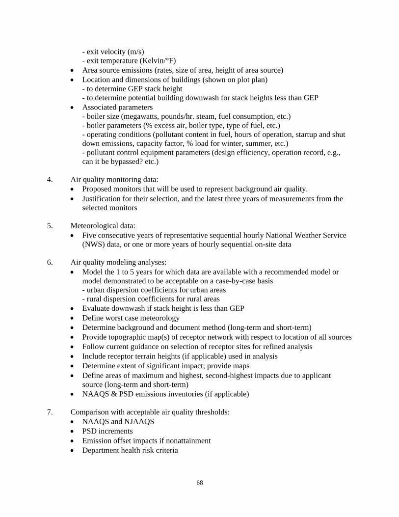
68
- exit velocity (m/s)
- exit temperature (Kelvin/°F)
• Area source emissions (rates, size of area, height of area source)
• Location and dimensions of buildings (shown on plot plan)
- to determine GEP stack height
- to determine potential building downwash for stack heights less than GEP
• Associated parameters
- boiler size (megawatts, pounds/hr. steam, fuel consumption, etc.)
- boiler parameters (% excess air, boiler type, type of fuel, etc.)
- operating conditions (pollutant content in fuel, hours of operation, startup and shut
down emissions, capacity factor, % load for winter, summer, etc.)
- pollutant control equipment parameters (design efficiency, operation record, e.g.,
can it be bypassed? etc.)
4. Air quality monitoring data:
• Proposed monitors that will be used to represent background air quality.
• Justification for their selection, and the latest three years of measurements from the
selected monitors
5. Meteorological data:
• Five consecutive years of representative sequential hourly National Weather Service
(NWS) data, or one or more years of hourly sequential on-site data
6. Air quality modeling analyses:
• Model the 1 to 5 years for which data are available with a recommended model or
model demonstrated to be acceptable on a case-by-case basis
- urban dispersion coefficients for urban areas
- rural dispersion coefficients for rural areas
• Evaluate downwash if stack height is less than GEP
• Define worst case meteorology
• Determine background and document method (long-term and short-term)
• Provide topographic map(s) of receptor network with respect to location of all sources
• Follow current guidance on selection of receptor sites for refined analysis
• Include receptor terrain heights (if applicable) used in analysis
• Determine extent of significant impact; provide maps
• Define areas of maximum and highest, second-highest impacts due to applicant
source (long-term and short-term)
• NAAQS & PSD emissions inventories (if applicable)
7. Comparison with acceptable air quality thresholds:
• NAAQS and NJAAQS
• PSD increments
• Emission offset impacts if nonattainment
• Department health risk criteria

69
APPENDIX C
Odor Modeling Procedures
C.1 Odor Modeling Procedures
The mechanisms of odorant dispersion in the atmosphere are the same as the dispersion of other
pollutants. However, there are some special issues that must be considered when attempting to
quantify a source’s odor impact with dispersion modeling. Among them are determining the
emission rates of the odor-producing pollutants (odorants), the high degree of subjectivity in the
perception and intensity of odors, the short time period over which odors are observed, and the
enhancing or masking of odors by the combinations of odorants. In addition, there are no
dispersion models or modeling techniques recommended by the USEPA for odor modeling.
N.J.A.C. 7:27-5 (Prohibition of Air Pollutants) states that a source shall not emit air
contaminants in such quantities and duration as to unreasonably interfere with the enjoyment of
life or property. Therefore, the Department does on occasion need to evaluate or review
modeling of new or modified sources capable of causing odor problems. In addition, odor
modeling may be required of a new, reconstructed, or modified municipal wastewater/sludge
handling or treatment facility. Although there is no USEPA guidance on the issue, there have
been several scientific studies and technical papers written about odor modeling. The
Department has reviewed the available literature and has developed guidance for assessing a
source’s odor impact with dispersion modeling. Predictions made in an odor modeling analysis
following this guidance would only be considered an indication of the future odor impact of the
source, not the definitive answer. It should be considered a tool in setting either a dilution-to-
threshold (D/T) odor emission limit or pound per hour pollutant specific emission rate for the
source.
C.2 Odor Modeling Techniques
The Department currently recommends two methods to model odor impact. The method selected
will be a function of the number of odor-producing pollutants emitted from the source.
Regardless of the method used, the analysis must provide predictions of maximum odor impact
at sensitive receptors near the source. Sensitive receptors include, but are not limited to,
residents of occupied homes and residential areas, employees and customers at industrial,
commercial, or government establishments, schools, hospitals, and visitors at a recreational
public place such as park or playground. Submittal of predicted odor frequency tables also
provides useful information in the review of a source’s odor impacts. As with other air quality
impact analyses, the Department requires that a protocol be submitted and approved before the
odor modeling analysis is conducted.

70
C.3 Sources that Emit One Primary Odor Producing Pollutant
In this situation, the interaction of pollutants masking or enhancing a perceived odor should be
minimal. Therefore, the odor producing pollutant can be modeled by entering the pollutant’s
emission rate in grams per second into the selected model. The model’s predicted concentration
(in mass per volume, µg/m3) can then be compared to the pollutant’s specific odor threshold.
C.4 Sources that Emit Several Odor Producing Pollutants
When there are numerous pollutants being emitted from a source, there is a much higher
potential for interactions where various odorants may mask or enhance a perceived odor.
Therefore, a dilution to threshold (D/T) approach to quantifying odors should be used in the
analysis. D/T is dimensionless and is a measure of how many volumes of odor-free air must be
added to a sample of contaminated air in order to reduce its odor level below the detection level.
The odor emission rate of the source is expressed as the product of the D/T in air directly emitted
by the source and the volume flow rate. To obtain the correct magnitude of D/T, the model
selected should be set to predict g/m3, not µg/m3.
In the measurement of a source’s D/T emission rate, the odorous air sample from the source is
diluted with equal volumes of odor-free air until an odor is no longer perceptible. For example,
an odorous air sample that was diluted with 100 volumes of odor-free air to reach the 50% odor
perceptibility would have an odor level of 100 D/T.
C.5 Conversion of 1-Hour Modeled Concentrations to Short-term Averages
An odor modeling analysis can be conducted with either a puff (fluctuating plume) model or one
of the standard Gaussian models recommended by the USEPA such as the AERMOD model. If
a puff type model such as TRC’s Odor Model or USEPA’s INPUFF model is used, no
conversion is necessary because short-term D/T values or pollutant concentrations will be
predicted by the model. However, if a model such as AERMOD is used, the predicted one-hour
D/T or pollutant concentration needs to be converted to short-term peak value of 5 minutes or
less.
Review of the available literature indicates the relationship between a 1-hour concentration and a
short-term peak concentration such as a five-minute average is a function of meteorology
(principally atmospheric stability), the release height of emissions, the distance from the source
to receptor, building downwash, and surface roughness. In the paper A Conversion Scheme for
ISC Model In Odor Modeling (Samuel S. Cha, Zhenjia Li, and Karen E. Brown, 1992. AQMA
85th Meeting, 92-153.02), a technique was developed for converting 1-hour concentrations to
5-second concentrations for point sources. Conclusions reached in the paper indicate that the
peak/mean ratios depend on the meteorological condition, the type of source and the receptor
location. A summary of their results for point sources with a 20-meter plume height and a 40-
meter plume height is given in Table C-1. The paper Odor Modeling - Why and How (Duffee,
R.A., M. A. O’Brien, and M. Ostojic, 1989. AWMA Specialty Conference) compares 1-hour
ISCST predictions to the instantaneous predictions of the INPUFF model. When modeling an

71
m p
area source during stable conditions, a relatively constant conversion ratio of approximately 7
was found at receptor distances of 0.8 km, 1.6 km, and 2.4 km.
Table C-1. Conversion Factors for Peak-To-Mean Ratio
Distance (m)
B Stability:
Wind Speed: 2 m/s (4.5 mi/hr)
D Stability:
Wind Speed: 6 m/s (13.4 mi/hr)
E Stability:
Wind Speed: 2 m/s (4.5 mi/hr)
Case I: Point Source Plume Height = 40 Meters
100 45.0 6.0 8.3
200 38.5 7.3 8.3
300 23.2 8.5 10.1
400 16.1 10.2 10.9
600 12.8 12.4 12.7
800 12.6 13.3 13.1
1,000 (0.62 mi) 12.4 10.2 15.6
Case II: Point Source Plume Height = 20 Meters
100 36.0 6.0 5.6
200 14.7 9.7 7.8
300 11.6 12.6 10.9
400 11.0 10.3 12.6
600 10.8 7.4 10.9
800 10.6 6.7 8.4
1,000 (0.62 mi) 10.4 6.6 7.3
Though often too simplistic, another method of converting values to shorter averaging times is
the power law relationship. The following is an example of using the power law to convert a
1-hour concentration or D/T value to a five-minute average:
Cp = Cm (t /t )0.2
where: Cp = 5-minute average concentration or D/T
Cm = 1-hour average concentration or D/T
tp = 5 minutes
tm = 60 minutes
An applicant planning to conduct odor modeling with a model similar to ISC3 or AERMOD can
suggest the use of a conversion ratio based on the above discussion or propose their own. The
Department will review the proposed conversion ratios in the modeling protocol before they are
approved for use in the analysis.
C.6 Odor Modeling Results
Once short-term pollutant concentrations are calculated, they must be compared to odor
detection and complaint levels. Odor detectability, or the odor threshold, is usually defined as
the point at which 50% of a given population will perceive an odor. Table C-2 lists some of the

72
published odor detection levels of pollutants that often cause odor problems. Odor complaint
levels are usually 2 to 3 times higher than the odor threshold levels. The Connecticut
Department of Environmental Protection odor limits given in Table C-2 are considered nuisance
levels. Applicable odor detection and complaint levels for odor producing emissions from a
proposed source should be discussed in the modeling protocol.
Based on the results of the modeling, a D/T emission limit at the source is set which ensures
offsite D/T values will be at an acceptable level. Odor-causing compound(s) from a new,
reconstructed, or modified source should have an odor intensity of less than 5 D/T at the
sensitive receptor with the highest impact. Once the D/T emission limit is set for a facility, it
can later be verified by source testing when the facility is built.
Table C-2. Published Odor Thresholds
Odorant Odor Thresholda
(µg/m3)
Odor Limitb
(µg/m3)
Odor Thresholdc
(µg/m3)
Odor Detectiond
(µg/m3)
Acetaldehyde 120 --- 90 90
Ammonia --- --- 3,615 3,700
Carbon Disulfide --- --- 342 3,900
Dimethyl Disulfide --- --- --- 66
Dimethyl Sulfide --- --- --- 51
Hydrogen Sulfide --- 6.3 11.3 5.5
Methyl Mercaptan --- 2.2 3.4 2.4
Phenol 230 461 153 500
Styrene 640 638 1,360 1,300
Trimethyl Amine --- --- 1.1 6
a. Geometric mean of all odor threshold detection levels in literature reviewed by authors, values from
Reference Guide to Odor Thresholds for HAPS Listed in the Clean Air Act Amendments of 1990 (Draft),
1991, TRC Environmental Consultants.
b. Connecticut DEP - 15-minute average of concentration considered a nuisance.
c. Geometric mean of all odor threshold detection levels in literature reviewed by authors: “Odor as an Aid
to Chemical Safety: Odor Thresholds Compared with TLV and Volatilities for 214 Industrial Chemicals in
Air and Water Dilution” from Journal of Applied Toxicology Vol. 3 No. 6, 1983.
d. Represents the 50% detection level: “The Odor Impact Model” from Journal of Air and Waste
Management Vol. 41 No. 10, October 1991.
C.7 Odor Testing
I. Introduction
The purpose of this document is to provide guidance in the use of odor panel testing to determine
dilutions-to-threshold (D/T) levels. This document should not be considered as a substitute for a complete
testing protocol, which must be source specific. All sampling and analysis shall be performed in
accordance with the approved protocol. Unapproved deviation from the protocol is not acceptable and
will be justification to require repetition of the test project.
II. Test Method

73
The D/T will be determined at the source emission point using ASTM Method E679-91, Standard Practice
for Determination of Odor and Taste Thresholds By a Forced-Choice Ascending Concentration Series
Method of Limits.
III. Sampling
1. Samples should be collected into tedlar bags using a sampling line made of an odor-free, chemically
inert and non-reactive material, such as teflon. If sulfur compounds are suspected to be present, the tedlar
bag should not have a stainless steel valve. The sampling train must allow for the transfer of the gas
through the sample line directly into the bag without going through any sources of potential
contamination, such as pumps or rotometers. The evacuated container sampling procedure listed in EPA
Reference Method 18, Section 7.1.1, is recommended. Alternatives must be approved by the
Department’s Emission Measurement Section, which can be contacted at 609-984-3443.
2. A new tedlar bag is required for each sample. Bags should be pre-purged with carbon filtered air for
48 hours to remove background odors prior to being used for sampling. New sampling line tubing should
be used for each sample and the line should be as short as practical.
3. The sample line and bag should be pre-conditioned by filling the bag with the odorous sample and then
emptying the bag.
4. The sampling location must be approved by the Department’s Emission Measurement Section.
5. Sampling should be 5-minute grab samples, unless otherwise approved. The number of samples
required will be determined in the source specific protocol. In general, sampling will be required under
worst case operating conditions. At least one sample will be a duplicate, where the two evacuated
containers used to fill the tedlar bags will be manifolded by a tee fitting to a common pump. The goal for
the duplicate sample is agreement within +20% of the original, analyzed by the same odor panel on the
same day. One field blank sample of odor free air should be collected for each day of sampling.
6. The tester is responsible for collecting a sufficient volume; however, in general, a 10-liter sample
should be sufficient.
7. Once collected, samples should be maintained at ambient temperatures and protected from direct
contact with the sun. If condensed moisture is expected in the sample bags under these conditions, the
tester must address this issue, either through pre-dilution with odor-free air so that there is no visible
moisture, or by other approved means. If pre-dilution is utilized, the results will have to be adjusted by
the dilution factor.
IV. Analysis
1. Analysis will be done with an odor panel by means of a forced choice triangular dynamic dilution
olfactometer. The odor panel should consist of a minimum of 8 panelists. The greater the number of
panelists, the greater the accuracy of the odor determination. Panelists should be trained and screened for
their ability to smell the odors of interest. Individuals with normal sensitivity should be selected as
panelists.
2. Samples should be analyzed within 8 hours of sample collection when possible; however, sample

74
holding time may not exceed 24 hours under any situation.
3. The olfactometer should be constructed of odor-free materials. In addition, parts that come into direct
contact with the sample must also be chemically inert and non-reactive and must also have the ability to
be purged or cleaned quickly to make them odor-free in case of contamination. The sample should be
directly interfaced with the olfactometer, with the connection being as short as possible and made of the
same materials listed above.
4. The dilution air, olfactometer-to-subject interface and presentation method should be as described in
the Guidelines for Odor Sampling and Measurement by Dynamic Dilution Olfactometry document
(revised Draft May 1993) of the AWMA EE-6 Subcommittee on the Standardization of Odor
Measurement. Air flow per sniff port should be established at 8 liters per minute (lpm), with a minimum
acceptable flow rate of 6 lpm.


