TBEST Model Enhancements - Parcel Level …...TBEST Model Enhancements—Parcel Level Demographic...

TBEST Model Enhancements - Parcel Level Demographic

Data Capabilities and

Exploration of Enhanced Trip Attraction Capabilities

September 2011

Final Report

Contract Number BDK85 977-05

ii

DISCLAIMER The contents of this report reflect the views of the authors, who are responsible for the facts and the accuracy of the information presented herein. This document is disseminated under the sponsorship of the Department of Transportation University Transportation Centers Program and the Florida Department of Transportation, in the interest of information exchange. The U.S. Government and the Florida Department of Transportation assume no liability for the contents or use thereof.

iii

TBEST Model Enhancements Parcel Level Demographic

Data Capabilities and

Exploration of Enhanced Trip Attraction Capabilities

Final Report

Prepared for

State of Florida Department of Transportation

Public Transit Office 605 Suwannee Street, MS 30

Tallahassee, Florida 32399-0450

C/O Project Managers: Daniel Harris and Amy Datz

Prepared by

Steven Polzin, Xuehao Chu, Rodney Bunner, Abdul Pinjari, Martin Catala

National Center for Transit Research Center for Urban Transportation Research (CUTR)

University of South Florida 4202 East Fowler Avenue, CUT100

Tampa, Florida 33620-5375

September 2011

Contract Number BDK85 977-05

v

HNICAL REPORT STANDARD TITLE PAGE

1. Report No.

2. Government Accession No.

3. Recipient's Catalog No.

4. Title and Subtitle

TBEST Model Enhancements—Parcel Level Demographic Data Capabilities and Exploration of Enhanced Trip Attraction Capabilities

5. Report Date

September 2011

6. Performing Organization Code

7. Author(s)

Steven Polzin, Xuehao Chu, Rodney Bunner, Abdul Pinjari, Martin Catala

8. Performing Organization Report No.

9. Performing Organization Name and Address

National Center for Transit Research, Center for Urban Transportation Research University of South Florida 4202 East Fowler Avenue, CUT100, Tampa, FL 33620-5375

10. Work Unit No. (TRAIS)

11. Contract or Grant No.

FDOT BDK85 977-05, DTRT07-G-0059.

12. Sponsoring Agency Name and Address

State of Florida Department of Transportation Public Transit Office 605 Suwannee Street, MS 30 Tallahassee, Florida 32399-0450

Research and Innovative Technology Administration U.S. Department of Transportation Mail Code RDT-30 1200 New Jersey Ave, SE, Room E33 Washington, D.C. 20590-0001

13. Type of Report and Period Covered

Final Report, September 2011

14. Sponsoring Agency Code

15. Supplementary Notes

16. Abstract

FDOT, in pursuit of its role to assist in providing public transportation services in Florida, has made a substantial research investment in a travel demand forecasting tool for public transportation known as Transit Boardings Estimation and Simulation Tool (TBEST). TBEST incorporates supporting databases that allow users to model transit services for purposes of determining future needs and optimizing current resource deployments by targeting the best markets and route configurations. This research effort is designed to explore enhancements to TBEST to increase its predictive capability and further enhance its value to transit planners. Two key and related areas are targeted. First, the project explores model calibration with parcel-level data. This involves increasing the geographic precision of transit ridership modeling by using parcel-specific data on land use to understand the activity at the parcel level, and hence, the potential for transit ridership. Second, the project explores strategies to more robustly address the issue of special generators. The project determined that transitioning to a parcel-based model is a promising improvement for TBEST. It enables a more precise capturing of the accessibility of transit stops, which has been shown to be critical to transit use. In addition, it accommodates a shift to a trip production/attraction-based data framework that enhances the information on which one can base a transit forecast. In summary, increased computing power, improved databases such as the parcel property inventory, and a strong understanding of factors that influence transit use have enabled the development of more powerful tools to support transit planning. While transit ridership remains highly variable at the stop level and hence difficult to model, great strides are being made, and the full deployment of parcel-level transit models seems inevitable as a logical advancement in the state of the practice. 17. Key Word

Public transit, transit modeling, ridership, trip generation

18. Distribution Statement

19. Security Classif. (of this report)

Unclassified 20. Security Classif. (of this page)

Unclassified 21. No. of Pages

99 22. Price

Form DOT F 1700.7

vi

List of Acronyms

ACS - American Community Survey ACAIS - Air Carrier Activity Information System APC - Automatic Passenger Count AHA - American Hospital Association BART - Bay Area Rapid Transit CBD- Central Business District CPS - Current Population Survey CUTR - Center for Urban Transportation Research DFWRTM - Dallas Fort-Worth Regional Travel Model DOR - Department of Revenue DU - Dwelling Unit DTS - Data Transfer Service FAA - Federal Aviation Administration FDOT - Florida Department of Transportation FIPS Federal Information Processing Standard (FIPS) GFA - Gross Floor Area ITE - Institute of Transportation Engineers JTA - Jacksonville Transit Authority MDOT - Michigan Department of Transportation MPO - Metropolitan Planning Organization NHTS - National Household Travel Survey NPIAS - National Plan of Integrated Airport Systems PATH - Port Authority Trans-Hudson RT - Sacramento Regional Transit SC - Shopping Center SMART - Sonoma Martin Area Rail Transit SQL - Structure Query Language TAF - Terminal Area Forecast TAR - Trip Attraction Rate TAZ- Traffic Analysis Zone TBEST - Transit Boardings Estimation and Simulation Tool TDIF - Transit Impact Development Fee TDP - Transit Development Plan TRAX - Salt Lake City Light Rail System TRB - Transportation Research Board TTI - Texas Transportation Institute WCOG - Whatcom Council of Governments

vii

Executive Summary FDOT, in pursuit of its role to assist in providing public transportation services in Florida, has made a substantial research investment in a travel demand forecasting tool for public transportation known as Transit Boardings Estimation and Simulation Tool (TBEST). This tool is helping transit agencies comply with statutes as detailed in Florida Statutes 14-73.001, the rule governing the production of transit development plans. TBEST provides a set of interactive spatial tools for users to define and develop their transit route and stop configuration within TBEST. TBEST incorporates supporting databases that allow users to model transit services for purposes of determining future needs and optimizing current resource deployments by targeting the best markets and route configurations. This research effort is designed to explore enhancements to TBEST to increase its predictive capability and further enhance its value to transit planners. Two key and related areas are targeted. First, the project work scope calls for exploring model calibration with parcel-level data. This involves increasing the geographic precision of transit ridership modeling by using parcel-specific data on land use to understand the activity at the parcel level, and hence, the potential for transit ridership. Second, the project calls for exploring strategies to more robustly address the issue of special generators. Special generators are activities or land uses that have somewhat unique characteristics in terms of attracting and generating travel. These characteristics are not well reflected by traditional reliance on population and employment data nor particularly well handled by the use of dummy variables (variables that define the presence or absence of a condition but do not define the magnitude) as is the case of TBEST 4.0. This project's results include:

a framework for incorporating parcel data in TBEST,

an integrated strategy for addressing special generators,

a data plan to support a new TBEST Parcel Model, and,

an updated TBEST software package including calibrated ridership estimating equations for application.

These efforts, as described in this report, continue on the path of providing a transit industry tool designed specifically to address the critical walk access geographic scale characteristics that are important to transit use. This effort leverages evolving computing and data resources that provide opportunities for geographic detail and precision not previously available for use in transit ridership forecasting. In addition, the capabilities explored in this effort enhance the opportunities to use TBEST as an integral tool for evaluation of the impacts of land use on transit and vice versa. Following Chapter 1, Chapter 2 of the report describes the modeling logic that was adopted to accommodate parcel data and details the model and database structure changes that were

viii

required to move toward calibration of a TBEST Parcel Model. After exploring the literature and various options for how to treat parcel data, it was decided to move to parcel level data, but also to shift the primary socio-demographic data source from population and employment to trip production/attraction. This decision allows the model to not only capture the geographic precision offered by having parcel level data, but also enables the model to take advantage of the extensive data on trip making as a function of the land use type and scale at the parcel level. This database relies primarily, but not exclusively, on the ITE Trip Generation Manual (Institute of Transportation Engineers). This overcomes the fact that employment is a relatively poor indicator of trip making to many non-residential land uses as it does not account for the number of customers/visitors to the respective establishments, which does not necessarily have a high correlation with employment. Incorporating these changes into the model required a series of processes to prepare and integrate the data and to modify the model logic and software to accommodate the changes. These efforts were complicated by the need to modify the model logic to reflect the fact that the decennial census no longer includes the long form data. Alternative data sources and strategies are now required to attain socio-demographic characteristic data estimates at the block and subsequently the parcel level. Another key feature of TBEST is its reliance on six different models to forecast transit use for six different time periods during the week. Transit service and travel demand vary during the day between the peaks, midday and off-peak periods, as well as on Saturday and Sunday. Therefore, trip making by land use type had to be adapted to these different time periods. National Household Travel Survey (NHTS) data for Florida was used for this purpose. ITE vehicle trip rates were also converted to person trip rates through use of NHTS data on vehicle occupancy for various trip purposes and periods. Chapter 3 of the report documents the software model changes and the model calibration strategy and results. Significant changes in software structure were carried out to accommodate the logic changes and the expanded data needs associated with conversion to a parcel model. In addition, other changes were necessary to enable the model to be functional in a post 2000 Census data environment where precise block-level socio-demographic data are not fully available. The model calibration process results are also shown in Chapter 3. Before the model could be calibrated, the software and data modifications had to be completed and applied to provide the measures of accessibility that are the heart of the predictive capabilities of TBEST. The calibration process is a combination of rigorous technical analysis combined with judgment and art in exploring various combinations of variables for inclusion in various numerical forms in the ridership equations. Because of the magnitude of the changes in the model, including the calibration with Florida data (Jacksonville is the calibration data source) it is not possible to

ix

directly compare the forecast accuracy between prior versions of TBEST and the TBEST Parcel Model. Chapter 4 and the appendix of the report document the analysis of special generator treatment in travel modeling that served as an information foundation for the project teams' decisions on how to treat special generators in TBEST. This overview of how special generators are treated in other transit and roadway models was a key part in the motivation to move toward a trip production/attraction-based logic for the modeling of activity at the parcel level. With this change in overall logic, the need for special generators is dramatically reduced as land use characteristics capture much of the variation in trip production/attraction. In addition, the parcel-based structure allows the analyst to modify the parcel database to more accurately reflect the activity levels for a given site. This accounts for field count site data that support a deviation from industry standard trip production/attraction rates. Chapter 5 summarizes the key findings of this research. Conclusions and observations include the following:

Transitioning to a parcel-based model is a promising approach for TBEST. It enables a more precise capturing of the accessibility of transit stops, which has been shown to be critical to transit use. Walk access mode share varies significantly as a function of distances as small as hundredths of a mile.

The parcel-based model enables a richer analysis of the relationship between transit and land use and allows the user to test various land use scenarios and transit-oriented development plans.

The parcel model with its inclusion of land use and trip production/attraction data further enhances the data sets for which TBEST can provide useful descriptive summaries. For example, one can easily sum the number of households in a market area with access to transit by distance of walk to a transit stop. Trip production and attraction can also be summed, and one could develop various measures of livability or sustainability by looking at access to various combinations of land uses via the transit network. The enhanced data framework increases the usefulness of TBEST for such things as equity analysis.

The parcel framework with its land use data dramatically reduces the need for special generators to reflect anomalies in travel demand and provides a ready framework for local planners to supplement the data set to reflect known special generators whose trip production/attraction is not well represented by traditional trip production/attraction data.

The parcel database for Florida provides a generally high quality, current data resource for modeling. Its criticality to property tax collections insures the data are current and generally accurate with respect to the variables relevant to travel modeling (land use type, square footage of parcel and buildings, number of dwelling units). The data set is standardized throughout Florida, making it easier to integrate into a model database.

x

The movement to parcel-level data increases the overall amount of data used by the model and impacts the processing speed and creates challenges in manipulating and storing the data.

The large parcel-level data set provides both an opportunity and challenge for the local analysts and planners if they choose to explore the data and validate them against other data sets, such as employment and population.

Reliance on parcel data can complicate the process of inputting future year conditions for developing forecasts. While accommodations for percentage increases in population and activity are provided, if the local analyst wanted to provide location-specific growth forecasts, it would require modification of the current parcel database to create a future year parcel forecast. Generally, there are not readily available methods for doing future parcel-level development forecasts beyond reliance on labor-intensive scenario development.

The research initiative revealed the pending challenge of assembling detailed socio-economic data for modeling in the absence of census long form data. The project accommodated that challenge for the calibration test and outlined a method of addressing it more systematically for future broader deployment and post 2010 application. However, all of the data assembly for that purpose remains to be carried out as new census and American Community Survey (ACS) data become available. Budget threats to the ACS could complicate those plans.

New forecasting equations based on the TBEST Parcel Model have been developed and documented. However, more rigorous applications testing of the Parcel Model beyond the calibration city and the levels afforded in this research project should precede full deployment.

In summary, increased computing power, improved databases, such as the parcel property inventory, and a strong understanding of factors that influence transit use have enabled the development of more powerful tools to support transit planning. The criticality of walk access to transit and the sensitivity of mode share to walk distance, makes these improvements in geographic preciseness of data particularly important for transit planning. While transit ridership remains highly variable at the stop-level and hence difficult to model, great strides are being made, and the full deployment of parcel-level transit models seems inevitable as a logical advancement in the state of the practice. Given the success of this project in resolving the logic issues, defining the data needs and sources, and restructuring the software to accommodate parcel data, relatively modest additional effort will be required for TBEST Parcel Model implementation in Florida.

xi

Table of Contents

DISCLAIMER ................................................................................................................................... ii

List of Acronyms ............................................................................................................................. vi

Executive Summary ....................................................................................................................... vii

List of Figures ................................................................................................................................ xii

List of Tables ................................................................................................................................. xiii

Chapter 1 ......................................................................................................................................... 1 1.1 Work Scope ............................................................................................................................... 1 1.2 Report Organization ................................................................................................................... 2

Chapter 2 - Logic Strategy for TBEST Restructuring to Accommodate Parcel Data for Geographic Precision ....................................................................................................................... 3 2.1 Problem Statement .................................................................................................................... 3 2.2 Parcel Data .............................................................................................................................. 10 2.3 Population ................................................................................................................................ 13

2.3.1 Strategy if Population Data are Old ............................................................................... 15 2.3.2 Future Distribution ......................................................................................................... 16

2.4 Employment ............................................................................................................................. 17 2.4.1 Conversion to Trip Attraction ......................................................................................... 17 2.4.2 Development of Parcel Land Use Based Trip Attraction/Production ............................. 18 2.4.3 Future Distribution of Non-Residential Destinations ...................................................... 24

Chapter 3 - Data and Software Modifications ................................................................................ 25 3.1 Introduction .............................................................................................................................. 25 3.2 Data Requirements for Parcel Model ....................................................................................... 25 3.3 Incorporation of Parcel Data into TBEST Model Parcel Data Development ............................ 30

3.3.1 Land Use Trip Rates ...................................................................................................... 30 3.3.2 Association of Parcel Data to Network Stops ................................................................ 30 3.3.3 Parcel Model Data Summarization and Output ............................................................. 31

3.4 Model Preparations for Calibration .......................................................................................... 32 3.5 Model Deployment ................................................................................................................... 32 3.6 Parcel Model Data Issues ........................................................................................................ 33 3.7 Estimation of TBEST Models ................................................................................................... 33 3.8 Overall Methodology ................................................................................................................ 33 3.9 Model Structure ........................................................................................................................ 35

3.9.1 Network Relations .......................................................................................................... 35 3.9.2 Neighboring Stops ......................................................................................................... 36 3.9.3 Accessible Stops ........................................................................................................... 36 3.9.4 Direct Boarding .............................................................................................................. 37 3.9.5 Transfer Boarding .......................................................................................................... 38

3.10 Model Improvements ............................................................................................................. 39 3.11 Calibration Data Source ......................................................................................................... 40

xii

3.12 Estimation Process ................................................................................................................ 40 3.13 Estimation Results ................................................................................................................. 41 3.14 Model Coefficients ................................................................................................................. 44 3.15 Implementation Steps ............................................................................................................ 45

Chapter 4 - Strategies for Treatment of Special Generators ......................................................... 46 4.1 Introduction .............................................................................................................................. 46

4.1.1 Transit Trip Generation Variables for Special Generators ............................................. 47 4.1.2 Integration of Trip Attraction Data from External Sources ............................................. 47

4.2 Transit trip Generation Variables for Special Generators ........................................................ 48 4.3 Parcel-Level Land Use Based Trip Attraction Measures ......................................................... 57

4.3.1 Property Appraisal Parcel-Level Land use Data ............................................................ 57 4.4 Trip Rates from the ITE Trip Generation Manual ..................................................................... 57 4.5 Procedure to Develop Parcel-level Trip Attraction Measures .................................................. 58 4.6 Parcel-level Trip Attraction Measures for Special Generators ................................................. 62 4.7 Caveats .................................................................................................................................... 62

4.7.1 Other Strategies ............................................................................................................. 63 4.8 Interact Special Generator Dummy Variables with Size Variables .......................................... 63 4.9 Use Daily Boardings Data Instead of Average Boardings Data ............................................... 64

Chapter 5 - Findings and Observations ......................................................................................... 66

References ..................................................................................................................................... 68

Appendix A: Summary of Special Generator Studies Reviewed .................................................. 71

Appendix References ..................................................................................................................... 84

List of Figures

Figure 1 - Example of Land Use Variation in Transit Stop Buffer ................................................. 3 Figure 2 - Depiction of Possible Activity Distributions around Transit Stop .................................. 4 Figure 3 - Bus Trip Mode Share by Household Distance .............................................................. 5 Figure 4 - Aerial Photo of Beach Parking Area ............................................................................. 6 Figure 5 - Aggregate and Disaggregate Level Single Family and Multi-Family Population

Computed Using Route Level Analysis for Different Size Catchment Areas (Buffer) ............ 8 Figure 6 - Aggregate and Disaggregate Total Employment Computed Using Route Level

Analysis for Different Sizes of Catchment Areas (Buffer) ...................................................... 9 Figure 7 - Residential Transit Stop Buffer Treatment ................................................................. 13 Figure 8 - Non-Residential Trip Production/Attraction ................................................................ 18

xiii

List of Tables Table 1 - Department of Revenue Land Use Classification ........................................................ 11 Table 2 - Basis of Population Allocation Among Parcels ............................................................ 14 Table 3 - TBEST Time Periods for Trip Rate .............................................................................. 19 Table 4 - Person Trip Rates Master Table (Sample Section) ..................................................... 20 Table 5 - Temporal Trip Distribution by Purpose ........................................................................ 22 Table 6 - Vehicle Occupancy by Trip Purpose ........................................................................... 23 Table 7 - Data Plan for post 2010 TBEST Operation .................................................................. 26 Table 8 - Demographic Data Development for Base Year Demographic Conditions ................. 27 Table 9 - TBEST Data Table Summary ...................................................................................... 30 Table 10 : Equation - Model Estimation Results ......................................................................... 43 Table 11- Tabulation of Special Generators with ITE Trip Rates, Relevant Studies and

Corresponding Variables Used ............................................................................................ 52 Table 12 - List of Explanatory Variables of Each Generator ....................................................... 55 Table 13 - Temporal Distribution of Weekday Trips in 2001 NHTS Data.................................... 59 Table 14 - Parcel Land Uses Having Peak Hour Period Different from TBEST Time Period ..... 60 Table 15 - Temporal Distribution of Trips in 2001 NHTS Data ................................................... 61 Table 16 - Results of Linear Regression Analysis without and with Special Generator Size

Variable ................................................................................................................................ 64 Table 17A- List of Special Generators and Variables Used in Laredo Travel Demand Model ... 71 Table 18A- List of Special Generators and Variables Used in Texas Travel Demand Model ..... 72 Table 19A - List of Special Generators and Variables Used in Lincoln MPO Travel Demand

Model ................................................................................................................................... 72 Table 20A - List of Special Generators and Variables Used in DFWRTM .................................. 73 Table 21A - List of Special Generators and Variables Used in Michigan Statewide Travel

Demand Model .................................................................................................................... 74 Table 22A - List of Special Generators and Variables Used in Whatcom County Travel Demand

Model ................................................................................................................................... 74

TBEST Model Enhancements - Parcel Level Demographic Data Capabilities

1

Chapter 1

FDOT, in pursuit of its role to assist in providing public transportation services in Florida, has made a substantial research investment in a travel demand forecasting tool for public transportation known as Transit Boardings Estimation and Simulation Tool (TBEST). This tool is intended to help transit agencies comply with statutes as detailed in Florida Statutes 14-73.001, the rule governing the production of transit development plans. TBEST provides a set of interactive spatial tools for users to define and develop their transit route and stop configuration within TBEST. TBEST also incorporates several supporting databases for Florida transit properties that allow users to implement TBEST with modest effort. These include underlying street databases, census databases, InfoUSA (a commercial vendor of databases on employment) employment databases, and precoded base transit networks. Through the development process for TBEST, the project team identified additional opportunities to enhance and improve the model's capabilities to further benefit transit properties. This initiative is intended to further enhance TBEST capabilities in two specific areas. First, this effort develops a methodology for disaggregating zonal socio-demographic data to the parcel level so that more geographic precision in the specification of transit stop walk-access buffers can be developed. Through the use of parcel-level land use information, zonal demographic data can be distributed such that a more precise understanding of land use patterns can be captured by the model at a scale of geography that is relevant to the propensity of individuals to walk to access or egress transit. This should enhance the stop-level predictive capability of TBEST and enable an enhanced ability to evaluate policy issues associated with land use development in proximity to transit. Second, this initiative explores opportunities for enhancing the predictive capability of TBEST by improving the quality of data regarding trip attraction. By exploring a better way to treat special generators, it is believed that the model's predictive capabilities can be farther improved. These efforts, as described in this report, continue on the path of providing a transit industry tool designed specifically to address the critical walk-access and land use characteristic considerations that are important to transit use. This effort leverages evolving computing power, software, and data resources that provide opportunities for geographic detail and precision not previously available for use in transit ridership forecasting. In addition, the capabilities explored in this effort enhance the opportunities to use TBEST as an integral tool for the evaluation of the impacts of land use on transit and vice versa. 1.1 Work Scope The research work scope is outlined briefly below.


2

Task 1. Project Administration Task 2. Inventory Parcel-Level Databases in Florida Counties Task 3. Zonal Demographic Disaggregation Task 4. TBEST Software Modifications to Accommodate Parcel-Level Data Task 5. TBEST Calibration for Parcel-Level Data Task 6. TBEST Guidance Update and Activity Documentation Memorandum

Task 7. Exploration of Opportunities for Enhancing TBEST Predictive Capabilities Through Treatment of Special Generators This report documents the activities carried out during the conduct of this research and reports the findings. A significant share of project effort was expended in data exploration and software development. The project's results include an updated TBEST software package referred to as the TBEST Parcel Model. Should FDOT decide to deploy this new model, descriptive materials will be incorporated in the TBEST Users Manual as part of the new software release. 1.2 Report Organization This report is organized into four major chapters. Chapter 2 describes the logic that underlies the modified TBEST model and how parcel data are incorporated. Chapter 3 describes the model changes to support calibration and the results. Chapter 4 documents the exploratory work that was carried out with regard to trip generation for special generators. Chapter 5 provides conclusions and observations.


3

Chapter 2 - Logic Strategy for TBEST Restructuring to Accommodate Parcel Data for Geographic Precision 2.1 Problem Statement This effort is focused on improving the forecasting capability of the TBEST model by enhancing the amount and precision of information that the model uses to forecast stop-level transit ridership. After considerable exploration, the project team focused on two major elements of improvement in the model. The first involves adding more precision to the information set that the model uses to determine population and activity levels in transit stop buffers. This is accomplished by using address-level data for information about housing units and other land uses at the parcel-level. This step, in effect, results in moving from block-group zone-level data to property parcel-level data as the data source for determining buffer activity levels. The second modification to TBEST involves using land use trip generation information to supplement our knowledge of the level of “attractiveness” that a given parcel has in terms of travelers. Each of these key features is explained below. Figure 1 exemplifies the variation in land use that might surround a transit stop. Depending upon the boundaries for the block-group zones and the location of the transit stop, the information that the TBEST model has to work with regarding the land uses within the stop buffer area could vary significantly from the actual accessibility of population and activities to the physical bus stop location. Because transit use is highly related to access distance to bus stops, the project team feels that moving towards parcel- level data offers the prospect of significant improvement in the predictive capabilities of the TBEST model. In addition, it enhances the usefulness of the model to evaluate specific land use proposals at the stop level. Figure 2 illustrates three different scenarios of land use near a transit stop and how TBEST sees all three based on its assumption that employment or population are distributed homogenously. Each of the hypothetical distributions in the upper part of the figure would be interpreted the same when using homogenous buffers to estimate the accessible population in

Figure 1 - Example of Land Use Variation in Transit Stop Buffer


4

spite of the differences in the actual distributions. In general, one assumes that buses are routed on roadway classes with development densest near the street and less dense in adjacent neighborhoods. Thus, homogenous land use assumptions may misrepresent population near the stop. This assumption is mitigated in the model calibration process; however, variations in actual stop land use patterns would not be captured by the zone-based system.

Source: CUTR graphic Figure 3 illustrates empirical data on the differences in mode share on transit as a function of the distance to the transit stop. This data, from analysis of the 2001 National Household Travel Survey (NHTS), shows the significance of relatively short increments of distance on the probability of using transit. Based on the data in Figure 3, travelers from a property located 0.15 miles from the stop might be three times as likely to use transit as those from a property 0.3 miles away. Thus, knowing more precisely where properties are located within the buffer could meaningfully impact the estimation of transit use of the subject bus stop. These facts combined with the ability to attain parcel-level data for the state of Florida and the ever growing desktop computing power enable modification of TBEST to incorporate this new level of geographic precision. The specifics of how this is carried out are discussed in more detail below.

Figure 2 - Depiction of Possible Activity Distributions around Transit Stop


5

Figure 3 - Bus Trip Mode Share by Household Distance1

Source: Public Transit in America: Analysis of Access Using the 2001 National Household Travel Survey, CUTR, Figure 17. 2007. In addition to the geographic precision that is added with parcel data, the project team sought to address the desire to supplement the model’s data sources on trip production/attraction by adding additional information about the activity at a given parcel. This goes beyond the population or employment (and their characteristics) that are the traditional sources of information on which travel forecasting is based. Specifically, we know that the range of trip production for a given household can vary from zero daily trips to ten, or twenty or more, trips. Even more significant, we know that employment is a relatively poor determinant of the number of trips attracted to a property2. While employment may account for workers accessing the property, customer/visitor levels can vary dramatically depending on the land use activity at the site. As currently configured, TBEST has no additional data beyond the specification of special generators to account for natural variations in the travel levels for a given property or geographic area beyond knowing the number of residents and employees. Thus, the project team saw an opportunity to address both issues in the methodology outlined below. As depicted in Figure 4, a classic example of this problem in Florida is public access to beaches. These are locations with no residents and little or no employment, yet have meaningful numbers of persons who travel to and from the location. A more subtle example might be a small office building. It might house half dozen employees who work online with virtually no clients or other visitors to the property. In another situation, an office might have the same number of employees but a steady stream of clients and customers, as well as various

1 Public Transit in America: Analysis of Access Using the 2001 National Household Travel Survey, CUTR, Figure 17, Page 26, February 2007. 2 For evidence of this one can review differences in trip production as a function of employment across land use categories in the ITE Trip Generation Manual.

0%

1%

2%

3%

4%

5%

6%

7%

<=0.15 0.16 - 0.30 0.31 - 0.45

Bus

Mod

e S

hare

Miles

Bus Work Trips

Bus All Trips


6

vendors and other commercial service individuals traveling to and from the office facility. The nature of the type of activity carried out is far more important than employment alone in explaining the level of person travel to and from the facility. Employment type, while providing some insight into the nature of the employment, remains far too aggregate a variable with high variance relative to trip making. An important element of this research effort is the attempt to capture that variation in activity type in a way that can be utilized in the forecasting model.

Source: Google Earth

The adopted strategy, outlined in subsequent sections of this chapter, is to integrate parcel-level land use data combined with empirical data on trip making by land use type to create a measure of trip attraction in lieu of population and employment as the sole sources of travel demand attraction to use in TBEST. As one component of this research, a thesis was authored that comprehensively evaluated the differences in measured population and employment within various sized buffers based on the different methods of aggregating data (homogenous zonal versus parcel-level aggregations). Some results of that thesis are presented in Figures 5 and 6, where buffer populations and

Figure 4 - Aerial Photo of Beach Parking Area


7

employment are shown for both aggregate and disaggregate measures for a sampling of transit routes. The research concluded that, over a variety of route scenarios, homogenous data underrepresented the actual accessible population and employment within the walk buffer. This expected finding is a result of the fact that the homogenous zonal assumption does not capture the natural gradient of density in proximity to the major streets that bus routes run along and the general tendency for bus stops to be located linearly along the route in proximity to concentrations of activity. Overall TBEST ridership forecasts are calibrated to match actual route-level counts in the base forecast year, thus, the model should not underestimate overall ridership. However, it does suggest that there could be more accuracy in stop and route segment ridership forecasts as a result of the greater precision of parcel data. Also, parcel data will add greater sensitivity in forecasts based on future growth scenarios that include small scale geographic precision which might be the case in planning for transit oriented development.

8

Figure 5 - Aggregate and Disaggregate Level Single Family and Multi-Family Population Computed Using Route-Level Analysis for Different Size Catchment Areas (Buffer)

Source: Rana, Tejsingh A., "Enhancement of Predictive Capability of Transit Boardings Estimation and Simulation Tool (TBEST) Using Parcel Data: An Exploratory Analysis,” Department of Civil and Environmental Engineering, University of South Florida, 2010.

Single Family Population in 1/8 mile Buffer Multi-Family Population in 1/8 mile Buffer

Single Family Population in 1/4 mile Buffer Single Family Population in 1/2 mile Buffer

0.00

2.00

4.00

6.00

8.00

10.00

12.00

R5 P7 U2 F1

Population in

Buffer (In Thousands)

Route Name

Aggregate level

Disaggregate level

0.00

1.00

2.00

3.00

4.00

5.00

6.00

7.00

R5 P7 U2 F1

Population in


Route Name

Aggregate level

Disaggregate level

0.00

5.00

10.00

15.00

20.00

25.00

R5 P7 U2 F1Population in


Route Name

Aggregate level

0.00

5.00

10.00

15.00

20.00

25.00

R5 P7 U2 F1

Population in


Route Name

Aggregate level

9

Figure 6 - Aggregate and Disaggregate Total Employment Computed Using Route-Level Analysis for Different Sizes of Catchment Areas (Buffer)

Source: Rana, Tejsingh A., "Enhancement of Predictive Capability of Transit Boardings Estimation and Simulation Tool (TBEST) Using Parcel Data: An Exploratory Analysis,” Department of Civil and Environmental Engineering, University of South Florida, 2010.

Total Employment in 1/8 mile Buffer for all Routes



0.00

10.00

20.00

30.00

40.00

50.00

60.00

70.00

R5 P7 U2 F1

Total Employm

ent (In Thousands)

Route Name

Aggregate levelDisaggregate level

0.00

20.00

40.00

60.00

80.00

100.00

120.00

R5 P7 U2 F1

Total Employm

ent (In Thousands)

Route Name

Aggregate levelDisaggregate level

0.00

20.00

40.00

60.00

80.00

100.00

120.00

140.00

160.00

180.00

R5 P7 U2 F1Total Employm

ent (In Thousands)

Route Name

Aggregate level

Disaggregate level

10

2.2 Parcel Data The ability to move to a parcel-level based TBEST model is based on the availability of parcel data in a form appropriate for use in computerized modeling. As it turns out, parcel data are among the most robust potential data sources for travel modeling. Parcel geographic data are maintained in standardized form as a result of the historical role of surveying and recording property geographic descriptive information as a fundamental element of defining property for recording of ownership. Because property taxes are a critical revenue stream, data quality and the currency of data on property are updated annually as part of the processes of certifying property roles for purposes of tax assessments. Various land use, building permitting and property sales data are updated continuously as changes in property ownership and use occur. All parcel-level data for the state of Florida are available through the state of Florida which assembles and maintains a statewide database on property at the Florida Department of Revenue (DOR). Data from 2009 were used for this research as that is the reference year for TBEST calibration (ridership and service data were available for Florida transit property - Jacksonville for 2009). The statewide dataset is less detailed at the parcel level than that available from individual counties; however, it provides a standardized dataset for use in the model and sufficient information to accomplish the desired purposes. The dataset is updated each year and available early in the calendar year with data reflective of what were used in tax rolls certified in the prior year. Table 1 illustrates the land use categories into which the parcel data are classified by the Department of Revenue. The property data were downloaded and processed into a dataset for use in the project that included the following columns:

parcel_id - Florida DOR parcel identification number

block_group - US Federal Information Processing Standard ( FIPS) block-group identification number

parcel_pop - Calculated parcel population

bkgrp_mean_ppru - The average population per residential unit for the block group

fl_avg_rat - The population per residential unit for the block group divided by the average population per residential unit for the state of Florida (If this value is not close to 1.0, it indicates irregularities with the DOR data, census data, or both.)

countyfp10 - US FIPS Census identification number and land square footage of the parcel

no_res_unts - Number of residential units in the parcel

dor_uc - Florida DOR use code

tot_lvg_area - Square footage of the living space in the parcel

point_x - Longitude of the parcel centroid

11

point_y - Latitude of the parcel centroid

Table 1 - Department of Revenue Land Use Classification

Property Type Residential01 Vacant Residential 050 Improved agricultural02 Single Family 051 Cropland soil capability Class I03 Mobile Home 052 Cropland soil capability Class II04 Condominiums 053 Cropland soil capability Class III05 Cooperatives 054 Timberland ‐ site index 90 and above06 Multi‐family ‐ less than 10 units 055 Timberland ‐ site index 80 to 8907 Multi‐family ‐ 10 units or more 056 Timberland ‐ site index 70 to 7908 Retirement Homes 057 Timberland ‐ site index 60 to 6909 Miscellaneous Residential (migrant camps, boarding homes, etc.) 058 Timberland ‐ site index 50 to 59

Property Type ‐ Commercial 059 Timberland not classified by site index to Pines010 Vacant Commercial 060 Grazing land soil capability Class I011 Stores, one story 06 1 Grazing land soil capability Class I1012 Mixed use ‐ store and office or store and residential or residential 062 Grazing land soil capability Class I11013 Department Stores 063 Grazing land soil capability Class IV014 Supermarkets 064 Grazing land soil capability Class V015 Regional Shopping Centers 065 Grazing land soil capability Class VI016 Community Shopping Centers 066 Orchard Groves, Citrus, etc.017 Office buildings, non‐professional service buildings, one story 067 Poultry, bees, tropical fish, rabbits, etc.018 Office buildings, non‐professional service buildings, multi‐story 068 Dairies, feed lots019 Professional service buildings 069 Ornamentals, miscellaneous agricultural020 Airports (private or commercial), bus terminals, marine terminals, piers, 021 Restaurants, cafeterias 070 Vacant022 Drive‐in Restaurants 71 Churches023 Financial institutions (banks, saving and loan companies, mortgage 072 Private schools and colleges024 Insurance company offices 073 Privately owned hospitals025 Repair service shops (excluding automotive), radio and T.V. repair, 074 Homes for the aged026 Service stations 075 Orphanages, other non‐profit or charitable 027 Auto sales, auto repair and storage, auto service shops, body and fender 076 Mortuaries, cemeteries, crematoriums028 Parking lots (commercial or patron) mobile home parks 077 Clubs, lodges, union halls029 Wholesale outlets, produce houses, manufacturing outlets 078 Sanitariums, convalescent and rest homes030 Florist, greenhouses 079 Cultural organizations, facilities031 Drive‐in theaters, open stadiums032 Enclosed theaters, enclosed auditoriums 080 Undefined ‐ Reserved for future use033 Nightclubs, cocktail lounges, bars 081 Military034 Bowling alleys, skating rinks, pool halls, enclosed arenas 082 Forest, parks, recreational areas035 Tourist attractions, permanent exhibits, other entertainment facilities, 083 Public county schools ‐ include all property of 036 Camps 084 Colleges037 Race tracks; horse, auto or dog 085 Hospitals038 Golf courses, driving ranges 086 Counties (other than public schools, colleges, 039 Hotels, motels 087 State, other than military, forests, parks,

Property Type ‐ Industrial 088 Federal, other than military, forests, parks, 040 Vacant Industrial 089 Municipal, other than parks, recreational areas, 041 Light manufacturing, small equipment manufacturing plants, small 042 Heavy industrial, heavy equipment manufacturing, large machine shops, 090 Leasehold interests (government owned 043 Lumber yards, sawmills, planing mills 091 Utility, gas and electricity, telephone and 044 Packing plants, fruit and vegetable packing plants, meat packing plants 092 Mining lands, petroleum lands, or gas lands045 Canneries, fruit and vegetable, bottlers and brewers distilleries, 093 Subsurface rights046 Other food processing, candy factories, bakeries, potato chip factories 094 Right‐of‐way, streets, roads, irrigation channel, 047 Mineral processing, phosphate processing, cement plants, refineries, 095 Rivers and lakes, submerged lands048 Warehousing, distribution terminals, trucking terminals, van and storage 096 Sewage disposal, solid waste, borrow pits, 049 Open storage, new and used building supplies, junk yards, auto 097 Outdoor recreational or parkland, or high‐water

098 Centrally assessed

099 Acreage not zoned agricultural.

non‐Agricultural Acreage

DOR

LAND

USE

CODE

PROPERTY TYPEProperty Type ‐ Agricultural

Property Type ‐ Institutional

Property ‐ Type Government

Property ‐ Type Miscellaneous

Centrally Assessed

DOR

LAND

USE

CODE

PROPERTY TYPE

12

The parcel dataset provided information on land use and both the parcel size and some characteristics of the structures on the parcel. These information items are potential sources of information on the intensiveness of land use in terms of attracting and generating travel. As one can see by reviewing the land use categories, several are not particularly relevant to transit travel demand. Activities like agriculture and mining are typically located in geographic locations beyond transit service areas and are not sufficiently intensive land uses to be target markets for transit service. However, many of the other categories, particularly residential and employment, and customer intensive are important to transit use. Given the availability of parcel data, it offers two distinct opportunities to improve the ability to forecast transit ridership. First, it offers more precision as to the location of activities (i.e. residences, employment locations, and destinations) for travelers, and second, it provides information about the nature of land use that was previously unavailable to the model. The project team strategized about how best to integrate this new information with existing socio-demographic information that the model uses to forecast transit ridership. TBEST had available census data for block groups from the prior census as well as address-level employment estimates from InfoUSA (private sector vendor of socio-demographic data.). This data supplied the socio-demographic information on which the transit trip generation models were based. The most obvious opportunity to leverage the parcel data would be to use it to geographically distribute the residential population more precisely based on the locations of residential parcels. This was the initial thrust of the research effort. To implement this requires establishing a relationship between Florida parcels from the Florida Department of Revenue and block groups for which census socio-demographic data are available. The first step in estimating parcel-level population data would be to perform a spatial join between the block groups and the parcels. For each county, the parcel polygons are converted to points by calculating their centroids, providing a list of points to represent the parcel locations. The parcel points are joined to the block groups based on which block-group polygon the point falls inside. There are some irregularities in the data at the borders of counties; some parcel points are not contained in any block-group polygon for the county they are defined in. These parcel centroids are joined to the nearest block-group polygon inside the county. Once a relationship between the parcels and block groups is established, the population at the parcel level can be estimated from the population data at the block-group level. The total number of residential units in the block group is calculated by summing the number of residential units in each parcel. The population for each parcel is defined as the block-group population multiplied by the number of residential units in the parcel then divided by the number of residential units in the block group. This process is run on the entire state of Florida and then split into separate files based on county.

13

The discussion below first addresses treatment of population, then employment. Within each discussion the base years conditions are discussed first (which is most relevant to model calibrations), then the future year’s treatment is discussed (which is relevant for model application). Figure 7 outlines the logic of the restructuring of residential data for TBEST.

2.3 Population Currently the TBEST model uses block-group 2000 Census demographic data as the source of population and population characteristics. The population numbers can be updated to base year numbers by inputting growth rates; however, no newer block-group characteristic (demographic, economic) data have been readily available statewide since the 2000 Census. Initial Assignment of Population to Parcels -- The parcel-level data provides information on the dwelling units but nothing about the people who live in them. For purposes of modeling demand it is important to retain information about the number and characteristics of the population. The basic challenge is determining how to allocate block-level demographic information to the parcel level based on parcel-level characteristics. It was agreed that the critical benefit of moving to parcel-level data would be to get population location to more accurately reflect real-world distributions relative to bus stops. This is particularly relevant for locations where actual development patterns are not uniform across the geography. The variables available at the parcel level most relevant in allocating population to parcels are the square footage of the dwelling. The number of bedrooms is not available at the state level. Land and building value data are available, but the project team did not feel it was relevant in allocating population to parcels without a substantial statistical basis to back up any differentiation. The logic of the allocation process focuses on distributing the block-group population to the parcels as a function of the residential use. The method does not differentially distribute the other social demographic characteristics of the household (i.e. income, auto ownership, and other characteristics of the population will be assumed to be uniform over the block-group

Figure 7 - Residential Transit Stop Buffer Treatment

Socio-Demographic and population control totals from Census Block data (updated with American Community Survey data)

Current year number of dwelling units and address from Florida Department of Revenue

TBEST calculated stop buffer residential population with calculated mean walk distance impedance to stop.

14

residents at the block-group means). Population allocation strategies are shown in Table 2. The next issue is to determine how population should be distributed among the different household types and sizes. The 2009 parcel data includes the number of dwelling units for multi-unit parcels. There was also consideration of how one might deal with very large developments that might include multiple structures for a single parcel that might cross multiple block groups. To screen for this potential problem the dataset was screened for parcels that reported over 100 dwelling units and 100 acres to gauge the potential magnitude of this issue. Such very large parcels might merit review by local planners if they are located in proximity of transit service.

1. For purposes of modeling, the parcel addressed will be the centroid of the parcel.

2. For purposes of determining accessibility, the parcel population values will be assigned to the centroid absent some compelling evidence that this is a distortion of data in a significant way or if there are a large number of cases to justify special treatment (i.e. large multi-building complexes reported as a single parcel).

3. The parcel addresses are classified into census blocks/block groups. It will ultimately produce an address-level, population distribution for the subject county based on parcel- level data.

4. For single unit residential properties the block-group population will be assigned proportionate to the total number of single unit residential properties in the block/block group. The average unit population (household size) will be reviewed for

Table 2 - Basis of Population Allocation Among Parcels

Residential Use Basis of Allocation

Assignment formula (Number of persons per parcel address)

Vacant Residential Dwelling unit 0

Single Family Dwelling unit

Block single family population divided by sum of parcels per block

Mobile Home Dwelling unit

Condominiums Dwelling unit

Cooperatives Dwelling unit

Multi-family Dwelling unit Block multifamily population divided by number of multifamily dwelling units

Retirement Homes and Miscellaneous Residential (migrant camps, boarding homes, etc.)

Sq. ft. Block-group quarters population divided by square footage multiplied by parcel square footage.

15

reasonableness. Lacking supporting data, there will be no attempt to differentiate household size based on square footage of the dwelling unit.

The matching of population and parcel data needs to be for the same or almost same reference year. The population assignment will have three logic tests conducted as part of the development of buffer-level data.

1. Zones showing population but no residential parcels will be flagged for review and the model will allocate the population in proportion to the square footage of other structures in the zone. The flagged zones should be reviewed by the local planning staff to see if there are boundary or data problems and if the demographic or parcel data needs to be corrected.

2. Zones showing dwelling units but no population will be flagged for review and population will be allocated to the dwelling units based on the area’s average dwelling unit size. Flagged zones should be reviewed for reasonableness by the local planning staff.

3. Zones will be screened to determine the reasonableness of derived average dwelling unit size population. Zones that appear to have dwelling unit size out of the screening ranges will be flagged for review by the local planners.

This series of steps will result in the zonal population distributed to the dwelling units, each of which has a parcel addresses identifying its geographic location. The dwelling unit traits will be the average traits for the zone in which the parcel is located.

2.3.1 Strategy if Population Data are Old As it gets further from a census in time there is the prospect that the population data at the zone-level is significantly out of date and does not reflect growth for up to ten years since the last census. Thus, the allocation of zone-level data to parcels could create consistency problems if the datasets block population and parcels were not coincident in time. There are two possible strategies for addressing this.

1. Average household size from the 2010 Census for the block group could be established and that average size could be assigned to the more current data on dwelling units at the block level. The resultant estimated block population could be summed for the study area and compared to other control total current population estimates and block population proportioned to replicate an agreed upon regional control total. This offers the benefit of using the very current parcel data as the data source to distribute current estimates of population. This could provide substantial advantages in fast growth areas that do not have updated block-group population estimates.

16

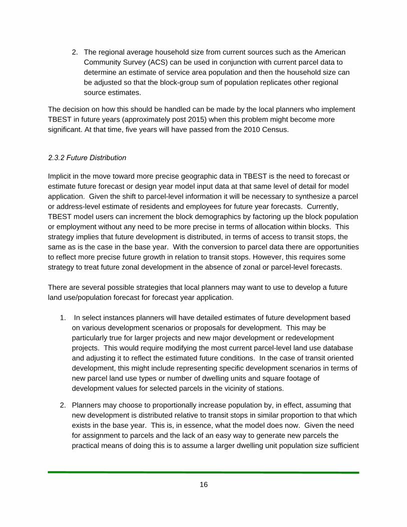
2. The regional average household size from current sources such as the American Community Survey (ACS) can be used in conjunction with current parcel data to determine an estimate of service area population and then the household size can be adjusted so that the block-group sum of population replicates other regional source estimates.

The decision on how this should be handled can be made by the local planners who implement TBEST in future years (approximately post 2015) when this problem might become more significant. At that time, five years will have passed from the 2010 Census.

2.3.2 Future Distribution Implicit in the move toward more precise geographic data in TBEST is the need to forecast or estimate future forecast or design year model input data at that same level of detail for model application. Given the shift to parcel-level information it will be necessary to synthesize a parcel or address-level estimate of residents and employees for future year forecasts. Currently, TBEST model users can increment the block demographics by factoring up the block population or employment without any need to be more precise in terms of allocation within blocks. This strategy implies that future development is distributed, in terms of access to transit stops, the same as is the case in the base year. With the conversion to parcel data there are opportunities to reflect more precise future growth in relation to transit stops. However, this requires some strategy to treat future zonal development in the absence of zonal or parcel-level forecasts. There are several possible strategies that local planners may want to use to develop a future land use/population forecast for forecast year application.

1. In select instances planners will have detailed estimates of future development based on various development scenarios or proposals for development. This may be particularly true for larger projects and new major development or redevelopment projects. This would require modifying the most current parcel-level land use database and adjusting it to reflect the estimated future conditions. In the case of transit oriented development, this might include representing specific development scenarios in terms of new parcel land use types or number of dwelling units and square footage of development values for selected parcels in the vicinity of stations.

2. Planners may choose to proportionally increase population by, in effect, assuming that new development is distributed relative to transit stops in similar proportion to that which exists in the base year. This is, in essence, what the model does now. Given the need for assignment to parcels and the lack of an easy way to generate new parcels the practical means of doing this is to assume a larger dwelling unit population size sufficient

17

to accommodate the forecast increase in population and then increasing the residential trip making as described later in this report.

3. If the population growth increment is known by block-group geography but there are insufficient data to discern how the distribution within a zone relative to transit stops might change, one strategy would be to determine an average population or trip rate distribution relative to transit stops from the base year dataset for various buffer densities. That distribution would then be applied to new zones with significant population growth (higher new average density). This might be relevant in locations where currently vacant areas are anticipated to be developed but specific plans are not in place on which to base dwelling unit assignment to parcels.

The actual strategy that local planners may choose to implement depends on local data availability as well as the magnitude and nature of anticipated future growth. The implementation of a strategy for determining future activity distribution as TBEST converts to parcel-level data are likely to increase the level of effort required by planners to prepare future year input data relative to the simply factoring process currently built into TBEST. The strategy outlined in number two above will be built into TBEST as the default strategy. Alternative strategies will require the local planners to produce an alternative future parcel-level dataset for model operation. 2.4 Employment

2.4.1 Conversion to Trip Attraction Currently the TBEST model (and virtually all travel models) uses employment as the data source for information about trip attraction to activities outside the home. While employment is a reasonable surrogate for work trip attraction, it is not a particularly good surrogate for total trip attraction to a site. Traditional models try to adjust for this by using some land use classification information and/or having various factors to balance production and attraction and forcing trip distributions to match roadway counts. For TBEST, while exploring this issue in conjunction with the issue of how to handle special generators, the project team chose to implement a strategy for TBEST to use parcel-level land use data to produce new surrogate measures for trip attraction that is essentially a measure of person trip attraction by parcel address. Transit stop buffer trip production/attraction is estimated by summing trip attraction from standard land use trip attraction data applied in conjunction with the parcel land use database. The discussion below details how this is carried out, first discussing employment allocation, then trip attraction allocation. Figure 8 outlines the various steps in the process.

18

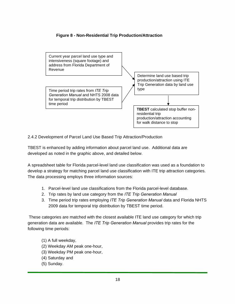
2.4.2 Development of Parcel Land Use Based Trip Attraction/Production TBEST is enhanced by adding information about parcel land use. Additional data are developed as noted in the graphic above, and detailed below. A spreadsheet table for Florida parcel-level land use classification was used as a foundation to develop a strategy for matching parcel land use classification with ITE trip attraction categories. The data processing employs three information sources:

1. Parcel-level land use classifications from the Florida parcel-level database. 2. Trip rates by land use category from the ITE Trip Generation Manual 3. Time period trip rates employing ITE Trip Generation Manual data and Florida NHTS

2009 data for temporal trip distribution by TBEST time period.

These categories are matched with the closest available ITE land use category for which trip generation data are available. The ITE Trip Generation Manual provides trip rates for the following time periods:

(1) A full weekday, (2) Weekday AM peak one-hour, (3) Weekday PM peak one-hour, (4) Saturday and (5) Sunday.

Figure 8 - Non-Residential Trip Production/Attraction

Current year parcel land use type and intensiveness (square footage) and address from Florida Department of Revenue

TBEST calculated stop buffer non-residential trip production/attraction accounting for walk distance to stop

Time period trip rates from ITE Trip Generation Manual and NHTS 2008 data for temporal trip distribution by TBEST time period

Determine land use based trip production/attraction using ITE Trip Generation data by land use type

19

The peak one-hour trip rates (for AM and PM peaks) are the trip rates during the hour of highest volume of traffic entering and exiting a site (during the AM and PM hours). Thus, these trip rates are not for the entire peak period, but during one hour of the peak period. Note that for some land uses, the trip rates are not available for some of the above-identified time periods. In these cases default strategies were used based on more aggregate data and the application of temporal travel trend data from NHTS. The trip rates from this table are used to compute the trip rates for each of the TBEST time periods. The time periods used in TBEST are:

Table 3 - TBEST Time Periods for Trip Rate

Period No Name of the Time Period Time Interval

1 Weekday AM peak period 6:00 - 8:59 AM

2 Weekday off- peak period 9:00 AM - 2:59 PM

3 Weekday PM peak period 3:00 - 5:59 PM

4 Weekday night period 6:00 PM - 5:59 AM (next day)

5 Saturday 12 midnight - 11:59 PM

6 Sunday 12 midnight - 11:59 PM

The trip rates are then computed as a function of the land use classification and availability of ITE data. A sample of the master table used in the translation of parcel land use classification to person trip production is shown as in Table 4.

20

Table 4 - Person Trip Rates Master Table (Sample Section)

Key Parcel

File Variable

Used to Drive

Trip Rates

Unit (Independent

Variable) Remarks

0=not

relevant for

transit,

1=Dwelling

Units,

2=Building Weekday Total

Weekday AM

Peak Hour

Weekday PM

Peak Hour

Calculated AM

Peak Period

Calculated PM

Peak Period

Saturday Total

Sunday Total

Vacant Residential Dwell ing Units 0 0 0 0 0 0 0 0

1 Single Family Dwell ing Units ITE LU ‐ 210 1 9.57 0.77 1.02 1.63 2.93 10.08 8.77

2 Mobile Home Dwell ing Units ITE LU ‐ 240 1 4.99 0.44 0.60 0.93 1.73 5.00 4.36

4 Condominiums Dwell ing Units ITE LU ‐ 230 1 5.81 0.44 0.52 0.93 1.50 5.67 4.84

5 Cooperatives Dwell ing Units ITE LU ‐ 220 1 6.65 0.55 0.67 1.17 1.93 6.39 5.86

3 Multi‐family ‐ less than 10 units Dwell ing Units ITE LU ‐ 221 1 6.59 0.51 0.62 1.08 1.78 7.16 6.07

8 Multi‐family ‐ 10 units or more Dwell ing Units ITE LU ‐ 222 1 4.20 0.34 0.40 0.72 1.15 4.98 3.65

6 Retirement Homes Dwell ing Units ITE LU ‐ 251 1 3.71 0.29 0.34 0.61 0.98 2.77 2.33

7Miscellaneous Residential (migrant camps,

boarding homes, etc.)Dwell ing Units

average of

260 and 2701 5.33 0.44 0.52 0.93 1.48 4.95 4.01

10 Vacant Commercial 1000 Sq.ft GFA 0 0 0 0 0 0 0 0

11 Stores, one story 1000 Sq.ft GFA 2 22.88 2.14 2.81 4.54 8.08 25.40 28.44

12Mixed use ‐ store and office or store and

residential or residential combination1000 Sq.ft GFA 2 17.23 1.97 2.27 4.18 6.53 3.05 3.42

13 Department Stores 1000 Sq.ft GFA 2 22.88 2.14 2.81 4.54 8.08 25.40 28.44

14 Supermarkets 1000 Sq.ft GFA 2 102.24 10.05 11.85 21.31 34.08 177.59 166.44

15 Regional Shopping Centers 1000 Sq.ft GFA 2 42.94 1.00 3.73 2.12 10.73 49.97 25.24

16 Community Shopping Centers 1000 Sq.ft GFA 2 42.94 1.00 3.73 2.12 10.73 49.97 25.24

17Office buildings, non‐professional service

buildings, one story1000 Sq.ft GFA 2 11.57 1.8 1.73 3.82 4.98 2.05 2.30

18Office buildings, non‐professional service

buildings, multi‐story2 23.14 3.60 3.46 7.63 9.95 4.10 4.60

19 Professional service buildings 1000 Sq.ft GFA 2 11.01 1.55 1.49 3.29 4.29 2.37 0.98

20Airports (private or commercial), Marine

terminals, piers, marinas1000 sq.ft

Non ITE

Source3 1.38 NA NA 0.23 0.34 0.25 0.2737

21 Restaurants, cafeterias 1000 Sq.ft GFA 2 127.15 13.53 18.49 28.69 53.17 158.37 131.84

22 Drive‐in Restaurants 1000 Sq.ft GFA 2 496.12 54.81 46.14 116.21 132.69 722.03 542.72

23

Financial institutions (banks, saving and loan

companies, mortgage companies, credit

services)

1000 Sq.ft GFA 2 148.15 17.31 26.69 36.70 76.76 86.32 31.90

24 Insurance company offices 1000 Sq.ft GFA 2 11.01 1.55 1.49 3.29 4.29 2.37 0.98

25Repair service shops (excluding automotive),

radio and T.V. repair, refrigeration service,

electric repair, laundries, Laundromats

1000 Sq.ft GFA 2 44.32 6.84 5.02 14.50 14.44 42.04 26.43

26 Service stations 1000 sq.ft 0 0.48 NA NA 0.08 0.12 0.57 0.79

27

Auto sales, auto repair and storage, body and

fender shops, farm and machinery sales and

services, auto rental, marine equipment,

trai lers and related equipment, mobile home

sales motorcycles, construction vehicle sales.

1000 Sq.ft GFA 2 47.63 3.31 4.61 7.02 13.26 1.59 2.30

28Parking lots (commercial or patron) mobile

home parks1000 Sq.ft 0 0. 91 0.08 0.11 0.17 0.30 0.83 0.74

29Wholesale outlets, produce houses,

manufacturing outlets1000 Sq.ft GFA 2 6.73 0.58 0.52 1.23 1.50 1.59 2.30

30 Florist, greenhouses 1000 Sq.ft GFA 2 40.20 5.63 4.99 11.94 14.35 57.38 39.45

31 Drive‐in theaters, open stadiums 1000 Sq.ft 3 0.77 NA NA 0.13 0.19 0.14 0.15

32 Enclosed theaters, enclosed auditoriums 1000 Sq.ft GFAFor

Multiplex 2 260.16 0.00 26.70 0.00 76.79 99.28 81.90

33 Nightclubs, cocktail lounges, bars 1000 Sq.ft GFA

Only

weekday

data

available.

2 86.75 0 15.49 0.00 44.55 32.14 35.99

34Bowling alleys, pool halls, Enclosed arenas,

Skating rinks1000 Sq.ft GFA 2 33.33 3.13 3.54 6.64 10.18 5.91 6.61

35

Tourist attractions, permanent exhibits, other

entertainment faci lities, fairgrounds

(privately owned).

1000 Sq.ft 3 2.08 0.07 0.27 0.14 0.76 2.24 1.87

36 Camps 1000 Sq.ft 0 0.26 0.01 0.02 0.03 0.07 0.05 0.06

37 Race tracks; horse, auto, dog 1000 Sq.ft 0 0.99 NA NA 0.17 0.24 0.18 0.20

38 Golf courses, driving ranges 1000 Sq.ft 0 0.12 0.01 0.01 0.02 0.03 0.13 0.14

39 Hotels, motels 1000 sq.ftNon ITE

Source2 5.74 NA NA 0.96 1.42 1.03 1.14

Table 3 Person Trip Rates Master Table (sample section)

ITE or Other Source Data ‐ Vehicle TripsDept. of

Revenu

e land‐

use

code

PROPERTY TYPE

TRIP RATE FROM ITE TRIP

GENERATION MANUAL

Commercial

Residential

21

For each land use category there is a key variable that is used as the metric on which trip production/attraction is based. The metrics are dwelling units (DU) for residential land use, and either structure area, typically expressed per 1000 square feet of structure, or land area similarly expressed. Occasionally ITE uses the number of employees as the metric for trip generation data collection. However, since data are not available in the property file for that category, alternative means are required to find comparable land use categories from which to derive trip production/attraction rates. Professional judgment is used to select comparable land use categories. Since the trip rates for orphanages, other charitable services (75), and for cultural organizations (79) are not available in the ITE Trip Generation Manual, we used the following source to obtain the trip rates: “San Francisco Interim Transportation Impact Analysis Guidelines for Environmental Review”, Interim Edition, January 2000, The Planning Department City and County of San Francisco. The virtues of using parcel land use data are not only the geographic precision and greater insight into the travel activities associated with the land, but empirical land use data which also provides insight into the temporal distribution of travel demand. For example, data can explain when travel demand occurs for various commercial and retail land use activities. Given TBEST has different models for different time periods; it provides an opportunity for the component models to be more accurately based on more specific time period data. The second set of columns in Table 4 illustrates the vehicle trip rates per unit of activity for each of the time periods and land uses. NHTS data were used to develop conversion factors from peak hour to peak period, enabling the use of the ITE peak hour data where available. Note that the spreadsheet from which Table 3 was taken includes all the land uses previously shown in Table 1, not just those shown in the sample table. Table 5 presents the temporal distribution of travel by trip purpose. Using professional judgment, each land use type has its trip production/attraction assigned to various trip purposes to understand the temporal distribution of travel. For example, an office facility would have some share of its travel assigned to work trip purposes as would be the case for office employees. Then some shares would be assigned for personal business or other purposes to represent the travel of the customers and clients that would be visiting the office property and interacting with the employees. Then, having an estimate of the temporal demand of the travel to and from the property, one can attribute the trip activity over the time periods for which TBEST has specific models. When looking at the temporal distribution, the model benefits in that the nature of activity over time periods becomes much more informative than when working with average daily information. For example, recreational venues would be expected to have greater activity on weekends and evenings and that distribution would be accordingly reflected in the estimates of trips for the respective time periods. Note that from the table below, total trip making on

22

Saturday is 97 percent of the amount on weekdays and Sunday travel is 82 percent of the amount on weekdays. Within the various trip purposes, however, there are far greater variances. For example, on Saturday work trip making (a key transit market) is only 33 percent of the weekday average whereas shopping, social recreation and travel for meals are all at least 50 percent greater on Saturdays compared to the average weekday.

Table 5 - Temporal Trip Distribution by Purpose

Sunday Monday Tuesday Wednesday Thursday Friday Saturday All

Home 17,427 19,342 20,051 20,043 19,675 19,875 18,405 134,819

Work 1,743 8,316 9,090 8,644 8,170 8,107 2,683 46,754

School/Daycare/Religious activity

4,464 2,720 3,129 3,951 3,104 2,977 946 21,292

Medical/Dental services 103 1,393 1,340 1,170 1,087 1,022 239 6,353

Shopping/Errands 9,123 9,374 8,701 8,828 8,930 10,105 13,884 68,944

Social/Recreational 7,426 5,681 5,889 5,524 5,900 7,253 9,740 47,413

Family personal business/Obligations

1,285 1,625 1,942 1,844 1,978 1,763 1,897 12,333

Transport someone 1,925 3,708 4,471 4,204 3,738 4,083 2,394 24,524

Meals 3,997 2,938 3,095 3,222 3,357 4,566 5,455 26,630

Other reason 231 354 282 493 576 439 300 2,675

All 47,724 55,451 57,990 57,923 56,515 60,190 55,943 391,737

Percent of Weekday Total

Sat as % of

weekday

Percent of

Saturday Total

Sun as % of weekday

Percent of Sunday Total

Home 34.4% 93.0% 32.9% 88.0% 36.5%

Work 14.7% 31.7% 4.8% 20.6% 3.7%

School/Daycare/Religious activity

5.5% 29.8% 1.7% 140.5% 9.4%

Medical/Dental services 2.1% 19.9% 0.4% 8.6% 0.2%

Shopping/Errands 15.9% 151.1% 24.8% 99.3% 19.1%

Social/Recreational 10.5% 161.0% 17.4% 122.8% 15.6%

Family personal business/Obligations

3.2% 103.6% 3.4% 70.2% 2.7%

Transport someone 7.0% 59.2% 4.3% 47.6% 4.0%

Meals 6.0% 158.8% 9.8% 116.3% 8.4%

Other reason 0.7% 70.0% 0.5% 53.9% 0.5%

All

97.1% 82.8%

Source: CUTR analysis of Florida NHTS data

23

The level of person trips to a parcel is a combination of all the people that travel there by all modes. Unfortunately, such data do not exist at the site or parcel level, hence, the reliance on data about vehicle trips from ITE as the primary source of activity levels at sites. It is acknowledged that this excludes activity that originated from walk, bike, transit and shared ride modes. Of those modes, the most significant is shared ride (passengers in vehicles traveling to and from the site). Bike, transit, and walk are generally minor modes. While it would be desirable to have data on parcel-level activity by these modes, in the absence of such data, the project team felt that using vehicle data still provides a huge increase in the amount of information that the Model has on which to base ridership forecasts. However, it is possible to account for shared ride travelers (occupants beyond the driver in cars) by converting the estimate of vehicle trips to an estimate of person trips. This adjustment involves using vehicle occupancy information to convert vehicle trips into person trips. To carry this out the project team used Florida NHTS data on occupancy by trip purpose and day to develop conversion factors. Table 6 illustrates the respective occupancy levels by trip purpose. The application of the various factors as outlined in the prior tables results in parcel and time period specific estimates of person trip production/attraction for each land use parcel. These then provide two key inputs for use in determining transit ridership. Accessibility to transit (activity levels in terms of person trips in vicinity of a bus stop) uses this information and accessibility via transit (activity levels accessible through the transit route network), also uses this data.

Table 6 - Vehicle Occupancy by Trip Purpose

Weekday - Personal Vehicle Occupancy

Purpose (Whytrp90) Weighted

To/from Work 1.33

Work Related 1.48

Shopping 1.78

Family/Personal 2.13

School/Church 2.08

Medical/DDS 1.76

Vacation 2.90

Visit Friends 2.01

Social Recreational 2.24

Other 1.99

Refused 2.03

Saturday - Personal Vehicle Occupancy

To/from Work 1.09

Work Related 1.28

Shopping 1.71


School/Church 1.72

Medical/DDS 1.54

Vacation 2.52

Visit Friends 1.84


Other 2.41

Refused 1.41

Sunday - Personal Vehicle Occupancy

To/from Work 1.17

Work Related 1.24

Shopping 1.80


School/Church 2.30

Medical/DDS 1.78

Vacation 2.47

Visit Friends 2.02


Other 2.33

Refused 1.36

Source: CUTR Analysis of NHTS Florida data

24

2.4.3 Future Distribution of Non-Residential Destinations Addressing future forecasts of trip attraction (the location of activities other than residential) are fraught with the same challenges noted above combined with the fact that analysts typically do not produce forecasts of future address-level employment and parcel-level land use. Accordingly, estimates of future trip attraction can be developed by the following options.

1. The planners can modify the land use parcel data file and the TBEST model will apply TBEST with the new forecast year data.

2. TBEST will retain the functionality to uniformly increase values for non-residential parcel trip attraction proportionally to a growth rate applied by the analyst. This might be based on forecast percentage increases in employment or economic activity.

3. The analyst could independently modify the trip rates and/or the demographics independently. In many ways this is a more theoretically correct way to understand what is going on. Historically, travel increases have been based on both population growth and increased travel per person with over half of the increase attributable to trip rate increases3. Future travel growth (or decline) will be attributable to changes in travel per person, typically highly impacted by real income changes, and by changes in the number of persons. Thus, one could modify both the number of parcels by type as well as the trip rates for the parcels to reflect changes over time. As changes in travel rates are modest over time it is not envisioned that such changes will be required in the near term.

3 Polzin, Steven, The Case for Moderating Growth in Vehicle Miles of Travel, 2006.

25

Chapter 3 - Data and Software Modifications 3.1 Introduction While this research effort was targeted to researching the implications of using parcel data; early in the work it was determined that this approach was promising and hence, work proceeded toward restructuring the TBEST software and datasets to allow the development of a version of TBEST that worked on parcel data as a prerequisite to attempting to calibrate the model. This required extensive efforts to modify the software in preparation for both the new data and the new calculations required to develop measures of access to transit and access via the transit network which are key components to the TBEST forecasting logic. The sections in this chapter below describe those modifications, and then the process for developing forecasting equations is described with results shown.

3.2 Data Requirements for Parcel Model The TBEST Parcel Model re-calibration effort provided an opportunity to address limitations within the previous TBEST model. One limitation included the inability to process more than one transfer path or incorporate greater than 85 minutes of maximum impedance into the model network accessibility calculations. Within the framework of the revised Parcel Model, the network accessibility code was modified to accept user-defined values for maximum transfers per trip and maximum trip impedance. This enhancement provides the user greater control over accessibility calculations that better fit the size and scale of the target transit system. For the Parcel Model calibration, the TBEST team concluded that 100 minutes of total impedance and a maximum of two transfers were adequate to simulate transit trip behavior patterns. The Parcel Model calibration depended on an updated set of demographic data to represent the reference year, 2009. In addition it was recognized that TBEST operation would require a data plan for use in post 2010 base-year and forecast-year environments to support Transit Development Plan (TDP) production. This resulted in extensive investigations and discussion of strategies for providing model data. This was complicated by the reduced availability of census data due to the decision to discontinue the long form census questionnaire that had been the source of several demographic variables that support TBEST, and further impacted by the fact that the American Community Survey (ACS) is far smaller and some block-group-level data are suppressed for some block groups due to concerns of disclosure. Thus, strategies were outlined that could provide data by defaulting to the next highest level of geography. The project team ultimately decided on a data plan as summarized in Table 7 below. Over time, as detailed Census 2010 data and 2006-2010 Summary ACS data become available these datasets can be assembled for use in TBEST over the next several years.

26

Table 7 - Data Plan for post 2010 TBEST Operation

Data Items 2010 Base Future Base Year

Updates Forecast Year

Transit network and schedule data

Directly entered into TBEST or from a Google specification

Directly entered into TBEST or from Google specification

Directly entered/edited in TBEST

Population count Block group Census for 2010

ACS data for smallest available geography allocated to block groups based on change in residential parcels

Percent increase input by analyst at block-group-level allocated across existing parcels

Population Race/ethnicity

Block group Census for 2010, ACS data

ACS 5-yr data No change from base

Population income, auto ownership etc.

2006-2010 ACS data at closest geography

ACS 5-yr data

No change from base

Parcel data 2010 parcel data from appraisers

Most current year data from appraiser (one year lag at most)

Base data unless modified by analyst.

The current TBEST model utilizes 2000 Census information and it is a known issue within the modeling community that moving to 2010 Census will be challenging due to the lack of data from the census long form which is no longer in use. To address this issue in the Parcel Model, the team developed state-wide 2009 Census demographic data from ACS data. While some Census 2010 block-level attributes were available, this information could not be used as the geography does not match that used for the 2005-2009 ACS data. Table 8 below summarized the ACS tables, data fields, and calculations used to develop the 2009 demographics utilized in the TBEST Parcel Model calibration dataset. Subsequent operation of the Parcel Model will require development of socio-demographic data for block groups based on a combination of data that will be available from the 2010 Census as well as from the 2006-2010 ACS.

27

Table 8 - Demographic Data Development for Base Year Demographic Conditions

Variable Census/ACS Table

Seq Cell values calculation

Description Available ACS geography level:

Block Update Block Group Update

Total Population

B01003

11 1 Total Population Block Group Pushed growth ratio for the block group down to the block

Value

Total Households

B11001

33 1 Household Type (Including Living Alone)

Block Group Pushed growth ratio for the block group down to the block

Value

Population 65+

B01001

10 ((20 + 21 + 22 + 23 + 24 + 25) + (44 + 45 + 46 + 47 +48 + 49)) / 1

Gender by Age Table: Added the male and female over 65 population divided by total population


NA

Population < 18

B01001

31 and 11

(3 + 4 + 5 + 6 + 27 + 28 + 29 + 30) / 1

Gender by Age Table: Added the male and female under 18 population divided by total population

Block Group Did not include in the model. We would have to include as an entirely new variable.

NA

Female Population

B01003

10 26 / 1 Total Population: Female population divided by total population


NA

Households in multi-family dwelling units

B11011

33 (5 + 10 + 14 + 18) / 1

Household Type By Units In Structure: Added all households with more than one unit and divided by total households

Tract NA Calculated ratio at the Tract level and pushed down to the block-group-level

28

Table8 continued - Demographic Data Development for Base Year Demographic Conditions Working Population

B08006 and B01003

25 and 11

1 / 1 Gender Of Workers By Means Of Transportation To Work: Total workers divided by total population.


Zero-vehicle Households

B08201

30 2 / 1 Household Size By Vehicles Available: Zero vehicle households divided by total households.


One-vehicle Households

B08201

30 3 / 1 Household Size By Vehicles Available: One vehicle households divided by total households.


Poverty Population

B17001

44 2 / 1 Poverty Status In The Past 12 Months By Gender By Age: Income in the past 12 months below poverty level divided by population for whom poverty status is determined


29

Table 8 continued - Demographic Data Development for Base Year Demographic Conditions Median household income

B19013

53 1 Median Household Income In The Past 12 Months (In 2009 Inflation-Adjusted Dollars):

Block Group NA Value

Per Capita Income

B19301

59 1 Per Capita Income In The Past 12 Months (In 2009 Inflation-Adjusted Dollars)

Block Group NA Value

Population foreign-born (latest 5 years)

B05012

19 3 / 1 Nativity In The United States: Foreign born population divided by total population


Black Population

C02003

12 4 / 1 Race Block Group Pushed growth ratio for the block group down to the block

NA

Hispanic Population

B03003

13 3 / 1 Hispanic Or Latino Origin [3]


NA

30

3.3 Incorporation of Parcel Data into TBEST Model Parcel Data Development The parcel data supplied as part of the parcel allocation process contained the required data to form a point (centroid) parcel spatial dataset that is the input to the TBEST model. To create this dataset, the x, y coordinate data fields included in the dataset were mapped in ArcGIS, projected to the TBEST coordinate system, and then input into the TBEST system geo-database. In addition to the input parcel dataset, several tables were created in the structure query language (SQL) Server database to store input data and processed data. Table 9 was created to house the parcel-specific data.

Table 9 - TBEST Data Table Summary

Table Name Description

PARCEL_RATE Land Use Trip rates identified by a unique code. Trip rates are available for each TBEST time period.

PARCEL_BUFFER Summarizes the Bldg. Sq. Ft., Land Sq. Ft., Dwelling Units, and Population for each stop in the network

PARCEL_TRIPENDS Summarizes the time period specific trips for each stop in the network specifically for the buffer characteristics

PARCEL_OVALUES Summarizes the time period specific trips for each stop in the network by land use code and O_value

3.3.1 Land Use Trip Rates Trips rates were stored in a spreadsheet developed as part of this project. The final trip rates corresponding to Florida Department of Revenue land use codes were imported into the Parcel_Rate TBEST data table. The import was performed by using SQL Server Data Transfer Services (DTS). Within the TBEST Parcel Model a code library was created to store the trip rates and then apply the rates based on input land use activity. The code library is utilized when calculating trips for stops and also when summarizing accessibility during the O-value calculations.

3.3.2 Association of Parcel Data to Network Stops The TBEST model run provides a multi-step process for associating socio-economic data to a network stop. This process was revised and improved to both incorporate parcel data and improve the socio-economic association using parcel locations. In previous versions of TBEST,

31

this process required a spatial auto-correlation process between the stop and the census geography to determine percent overlap of the stop buffer. In the Parcel Model, the model was revised to summarize socio-economic data associated with the parcels within the stop buffer using parcel density around the stop. During the model run process, parcels centroids are indexed to intersecting census block and block-group polygons. After this association is made, population, household and income information are determined by referencing the block or block- group data for each parcel within the stop buffer, summing the data, and dividing by the total number of parcels. This method focuses more on the actual density of market activity around the stop. During the calibration process, it was observed that calculated trip rates were high both at the trip end and the O-value calculations. It was determined that during the process to associate socio-economic and parcel data to the stop, some land use indicators were being double-counted by the model. In the previous version of TBEST, the socio-economic data were prevented from double-counting exclusively on stops with overlapping buffers on the same route. This was inadequate in the Parcel Model due to a point based distribution of data. To resolve the issue, double-counting was prevented for overlapping buffers on all stops with overlapping buffers around a subject stop. Within the process to associate parcel data to network stops, summarization of data requires a gravity function to decrease the impact of the parcel the further away it is from the subject stop. This process is the same as was utilized for point-based employment data in previous model versions.

3.3.3 Parcel Model Data Summarization and Output To summarize parcel data within the model, new code libraries were created to efficiently collect, process and store the data. Tabular parcel attributes include a land use code assigned by the Florida Department of Revenue, number of dwelling units, building square feet, land area square feet, and population data assigned from the allocation process. During a Parcel Model run, the new code libraries summarize the parcel attributes within a stop buffer for each land use category. The parcel code library then calculates trips associated with the subject stop based on the land use activity around the stop. Due to the large number of land use codes utilized by the model, it was necessary to condense the activities into three general categories of trip types: residential, visitor-based, and employee-based. In addition to summarization by land use type, the code library also summarizes parcel attributes based on these three groupings. The Parcel Model stores land use activity by identifying each unique land use code within stop buffer and summarizing the dwelling units, building sq. ft., land area, and population associated

32

with that land use code. These data are stored in the SQL Server PARCEL_BUFFER table. The model also calculates and stores the trips associated with each stop for each TBEST time period. While not all stored attributes are necessary for calculating trips, each attribute is currently stored for later summary and analysis. Trips calculated for each stop (trip-end) are stored in the SQL Server PARCEL_TRIPSENDS table. As mentioned previously, the model also calculates trips based on parcel data summarized for network accessibility. For each stop, the Parcel Model summarizes the land use activity for each TBEST O-value accessibility measure. The TBEST parcel code library is utilized to create a tabulation of dwelling units, building sq. ft., land area and population for each accessible land use code by O-value and TBEST time period. The tabulation is used to calculate the number of trips associated with the accessibility calculations. These tabulations are stored in the SQL server PARCEL_OVALUES table. 3.4 Model Preparations for Calibration The Parcel Model calibration process included the development of the data tables and code library described above. These new components were integrated with the existing TBEST 4.0 model. The JTA network was used as the input network to the calibration. Several model iterations were completed to test and devise the correct output for model estimation. The TBEST Loaded Network output was utilized to output existing variables for estimation. To output new parcel attributes, several new scripts were developed to semi-automate the process of transposing and formatting data for inclusion in the model estimation dataset. 3.5 Model Deployment The full-deployment of the TBEST model will require the following: Develop functions to update a transit system with parcel data and incorporate parcel

data in a new transit system Update target TBEST SQL Server databases to include system tables and views that

support parcel data storage and processing Modify and update the TBEST SQL Server table that stores model coefficients Update the TBEST model equation to incorporate Parcel Model coefficients Distribute the state-wide data package that includes 2009 Census data, 2010 InfoUSA,

and 2010 Parcels. Develop an algorithm to automate the incorporation of land use trip rates from the parcel

trip rates spreadsheet.

33

3.6 Parcel Model Data Issues The following issues were identified during the development of the Parcel Model. As the model distribution phase is implemented we will know more about how to better address these significant issues. Database Size Limitations - The TBEST Parcel Model creates a substantial amount of

data relating to parcel summary into trip-ends and accessibility values. Inserting this information will push the SQL Server Express database to its 1 GB limit as multiple scenarios are created. It will be necessary to mitigate the problem when we know the final required inputs to the revised model equation. Ancillary data can be either be kept in memory and then disposed of during the model run, or it can be kept in supporting text files that accompany each scenario. The text files would be accessed later during model summary or analysis. It is also possible that users would purchase a full version of SQL Server to overcome the 1GB size limit or that other database technology options such as cloud computing would fit the TBEST storage requirements.

Model Run Time – The model run time increases with the Parcel Model due to the additional processing incurred from the parcel data, modified maximum network impedance, and two transfers. The difference will be insignificant for small systems but could be significant for larger ones.

3.7 Estimation of TBEST Models The boarding equations in the new TBEST Parcel Model retain the current overall methodology and model structure, but significant changes have been made in terms of potential determinants of boardings in the individual boarding equations for the various type periods. The following are discussed in this section of the chapter: 3.8 Overall Methodology The methodology TBEST has developed is to ensure that the final boarding equations are sensitive to a wide range of demand and supply attributes. The following features of TBEST are particularly noteworthy:

1. Forecasting Stop-Level Boardings: TBEST provides forecasts or predictions of stop-level boardings. Thus, ridership in the context of TBEST is defined as the number of boardings at each stop that is specific to a direction and a route.

2. Direct vs. Transfer Boardings: TBEST incorporates separate equations for estimating

and distinguishing between direct boardings and transfer boardings at each stop. At any

34

given transit stop, one may have patrons who begin their trip at the designated stop and other patrons who are transferring from a different route in the middle of their trip/journey.

3. Time of Day Based Analysis: TBEST includes separate ridership equations by time

period within a week. The time periods that have been incorporated into TBEST include:

Weekday AM peak period

Weekday PM peak period

Weekday midday period

Weekday night period

Saturday (all day)

Sunday (all day)

4. Spatial Accessibility: TBEST accounts for spatial accessibility in computing boardings at individual stops. Presumably, ridership is dependent on the number of people of various characteristics (defined by age, working status, race/ethnicity, income, car ownership, etc.) who can access the transit system. TBEST considers circular buffer areas around individual stops to identify the market that has access to the transit system.

5. Time-Space Network Connectivity: In addition to considering spatial accessibility at the

origin stop, one needs to consider the overall connectivity and time-space accessibility that a system provides to accurately compute ridership at any stop. People are more likely to use a transit system (stop) that is well connected and from which many destinations offering a range of activity opportunities can be reached. However, it is likely that riders will not be willing to tolerate trip lengths or durations and transfers beyond a certain threshold level. Thus, one needs to consider the activity opportunities (measured in terms of population and employment) that can be reached within a certain time frame and number of transfers when modeling the number of boardings at any stop. In addition, this network accessibility needs to be computed and accounted for along the temporal dimension. The network connectivity and range of reachable destinations may be different at different times of the day due to supply differences by time of day. TBEST incorporates a powerful, comprehensive, and sophisticated methodology to account for time-space network connectivity and accessibility, thus making it the ideal tool for transit ridership forecasting.

6. Competing and Complementary System Effects: Within a transit system, there are

bound to be competing and complementary system effects that affect ridership. For example, any stop is likely to have a series of neighboring stops that are competing for the same market/riders. If neighboring stops have overlapping market area buffers, then

35

it is important to consider such competing effects in computing stop-level ridership. Similarly, there may also be complementary effects that affect and enhance ridership at a stop. For example, if a stop is a transfer point where two or more routes meet, then the number of boardings at the stop may be enhanced by virtue of the transfer opportunities present there. TBEST explicitly accounts for both of these effects in computing stop-level ridership.

7. GIS-Based Software Tool: TBEST has been developed so that the user can use the

software largely through an interface that provides full GIS functionality. Socio-economic scenarios, supply attributes, and route and stop configurations can be changed and edited on the fly, thus making TBEST a truly user-friendly transit ridership forecasting tool.

8. Performance Measures: TBEST includes estimates of several performance measures in

its output. Performance measures such as route miles, service miles, service hours, boardings per service mile or hour, and average boardings per service run are provided by TBEST at the individual route-level and for the system as a whole. These performance measures can be used to assess the impacts of various socio-economic and supply scenarios on system performance.

3.9 Model Structure

3.9.1 Network Relations Inter-relationships within a transit network really occur at the stop level. At a given stop along a particular route, boarding is influenced by whether there are other stops, either along the same route or other routes, within walking distance, from which potential users can get to the same destinations or different destinations. These other stops are referred to as the neighboring stops of the subject stop. More importantly, boarding at this stop is influenced by the opportunities that can be reached by potential users from each of these neighboring stops. If a potential user could reach a movie theater from any neighboring stop but not from the subject stop, the chance that this user would board at the subject stop for a movie trip is minimal. If a potential user can reach a movie theater from the subject stop with less time than from all neighboring stops, the chance of the subject stop being used is high. The stops accessible from the neighboring stops are referred to as the accessible stops. Among other factors, accessibility to opportunities around these accessible stops for potential activity participation can be critical in modeling and forecasting patronage at the stop level.

36

3.9.2 Neighboring Stops For a given stop (along a particular route in a particular direction), its neighboring stops are other stops within its buffer or whose buffers overlap with its buffer. These neighboring stops represent alternative points at which potential transit riders in the subject buffer may board a transit vehicle either on the subject route, in the subject direction of the subject route, or on other routes. The neighboring stops for a given subject stop fall into one of four groups: N0 through N3.

One set of neighboring stops are those on the same route and in the same direction as the subject stop. Some of these may be upstream of and some downstream of the subject stop. For either upstream or downstream, there may be multiple stops, depending on the density of stops in the subject direction along the subject route. While all of these potential neighboring stops can influence boarding at the origin stop, only the closest downstream stop is to be included in N1.

The second set of neighboring stops are those along the same route but in the opposite direction. There may be multiple of these potential neighboring stops. For actual measurement, however, only one is required. When there are multiple stops, the one closest to the subject stop is to be chosen as the N2 neighboring stop.

The N3 neighboring stops are those along other routes that are located within the subject buffer or within buffers that overlap the subject buffer. In any direction along any of these other routes, there may be multiple potential N3 neighboring stops. Again for computationally purposes, only one such stop from each combination of direction and route is to be included in N3. If two other routes intersect the subject route at the subject stop, for example, N3 would have four stops in most cases. It may have fewer than four if one or both of these intersecting routes are one-way.

The last set of neighboring stops, N0, is a subset of N3. They are neighboring stops on other routes and are located within the subject buffer. The reason to exclude those N3 neighboring stops located outside the subject buffer is that people that alight at them would need to walk more than the radius of a buffer to transfer at the subject buffer.

3.9.3 Accessible Stops With the four sets of neighboring stops determined, five sets of accessible stops are defined: S0 through S4. Assume that stop s serves direction d along route r.

Set S0 includes stops that can reach any of the N0 neighboring stops on other routes that are located within the subject buffer. The purpose of S0 is to capture passengers riding

37

toward stop s through other routes. That is, S0 represents feeders for potential transfer boarding at stop s. S0 is used later to measure the transfer potential for stop s. This transfer potential will be used in modeling transfer boarding but not in modeling direct boarding.

S1 includes stops downstream of stop s that can be reached from stop s through route r via the transit network. The purpose of S1 is to capture the opportunities for potential activity participation that are accessible for a potential user who boards at stop s or its N1 neighboring stops.

Set S2 includes stops in the network upstream of stop s through route r that can be reached from the N2 neighboring stop. S2 captures the opportunities for potential activity participation in the opposite direction of traveling at stop s through the same route as boarding at stop s.

Set S3 includes stops that can be reached from any of the N3 neighboring stops. S3 captures the opportunities for potential activity participation along other routes for people in the origin buffer. These three sets of accessible stops are used later to measure the accessibility to these opportunities for potential users in the stop s buffer.

Set S4 includes stops in S3 that overlap stops in S1. That is, people in the origin buffer can access some of the opportunities around each of the S4 stops from boarding at the origin stop or at any of the N3 neighboring stops. Overlapping stops refers to stops where the buffers overlap.

3.9.4 Direct Boarding Direct boarding for a given stop s and time period n is hypothesized to have the following equation:

, , , , , , , … ,

where

s = index for any origin stop.

n = index for any time period.

N = number of time periods.

snD = direct boardings at stop s during period n for the direction and along the route that

define stop s.

38

sC= vector of buffer characteristics for stop s. These characteristics include the amount

of population and employment as well as their characteristics.

snA1 = vector of accessibility to employment and population in the buffer areas of S1

stops during period n.

snA2 = vector of accessibility to employment and population in the buffer areas of S2 stops

during period n.

snA3 = vector of accessibility to employment and population in the buffer areas of S3 stops

during period n.

snA4 = vector of accessibility to employment and population in the overlapped buffer

areas S3 stops and S1 stops during period n.

snX = vector of other stop and route characteristics during period n.

3.9.5 Transfer Boarding Transfer boarding for a given stop s and time period n has the following equation:

, , , , , , , … ,

where

s

nT = transfer boardings at stop s during period n for the direction and along the route that define stop s.

snP0 = transfer potential from upstream boarding at S0 stops toward stop s during period

n.

s

nY = vector of other stop and route characteristics for period n. The amount of population and employment and their characteristics in the buffer of a subject stop are not directly relevant to transferring users. As a result, related variables are now replaced by the variable measuring transfer potential. It is possible that transit users may want to avoid transferring in buffer areas with certain characteristics, particularly in certain time periods. One good example is crime occurrence at night. However, data on such characteristics are rarely available. The vector of other stop and route characteristics in these equations may differ from those in the equations for direct boardings because some of these are irrelevant to transferring users. A good example is the presence of special generators.

39

3.10 Model Improvements Working with FDOT and others involved in developing TBEST, the research team identified a number of potential improvements for the ridership equations. These improvements have been considered and tested. They may eventually be implemented in a new model release depending on the statistical results from applying the JTA data to the model structure, and FDOT priorities for TBEST going forward. The most significant improvement is the use of trip ends for all modes and purposes. In the current ridership equations, one set of determinants is the socio-demographics and the amount of employment by type in the buffer of a subject stop. Another set of determinants is the accessibility to the amount of population and to the amount of employment by type to accessible stops from a subject stop. The third set of determinants is special generators as dummy variables. For the new equations, population and employment in the current direct boarding equations is replaced by a set of buffer characteristics that measure the number of trip ends by land use categories. The hypothesis that is that the number of trip ends is likely to be far more powerful than the amount of population and employment in forecasting direct boardings. But the socio-demographics is planned to be retained to reflect the fact that different population groups have different propensity of using transit even when the total amount of trip making is the same across these groups. The accessibility measures to population and employment for both direct and transfer boarding equations is similarly replaced by accessibility measures to trip ends. Another improvement is the splitting of overlapping buffers across different routes. In the current TBEST version, overlapping buffers along the same route are split to avoid double counting, but not between different routes. A third improvement relates to the treatment of service span for the weekday night period, Saturday, and Sunday. In the current ridership equations, service span for each of these periods enter the ridership equation as an exponential function, and experience indicates that this treatment of service span does not lead to robust ridership forecasting for significant changes in service span. The improvement is to specify the service span variable in the ridership equation in a particular way so that the resulting ridership equation can be used to forecast boardings per hour. This forecast of per hour boardings would then be expanded to get total ridership for an entire period by the actual number of service hours. Weights may be applied during this expansion process to account for that fact that hourly boardings can be significantly lower during the late night hours than during the evening and day hours.

40

3.11 Calibration Data Source The Jacksonville area was chosen for estimating the new ridership models. The main reason for this choice is that automatic passenger counts (APC) are widely used in the bus fleet and that APCs have been used for many years. The research team obtained data on employment, population, the socio-demographic characteristics of the population, and land use for the Jacksonville area as well as schedule and APC data for May 2009 from JTA. Schedule data were used to determine the number of vehicle arrivals for each stop (frequency), the vehicle travel time between consecutive stops, and service span for weekday nights, Saturday, and Sunday. The APC data were summarized to the individual one-way trip level. For a given stop and period, the APC data were used to determine the average number of boardings per vehicle arrival. The total number of vehicle arrivals for each stop and period was then used to expand the average number of boardings from the APC data to get an estimate of the total number of boardings for each stop and period. Modified TBEST was used to generate several variables for model estimation. These are transfer potential P0 and accessibility variables A1 through A4. 3.12 Estimation Process To estimate separate direct and transfer equations, all stops need to be divided into those that provide transfer opportunities and those that do not provide transfer opportunities. For a given stop, transfer opportunities exist when at least one stop on a different route is located within walking distance of that given stop. Model estimation is done in two steps. In the first step, the model for direct boardings is estimated using data from stops without transfer opportunities. In the second step, the estimated model for direct boardings is applied to all stops to predict direct boardings. For those stops with transfer activities, the predicted direct boardings is subtracted from the observed total boardings, and the difference is used as the dependent variable for estimating transfer boardings in the model. There are a large number of variations in specifying the ridership equations. These variations come from several sources:

Different statistical count models

Large number of potential socio-demographic variables for origin buffers

Multiple categories of land use types for measures of trip ends for both origin buffers and for accessibility measures

Model estimation requires selecting a statistical model that matches the nature of data at hand. Boardings at individual stops are a type of count data. Count data have two distinguishing features. One feature is that they are integers, and the other is that boardings are zero for a

41

large portion of stops. The commonly used linear regression model is inappropriate for count data. Instead, count data are typically modeled with Poisson and related statistical models. Poisson is the simplest but has a restrictive assumption that the mean and variance of the error terms are the same. Negative Binomial relaxes this assumption. More advanced models within this group deal with special features of count data. One special feature relates to whether the occurrence of zeros is actual behavioral or the result of sampling. The occurrence of zeros in the current dataset is unlikely to have resulted from randomness in data collection for two reasons. The first reason is that boarding data are from buses that have a high APC penetration rate. The second reason is that boarding data covers a period of only six months. As a result, this research focuses on Negative Binomial with Poisson as the backup in case Negative Binomial fails to converge. For each variation, one needs to consider how well a given statistical model fits JTA data. An important indicator for model fit is improvements in log-likelihood between a simple model with constants only and the full model. More importantly, one must consider whether the used variables are working properly. This includes two aspects. Do they show up in the equations in a statistically significant way? If they do, do they show up with the expected direction of effect on ridership? If they do, do they show up with numerically significant coefficients? 3.13 Estimation Results Table 10 illustrates the estimation results for both direct boarding and transfer boarding for each time period for bus stops only. Poisson was used to estimate the transfer-boarding equation for the AMPEAK period, while Negative Binomial was used for all other time periods and equations. The following highlights observations from these estimated equations.

The equations did not fit the data as well as expected. One important indicator for model fit is improvements in log-likelihood between a simple model with constants only, and the full model. The improvement in log-likelihood between “Restricted log likelihood” to “Log likelihood function” ranges from 7 percent to 32 percent in the direct boarding equations. The improvement is for the transfer boarding equations ranges from 13 percent to 72 percent.

The total number of trip ends and buffer characteristics in terms of share of population or households are included in the direct boarding only. The number of trip ends shows up with a positive coefficient for all periods. Different population segments perform differently in different time periods.

The accessibility to downstream destinations in terms of trip ends via the subject route (A1) is positive and statistically significant for both direct and transfer boarding.

42

How the accessibility to downstream destinations in terms of trip ends that can be reached both via the subject stop and via other routes/stops (A4) may impact boarding either way on a theoretical ground. Interestingly, A4 consistently has a positive effect on direct boarding, but a negative effect on transfer boarding.

There are two disappointments, however.

o First, the accessibility to alternative destinations in terms of trip ends through the opposite direction of the subject route or through other routes has been combined (A2+A3-A4) consistently shows up with a positive coefficient when statistically significant. As a result, it is not included in the equations shown in Table 10.

o Second, transfer potential P0 consistently shows up with a negative coefficient when statistically significant. As a result, it is not included in the transfer equations shown in Table 10. As a proxy, the number of nearby stops on other routes that people may transfer from to a subject stop is considered for the transfer equations, and has a positive and statistically significant effect for all time periods.

It is unclear at this point as to why these equations and key variables do not perform as well as one would have expected. It is clear, however, the reason is not the usage of trip ends in replacement of population and employment both for origin buffers and for destinations.

43

Table 10 : Equation - Model Estimation Results

Variables AMPEAK MIDDAY PMPEAK NIGHT Saturday Sunday

Direct Boarding Equations

Coeff. t-ratio Coeff. t-ratio Coeff. t-ratio Coeff. t-ratio Coeff. t-ratio Coeff. t-ratio

Constant -2.49656 -6.75 -2.40160 -8.10 -3.34923 -9.07 -4.78377 -7.33 -13.81903 -72.76 -15.09057 -28.23

All trip ends in origin buffer

0.00251 4.67 0.00132 8.07 0.00271 8.57 0.00838 4.64 0.00098 6.55 0.00071 5.54

Per capita Income in origin buffer

-0.00005 -6.84 -0.00002 -5.30 -0.00002 -3.66 -0.00008 -5.18 -0.00006 -8.06 -0.00005 -5.12

Share of workers in origin buffer

5.61808 7.25 4.75374 7.58 4.78785 6.14 3.51676 2.41 5.21811 4.25

Share of 0-veh households in origin buffer

3.78021 6.20 5.35325 10.77 6.46708 11.01 1.90955 1.71 4.04321 5.08

Share of Hispanic in origin buffer

3.88008 3.25

Share Multi-family dwelling units in origin buffer

10.70941 9.23

A1 to all trip ends 0.00107 5.71 0.00058 6.79 0.00048 4.71 0.00150 1.32 0.00069 3.67 0.00108 5.24

A4 to all trip ends 0.00440 2.75 0.00623 6.28 0.00316 3.59 0.09418 4.49 0.02795 6.21 0.02740 5.50

Observations 1,476 1,756 1,743 1,391 1,469 1,348

Log likelihood function

-2,446 -3,146 -2,182 -1,220 -3,219 -2,088

Restricted log likelihood

-2,845 -3,366 -2,596 -1,800 -3,773 -2,501

ρ squared 0.14 0.07 0.16 0.32 0.15 0.17

Transfer Boarding Equations

Coeff. t-ratio Coeff. t-ratio Coeff. t-ratio Coeff. t-ratio Coeff. t-ratio Coeff. t-ratio

Constant -0.47696 -16.52

-0.19426 -2.30 -0.75447 -9.39 -4.49070-40.53

-13.31899 -158.46

-12.57670-133.26

P0 from boardings on other routes

0.00557 7.12 0.00743 4.35 0.01252 6.66

Inbound stops on other routes

0.04126 8.28 0.04527 9.53 0.08034 11.46 0.04202 9.97 0.06971 12.59

A1 to all trip ends 0.00073 9.51 0.00053 4.38 0.00060 4.76 0.00251 3.01 0.00029 2.35 0.00030 1.73

A4 to all trip ends -0.00067 -1.91 -0.00291 -4.29 -0.00258 -5.16 -0.05211 -7.00 -0.00199 -2.04 -0.00625 -3.72

Observations 2,952 2,907 2,945 2,443 2,593 2,152

Log likelihood function

-6,409 -4,055 -3,499 -2,161 -5,633 -3,507

Restricted log likelihood

-22,627 -5,467 -4,640 -2,972 -6,504 -4,107

ρ squared 0.72 0.26 0.25 0.27 0.13 0.15

44

3.14 Model Coefficients For forecasting purposes, the direct-boarding model for a given period would first be applied to all stops to forecast direct boarding. For any given stop along a subject route, the forecast direct boarding at all stops along other routes that feed into the subject stop is then used to measure the potential for transfers at the given stop. The next step would be to forecast transfer boarding at stops with transfer opportunities. Total boarding would be the sum of the two. The re-estimated boarding equations should be applied with care. Consider the equations for the AMPEAK, PMPEAK, and MIDDAY periods first. For these three periods, the equations directly predict boarding for the whole period. Using direct boarding for the morning peak as an example, the following illustrates how these equations should be used. Direct boarding for the morning peak is expected to be equal to the exponential function of the following linear combination:

-2.49656 +0.00251 * All trip ends in origin buffer -0.00005 * Per capita income in origin buffer +5.61808 * Share of workers in origin buffer +3.78021 * Share of 0-vehicle households in origin buffer +0.00000 * Share of Hispanic in origin buffer +0.00000 * Share of multi-family dwelling units in origin buffer +0.00107 * A1 to all trip ends +0.00440 * A4 to all trip ends.

For the other three periods, including Night, Saturday, and Sunday, the equations as shown in Table 1 predict boarding per hour for both direct and transfer boarding. As a result, the predicted per-hour boarding must be multiplied by the corresponding service span in hours to get boarding for the entire period. Using direct boarding for Saturday as an example, direct boarding is expected to be equal to the product of service span in hours for Saturday and the exponential function of the following linear combination:

-13.81903 +0.00098 * All trip ends in origin buffer -0.00006 * Per capita income in origin buffer +0.00000 * Share of workers in origin buffer +0.00000 * Share of 0-vehicle households in origin buffer +3.88008 * Share of Hispanic in origin buffer +10.70941 * Share of multi-family dwelling units in origin buffer +0.00069 * A1 to all trip ends +0.02795 * A4 to all trip ends.

45

3.15 Implementation Steps Having modified the model to utilize parcel data and processing it to develop the input variables to drive development of the new forecasting equations, and having developed the new equations, subsequent implementation of the TBEST Parcel Model will involve inputting these new equations into the model and setting up the databases for future application. However, the implementation steps should include additional applications and sensitivity testing on another Florida property before release as an operational product.

46

Chapter 4 - Strategies for Treatment of Special Generators

4.1 Introduction A major challenge in enhancing the predictive capability of TBEST is to increase the amount of information available to adequately capture the activity levels (and hence, the transit trip generation characteristics) of different locations. Currently, population and employment are the only sources of information to represent the type and level of activity (hence, the level of transit trip generation) at different locations. Population counts may provide a reasonable amount of information to capture the trip production levels, because home end trip production at the household level vary relatively modestly and are known to be highly correlated with household characteristics. Further, such data are easily available to be incorporated into transit ridership equations. However, for the destination end of a trip the only information that is used as a surrogate for trip attraction is the activity level expressed in terms of employment by type. The range of employment types used in TBEST and elsewhere is very modest4 and the relationship between employment type and trip attraction is highly variable. While these employment types may capture the variation in transit trip attraction to a certain extent, several other factors may influence transit ridership. For example, several land uses such as airports, large shopping malls, hospitals, and universities may be categorized as “special generators” that are associated with unusually high trip generation characteristics compared to other land uses. Thus, employment (industrial, service, and commercial) alone may not sufficiently explain the transit ridership levels for such land uses. Currently, in TBEST, the only way to capture additional contributions to travel (beyond employment and population) due to special generators is by including dummy variables for special generators. This is because many types of land uses that have attraction for trip ends have no characteristic (other than a simple designation as a special generator in the form of a dummy variable) that can be integrated into the model. However, relying solely on dummy variables may not sufficiently capture the variation in transit ridership. It is desirable to move from representing special generators as dummy variables to expressing special generators in terms of variables that better capture the level of activity at the generators and that are more correlated with transit trip generation. Appropriate representation of special generators has been a long-standing issue in the travel forecasting field. However, this issue warrants much higher attention in the context of transit ridership forecasting and planning due to the higher propensity of transit serving special generators. In fact, it is not uncommon for special generator locations to be given special attention in the design and planning of transit networks and service.

4 In the current version of TBEST (and in many other models), three employment types are used: (1) Industrial employment, (2) Service employment, and (3) Commercial employment.

47

One objective of this research scope was to explore alternative ways to improve the representation of special generators to enhance the transit ridership prediction capabilities of TBEST. Specifically, the following directions were pursued:

(1) Search for “Transit Trip Generation Variables” for special generators that better represent the activity levels at special generators and better correlate with transit ridership.

(2) Use trip attraction measures from external sources as transit trip generation variables.

Each of the two pursuits are briefly discussed next.

4.1.1 Transit Trip Generation Variables for Special Generators One way to improve the predictive capability of the TBEST model is to improve the representation of special generators by moving from dummy variables to continuous variables that better capture the activity levels at the generators. Such “Transit Trip Generation Variables” can be used as explanatory variables (or independent variables) in TBEST model equations to explain the transit ridership at special generators. To this end, the project team conducted a literature review on how special generators are dealt with in regional travel demand models and in transit-related studies. This review helped in identifying the land uses that are commonly treated as special generators in a transit context. Further, this helped in identifying strategies on how to better represent special generators in the TBEST model rather than as mere dummy variables. This task also helped in identifying appropriate transit trip generation variables as well as data sources for those variables.

4.1.2 Integration of Trip Attraction Data from External Sources As indicated earlier, employment, population and special generator dummy variables are the only variables used in TBEST (and elsewhere) to measure the transit trip attractiveness (or accessibility) of a location. In addition to using employment, using trip attraction measures from other sources may help better explain stop-level transit ridership, especially for special generators. One source of trip attraction data are trip attraction measures available from existing regional travel demand models. However, travel demand models typically provide aggregate zone-level measures of trip attraction that are difficult to attribute to different special generators. Besides, TBEST is being moved from an aggregate, block-group-level (or zone-level) spatial resolution to disaggregate, parcel-level spatial resolution. The idea behind this move is that an accurate representation of the spatial distribution of input data (primarily, population and employment) can help improve the predictive capability of TBEST. This is because distance to a transit stop is an important determinant of the propensity to use transit (Neilson, 1972; Sullivan, 1996)

48

(hence the spatial distribution of activity centers relative to a transit stop is an important determinant of transit ridership at that stop). The move to the parcel-level spatial representation provides an opportunity to use parcel-level trip attraction measures that can better represent the activity levels at special generators. Such parcel-level measures of trip attraction can be created by integrating the parcel-level land use data (available from the Florida Department of Revenue) with empirical data on trip attraction levels by land use type (available in the Institute of transportation Engineers (ITE) Trip Generation Manual). It is worth noting here that the parcel-level trip attraction rates can be viewed as surrogate measures of the level of activity at each parcel-level land use. Thus, the move to parcel-level land use representation in TBEST and the use of parcel-level trip attraction measures is in some ways treating each (and every) parcel as a special generator. To the extent that the trip attraction rates represent the activity levels at each parcel that can be categorized as a special generator, the need for a better representation of special generators is addressed. The remainder of this report is structured as follows. The next section in this chapter provides a synthesis of the literature on how special generators are dealt with in travel modeling and transit ridership forecasting. Based on this review, a list of commonly used special generator land use categories is prepared, and the typically used measures to represent the intensity of activity at these special generators are compiled. The subsequent section in this chapter focuses on the second strategy outlined earlier and discusses the development of parcel-level land use based trip attraction measures for potential use in the TBEST model. The final section in this chapter discusses other alternative strategies that can potentially improve the capability of TBEST, either directly via enhancing the representation of special generators or indirectly. 4.2 Transit trip Generation Variables for Special Generators Special generators can be defined as land uses with unique (e.g., very high) trip generation characteristics than other land uses (Kurth et al., 1997). These are typically land uses with unusual (e.g., unusually large) concentration and/or type of activity-level, warranting special treatment for travel forecasting and transportation planning purposes. Examples of special generators include major shopping malls, large shopping stores, hospitals/medical centers, commercial airports, universities, high schools, colleges, elderly housing/nursing homes, amusement parks, sports stadiums, and other large recreation centers, military bases, park-and-ride lots, bus terminals, transit centers, and tourist attractions such as beaches. As indicated earlier, the TBEST model captures the additional (to employment and population) contribution of ridership due to special generators by including dummy variables for special generators. This is because many types of land uses that have attraction for trip ends have no characteristic that can be integrated into the model other than a simple designation as a special generator in the form of a dummy variable. However, only dummy variables may not sufficiently

49

capture the variation in transit ridership. Thus, it is desirable to move from representing special generators as dummy variables to special generators defined in terms of variables that better capture the level of activity at the generators and that are more correlated with transit trip generation. To this end, it is important to first understand how various regional travel demand models and transit analysis studies deal with special generators. Such a review will help in identifying the land uses that are commonly treated as special generators in a transit context, and in identifying appropriate transit trip generation variables as well as data sources for those variables. An exploration of regional travel demand models revealed the following ways in which special generators are treated in the travel demand modeling literature: (1) Separate trip production and attraction models are developed using trip generation rates

specific to each special generator (Pillar, 1997; Hull, 1998; Pickett, 2001; Cambridge Systematics, 2004; Kikuchi et al., 2004; Transportation Department of North Central Texas Council of Governments. “Dallas-Fort Worth Regional Travel Model Description.” June 2006.); and Wilbur Smith associates, 2008). These rates are either borrowed from other similar areas or developed from specifically collected data for special generators (traffic counts and characteristics of special generators, on-site counts, interviews, etc.). Trip generation models for special generators are typically developed using linear regression methods.

(2) Special generators are assigned specific rates of trip attraction (i.e., trip rates) obtained from the ITE Trip Generation Manual (KJS Associates, 1996; Lima & Associates, 2006; Pearson et al., 2009) or other similar sources for trip rates such as the San Diego Municipal Code, 2003. Specifically, trip attraction due to special generators is estimated using the trip rates for corresponding land-uses from the ITE Trip Generation Manual. The trip rates are expressed in terms of the number of trips per trip generation variable. A “trip generation variable” is an independent variable (e.g., employment, square footage of the land use) that explains the trip attraction at that special generator.

The above discussion is based on the review of literature in a regional travel demand modeling context. In the context of transit ridership analysis, however, there is very limited published literature on the subject of special generators. These studies are discussed below. A study by Kurth et al. (1997) analyzes the impact of special generators on transit services. This study divides special generators into three groups based on the regularity of the activity at the generators: (1) Regular special generators are those special generators that produce trips on a regular,

weekday basis. Examples include airports, regional shopping centers, hospitals, schools, colleges, and park-and-ride lots.

50

(2) Periodic special generators are those generators that do not produce trips on a regular weekday basis. Examples include convention centers, stadia and arenas, parks, fairs and festivals. Kurth et al. suggests the use of data on attendance per day (obtained from either on-site surveys, or the management of the special generator) to estimate transit trip attraction by such periodic special generators.

(3) “Special” special generators include those sites or activities that cannot be easily classified as regular or periodic special generators.

A report by Boyle (2006) suggests the development of trip generation models for special generators akin to the trip generation models in regional travel demand models, and then applying a mode split model to obtain the transit trip attraction data. A study by Parsons Brinckerhoff (2000) captures transit trip attraction for medical services such as hospitals based on the number of beds in the hospital and for colleges based on the number of students enrolled. A report by The Duffey Company (2000) identifies the potential special generators for transit analysis by analyzing the transit trip rates information that was specifically developed by conducting transit ridership surveys at special generators. Review of the above-mentioned transit-specific special generator studies indicates that locally collected data are typically used to explain transit ridership due to special generators. Such data are collected through on-board surveys (Parsons Brinckerhoff, 2000) and on-site surveys or interviews (Kurth et al., 1997; The Duffey Company, 2000; Usvyat et al., 2009). A project report on “Understanding Transit: Basic Course Material on Public Transportation” by the Center for Urban Transportation Studies, University of Wisconsin-Milwaukee suggests site interviews at special generators as an important source of data for transit analysis. Such interviews are helpful in measuring the size (number of visitors, employment, area, etc.) of, and ridership at, special generators. Another paper by Carter (1985) also emphasizes the importance of such special generator information in transit and traffic analysis. The paper presents detailed recommendations on questionnaire content and procedures. According to a report by LSA Associates, Inc. (2008), review and application of special generator developments is one of the important aspects in developing travel demand models. According to their recommendations, first, potential special generators need to be identified and categorized into broad categories such as event centers, airports, stadiums, resorts, theme parks, religious places, tourist destinations etc. based on the type and size of the generator. Second the following information on special generators needs to be collected:

(1) Description and location of activity

(2) Duration and recurrence of activity (e.g., random vs. scheduled, one-time vs. daily)

(3) Category of the special generator

51

(4) Trip distribution and mode choice information

(5) The seasonal variability of trip-making

(6) Independent trip generation variables and their availability

They also emphasize that the most important data needed to characterize the transit ridership characteristics of a special generator are the independent trip generation variables as they define the trip attraction capability of the generator. Following the above recommendations (and other studies reviewed), we first identified a list of commonly used special generator categories along with the commonly used measures of activity at each special generator. Table 11 presents the list of identified special generator categories. For each special generator category, the corresponding trip rates from the ITE Trip Generation Manual, a list of commonly used variables to explain activity level at these special generators, and relevant literature are provided. The special generators mentioned in Table 11 were selected based on their likelihood to attract transit trips (based on literature and professional judgment). The first part of Table 11 with the heading “Trip Rates from ITE Trip Generation Manual” provides the trip rates for each special generator category using the ITE Trip Generation Manual, 8th Edition. The trip rates were obtained by matching each special generator category with the closest available ITE land use category. The trip rates are available for various independent variables on a Weekday, Saturday and Sunday. The other part of Table 11 with the heading “Variables Used to Explain Special Generator Trip Generation in the Literature” includes a brief description of each study in the literature on how it deals with a special generator and a list of variables used in that study to explain trip attraction at that generator. More details on each of these reviewed studies are available in Appendix A.

52

5 For airports, ITE trip generation manual provides transit trip generation rates as well as vehicle trip rates. The transit trip rates are valuable in that they can be used as measures of transit ridership attractiveness of airports. For all other land uses the ITE trip rates are vehicle trip rates, not transit trip rates. Average weekday transit trips for commercial airports given by ITE trip generation manual are as follows: 4.97 per employee, 48.8 per average flight, and 41.3 per commercial flight.

Table 11- Tabulation of Special Generators with ITE Trip Rates, Relevant Studies and Corresponding Variables Used

Sr. No

Special Generator Category

Trip Rates from ITE Trip Generation Manual Variables Used to Explain Special Generator Trip Generation in the Literature

Unit [Independent Variable(X)]

On a Average Trip rate

/ unit

Fitted Curve

Equation

List of Variables Used

Study Description

1 Commercial

Airports5

Employees

Weekday 13.4 -- Number of Boardings (Enplanements).

Baik et al. (2008) developed a trip generation model to estimate number of person trip attracted by using number of enplanements as an independent variable in the regression analysis. Trip attraction is obtained for 66 international airports in U.S by using data from Bureau of Transportation Statistics T100 international segment database.

Saturday 12.2 --

Sunday 14.7 --

Average Flights per Day

Weekday 104.73 -- Number of Deplaning Passengers. Number of Boardings

In the Laredo Travel Demand Model prepared by Wilbur Smith Associates (2008), trip attraction for international airport is estimated based on the number of deplaning passengers and number of boardings. Trip attraction model was developed using linear regression analysis.

Saturday 98.46 --

Sunday 119.61 --

No. of Employees In the Lincoln MPO Travel Demand Model, ITE Trip Generation Manual, 7th Edition is used to calculate the trip attraction. Trip attraction for airports are obtained based on the number of employees in the airport.

Commercial Flights per Day

Weekday 122.21 --

Saturday 113.04 --

Number of Boardings

2007 Passenger Boarding and All-Cargo Data maintained by Federal Aviation Administration (FAA) can be used for the trip generation model. This dataset contains total number of boardings for the Commercial Service Airports (at least 2500 passenger boardings/year). This data only gives annual boarding at commercial service airports. Also, FAA’s Terminal Area Forecast (TAF) can be used to obtain the historical and forecast data on boardings (enplanements) for active airports in the National Plan of Integrated Airport Systems (NPIAS).

Sunday 137.71 --

2

Major regional

amusement parks

Employees

Weekday 8.33 -- Acreage of the Park. No. of Visitors / day.

In the Laredo Travel Demand Model prepared by Wilbur Smith Associates (2008), trip attraction for regional parks is estimated based on the number of visitors/day and acreage of the park. Linear regression analysis was performed using data from the traffic counts.

Saturday 22.08 --

Sunday 20.96 --

Acres

Weekday 75.76 -- Acreage of the Park

In the Michigan Statewide Travel Demand Model prepared by KJS Associates (1996), trip attraction for parks is computed by developing trip attraction rate based on the acreage of the park obtained using ITE Trip Generation Manual.

Saturday 180.2 -- Total attendance per day.

Kurth et al. (1997) developed a four step model to estimate the annual transit trips attracted by amusement parks. Trip generation, trip distribution, mode choice and transit assignment models were used based on the data (attendance per day) obtained from the local surveys.

Sunday 171.02 --

53

Table 11 Continued

Sr. No


Trip Rate from ITE Trip Generation Manual Variables Used to Explain Special Generator Trip Generation in the Literature Unit

[Independent Variable(X)]


/ unit

Fitted Curve

Equation


Study Description

3

Major sports

facilities - Stadia,

Arena etc

Employees Weekday 10 -- Capacity of the Facility.

In the Laredo Travel Demand Model prepared by Wilbur Smith Associates (2008), trip attraction for regional sports facilities is estimated based on the capacity of the facility. Trip attraction model was developed using linear regression analysis.

Acres Weekday 33.33 -- Total Attendance per event

Kurth et al. (1997) developed a four step model to estimate the annual transit trips attracted by stadiums. Trip generation, trip distribution, mode choice and transit assignment models were used based on the data (attendance per event) obtained from the local surveys.

4 Recreational community

center

Members Saturday 0.07 --

Area of the facility (1000 Sq.ft).

City of San Diego has developed its own Trip Generation Manual. Trip rates for each land use were obtained by conducting detailed local surveys (vehicle trips) at various sites of each land use type. Vehicle trip rate for Recreational Building is 45 trips/1,000 sq. ft.

Sunday 0.15 --

Employees Weekday 27.25 -- Saturday 18.34 -- Sunday 12.03 --

Gross Floor Area (1000 Sq.ft)

Weekday 22.88 -- Saturday 9.1 -- Sunday 13.6 --

5 High school

Students Weekday 1.71

0.81 Ln(X) + 1.86 Student

enrollment Number of staff.

In the Laredo Travel Demand Model prepared by Wilbur Smith Associates (2008), trip attraction for high school is estimated based on the number of students and number of staff. Linear regression analysis was performed using data from the survey of high schools.

Saturday 0.61 --

Gross Floor Area (1000 Sq.ft)

Weekday 12.89 --

Saturday 4.37 --

Student enrollment

School Enrollment data are collected annually in the October Current Population Survey (CPS) and can be used for the trip attraction model. http://www.census.gov/population/www/socdemo/school.html Employees

Weekday 19.74 1.13 Ln(X)

+ 2.31 Saturday 6.57 --

6 College / University

Students§ Weekday 2.38

2.23(X) + 440

Student enrollment

Parsons Brinckerhoff (2000) developed a gravity model to estimate potential intercity transit demand in Arizona. It captured the transit trip attraction for college by using the data on number of students enrolled obtained from the survey.

Student enrollment Number of staff.

In the Laredo Travel Demand Model prepared by Wilbur Smith Associates (2008), trip attraction for college/university is estimated based on the number of students and number of staff. Linear regression analysis was performed using data from the survey of colleges/universities.

Saturday 1.3 --

Number of Employees.

In the Dallas-Fort Worth Regional Travel Model, trips attracted by college/university is computed by applying the trip attraction rates to the employment and adding extra increment trips associated with college/university . The number of incremental trips for college/university is obtained by taking the difference of cross classification model generated trip rates and trip rates obtained from regional travel survey. Employees

Weekday 9.13 0.74(X) +

3.92


In the Lincoln MPO Travel Demand Model, ITE Trip Generation Manual, 7th Edition is used to calculate the trip attraction. Trip attraction for university main campus is obtained based on the number of employees. Saturday 3.12 --

54

Table 11 Continued

Sr. No


Trip Rate from ITE Trip Generation Manual Variables Used to Explain Special Generator Trip Generation in the Literature

Unit [Independent Variable(X)]


/ unit

Fitted Curve

Equation


Study Description

7 Hospital

Beds

Weekday 11.81 7.42(X) + 1733.31

Number of Beds

Parsons Brinckerhoff (2000) developed a gravity model to estimate potential intercity transit demand in Arizona. It captured the transit trip attraction for medical services such as hospitals by using the data on number of beds in the hospital obtained from the survey

Number of Employees. Number of Beds.

In the Laredo Travel Demand Model prepared by Wilbur Smith Associates (2008),trip attraction for hospital/medical center is estimated based on the number of employees and number of beds. Linear regression analysis was performed using data from the survey of hospitals/medical centers.

Saturday 8.14 0.58 Ln(X)

+ 4.65

Sunday 7.19 0.61 Ln(X)

+ 4.38

Employees

Weekday 5.2 4.4(X) + 711.46


In the Lincoln MPO Travel Demand Model, ITE Trip Generation Manual, 7th Edition is used to calculate the trip attraction. Trip attraction for medical centers is obtained based on the number of employees. Also, the Whatcom County Travel Demand Model captures the trip attraction for hospitals using the information on the number of employees in each hospital.

Saturday 3.78 2.95(X) +

691.43

Sunday 3.34 2.56(X) + 663.23

Gross Floor Area (1000 Sq.ft)+

Weekday 16.5 10.13(X) + 2191.79

Number of Beds American Hospital Association (AHA) collects data on number of beds for more than 6500 AHA registered hospitals throughout the United States. This dataset is available at state and regional geographic level and can be used.

Saturday 10.18 0.43 Ln(X)

+ 5.79 Number of Employees.

In the Dallas-Fort Worth Regional Travel Model, trips attracted by a hospital are computed by applying the trip attraction rates to the employment and adding extra increment trips associated with the hospital. The number of incremental trips for a hospital is obtained by taking the difference of cross classification model generated trip rates and trip rates obtained from regional travel survey.

Sunday 8.91 3.53(X) + 1937.21

8 Shopping

Center (SC) Gross Leasable

Area (1000 Sq.ft)

Weekday 42.94 0.65 Ln(X)

+ 5.83 Number of Parking Spaces. Number of Stores. Type of Stores. Floor area of SC.

Kikuchi et al. (2004) developed macroscopic and microscopic model to estimate the attraction rate of a SC. In macroscopic approach, relationship between the listed variables & attraction rate was obtained using regression analysis and in the microscopic approach, attraction rate of the SC was taken as weighted sum of attraction rates of individual stores. The data used in both the approaches was obtained by the surveys conducted at various shopping centers. Saturday 49.97

0.63 Ln(X) + 6.23


In the Lincoln MPO Travel Demand Model, ITE Trip Generation Manual, 7th Edition is used to calculate the trip attraction. Trip attraction for malls is obtained based on the number of employees.

Sunday 25.24 15.63(X) + 4214.46 Number of

Employees.

In the Laredo Travel Demand Model prepared by Wilbur Smith Associates (2008), trip attraction for a shopping center is estimated based on the number of employees. Linear regression analysis was performed using data from the traffic counts done at various shopping centers.

55

We also identified the independent transit trip generation variables that can be used to explain transit ridership at each generator, as shown in Table 12 below. The explanatory variables listed in this table were obtained based on the literature review, professional judgment of the project team, and the ease of availability from different data sources.

Table 12 - List of Explanatory Variables of Each Generator

Special Generator Category Options for Explanatory Variables

Best Next Best Other

Commercial Airports Daily Boardings/ Enplanements, Daily Flight Arrivals/Departures

Employees -

Major Regional Amusement Parks

Visitors/day Parking Spaces

Employees or acres

Major Sports Facilities Total Attendance/event Capacity (seats)

Parking Spaces

Recreational Community Center Visitors/day Parking Spaces

Area (1000 Sq.ft)

High School Students Enrolled Employees -

College/University Students Enrolled Employees -

Hospitals Number of Beds Employees -

Shopping Centers (SCs) Employees Parking Spaces

Floor Area of SC

Free Standing Superstore Area (1000 Sq.ft Gross Floor Area)

- -

Park-and-Ride Lots with Transit Service

No. of Parking Spaces

Service Area Population Ratio of Auto Costs to Transit Costs. Distance from Park-and-Ride Facility to Major Employment Centers. Number of Express Buses during the Morning (AM) Peak. Best (not average) Time Between the Park-and-Ride Facility and the Central business district. Presence of Nearby Park-and-Ride Facilities. Availability of Midday Service.

56

For some of the special generator categories – schools/colleges/universities, airports, and hospitals – several data sources were identified to obtain information on useful trip generation (explanatory) variables. These data sources are briefly discussed below, with more details presented in Appendix B. (1) Schools, colleges and universities: Student enrollment best describes the trip generation at

these places. This data can potentially be obtained from the following datasets: 2000 U.S Census data, Current Population Survey (CPS) and American Community Survey (ACS) data.

(2) Airports: Annual passenger enplanement for commercial service airports can be obtained from the Federal Aviation Administration (FAA) - Passenger Boarding (Enplanement) and All-Cargo data. This dataset is easily available for the current year and the next fiscal year. Further, FAA’s Terminal Area Forecast (TAF) can also be used to obtain historical and forecast data for enplanements. This dataset includes forecast for FAA towered airports, federal-contracted towered airports, non-federal towered airports, and many non-towered airports. The 2009 database provides forecasts for boardings (enplanements) from 2010 to 2030.

(3) Hospitals: The American Hospital Association (AHA) annual survey database can potentially be used. This dataset provides the number of beds for more than 6500 AHA registered hospitals throughout the United States. These data are available at the state and the regional geographic level. The dataset can be purchased in the form of a compact disc or a book.

The above identified data sources can be readily used to obtain information on the base year activity levels (trip generation variable) of the special generator. However, the future estimates required for forecasting purposes are available only for airports. Specifically, the 2009 FAA’s TAF database can be used to obtain the enplanement forecast from 2010 to 2030. Availability of explanatory variables data for long-term forecasting purposes remains a challenge. Nonetheless, for short-term forecasting purposes, the above-mentioned data sources can be valuable. In addition to the above mentioned data sources, transit agencies can compile their own data from various locally available data sources, as well as conduct specialized surveys to collect information on transit trip generation variables for different special generators. If a transit agency undertakes such specialized data collection efforts, collecting data on the variables identified in Table 12 is likely to be most beneficial for any transit ridership analysis/forecasting exercise.

57

4.3 Parcel-Level Land Use Based Trip Attraction Measures As indicated earlier, the move to parcel-level spatial representation provides an opportunity to use parcel-level trip attraction measures that can better represent the activity levels at special generators. To this end, parcel-level measures of trip attraction have been created by integrating the parcel-level land use data (from the Florida Department of Revenue) with empirical data on trip attraction levels by land use type (available in the ITE Trip Generation Manual).

4.3.1 Property Appraisal Parcel-Level Land use Data Pparcel-level land use data used for this procedure were created from the 2009 Property Appraisal data for the state of Florida, obtained from the Florida Department of Revenue (DOR). The data includes about 100 land uses broadly classified in to residential, industrial, commercial, agricultural, institutional, government and miscellaneous categories based on the land use at the property. The database contains information on land use, property type, area, physical address, land value etc. Each property is called as a parcel, described based on ownership and land use. For each parcel, information on its geographic location and address, size (square footage of the land and the building on it), year built, number of buildings, the land value etc. is available. 4.4 Trip Rates from the ITE Trip Generation Manual The ITE Trip Generation Manual, 8th Edition used for the development of trip rates consists of two data volumes with land use descriptions, vehicle trip generation rates, equations and data plots. Volume I contains the trip generation rates, and regression equations for a variety of land uses coded 000 through 499. These include the broad land use categories Port and Terminal, Industrial/Agricultural, Residential, Lodging, and Recreational. Volume 2 contains the trip generation rates, and equations for land uses coded 500 through 999, which include Institutional, Medical, Office, Retail, and Services categories. The trip rates reported in these volumes are based on data from more than 4800 sites. Most of the trip rates are available for one or more of the following time periods: (1) weekday, (2) weekday AM peak one-hour6, (3) weekday PM peak one-hour, (4) Saturday and (5) Sunday.

6 The peak one hour trip rates (for AM and PM peaks) are defined as the weighted average vehicle trip rate during the hour of highest volume of traffic entering and exiting the site (during the AM and PM hours).

58

4.5 Procedure to Develop Parcel-level Trip Attraction Measures For each non-residential land use category (DOR land use code greater than 10) in the parcel-level land use data, the trip rates for the corresponding ITE land use categories were used. Table 13 provides such trip rates obtained from the ITE Trip Generation Manual for each land use category in the parcel-level data. The first part of the table with the heading “Trip Rate from ITE Trip Generation Manual” provides the trip rate for each land use using The ITE Trip Generation Manual, 8th Edition. The first column under this heading indicates the independent variable used to provide the trip rates. For example, 1000 sq ft Gross Floor Area (GFA), indicates that the reported trip rates in that row are per 1000 square feet of the GFA of the parcel. These trip rates can be multiplied with the total GFA (in 1000 square feet) of the parcel to obtain a measure of the trip attractiveness of the parcel. Below are some notes on the procedure used to obtain trip rates for each parcel-level land use category. (1) The trip rates were obtained by matching each parcel-level land use category with the

closest land use category in the ITE Trip Generation Manual (a one-to-one mapping).

(2) Several parcel-level land use codes include multiple ITE land use categories under one single (parcel-level) land use code. In such cases of a one-to-many correspondence from parcel-level land use codes to ITE land use categories, the ITE trip generation rates were averaged across the land uses. For example, florists and greenhouses are included within a single parcel-level land use code (030)7. The trip rate for this land use code was obtained by taking an average of the ITE trip rate for florists and the ITE trip rate for greenhouses. The same strategy has been used for several other land use categories such as motels and hotels (039), and auto sales and auto parts (027).

(3) Under some parcel-level land use codes, rather disparate types of land uses are clumped. For example, airports, marinas, and other water terminals were classified into a single parcel-level land use code (020). These land uses are significantly different from each other in terms of their trip generation characteristics. In such cases, the table provides separate trip rates for each of the different land uses categorized under a single land use code.

(4) For parcel-level land use codes (such as restaurants and parks) that are classified into many types in the ITE Trip Generation Manual (i.e., a many-to-one correspondence), the maximum value of the trip rates of the different ITE land uses is reported. For example, ITE trip rates are available for two types of restaurants (021) – high-quality restaurants and high-

7 Numbers in parentheses show the parcel-level land use code

59

turnover restaurants. The trip rate of high-turnover restaurants (which is higher than that of the high-quality restaurants) is reported in this case.

(5) Several parcel-level land use categories do not have trip rates available by square footage in the ITE Trip Generation Manual. For example, the airports category (020) does not have trip rates per square footage. Therefore, trip rates for such land use categories are given with respect to other explanatory variables available in the ITE Trip Generation Manual. Other land uses such as service stations (026), race tracks (037), golf courses (038), hotels & motels (039), homes for the aged (074) and military base (081) have the same issue.

If the trip rate is not available for a particular time period, it is marked as NA (Not Available) in the cell corresponding to that land use and time period. As it can be noted from the columns under the heading “Trip Rate from ITE Trip Generation Manual” in Table 12 above, the ITE Trip Generation Manual provides daily trip rates separately for weekdays, Saturdays, and Sundays, and its own definitions of different time periods (AM peak, PM peak) in a weekday. These time periods do not match with those of the time period definitions used in TBEST. To obtain the trip rates by different time periods appropriate for the TBEST model, temporal variation of trips in the temporal variation of trips in the 2001 NHTS database was utilized. The second part of Table 12 with the heading “Trip Rate Based on ITE Trip Generation Manual and 2001 NHTS database for TBEST Time Periods” gives the trip rate of each land use for all the TBEST time periods. Below are some notes on the procedure used to convert ITE trip rates to trip rates for TBEST time periods.

In this part of the table, the columns “Weekday AM Peak Period” and “Weekday PM Peak Period” are split into two columns each – “Using temporal distribution of trips in NHTS” and “Using Peak Factors”. The trip rates in these two columns have been computed using two different methods, as described below:

Method 1: By multiplying the weekday trip rates obtained from the ITE Trip Generation Manual with the temporal distributions of weekday trips in the 2001 NHTS database shown in Table 13 below.

Table 13 - Temporal Distribution of Weekday Trips in 2001 NHTS Data

Period No. Weekday Time period Percent

1 6am to 8:59 am (AM peak period) 16.8

2 9:00 am to 2:59 pm (Off-peak period) 35.4

3 3:00 pm to 5:59 pm (PM peak period) 24.8

4 6:00 pm to 5:59 am (Night period) 23.1

Method 2: By multiplying the peak one-hour trip rate from ITE Trip Generation Manual to the peak factor obtained from the 2001 NHTS database. Peak factor was computed by

60

taking the ratio of the number of trips in the peak period to number of trips in the peak one-hour of the peak period.

Between the two methods mentioned above, trip rates obtained using peak factors (Method 2) should be used because this methodology is more specific to the various land uses as compared to using the temporal distribution of 2001 NHTS database. But some of the parcel land uses mentioned below have peak hour periods different from the TBEST time periods. Table 14 below illustrates those land uses.

Table 14 - Parcel Land Uses Having Peak Hour Period Different from TBEST Time Period

DOR land use code

Property Type Peak Hour Period

12 Departmental Stores AM Peak Period = 11:00 a.m. to 12:00 p.m. PM Peak Period = 12:30 p.m. to 5:00 p.m.

20 Airports AM Peak Period = 11:00 a.m. to 12:00 p.m. PM Peak Period = 5:00 p.m. to 7:00 p.m.

23 Bank AM Peak Period = 8:00 a.m. to 12:00 p.m. PM Peak Period = 12:00 p.m. to 6:00 p.m.

71 Church AM Peak Period = 10:00 a.m. to 12:00 p.m. PM Peak Period = 7:00 p.m. to 11:00 p.m.

72 Private Schools PM Peak Period = 2:30 p.m. to 4:00 p.m.

73 & 85 Hospitals AM Peak Period = 8:00 a.m. to 10:00 a.m. PM Peak Period = 1:00 p.m. to 5:00 p.m.

77 Lodges AM Peak Period = 11:00 a.m. to 12:00 p.m. PM Peak Period = 3:00 p.m. to 4:00 p.m.

83 Public County Schools PM Peak Period = 2:00 p.m. to 4:00 p.m.

For the above mentioned land uses, it may be better to use the trip rates obtained from the temporal distribution of trips in the 2001 NHTS database. (1) The columns “Weekday Off-Peak Period” and “Weekday Night Period” in Table 14 are also

split into following two columns – “Using temporal distribution of trips in NHTS” and “using Peak Factors”. The trip rates in these two columns have been computed using two different methods:

Method 1: By multiplying the weekday trip rate obtained from the ITE Trip Generation Manual with the above mentioned temporal distributions of weekday trips in the 2001 NHTS database (shown in Table 15).

61

Method 2: By subtracting the sum of weekday AM peak and PM peak trip rates obtained using peak factors from the weekday trip rates and then multiplying this difference with the percentage distribution between weekday off-peak period and weekday night period obtained from the 2001 NHTS database.

(2) For some land uses such as service stations (26)8, night clubs (33), skating rinks, bowling

alleys (34), race tracks (37), heavy industries (42), and private schools (72), trip rates for Saturday and Sunday are not available in the ITE Trip Generation Manual. The trip rates for Saturday and Sunday (highlighted as bold figures in Table 11) are obtained using the distributions of trips in 2001 NHTS database shown in Table 15.

Table 15 - Temporal Distribution of Trips in 2001 NHTS Data

Period No.

Time Period % Distribution

1 AM peak period (6:00 am to 8:59 am) 12.22

2 Off-peak period (9:00 am to 2:59 pm) 25.72

3 PM peak period (3:00 pm to 5:59 pm) 18.00

4 Night period (6:00 pm to 5:59 am) 16.76

5 Saturday (12 midnight - 11:59 PM) 12.88

6 Sunday (12 midnight - 11:59 PM) 14.42

100.00

For some land uses the weekday trip rate is also not available in the ITE Trip Generation Manual. For such land uses, the distribution table above can be used to obtain the trip rates of the weekday time periods.

(3) For land uses such as theatres (32) which generally open only after 9 am, trip rate for

weekday morning peak period is marked as N/A – not applicable9. Similarly, for land uses such as nightclubs and bars (33) which generally operate in the evening hours, the trip rates for weekday morning peak and weekday off-peak periods are marked as N/A.

(4) Since the trip rates for orphanages, other charitable services (75), and for cultural

organizations (79) are not available in ITE Trip Generation Manual, we used the following source: San Francisco Interim Transportation Impact Analysis Guidelines for Environmental Review, Interim Edition, January 2000, The Planning Department City and County of San Francisco.

8 Numbers in parentheses show the parcel-level land use code 9 Please note that n/a (not applicable) is equivalent to a zero trip rate and this is different from NA (not available)

62

4.6 Parcel-level Trip Attraction Measures for Special Generators The parcel-level trip rates developed in Table 4 can be used to obtain measures of trip attractiveness for each parcel. For supermarkets, (land use code 14) the trip rates can be multiplied by the total GFA (in 1000s of square footage) to obtain a measure of their trip attractiveness. Such trip attractiveness measures represent the level of activity at each land use. Since TBEST is now being moved to the parcel-level spatial representation, one can potentially use the trip attraction measures developed here for all non-residential land uses, whether special generators or not. Doing so may help get a better representation of the activity levels at all land uses. In the context of special generators, to the extent that the trip attraction measures represent the activity levels at each parcel that can be categorized as a special generator, the need for a better representation of special generators (instead of mere dummy variables) is addressed. In fact, the move to parcel-level land use representation in TBEST and the use of parcel-level trip attraction measures is in some ways treating each (and every) parcel as a special generator. 4.7 Caveats The trip attraction measures developed here can potentially be used to capture the activity levels at each land use. However, it is worth noting that the ITE trip generation rates are vehicle trip rates (for all land uses except airports) and may not completely represent transit trip generation of a land use. Thus, it is necessary to assess the empirical usefulness of such non-transit trip attraction measures in explaining transit trip generation. Although not transit-based, the trip attraction measures developed using the ITE trip generation rates may serve reasonably well to represent the activity levels at special generators. That is, to the extent that higher activity levels at special generators are captured by higher trip attraction, this strategy may be better than using mere dummy variables to represent special generators. However, it is possible that even after using such parcel-level trip attraction measures, unusually large special generators might need special attention. It is recommended that specific trip attraction measures be provided by the model users for such generators. Further, specific types of special generators may indeed need a special treatment simply due to the different nature of these generators. Such generators include, for example, park-and-ride lots and airports. Another important note pertains to the definition and identification of special generators. While the Florida DOR parcel-level land use data can be used to identify several special generators, the land use classification in the parcel database may not be disaggregate enough to distinguish specific generators. It was found that some of the land use codes in the parcel database group rather disparate land uses into a single category. For example, airports, marinas, and other water terminals are classified into one land use category (020) in the parcel data. Thus, caution

63

must be exercised in identifying an airport land use in the data. Further, special generators such as park-and-ride lots with transit service do not have an explicit land use category in the parcel-level database. Hence, the user/analyst must identify park-and-ride lots. In general, it is important to appropriately identify and categorize special generator land uses to avoid pitfalls of misclassification.

4.7.1 Other Strategies This section describes other strategies that can potentially improve the capability of TBEST in terms of predicting transit ridership due to special generators, either directly via enhancing the representation of special generators or indirectly through other means. 4.8 Interact Special Generator Dummy Variables with Size Variables Currently, dummy variables are used in the TBEST ridership equations to capture any additional ridership due to special generators. A simple improvement strategy is to replace dummy variables with size variables. Size variables can be either employment levels at the special generator, the trip attraction measures discussed, or area of the special generator (square footage of the land parcel, or floor area of the building). To the extent that the variation in size of the special generators explain the variation in their transit trip generation characteristics, the size variables in the model can explain transit trip generation at these generators. To test this hypothesis, the research team conducted preliminary experiments with the parcel-level land use data and transit ridership data in Jacksonville, Duval County, Florida. Specifically, linear regressions analysis was performed with total transit boardings at each transit stop as the dependent variable and total employment in the 1/4 mile buffer around the stop, special generator dummy variable10 and special generator area (interacted with the dummy variable) as independent variables. In the first step, linear regressions were performed with only employment and special generator dummy variables as explanatory variables. Subsequently, the area of the special generators within 1/4 mile buffer of the stop was introduced into the model by interacting it with the special generator dummy variable. The model coefficients of both the linear regressions are presented in Table 16 below.

10 A transit stop with a parcel within 1/4 mile radius that is designated as special generator is defined as a stop with special generator. The special generator area variable was the area of all the parcels designated as special generators within 1/4 mile radius buffer around the stop. Parcels were designated as special generators based on their land use code. Specifically, the following land uses are categorized as special generators: supermarkets, department stores, regional shopping centers, community shopping centers, airports, bus terminals, schools and colleges, privately owned hospitals, recreational areas, and hospitals.

64

Table 16 - Results of Linear Regression Analysis without and with Special Generator Size Variable

Independent Variable Parameter Estimates (t-stats)

Constant 3.508 (3.42) 3.158 (3.87)

Total Employment 0.146 (2.70) 0.121 (2.30)

Special generator dummy (1 if special generator is present within stop buffer, 0 otherwise)

0.027 (0.51) -

Special generator area in sq.ft, interacted with the special generator dummy variable

- 0.131 (2.49)

R2 0.023 0.040

N 369

For this preliminary analysis, linear regression was performed on stops from four transit routes in the Jacksonville Transit Authority (JTA) network. These four routes were chosen based on the presence of special generators in the routes. It can be observed from the second column in the table above that the special generator dummy variable is associated with a small t-statistic, indicating a poor explanatory power of the variable. However, when the area of the special generator was included by interacting it with the dummy variable, the t-statistic increased significantly (see the 3rd column). Accordingly, the model fit (R2 value) also improved. These results are an indication that including size variables through interactions with dummy variables may help in better capturing the variations in transit trip generation at special generators. A caveat is in order here regarding the linear regression results. One may argue that the improvement in the R2 value as discussed above may be statistically significant, but not necessarily practically significant. However, please also note that the 369 stops chosen for this analysis are from routes that serve several special generators. It can be expected that if such an analysis was conducted for all the stops in the JTA network, including the special generator size variables in the model can potentially lead to a considerable improvement. Thus, it may be worth exploring this strategy when a full-blown transit boardings model is estimated for TBEST. 4.9 Use Daily Boardings Data Instead of Average Boardings Data For the purpose of transit boardings model estimation in TBEST, empirical transit ridership data needs to be used from a chosen region. As TBEST is being moved to a parcel-level and spatial-level resolution, the project team is considering the use of automatic passenger count (APC) data collected by the Jacksonville Transit Authority (JTA). These data are available for five months. As the project team processes the data to obtain the daily total boardings at each

65

stop for model estimation purposes, at least two options exist for how the data can be processed. The first option is to simply average the daily boardings (for different time periods; AM peak, PM peak, etc.) over all days of the five months and obtain average transit boardings estimates for different time periods in TBEST. Consequently, the model estimation data would contain one record for each stop, with the record containing the average transit boardings (averaged over all relevant days in three months) as the dependent variable. The second option is to directly use the daily transit boardings (for different time periods) instead of averaging them across five months. If the analyst adopts this option, the estimation data would contain multiple records for each stop, as many as the number of days for which the data are available. To reduce the data size, the analyst may have to reduce the number of days of data to be retained. In the first option, the richness of the data can potentially be lost due to the aggregation of boardings over the five months. This may result in aggregation bias in the model estimates and ridership forecasts. The second option helps to retain the richness of the data by retaining the variation in transit ridership across different stops (with and without special generators). The analyst can then potentially explore variations in transit ridership by different days of the week, seasons, etc. Further, the disaggregate data allows the possibility of developing separate models for special generators such as airports and park-and-ridepark-and-ride lots. As the APC data becomes available for longer time periods and with better coverage of the network, more opportunities will open up for better transit ridership forecasting, including a better treatment of special generators.

66

Chapter 5 - Findings and Observations

Chapter 5 summarizes the key findings of this research. Conclusions and observations include the following:

Transitioning to a parcel based model is a promising approach for TBEST. It enables a more precise capturing of the accessibility of transit stops which has been shown to be critical to transit use consideration. Walk access mode share varies significantly as a function of distances as small as hundredths of a mile.

The parcel based model enables a richer analysis of the relationship between transit and land use and allows the user to test various land use scenarios and transit oriented development plans.

The parcel model with its inclusion of land use and trip production/attraction data further enhances the datasets for which TBEST can provide useful descriptive summaries. For example, one can easily sum the number of households in a market area with access to transit by distance of walk to a transit stop. Trip production and attraction can also be summed and one could develop various measures of livability or sustainability by looking at access to various combinations of land use via the transit network. The enhanced data framework increases the usefulness of TBEST for such things as equity analysis.

The parcel framework with its land use data dramatically reduces the need for special generators to reflect anomalies in travel demand and provides a ready framework for local planners to supplement the dataset to reflect known special generators whose trip production/attraction is not well represented by traditional trip production/attraction data.

The parcel database for Florida provides a generally high quality, current data resource for modeling. Its criticality to property tax collections insures the data are current and generally accurate with respect to the variables relevant to travel modeling (land use type, square footage of parcel and buildings, number of dwelling units). The dataset is standardized throughout Florida making it easier to integrate into a database for modeling.

The movement to parcel-level data increases the overall amount of data used by the model and impacts the processing speed and creates challenges in manipulating and storing the data.

The large parcel-level data-set provides both an opportunity and challenge for the local analysts and planners if they choose to explore the data and validate it against other datasets such as employment and population.

67

Reliance on parcel data can complicate the process of inputting future year conditions for developing forecasts. While accommodations for percentage increases in population and activity are provided, if the local analyst wanted to provide geographic specific growth forecasts, it would require modification of the future parcel database. Generally there are not readily available methods for doing parcel-level future development forecasts beyond reliance on labor intensive scenario development. Yet parcel data would allow one to test the impacts of specific station area or other land development proposals.

The research initiative revealed the pending challenge of assembling detailed socio-economic data for modeling now that the census has discontinued use of the long form questionnaire. The project accommodated that challenge for the calibration test and outlined a method of addressing it more systematically for future broader deployment and post 2010 application. However, all of the data assembly for that purpose remains to be carried out as new census and American Community Survey (ACS) data become available. Budget threats to the ACS could complicate those plans.

The project team believes that the TBEST Parcel Model should be deployed; however, more rigorous applications testing of the parcel model beyond the levels afforded in this research project should precede full deployment.

In summary, increased computing power, ever improving databases such as the parcel property inventory and a strong understanding of factors that influence transit use have enabled the development of ever more powerful tools to support transit planning. The criticality of walk access to transit and the sensitivity of mode share to walk distance, makes these improvements in geographic preciseness of data particularly important for transit planning. While transit ridership remains highly variable at the stop-level and hence difficult to model, great strides are being made and the full deployment of parcel-level transit models seems inevitable as a compelling logical advancement in the state of the practice. Given the success of this project in resolving the logic issues, defining the data needs and sources, and restructuring the software to accommodate parcel data, relatively modest additional effort will be required for TBEST Parcel Model implementation in Florida.

68

References Ammi, S. “Trip Generation Manual. San Diego Municipal Code.”, Last Modified May 2003.

http://www.sandiego.gov/planning/pdf/tripmanual.pdf.

Baik, H., A. A. Trani, N. Hinze, H. Swingle, S. Ashiabor, and A. Seshadri. “Forecasting Model for Air Taxi, Commercial Airline, and Automobile Demand in the United States.” Transportation Research Record: Journal of the Transportation Research Board 2052, (2008): 9–20.

Boyle, D.,” Fixed Route Transit Ridership Forecasting and Service Planning Methods.” TCRP Synthesis 66, (2006).

Cambridge Systematics, “Whatcom County Travel Demand Model: Bi-National and Regional Travel Demands.” Whatcom Council of Governments, Washington, Draft Report ( 2004).

Carter, M. “Transit and Traffic Analysis.” Transportation Research Board Special Report 206 (1985): 152-157.

Center for Urban Transportation Studies, University of Wisconsin-Milwaukee. “Transit Route Location and Analysis, Understanding Transit: Basic Course Material on Public Transportation.” Last Modified July 2006. http://www4.uwm.edu/cuts/utp/

The Duffey Company and Nelson/Nygaard Consulting Associates, “Transit Impact Fee Analysis: Technical Memorandum #2 Land Use and Trip Generation Rates.” Prepared for the San Francisco Planning Department, San Francisco, California, September 2000.

Hull, Edwin., Edwin Hull Associates. “Application of a Park-and-Ride Forecasting Procedure in the Greater Vancouver Transportation Model”, Presented in the 13th Annual International EMME/2 Users’ Group Conference, Houston, Texas, October 1998.

Kikuchi, S., M. Felsen, S. Mangalpally, and A. Gupta. “Trip Attraction Rates of Shopping Centers in Northern New Castle County, Delaware. Prepared for the Delaware Department of Transportation, July 2004.

KJS Associates. “Statewide Travel Demand Model Update and Calibration Phase II: Passenger Generation Model: Chapter 5.” Prepared for Michigan Department of Transportation (MDOT), Michigan 1996.

Kurth, David L., B. V. Meter, S. Myung, and M. C. Shaefer. “Quantifying Special Generator Ridership in Transit Analysis.” Proceedings of the Sixth TRB Conference on the Application of Transportation Planning Methods, Dearborn, Michigan, May 1997.

69

Lima & Associates. “Lincoln MPO Travel Demand Model Documentation” Prepared for the Lincoln Metropolitan Planning Organization, January 2006.

LSA Associates, Inc. “Weekend Travel Demand Model: Technical Memorandum #9 - Special Generators for the Weekend Model.” Prepared for the Southern California Association of Governments, June 2008.

Neilson, G. K., and W. K. Fowler. “Relation between Transit Ridership and Walking Distances in a Low Density Florida Retirement Area.” Highway Research Record 403 (1972): 26–34.

Parsons Brinckerhoff. “WACOG Connector Program Transit Feasibility and Implementation Plan, Task 1: Transit Demand Model Summary.” Prepared for the Western Arizona Councils of Governments (WACOG), September 2000.

Pearson, David F., B. S. Bochner, P. Ellis, M. I.Ojah. “Discount Superstore Trip Generation.” Institute of Transportation Engineers (ITE) Journal (2009).

Peng, Z., Dueker, KJ., Strathman, J., and Hopper, J. “A Simultaneous Route-Level Transit Patronage Mode: Demand, Supply, and Inter-Route Relationship.” Transportation, 24 no.2 (1997): 159-181.

Pickett, W. Kirby. “Traffic Data and Analysis Manual: Chapter 2 (Section 2) - Texas Travel Demand Model Package.” Last Modified September 1, 2001, http://onlinemanuals.txdot.gov/txdotmanuals/tda/ urban_travel_demand_forecasting.htm

Pillar, Robert S., Parsons, Brinckeroff, Quade, & Douglas, Inc. “A Comprehensive Planning and Design Manual for Park-and-Ride Facilities” Suburban Park-and-Ride Demand Estimation Techniques. October 1997.

Rana, Tejsingh A. "Enhancement of Predictive Capability of Transit Boardings Estimation and Simulation Tool (TBEST) Using Parcel Data: An Exploratory Analysis.” Department of Civil and Environmental Engineering, University of South Florida.( 2010).

Sullivan, S., O and J. Morrall. “Walking Distances To and From Light-Rail Transit Stations.” Transportation Research Record 1538 (1996): 19–26

Transportation Department of North Central Texas Council of Governments (NCTCOG).

“Dallas-Fort Worth Regional Travel Model Description.” June 2006. U.S. Census Bureau. “School Enrollment Data. Current Population Survey.” Last Modified

October 2007, http://www.census.gov/population/www/socdemo/school.html.

70

U.S. Department of Commerce, Bureau of Transportation Statistics. “T-100 International Segment (All Carriers) Database.” Last Modified December 2008, www.transtats.bts.gov/Fields.asp?Table_ID=261.

U.S. Department of Transportation. “Passenger Boarding Statistics, Federal Aviation Adminstration.” Last Modified September 26, 2008, http://www.faa.gov/airports/planning_capacity/passenger_allcargo_stats/passenger/.

U.S. Department of Transportation: Office of Aviation Policy and Plans. “Terminal Area Forecast (TAF) Database, FAA’s Forecasts and Performance Analysis Division.” http://aspm.faa.gov/main/taf.asp

Usvyat, Len, Meckel, L., and Dicarlantonio, M. “Sketch Model to Forecast Heavy Rail

Ridership.” Proceedings from the 12th TRB National Transportation Planning Applications Conference, Houston, Texas, May 2009.

Wilbur Smith Associates. “Laredo Metropolitan Transportation Plan 2005- 2030: Chapter 3 –

Demographics and Travel Demand Model.” Prepared for the Laredo Metropolitan Planning Organization, January 2008.

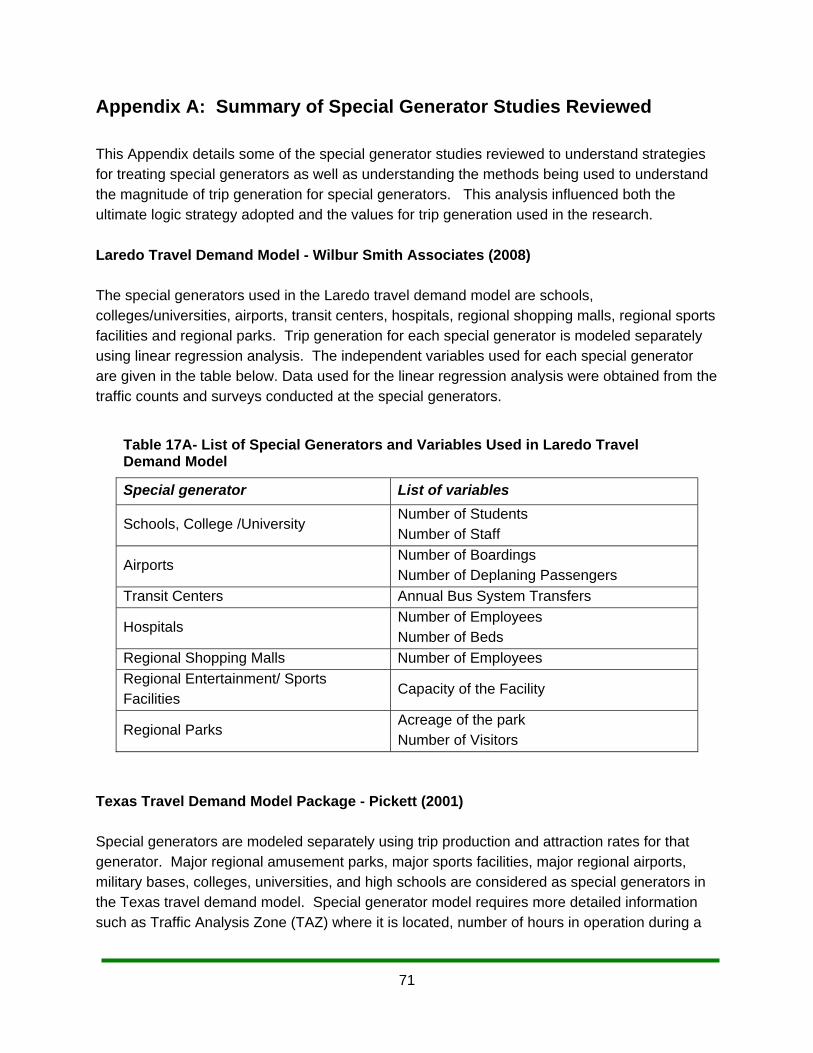
71

Appendix A: Summary of Special Generator Studies Reviewed

This Appendix details some of the special generator studies reviewed to understand strategies for treating special generators as well as understanding the methods being used to understand the magnitude of trip generation for special generators. This analysis influenced both the ultimate logic strategy adopted and the values for trip generation used in the research. Laredo Travel Demand Model - Wilbur Smith Associates (2008) The special generators used in the Laredo travel demand model are schools, colleges/universities, airports, transit centers, hospitals, regional shopping malls, regional sports facilities and regional parks. Trip generation for each special generator is modeled separately using linear regression analysis. The independent variables used for each special generator are given in the table below. Data used for the linear regression analysis were obtained from the traffic counts and surveys conducted at the special generators.

Table 17A- List of Special Generators and Variables Used in Laredo Travel Demand Model

Special generator List of variables

Schools, College /University Number of Students Number of Staff

Airports Number of Boardings Number of Deplaning Passengers

Transit Centers Annual Bus System Transfers

Hospitals Number of Employees Number of Beds

Regional Shopping Malls Number of Employees

Regional Entertainment/ Sports Facilities

Capacity of the Facility

Regional Parks Acreage of the park Number of Visitors

Texas Travel Demand Model Package - Pickett (2001) Special generators are modeled separately using trip production and attraction rates for that generator. Major regional amusement parks, major sports facilities, major regional airports, military bases, colleges, universities, and high schools are considered as special generators in the Texas travel demand model. Special generator model requires more detailed information such as Traffic Analysis Zone (TAZ) where it is located, number of hours in operation during a

72

normal weekday, number of work shifts, and number of employees per work shift. All the data required for calculating trip attraction rates are obtained by conducting surveys at the special generators. Following variables are used by the linear regression models for each special generator:

Table 18A- List of Special Generators and Variables Used in Texas Travel Demand Model

Special generators List of variables

Military Base Number of Employees

Schools, Colleges/Universities Number of Students Enrolled

Hospitals Number of Beds

Major Regional Airports Number of Flights/Day Number of Deplaning Passengers /Day

Lincoln MPO Travel Demand Model - Lima & Associates (2006) Lincoln travel demand model is used for the City of Lincoln in Lancaster County (Lincoln MPO). In this travel demand model, special generators are considered as land uses that do not generate or attract trips at the same rate as other land uses in the same land use category, hence they are assigned a unique trip rate. Nine special generators and the variables used to explain trip rates for these special generators used in Lincoln travel demand model are in the table below. Trip attraction for the internal non-residential land uses are estimated using a trip rate per unit (square feet, students, employees, etc.). These Non-Residential trip rates are obtained using “ITE Trip Generation Manual, 7th Edition”.

Table 19A - List of Special Generators and Variables Used in Lincoln MPO Travel Demand Model

Special generators List of variables (units)

Airports Number of Employees

Prison Number of Employees

Mall Area (1000 Sq.ft)

Medical Center Number of Employees

University Main Campus Number of Students

Heavy Industrial Area (acres)

Low Retail Area (1000 Sq.ft)

Low Office Area (1000 Sq.ft)

Low Service Area (1000 Sq.ft)

73

Dallas Fort-Worth Regional Travel Model (DFWRTM) (2006) In DFWRTM, special generators and the variables used to explain trip rates are shown in the table that follows.

Table 20A - List of Special Generators and Variables Used in DFWRTM


Regional Shopping Malls Number of Employees

University/Colleges Number of Employees

Hospitals Number of Employees

The trips attracted by special generators are computed by applying the trip attraction rates to the employment at respective sites and adding extra incremental trips associated with each category of special generator. The number of incremental trips for each special generator type is obtained by taking the difference of cross classification model generated trip rates and trip rates obtained from regional travel survey. Michigan Statewide Travel Demand Model - KJS Associates (1996) The Michigan Statewide Travel Demand Model is developed by KJS Associates for Michigan Department of Transportation (MDOT) and resides on the TransCAD 3.1 GIS/ Travel Demand Model Platform. Trip attraction equations were developed as a function of employment type by purpose. However, the trip attraction rates by employment type do not adequately reflect unique trip attractors (special generators). The special generators considered in this model are airports, tourist attractions, campgrounds, state parks, golf courses, marinas, motels, hospitals, shopping centers, colleges and universities. The trips attracted by special generators are computed by developing attraction rates using the following data sources: (1) ITE Trip Generation Manual, 5th Edition (all categories except bus terminals and tourist

attractions) and the ITE Trip Generation Manual, 3rd Edition (for community colleges only)

(2) Intercity Bus Study, Michigan DOT (for bus terminal category)

(3) Travel & Tourism Report, Michigan DOT (for tourist attractions) The variables used to explain the trip attraction by special generators are shown in the table that follows.

74

Table 21A - List of Special Generators and Variables Used in Michigan Statewide Travel Demand Model


Shopping Centers Area (Total Square Footage)

University/Colleges Number of Students

Hospitals Number of Beds

Tourist Attractions Attendance

Airports Registered Aircrafts and Operations

Marinas Number of Berths

Parks Acres

Whatcom County Travel Demand Model - Cambridge Systematics (2004) The Whatcom County Travel Demand Model was developed by Cambridge Systematics Inc. for Whatcom Council of Governments (WCOG) in Washington State. Airports, universities and colleges, casinos, harbors, hospitals and regional shopping centers are the special generators considered in this model. The trip attraction is captured in this model using the information on the variables of each special generator category shown in Table 22A. The differences of the estimates obtained from the regular model and ITE trip rates were added to the regular model by each trip purpose.

Table 22A - List of Special Generators and Variables Used in Whatcom County Travel Demand Model


Regional Shopping Centers Employees and Area (square feet)

University/Colleges Number of Students

Hospitals Employees

Airports Number of Flights

Trip Attraction Rates of Shopping Centers (SCs) in Northern New Castle County, Delaware - Kikuchi et al. (2004) Different from using the ITE Trip Generation Manual approach, this paper provides two possible approaches to calculate trip generation rates for shopping centers. These two approaches are based on the survey of the movement patterns (No. of people visiting and No. of vehicles).

75

(1) Macroscopic Approach

In this approach, trip attraction rate is a function of the physical features of individual shopping centers such as total parking space, total floor area, no. of stores and location of the shopping center (the ITE Trip Generation Manual does not consider these physical features). The influence of the total number of parking spaces, total floor area, and the number of stores on trip attraction rates is obtained by regression analysis. Data for linear regression analysis were obtained by conducting a traffic count survey for every 15 minute interval at various shopping centers on weekdays, Saturday and Sunday.

(2) Microscopic Approach

In this approach, importance is given to each store in the shopping center. The objective here is to determine weights for the trip attraction rates (TAR) of each store. The weighted sum of TARs of individual stores provides an overall TAR of the shopping center. TAR for different stores in a shopping center is obtained by conducting surveys for each store. A drawback of the microscopic model is its reliance on large volume of data for calculation of the TAR of individual stores and the weights. The number of people entering individual stores needs to be collected for different time periods.

A Comprehensive Planning and Design Manual for Park-and-Ride Facilities: Chapter 5 - Suburban Park-and-Ride Demand Estimation Techniques - Pillar (1997) Post Modeling Techniques This technique is used for individual park-and-ridepark-and-ride facilities and follows the traditional transportation modeling methodology. The steps involved in this modeling technique are as follows: (1) Identify the production ends (home zones) and attraction ends (work zones) of the potential

park-and-ridepark-and-ride site. (2) Identify the various characteristics of attraction ends such as parking cost, availability, traffic

congestion etc. (3) Determine total person trip interchange between the production zones and the attraction

zones by using modal splits from the regional travel model or other data sources. (4) Determine the proportion of trip interchange for Park and Carpool and Bus Park-and-Ride

users based on the characteristics of bus services and trip end density in attraction zones. (5) Estimate the number of parking spaces required at each site by developing trip interchange

tabulations based on the park-and-ride demand share.

76

Direct Regional Forecasting Techniques In this approach, park-and-ride trip is modeled as a chained trip directly within the regional modeling process. Park-and-ride is treated as an alternative mode in a mode choice model. Along with the decision to select park-and-ride versus the auto mode, commuters are assumed to decide which park-and-ride lot to choose depending on traffic congestion conditions. The park-and-ride lots immediately upstream of traffic congestion are expected to have high levels of demand. Site Level Forecasting based on Site and Service Characteristics This approach is based on the theory that site attributes and service characteristics define the attractiveness of the site to potential users. Therefore, park-and-ride demand is estimated based on the attributes of the park-and-ride location. This model assumes that attractiveness of one mode over another can be estimated by measuring the differences in site and service attributes between competing modes. Site specific demand is heavily influenced by a number of characteristics such as the location of lot, service characteristics and availability of competing lots and perceived convenience of the facility. A park-and-ride demand estimation study was done in the Greater Seattle metropolitan area for the King County Department of Metropolitan Services (Metro) on a bus transit network. The park-and-ride facilities were examined for their existing demand characteristics and the draw area associated with the patrons accessing the lot. A 1993 vehicle license plate survey was used as the basis for geocoding the residential location of vehicles observed in each of the 31 lots. Addresses for each observed parked vehicle were generated via a license plate search with the Washington Department of Motor Vehicles. The coordinates of each vehicle accessing individual lots were compared to the coordinates of the lot being used and then plotted on a common scale. The resulting service area demand sheds for each lot were compared to generate a catchment area shape. In all, this methodology is all about defining a service area (catchment area) for the park-and-ride facilities and then developing equations based on the lot attributes using multivariate regression analysis. Defining the market catchment area for park-and-ride The catchment area is defined based on the differences in parking costs, extent of transit network and perceived congestion in a region. Socio-economic data for the defined catchment area can be used to predict demand for the specific park-and-ride lot.

77

The shapes of the catchment area having 50 percent and 85 percent of the total observed users at each park-and-ride lot were considered. At the 85 percent user level, a parabolic shape nearly represents a catchment area of the lots. A circular pattern with a radial diameter of 2 to 2.5 miles, centered at the park-and-ride itself describes the average catchment area at the 50 percent demand level. Individual market areas are smaller than standard market areas because of features such as lakes and mountains. Using these catchment area shapes, overlaps and gaps between the park-and-ride facility services can be determined. This helps in mapping coverage zones of each facility and locating areas of service duplication and poor service. Identifying the site level characteristics affecting park-and-ride demand The variables that were considered to affect the demand for park-and-ride facilities at site level are as follows: Number of AM peak period express buses trips to central business district (CBD), number of AM peak period express buses trips to major employment centers other than CBD, ratio of out of pocket auto cost to transit costs, distance between park-and-ride lot and destination (CBD), total population within the 50 percent catchment area of lot, percentage of lower middle and lower income households within the service area of lot, the average best schedule transit time between park-and-ride lot and destination, peak traffic on adjacent roadway facility, number of home-based work trips between market area and destination, employment demand measure at the destination, relative measure of congestion between the park-and-ride lot and destination, age of park-and-ride lot, availability of priority treatments, safety characteristics of the lot, provision of passenger shelter and amenities, transit Information, parking costs at the destination and park-and-ride lot access attributes. Site level demand estimation The variables mentioned above were used to develop a planning tool to estimate the demand potential for park-and-ride facilities. The park-and-ride demand model is shown by following equation:- Demand = N + aAa1 + bBb1 + cCc1 ……+zZz1 where, N = Constant, incorporating a measure of the minimum lot size. A, B, C, Z = independent variables. a, b, c, z = model coefficients to be estimated using least square method. a1, b1, c1, z1 = variable exponents estimated using a least square method. This model cannot be directly transferred to other regions. The two options suggested by the authors to transfer the model to other regions are:

(1) Estimate a new model with local data to obtain the location-specific coefficients.

78

(2) Adjust the Seattle-specific equations developed in this study by a correction factor that compensates for the inherent differences between the region being studied and the Seattle metropolitan area.

Discount Superstore Trip Generation – Pearson et al. (2009) This study aims at developing trip rates for discount superstores such as Walmarts. To achieve this, a national discount superstore trip generation study was conducted by Texas Transportation Institute (TTI). A sample of 32 study sites was randomly selected from the 828 stores in original sample. Trip generation rates obtained using the survey data varied between individual superstores. Rates were developed using Gross Floor Area (GFA) as an independent variable. GFA data were obtained from an architecture firm. The results show that the rates obtained from the national study are higher than the ITE trip rates, but the differences are not statistically significant except for the Sunday daily rate. The study concludes that a high degree of variability and small numbers of observations in the ITE data are the reasons for this difference in trip rates. Transit Impact Fee Analysis: Technical Memorandum #2 Land Use and Trip Generation rates – The Duffey Company (2000) This study explores land uses that might be incorporated into an expanded Transit Impact Development Fee (TDIF) and describes trip generation rates associated with these land uses. Based on the preliminary assessment of potential transit trip generation for each land use, following land uses categories were identified as potential candidates for generating high number of transit trips: (1) Office

a. Professional/Business Office b. Professional Design Office

(2) Lodging a. Hotel/Motel

(3) Institutions a. Hospital, medical center b. Social/charitable service c. Child care facility d. Elementary/Secondary/Post-secondary school e. Churches or other religious institutions

(4) Community Facilities a. Community Club House b. Community Cultural center

(5) Assembly and Entertainment

79

a. Theatres b. Recreation Building c. Amusement Enterprise and parks/Citrus/Carnival d. Open air Stadium or arena

(6) Commercial (Retail)/ Personal Services a. Local Oriented retail b. Regional retail c. Bar d. Full-service restaurant e. Financial Services

(7) Manufacturing and Processing a. Light Manufacturing-assembly, packing, repair, processing b. Light Food Processing

The trip rates for the above land uses were obtained from the following sources:

(1) San Francisco Interim Transportation Impact Analysis Guidelines for Environmental Review, Interim Edition, January 2000, The Planning Department City and County of San Francisco.

(2) Trip Generation, 6th Edition, Institute of Transportation Engineers

(3) Citywide Travel Behavior Survey, Employees and Employers, May 1993, San Francisco Planning Department, San Francisco Public Utilities Commission, and San Francisco County Transportation Authority.

Quantifying Special Generator Ridership in Transit Analyses – Kurth et al. (1997) This proposes a four-step process for analyzing the impact of special generators on transit services in Denver area. The study area is “Gold Line”, a freight rail corridor between downtown Denver and Golden, Colorado. According to the authors, there are three types of special generators (1) Regular special generators: Special generators that produce trips on a regular, weekday

basis (e.g., airports, regional shopping centers, hospitals and schools)

(2) Periodic special generators: Special generators that do not produce trips on a regular weekday basis. (e.g., convention centers, stadia and arenas, fairs and festivals)

(3) Special generators: Those sites or activities that cannot be easily classified as regular or

periodic special generators.

80

This paper focuses on impact evaluation of periodic special generators. In the analysis process, generators having 500,000 attendees annually or 8,000 average individual event attendees were only considered. Events occurring at the same place were merged, if they did not meet the size criteria. Event attendance data were collected from the corresponding facilities (convention centers, stadia and arenas, etc.). Subsequently, the four-step process (with trip generation, trip distribution, mode choice, and transit assignment steps) was adopted and adapted for the purpose of the study. Direct Ridership Forecasting – Fehr & Peers Travel demand models do not consider changes in station-level land use and transit service characteristics. Direct ridership models are used to forecast transit patronage. Direct ridership models have been used to evaluate and compare various variables influencing transit patronage. They are used for light rail [Sacramento Regional Transit (RT) & Salt Lake City (TRAX)], commuter rail [Sonoma Martin Area Rail Transit (SMART)] and heavy rail [Bay Area Rapid Transit (BART)] forecasting. Direct ridership models use multivariate regression analysis based on the local land use data and data obtained from boarding and alighting counts at all stations. Thirty variables related to population and income, employment, cost of travel, station characteristics, transit service characteristics and comparative auto and transit accessibility were used to discover a combination of variables with a stronger correlation with ridership. For BART, ridership is a function of variables such as sum of population and employment within one-half mile of a station, population within station catchment area, frequency of peak period feeder buses, number of station parking spaces, and number of peak period trains. Sketch Model to Forecast Heavy Rail Ridership – Usvyat et al. (2009) The purpose of this paper is to study ridership potential for heavy rails by developing a model that considers variables related to the area surrounding the station. A multivariate linear regression model was created only for non-CBD stations using current ridership data collected for all 474 U.S heavy rail transit stations for the years 2004- 2006. The demographic information for both areas surrounding the stations and entire metropolitan area was obtained from the respective MPOs. The Model was developed using data from the following ten cities: Baltimore, Boston, Chicago, Cleveland, Los Angeles, Miami, New York (PATH train), Philadelphia, San Francisco, and Washington, DC. Exclusive regions around each station were used to avoid double counting of population and employment around station areas. Various independent variables related to station area demographics, station specific transportation attributes, corridor demographic characteristics and metro area demographics were tested in the model. The results show that employment and transit service characteristics are the best predictors of natural transit boardings.

81

Special Generator: Schools/Colleges/Universities For special generators such as schools, colleges and universities, student enrollments can best describes the trip generation. This data can be obtained from the following datasets: 2000 U.S Census data, Current Population Survey (CPS) and American Community Survey (ACS). (1) 2000 U.S Census Data:

School enrollment data were obtained from answers to a long-form questionnaire filled out by a sample of the population. People were classified as enrolled in school if they reported attending a "regular" public or private school, or college at any time between February 1, 2000, and the time of enumeration. The 2000 Census Summary File 3 data are available from the American Fact Finder on the internet (factfinder.census.gov).This data file gives annual enrollments and is available by gender, age, type of school and type of college. The 2000 Census Summary File 3 (SF 3) - sample data contains the following tables:

P36 Gender by school enrollment, by level of school, by type of school, for the population three years and over.

P38 Armed forces status by school enrollment, by educational attainment, by employment status for the population ages 16 to 19.

PCT23 Gender by school enrollment, by age, for the population three years and over.

PCT24 Gender by college or graduate school enrollment, by age, for the population 15 years and over.

(2) Current Population Survey (CPS) Data:

U.S Census Bureau conducts interviews for monthly Current Population Survey (CPS) and school enrollment data of households’ members three years old and over is obtained from CPS. This data gives annual enrollments for all the school and colleges in the United States. Data are available by gender, age, race, type of school and type of college. The data can be used to study the trip attraction of schools and colleges based on the variable number of students’ enrollment. The dataset is easily available from the following link: http://www.census.gov/population/www/socdemo/school.html (3) American Community Survey (ACS):

The American Community Survey (ACS) is a nationwide survey that began in January 2006 to replace the decennial census long form. ACS provides the annual (or multi-year average) estimates of selected social, economic, and housing characteristics of the population for many geographic areas and subpopulations. ACS gives school enrollment by age, gender, type of

82

school and type of college for the population 3 years and over. One year and three year estimates of American Community Survey are available from the following link: http://factfinder.census.gov/servlet/DatasetMainPageServlet?_program=ACS&_submenuId=datasets_1&_lang=en&_ts Special Generator: Airports (1) Passenger Boarding and All-Cargo Data

Federal Aviation Administration (FAA) extracts passenger (enplanement) and cargo data from the Air Carrier Activity Information System (ACAIS). These data are available only for Commercial Service Airports. Commercial Service Airports are publicly owned airports that have at least 2,500 passenger boardings each calendar year and receive scheduled passenger service. These airports are further classified into:

Primary Commercial Service Airports (that have more than 10000 passenger boardings per year)

Non primary commercial service airports (that have at least 2,500 and no more than 10,000 passenger boardings each year).

Passenger boarding and all-cargo data are collected for a full calendar year and determines entitlements for the next full fiscal year (i.e., calendar year 2007 data determines fiscal year 2009 entitlement funds). The dataset is easily available from the following link: http://www.faa.gov/airports/planning_capacity/passenger_allcargo_stats/passenger/

(2) FAA Terminal Area Forecast (TAF)

The Terminal Area Forecast (TAF) includes forecasts for active airports in the National Plan of Integrated Airport Systems (NPIAS). It is developed by FAA’s Forecasts and Performance Analysis Division, Office of Aviation Policy and Plans. The TAF contains historical and forecast data for enplanements and airport operations. This dataset includes information on FAA towered airports, federal-contracted towered airports, non-federal towered airports, and many non-towered airports. The 2009 database gives the enplanement forecast from 2010 to 2030. The 2009 model allows users to create their own forecast scenarios. The TAF database and TAF model is available online using the following link: http://aspm.faa.gov/main/taf.asp.This dataset helps in meeting the budget and planning needs of FAA and gives information for use by state and local authorities, the aviation industry, and the public. Special Generator: Hospitals The American Hospital Association (AHA) annual survey is an online survey taken by more than 6500 AHA registered hospitals throughout the United States. This database is used for market

83

research and health care industry analysis on hospitals. The database captures information such as facilities provided, hospital utilization, number of beds, admissions, etc., on each hospital. The number of beds best describes the trip generation for hospitals. This dataset is available at state and regional geographic level. This dataset is not available online and can be purchased in the form of CD and book. More information can be obtained using the following link: http://www.ahadata.com/ahadata/html/AHASurvey.html

84

Appendix References

Ammi, S. “Trip Generation Manual. San Diego Municipal Code.”, Last Modified May 2003.

http://www.sandiego.gov/planning/pdf/tripmanual.pdf.

Baik, H., A. A. Trani, N. Hinze, H. Swingle, S. Ashiabor, and A. Seshadri. “Forecasting Model for Air Taxi, Commercial Airline, and Automobile Demand in the United States.” Transportation Research Record: Journal of the Transportation Research Board 2052, (2008): 9–20.

Carter, M. “Transit and Traffic Analysis.” Transportation Research Board Special Report 206 (1985): 152-157.

Center for Urban Transportation Studies, University of Wisconsin-Milwaukee. “Transit Route Location and Analysis, Understanding Transit: Basic Course Material on Public Transportation.” Last Modified July 2006. http://www4.uwm.edu/cuts/utp/

The Duffey Company and Nelson/Nygaard Consulting Associates, “Transit Impact Fee Analysis: Technical Memorandum #2 Land Use and Trip Generation Rates.” Prepared for the San Francisco Planning Department, San Francisco, California, September 2000.

Florida Department of Transportation, Tallahassee. “T-BEST (Transit Boardings Estimation and Simulation Tool).” Last Modified 2009, www.tbest.org

Hull, Edwin., Edwin Hull Associates. “Application of a Park-and-Ride Forecasting Procedure in the Greater Vancouver Transportation Model”, Presented in the 13th Annual International EMME/2 Users’ Group Conference, Houston, Texas, October 1998.

Kikuchi, S., M. Felsen, S. Mangalpally, and A. Gupta. “Trip Attraction Rates of Shopping Centers in Northern New Castle County, Delaware. Prepared for the Delaware Department of Transportation, July 2004.

Kittelson & Associates, Inc. “A Guidebook for Developing a Transit Performance-Measurement System.” TCRP Report 88 ( 2003).

Kurth, David L., B. V. Meter, S. Myung, and M. C. Shaefer. “Quantifying Special Generator Ridership in Transit Analysis.” Proceedings of the Sixth TRB Conference on the Application of Transportation Planning Methods, Dearborn, Michigan, May 1997.

Lima & Associates. “Lincoln MPO Travel Demand Model Documentation” Prepared for the Lincoln Metropolitan Planning Organization, January 2006.

85

LSA Associates, Inc. “Weekend Travel Demand Model: Technical Memorandum #9 - Special Generators for the Weekend Model.” Prepared for the Southern California Association of Governments, June 2008.

McDonnell, S., Ferreira, S., and Convery, F. “Impact of Bus Priority Attributes on Catchment Area Residents in Dublin, Ireland.” Journal of Public Transportation, 9, no. 3. (2006): 137–62.

Murray, A., Davis, R., Stimson, R., and Ferreira, L. “Public Transport Access.” Transportation Research D 3 (1998): 319-28.

Murray, A. “Strategic Analysis of Public Transport Coverage.” Socioeconomic Planning Sciences 35 (2001): 175-188.

Neilson, G. K. and Fowler, W. K. “Relationship Between Transit Ridership and Walking Distances in a Low Density Florida Retirement Area.” Highway Research Record 403 (1972): 26–34.

Parsons Brinckerhoff. “WACOG Connector Program Transit Feasibility and Implementation Plan, Task 1: Transit Demand Model Summary.” Prepared for the Western Arizona Councils of Governments (WACOG), September 2000.

Pascoe, R. “Updating Demographics Using Parcel Data for Transit Corridor Analyses.” Presented at National Center for Transit Research (NCTR’s) GIS in Transit Conference, Tampa, Florida, 2007.

Pearson, David F., B. S. Bochner, P. Ellis, M. I.Ojah. “Discount Superstore Trip Generation.” Institute of Transportation Engineers (ITE) Journal (2009).

Pickett, W. Kirby. “Traffic Data and Analysis Manual: Chapter 2 (Section 2) - Texas Travel Demand Model Package.” Last Modified September 1, 2001, http://onlinemanuals.txdot.gov/txdotmanuals/tda/ urban_travel_demand_forecasting.htm

Pillar, Robert S., Parsons, Brinckeroff, Quade, & Douglas, Inc. “A Comprehensive Planning and Design Manual for Park-and-Ride Facilities” Suburban Park-and-Ride Demand Estimation Techniques. October 1997.

Rana, Tejsingh A. "Enhancement of Predictive Capability of Transit Boardings Estimation and Simulation Tool (TBEST) Using Parcel Data: An Exploratory Analysis.” Department of Civil and Environmental Engineering, University of South Florida.( 2010).

Reese, M. “ A GIS Analysis of the Bus Rapid Transit System in Curitiba, Brazil.” Student project for course PLAN 512 GIS for Planners, University of Virginia, Fall 2007. http://www.arch.virginia.edu/~dlp/Courses/P512F07/CuritibaGIS_presentationopt.pdf_

86

Sullivan, S., O and J. Morrall. “Walking Distances To and From Light-Rail Transit Stations.” Transportation Research Record 1538 (1996): 19–26

Transportation Department of North Central Texas Council of Governments (NCTCOG).

“Dallas-Fort Worth Regional Travel Model Description.” June 2006. U.S. Census Bureau. “School Enrollment Data. Current Population Survey.” Last Modified

October 2007, http://www.census.gov/population/www/socdemo/school.html. U.S. Department of Commerce, Bureau of Transportation Statistics. “T-100 International

Segment (All Carriers) Database.” Last Modified December 2008, www.transtats.bts.gov/Fields.asp?Table_ID=261.

U.S. Department of Transportation. “Passenger Boarding Statistics, Federal Aviation Adminstration.” Last Modified September 26, 2008, http://www.faa.gov/airports/planning_capacity/passenger_allcargo_stats/passenger/.

Usvyat, Len, Meckel, L., and Dicarlantonio, M. “Sketch Model to Forecast Heavy Rail Ridership.” Proceedings from the 12th TRB National Transportation Planning Applications Conference, Houston, Texas, May 2009.

Wilbur Smith Associates. “Laredo Metropolitan Transportation Plan 2005- 2030: Chapter 3 –

Demographics and Travel Demand Model.” Prepared for the Laredo Metropolitan Planning Organization, January 2008.

Xuehao, C., Polzin, S., Pendyala, R., Siddiqui, N., and Ubaka, I. “A Framework of Modeling and Forecasting Stop-Level Transit Patronage.” Presented at the 86th Transportation Research Board Annual Meeting, Washington, D.C., 2007.

Zhao, F., Chow, L.-F., Li, M.-T., Ubaka, I., Gan, A. “Forecasting Transit Walk Accessibility: Regression Model Alternative to the Buffer Method.” Transportation Research Record 1835, (2003): 34–41.

TBEST Model Enhancements - Parcel Level …...TBEST Model Enhancements—Parcel Level Demographic...

Documents

Transcript of TBEST Model Enhancements - Parcel Level …...TBEST Model Enhancements—Parcel Level Demographic...