Tax˜Competition˜and˜Spatial˜Competition:˜ The˜Effect˜of ...
41
Tax Competition and Spatial Competition: The Effect of Falling Transport Costs and Electronic Commerce Jonathan H. Hamilton Department of Economics Warrington College of Business Administration University of Florida Jacques-François Thisse Center for Operations Research and Econometrics Université Catholique de Louvain September 2002 We thank Mark Scanlan for excellent programming assistance. The first author thanks the Warrington College of Business Administration, ICAIR, and the University of Florida CIBER for financial support for this research. The second author thanks ICAIR for financial support for this research. Any remaining errors are our sole responsibility.
Transcript of Tax˜Competition˜and˜Spatial˜Competition:˜ The˜Effect˜of ...
����
�Tax�Competition�and�Spatial�Competition:�
The�Effect�of�Falling�Transport�Costs��and�Electronic�Commerce�
�
Jonathan�H.�Hamilton�Department�of�Economics�
Warrington�College�of�Business�Administration�University�of�Florida�
�Jacques-François�Thisse�
Center�for�Operations�Research�and�Econometrics�Université�Catholique�de�Louvain�
�September�2002�
���������������������We�thank�Mark�Scanlan�for�excellent�programming�assistance.��The�first�author�thanks�the�Warrington�College�of�Business�Administration,�ICAIR,�and�the�University�of�Florida�CIBER�for�financial�support�for�this�research.��The�second�author�thanks�ICAIR�for�financial�support�for�this�research.��Any�remaining�errors�are�our�sole�responsibility.�

� 2
Abstract�
� We�study�the�effect�of�the�growth�in�electronic�commerce�on�retail�sales�taxes�
using�the�logit�model�of�product�differentiation.��Competing�jurisdictions�choose�tax�rates�
on�retail�businesses�in�their�own�jurisdictions�and�then�firms�choose�prices.��We�solve�
numerically�for�the�subgame�perfect�Nash�equilibria�of�these�games.�
� We�consider�two�different�tax�structures,�which�differ�in�the�treatment�of�sales�by�
businesses�in�one�jurisdiction�to�consumers�in�another�jurisdiction.��The�first�assumes�
complete�evasion�of�use�taxes�(consumers�who�buy�outside�their�home�jurisdiction�escape�
all�sales�taxes),�which�is�close�to�the�status�quo�in�the�U.S.��The�second�assumes�zero�use�
tax�evasion,�which�is�close�to�the�status�quo�in�the�EU.�
� We�find�that�both�tax�rates�and�tax�revenue�fall�sharply�in�a�switch�from�zero�to�
full�use�tax�evasion.��The�effect�is�greater�for�lower�costs�of�cross-border�shopping.��We�
also�discuss�some�differences�in�comparative�statics�between�the�two�tax�regimes.�

1.��Introduction�
� State�and�local�governments�in�the�U.S.�collect�a�significant�fraction�of�their�total�
tax�revenue�through�retail�sales�taxes.��This�tax�base�faces�threats�of�erosion�from�several�
sources:��declines�in�the�share�of�sales�of�taxable�goods�in�national�income;�the�growing�
importance�of�mail-order�sales;�and�the�recent�development�of�electronic�commerce.��The�
first�of�these�causes�has�led�some�states�to�attempt�to�expand�sales�taxes�from�goods�to�
services.��The�latter�two�sources�of�erosion�have�a�similar�cause—changes�in�
technology—shipping�goods�directly�to�consumers�has�become�less�costly�due�to�declines�
in�transportation�costs,�and�possibly�more�importantly,�declines�in�handling�and�
processing�costs.�
State�governments�which�levy�sales�taxes�also�levy�use�taxes,�so�that�residents�of�
the�jurisdiction�are�liable�for�an�equivalent�tax�in�their�place�of�residence�on�goods�
purchased�elsewhere.��A�1967�Supreme�Court�decision�and�a�later�affirmation�[National�
Bellas�Hess,�386�U.S.�753,�1967;�Quill,�504�U.S.�298,�1992]�require�that��sellers�have�
nexus�in�a�jurisdiction�in�order�for�it�to�be�responsible�for�collecting�sales�or�use�taxes�for�
that�jurisdiction.1�Congress�has�repeatedly�declined�to�overturn�the�Court’s�decision.��As�
a�result,�the�collection�experience�for�use�taxes�is�so�abysmal�that�one�can�almost�ignore�
them.��The�recent�moratorium�on�Internet�taxes�extends�this�treatment�of�mail�order�sales�
to�Internet�sales�by�probiting�new�tax�regulations�specifically�targeting�Internet�sales.�
While�mail-order�sales�to�consumers�have�grown�since�the�1960s,�few�would�
assert�that�the�favorable�tax�treatment�is�the�only�cause.��Similarly,�the�tax�treatment�
explains�only�some�of�the�recent�growth�of�electronic�commerce�[Goolsbee,�2000].��
Rapid�technological�advances�in�logistics�and�falling�transportation�costs�for�quick�

� 2
delivery�of�small�packages�have�also�made�mail-order�or�Internet�shopping�simpler�and�
easier.��The�ability�of�mail-order�firms�to�hold�more�varieties�in�inventory�than�
conventional�retailers�has�probably�also�contributed�to�growth�of�this�sector.2�
State�and�local�government�officials�are�rightly�concerned�about�the�future�of�the�
sales�tax�base�unless�they�can�require�sellers�to�assist�them�in�collecting�use�taxes.��Many�
conventional�(“bricks-and-mortar’)�retailers�are�also�concerned�about�the�tax�
disadvantage�they�face�in�competing�with�Internet�retailers.��In�addition�to�use�tax�
evasion,�mail-order�and�Internet�retailers�are�considerably�more�mobile�and�can�seek�out�
locations�with�lower�overall�business�taxes.���Declines�in�the�costs�to�consumers�of��
buying�outside�their�residence�jurisdictions�increase�the�intensity�of�tax�competition�
among�jurisdictions.��They�also�make�the�intensity�of�price�competition�among�firms�
fiercer�in�many�monopolistic�competition�models.�
� We�model�a�two-stage�game�of�tax�competition.��First,�each�jurisdiction�
simultaneously�chooses�its�tax�rate�to�maximize�a�composite�objective�function�
(including�revenue,�resident�welfare,�and�profits�of�resident�firms).��These�tax�rates�then�
influence�demand�and�costs�for�retailers�based�in�the�different�jurisdictions.��Retailers�
simultaneously�choose�prices�given�the�set�of�tax�rates�facing�all�active�firms.��We�solve�
numerically�for�subgame-perfect�Nash�equilibria�of�this�two-stage�game�under�different�
tax�regimes.�
� Section�2�discusses�the�tax�issues�and�some�previous�literature.��Section�3�presents�
the�basic�model.��Section�4�describes�the�price�equilibrium�and�Section�5�describes�the�tax�
equilibrium.��Section�6�presents�our�main�simulation�results.��Section�7�contains�our�
conclusions�and�discusses�goals�for�further�research.�
�

� 3
2.��The�Tax�Issues�
There�are�many�models�of�interjurisdictional�competition�in�public�economics.��
The�structure�of�local�government�finance�in�the�U.S.�led�to�an�initial�focus�on�property�
tax�competition.��The�Tiebout�model�[1956]�has�been�a�common�starting�point�to�study�
residential�property�taxes.��In�choosing�where�to�reside,�households�select�a�combination�
of�property�taxes�and�public�goods.��With�a�large�number�of�local�governments�in�a�
metropolitan�labor�market,�jurisdictions�offer�both�the�appropriate�level�of�services�for�
their�residents�and�provide�these�services�efficiently.��What�generates�efficient�outcomes�
in�the�simpler�forms�of�Tiebout�model�is�the�tight�connection�between�paying�taxes�and�
receiving�services.��The�efficiency�holds�when�only�residential�land�values�are�taxed.��
Since�non-residential�real�estate�and�residential�structures�also�face�local�property�taxes,�
the�property�tax�does�have�some�distortionary�effects.��
For�retail�sales�taxes,�the�link�between�paying�taxes�and�receiving�services�breaks�
down.��A�jurisdiction�with�a�low�tax�rate�can�attract�shoppers�from�other�jurisdictions�
without�the�burden�of�having�to�provide�any�government�services�to�them.3��Because�of�
this,�tax�competition�may�lead�to�underprovision�of�public�services�since�the�perceived�
marginal�cost�of�public�funds�may�be�quite�high.�
One�issue�we�need�to�explore�as�part�of�this�study�is�the�incidence�of�differential�
sales�taxes�in�oligopoly.��There�has�been�some�previous�work�in�this�area.��Braid�[1987]�
studies�the�incidence�of�sales�taxes�in�a�spatial�oligopoly.��Consumers�buy�from�the�store�
with�the�lowest�price�plus�transport�cost.��Braid�examines�the�effect�of�a�single�
jurisdiction�with�one�or�more�stores�raising�its�tax�rate,�but�he�does�not�examine�the�
equilibrium�tax�rates�for�several�jurisdictions.�Trandel�[1992]�is�another�paper�along�

� 4
similar�lines.��Other�papers�such�as�Braid�[1993]�and�Trandel�[1994]�study�equilibrium�
tax�rates,�but�they�confine�themselves�to�models�with�a�single�store�per�district.��A�
common�feature�in�the�literature�is�that�there�is�complete�market�segmentation—each�
store’s�customers�are�a�distinct�segment�of�the�market.��Given�that�only�some�consumers�
shop�via�the�Internet,�it�seems�important�to�study�models�with�imperfect�customer�
segmentation.�
There�is�another�literature�studying�tax�competition�when�firms�use�marginal�cost�
pricing,�including�Kanbur�and�Keen�[1993].��Given�the�importance�of�product�
differentiation�in�many�mail-order�product�lines,�it�seems�more�appropriate�to�study�
price-setting�firms�even�at�the�cost�of�more�complexity.�
� Currently,�only�retail�stores�collect�sales�taxes�for�their�jurisdictions.��Mail-order�
and�Internet�retailers�collect�sales�taxes�only�for�shipments�within�the�same�jurisdictions.�
Growth�in�sales�through�other�channels�could�lead�jurisdictions�to�replace�sales�taxes�with�
other�types�of�taxes�on�producers�and�distributors.��In�effect,�these�new�taxes�would�be�
taxes�based�on�the�origin�principle�(the�tax�rate�in�the�seller’s�jurisdiction�would�apply�to�
transactions).���
� For�now,�we�focus�on�the�effects�of�eliminating�use�tax�evasion.��We�thus�
compare:�
1)� the�current�U.S.�tax�system�with�100%�use�tax�evasion,�and�
2)� sales�taxes�based�on�the�destination�principle,�which�applies�for�intra-EU��
transactions.4�
� �

� 5
3.��The�Model�
Since�consumers�in�the�same�jurisdiction�patronize�stores�in�several�jurisdictions�
and�each�store’s�customers�may�reside�in�many�different�jurisdictions,�it�seems�useful�to�
examine�models�with�incomplete�market�segmentation.��The�most�workable�of�these�
models�is�the�logit�model�of�product�differentiation�which�is�studied�in�detail�in�
Anderson,�de�Palma,�and�Thisse�[1992].���Heterogeneity�among�consumers�in�this�model�
enables�stores�to�have�overlapping�market�areas�even�with�perfect�information�about�
prices�on�the�part�of�consumers.��Such�a�model�seems�quite�useful�to�study�consumer�
behavior�in�shopping�through�different�channels�such�as�retail�shops,�mail�order,�and�
electronic�commerce�Web�sites.�
� We�model�demand�for�an�individual�product�or�product�group�using�a�well-known�
model�of�discrete�choice�by�consumers�among�differentiated�products.��Each�consumer�
chooses�among�all�available�products,�as�well�as�an�outside�option�(buying�no�variety�of�
output�in�this�particular�industry).��The�total�population�of�consumers�is�normalized�to�
one,�with�γ�living�in�jurisdiction�1�and�1�−�γ�living�in�jurisdiction�2.�There�are�N1�firms�in�
jurisdiction�1�and�N2�firms�in�jurisdiction�2.��We�first�study�a�tax�system�in�which�each�
jurisdiction�levies�an�ad�valorem�sales�tax,�and�there�is�100%�use�tax�evasion—no�
consumers�pay�sales�tax�(to�either�jurisdiction)�on�purchases�outside�their�residence�
jurisdiction.5�
� We�first�write�the�demand�for�firm�i�as�the�sum�of�two�components:��from�
consumers�in�its�“home”�jurisdiction�and�from�consumers�in�the�“foreign”�jurisdiction,�
or:� Di�=�γHi�+�(1�−�γ)Fi� where� �1i
1i
i
)1(pexp
H∆
µ
τ+−
= �

� 6
µ
τ+−−+
µ
τ+−=∆
)1(pexp)1N(
)1(pexp 11
11i
1i �
µ
+
µ
δ−−+ 022
Vexp
pexpN �
� �2i
i
i
pexp
F∆
µ
δ−−
= �
and� ∆i2�=� i 11
p pexp (N 1)exp
− − δ − − δ + − µ µ
µ
+
µ
τ+−+ 0222
Vexp
)1(pexpN .�
In�words,�Hi(pi,�p1,�p2)�equals�the�probability�that�a�consumer�residing�in�
jurisdiction�1�buys�from�firm�i�in�jurisdiction�1�when�firm�i�charges�pi,�the�remaining�
firms�in�jurisdiction�1�charge�p1,�and�all�firms�in�jurisdiction�2�charge�p2.��When�the�
consumer�buys�from�a�store�in�her�home�jurisdiction,�the�after-tax�price�equals�pi(1+τ1).��
When�buying�from�a�store�in�the�other�jurisdiction,�the�after-tax�price�equals�p2,�but�the�
consumer�incurs�an�additional�cost�of�δ�in�making�a�purchase�outside�the�jurisdiction.��In�
accord�with�some�casual�observation,�we�assume�that�firms�are�unable�to�discriminate�in�
price�between�resident�and�non-resident�consumers.��In�other�words,�firm�i�charges�the�
same�mill�price�pi�regardless�of�where�her�customers�are�located,�so�that�the�hassle�cost�of�
δ�is�paid�by�the�consumer.��New�technology�reduces�δ�and�the�comparative�statics�of�
changes�in�δ�are�a�major�focus�of�our�work�here.�
� Similarly,�Fi(pi,�p1,�p2)�equals�the�probability�that�a�consumer�residing�in�
jurisdiction�2�buys�from�firm�i�in�jurisdiction�1�when�firm�i�charges�pi,�the�remaining�
firms�in�jurisdiction�1�charge�p1,�and�all�firms�in�jurisdiction�2�charge�p2.�
� Finally,�the�term�V0�stands�for�the�utility�of�the�outside�option,�whereas�µ�is�a�
scale�parameter�which�reflects�the�responsiveness�of�a�consumer�to�differences�in�the�
“observable�utility”�among�the�different�options�(including�the�outside�one).�

� 7
Let�firm�j�be�a�representative�firm�in�jurisdiction�2.��Its�demand�equals:�
� Dj�=�γFj�+�(1�-�γ)Hj� where�2j
2j
j
)1(pexp
H∆
µ
τ+−
= �
µ
τ+−−+
µ
δ−−=∆
)1(pexp)1N(
pexpN 22
21
12j
µ
+
µ
τ+−+ o2j V
exp)1(p
exp �
1j
j
j
pexp
F∆
µ
δ−−
= � and�
∆j1�=�N1�exp�
µ
δ−−−+
µ
τ+− 22
11 pexp)1N(
)1(p+�exp
µ
+
µ
δ−−oj V
expp
.�
4.��The�Price�Equilibrium�
We�consider�only�quasi-symmetric�equilibria�in�which�all�firms�in�jurisdiction�1�
charge�the�same�price�and�all�firms�in�jurisdiction�2�charge�the�same�price.��We�write�the�
demand�facing�a�firm�in�jurisdiction�1�as�a�function�of�the�triple�(pi,�p1,�p2)�in�order�to�
distinguish�between�its�own�price�and�the�price�of�its�rivals�in�the�same�jurisdiction�in�
order�to�derive�the�demand�derivatives�we�need�to�find�the�Nash�equilibrium�in�prices.�
� Since�pi�and�pj�are�producer�prices,�the�profit�functions�for�the�representative�firms�
are:� � � Πi(pi,�p1,�p2)�=�(pi�-�c)Di(pi,�p1,�p2)�
and� Πj(pi,�p1,�p2)�=�(pj�-�c)Dj(pj,�p1,�p2),�
where�c�is�marginal�cost�(which�we�assume�to�be�identical�across�all�firms�and�for�all�
types�of�sales).��We�ignore�any�fixed�costs,�since�our�analysis�considers�exogenous�
numbers�of�firms.�
� The�first-order�conditions�for�profit�maximization�are:�

� 8
� �i
i
p∂Π∂
=�Di�+�(pi�-�c)�i
i
p
D
∂∂
�=�0�
and�j
j
p∂Π∂
=�Dj�+�(pj�-�c)�j
j
p
D
∂∂
=�0,�
where�the�demand�derivatives�equal:�
�
∂∂
γ−+
∂∂
γ=∂∂
i
i
i
i
i
i
p
F)1(
p
H
p
D�
� �
µτ+
+µτ+−
γ= 2i
1i
1 )H()1(
H)1(
µ
+µ
−γ−+ 2ii )F(
1F
1)1( �
and�j
j
j
j
j
j
p
H)1(
p
F
p
D
∂∂
γ−+∂∂
γ=∂∂
�
� �
µ
+µ
−γ−+
µτ++
µτ+−γ= 2
jj2
j2
j2 )F(
1F
1)1()H(
)1(H
)1(.�
With�a�single�market,�existence�of�a�pure�strategy�Nash�equilibrium�in�prices�is�
guaranteed�(see�Anderson,�de�Palma,�and�Thisse�1992).��Because�the�demand�functions�
are�the�sum�of�two�logits,�their�proof�cannot�be�applied�directly.6��However,�a�quasi-
symmetric�equilibrium�can�be�guaranteed�to�exist�for�the�levels�of�tax�rates�we�observe.�
�Proposition�1:��If�max{τ1,�τ2}�<� τ̂ ,�min{N1,�N2}�≥�2,�and�µ�>�0,�there�exists�a�Nash�
equilibrium�in�prices�in�which�all�firms�in�each�jurisdiction�charge�a�single�price.�
Proof:��See�Appendix�A.�
�� Closed-form�solutions�for�these�equilibrium�prices�are�unavailable,�even�with�N1�
=�N2�and�τ1�=�τ2�(except�with�zero�tax�rates).��While�specific�taxes�are�not�a�common�way�

� 9
to�assess�sales�taxes,�it�is�instructive�to�consider�them�because�an�analytic�solution�is�
available�in�the�symmetric�case.�
�Proposition�2:��Let�t1�=�t2�=�t�be�the�specific�sales�tax�assessed�in�both�jurisdictions.��For�
N1�=�N2�=�N,�the�equilibrium�price�charged�by�all�firms�is:�
� p*(N,�t,�δ)�=�c�+�ΓµN
� �
where� ( ) ( )22 )exp(1
)exp(N1N
)exp(1
)exp(N1N
β+β+−+
β−+β−+−=Γ �and�β�=�
µ−δ t
.�
An�increase�in�δ�or�a�decrease�in�t�have�the�same�effect�on�p*,�and�*p∂
∂δ>�0�if��δ�>�t��
(and�<�0�if��δ�<�t).�
Proof:��Firm�i�in�jurisdiction�1�has�the�demand�curve:�
i 1
i
i 1 1 1 21 2
p texp
Xp t p t p
exp (N 1)exp N exp
− − µ =
− − − − − − δ + − + µ µ µ
�
�
� +�
i
i 1 2 21 2
pexp
p p p texp (N 1)exp N exp
− − δ µ
− − δ − − δ − − + − + µ µ µ
�=�F1
H1 + �
�
� where� 1 i 2 i 11 2
p p p p tH 1 (N 1)exp N exp
− + − − δ + + = + − + µ µ
�
� and�� 1 i 2 2 i1 2
p p p t pF 1 (N 1)exp N exp
− + − − + + δ = + − + µ µ
.�
Profit�for�firm�i�equals�Πi�=�(Pi�−c)Di.��To�obtain�firm�i’s�best�reply,��
� i ii i
i i
XX (p c)
p p
∂Π ∂= + −
∂ ∂=�0�or�
�

� 10
�F
1
H
1 + 1 1 ii 2
(N 1) p p1(p c) exp
H
− − + −+ − µ µ 2 2 i 1N p p texp
− − δ + + + µ µ
�
�
� � � � 1 1 i 2 2 2 i2
(N 1) p p N p t p1exp exp
F
− − + − − + + δ − + µ µ µ µ =�0.�
�At�the�symmetric�solution�when�t1�=�t2�=�t�and�N1�=�N2�=�N,�pi�=�p1�=�p2�=�p:��
� � �
µ−δ+
+
µδ−+ t
exp1N
1
texp1N
1�
�
� � � �2 2 2
t tN 1 Nexp N 1 Nexp
(p c)
N t t1 exp 1 exp
− δ δ − − + − + µ µ − − + µ − δ δ − + + µ µ
�=�0�
�
or�
2 2
(p c) 1
N t tN 1 Nexp N 1 Nexp
t t1 exp 1 exp
− =µ − δ δ − − + − + µ µ +
− δ δ − + + µ µ
�=�Γ1
�
�
Let�β�=�µ−δ t
;�then� ( ) ( )22 )exp(1
)exp(N1N
)exp(1
)exp(N1N
β+β+−+
β−+β−+−=Γ .�
��
Differentiating�p*�with�respect�to�β,�we�obtain�*
2
p N∂ −µ ∂Γ=∂β ∂βΓ
.��Since��
β+−ββ−=
β∂Γ∂
3)]exp(1[
1)exp()exp(2 ,�
*p∂∂β
has�the�same�sign�as�exp(β)�–�1.��Thus,�*p∂
∂β>�0�if�
δ�>�t.� � � � � � � � � � � QED�
�
),( 21 ττ

� 11
The�reversal�of�the�effect�of�a�tax�rate�increase�as�δ�>�t�changes�sign�may�seem�
surprising.��The�intuition�is�straightforward.��When�δ�>�t,�a�consumer�buys�more�in�his�
jurisdiction;�on�the�other�hand,�when�δ�<�t�he�buys�more�from�the�distant�jurisdiction.�
The�analysis�of�the�price�equilibrium�under�ad�valorem�taxes�requires�simulation�
analysis�because�there�do�not�exist�closed-form�solutions�for�equilibrium�prices.��Table�1�
displays�some�illustrative�simulation�results�for�equilibrium�prices�under�ad�valorem�
taxes.���
Under�the�no-use-tax-evasion�regime�(NUTE),�symmetric�increases�in�taxes�find�
about�one�quarter�to�one-third�of�a�tax�increase�being�absorbed�by�the�firms:�
0.01670.2502
0.05(1.3253)= � for�µ�=�0.3��
and��0.0268
0.35060.05(1.5287)
= � for�µ�=�0.5.�
Increases�in�δ�result�in�only�small�changes�to�these�absorption�rates.7��Asymmetric�tax�
increases�(moving�from�τ1�=�τ2�=�0.10�to�τ1�=�0.15�and�τ2�=�0.10,�for�example)�result�in�
smaller�price�changes�for�firms�in�both�jurisdictions,�with�the�price�change�for�the�firms�
more�directly�affected�being�about�150%�of�the�price�change�for�the�firms�in�the�
jurisdiction�whose�tax�rate�remains�constant.�
� Under�the�use-tax-evasion�regime�(UTE),�for�symmetric�5%�increases�in�tax�rates,�
price�changes�absorb�one-sixth�to�one-fifth�of�the�tax.��For�asymmetric�changes�in�tax�
rates,�the�directly�affected�firms�absorb�about�the�same�fraction�of�the�tax�as�under�
NUTE,�but�the�firms�in�the�jurisdiction�with�unchanged�tax�rates�change�price�hardly�at�
all.��More�importantly,�these�firms�may�raise�or�lower�price�when�rival�firms�in�the�other�
jurisdiction�face�a�tax�increase.�

� 12
5.��The�Tax�Equilibrium�
We�take�a�flexible�approach�to�the�question�of�each�jurisdiction’s�objective�
function�and�assume�that�it�consist�of�several�items.��For�simplicity,�we�restrict�ourselves�
to�weighted�sums�of�these�factors�as�the�objectives.��The�components�are:�
� 1)� tax�revenue�
� 2)� consumer�surplus�
and�� 3)� profits.�
Clearly,�tax�revenue�matters�for�two�reasons:��financing�purchases�of�public�goods�
and�services,�and�allowing�reductions�in�other�tax�rates.��Conventional�optimal�tax�
considerations�would�suggest�that�a�local�jurisdiction�would�prefer�not�to�rely�on�a�single�
tax�base,�but�to�tax�as�many�different�bases�as�possible�at�lower�rates.��Counting�revenue�
and�consumer�surplus�separately�means�effectively�that�we�assume�that�consumers’�utility�
is�additively�separable�in�public�and�private�goods�and�also�additively�separable�between�
the�goods�in�the�monopolistically�competitive�sector�and�all�other�goods�(which�are�the�
outside�option).�
� Local�governments�value�the�profitability�of�their�resident�firms�for�several�
reasons.��Among�them�are�revenues�from�taxes�on�business�profits,�incomes�to�local�
owners,�and�economic�rents�to�local�factors�which�depend�on�business�profits.8��
� Formally,�jurisdiction�1’s�tax�revenue�is�R1�=�τ1p1(γN1Hi)�since�taxes�are�only�
collected�on�sales�by�resident�firms�to�resident�consumers.9��Each�jurisdiction�only�
considers�the�surplus�of�its�own�residents�in�setting�its�ad�valorem�tax�rate.��From�
Anderson,�de�Palma,�and�Thisse�[1992,�p.�61],�consumer�surplus�is:�

� 13
S1�=�
µ
µ ∑n
1iu
expln ��
where�ui�equals�minus�the�full�price�of�alternative�i�(-�p1(1+τ1)�or�–p2�-�δ).�
� Consumers�in�jurisdiction�1�choose�among�N1�firms�in�jurisdiction�1�and�N2�firms�
in�jurisdiction�2.��Thus,�
� S1�=�
µ
+
µ
+
µ
µ 0122
111
Vexp
uexpN
uexpNln �
� � � where�u11�=�-p1(1+τ1)���and�u12�=�-p2�-δ.�
Similarly,�S2�=�
µ
+
µ
+
µ
µ 0211
222
Vexp
uexpN
uexpNln �
� � � where�u22�=�-p2(1+τ2)���and�u21�=�-p1�-�δ�
� Since�all�firms�within�a�jurisdiction�charge�the�same�equilibrium�price,�we�have�pi�
=�p1�so�that�profit�for�a�representative�firm�(denoted�i)�in�jurisdiction�1�equals:�
� � Πi�=�(pi�–�c)Di(pi,�p1,�p2;�τ1,�τ2)���
� � � =�(pi�–�c){γHi(pi,�p1,�p2;�τ1,�τ2)��+�(1�−�γ)Fi(pi,�p1,�p2;�τ1,�τ2)}�
So�total�profits�of�firms�producing�in�jurisdiction�1�are:��
� Π1�=��(pi�–�c)N1{γHi(pi,�p1,�p2;�τ1,�τ2)��+�(1�−�γ)Fi(pi,�p1,�p2;�τ1,�τ2)}�
and�total�profits�of�firms�producing�in�jurisdiction�2�equals�
� Π2�=�(pj�–�c)N2{γFj(pj,�p1,�p2;�τ1,�τ2)��+�(1�−�γ)Hj(pj,�p1,�p2;�τ1,�τ2)}.�
� In�the�subgame�perfect�equilibrium,�jurisdiction�1�chooses�τ1�to�maximize:�
� � M1�=�a1R1�+�a2S1�+�a3Π1��
and�jurisdiction�2�chooses�τ2�to�maximize:�
� � M2�=�a1R2�+�a2S2�+�a3Π2��

� 14
where�a1,�a2,�a3�(�≡1–�a1�–�a2)�are�non-negative�weights,�and�each�jurisdiction�takes�
account�of�the�effects�of�tax�rate�changes�on�all�equilibrium�prices,�k
211 ),(p
τ∂ττ∂
�and�
k
212 ),(p
τ∂ττ∂
,�k�=�1,�2.�
The�FOC�for�each�jurisdiction�are:�
�1
1M
τ∂∂
=� 1 1 11 2 1 2
1 1 1
R Sa a (1-�a �-�a )∂ ∂ ∂Π
+ +∂τ ∂τ ∂τ
=�0�
�2
2M
τ∂∂
=� 2 2 21 2 1 2
2 2 2
R Sa a (1-�a �-�a )∂ ∂ ∂Π
+ +∂τ ∂τ ∂τ
=�0.�
Appendix�B�contains�the�formulas�for�these�derivatives�with�respect�to�the�tax�rates.�
6.��Simulation�Results�
� For�the�simulations�of�the�full�equilibrium,�we�choose�parameters�values�so�the�
equilibrium�outcomes�under�use�tax�evasion�approximate�current�state�sales�tax�rates�and�
imply�sensible�values�for�other�measures,�such�as�price-cost�margins�and�the�fraction�of�
consumers�who�buy�the�product.10�
� Our�baseline�simulations�use�the�following�parameter�values:��γ�=�0.5�(equal�
populations�in�the�two�jurisdictions),�c1�=�c2�=�1.0,�N1�=�N2�=�3�(firms�in�each�
jurisdiction),�a1�=�0.60�(revenue),�a2�=�0.3�(consumer�surplus),�and�a3�=�0.10�(profits).��
Simulations�when�there�are�5�firms�in�each�jurisdiction�were�quite�similar.��Equilibrium�
outcomes�are�sensitive�to�the�weights�in�the�local�government�objective�functions;�we�
discuss�some�of�these�effects�below.�

� 15
The�parameter�µ�indicates�the�value�of�differentiation�and�its�primary�effect�is�on�
producer�prices.��Values�of�0.3�and�0.5�result�in�price-cost�margins� i i
i
p c
p
−
�of�
approximately�25-35%.11��The�value�of�the�outside�option�V0�has�the�most�direct�effect�on�
total�industry�sales;�our�results�focus�on�60-80%�of�consumers�buying�some�variety�of��
the�product.��The�hassle�cost�of�cross-border�shopping�varies�from�0.2�to�0.8;�this�
parameter�primarily�influences�the�ratio�of�home�to�foreign�sales.�
� Before�discussing�the�tax-and-price�equilibrium,�it�is�useful�to�examine�the�best-
reply�functions�for�the�jurisdictions�in�choosing�tax�rates.��Table�2�presents�some�basic�
results.��Several�things�stand�out.��First,�the�best�replies�are�quite�flat�with�less�than�a�2.5�
percentage�point�change�in�tax�rates�as�the�exogenous�tax�rate�moves�from�5%�to�15%.��
Second,�under�UTE,�tax�rates�fall�as�the�competing�tax�rate�rises.��In�contrast�under�
NUTE,�best�replies�slope�up.12��Third,�UTE�best�replies�lie�below�NUTE�best�replies.13��
Fourth,�increases�in�µ�(the�taste�for�variety)�shift�the�best�replies�up�and�the�effect�is�
somewhat�greater�under�NUTE.��Lastly,�decreases�in�δ�shift�the�best�replies�down;�this�
effect�is�greater�under�UTE.�
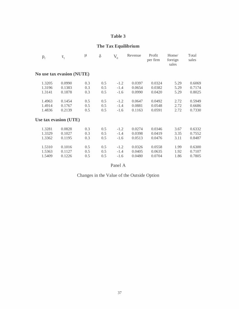
� Table�3�presents�several�sets�of�simulation�results.��Our�baseline�set�appear�in�
panel�A.��First,�we�confirm�our�intuition�that�use�tax�evasion�results�in�lower�equilibrium�
tax�revenue.��Note�that�this�occurs�for�two�reasons—some�sales�escape�taxation,�and�
equilibrium�tax�rates�are�lower.��Profits�are�higher�under�UTE.���
Tax�rates�rise�as�the�value�of�the�outside�option�falls�(as�the�total�demand�curve�
for�all�varieties�shift�out).��This�effect�is�considerably�more�pronounced�under�NUTE�than�
under�UTE.�With�total�sales�near�80%�of�consumers,�tax�rates�are�approximately�the�level�

� 16
of�EU�standard�VAT�rates.��Tax�rates�under�UTE�are�somewhat�higher�than�typical�state�
plus�local�sales�tax�rates�in�the�U.S.14�
One�difference�in�qualitative�comparative�statics�is�that�producer�prices�move�in�
opposite�directions�as�V0�changes�under�the�two�tax�regimes.��The�differential�magnitude�
of�the�tax�rate�changes�is�most�likely�a�cause.��Note�that�prices�change�only�slightly�with�
the�changes�in�V0;�as�with�zero�or�one�endogenous�tax�rate,�the�largest�impact�on�prices�
comes�from�changes�in�µ,�the�variety�parameter.��A�second�distinction�is�that�the�ratio�of�
home�to�foreign�sales�does�not�vary�with�tax�rates�and�V0�under�NUTE�due�to�the�
independence�of�irrelevant�alternatives�property�of�the�logit,�while�the�ration�of�home�to�
foreign�sales�moves�in�the�opposite�direction�of�the�tax�rate�under�UTE.�
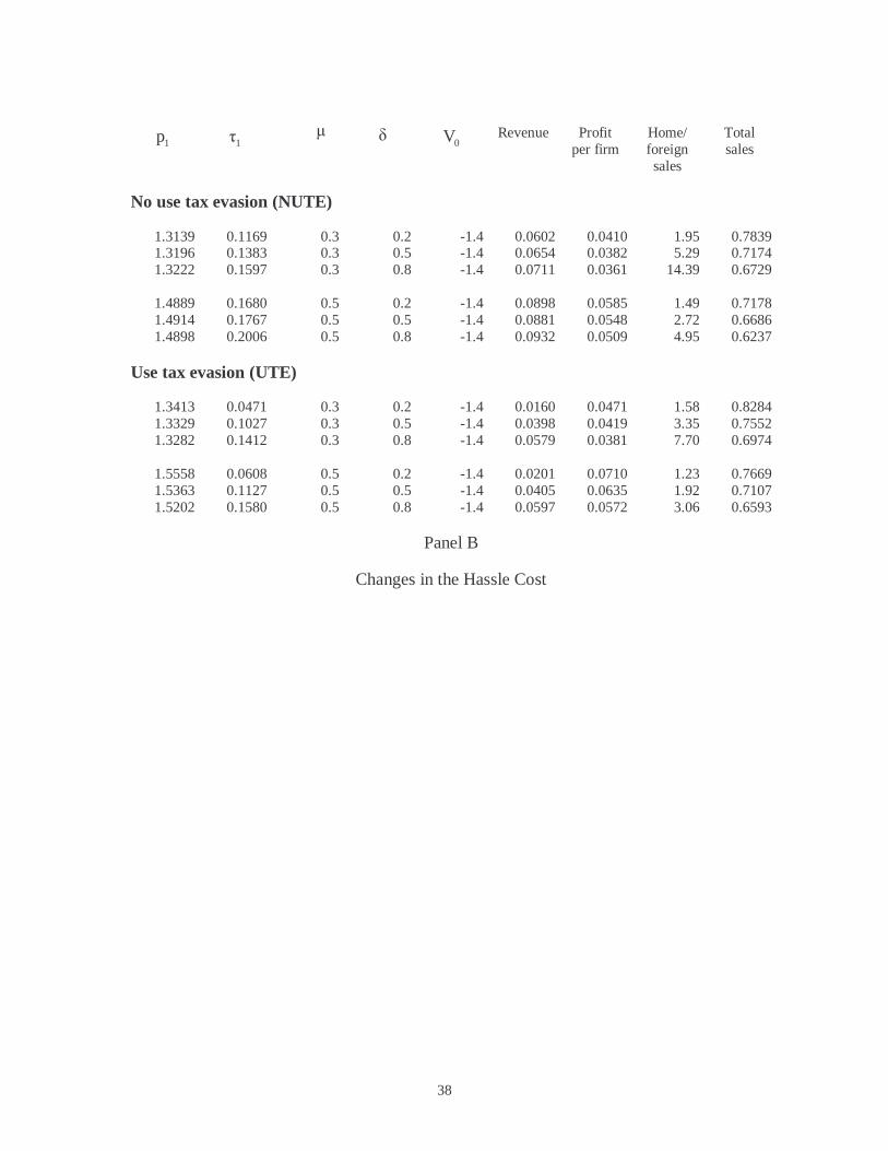
Panel�B�of�Table�3�displays�results�for�different�values�of�δ.��A�drop�in�δ�increases�
demand�directly�by�lowering�the�cost�of�some�varieties�at�constant�prices�and�taxes,�and�it�
also�makes�the�market�more�competitive�by�making�goods�from�firms�in�the�other�
jurisdiction�closer�substitutes�effectively.�
As�the�cost�of�cross-border�shopping�falls�from�80%�to�20%�of�the�good’s�
production�cost,��equilibrium�tax�rates�and�revenue�fall,�but�the�effect�is�greater�under�
UTE.��As�δ�falls�by�75%,�revenue�falls�by�only�15%�under�NUTE,�while�it�falls�by�72%�
under�UTE.�
As�δ�falls,�jurisdictions�face�more�pressure�to�lower�tax�rates�under�UTE.��Under�
NUTE,�this�direct�effect�is�not�present,�yet�tax�rates�still�fall�with�δ.��Producer�prices�fall�
slightly,�but�the�fall�in�consumer��prices�is�greater,�so�sales�and�profits�increase�
� �Panel�C�of�Table�3�displays�the�effect�of�changes�in�the�taste�for�variety�(µ).��As�
discussed�previously,�the�largest�impact�is�one�price-cost�margins.��Tax�rates�increase�as�

� 17
µ�rises,�as�we�should�expect.��As�demand�for�individual�firm’s�products�becomes�less�
elastic,�the�impact�of�taxes�on�sales�falls�in�magnitude,�which�frees�local�governments�to�
raise�tax�rates.��The�ratio�of�home�to�foreign�sales�falls�considerably�as�µ�rises�because�
consumers�resort�to�cross-border�shopping�to�obtain�a�greater�selection�of�varieties.�
�� �
7.��Further�Research�
� A�number�of�additional�questions�can�be�studied�in�this�framework.��First,�how�
does�the�relative�size�of�jurisdictions�and�the�number�of�retailers�in�each�affect�
equilibrium�tax�rates�and�revenues?��Second,�how�do�these�taxes�influence�firms’�location�
choices�when�jurisdictions�are�not�identical?��States�with�large�populations�may�be�
affected�much�differently�than�states��with�small�populations.��Another�issue�to�is�
compare�these�sales�taxes�to�production-based�taxes.�
The�answers�to�these�additional�questions�will�shed�some�light�on�future�tax�
policy,�including�the�role�of�sales�taxes�as�electronic�commerce�grows.��Since�one�
alternative�(at�least�within�the�U.S.)�is�to�substitute�a�Federal�sales�tax�for�state�and�local�
taxes�on�Internet�transactions,�it�will�be�instructive�to�see�how�far�independently�set�tax�
rates�fall�from�current�levels�as�the�effect�of�distance�declines�to�low�levels.��We�will�also�
be�able�to�study�the�effect�of�centrally-set�uniform�tax�rates�and�alternative�tax�regimes�on�
the�competitiveness�of�electronic�commerce.�
�
�
�

� 18
���������������������������������������������������������������������������������������������������������������������������������������������������������������������1���Activities�such�as�advertising�in�newspapers�published�in�a�jurisdiction�are�not�sufficient�to�establish�nexus.��The�presence�of�manufacturing�or�retail�sales�establishments�does�establish�nexus,�so�that�mail-order�firms�may�face�several�different�tax�issues�in�choosing�the�location�of�their�facilities.��2���The�tax�advantages�of�mail-order�firms�may�have�prevented�the�spread�of�modern�logistical�techniques�to�conventional�retailers.��3��California�does�not�have�local�retail�sales�taxes�per�se,�but�a�portion�of�the�state�sales�tax�is�distributed�to�the�jurisdiction�where�the�sale�occurred.�Lewis�and�Barbour�[1999]�demonstrate�that�land-use�decisions�by�local�governments�are�affected�by�this�tax,�in�that�local�governments�appear�to�value�the�presence�of�retail�businesses�over�other�types�of�employment�(and�over�residential�uses).��4���The�Harmonized�Sales�Tax�(HST)�levied�in�the�Canadian�provinces�of�Newfoundland,�New�Brunswick,�and�Nova�Scotia�which�use�the�same�base�as�the�federal�GST�(Goods�and�Services�Tax)�is�another�example�of�destination-based�sales�taxes.��The�system�in�other�Canadian�provinces�is�the�same�as�that�in�the�U.S.�for�inter-provincial�transactions,�but�both�the�federal�GST�and�the�provincial�tax�is�collected�on�shipments�from�outside�Canada�by�Canada�Customs�and�Revenue.��For�shipments�to�Saskatchewan,�only�GST�is�collected.��5��See�the�Appendix�for�the�demand�functions�without�use�tax�evasion.��6�In�particular,�the�sum�of�two�log-concave�demand�functions�is�not�necessarily�log-concave.���7�For�comparison,�in�a�symmetric�homogeneous�product�Cournot�model�with�an�ad�valorem�tax�,�the�producer�price�falls�at�a�rate�less�than�1/(number�of�firms�+�2).��Thus�firms�in�our�model�absorb�more�of�the�tax.��8�In�some�earlier�simulation,�we�also�had�local�output�in�the�objective�functions�as�a�proxy�for�employment.��It�is�clear�from�public�debates�that�employment�often�weighs�heavily�for�policymakers�in�regional�development�issues.��9��Under�NUTE,�jurisdiction�1’s�tax�revenue�is�R1�=�τ1[p1(γN1Hi)�+�p2(γN2Fj)].��10�Obviously,�the�fraction�of�consumers�who�buy�any�variety�will�vary�considerably�across�product�class.��We�focus�below�on�the�ranges�that�yield�plausible�tax�rates�and�discuss�the�sensitivity�to�this�factor.��11�As�a�benchmark,�traditional�book�retailers�charge�a�40%�margin�over�the�wholesale�price.��Since�some�additional�costs�are�certainly�part�of�long-run�variable�cost,�we�consider�lower�margins�to�be�more�indicative�of�conditions�in�the�industry.��

� 19
���������������������������������������������������������������������������������������������������������������������������������������������������������������������12��With�more�weight�on�consumer�surplus�and�less�on�profit�(a1�=�0.60,�a2�=�0.3,�and�a3�=�0.10),��the�best�replies�slope�down�for�some�parameter�values.��13�With�more�weight�on�consumer�surplus�and�less�on�profit�(a1�=�0.60,�a2�=�0.3,�and�a3�=�0.10),�NUTE�best�replies�are�below�the�UTE�best�replies�for�some�parameter�values.��14�As�of�June�1995,�state�plus�local�general�sales�tax�rates�were�between�8%�and�9%�in�some�cities�in�the�following�states:��AL,�CA,�IL,�LA,�NY,�OK,�TN,�TX,�and�WA.��(Source,�Advisory�Commission�on�Intergovernmental�Relations,�Significant�Features�of�Fiscal�Federalism�1995,�Table�28,�available�at�http://www.library.unt.edu/gpo/acir/acir.html).��

References�
Anderson,�S.,�A.�de�Palma,�and��J.-F.�Thisse�(1992),�Discrete�Choice�Theory�of�Product��
Differentiation,�MIT�Press.�
Braid,�R.�(1987),�“The�Spatial�Incidence�of�Local�Retail�Taxation,”�Quarterly�Journal�of��
Economics�102:��881-891.�
Braid,�R.�(1993),�“Spatial�Competition�between�Jurisdictions�Which�Tax�Perfectly��
Competitive�Retail�(or�Production)�Centers,”�Journal�of�Urban�Economics��
34:��75-95.�
Goolsbee,�A.�(2000),��“In�a�World�Without�Borders:��The�Impact�of�Taxes�on�Electronic��
Commerce,”�Quarterly�Journal�of�Economics�115:��561-576.�
Goolsbee,�A.�(2001),�“The�Implications��of�Electronic�Commerce�for�Fiscal�Policy�(and��
Vice�Versa),”�Journal�of�Economic�Perspectives�15�(no.�1):��13-23.�
Kanbur,�R.�and�M.�Keen�(1993),�“Jeux�Sans�Frontieres:��Tax�Competition�and�Tax��
Coordination�When�Countries�Differ�in�Size,”�American�Economic�Review�83:��
877-892.�
Trandel,�G.�(1992),�“Evading�the�Use�Tax�on�Cross-Border�Sales:�Pricing�and�Welfare��
Effects,”�Journal�of�Public�Economics�49:��313-331.��
Trandel,�G.�(1994),��“Interstate�Commodity�Tax�Differentials�and�the�Distribution�of��
Residents,”�Journal�of�Public�Economics�53:��435-457.�
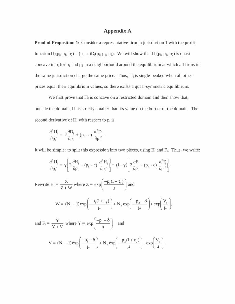
Appendix�A�
Proof�of�Proposition�1:��Consider�a�representative�firm�in�jurisdiction�1�with�the�profit�
function�Πi(pi,�p1,�p2)�=�(pi�-�c)Di(pi,�p1,�p2).��We�will�show�that�Πi(pi,�p1,�p2)�is�quasi-
concave�in�pi�for�p1�and�p2�in�a�neighborhood�around�the�equilibrium�at�which�all�firms�in�
the�same�jurisdiction�charge�the�same�price.��Thus,�Πi�is�single-peaked�when�all�other�
prices�equal�their�equilibrium�values,�so�there�exists�a�quasi-symmetric�equilibrium.�
� We�first�prove�that�Πi�is�concave�on�a�restricted�domain�and�then�show�that,�
outside�the�domain,�Πi�is�strictly�smaller�than�its�value�on�the�border�of�the�domain.��The�
second�derivative�of�Πi�with�respect�to�pi�is:�
�2
i2
ip
∂ Π∂
=� i
i
D2
p
∂∂
+�(pi�-�c)�2
i2
i
D
p
∂∂
.�
It�will�be�simpler�to�split�this�expression�into�two�pieces,�using�Hi�and�Fi.��Thus,�we�write:�
�2
i2
ip
∂ Π∂
=�2
i ii 2
i i
H H2 (p �-�c)�
p p
∂ ∂γ + ∂ ∂
+�2
i ii 2
i i
F F(1 ) 2 (p �-�c)�
p p
∂ ∂− γ + ∂ ∂
.�
Rewrite�Hi�=�Z
Z W+where�Z�≡� i 1p (1 )
exp− + τ
µ �and��
� � W�≡� 1 11
p (1 )(N 1)exp
− + τ − µ
µ
+
µ
δ−−+ 022
Vexp
pexpN ,��
and�Fi�=�Y
Y V+�where�Y�≡� ip
exp− − δ
µ � and��
� V�≡� 11
p(N 1)exp
− − δ − µ
µ
+
µ
τ+−+ 0222
Vexp
)1(pexpN .�

� 22
First,�2
i ii 2
i i
H H2 (p �-�c)�
p p
∂ ∂+
∂ ∂=�
( )( )
( )( )( )( )
1 i 1
22
1 WZ p c 1 W Z2
Z WZ W
+ τ − + τ −− + µ +µ +
.��The�term�in�
brackets�equals�( )( ) [ ]i 1
i
p c 12 1 2H
− + τ− + −
µ,�which�is�strictly�negative�for�pi�<�
1
2c
1
µ++ τ
.��Second,�2
i ii 2
i i
F F2 (p �-�c)�
p p
∂ ∂+
∂ ∂=�
( )( )( )
( )i
22
p c V YYV2
Y VY V
− −− + µ +µ +
.��The�
term�in�brackets�equals�( ) [ ]i
i
p c2 1 2F
−− + −
µ,�which�is�strictly�negative�for�pi�<�c�+�2µ.��
Since�the�sum�of�two�concave�functions�in�concave,�Πi�is�concave�on�the�smaller�of�these�
two�domains,�which�is�given�by�pi�<�1
2c
1
µ++ τ
.�
� For�pi�≥�1
2c
1
µ++ τ
,�we�can�examine�i
i
p∂Π∂
=�Di�+�(pi�-�c)�i
i
p
D
∂∂
=�
( ) ( ) ( )i ii i i i
i i
H FH p c 1 F p c
p p
∂ ∂γ + − + − γ + − ∂ ∂
.��Now,� ( ) ii i
i
HH p c
p
∂+ −
∂=�
( )( ) ( )i 1i
p c 1Z1 1 H
Z W
− + τ− − + µ
.��For�pi�≥�1
2c
1
µ++ τ
,�the�term�in�brackets�is�less�than�
or�equal�to�–1�+2Hi.��Similarly,� ( ) ii i
i
FF p c
p
∂+ −
∂=�
( ) ( )ii
p cY1 1 F
Y V
−− − + µ
.��For�pi��
≥1
2c
1
µ++ τ
,�the�term�in�brackets�is�less�than�or�equal�to� 1 i
1
1 2F
1
τ − ++ τ
.�
� The�symmetric�solution�to�the�FOC�yields�a�value�for�p1�and��p2�of�approximately�
1
c1
µ++ τ
�<�1
2c
1
µ++ τ
(which�is�the�upper�bound�for�the�region�where�Πi�is�concave�in�pi�

� 23
for�all�p1�and�p2).��Thus,�pi�>�p1�and�pi�>�p2�when�pi�≥�1
2c
1
µ++ τ
.��Now,�W�>�Z�and�V�>�Y�
for�N1�≥�2�whenever�pi�>�p1�(firm�i�charges�a�higher�price�than�its�rivals�in�the�same�
jurisdiction),�so�Hi�and�Fi�are�both�less�than�½�when�pi�>�p1.��Hence,�the�term�–1�+2Hi�is�
negative�for�pi�≥�1
2c
1
µ++ τ
.��Since�Fi�is�strictly�less�than�½,�the�term� 1 i
1
1 2F
1
τ − ++ τ
is�also�
negative�for�pi�≥�1
2c
1
µ++ τ
�as�long�as�the�tax�rate�is�less�than�a�threshold�value� τ̂ .��In�
practice,�this�threshold�can�be�quite�high:��for�δ�>�τ2p2,�Fi�<�1/(N1+N2)�when�pi�>�p1�=�p2,�
so�tax�rates�could�be�as�high�as�2/3�when�N1�=�N2�=�3�(as�we�use�in�our�simulations).��
Thus,�for�pi�≥�1
2c
1
µ++ τ
,�Πi(pi,�p1,�p2)�is�decreasing�in�pi.��
� Hence,�Πi�is�quasi-concave�in�pi,�so�there�exists�a�pure�strategy�Nash�equilibrium�
in�prices�for�min{N1,�N2}�≥�2�and�max{τ1,�τ2}�<� τ̂ .� � � � � QED�
�

� 24
Appendix�B�
Derivation�of�the�Subgame�Perfect�Nash�Equilibria�
The�timing�of�the�game�is�that�the�jurisdictions�choose�their�tax�rates,�and�then�the�
firms�choose�prices.��Let�τ1�be�the�tax�parameter�chosen�by�jurisdiction�1�and�τ2�be�the�tax�
parameter�chosen�by�jurisdiction�2.��Let�V1(p1,�p2;�τ1,�τ2)�and�V2(p1,�p2;�τ1,�τ2)�be�the�two�
jurisdictions’�objective�functions.���
� From�Section�4,�the�first-order�conditions�for�profit�maximization�are:�
i
i
p∂Π∂
=�Di�+�(pi�-�c)�i
i
p
D
∂∂
�=�0� and�j
j
p∂Π∂
=�Dj�+�(pj�-�c)�j
j
p
D
∂∂
=�0.� � � (A1)�
� The�FOC�for�the�lst�stage�game�are:� �
�1 1 1
1 2
1 1 1 2 1
p pV V V0
p p
∂ ∂∂ ∂ ∂+ + =∂τ ∂ ∂τ ∂ ∂τ
�
and�2 2 2
1 2
2 1 2 2 2
p pV V V0
p p
∂ ∂∂ ∂ ∂+ + =∂τ ∂ ∂τ ∂ ∂τ
�
We�find�the�terms� i
j
p∂∂τ
�by�totally�differentiating�the�price�equilibrium�subgame�FOC�
before�imposing�the�symmetry�conditions�pi�=�p1�and�pj�=�p2.��Totally�differentiate�(A1)�
w.r.t.�pi,�pj,�p1,�p2,�τk�(k�=�1�or�2)�to�obtain:�
� 11i
i2
i2i
i2
dppp
dpp ∂∂
Π∂+∂Π∂
�2 2 2
i i ij 2 k
i j i 2 i k
dp dp dp p p p p
∂ Π ∂ Π ∂ Π+ + = − τ∂ ∂ ∂ ∂ ∂ ∂τ
�
� 11j
j2
iij
j2
dppp
dppp ∂∂
Π∂+
∂∂Π∂ 2 2 2
j j jj 2 k2
j 2 j kj
dp dp dp p pp
∂ Π ∂ Π ∂ Π+ + = − τ
∂ ∂ ∂ ∂τ∂�
Now�we�can�impose�symmetry�within�a�jurisdiction�to�get�the�matrix�equation:�

� 25
�
∂∂Π∂
+∂Π∂
∂∂Π∂
+∂∂Π∂
∂∂Π∂
+∂∂Π∂
∂∂Π∂
+∂Π∂
2
1
2j
j2
2j
j2
1j
j2
ij
j2
2i
i2
ji
i2
1i
i2
2i
i2
dp
dp�
ppp����������
pppp�
pppp������������
ppp�
2i
i k
k2j
j k
p�d �������k 1,�2
p
∂ Π− ∂ ∂τ = τ = ∂ Π −
∂ ∂τ
�
and�use�Cramer’s�Rule�to�get�the�needed�comparative�statics�derivatives:�
� 1
1
p∂∂τ
,�� 2
1
p∂∂τ
�,� 1
2
p∂∂τ
�,�and�� 2
2
p∂∂τ
.�
Ordinarily,�ji
i2
pp ∂∂Π∂
�and�ij
j2
pp ∂∂Π∂
�are�both�identically�zero,�but�that�may�not�hold�across�all�
demand�structures.���
� The�second�derivatives�in�the�matrix�equation�(using�the�modular�forms)�are:1�
�2i
i2
ii
i2i
i2
p
D)cp(
p
D2
p ∂∂
−+∂∂
=∂Π∂
�
�1i
i2
i1
i
1i
i2
pp
D)cp(
p
D
pp ∂∂∂
−+∂∂
=∂∂Π∂
�
�2i
i2
i2
i
2i
i2
pp
D)cp(
p
D
pp ∂∂∂
−+∂∂
=∂∂Π∂
�
�1j
j2
j1
j
1j
j2
pp
D)cp(
p
D
pp ∂∂∂
−+∂∂
=∂∂Π∂
�
�2j
j2
jj
j
2j
j2
p
D)cp(
p
D2
p ∂∂
−+∂∂
=∂Π∂
�
��������������������������������������������������������
1�Note�i
i
1
i
p
D
p
D
∂∂≠
∂∂
�and�1i
i2
2i
i2
pp
D
p
D
∂∂∂
≠∂∂
despite�the�symmetry,�because�we�need�to�evaluate�the�
response�to�an�independent�deviation�by�firm�i.�
�

� 26
�2j
j2
j2
j
2j
j2
pp
D)cp(
p
D
pp ∂∂∂
−+∂∂
=∂∂Π∂
�
�2 2
i i ii
i k k i k
D D(p c)
p p
∂ Π ∂ ∂= + −
∂ ∂τ ∂τ ∂ ∂τ� k�=�1,�2�
and�2 2
j j jj
j k k j k
D D(p c)
p p
∂ Π ∂ ∂= + −
∂ ∂τ ∂τ ∂ ∂τ� k�=�1,�2.�
Derivatives�of�equilibrium�prices�
� Rewrite�the�matrix�equations�for�derivatives�of�the�equilibrium�prices�as:�
�
2
1
43
21
dpdp
AAAA
�=�
ττ
1
1
12
11
dd
BB
�+�
ττ
2
2
22
21
dd
BB
.�
�Using�Cramer’s�Rule,�we�obtain:��
�3241
212411
1
1
AAAA
ABAB
d
dp
−−=
τ�� �
3241
311112
1
2
AAAA
ABAB
d
dp
−−=
τ�
�
�3241
222421
2
1
AAAA
ABAB
d
dp
−−=
τ�� and�
3241
321122
2
2
AAAA
ABAB
d
dp
−−=
τ.�
��

� 27
Full�Use�Tax�Evasion��
� The�necessary�demand�derivatives�for�the�solution�of�the�two-stage�game�are:�
∂∂
γ−+
∂∂
γ=∂∂
i
i
i
i
i
i
p
F)1(
p
H
p
D�
∂∂
µτ++
∂∂
µτ+−γ=
∂∂
i
ii
1
i
i12i
i2
p
HH
)1(2
p
H)1(
p
D
∂∂
µ+
∂∂
µ−γ−+
i
ii
i
i
p
FF
2
p
F1)1( �
2i
1i
1
i
i )H()1(
H)1(
p
H
µτ++
µτ+−=
∂∂
�
2ii
i
i )F(1
F1
p
F
µ+
µ−=
∂∂
�
1
i
1
i
1
i
p
F)1(
p
H
p
D
∂∂γ−+
∂∂γ=
∂∂
�
µ
τ+−µτ+
−∆
=∂∂ )1(p
exp)1(
)1N(H
p
H 1111
1i
i
1
i �
µ
δ−−µ−
∆=
∂∂ 11
2i
i
1
i pexp
)1N(F
p
F�
∂∂
∂γ−+
∂∂
∂γ=
∂∂∂
1i
i2
1i
i2
1i
i2
pp
F)1(
pp
H
pp
D�
1
ii
1
1
i1
1i
i2
p
HH
)1(2
p
H)1(
pp
H
∂∂
µτ+
+∂∂
µτ+−
=∂∂
∂�
1
ii
1
i
1i
i2
p
FF
2
p
F1
pp
F
∂∂
µ+
∂∂
µ−=
∂∂∂
�
2
i
2
i
2
i
p
F)1(
p
H
p
D
∂∂γ−+
∂∂γ=
∂∂
�
µ
δ−−µ∆
=∂∂ 22
1i
i
2
i pexp
NH
p
H�

� 28
µ
τ+−µ
τ+∆
=∂∂ )1(p
exp)1(NF
p
F 2222
2i
i
2
i �
∂∂
µτ+
+∂∂
µτ+
−γ=∂∂
∂
2
ii
1
2
i1
2i
i2
p
HH
)1(2
p
H)1(
pp
D
∂∂
µ+
∂∂
µ−γ−+
2
ii
2
i
p
FF
2
p
F1)1( �
µ
τ+−∆µ
γ−=τ∂∂
γ−=τ∂
∂ )1(pexp
FpN)1(
F)1(
D 22
2i
i22
2
i
2
i �
1
i
1
i HD
τ∂∂γ=
τ∂∂
�
µτ+−
µ−
∆−
µ−=
τ∂∂ )1(
pexppH
HpH 1
ii
1i
ii
i
1
i
µ
τ+−µ−− )1(p
expp)1N( 1111 �
� =� ii H
p
µ− �+� 2
ii H
p
µ+�
µ
τ+−∆µ
− )1(pexp
H)1N(p 11
1i
i11 �
µ
+µ
−τ∂
∂µτ++
τ∂∂
µτ+−γ=
τ∂∂∂ 2
ii
1
ii
1
1
i1
1i
i2 HHH
H)1(2H)1(
p
D�
τ∂∂
µ+
τ∂∂
µ−γ−=
τ∂∂∂
2
ii
2
i
2i
i2 F
F2F1
)1(p
D�
The�demand�derivatives�for�the�representative�firm�in�jurisdiction�2�are�similar.�
�
No�Use�Tax�Evasion�
� We�can�write�the�demand�for�firm�i�in�jurisdiction�1�as�the�sum�of�two�
components,�“home”�and�“foreign”�demand,�or:� � �
� Di�=�γHi�+�(1�−�γ)Fi� � where� �1i
1i
i
)1(pexp
H∆
µ
τ+−
= �

� 29
� �
µ
τ+−−+
µ
τ+−=∆
)1(pexp)1N(
)1(pexp 11
11i
1i � � � �
� � � �
µ
+
µ
δ−τ+−+ 0122
Vexp
)1(pexpN �
� �2i
2i
i
)1(pexp
F∆
µ
δ−τ+−
= �
and� � ∆i2�=�exp
µ
δ−τ+−−+
µ
δ−τ+− )1(p)1N(
)1(p 211
2i �
� � � �
µ
+
µ
τ+−+ 0222
Vexp
)1(pexpN .�
�For�the�representative�firm�j�in�jurisdiction�2:�
� Dj�=�γFj�+�(1�-�γ)Hj� � where�2j
2j
j
)1(pexp
H∆
µ
τ+−
= �
� �
µ
τ+−−+
µ
δ−τ+−=∆ )1(pexp)1N(
)1(pexpN 22
221
12j � � �
� � � �
µ
+
µ
τ+−+ o2j V
exp)1(p
exp �
1j
1j
j
)1(pexp
F∆
µ
δ−τ+−
= �
� � ∆j1�=�N1�exp�
µ
δ−τ+−−+
µ
τ+− )1(pexp)1N(
)1(p 122
11 �
� � � � +�exp
µ
+
µ
δ−τ+−o1j V
exp)1(p
.�

� 30
We�do�not�present�the�demand�derivatives�for�firm�j�here,�but�the�authors�will�supply�
them�upon�request.�
The�Jurisdictions’�Objective�Functions�under�Use�Tax�Evasion��Revenue��� The�revenue�maximization�problem�for�jurisdiction�1�is:�
���1
Maxτ
�R1�=��τ1N1piγHi(pi,�p1,�p2�;�τ1)�
with�the�first�derivative:�
1
1
1
R
N
1
τ∂∂
γ=�piHi(pi,�p1,�p2�;�τ1)�+�τ1pi
1
iH
τ∂∂
+�[τ1Hi�(pi,�p1,�p2�;�τ1)�+�τ1pii
i
p
H
∂∂
�+��
τ1pi1
i
p
H
∂∂
]1
1p
τ∂∂
��+�[τ1p12
i
p
H
∂∂
]1
2p
τ∂∂
.�
Note�that�i
i
p
H
∂∂
�is�the�effect�on�demand�for�firm�i’s�product�of�a�change�in�its�own�price,�
while�1
i
p
H
∂∂
is�the�effect�on�its�demand�of�a�change�in�the�price�charged�by�all�its�rivals�in�
jurisdiction�1.��Since�pi�=�p1�in�the�subgame-perfect�equilibrium,�1
ip
τ∂∂
�=�1
1p
τ∂∂
.�
Consumer�Surplus�� �
� Consumers�in�jurisdiction�1�choose�among�N1�firms�in�jurisdiction�1�and�N2�firms�
in�jurisdiction�2.��Thus,�
� S1�=�
µ
+
µ
+
µ
µ 0122
111
Vexp
uexpN
uexpNln �
� � � where�u11�=�-p1(1+τ1)���and�u12�=�-p2-δ�

� 31
Similarly,�S2�=�
µ
+
µ
+
µ
µ 0211
222
Vexp
uexpN
uexpNln �
� � � where�u22�=�-p2(1+τ2)���and�u21�=�-p1-δ.�
Prices�are�the�equilibrium�prices:� ),(p 21*1 ττ �and� ),(p 21
*2 ττ .�
The�derivatives�of�surplus�with�respect�to�own�tax�rates�are:�
1
1S
τ∂∂
=
µ
+
µ
+
µ
τ∂
∂−
µµ
+τ∂∂τ+−−
µµ
µ
0122
111
1
2122
1
111
111
Vexp
uexpN
uexpN
)p
(u
expN
)p
)1(p(u
expN
�
� =�
µ
+
µ
+
µ
τ∂
∂−
µ
+τ∂∂τ+−−
µ
0122
111
1
2122
1
111
111
Vexp
uexpN
uexpN
)p
(u
expN)p
)1(p(u
expN
�
and��
2
2S
τ∂∂
=
µ
+
µ
+
µ
τ∂∂−
µµ
+τ∂∂τ+−−
µµ
µ
0211
222
2
1211
2
222
222
Vexp
uexpN
uexpN
)p
(u
expN
)p
)1(p(u
expN
�
� =�
µ
+
µ
+
µ
τ∂∂−
µ
+τ∂∂τ+−−
µ
0211
222
2
1211
2
222
222
Vexp
uexpN
uexpN
)p
(u
expN)p
)1(p(u
expN
.�
Profits��� Total�profits�of�firms�producing�in�jurisdiction�1�equals:�
� Π1�=��(pi�-�c)N1{γHi(pi,�p1,�p2;�τ1,�τ2)��+�(1�−�γ)Fi(pi,�p1,�p2;�τ1,�τ2)}�
and�total�profits�of�firms�producing�in�jurisdiction�2�equals:�
� Π2�=�(pj�-�c)N2{γFj(pj,�p1,�p2;�τ1,�τ2)��+�(1�−�γ)Hj(pj,�p1,�p2;�τ1,�τ2)}.�

� 32
The�derivatives�of�profits�with�respect�to�own�tax�rates�are�then:�
�1
1
1N
1
τ∂Π∂
=� ( )ii1
1 F)1(Hp γ−+γτ∂∂
�+� ( )
τ∂∂+
τ∂∂
∂∂+
τ∂∂
∂∂+
∂∂−γ
1
i
1
2
2
i
1
1
1
i
i
i1i
Hp
p
Hp
p
H
p
Hcp �
� � +�( )( )
τ∂∂
∂∂+
τ∂∂
∂∂+
∂∂−γ−
1
2
2
i
1
1
1
i
i
i1i
p
p
Fp
p
F
p
Fcp1 �
�2
2
2N
1
τ∂Π∂
=� ( )jj2
2 H)1(Fp γ−+γτ∂∂
�+� ( )
τ∂∂
∂∂
+τ∂∂
∂∂
+∂∂
−γ2
1
1
j
2
2
2
j
j
j2j
p
p
Fp
p
F
p
Fcp �
� � + ( )
τ∂∂
+τ∂∂
∂∂
+τ∂∂
∂∂
+∂∂
−γ−2
j
2
1
1
j
2
2
2
j
j
j2j
Hp
p
Hp
p
H
p
Hcp1 )( �

� 33
�Table�1�
� � � � � � �Equilibrium�Prices�for�Different�Tax�Rates�
� � � � � � �No�use�tax�evasion�(NUTE)� � � �
� � � � � � �
1p � 2p � ������ 1τ � ������ 2τ � ��������µ � ��������δ �0V �
� � � � � � �1.3485� 1.3536� 0.05� 0.00� 0.3� 0.2� -1.6�1.3420� 1.3420� 0.05� 0.05� 0.3� 0.2� -1.6�1.3312� 1.3360� 0.10� 0.05� 0.3� 0.2� -1.6�1.3253� 1.3253� 0.10� 0.10� 0.3� 0.2� -1.6�1.3153� 1.3198� 0.15� 0.10� 0.3� 0.2� -1.6�1.3100� 1.3100� 0.15� 0.15� 0.3� 0.2� -1.6�1.3050� 1.3006� 0.15� 0.20� 0.3� 0.2� -1.6�
� � � � � � �1.3806� 1.3999� 0.05� 0.00� 0.3� 0.8� -1.6�1.3792� 1.3792� 0.05� 0.05� 0.3� 0.8� -1.6�1.3601� 1.3780� 0.10� 0.05� 0.3� 0.8� -1.6�1.3589� 1.3589� 0.10� 0.10� 0.3� 0.8� -1.6�1.3412� 1.3579� 0.15� 0.10� 0.3� 0.8� -1.6�1.3402� 1.3402� 0.15� 0.15� 0.3� 0.8� -1.6�1.3393� 1.3237� 0.15� 0.20� 0.3� 0.8� -1.6�
� � � � � � �1.5674� 1.5725� 0.05� 0.00� 0.5� 0.2� -1.6�1.5555� 1.5555� 0.05� 0.05� 0.5� 0.2� -1.6�1.5395� 1.5443� 0.10� 0.05� 0.5� 0.2� -1.6�1.5287� 1.5287� 0.10� 0.10� 0.5� 0.2� -1.6�1.5140� 1.5185� 0.15� 0.10� 0.5� 0.2� -1.6�1.5041� 1.5041� 0.15� 0.15� 0.5� 0.2� -1.6�1.4949� 1.4907� 0.15� 0.20� 0.5� 0.2� -1.6�
� � � � � � �1.5882� 1.6094� 0.05� 0.00� 0.5� 0.8� -1.6�1.5827� 1.5827� 0.05� 0.05� 0.5� 0.8� -1.6�1.5583� 1.5779� 0.10� 0.05� 0.5� 0.8� -1.6�1.5534� 1.5534� 0.10� 0.10� 0.5� 0.8� -1.6�1.5309� 1.5491� 0.15� 0.10� 0.5� 0.8� -1.6�1.5265� 1.5265� 0.15� 0.15� 0.5� 0.8� -1.6�1.5226� 1.5057� 0.15� 0.20� 0.5� 0.8� -1.6�
� � � � � � �� � � � � � �� � � � � � �� � � � � � �� � � � � � ����������
� � � � � �

� 34
� � � � � � �Use�Tax�evasion�(UTE)� � � �
� � � � � � �
1p � 2p � ������ 1τ � ������ 2τ � ��������µ � ��������δ �0V �
� � � � � � �1.3453� 1.3601� 0.05� 0.00� 0.3� 0.2� -1.6�1.3458� 1.3458� 0.05� 0.05� 0.3� 0.2� -1.6�1.3334� 1.3468� 0.10� 0.05� 0.3� 0.2� -1.6�1.3350� 1.3350� 0.10� 0.10� 0.3� 0.2� -1.6�1.3248� 1.3369� 0.15� 0.10� 0.3� 0.2� -1.6�1.3273� 1.3273� 0.15� 0.15� 0.3� 0.2� -1.6�1.3300� 1.3193� 0.15� 0.20� 0.3� 0.2� -1.6�
� � � � � � �1.3790� 1.3998� 0.05� 0.00� 0.3� 0.8� -1.6�1.3778� 1.3778� 0.05� 0.05� 0.3� 0.8� -1.6�1.3577� 1.3765� 0.10� 0.05� 0.3� 0.8� -1.6�1.3566� 1.3566� 0.10� 0.10� 0.3� 0.8� -1.6�1.3384� 1.3557� 0.15� 0.10� 0.3� 0.8� -1.6�1.3377� 1.3377� 0.15� 0.15� 0.3� 0.8� -1.6�1.3370� 1.3212� 0.15� 0.20� 0.3� 0.8� -1.6�
� � � � � � �1.5651� 1.5852� 0.05� 0.00� 0.5� 0.2� -1.6�1.5661� 1.5661� 0.05� 0.05� 0.5� 0.2� -1.6�1.5493� 1.5673� 0.10� 0.05� 0.5� 0.2� -1.6�1.5511� 1.5511� 0.10� 0.10� 0.5� 0.2� -1.6�1.5368� 1.5530� 0.15� 0.10� 0.5� 0.2� -1.6�1.5393� 1.5393� 0.15� 0.15� 0.5� 0.2� -1.6�1.5419� 1.5274� 0.15� 0.20� 0.5� 0.2� -1.6�
� � � � � � �1.5856� 1.6130� 0.05� 0.00� 0.5� 0.8� -1.6�1.5842� 1.5842� 0.05� 0.05� 0.5� 0.8� -1.6�1.5583� 1.5830� 0.10� 0.05� 0.5� 0.8� -1.6�1.5574� 1.5574� 0.10� 0.10� 0.5� 0.8� -1.6�1.5344� 1.5567� 0.15� 0.10� 0.5� 0.8� -1.6�1.5341� 1.5341� 0.15� 0.15� 0.5� 0.8� -1.6�1.5339� 1.5135� 0.15� 0.20� 0.5� 0.8� -1.6�
�

� 35
�Table�2�
� � � � � � � � �Best�Replies�in�the�Tax�Game�
� � � � � � � � �No�use�tax�evasion�(NUTE)� � � � �
� � � � � � � � �
1p � 2p � ��� 1τ �
endo�–�genous�
���� 2τ �
������fixed�
���������µ � ���������δ � ��������� 0V � 1τ∆ *� ��Total�����sales�
� � � � � � � � �1.3217� 1.3251� 0.0775� 0.05� 0.3� 0.2� -1.2� � 0.6942�1.3153� 1.3130� 0.0813� 0.10� 0.3� 0.2� -1.2� � 0.6759�1.3095� 1.3020� 0.0854� 0.15� 0.3� 0.2� -1.2� 0.0079� 0.6560�
� � � � � � � � �1.3188� 1.3291� 0.1613� 0.05� 0.3� 0.2� -1.6� � 0.8750�1.3128� 1.3184� 0.1633� 0.10� 0.3� 0.2� -1.6� � 0.8673�1.3070� 1.3084� 0.1654� 0.15� 0.3� 0.2� -1.6� 0.0042� 0.8581�
� � � � � � � � �1.3233� 1.3469� 0.1149� 0.05� 0.3� 0.8� -1.2� � 0.5863�1.3218� 1.3276� 0.1165� 0.10� 0.3� 0.8� -1.2� � 0.5676�1.3206� 1.3100� 0.1179� 0.15� 0.3� 0.8� -1.2� 0.0030� 0.5484�
� � � � � � � � �1.3240� 1.3762� 0.2068� 0.05� 0.3� 0.8� -1.6� � 0.8032�1.3222� 1.3569� 0.2084� 0.10� 0.3� 0.8� -1.6� � 0.7923�1.3206� 1.3391� 0.2099� 0.15� 0.3� 0.8� -1.6� 0.0031� 0.7802�
� � � � � � � � �1.5158� 1.5241� 0.1280� 0.05� 0.5� 0.2� -1.2� � 0.6680�1.5038� 1.5072� 0.1328� 0.10� 0.5� 0.2� -1.2� � 0.6570�1.4927� 1.4915� 0.1376� 0.15� 0.5� 0.2� -1.2� 0.0096� 0.6452�
� � � � � � � � �1.5118� 1.5250� 0.1960� 0.05� 0.5� 0.2� -1.6� � 0.8002�1.5005� 1.5092� 0.1992� 0.10� 0.5� 0.2� -1.6� � 0.7934�1.4900� 1.4944� 0.2025� 0.15� 0.5� 0.2� -1.6� 0.0065� 0.7858�
� � � � � � � � �1.5126� 1.5353� 0.1359� 0.05� 0.5� 0.5� -1.2� � 0.6177�1.5037� 1.5140� 0.1409� 0.10� 0.5� 0.5� -1.2� � 0.6060�1.4955� 1.4945� 0.1458� 0.15� 0.5� 0.5� -1.2� 0.0099� 0.5938�
� � � � � � � � �1.5102� 1.5455� 0.2005� 0.05� 0.5� 0.5� -1.6� � 0.7620�1.5014� 1.5249� 0.2045� 0.10� 0.5� 0.5� -1.6� � 0.7540�1.4932� 1.5059� 0.2086� 0.15� 0.5� 0.5� -1.6� 0.0082� 0.7453�
� � � � � � � � �� � � � � � � � �
* 1τ∆ =�� τ1(.15)�-�� τ1(.05)� � � � � � �
� � � � � � � � �� � � � � � � � �
�����
� � � � � � � �
� � � � � � � � �� � � � � � � � �

� 36
Use�tax�evasion�(UTE)� � � � �� � � � � � � � �
1p � 2p � � 1τ � ������ 2τ � ���������µ � ���������δ � ��������� 0V � 1τ∆ � ���Tsales�
� � � � � � � � �1.3360� 1.3329� 0.0386� 0.05� 0.3� 0.2� -1.2� � 0.7189�1.3378� 1.3209� 0.0334� 0.10� 0.3� 0.2� -1.2� � 0.7103�1.3396� 1.3108� 0.0285� 0.15� 0.3� 0.2� -1.2� -0.0101� 0.7015�
� � � � � � � � �1.3451� 1.3459� 0.0526� 0.05� 0.3� 0.2� -1.6� � 0.9016�1.3481� 1.3333� 0.0446� 0.10� 0.3� 0.2� -1.6� � 0.8980�1.3513� 1.3221� 0.0369� 0.15� 0.3� 0.2� -1.6� -0.0157� 0.8941�
� � � � � � � � �1.3243� 1.3471� 0.1112� 0.05� 0.3� 0.8� -1.2� � 0.5945�1.3246� 1.3280� 0.1096� 0.10� 0.3� 0.8� -1.2� � 0.5791�1.3248� 1.3108� 0.1081� 0.15� 0.3� 0.8� -1.2� -0.0031� 0.5634�
� � � � � � � � �1.3281� 1.3745� 0.1823� 0.05� 0.3� 0.8� -1.6� � 0.8188�1.3287� 1.3552� 0.1785� 0.10� 0.3� 0.8� -1.6� � 0.8108�1.3294� 1.3374� 0.1745� 0.15� 0.3� 0.8� -1.6� -0.0078� 0.8021�
� � � � � � � � �1.5490� 1.5514� 0.0566� 0.05� 0.5� 0.2� -1.2� � 0.6933�1.5519� 1.5351� 0.0506� 0.10� 0.5� 0.2� -1.2� � 0.6883�1.5548� 1.5209� 0.0449� 0.15� 0.5� 0.2� -1.2� -0.0116� 0.6831�
� � � � � � � � �1.5600� 1.5665� 0.0674� 0.05� 0.5� 0.2� -1.6� � 0.8291�1.5641� 1.5496� 0.0593� 0.10� 0.5� 0.2� -1.6� � 0.8259�1.5683� 1.5345� 0.0515� 0.15� 0.5� 0.2� -1.6� -0.0160� 0.8225�
� � � � � � � � �1.5137� 1.5581� 0.1467� 0.05� 0.5� 0.8� -1.2� � 0.5908�1.5151� 1.5339� 0.1432� 0.10� 0.5� 0.8� -1.2� � 0.5831�1.5165� 1.5122� 0.1397� 0.15� 0.5� 0.8� -1.2� -0.0070� 0.5753�
� � � � � � � � �1.5180� 1.5811� 0.1891� 0.05� 0.5� 0.8� -1.6� � 0.7476�1.5203� 1.5563� 0.1832� 0.10� 0.5� 0.8� -1.6� � 0.7423�1.5225� 1.5339� 0.1775� 0.15� 0.5� 0.8� -1.6� -0.0116� 0.7367�
* 1τ∆ =�� τ1(.15)�-�� τ1(.05)� �
�
� 37
�Table�3�
� � � � � � � � �The�Tax�Equilibrium�
� � � � � � � � �
1p � 1τ � ��������µ � ��δ ������0V � Revenue� Profit�
per�firm�Home/�foreign�sales�
Total�sales�
� � � � � � � � �No�use�tax�evasion�(NUTE)� � � � �
� � � � � � � � �1.3205� 0.0990� 0.3� 0.5� -1.2� 0.0397� 0.0324� 5.29� 0.6069�1.3196� 0.1383� 0.3� 0.5� -1.4� 0.0654� 0.0382� 5.29� 0.7174�1.3141� 0.1878� 0.3� 0.5� -1.6� 0.0990� 0.0420� 5.29� 0.8025�
� � � � � � � � �1.4963� 0.1454� 0.5� 0.5� -1.2� 0.0647� 0.0492� 2.72� 0.5949�1.4914� 0.1767� 0.5� 0.5� -1.4� 0.0881� 0.0548� 2.72� 0.6686�1.4836� 0.2139� 0.5� 0.5� -1.6� 0.1163� 0.0591� 2.72� 0.7330�
� � � � � � � � �Use�tax�evasion�(UTE)� � � � �� � � � � � � � �
1.3281� 0.0828� 0.3� 0.5� -1.2� 0.0274� 0.0346� 3.67� 0.6332�1.3329� 0.1027� 0.3� 0.5� -1.4� 0.0398� 0.0419� 3.35� 0.7552�1.3362� 0.1195� 0.3� 0.5� -1.6� 0.0513� 0.0476� 3.11� 0.8487�
� � � � � � � � �1.5310� 0.1016� 0.5� 0.5� -1.2� 0.0326� 0.0558� 1.99� 0.6300�1.5363� 0.1127� 0.5� 0.5� -1.4� 0.0405� 0.0635� 1.92� 0.7107�1.5409� 0.1226� 0.5� 0.5� -1.6� 0.0480� 0.0704� 1.86� 0.7805�
� � � � � � � � �Panel�A�
� � � � � � � � �Changes�in�the�Value�of�the�Outside�Option�
������
� 38
�
1p � 1τ � ��������µ � ��δ ������0V � Revenue� Profit�
per�firm�Home/�foreign�sales�
Total�sales�
� � � � � � � � �No�use�tax�evasion�(NUTE)� � � � �� � � � � � � � �
1.3139� 0.1169� 0.3� 0.2� -1.4� 0.0602� 0.0410� 1.95� 0.7839�1.3196� 0.1383� 0.3� 0.5� -1.4� 0.0654� 0.0382� 5.29� 0.7174�1.3222� 0.1597� 0.3� 0.8� -1.4� 0.0711� 0.0361� 14.39� 0.6729�
� � � � � � � � �1.4889� 0.1680� 0.5� 0.2� -1.4� 0.0898� 0.0585� 1.49� 0.7178�1.4914� 0.1767� 0.5� 0.5� -1.4� 0.0881� 0.0548� 2.72� 0.6686�1.4898� 0.2006� 0.5� 0.8� -1.4� 0.0932� 0.0509� 4.95� 0.6237�
� � � � � � � � �Use�tax�evasion�(UTE)� � � � �� � � � � � � � �
1.3413� 0.0471� 0.3� 0.2� -1.4� 0.0160� 0.0471� 1.58� 0.8284�1.3329� 0.1027� 0.3� 0.5� -1.4� 0.0398� 0.0419� 3.35� 0.7552�1.3282� 0.1412� 0.3� 0.8� -1.4� 0.0579� 0.0381� 7.70� 0.6974�
� � � � � � � � �1.5558� 0.0608� 0.5� 0.2� -1.4� 0.0201� 0.0710� 1.23� 0.7669�1.5363� 0.1127� 0.5� 0.5� -1.4� 0.0405� 0.0635� 1.92� 0.7107�1.5202� 0.1580� 0.5� 0.8� -1.4� 0.0597� 0.0572� 3.06� 0.6593�
� � � � � � � � �Panel�B�
� � � � � � � � �Changes�in�the�Hassle�Cost�
�

� 39
�
1p � 1τ � ��������µ � ��δ ������0V � Revenue� Profit�
per�firm�Home/�foreign�sales�
Total�sales�
� � � � � � � � �No�use�tax�evasion�(NUTE)� � � � �� � � � � � � � �
1.3139� 0.1169� 0.3� 0.2� -1.4� 0.0602� 0.0410� 1.95� 0.7839�1.4036� 0.1411� 0.4� 0.2� -1.4� 0.0737� 0.0501� 1.65� 0.7443�1.4889� 0.1680� 0.5� 0.2� -1.4� 0.0898� 0.0585� 1.49� 0.7178�
� � � � � � � � �1.3196� 0.1383� 0.3� 0.5� -1.4� 0.0654� 0.0382� 5.29� 0.7174�1.4071� 0.1556� 0.4� 0.5� -1.4� 0.0752� 0.0466� 3.49� 0.6868�1.4914� 0.1767� 0.5� 0.5� -1.4� 0.0881� 0.0548� 2.72� 0.6686�
� � � � � � � � �Use�tax�evasion�(UTE)� � � � �� � � � � � � � �
1.3413� 0.0471� 0.3� 0.2� -1.4� 0.0160� 0.0471� 1.58� 0.8284�1.4489� 0.0532� 0.4� 0.2� -1.4� 0.0176� 0.0592� 1.36� 0.7916�1.5558� 0.0608� 0.5� 0.2� -1.4� 0.0201� 0.0710� 1.23� 0.7669�
� � � � � � � � �1.3329� 0.1027� 0.3� 0.5� -1.4� 0.0398� 0.0419� 3.35� 0.7552�1.4343� 0.1070� 0.4� 0.5� -1.4� 0.0393� 0.0526� 2.38� 0.7272�1.5363� 0.1127� 0.5� 0.5� -1.4� 0.0405� 0.0635� 1.92� 0.7107�
� � � � � � � � �Panel�C�
� � � � � � � � �Changes�in�the�Value�of�Diversity�
����
�
�