Dynamic Spatial Competition Between Multi‐Store...

DYNAMIC SPATIAL COMPETITION BETWEENMULTI-STORE RETAILERS*

VICTOR AGUIRREGABIRIA†

GUSTAVO VICENTINI‡

We propose a dynamic model of an oligopoly industry characterized byspatial competition between multi-store retailers. Firms compete inprices and decide where to open or close stores depending on demandand cost conditions, the number of competitors at different locations,and on location-specific private-information shocks. The modeldistinguishes multiple forces in the spatial configuration of storenetworks, such as cannibalization of revenue between stores of the sameretail chain, economies of density, competition, consumer transportationcosts, or positive demand spillovers from other stores. We develop analgorithm to approximate a Markov Perfect Equilibrium in our model,and propose a procedure for the estimation of the parameters of themodel using panel data on number of stores, prices, and quantities atmultiple geographic locations within a city. We also present a numericalexample to illustrate the model and algorithm.

I. INTRODUCTION

RETAIL CHAINS ACCOUNT FOR MORE THAN 60% OF SALES IN U.S. RETAILING

(see Hollander and Omura [1989], and Jarmin, Klimek and Miranda[2009]). Geographic location is in many cases the most important source ofproduct differentiation for these firms. It is also a forward looking decisionwith significant non-recoverable entry costs, mainly due to capital invest-ments which are both firm and location specific. Thus, the sunk cost of set-ting up a new store, and the dynamic strategic behavior associated withthem, is a potentially important force behind the configuration of the spa-tial market structure that we observe in retail markets.

Despite its relevance, there have been very few studies analyzing spatialcompetition as a dynamic oligopoly game. Existent models of industry

*This paper has benefited of comments from the Editor and two anonymous referees,and from conversations with Allan Collard-Wexler, Deniz Corbaci, Federico Echenique,Tom Holmes, Aviv Nevo, Stephen Ryan, Junichi Suzuki, and Xavier Vives, and from semi-nar participants at the Federal Trade Commission, NYU-Stern, Purdue University, and atthe Supermarkets conference organized by ELSE-IFS in London.

†Authors� affiliations: Department of Economics, University of Toronto, and CEPR.,150 St. George Street, Toronto, Ontario, Canada.e-mail: [email protected]

‡Department of Economics, Northeastern University, 301 Lake Hall, Boston,Massachusetts, U.S.A.e-mail: [email protected]

VC 2016 The Editorial Board of The Journal of Industrial Economics and John Wiley & Sons Ltd

710

THE JOURNAL OF INDUSTRIAL ECONOMICS 0022-1821Volume LXIV December 2016 No. 4

dynamics often lack an explicit account of spatial competition. Althoughuseful applications have emerged from the seminal work by Pakes andMcGuire [1994] and Ericson and Pakes [1995], none have explicitly incor-porated the spatial and multi-store features which are prevalent in manyretailing industries.1 The literature on spatial competition often restrictsthe treatment of time. Models based on the seminal work of Hotelling[1929] describe a two or three-period framework where firms choose loca-tions and then compete in the product market.2 Eaton and Lipsey [1975],Schmalensee [1978], and Bonanno [1987] study the multi-store monopolistunder the threat of entry. They find that an incumbent monopolist willstrategically locate its stores to successfully preempt the entry of competi-tors. As noted by Judd [1985], the limited account of time and dynamics inthis literature has very important implications on some predictions of thesemodels. Judd notes that the aforementioned models assume that entry andlocation decisions are completely irreversible, with no possibility of exit orrelocation. He shows that allowing for exit may result in non-successfulspatial preemption by the incumbent. Judd�s paper emphasizes that modelsof spatial competition between multi-store firms need to incorporatedynamics to its full extent, allowing for endogenous entry, exit, andforward-looking strategies. That is the intention of this paper.

In this context, the contribution of this paper is threefold. First, we pro-pose a dynamic model of an oligopoly industry characterized by spatialcompetition between multi-store firms. In this model, firms compete in pri-ces and decide where to open or close stores depending on the location pro-file of competitors, demand and cost conditions, and location-specificprivate information shocks. The model distinguishes multiple forces in thespatial configuration of store networks, such as cannibalization of revenuebetween stores of the same retail chain, economies of density, competition,consumer transportation costs, or positive demand spillovers from otherstores. We define and characterize a Markov Perfect Equilibrium (MPE) inthis model. The consideration of multi-store retail firms is a particularly rele-vant aspect of our model. Important topics in the analysis of competition inretail industries, such as cannibalization, spatial pre-emption, economies ofdensity, network effects, or the value of mergers between store networks,

1 Ellickson, Beresteanu and Misra [2010] endogenize supermarkets� �store density,� i.e., thenumber of stores per capita a firm owns in a market. Holmes [2011] studies the role of econo-mies of density in explaining the spatial evolution of Wal-Mart stores since the 1950s. How-ever, spatial competition is not accounted for in these applications.

2 Anderson, De Palma and Thisse [1992] present a compilation of static spatial competitionmodels. There is also a large and growing literature on estimation of static structural modelsof spatial competition and store location. The work by West [1981a] and [1981b] was seminalin this literature. Some recent important contributions to this empirical literature are Pinkse,Slade and Brett [2002], Seim [2006], Zhu and Singh [2009], Ellickson, Houghton and Timmins[2013], Datta and Sudhir [2011], and Vitorino [2012]. Slade [2005] and Pinkse and Slade[2010] provide excellent surveys.

DYNAMIC SPATIAL COMPETITION BETWEEN BIG RETAILERS 711


cannot be studied without a model that recognizes the multi-store nature ofretailers. Until recently, empirical games of market entry and store locationdid not account for the explicit multi-store nature of retailers, e.g., Seim[2006] and Zhu and Singh [2009]. However, recent studies by Jia [2008],Ellickson, Houghton and Timmins [2013], and Nishida [2014] propose andestimate entry games between retail chains. Our paper extends the models inthese three previous papers in several important dimensions. First, whilethese previous models are static, we consider a dynamic game. Incorporatingdynamics and firms� forward looking behavior is necessary to study topicssuch as pre-emption, first-mover advantage, or the implications of firms�uncertainty about future demand or land price. Second, the models in theseprevious papers do not incorporate spatial differentiation and competitionwithin a market (i.e., within a U.S. county in the papers by Jia [2008] andEllickson, Houghton and Timmins [2013], and within a 1 km square regionin the paper by Nishida [2014]). In contrast, our model incorporates spatialdifferentiation and the explicit distance between retailers� stores within a citysuch that we can measure the degree of spatial substitution between stores.Third, Jia [2008] and Ellickson, Houghton and Timmins [2013] impose therestriction that there are only positive (or only negative) spillover effectsbetween stores of the same retail chain. Our model allows for both cannibal-ization effects on the demand side and economies of scope, scale and densityon the cost side.3 Finally, the specification of the profit function in these pre-vious models is semi-structural in the sense that it does not distinguishbetween demand and cost parameters. Our framework includes an explicitmodel of consumer demand with spatial differentiation, and a model of pricecompetition between multi-store retailers. This allows us to distinguishbetween demand, variable cost, fixed cost and entry cost parameters, and tostudy welfare implications of alternative policies or firms� strategies.

A second contribution of this paper is to provide a method to compute anequilibrium of the model. The number of possible geographic configurationsof a store network, that determines the size of the action space and of the statespace in this dynamic game, increases exponentially with the number of geo-graphic locations and with the number of firms. Solving exactly for an equilib-rium of the model is an intractable problem even when the number oflocations is not too large.4 In static games of network competition, recentpapers have proposed models and methods to deal with the high dimensional-ity of the action space. Jia [2008] and Nishida [2014] show that under certainrestrictions on the profit function the static game is supermodular and this

3 The model in Nishida [2014] allows for negative spillover effects within a market and posi-tive spillover effects across markets. As in Jia [2008], these restrictions are imposed to satisfy asupermodularity condition in the profit function of a retail chain.

4 If I is the number of firms, and L is the number of locations in the model, then the numberof cells in the state space is 2IL. For instance, with four firms and ten locations the number ofcells is greater than one trillion (1012).

VICTOR AGUIRREGABIRIA AND GUSTAVO VICENTINI712


property can be exploited to define an algorithm for the solution of a NashEquilibrium that is computationally efficient and practical. Unfortunately, thesupermodularity of the static game does not extend to the dynamic version ofthe game, even under stronger conditions on firms� profits.5 Ellickson,Houghton and Timmins [2013] relax the supermodularity restriction and pro-pose a �Profit Inequality� method for the estimation of a static game of com-petition between retail networks. The method does not require solving for anequilibrium but only evaluating profits at a (not very large) number of retailnetworks. However, this method cannot solve the dimensionality problem in adynamic game because this problem appears not only in the dimension of theaction space but most importantly in the dimension of the state space. Fur-thermore, while estimation of structural parameters does not require solvingfor an equilibrium, the implementation of counterfactual experiments typi-cally involves the computation of an equilibrium, or at least an approxima-tion. In this paper, we propose a method to obtain an approximation of anequilibrium of this dynamic game. The method combines three main ideas: (a)a restriction on the number of stores that a firm can open/close per period; (b)smoothing and interpolation over the geographic space of a city; and (c) amethod of simulation and interpolation in the spirit of Rust [1997].6

(a) An advantage of the dynamic game is that we can deal, quite easily,with the problem of dimensionality of the action space that appears in thestatic game. In most real world situations, we find that a retail chain opens/closes only a small number of stores per quarter, or month, or week.We impose this as a restriction. Note that the researcher can observe storeopenings and closings almost in continuous time, and our model can accom-modate any time frequency for firms� store location decisions.7 (b) Weexploit the geographic nature of the model to summarize the information inthe state vector (i.e., a high-dimension vector of discrete variables that repre-sent the number of stores of each retail chain at each location) using smoothsurfaces in the two dimension geographic space that can be representedusing a small number of parameters. (c) Finally, we apply Rust�s randomgrid method and extend it to a multi-agent problem. While Rust proved thathis method �breaks the curse of dimensionality� in the solution of single-agent discrete-choice dynamic programming models with continuous state

5 In order to apply this type of algorithm to a dynamic version of the game, we need super-modularity not of the one-period profit function but of the intertemporal profit function, i.e.,the one-period profit plus the continuation value. This condition requires not only restrictionson the profit function but very unrealistic and ad hoc restrictions on the evolution of theendogenous state variables. See Aguirregabiria [2008] for an example in a simple dynamicmodel of market entry-exit.

6 In a companion paper (Aguirregabiria and Vicentini [2012]), we provide a manual thatdescribes in detail our programs and procedures. This manual and the software, in GAUSSlanguage, can be downloaded from authors� web pages.

7 We illustrate this point in section 5 in the context of a longitudinal dataset for the super-market industry in the city of Greensboro, NC, that has been used in Vicentini [2013].



variables, in this paper we do not provide any proof that this propertyextends to our multi-agent spatial competition model. For our purposes,Rust�s method provides us with a practical way to reduce significantly thecurse of dimensionality when computing equilibrium in the dynamic game.

A third contribution of the paper is that we discuss data requirements andeconometric issues in the structural estimation of the parameters of themodel. Section IV(i) provides a detailed description of the type of datarequired to estimate the model, and provides examples of previous applica-tions in empirical IO that have used this type of data. Section IV(ii) describesour specification of the primitive functions and our restrictions on the unob-servables of the model. In Section IV(iii), we describe the implementation ofa two-step pseudo maximum likelihood method for the estimation of thedynamic game. In the first step of this method, the reduced-form (semipara-metric) estimation of player�s conditional choice probabilities is particularlychallenging in our spatial dynamic model. For the estimation of these proba-bilities, we propose a flexible but practical reduced-form model that uses thevariable profit function from the static Bertrand equilibrium of our model.

The rest of the paper is organized as follows. Section II presents the modeland characterizes a Bertrand equilibrium of the static pricing game and aMarkov Perfect Equilibrium of the dynamic game of store location by retailchains. In Section III, we describe our algorithms to solve for an equilibriumand to deal with multiple equilibria in the implementation of counterfactualexperiments. Section IV deals with structural estimation, data requirements,and estimation methods. We have included in Section V a simple example toillustrate our model and methods. We summarize and conclude in Section VI.

II. MODEL

II(i). The Market

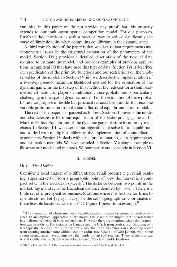
Consider a local market of a differentiated retail product (e.g., retail bank-ing, supermarkets). From a geographic point of view the market is a com-pact set C in the Euclidean space R2. The distance between two points in themarket, say a and b, is the Euclidean distance denoted by jja2bjj. There is afinite set of L pre-specified business locations where it is feasible for firms tooperate stores. Let fz1; z2; . . . ; zLg be the set of geographical coordinates ofthese feasible locations, where z‘ 2 C. Figure 1 presents an example.8

8 The assumption of a finite number of feasible locations is made for computational conven-ience. In an empirical application of the model, this assumption implies that the researcherhas to discretize the set of business locations. However, there are situations where this assump-tion can be realistic. For instance, in Canada and the U.S. leasing contracts at shopping cen-ters typically include a �radius restriction� clause that prohibits tenants in a shopping centerfrom opening another store within a certain radius (see Eckert and West [2006]). Also, somecountries and states have zoning laws that apply to �big box� retailers. These restrictions canbe sufficiently strict such that some retailers have only a few feasible locations.



Time is discrete. At time t the market is populated by a continuum ofconsumers. Each consumer is characterized by a geographical location orhome address z 2 C. The geographical distribution of consumers at period tis given by the absolute measure /tðzÞ such that

ÐC/tðdzÞ5Mt, where Mt is

the size of the market. This measure /t evolves over time according to adiscrete Markov process. Let X be the discrete set of possible functions /t.

9

There are I multi-store firms that can potentially operate in the market.We index firms by i and use !5f1; 2; . . . ; Ig to represent the set of firms.At the beginning of period t a firm�s network of stores is represented bythe vector nit5ðni1t; ni2t; . . . ; niLtÞ, where ni‘t is the number of stores thatfirm i operates in location ‘ at period t. For simplicity, we assume that afirm can have at most one store in a location, such that ni‘t 2 f0; 1g. Themodel can be easily generalized to the case with more than one store perlocation and firm.10 Overlapping of stores from different firms at the samelocation is allowed. In Section II(vii), we present an extension of the modelwhere business space is scarce in some locations such that there is a maxi-mum number of stores that can operate in each of these locations. Thespatial market structure at period t is represented by the vectornt5 n1t; n2t; . . . ; nItð Þ 2 f0; 1gIL. A store in this market is identified by apair ði; ‘Þ where i represents the firm, and ‘ identifies the location.

Every period t, firms observe the spatial market structure nt, the state ofthe demand /t, and some location and firm specific shocks in costs whichare private information of each firm. Given this information, incumbentfirms compete in prices. Prices can vary over stores within the same firm.

Figure 1Market and Feasible Business Locations (represented with �)

9 A market where the spatial distribution of consumers is constant over time (i.e., /tðzÞ5/ðzÞfor any z 2 C) is a particular case of our model.

10 In our model, two stores of the same firm and at the same location are perfect substitutes.Therefore, a firm will never find it optimal to have more than one store at the same location.However, it is straightforward to extend our logit demand model to allow for horizontal dif-ferentiation between stores with the same firm and location, i.e., the consumer-specificextreme value type 1 variables should vary across stores within a firm location.



This spatial Bertrand game is static because current prices do not have anyeffect on future demand or profits. Furthermore, private informationshocks affect fixed operating costs and entry costs but not the demand orvariable costs. Therefore, these shocks do not have any influence on equi-librium prices. The resulting Bertrand prices determine equilibrium variableprofits for each firm i at period t. At the end of period t, firms decidesimultaneously their network of stores for the next period. This choice isdynamic because of partial irreversibility in the decision to open a newstore, i.e., sunk costs. Firms are allowed to open or close at most one storeper period. Exogenous changes in the spatial distribution of demand (i.e.,changes in /t) and firms� location specific shocks generate entry and exitat different locations and changes over time in the spatial market structure.Firms may grow (or decline) over time expanding (contracting) their net-work of stores, and possibly become a dominant player (or exit from themarket). The details of this model are presented in Sections II(ii) to II(vi).In Section II(vii) we present several extensions of our basic framework.

Some assumptions about the basic structure of the model deserve furtherexplanation. First, while our model of entry-exit and store location isdynamic, we assume that the model of price competition is static. Thisimplies that there are no dynamics in demand, such as durable or storableproducts and consumer switching costs, or in variables costs, such as learn-ing by doing/selling, menu costs, or firm inventories. This structure of themodel follows the framework in Ericson and Pakes [1995] and Pakes andMcGuire [1994], as well as most of the recent literature on empiricaldynamic games of oligopoly competition (see Aguirregabiria and Nevo[2013]). An important reason for using this structure is convenience in thecharacterization and computation of an equilibrium. However, we alsobelieve that this structure is realistic for many retail industries, especially ifthe analysis is not particularly focused on the short-run dynamics ofprices.11 Second, our model allows for firms� private information in thedynamic game but assumes complete information in the static pricing game.We admit that allowing for private information in both games would bemore realistic. Our assumption of complete information in the pricing gameis mainly for convenience and it follows most of the empirical IO literatureon models of price competition in differentiated product industries. While itis relatively simple to characterize and compute a Bayesian Nash Equilib-rium in a discrete choice game of incomplete information (like a model ofmarket entry-exit), it is substantially more complicated in games where

11 Sales promotions and price dynamics related to storable products (Hendel and Nevo[2006]), or to firm inventories (Aguirregabiria [1999]) tend to occur at relatively high time fre-quencies. Our model of price competition can be interpreted in terms of firms� competition inaverage prices over a quarter or a year.



players� decisions are continuous variables, and even more if the decision isa vector of prices at each/store location, as in our pricing game.12

II(ii). Consumer Behavior

The model of consumer demand that we present here builds on De Palmaet al. [1985]. We extend their model in two dimensions. First, we incorpo-rate vertical differentiation (i.e., they assume that firms have the same qual-ities xi). And second, geographic location in our model has twodimensions while they consider a linear city.

A consumer is fully characterized by a pair ðz; vÞ, where z is her locationin geographic space or home address, and v 2 R

IL is a vector representingher idiosyncratic preferences over all possible stores. Consumer behavior isstatic and demand is unitary. At every period t, consumers know all activestores with their respective locations and prices. A consumer decideswhether to buy or not a unit of the good and from which store to buy it.The indirect utility of consumer ðz; vÞ patronizing store ði; ‘Þ at time t is:

ui‘t5xi‘2pi‘t2sgðjjz2z‘jjÞ1vi‘(1)

xi‘ is the quality of the product offered by retail chain i that, in principle,may vary exogenously across locations. All consumers agree on this mea-sure. pi‘t is the mill price charged by store ði; ‘Þ at time t. The terms gðjjz2z‘jjÞ represents consumer�s transportation costs, where s is the unittransportation cost and jjz2z‘jj is the Euclidean distance between the con-sumer�s address and the store, and g :ð Þ is a continuous and increasing func-tion.13 Finally, vi‘ captures consumer idiosyncratic preferences for storeði; ‘Þ. The utility of the outside alternative (i.e., not purchasing the good) isnormalized to zero.

A consumer purchases a unit of the good at store ði; ‘Þ if and only if ui‘t

� 0 and ui‘t � ui0‘0t for any other store ði0; ‘0Þ. To obtain the aggregatedemand at each store we have to integrate individual demands over the dis-tribution of ðz; vÞ. We assume that v is independent of z and it has a type 1extreme value distribution with dispersion parameter l. The parameter lmeasures the importance of horizontal product differentiation, other thanspatial differentiation. Integrating over v we obtain the local demand forstore i; ‘ð Þ from consumers at location z:

12 In a discrete choice game of incomplete information, a player�s strategy can be repre-sented as a vector of probabilities in the simplex. In contrast, in a continuous decision game ofincomplete information, a player�s strategy is a multivariate continuous function, which is asubstantially more complex object. Most applications of continuous decision games of incom-plete information have concentrated in relatively simple one-dimension strategies such as auc-tions, or price competition in homogeneous product industries.

13 The gð:Þ function can be linear, concave, or convex. As in the standard Hotelling modelof store location, if this function is convex, then the equilibrium of the model incorporates aconsumer transportation cost motive for the agglomeration of stores.



ri‘ðz; nt; ptÞ5ni‘t exp fðxi‘2pi‘t2sgðjjz2z‘jjÞÞ=lg

11XI

i051

XL

‘051

ni0‘0t exp fðxi0‘02pi0‘0t2sgðjjz2z‘0 jjÞÞ=lg(2)

Integrating these local demands over the spatial distribution of consumerswe obtain the aggregate demand for store ði; ‘Þ at time t:

si‘ðnt; pt;/tÞ5ðC

ri‘ðz; nt; ptÞ/tðdzÞ(3)

Consumers� substitution patterns depend directly on the distance func-tion jjz2z‘jj, so that a store competes more fiercely against closer stores.Stores� market areas are overlapping because of the unobserved heterogene-ity of consumers, v. Therefore a store serves consumers from all corners ofthe city C, but more so the nearby patronage. Stores will always face a posi-tive demand and can adjust prices without facing a perfectly elasticdemand. Firms face the trade-off between strategic and market shareeffects. As stores locate closer to each other, the more intense price compe-tition acts as a centrifugal force of dispersion (strategic effect). At the sametime, firms wish to locate where transportation costs are minimum, whichacts as a centripetal force of agglomeration (market share effect). An equi-librium spatial market structure would balance these forces, along with theeffect of own-firm stores cannibalization.

We note the importance of the parameters l and s that capture productdifferentiation. As l! 0 the degree of non-spatial horizontal product dif-ferentiation becomes small and every consumer shops at the store with thelowest full price from her location (i.e., quality-adjusted mill price plustransportation costs). At the limit we would observe market areas definedas Voronoi graphs (or Thiessen polygons) with well defined market borders(see Eaton and Lipsey [1975], or Tabuchi [1994], among others). Transpor-tation costs increase the importance of location, serve as a shield for mar-ket power and create incentives for firm dispersion.14

II(iii). Price Competition

For notational simplicity we omit the time subindex in this subsection.Every period firms compete in prices taking as given their network ofstores, the state of the demand, and variable costs. Firms may charge dif-ferent prices at different stores. This price competition is a game of

14 Besides computing equilbrium prices, our Bertrand algorithm computes demand priceelasticities for each location and store at these prices. These elasticities help the researcher bet-ter understand what the actual market areas are in geographic space. The detection of the rele-vant geographical market area has long been debated among antitrust authorities (see Willig[1991] and Baker [1997]).



complete information. In this game, every firm knows the current networksof stores, the demand system, and the unit costs of all active stores. A firmvariable profit function is:

Riðn; p;/Þ5XL

‘51

pi‘2ci‘ð Þsi‘ðn; p;/Þ(4)

ci‘ is the unit variable cost of firm i at location ‘ which is assumed constantover time. Each firm maximizes its variable profit by choosing its best-response vector of prices. The best response of firm i can be characterizedby the first-order condition for each price pi‘:

si‘1 pi‘2ci‘ð Þ @si‘

@pi‘1X‘0 6¼‘

pi‘02ci‘0ð Þ @si‘0

@pi‘50(5)

The first two terms are the price and quantity effects of pi‘ on the profit atits own store ði; ‘Þ, while the last term is the quantity effect of pi‘ on all otherstores of firm i. This last term is zero for a single-store firm. For a multi-store firm, this term captures how the pricing decision of the firm internal-izes the cannibalization effect among its own stores. In our demand system,stores of a same firm are gross substitutes (i.e., @si‘0=@pi‘ > 0 for ‘0 6¼ ‘) andtherefore the third term is always positive. Given that @si‘=@pi‘ < 0, we havethat, ceteris paribus, a multi-store firm will offer higher prices than a single-store firm. The firm knows that by reducing the price in one of its storesthere is a business stealing effect on its other stores.15

Let p and s pð Þ be vectors with dimension IL31 of prices and demands,respectively, for every store. Following Berry [1994] and Berry et al. [1995],we define a square matrix K pð Þ of dimension IL3IL with elements:

Kj‘0

i‘ 52@sj‘0

@pi‘if j5i

0 otherwise

8><>:(6)

We can write the entire system of best-response equations in vector form ass pð Þ2K pð Þ � p2cð Þ50, or what is equivalent:

p5c1K pð Þ21 � s pð Þ(7)

where c is the IL31 vector of unit costs. A spatial Nash-Bertrand equilib-rium is then a vector p� that solves the fixed-point mapping (7). Given our

15 Of course, there are cost factors (e.g., economies of scale and density) that can make pri-ces of multi-store firms smaller than prices of single-store firms. The effect that we illustrate inequation (5) is only the cannibalization effect.



assumptions on the distribution of consumer taste heterogeneity v, themappings s pð Þ and K pð Þ are continuously differentiable. Furthermore, it ispossible to show that, for every firm i and location ‘, an equilibrium pricep�i‘ in this game is always greater than or equal to the constant marginalcost ci‘ and smaller than or equal to the equilibrium price at store ði; ‘Þwhen firm i is a monopolist with stores at every location in the city. There-fore, the vector of prices p belongs to a compact set: p belongs to the IL-dimension rectangle (i.e., lattice) < c; pMon >, where pMon is the vector ofmonopoly prices for each firm-location. By Brower�s fixed-point theorem,a Nash-Bertrand equilibrium exists.

The equilibrium is not necessarily unique. Multiplicity of equilibria maybe a problem when we use the model for comparative statics or to evaluatethe effects of public policies. A possible way of dealing with multiplicity ofequilibria is to impose an equilibrium selection mechanism, i.e., a criterionthat selects a specific type of equilibrium such that when we do compara-tive statics the same equilibrium type is always selected. To implement anequilibrium selection mechanism in practice, we need an algorithm thatcan find the specific type of equilibrium for any possible specification ofthe primitives of the model. We describe here an algorithm with these fea-tures that exploits the supermodularity of this Bertrand game.

The algorithm is based on Topkis [1979], [1998] and Echenique [2007].Following Vives [1999] (page 32), our Bertrand game is smooth supermod-ular if it satisfies the following conditions: (i) the space of prices is a lattice;(ii) the profit function Rið:Þ is twice continuously differentiable in prices;(iii) @2Ri=@pi‘@pjm � 0 for any i 6¼ j and any pair of locations ‘ and m; and(iv) @2Ri=@pi‘@pim � 0 for any ‘ 6¼ m. As mentioned above, conditions(i) and (ii) are satisfied in this pricing game because p belongs to the lattice< c; pMon > and the revenue function is twice continuously differentiablewithin that set. A sufficient (but not necessary) condition for (iii) and (iv)to hold is that the local market shares ri‘ðz; pÞ are never larger than a halfwithin the set < c; pMon >.16 More generally, this Bertrand game is smooth

16 For condition (iii) we have that for i 6¼ j:

@2Ri

@pi‘@pjm5

@si‘

@pjm

� �1 pi‘2ci‘ð Þ @2si‘

@pi‘@pjm

� �1X‘0 6¼‘

pi‘02ci‘0ð Þ @2si‘0

@pi‘@pjm

24

35

The first and the third terms in brackets are always positive. For the second term, we havethat: @2si‘=@pi‘@pjm5l21

Ð@ri‘ðzÞ=@pjm 122ri‘ðzÞð Þ/ðdzÞ. Since @ri‘ðzÞ=@pjm > 0, a sufficient

condition for this second term to be positive is that, for any location z 2 C, the local marketshares ri‘ðzÞ are smaller than 1/2. This condition holds when qualities are not too large andthe degree of horizontal product differentiation l is not too small relative to transportationcosts. However, it is clear that this sufficient condition is far from being necessary. Local mar-ket shares greater than 1/2 are perfectly compatible with a positive value for @2si‘=@pi‘@pjm.Furthermore, it is clear that the cross-price second derivative of the profit function can be



supermodular if quality differences between firms are not too large and thedegree of horizontal product differentiation (l) is not too small relative totransportation costs (s).

The following Lemma is a straightforward application to our Bertrandgame of a general result by Topkis [1979] for supermodular games. TheLemma establishes a simple algorithm to obtain the equilibria with thesmallest and with the largest prices, respectively.

Lemma. Define the best response mapping in vector form, bðpÞ � c1K pð Þ21s pð Þ. Consider the following algorithm (best response function iter-ation): start with an initial vector of prices p0; at iteration k � 1,pk5bðpk21Þ; stop when pk5pk21. If the game is supermodular then:

i. if we start with p05c, then the algorithm stops at the Nash-Bertrandequilibrium with smallest prices, plow;

ii. if we start with p05pMon, then the algorithm stops at the Nash-Bertrand equilibrium with largest prices, phigh.

Topkis [1979] proved this Lemma for supermodular games, and Topkis[1998] extended the result to a more general class of games with strategiccomplementarities (GSC). The proof is relatively simple. If the game issupermodular, then the best response mapping bðpÞ is monotonicallyincreasing. This implies that bðcÞ � c, and b2ðcÞ � bðbðcÞÞ � c,. . ., andbkðcÞ � bk21ðcÞ, such that iterating in bð:Þ generates a monotonicallyincreasing sequence in the space of prices < c; pMon >. But the space of pri-ces is compact, so there must be an iteration such that bkðcÞ5bk21ðcÞ, andthis implies that bkðcÞ is a Nash-Bertrand equilibrium. Let plow be thatequilibrium, and let p� be another equilibrium of the game. Since p� � cand the best response mapping is monotonically increasing, we have thatplow5 bkðcÞ � bkðp�Þ 5 p� for any equilibrium p�. Therefore, plow is theequilibrium with smallest prices. Similarly, if we initialize the algorithmwith p05pMon, we generate a monotonically increasing sequence, bðpMonÞ� b2ðpMonÞ � . . . � bkðpMonÞ that should converge in the compact space of

positive when @2si‘=@pi‘@pjm is negative just because the other two terms can be larger in abso-lute value. For condition (iv) we have that for ‘ 6¼ m:

@2Ri

@pi‘@pim5

@si‘

@pim1@sim

@pi‘

� �1 pi‘2ci‘ð Þ @2si‘

@pi‘@pim1 pim2cimð Þ @2sim

@pi‘@pim

� �

1X

‘0 6¼f‘;mgpi‘02ci‘0ð Þ @2si‘0

@pi‘@pim

24

35

Again, the first and the third terms in brackets are always positive. The second term is alsopositive under the same conditions as mentioned above.



prices. Let phigh be that equilibrium. Since any equilibrium p� is such thatp� � pMon, we have that phigh5 bkðpMonÞ � bkðp�Þ 5 p� for any equilibriump�. Therefore, phigh is the equilibrium with largest prices.17

Based on this Lemma, we can use Topkis algorithm to select always thesame type of Nash-Bertrand equilibrium, e.g., the equilibrium with mini-mum prices. The two extremal equilibria coincide with the Pareto best andthe Pareto worst equilibria from the point of view of firms (see Vives[1999], page 152). In the numerical examples in Section V, we use Topkisalgorithm to select the Nash-Bertrand equilibrium with smallest prices: theworst equilibria from the point of view of firms.18

Let p� n;/ð Þ be the vector of equilibrium prices associated with a valuen;/ð Þ of the state variables. Solving this vector into the variable profit

function one obtains the equilibrium variable profit function:

R�i n;/ð Þ � Riðn; p� n;/ð Þ;/Þ(8)

II(iv). Dynamic Game

At the end of period t firms simultaneously choose their network of storesnt11 with an understanding that they will affect their variable profits atfuture periods. We model the choice of store location as a game of incom-plete information, so that each firm i has to form beliefs about other firms�choices of networks. More specifically, there are components of the entrycosts and exit values of a store which are firm-specific and private informa-tion. There are two main reasons why we include incomplete informationin our model. First, as shown by Doraszelski and Satterthwaite [2010], inthe Ericson-Pakes complete-information model of industry dynamics anequilibrium in pure strategies does not necessarily exist. Doraszelski andSatterthwaite also show that the introduction of private information varia-bles with continuous distribution function and large support guaranteesthe existence of an equilibrium in this class of games of industry dynamics.Second, the recent literature on estimation of dynamic games has also con-sidered games of incomplete information because these variables are con-venient sources of unobserved heterogeneity from the point of view of the

17 See also Echenique [2007], who has developed an efficient algorithm to find all the equili-bria in GSC. The implementation of Echenique�s algorithm is relatively simple. Once we haveobtained the lowest equilibrium, plow, we can define a new game with the same payoff func-tions as our game but where the set of feasible prices is the lattice < plow1d; pMon >, and d > 0is a small constant. Then, we can apply Topkis algorithm to obtain the lowest equilibrium ofthis game. It is straightforward to show that this equilibrium is the one with the second lowestprices in our Bertrand game. We can proceed in this way to obtain a sequence of equilibriasorted by the value of prices. The algorithm continues until an iteration K where the K-lowestequilibrium is exactly the highest equilibrium, phigh.

18 We can also use the Lemma to check for multiplicity of equilibria. If the smallest equilib-rium coincides with the largest equilibrium, then the equilibrium is unique.



researcher (see Aguirregabiria and Mira [2007], or Pakes, Ostrovsky andBerry [2007]).

We assume that a firm may open or close at most one store per period.Given that we can make the frequency of firms� decisions arbitrarily high,this is a plausible assumption that reduces significantly the cost of comput-ing an equilibrium in this model. Let ait be the decision of firm i at periodt such that: ait5‘1 represents the decision to open a new store at location‘; ait5‘2 means that a store at location ‘ is closed; and ait 5 0 meansthe firm chooses to do nothing. Therefore, the choice set isA5f0; ‘1; ‘2 : ‘51; 2; . . . ;Lg. Some of the choice alternatives in A are notfeasible for a firm given its current network nit. In particular, a firm cannot close a store in a submarket where it has no stores, and it cannot opena new store in a location where it already has a store. The set of feasiblechoices for firm i at period t is denoted AðnitÞ such that AðnitÞ5 f0g[f‘1 : ni‘t50g[ f‘2 : ni‘t51g. Note that this choice set has exactly L 1 1choice alternatives.

We represent the transition rule of market structure as nt115nt11½at�,where 1½at� is a IL31 vector such that its ði; ‘Þ-element is equal to 1 1when ait5‘1, to 21 when ait5‘2, and to zero otherwise. That is, the ði; ‘Þ-element of 1½at� is equal to 1fait5‘1g21fait5‘2g, where 1f:g is the indica-tor function.

II(v). Specification of the Profit Function

Firm i�s current profit is:

Pit 5 R�i nt;/tð Þ2FCit2ECit1EVit(9)

FCit is the fixed cost of operating all the stores of firm i. ECit is the entryor set-up cost of a new store. And EVit is the exit value of closing a store.Fixed operating costs depend on the number of stores but also on theirlocation.

FCit 5XL

‘51

hFCi‘ ni‘t(10)

hFCi‘ is the fixed cost of operating a store in submarket ‘. In Section II(vii),

we extend this basic specification to incorporate economies of scale anddensity in the fixed cost of a retail chain. The specification of entry cost is:

ECit 5XL

‘51

1fait5‘1g hECi‘ 1eEC

i‘t

� �(11)



hECi‘ is the entry cost at location ‘. The variable eEC

i‘t represents a firm andlocation specific component of the entry cost. This idiosyncratic shock isprivate information of firm i. The specification of the exit value is:

EVit 5XL

‘51

1fait5‘2g hEVi‘ 1eEV

i‘t

� �(12)

hEVi‘ is the scrapping or exit value of a store in location ‘. The variable eEV

i‘tis a firm and location specific shock in the exit value of a store.

The vector of private information variables for firm i at period t iseit5feEC

i‘t ; eEVi‘t : ‘51; 2; . . . ;Lg. We make two assumptions on its distribu-

tion. First, we assume that eit is independent of demand conditions /t, andindependently distributed across firms and over time. Independence acrossfirms implies that a firm cannot learn about other firms� e�s by using itsown private information. And independence over time means that a firmcannot use other firms� histories of previous decisions to infer their currente�s. These assumptions simplify significantly the definition and the compu-tation of an equilibrium in this dynamic game. Second, we assume that eit

has a cumulative distribution function Gið:Þ that is strictly increasing andcontinuously differentiable with respect to the Lebesgue measure in R

2L.These two assumptions allow for a broad range of specifications for theeit�s, including spatially correlated shocks.

It will be convenient to distinguish two additive components in the cur-rent profit function:

Pit5pi ait; nt;/tð Þ1eitðaitÞ(13)

where pi ait; ntð Þ is the current profit function excluding the private infor-mation variables, and eitðaitÞ represents the private information shock asso-ciated with action ait.

II(vi). Markov Perfect Equilibrium

We consider that a firm�s strategy depends only on its payoff relevant statevariables ðnt;/t; eitÞ. For the sake of notational simplicity, hereinafter weomit the state of the demand /t as an argument of the different functions.Let a � faiðnt; eitÞ : i 2 !g be a set of strategy functions, one for each firm,such that ai is a function from f0; 1gIL

3R2L into A. Given a set of strategy

functions a, we can define a value function V ai ðnt; eitÞ that represents the

value of firm i given that the other firms behave according to their strategyfunctions in a and firm i responds optimally. The value function V a

i is theunique solution of the following Bellman equation:



V ai ðnt; eitÞ5 max

ait2AðnitÞva

i ðait; ntÞ1eitðaitÞ� �

(14)

where the functions vai ðait; ntÞ are choice specific value functions which are

defined as:

vai ðait; ntÞ �pi ait; ntð Þ1b

ðV a

i nt11½ait; a2iðnt; e2itÞ�; ei;t11

� �

3dGiðei;t11ÞYj 6¼i

dGjðejtÞ" #(15)

Similarly, we can define firm i�s best response function, aBRi ðnt; eit; a2iÞ, as:

aBRi ðnt; eit; a2iÞ5 arg max

ait2AðnitÞva

i ðait; ntÞ1eitðaitÞ� �

(16)

A Markov perfect equilibrium (MPE) in this game is a set of strategy func-tions such that each firm�s strategy maximizes the value of the firm foreach possible ðnt; eitÞ and taking other firms� strategies as given.

Definition. A set of strategy functions a� � fa�i ðnt; eitÞ : i 2 !g is an MPEif and only if for any firm i and any state ðnt; eitÞ we have that:

a�i ðnt; eitÞ5aBRi ðnt; eit; a

�2iÞ(17)

Next, we follow Aguirregabiria and Mira ([2007], pp. 7–13) to representan MPE as a fixed point in a space of choice probabilities. The algorithmthat we use to compute an equilibrium (in Section III(ii)) uses this repre-sentation. We start by defining three objects: conditional choice probabil-ities; integrated value function; and best response probability function.

Conditional choice probabilities (CCP�s). Given any set of strategy functionsa, we can define a set of conditional choice probabilities Pa � fPa

i ðaitjntÞ :i 2 !; ait 2 A; nt 2 f0; 1gILg such that

Pai ðaitjntÞ � Pr ðaiðnt; eitÞ5aitjntÞ5

ð1 aiðnt; eitÞ5aitf gdGiðeitÞ(18)

The probabilities in Pa represent firms� expected behavior, from the pointof view of the competitors, when firms follow their respective strategiesin a. Given that ait and nt are discrete variables with finite support, Pa

is a vector in an Euclidean space of finite dimension.19 More precisely,

19 Note that we have assumed that /t can take only a finite number of values. Therefore,Pa

i ðaitjnt;/tÞ also belongs to a finite-dimension Euclidean space.



Pa 2 ½0; 1�D where D5I � L � 2IL is the number of free probabilities in thevector Pa.

Define the integrated value function �V ai ðntÞ �

ÐV a

i ðnt; eitÞdGiðeitÞ. Apply-ing the definitions of CCP�s and integrated value function to the Bellmanequation in (14)-(15) we get the following integrated Bellman equation:

�V ai ðntÞ5

ðmax

ait

pi ait; ntð Þ1eitðaitÞf

1bXa2it

�V ai nt11½ait; a2it�ð Þ

Yj 6¼i

Paj ðajtjntÞ

" #)dGiðeitÞ

(19)

The integrated value function �V ai is the unique fixed point of this Bellman

equation. Notice that the fixed point mapping that defines �V ai depends on

firms� strategies only through the vector of choice probabilities Pa. Toemphasize this point and to define an MPE in probability space, we changethe notation slightly and use the symbol �V P

i instead of �V ai to denote the

integrated value function. For the same reason, we use vPi ðait; ntÞ to repre-

sent the choice-specific value functions, which can be written as:

vPi ðait; ntÞ � pi ait; ntð Þ1b

Xa2it

�V Pi nt11½ait; a2it�ð Þ

Yj 6¼i

Paj ðajtjntÞ

" #(20)

Given these value functions, we can re-write the best response function as:aBR

i ðnt; eit;PÞ5arg max ait2AðnitÞfvPi ðait; ntÞ1eitðaitÞg. Note that we have

replaced a2i by P as an argument in the best response function. This isbecause CCP�s contain all the information about competitors� strategiesthat a firm needs to construct its best response.

The best response probability function, Wiðaitjnt;PÞ, is the probabilitythat action ait is firm i�s best response given that the state of the market isnt and the other firms behave according to their choice probabilities in P. Itis the best response function aBR

i integrated over the distribution of privateinformation variables.

Wiðaitjnt;PÞ �ð1 ait5arg max

a2AðnitÞvP

i ða; ntÞ1eitðaÞ� ��

dGiðeitÞ(21)

This function maps CCP�s into CCP�s. The best response probability func-tion in vector form is WðPÞ5fWiðaitjnt;PÞ : ði; ait; ntÞ 2 !3A3f0; 1gILg.

Let a� be a set of MPE strategies and let P� be the vector of CCP�s asso-ciated to a�. Using the previous definitions it is simple to verify that P�

should be a fixed point of the mapping W. Inversely, let P� be a fixed pointof the mapping W, and define the set of strategy functions a� with



a�i ðnt; eitÞ5arg max aitfvP�i ðait; ntÞ1eitðaitÞg. Then, it is also simple to verify

that a� is an MPE (see Aguirregabiria and Mira [2007], for further details).Therefore, we can represent any MPE in this model as a fixed point of thebest response probability mapping. Equilibrium probabilities solve thecoupled fixed-point problems defined by equations (19), (20) and (21).Given a vector of probabilities P, we obtain value functions �V P

i as solutionsof the I Bellman equations in (19), and given these value functions, weobtain best response probabilities using (21).

Given this representation of an equilibrium, the proof of existence of anMPE is a straightforward application of Brower�s theorem. The distribu-tion Gið:Þ has support over the entire R

2L and it is continuous and strictlyincreasing with respect to every argument. This implies that the fixed-pointmapping W is continuous on the compact set ½0; 1�D. Thus, by Brower�stheorem, an equilibrium exits.

Example. The functional forms of the integrated Bellman equation and ofthe best response probability mapping depend on the distribution of the pri-vate information variables. A special case in which these functions have closeform expressions is when the private information variables have a type1 extreme value distribution. Suppose that the private information shocks feitðaÞ : a 2 Ag are independently and identically distributed over ði; t; aÞ withtype 1 extreme value distribution. Then, the integrated Bellman equation is:

�V Pi ðntÞ5log

Xait2AðnitÞ

exp vPi ðait; ntÞ

� �0@

1A(22)

And the best response probability function is:

Wiðaitjnt;PÞ5exp vP

i ðait; ntÞ� �

Pa2AðnitÞ exp vP

i ða; ntÞ� �(23)

The iid extreme value distribution is restrictive because it implies no spatialcorrelation between private information shocks. However, it is very conven-ient from a computational point of view because it avoids numerical inte-gration over the space of eit. �

This dynamic game can have multiple equilibria. This is an issue whenwe use this model for comparative statics. In principle, a researcher may bewilling to deal with multiplicity by imposing an equilibrium selectionmechanism such that, for different values of the model parameters, thesame equilibrium type is always selected. We illustrated in Section II(iii)how imposing an equilibrium selection mechanism is relatively simple in



static supermodular games. Unfortunately, it is generally difficult to estab-lish supermodularity in dynamic games.20

To deal with multiple equilibria in the dynamic game, we use differentapproaches when estimating the model and when making counterfactualexperiments. In Section IV, we describe different estimation methods thatdo not require solving for an equilibrium of the dynamic game and thatcan deal with multiplicity at the estimation stage. In Section III(iii), wepresent a computationally simple homotopy method to deal with multiplic-ity of equilibria in the implementation of counterfactual experiments. Themethod involves the computation, or approximation, of only two equili-bria, one under the factual scenario and other under the counterfactual.

II(vii). Extensions of the Benchmark Model

(a) Positive spillover effects from other stores. In order to reduce theirsearching/shopping costs, consumers may be attracted to locations withmultiple stores selling the same differentiated product. This argumentimplicitly assumes that when consumers decide which location to visit theyhave some uncertainty about product availability (stockouts) or quality ofservice at stores and this uncertainty disappears only when the consumervisits the store. We do not model explicitly this consumer uncertainty.Instead, we extend our specification of consumer utility by including a newterm that accounts for a positive spillover effect from the presence of otherstores. The indirect utility of consumer ðz; vÞ patronizing store ði; ‘Þ is:

ui‘5xi‘1dhXj 6¼i

nj‘

!2pi‘2sgðjjz2z‘jjÞ1vi‘(24)

where d is a positive parameter, hð:Þ is an increasing function, andP

j 6¼i nj‘

is the number of stores at location ‘ from firms other than i. This extensionof the model does not have any effect on the basic structure of the demandmodel and of the Bertrand equilibrium. All the results above remain byonly replacing xi‘ with x�i‘, where x�i‘ � xi‘1d hð

Pj 6¼i nj‘Þ. However, this

extension can have substantial effects on the spatial configuration of storesin equilibrium, and on the relationship between equilibrium prices and thenumber of stores in a location.

In our benchmark model of price competition, the number of stores in alocation only has a competition effect in the sense that, ceteris paribus, pricesare lower in locations with more stores. In this extended model with spill-overs, the number of stores in a location still has a competition effect, but it

20 Curtat [1996] provides a useful overview of the problem. More recently, Bernstein andK€ok [2009] have obtained conditions for the supermodularity of a dynamic game of innova-tion and cost reduction in assembly networks.



also has a positive effect on prices due to the increase in consumer traffic.The net effect on prices can be either positive or negative depending on therelative magnitude of the spillover parameter d and the parameter l thatrepresents the degree of (non-spatial) horizontal product differentiation.

Our benchmark dynamic model of store location includes some featuresthat can generate agglomeration of stores in some locations, e.g., minimiza-tion of consumer transportation costs if function gð:Þ is convex; or loca-tions with high (low) values of the amenities xi‘ (costs). The extendedmodel with positive spillover effects introduces an additional centripetalforce of store agglomeration.

(b) Store experience increases quality. It is well known in the empiricalIO literature that firms or stores that have been longer in the market aremore productive and have larger market shares, on average, than youngerstores. There are multiple (not mutually exclusive) explanations for thisempirical evidence, e.g., dynamic selection, active or passive learning. Herewe present a simple extension of our benchmark model that incorporatesstore passive learning. Stores that stay active accumulate experience, andthis experience has a positive effect on the service quality the store providesto customers. The specification of consumer utility is:

ui‘t5xi‘1ck ei‘tð Þ2pi‘t2sgðjjz2z‘jjÞ1vi‘(25)

where c is a positive parameter that captures the magnitude of the experi-ence effect on quality, k :ð Þ is an increasing function, and ei‘t is a discretevariable that measures the experience of a store at period t, e.g., a dummyvariable that is equal to zero if the store is brand new and equal to one oth-erwise; or the number of consecutive periods that the store has been activein the market, with a maximum value �e.

This extension has no implications on the basic structure of the Bertrandequilibrium model and the computation of an equilibrium, but it has rele-vant implications on its predictions. The extended model predicts that, inequilibrium, younger stores charge lower prices. This extension implies amore substantial modification in the structure of the dynamic game. Now,the vector of endogenous state variables describing retail chain networks isfnt; etg where et � fei‘t : i 2 !; ‘51; 2; . . . ;Lg is the vector of store experi-ences. Similar to nt, the vector et has also a deterministic transition ruleconditional on firms� entry-exit decisions. Otherwise, the description of aMarkov Perfect Equilibrium does not change. However, this extension canhave substantial implications on the predictions of the dynamic game. Thepositive effect of experience on store quality introduces a first-moveradvantage, creates incentives for �early� entry, and discourages entry in loca-tions with experienced incumbents.



(c) Economies of scale and density at the chain level. The specification offixed costs can be extended to take into account that the fixed cost of oper-ating a network of stores may depend on the number of stores (e.g., econo-mies of scale) and on the distance between the stores (e.g., economies ofdensity). Economies of density are spatial scope economies enjoyed byclustered stores belonging to the same firm, in the sense that the closer thestores of a firm are to each other in space, the more scope economies thereare. For example, such density economies may include reduced distributioncosts, easier product quality inspection and employee monitoring, andsharing of advertising, inventory, and personnel among same-firm stores.The recent empirical IO literature on retail chains has emphasized theimportance of these economies of scale and density (Holmes [2011], Jia[2008], Nishida [2014]). Here we present an extended version of our bench-mark model that includes economies of density in fixed costs using a speci-fication similar to Jia [2008]. Other specifications are possible, as well asincorporating similar network effects in other components of the modelsuch as variable costs, entry costs, or even consumer demand.

The fixed cost of operating store ði; ‘Þ is:

hFCi‘ ni‘t2

hED

2

X‘0 6¼‘

ni‘0t

jjz‘02z‘jj(26)

where hED is a parameter that represents the magnitude of the economies ofdensity. The effect on this fixed cost of stores of the same firm at other locationsis weighted by the inverse of the distance to location ‘. This term is multipliedby one-half to avoid double counting in the total fixed cost of the retail chain.

This extension does not alter the basic structure of the dynamic game, andit does not have any implication on the pricing game (i.e., conditional onmarket structure nt, equilibrium prices are the same as in the benchmarkmodel). However, economies of density can have very substantial implicationson the predictions of the model. For obvious reasons, spatial agglomerationof stores of the same chain should be stronger with economies of density. Itseems plausible that this extension can generate an equilibrium with the fla-vour of spatial entry deterrence, i.e., if chain A is an incumbent in location ‘,then this reduces the probability that chain B opens a store in locations closeto ‘. This implies that store agglomeration becomes stronger for stores of thesame chain but weaker for stores of different chains. Moreover, economies ofdensity could potentially cause such within-firm agglomeration of stores evenif there is no spatial entry deterrence motive. For example, under densityeconomies a firm with a store in location ‘ would likely prefer to open a newstore in a location that is near location ‘ (instead of in a similar but more dis-tant location) simply because its overall fixed operating costs would be lowerdue to the density economies.



(d) Scarce business space. Some business locations are unique in thesense that they offer a limited number of slots for retail stores. For example,it is not unusual for open-air �strip malls� to have a small number of lotsthat can accommodate large retailers such as supermarkets or departmentstores. Such restriction can be even stronger if one considers older and/ordenser cities. Here we present an extension of our benchmark model thatincorporates a simple version of this feature. Suppose that a location ‘ canaccommodate a maximum of N‘ stores. The values N‘ at different locationsare common knowledge to firms. However, the incomplete informationnature of our dynamic game implies that, when firms make their entry-exitdecisions, they do not know how many other firms want to operate a storein a location. Therefore, we distinguish between firms �applications� forstore entry and the actual realization of entry decisions.

Let a�it 2 AðnitÞ be the decision of firm i at period t, where the set AðnitÞhas exactly the same definition as in the benchmark model. However, a�itrepresents an �application� and not necessarily the actual opening-closingof stores of the firm. Let ait be the variable that represents the actualchange in the store network of firm i, such that nit115nit11faitg as in thebenchmark model. We consider the following relationship between thedecisions/applications fa�itg and the actual realizations of store entry-exitfaitg. First, if the application is for closing an existing store (i.e.,a�it5‘2 2 AðnitÞ) or for doing nothing (i.e., a�it50), then this application isrealized with probability one such that ait5a�it. Second, if the application isfor opening a new store (i.e., a�it5‘1 2 AðnitÞ), then this request is not auto-matically implemented and there is some uncertainty. Let Ninc

‘t11 be the totalnumber of incumbent stores in location ‘ at period t that decide to stay inthe market, i.e., Ninc

‘t11 �PI

i51 ni‘t 1fa�it 6¼ ‘2g. And let Nnew‘t11 be the num-

ber of new applicants for opening a store, i.e., Nnew‘t11 �

PIi51 1fa�it5‘1g.

The allocation of the N‘ slots follows two simple rules: (1) if there is notexcess demand for business slots at location ‘ (i.e., if Ninc

‘t111Nnew‘t11 � N‘),

then all the applications are accepted; and (2) if there is excess demand(i.e., if Ninc

‘t111Nnew‘t11 > N‘), then all the incumbents can keep their stores

with probability one and the new applicants enter into a lottery for theallocation of the remaining N‘2Ninc

‘t11 slots. Different lotteries may be con-sidered. The simplest one is a sequential lottery of each slot where all theapplicants have the same probability of winning a slot. Other lotteriesmight be considered to try to capture that firms may have different willing-ness to pay for a business slot.

This extension of the benchmark model introduces an additional sourceof uncertainty in the dynamic game. Firms� strategy functions and Condi-tional Choice Probabilities are defined in terms of the application decisionsfa�itg in a very similar way as in our benchmark model. The main differenceappears in the transition rule of store networks that becomes stochastic.



The implications of this new source of uncertainty on the predictions ofthe model are not obvious. Of course, the scarcity of business space shouldreduce entry and store agglomeration in some locations.

III. ALGORTHIMS FOR SOLUTION AND COMPARATIVE STATICS

III(i). Computation of a Nash-Bertrand equilibrium

To compute a Nash-Bertrand equilibrium of the static pricing game, weiterate in the best response function. More specifically, we use a Gauss-Seidel version of the algorithm that iterates in the best response mapping,such that players take turns in best-responding instead of jointly best-responding in each iteration. Topkis [1998] has shown that the Lemma thatwe have presented in Section II(iii) also applies to the Gauss-Seidel versionof the algorithm. In fact, Topkis shows that for supermodular games theGauss-Seidel algorithm is faster (see also Echenique [2007]).

For a given value of the state variables, we have defined the best responsemapping as b pð Þ � c1K pð Þ21 � s pð Þ. Let bðiÞ pð Þ be the elements of b pð Þassociated with the prices of firm i. Similarly, let pðiÞ be the elements of thevector p associated with firm i. To obtain the equilibrium with smallest pri-ces we initialize the algorithm with prices equal to marginal costs.

Step 0: Start with the vector of prices p0 such that p0ðiÞ5ci for any

i 2 !.Step 1: Compute aggregate demands s p0

� �and the matrix of partial

derivatives K p0� �

using quadrature integration (see below).Step 2 (Gauss-Seidel iteration): Starting with firm 1, obtain a new vec-

tor p1ð1Þ as p1

ð1Þ5bð1Þ p0� �

. Then, for firm 2, p1ð2Þ5bð2Þðp1

ð1Þ; p0ð2Þ; . . . ; p0

ðIÞÞ,and so on for firm i, p1

ðiÞ5bðiÞðp1ð1Þ; . . . ; p1

ði21Þ; p0ðiÞ; . . . ; p0

ðIÞÞ.Step 3: If jjp12p0jj is smaller than a pre-fixed small constant, then

p�5p1. Otherwise, proceed to step 1 with p05p1.

Once the price equilibrium is computed, we encode the equilibrium currentvariable profits of a firm given a particular state, R�i ðn;/Þ.

Given the logit assumption on the idiosyncratic tastes, the local demandshave the closed form expression in (2). However, to obtain the vector ofaggregate demands s pð Þ and the matrix of partial derivatives K pð Þ we haveto integrate local demands over consumers� addresses in the two-dimensional city C. We use a quadrature method with midpoint nodes(see Judd [1998], ch. 7). We first divide C into a pre-specified number ofmutually exclusive and adjacent rectangular cells, with each cell k having arepresentative node point z kð Þ in its center. For each location z in cell kwe approximate the local demand ri‘ðz; nt; ptÞ and the density /t zð Þ usingri‘ðz kð Þ; nt; ptÞ and /t z kð Þ

� �, respectively. Therefore, we calculate aggregate

demand for store ði; ‘Þ as:



si‘ðnt; pt;/tÞ5X

k

ri‘ðz kð Þ; nt; ptÞ/t z kð Þ� �

areaðkÞ(27)

where area(k) is the area of the rectangular cell k.

III(ii). Computation of an MPE

Consider the example where the private information variables are extremevalue distributed. A MPE is a vector of probabilities P� such thatP�5WðP�Þ, where the fixed-point mapping WðPÞ is fWiðaitjnt;PÞ : ði; ait; ntÞ2 !3AðnitÞ3f0; 1gILg with

Wiðaitjnt;PÞ

5

exp piðait; ntÞ1bXa2it

�V Pi ðnt11½ait; a2it�Þ

Yj 6¼i

PjðajtjntÞ" #( )

Xai2AðnitÞ

exp piðai; ntÞ1bXa2it

�V Pi ðnt11½ai; a2it�Þ

Yj 6¼i

PjðajtjntÞ" #( )

(28)

and the value function �V Pi solves the Bellman equation

�V Pi ðntÞ5 log

Xait2AðnitÞ

exp pi ait; ntð Þf

0@

1bXa2it

�V Pi nt11½ait; a2it�ð Þ

Yj 6¼i

PjðajtjntÞ" #)!

(29)

To obtain an MPE we iterate in the best response function W usingGauss-Seidel iterations. The algorithm proceeds as follows.

Step 0: Initialize the algorithm with a vector of probabilities P0.Step 1 [Value function]: Starting with firm 1, and given

P02;P

03; . . . ;P0

I

� �fixed, we obtain the value function �V P0

1 by applyingvalue function iterations in the Bellman equation (29).

Step 2 [Best response]: Given �V P0

1 , we use the best response probabil-ity mapping in (28) to obtain a new vector of CCP�s for firm 1:P1

15fW1ðaitjnt;P0Þg.Then, we proceed with firm 2. Given P1

1;P03; . . . ;P0

I

� �fixed, we obtain

the value function �VP1

1;P03;...;P

0Ið Þ

2 by using value function iterations in theBellman equation (29). Then, we update firm 2�s CCP�s asP1

25fW2ðaitjnt;P11;P

03; . . . ;P0

I Þg. We proceed in this way to update theCCP�s of the I firms.



Step 3: If jjP12P0jj is smaller than a pre-fixed small constant, thenP�5P1. Otherwise, proceed to step 1with P05P1.

The most serious burden for the computation of an equilibrium in ourmodel comes from the space-memory requirements.21 Value functions andchoice probabilities should be stored in high-speed memory because theyare required for value function iteration and for the calculation of bestresponse probabilities. Given that the vector of state variables nt is discrete,value functions and choice probability functions can be described as vectors

in Euclidean spaces: i.e., �V Pi 2 R

2ILand P 2 ½0; 1�ILð2

ILÞ. In applicationswith many locations (or firms), the dimension of these Euclidean spacescan be very large. For instance, in a duopoly model with 40 locations wehave that 2IL ’ 1012. This magnitude of memory space is rarely available.

There are two general approaches to deal with this computational issue.One is to approximate the value function using a parametric family ofsurfaces, such as polynomials or nonlinear basis functions derived fromneural networks (see Bertsekas and Tsitsiklis [1996]). The other approach isto store �V P

i and P only over a subset of the state space and use interpola-tion to obtain values of these functions at other points. In this paper weconsider the interpolation approach.22

Let S5fn1; n2; . . . ; njSjg be a subset of the actual state space f0; 1gIL.The number of elements in the subset S is given by the amount of high-speed memory in our computer. The selection of the grid points in S can bedone in different ways. For instance, we can take jSj random draws from a

uniform distribution over the set f0; 1gIL. Let �VPjSi be a vector of values

restricted to the subset S: i.e., �VPjSi 5f �V PjS

i ðntÞ : nt 2 Sg. The vector �VPjSi is

the unique fixed point of the following Bellman equation: for any nt 2 S,

�V PjSi ðntÞ5 log

Xait2AðnitÞ

exp pi ait; ntð Þf

0@

1bXa2it

C�VPjS

i nt11½ait; a2it�ð ÞYj 6¼i

PjðajtjntÞ" #)!

(30)

21 Under the assumption that firms cannot open or close more than one store per period,the computation of the expected value of next period�s value function is not a serious compu-tational issue if the number of firms is small, e.g., no greater than four. To calculate theexpected value

Pa2it

�V Pi ðnt11½ait; a2it�Þ

Qj 6¼i PjðajtjntÞ, we have to perform only ð11LÞI sums

and products, instead of the much larger number of 2IL operations which are required in thegeneral case. For instance, in a city with 40 locations we have that ð11LÞI is equal to 1,681 in amodel with two firms, and 2, 825, 761 in a model with four firms.

22 This interpolation approach goes back at least to Larson and Casti [1982]. More recently,Rust [1997] has proposed a method of interpolation that exploits randomization in the selec-tion of the grid points. See Rust [1996] for an excellent survey on numerical methods fordynamic programming that includes a discussion of interpolation techniques.



where C�VPjS

i ðnÞ is the interpolation function. Different interpolating functionsmay be considered. However, given that the indirect variable profit functionof a retail chain is an important component of the firm�s value, it seems rea-sonable to use this function as a way of aggregating the information in thestate variables. An example of this type of interpolation function is:

C�VPjS

i ðnÞ5

�V PjSi ðnÞ if n 2 S

cð0Þi 1cð1Þi R�i ðnÞ1cð2Þi ½R�i ðnÞ�2

1XL

‘51

XI

j51

cð3Þij‘ nj‘1Xj 6¼i

cð4Þij‘ ni‘nj‘

!if n 62 S

8>>>>>>><>>>>>>>:

(31)

where c0s are the parameters that describe the interpolation function. Forthe interpolation function of a firm, the number of c parameters is equal to31Lð2I21Þ, and the total memory requirements to store the value func-tion �V PjS

i ð:Þ is jSj1 Ið31Lð2I21ÞÞ. For instance, with L540 locations,I 5 4 firms, we have to keep in memory jSj11; 132 values, that represents avery substantial reduction with respect to the 24�40 ’ 1048 values in thestate space of the model. At each iteration of the solution method,we recalculate the c parameters by running an OLS regression of �V PjS

i ðnÞon ½1; R�i ðnÞ; R�i ðnÞ

2; fnj‘g; fni‘ � nj‘g� for values of n in the set S.Let us describe in more detail the procedure to approximate a firm�s best

response function. We start with an arbitrary initial guess of the vector �VPjSi ,

that we represent as �V½0�i , e.g., �V½0�i ðnÞ5 logP

aitexp pi ait; nð Þf g

�. Then, we

run an OLS regression of �V½0�i ðnÞ on ½1; R�i ðnÞ; R�i ðnÞ2; fnj‘g; fni‘ � nj‘g�

using the values of n in the set S such that we determine the vector of param-

eters in the interpolation function, c½0�i , as the OLS estimates in this regres-sion. Next, we iterate in equation (30) to obtain a new vector of values, �Vi

½1�.We iterate until convergence in the vector of values. Note that equations (30)

and (31) define a contraction mapping. Finally, given the vector �VPjSi we

compute an approximation to the best response function of firm i as:

WðSÞi ðaitjn;PÞ5exp pi ait; nð Þ1b

Xa2it

�V PjSi n11½ait; a2it�ð Þ

Yj 6¼i

PjðajtjnÞ" #( )

Xai2AðnitÞ

exp pi ai; nð Þ1bXa2it

�V PjSi n11½ai; a2it�ð Þ

Yj 6¼i

PjðajtjnÞ" #( )

(32)



An approximation to the MPE is a vector of probabilities P�5fPiðaitjntÞ: ði; ait; ntÞ 2 !3AðnitÞ3Sg such that P�5WðSÞðP�Þ, where the fixed-pointmapping WðSÞðPÞ is fWðSÞi ðaitjnt;PÞ : ði; ait; ntÞ 2 !3A3Sg. That is, thevector of choice probabilities and the equilibrium mapping are restricted tothe subspace S of the state space. As the original equilibrium mapping, themapping WðSÞ is continuously differentiable on the compact set of CCP�s.

A key question is how well our interpolation method approximates thetrue value function. Unfortunately, we do not have general theoreticalresults on this point. It is always difficult to provide general results aboutthe properties of approximation methods, other than simple properties likeconsistency, i.e., as S goes to the true state space, the approximated valuefunction converges to the true one. It is also difficult to provide useful teststo evaluate an approximation in a dynamic programming model because,for the state space dimensions that we find in empirical applications, we cannever calculate true values and approximation errors. For our interpolationmethod, a necessary condition to obtain a good approximation to the valuefunction is that the method can approximate well the variable profit func-tion. This idea provides a simple test for our approximation method. Giventhe values of the variable profit evaluated at the states in our grid S, we canuse the interpolation method to approximate the variable profit at otherpoints in a different grid S�. Then, we can compare these approximatedprofits in S� with the true values, and evaluate the goodness of fit.

A limitation of the framework and method above is the assumption thatprivate information variables are independently extreme value distributed.This assumption is made for convenience because it avoids numerical inte-gration to calculate the multiple integral

ÐVP

i ðnt; eitÞdGiðeitÞ. However, theassumption of no spatial correlation between shocks at different locationsis not innocuous. For instance, this correlation can generate spatialagglomeration of stores. Relaxing the extreme value assumption requiresone to use simulation techniques to approximate multiple dimensional inte-grals. This can increase substantially the computational cost in the imple-mentation of the method.

III(iii). Comparative Statics

Let h be the vector of structural parameters of the model. We include thisvector explicitly as an argument in the equilibrium mapping, WðP; hÞ. Anequilibrium of the model associated with h is a solution to the fixed-pointproblem P5WðP; hÞ. Let h0 and h1 be two values of h. We want to studyhow the equilibrium of the model, described by P, changes when we changethe structural parameters from h0 to h1 but keeping fixed the type of equilib-rium. The later condition is key. In the comparative statics exercise that weare interested in here, we control for the type of equilibrium.



Before we describe the method, we first introduce the concepts of equilib-rium type and regular equilibrium as defined in Doraszelski and Escobar[2010], and present a Lemma that establishes that the number of regularequilibria is finite.

Definition. [Regular MPE]. Let f ðP; hÞ be the function P2WðP; hÞ suchthat an equilibrium of the game for given h can be represented as a solu-tion to the system of equations f ðP; hÞ50. We say that an MPE P� is regu-lar if the Jacobian matrix @f ðP�; hÞ=@P0 is non-singular.

Definition. [Equilibrium types]. Let h0 and, h1 be two vectors of structuralparameters in the Euclidean space. And let P�0 and P�1 be MPEs associatedwith h0 and h1, respectively. We say that P�0 and P�1 belong to the same typeof equilibrium if and only if there is a continuous path fpðkÞ : k 2 ½0; 1�gthat satisfies the condition

f pðkÞ; ð12kÞh01kh1ð Þ50

for every k 2 ½0; 1�, such that pð0Þ5P�0 and pð1Þ5P�1, and this path con-nects in a continuous way the equilibria P�0 and P�1.

Lemma. [Doraszelski and Escobar [2010]].23 Under the conditions of ourmodel, for almost all games/payoffs h: (A) all equilibria are regular; (B)the number of equilibria is finite; and (C) each equilibrium belongs to aparticular type.

The model has a discrete and finite set of equilibrium types that weindex by k. Let P½k�ðhÞ be the vector of choice probabilities that representsequilibrium type k when the vector of parameters is h, such that it satisfiesthe equilibrium restrictions P½k�ðhÞ5WðP½k�ðhÞ; hÞ. Note that some equilib-rium types may exist only for a subset of the parameter space H. Underour conditions on the mapping WðP; hÞ, the equilibrium probability func-tions P½k�ðhÞ are continuous in h.

Let P0 be a regular equilibrium associated with h0. P0 belongs to anequilibrium type, say k, i.e., P05P½k�ðh0Þ. For instance, P0 can be the equi-librium that we obtain using the solution method described in SectionIII(ii) above when we initialized the algorithm using a vector where all theprobabilities are zero. The problem that we consider here is how to com-pute P15P½k�ðh1Þ, i.e., how to calculate the equilibrium associated to h1

that belongs to the same type as P0. This seems a reasonable way of doing

23 Doraszelski and Escobar [2010] study dynamic games of incomplete information. OurLemma A comes from their Theorem 1. Lemma B corresponds to their Corollary 1. AndLemma C is a corollary of their Proposition 2.



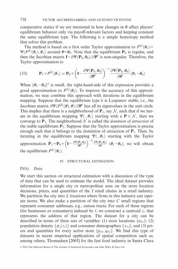
comparative statics if we are interested in how changes in h affect players�equilibrium behavior only via payoff-relevant factors and keeping constantthe same equilibrium type. The following is a simple homotopy methodthat solves this problem.

The method is based on a first order Taylor approximation to P½k�ðh1Þ5WðP½k�ðh1Þ; h1Þ around h5h0. Note that the equilibrium P0 is regular, andthen the Jacobian matrix I2@WðP0; h0Þ=@P0 is non-singular. Therefore, theTaylor approximation is:

P15P½k�ðh1Þ ’ P01 I2@WðP0; h0Þ

@P0

� 21 @WðP0; h0Þ@h0

ðh12h0Þ(33)

When kh12h0k2 is small, the right-hand-side of this expression provides agood approximation to P½k�ðh1Þ. To improve the accuracy of this approxi-mation, we may combine this approach with iterations in the equilibriummapping. Suppose that the equilibrium type k is Lyapunov stable, i.e., theJacobian matrix @WðP½k�ðhÞ; hÞ=@P0 has all its eigenvalues in the unit circle.This implies that there is a neighborhood of P1, say N , such that if we iter-ate in the equilibrium mapping Wð:; h1Þ starting with a P 2 N , then weconverge to P1. The neighborhood N is called the dominion of attraction ofthe stable equilibrium P1. Suppose that the Taylor approximation is preciseenough such that it belongs to the dominion of attraction of P1. Then, byiterating in the equilibrium mapping Wð:; h1Þ starting with the Taylor

approximation P15P01 I2 @WðP0;h0Þ@P0

�21@WðP0;h0Þ

@h0ðh12h0Þ, we will obtain

the equilibrium P½k�ðh1Þ.

IV. STRUCTURAL ESTIMATION

IV(i). Data

We start this section on structural estimation with a discussion of the typeof data that can be used to estimate the model. The ideal dataset providesinformation for a single city or metropolitan area on the store locationdecisions, prices, and quantities of the I retail chains in a retail industry.We partition the city into L locations where firms in this industry can oper-ate stores. We also make a partition of the city into C small regions thatrepresent consumer addresses, e.g., census tracts. For each of these regions(for businesses or consumers) indexed by ‘, we construct a centroid z‘ thatrepresents the address of that region. The dataset for a city can bedescribed in terms of three sets of variables: (1) store locations fni‘tg; (2)population density f/tðz‘Þg and consumer demographics fx‘tg; and (3) pri-ces and quantities for every active store fpi‘t; qi‘tg. We find this type ofdatasets in recent empirical applications of spatial competition such as,among others, Thomadsen [2005] for the fast food industry in Santa Clara



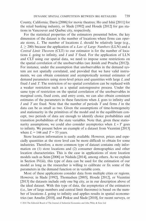
County, California; Davis [2006] for movie theatres; Ho and Ishii [2011] forthe retail banking industry, or Slade [1992] and Houde [2012] for gas sta-tions in Vancouver and Quebec city, respectively.

For the statistical properties of the estimators presented below, the keydimension of the dataset is the number of locations where firms can oper-ate stores, L. The number of locations L should be relatively large (e.g.,L � 200) because the application of a Law of Large Numbers (LLN) and aCentral Limit Theorem (CLT) to our estimator is for the number of loca-tions L going to infinity, and I and T fixed. For the application of LLNand CLT using our spatial data, we need to impose some restrictions onthe spatial correlation of the unobservables (see Jenish and Prucha [2012]).For instance, under the assumption that unobservables in the demand sys-tem are not spatially correlated, and provided that we have valid instru-ments, we can obtain consistent and asymptotically normal estimates ofdemand parameters using store-level prices and quantities with large L andfixed I and T. The restriction of no spatial correlation can be replaced witha weaker restriction such as a spatial autoregressive process. Under thesame type of restriction on the spatial correlation of the unobservables inmarginal costs, fixed costs, and entry costs, we can also obtain consistentestimates of the parameters in these functions when L goes to infinity andI and T are fixed. Note that the number of periods T and firms I in thedata can be as small as two. Given the assumptions of time-homogeneityand stationarity in the primitives of the model and in the equilibrium con-cept, two periods of data are enough to identify choice probabilities andtransition probabilities of the state variables. Note that, given these statio-narity assumptions, we could also consider asymptotics when L � T goesto infinity. We present below an example of a dataset from Vicentini [2013]where L 5 144 and T 5 55 years.

Store location information is easily available. However, prices and espe-cially quantities at the store level can be more difficult to obtain for someindustries. Therefore, a more common type of dataset contains only infor-mation on (1) store locations and (2) consumer demographics and otherlocation characteristics. This is the case in applications of store locationmodels such as Seim [2006] or Nishida [2014], among others. As we explainin Section IV(iii), this type of data can be used for the estimation of ourmodel as long as the researcher is willing to calibrate or fix some of theparameters in the demand function or in variable costs.

Most of these applications consider data from multiple cities or regions.However, in Slade [1992], Thomadsen [2005], Houde [2012], or Vicentini[2013] the datasets include only one big city, as in our description above ofthe ideal dataset. With this type of data, the asymptotics of the estimators(i.e., law of large numbers and central limit theorems) is based on the num-ber of locations L going to infinity and applies results in spatial econome-trics (see Anselin [2010], and Pinkse and Slade [2010], for recent surveys, or



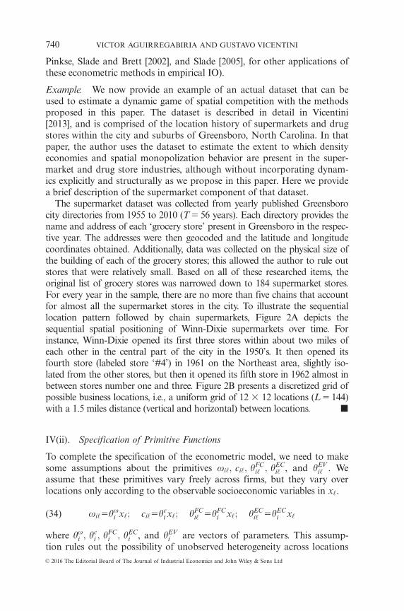
Pinkse, Slade and Brett [2002], and Slade [2005], for other applications ofthese econometric methods in empirical IO).

Example. We now provide an example of an actual dataset that can beused to estimate a dynamic game of spatial competition with the methodsproposed in this paper. The dataset is described in detail in Vicentini[2013], and is comprised of the location history of supermarkets and drugstores within the city and suburbs of Greensboro, North Carolina. In thatpaper, the author uses the dataset to estimate the extent to which densityeconomies and spatial monopolization behavior are present in the super-market and drug store industries, although without incorporating dynam-ics explicitly and structurally as we propose in this paper. Here we providea brief description of the supermarket component of that dataset.

The supermarket dataset was collected from yearly published Greensborocity directories from 1955 to 2010 (T 5 56 years). Each directory provides thename and address of each �grocery store� present in Greensboro in the respec-tive year. The addresses were then geocoded and the latitude and longitudecoordinates obtained. Additionally, data was collected on the physical size ofthe building of each of the grocery stores; this allowed the author to rule outstores that were relatively small. Based on all of these researched items, theoriginal list of grocery stores was narrowed down to 184 supermarket stores.For every year in the sample, there are no more than five chains that accountfor almost all the supermarket stores in the city. To illustrate the sequentiallocation pattern followed by chain supermarkets, Figure 2A depicts thesequential spatial positioning of Winn-Dixie supermarkets over time. Forinstance, Winn-Dixie opened its first three stores within about two miles ofeach other in the central part of the city in the 1950�s. It then opened itsfourth store (labeled store �#4�) in 1961 on the Northeast area, slightly iso-lated from the other stores, but then it opened its fifth store in 1962 almost inbetween stores number one and three. Figure 2B presents a discretized grid ofpossible business locations, i.e., a uniform grid of 12 3 12 locations (L 5 144)with a 1.5 miles distance (vertical and horizontal) between locations. �

IV(ii). Specification of Primitive Functions

To complete the specification of the econometric model, we need to makesome assumptions about the primitives xi‘; ci‘; hFC

i‘ ; hECi‘ , and hEV

i‘ . Weassume that these primitives vary freely across firms, but they vary overlocations only according to the observable socioeconomic variables in x‘.

xi‘5hxi x‘; ci‘5hc

i x‘; hFCi‘ 5hFC

i x‘; hECi‘ 5hEC

i x‘(34)

where hxi ; hc

i ; hFCi ; hEC

i , and hEVi are vectors of parameters. This assump-

tion rules out the possibility of unobserved heterogeneity across locations



Figure 2ASequential Location of Stores: Winn-Dixie

Notes: Solid gray line represents Greensboro 2000 urbanized area, and dotted gray line repre-sents Greensboro 1950 city limits, both based on U.S. Census boundary files.

Figure 2BConstruction of Business Locations: Greensboro, North Carolina

Notes: Solid gray line represents Greensboro 2000 urbanized area, and dotted gray line repre-sents Greensboro 1950 city limits, both based on U.S. Census boundary files.



‘, and therefore it may be a strong assumption in applications without arich set of observables in x‘.

24

Let x be the vector fx‘ : ‘51; 2; . . . ;Lg, that is a description of the�landscape� of observable socioeconomic characteristics in the city. All theanalysis is conditional on x. Given x, we can interpret the store networksin nt as a single realization of a spatial stochastic process. In terms of theeconometric analysis, this has similarities with time series econometrics inthe sense that a time series is a single realization from a stochastic process.Though we observe a single realization of this stochastic process, we canstill estimate consistently the parameters of that process as the number oflocations L goes to infinity.

IV(iii). Estimation

For estimation purposes, it is convenient to distinguish three subvectors inh. That is, h5fhD; hMC; hFCg where hD represents demand parameters fl,s, hx

i : i51; 2; . . . ; Ig; hMC contains parameters in marginal costsfhc

i : i51; 2; . . . ; Ig, and hFC contains parameters in fixed costs, entry costs,and exit values, fhFC

i ; hECi ; hEV

i : i51; 2; . . . ; Ig.The estimation of parameters in demand and marginal costs can follow

the well known approach in Berry, Levinsohn and Pakes [1996] and Nevo[2001] for the estimation of demand of differentiated products, i.e., the socalled BLP method. In fact, given the assumption of no unobserved loca-tion heterogeneity in xi‘, the estimation of hD can be much simpler than inthe BLP approach because there is no endogeneity of prices and no needto invert the relationship between market shares and average utilities.Therefore, a possible estimator of hD is a Nonlinear Least Squaresestimator:

hD5arg minhD

XI

i51

XL

‘51

si‘2X

k

ri‘ðz kð Þ; n; p; hDÞ/ z kð Þ� �" #2

(35)

where si‘ is the observed market share of store ði; ‘Þ (equals zero if thatstore does not exist), and ri‘ðz kð Þ; n; p; hDÞ is the multinomial logit probabil-ity that provides the proportion of consumers in location z kð Þ patronizingstore ði; ‘Þ. Given this estimation of demand, marginal costs parameters inhMC can be also estimated by least squares using the marginal conditionsof optimality for prices in equation (5). And given consistent estimators hD

and hMC , and the algorithm for computing the Bertrand equilibrium, wecan construct estimates of equilibrium variable profits, Ri ntð Þ, for anyobserved or hypothetical market structure nt.

24 This is a common assumption in some empirical applications, such as Seim [2006].



The restriction of no unobserved location heterogeneity in demand is astrong assumption. To relax this assumption, we need some instrumentsfor prices in the estimation of demand. For instance, suppose that someobservable exogenous variables in the vector x vary both across firms andover locations, i.e., xi‘. With this type of data, we could use the so-calledBLP instruments and method for the estimation of demand parameters.More specifically, we could obtain an equation that relates a known func-tion of store market shares with the average utility of purchasing in storeði; ‘Þ. In this equation, the observable characteristics of stores other thanði; ‘Þ, i.e., fxi‘ : j 6¼ ig, can be used to instrument for the price pi‘.

When data of prices and quantities at the store level is not available, theresearcher may be willing to calibrate the parameters of a parsimoniousspecification of demand and variable costs. Suppose that the researcher hasinformation on average price and aggregate quantity at the city-firm level,fPi;Qig. These 2 � I data points can be used to calibrate the parametersfl, s, x, cg under the assumption that firms have homogeneous qualitiesand unit costs. Another alternative is estimating jointly all the parametersof the model using the dynamic game and firms� store location decisions.

For the estimation of hFC, we exploit the restrictions imposed by theequilibrium of the dynamic game. Here we propose a two-step method forthe estimation of the dynamic game. Let P0 be the vector of CCP�s in theMPE in the city under study. We assume that there is a unique equilibriumin the data, i.e., the equilibrium does not vary over time or over regionswithin the city. We can use our approximation to firms� best response prob-ability functions WðSÞi ðaitjnt;P; hÞ evaluated at the true equilibrium P0 toconstruct the following likelihood function:

QðP; hÞ5Xi;t;‘

1fni‘t5ni‘t21gln WðSÞi ð0jnt;P; hÞ

1Xi;t;‘

1fni‘t2150; ni‘t51gln WðSÞi ð‘1jnt;P; hÞ

1Xi;t;‘

1fni‘t2151; ni‘t50gln WðSÞi ð‘2jnt;P; hÞ

(36)

Let P0 be a reduced-form nonparametric estimator of the populationCCP�s P0. We describe below how to obtain this estimator. Then, a consist-ent estimator of hFC can be obtained by maximizing the pseudo likelihoodfunction QðP0 ; hFC ; hD; hMCÞ with respect to hFC. The estimator is root-Lconsistent and asymptotically normal. This two-step method has been usedfor the estimation of dynamic games in IO applications in Ellickson, Bere-steanu and Misra [2010] or Sweeting [2013], among many others (seeAguirregabiria and Nevo [2013], for a survey of applications).



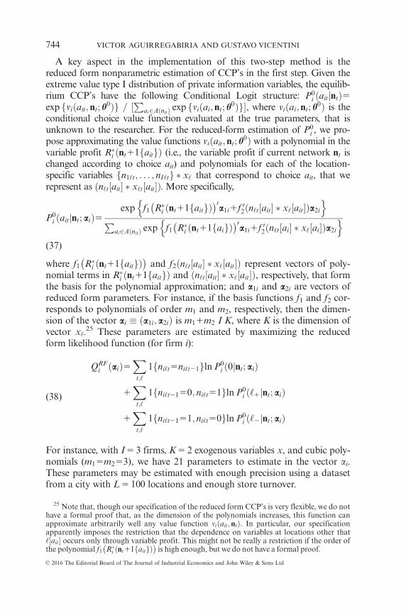
A key aspect in the implementation of this two-step method is thereduced form nonparametric estimation of CCP�s in the first step. Given theextreme value type I distribution of private information variables, the equilib-rium CCP�s have the following Conditional Logit structure: P0

i ðaitjntÞ5exp fviðait; nt; h

0Þg = ½P

ai2AðnitÞ exp fviðai; nt; h0Þg�, where viðai; nt; h

0Þ is theconditional choice value function evaluated at the true parameters, that isunknown to the researcher. For the reduced-form estimation of P0

i , we pro-pose approximating the value functions viðait; nt; h

0Þ with a polynomial in thevariable profit R�i ðnt11faitgÞ (i.e., the variable profit if current network nt ischanged according to choice ait) and polynomials for each of the location-specific variables fn1‘t; . . . ; nI‘tg � x‘ that correspond to choice ait, that werepresent as ðn‘t½ait� � x‘t½ait�Þ. More specifically,

P0i ðaitjnt; aiÞ5

exp f1 R�i ðnt11faitgÞ� �0

a1i1f 02ðn‘t½ait� � x‘½ait�Þa2i

n oP

ai2AðnitÞ exp f1 R�i ðnt11faigÞ� �0

a1i1f 02ðn‘t½ai� � x‘½ai�Þa2i

n o(37)

where f1 R�i ðnt11faitgÞ� �

and f2ðn‘t½ait� � x‘½ait�Þ represent vectors of poly-nomial terms in R�i ðnt11faitgÞ and ðn‘t½ait� � x‘½ait�Þ, respectively, that formthe basis for the polynomial approximation; and a1i and a2i are vectors ofreduced form parameters. For instance, if the basis functions f1 and f2 cor-responds to polynomials of order m1 and m2, respectively, then the dimen-sion of the vector ai � ða1i; a2iÞ is m11m2 I K, where K is the dimension ofvector x‘.

25 These parameters are estimated by maximizing the reducedform likelihood function (for firm i):

QRFi ðaiÞ5

Xt;‘

1fni‘t5ni‘t21gln P0i ð0jnt; aiÞ

1X

t;‘

1fni‘t2150; ni‘t51gln P0i ð‘1jnt; aiÞ

1X

t;‘

1fni‘t2151; ni‘t50gln P0i ð‘2jnt; aiÞ

(38)

For instance, with I 5 3 firms, K 5 2 exogenous variables x, and cubic poly-nomials (m15m253), we have 21 parameters to estimate in the vector ai.These parameters may be estimated with enough precision using a datasetfrom a city with L 5 100 locations and enough store turnover.

25 Note that, though our specification of the reduced form CCP�s is very flexible, we do nothave a formal proof that, as the dimension of the polynomials increases, this function canapproximate arbitrarily well any value function viðait; ntÞ. In particular, our specificationapparently imposes the restriction that the dependence on variables at locations other that‘½ait� occurs only through variable profit. This might not be really a restriction if the order ofthe polynomial f1 R�i ðnt11faitgÞ

� �is high enough, but we do not have a formal proof.



V. ENTRY COSTS AND THE DYNAMICS OF STORE LOCATION

We apply our model to analyze how changes in the cost of setting-up astore (entry costs) affect firms� strategies, firm value and consumer welfare.

V(i). Benchmark Model

The following parameters are constant over our experiments.

a. Market. The market is a square city of 10 3 10 kilometers:C5½0; 10�2. Consumers (households) are uniformly distributed on C

and the population size is equal to 100,000 households. Populationsize and the geographical distribution of consumers are constant overtime. There are 16 business locations (L 5 16) which form a uniformgrid in the square city. The coordinates of business locations are the16 points that result from the intersection of coordinates ð2; 4; 6; 8Þin the horizontal and vertical axes, i.e., z15 2; 2ð Þ; z25 2; 4ð Þ,. . .,z155 8; 6ð Þ; and z165 8; 8ð Þ. The unit transportation cost s, whichincludes the opportunity cost of travel time, is $5 per kilometer.26

b. Product and firms. Firms are supermarket chains. The product underconsideration is the weekly shopping basket of a family in a super-market. Therefore, xi represents the (average) willingness to pay forthe weekly shopping basket in supermarket chain i. There are twofirms in this city. These firms are identical in terms of the quality oftheir products. We fix x15x25$135. One period in the model is a cal-endar year and the discount factor is set at b50:9. Note that house-holds� willingness to pay (x5$135) and the transportation cost(s5$5=km) correspond to weekly shopping, while the frequency offirms� decisions is annual. Therefore, the correct definition of marketsize should be the number of households times the number of weeksper year: M 5 100, 000 3 5255; 200; 000 household-weeks. Theparameter l, that measures the degree of (non-spatial) horizontalproduct differentiation, is equal to $2.

c. Firms� costs. Firms are also identical in their cost structures. A firm�smarginal cost to provide the weekly shopping basket of a household is$100. Fixed operating costs and exit values are set to zero. The com-mon knowledge component of entry costs, hEC, is constant acrosslocations. We compute an equilibrium of the dynamic game under 21different values of hEC between $0 and $20 million. To give an idea ofthe relative magnitude of this range of entry costs, note that given thedemand and variable cost parameters that we have fixed, the totalvariable profit of a monopolist with one store at every location is

26 Suppose that most of the transportation cost comes from the opportunity cost of traveltime. If the average hourly wage is $30=hour and the average transportation speed in this cityis 6km=hour, then s5ð$30=hourÞ=ð6km=hourÞ5$5 per kilometer.



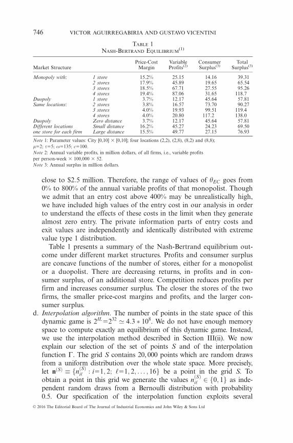
close to $2:5 million. Therefore, the range of values of hEC goes from0% to 800% of the annual variable profits of that monopolist. Thoughwe admit that an entry cost above 400% may be unrealistically high,we have included high values of the entry cost in our analysis in orderto understand the effects of these costs in the limit when they generatealmost zero entry. The private information parts of entry costs andexit values are independently and identically distributed with extremevalue type 1 distribution.

Table 1 presents a summary of the Nash-Bertrand equilibrium out-come under different market structures. Profits and consumer surplusare concave functions of the number of stores, either for a monopolistor a duopolist. There are decreasing returns, in profits and in con-sumer surplus, of an additional store. Competition reduces profits perfirm and increases consumer surplus. The closer the stores of the twofirms, the smaller price-cost margins and profits, and the larger con-sumer surplus.

d. Interpolation algorithm. The number of points in the state space of thisdynamic game is 2IL5232 ’ 4:3 � 108. We do not have enough memoryspace to compute exactly an equilibrium of this dynamic game. Instead,we use the interpolation method described in Section III(ii). We nowexplain our selection of the set of points S and of the interpolationfunction C. The grid S contains 20, 000 points which are random drawsfrom a uniform distribution over the whole state space. More precisely,let nðSÞ � fnðSÞi‘ : i51; 2; ‘51; 2; . . . ; 16g be a point in the grid S. Toobtain a point in this grid we generate the values nðSÞi‘ 2 f0; 1g as inde-pendent random draws from a Bernoulli distribution with probability0.5. Our specification of the interpolation function exploits several

TABLE 1NASH-BERTRAND EQUILIBRIUM

(1)

Market StructurePrice-Cost

MarginVariableProfits(2)

ConsumerSurplus(3)

TotalSurplus(3)

Monopoly with: 1 store 15.2% 25.15 14.16 39.312 stores 17.9% 45.89 19.65 65.543 stores 18.5% 67.71 27.55 95.264 stores 19.4% 87.06 31.65 118.7

Duopoly 1 store 3.7% 12.17 45.64 57.81Same locations: 2 stores 3.8% 16.57 73.70 90.27

3 stores 4.0% 19.93 99.51 119.44 stores 4.0% 20.80 117.2 138.0

Duopoly Zero distance 3.7% 12.17 45.64 57.81Different locations Small distance 16.2% 45.27 24.23 69.50one store for each firm Large distance 15.5% 49.77 27.15 76.93

Note 1: Parameter values: City [0,10] 3 [0,10]; four locations (2,2), (2,8), (8,2) and (8,8);l52; s55; x5135; c5100:Note 2: Annual variable profits, in million dollars, of all firms, i.e., variable profitsper person-week 3 100,000 3 52:Note 3: Annual surplus in million dollars.



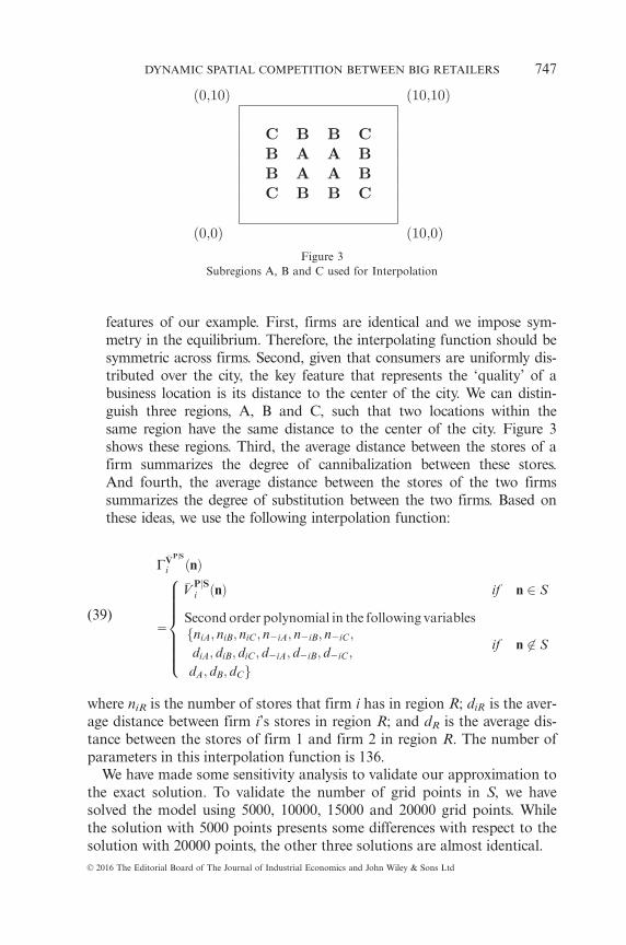
features of our example. First, firms are identical and we impose sym-metry in the equilibrium. Therefore, the interpolating function should besymmetric across firms. Second, given that consumers are uniformly dis-tributed over the city, the key feature that represents the �quality� of abusiness location is its distance to the center of the city. We can distin-guish three regions, A, B and C, such that two locations within thesame region have the same distance to the center of the city. Figure 3shows these regions. Third, the average distance between the stores of afirm summarizes the degree of cannibalization between these stores.And fourth, the average distance between the stores of the two firmssummarizes the degree of substitution between the two firms. Based onthese ideas, we use the following interpolation function:

C�VPjS

i ðnÞ

5

�V PjSi ðnÞ if n 2 S

Second order polynomial in the following variablesfniA; niB; niC ; n2iA; n2iB; n2iC ;

diA; diB; diC ; d2iA; d2iB; d2iC ;

dA; dB; dCg

if n 62 S

8>>>>>><>>>>>>:

(39)

where niR is the number of stores that firm i has in region R; diR is the aver-age distance between firm i�s stores in region R; and dR is the average dis-tance between the stores of firm 1 and firm 2 in region R. The number ofparameters in this interpolation function is 136.

We have made some sensitivity analysis to validate our approximation tothe exact solution. To validate the number of grid points in S, we havesolved the model using 5000, 10000, 15000 and 20000 grid points. Whilethe solution with 5000 points presents some differences with respect to thesolution with 20000 points, the other three solutions are almost identical.

Figure 3Subregions A, B and C used for Interpolation



To validate the interpolation function (39) we have applied this functionto similar but much smaller problems for which we can compare theapproximation to the exact solution of the game. We have considered thesame dynamic game but with four locations instead of 16. The market isstill the square city of 10 3 10 kilometers, C5½0; 10�2, but there are onlyfour business locations which are located in a straight line along the city�smain street with coordinates z15ð2; 5Þ; z25ð4; 5Þ; z35ð6; 5Þ, and z45ð8; 5Þ.For this simpler game the state space has 21051024 cells. For the interpola-tion function we consider only two regions (A and B) according to the dis-tance to the city center, such that locations z25ð4; 5Þ and z35ð6; 5Þ are inregion A (with distance to the center equal to 1), and locations z15ð2; 5Þand z45ð8; 5Þ are in region B (with distance to the center equal to 3). Theinterpolation function is a second order polynomial in the variablesfniA,niB, n2iA; n2iB,di, d2ig and it has 28 parameters. The experiment showsthat this interpolation function provides an excellent approximation to thetrue value function and to the equilibrium choice probabilities in this exam-ple. More generally, we conjecture that for specifications where firms aresymmetric, consumers are uniformly distributed and business locationshave a symmetric spatial structure, this type of interpolation function mayprovide a good approximation to the exact solution of the game.

V(ii). Results

Figures 4 to 8 summarize the results of our numerical experiments. Each ofthese figures presents an outcome variable of the game (e.g., average num-ber of stores) in the vertical axis as a function of the entry cost parameterhEC in the horizontal axis. To analyze the effects of competition we repre-sent these functions both for a duopoly model and for a monopolist with-out threat of potential entrants. In the horizontal axis, the entry cost ismeasured as a percentage of the annual variable profit of a monopolist withstores at every business location. Some of the outcome variables (e.g., num-ber of stores, consumer welfare, value of a firm, average distance betweenstores) are calculated using the steady-state distribution of state variableswhich is implied by the Markov perfect equilibrium. We have used thehomotopy method described in Section III(iii) to guarantee that we selectthe same type of equilibrium when we vary the value of the entry cost.

a. Figure 4: Store turnover: openings and shutdowns.27 Figure 4 presentsthe average number of store openings per year and firm. As onewould expect, an increase in the entry cost always reduces store open-ings and shutdowns. For most values of the entry cost, store turnoveris similar under monopoly and duopoly. Nevertheless, for entry costs

27 In steady-state the number of store openings should be equal to the number of storeshutdowns.



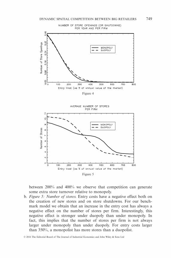
between 200% and 400% we observe that competition can generatesome extra store turnover relative to monopoly.

b. Figure 5: Number of stores. Entry costs have a negative effect both onthe creation of new stores and on store shutdowns. For our bench-mark model we obtain that an increase in the entry cost has always anegative effect on the number of stores per firm. Interestingly, thisnegative effect is stronger under duopoly than under monopoly. Infact, this implies that the number of stores per firm is not alwayslarger under monopoly than under duopoly. For entry costs largerthan 350%, a monopolist has more stores than a duopolist.

Figure 4

Figure 5



c. Figures 6, 7 and 8: Consumer welfare and value of a firm. Given thenegative effect of entry costs on the number of stores, consumer wel-fare also declines with entry costs. Furthermore, despite entry costs�having a stronger effect on the number of stores under duopoly, con-sumer welfare is always around 50% larger under duopoly than undermonopoly. This is because the monopolist offsets a reduction in con-sumer transportation costs with higher prices. The value of a firm, inFigure 7, and total welfare, in Figure 8, decline monotonically withentry costs. Welfare is always greater under duopoly.

Figure 6

Figure 7



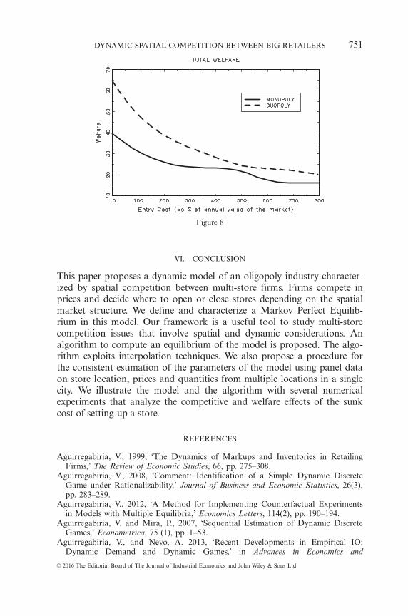
VI. CONCLUSION

This paper proposes a dynamic model of an oligopoly industry character-ized by spatial competition between multi-store firms. Firms compete inprices and decide where to open or close stores depending on the spatialmarket structure. We define and characterize a Markov Perfect Equilib-rium in this model. Our framework is a useful tool to study multi-storecompetition issues that involve spatial and dynamic considerations. Analgorithm to compute an equilibrium of the model is proposed. The algo-rithm exploits interpolation techniques. We also propose a procedure forthe consistent estimation of the parameters of the model using panel dataon store location, prices and quantities from multiple locations in a singlecity. We illustrate the model and the algorithm with several numericalexperiments that analyze the competitive and welfare effects of the sunkcost of setting-up a store.

REFERENCES

Aguirregabiria, V., 1999, �The Dynamics of Markups and Inventories in RetailingFirms,� The Review of Economic Studies, 66, pp. 275–308.

Aguirregabiria, V., 2008, �Comment: Identification of a Simple Dynamic DiscreteGame under Rationalizability,� Journal of Business and Economic Statistics, 26(3),pp. 283–289.

Aguirregabiria, V., 2012, �A Method for Implementing Counterfactual Experimentsin Models with Multiple Equilibria,� Economics Letters, 114(2), pp. 190–194.

Aguirregabiria, V. and Mira, P., 2007, �Sequential Estimation of Dynamic DiscreteGames,� Econometrica, 75 (1), pp. 1–53.

Aguirregabiria, V., and Nevo, A. 2013, �Recent Developments in Empirical IO:Dynamic Demand and Dynamic Games,� in Advances in Economics and

Figure 8



Econometrics. Tenth World Congress. Volume 3, Econometrics. Acemoglu, D.; Are-llano, M. and Deckel, E. (eds).

Aguirregabiria, V. and Vicentini, G., 2012, �Software for the Computation of MarkovPerfect Equilibria in a Dynamic Model of Spatial Competition,� manuscript(Department of Economics. University of Toronto, Toronto, Canada).

Anderson, S.; De Palma, A. and Thisse, J.-F., 1992, �Discrete Choice Theory of Prod-uct Differentiation,� (MIT Press, Cambridge, Massachusetts, U.S.A).

Anselin, L., 2010, �Thirty Years of Spatial Econometrics,� Papers in Regional Science,89(1), pp. 3–25.

Bajari, P.; Benkard, L. and Levin, J., 2007, �Estimating Dynamic Models of Imper-fect Competition,� Econometrica, 75(5), pp. 1331–1370.

Baker, J., 1997, �Product Differentiation Through Time and Space: Antitrust PolicyIssues,� FTC Antitrust Bulletin, 42, pp. 177–196.

Bernstein, F. and K€ok, G., 2009, �Dynamic Cost Reduction through ProcessImprovement in Assembly Networks,� Management Science, 55(4), pp. 552–67.

Berry, S., 1994, �Estimating Discrete Choice Models of Product Differentiation,�RAND Journal of Economics, 25(2), pp. 242–262.

Berry, S.; Levinsohn, J. and Pakes, A., 1996, �Automobile Prices in Market Equi-librium,� Econometrica, 63(4), pp. 841–890.

Bertsekas, D. and Tsitsiklis, J., 1996, �Neuro-Dynamic Programming,� (Athena Scien-tific, Belmont, Massachusetts, U.S.A).

Bonanno, G., 1987, �Location Choice, Product Proliferation and Entry Deterrance,�Review of Economic Studies, 54, pp. 37–45.

Curtat, L., 1996, �Markov Equilibria of Stochastic Games with Complementarities,�Games and Economic Behavior, 17, pp. 177–199.

Datta, S. and Sudhir, K., 2011, �The Agglomeration-Differentiation Tradeoff in SpatialLocation Choice,� manuscript (Yale School of Management, Yale University, NewHaven, Connecticut, U.S.A).

Davis, P., 2006, �Spatial Competition in Retail Markets: Movie Theaters,� the RANDJournal of Economics, 37(4), pp. 964–982.

De Palma, A.; Ginsburgh, V.; Papageorgiou, Y. and Thisse, J.-F., 1985, �The Principleof Minimum Differentiation Holds Under Sufficient Heterogeneity,� Econometrica,53(4), pp. 767–781.

Doraszelski, U. and Escobar, J., 2010, �A Theory of Regular Markov Perfect Equili-bria in Dynamic Stochastic Games: Genericity, Stability and Purification,� Theo-retical Economics, 5, pp. 369–402.

Doraszelski, U. and Satterthwaite, M., 2010, �Computable Markov-Perfect IndustryDynamics,� RAND Journal of Economics, 41(2), pp. 215–243.

Eaton, C. and Lipsey, R., 1975, �The Principle of Minimum Differentiation Recon-sidered: Some New Developments in the Theory of Spatial Competition,� Reviewof Economic Studies, 42(1), pp. 27–50.

Echenique, F., 2007, �Finding All Equilibria in Games of Strategic Complements,�Journal of Economic Theory, 135(1), pp. 514–532.

Eckert, A. and West, D., 2008, �Radius Restrictions and the Similarity of NeighboringShopping Centers,� International Journal of the Economics of Business, 15, pp. 281–300.

Ellickson, P.; Beresteanu A. and Misra, S., 2010, �The Dynamics of Retail Oligopoly,�working paper (Duke University, Durham, North Carolina, U.S.A).

Ellickson, P.; Houghton S. and Timmins, C., 2013, �Estimating Network Economiesin Retail Chains: A Revealed Preference Approach,� RAND Journal of Economics,44(2), pp. 169–193.

Ericson, R. and Pakes, A., 1995, �Markov-Perfect Industry Dynamics: A Frameworkfor Empirical Work,� Review of Economic Studies, 62, pp. 53–82.



Hay, D. A., 1976, �Sequential Entry and Entry-Deterring Strategies in Spatial Com-petition,� Oxford Economic Papers, 28(2), pp. 240–257.

Ho, K., and Ishii, J., 2011, �Location and Competition in Retail Banking,� Interna-tional Journal of Industrial Organization, 29(5), pp. 537–546.

Hollander, S. and Omura, G., 1989, �Chain Store Developments and Their Political,Strategic and Social Interdependencies,� Journal of Retailing, 65(3), pp. 299–325.

Holmes, T., 2011, �The Diffusion of Wal-Mart and Economies of Density,� Econo-metrica, 79(1), pp. 253–302.

Hotelling, H., 1929, �Stability in Competition,� Economic Journal, 39, pp. 41–57.Jarmin, R., Klimek, S. and Miranda, J. 2009, �The Role of Retail Chains: National,

Regional and Industry Results,� in Producer Dynamics: New Evidence from MicroData, Dunne, T., Jensen, J. B. and Roberts M. J. (edis). NBER Book Series Stud-ies in Income and Wealth, (University of Chicago Press, Chicago, Illinois, U.S.A.).

Houde, Jean-Francois, 2012, �Spatial Differentiation and Vertical Mergers in RetailMarkets for Gasoline,� American Economic Review, 102(5), pp. 2147–2182.

Jenish, N. and Prucha, I., 2012, �On Spatial Processes and Asymptotic Inferenceunder Near-Epoch Dependence,� Journal of Econometrics, 170(1), pp. 178–190.

Jia, P., 2008, �What Happens when Wal-Mart Comes to Town: An Empirical Analy-sis of the Discount Retailing Industry,� Econometrica, 76(6), pp. 1263–1316.

Judd, K., 1985, �Credible Spatial Preemption,� RAND Journal of Economics, 16, pp.153–166.

Judd, K., 1998, Numerical Methods in Economics, (The MIT Press. Cambridge, Mas-sachusetts, U.S.A).

Larson, R. and Casti., J., 1982, Principles of Dynamic Programming, Part II. (Dek-ker, New York, New York, U.S.A).

Nevo, A., 2001, �Measuring Market Power in the Ready-to-Eat Cereal Industry,�Econometrica, 69(2), 307–342.

Nishida, M., 2015, �Esmating a Model of Strategic Network Choice: TheConvenience-Store Industry in Okinawa,� Marketing Science, 34, pp. 20–38.

Pakes, A. and McGuire, P., 1994, �Computing Markov-Perfect Nash Equilibria:Numerical Implications of a Dynamic Differentiated Product Model,� RAND Jour-nal of Economics, 25(4), pp. 555–589.

Pakes, A.; Ostrovsky, M. and Berry, S., 2007, �Simple Estimators for the Parametersof Discrete Dynamic Games, with Entry/Exit Examples,� RAND Journal of Eco-nomics, 38(2), pp. 373–399.

Pinkse, J. and Slade, M. E., 2010, �The Future Of Spatial Econometrics,� Journal ofRegional Science, 50(1), pp. 103–117.

Pinkse, J., Slade, M. E. and Brett, C., 2002, �Spatial Price Competition: A Semipara-metric Approach,� Econometrica, 70(3), pp. 1111–1153.

Rust, J., 1987, �Optimal Replacement of GMC Bus Engines: An Empirical Model ofHarold Zurcher,� Econometrica, 55(5), pp. 999–1033.

Rust, J., 1996, �Numerical Dynamic Programming in Economics,� in Amman, H.;Kendrick, D. and Rust, J. (eds.) Handbook of Computational Economics, Vol. 1.,(North-Holland Press, Amsterdam, The Netherlands).

Rust, J., 1997, �Using Randomization to Break the Curse of Dimensionality,� Econo-metrica, 65, pp. 487–516.

Ryan, S., 2012, �The Costs of Environmental Regulation in a Concentrated Industry,�Econometrica, 80(3), pp. 1019–1061.

Schmalensee, R., 1978, �Entry Deterrance in the Ready-to-Eat Breakfast CerealIndustry,� Bell Journal of Economics, 9, pp. 305–327.

Seim, K., 2006, �An Empirical Model of Firm Entry with Endogenous Product-typeChoices,� RAND Journal of Economics, 37(3), pp. 619–640.



Slade, M., 1992, �Vancouver�s Gasoline-Price Wars: An Empirical Exercise in Uncov-ering Supergame Strategies,� The Review of Economic Studies, 59(2), pp. 257–276.

Slade, M., 2005, �The Role of Economic Space in Decision Making,� Annalesd�Economie et de Statistique, 77, pp. 1–20.

Sweeting, A., 2013, �Dynamic Product Positioning in Differentiated Product Mar-kets: The Effect of Fees for Musical Performance Rights on the CommercialRadio Industry,� Econometrica, 81(5), pp. 1763–1803.

Tabuchi, T., 1994, �Two-Stage Two-Dimensional Spatial Competition between TWOFIRMS,� Regional Science and Urban Economics, 24(2), pp. 207–227.

Thomadsen, R., 2005, �The Effect of Ownership Structure on Prices in Geographi-cally Differentiated Industries,� The RAND Journal of Economics, 36(4), pp. 908–929.

Topkis, D., 1979, �Equilibrium Points in Nonzero-Sum N-person SubmodularGames,� SIAM Journal of Control and Optimization, 17(6), pp. 773–787.

Topkis, D., 1998, Supermodularity and Complementarity (Princeton University Press,Princeton, New Jersey, U.S.A).

Vicentini, G., 2013, �Location Strategy of Chain Retailers: The Case of Supermarketsand Drug Stores in an Urban Market,� manuscript (Northeastern University, Bos-ton, Massachusetts, U.S.A).

Vitorino, M. A., 2012, �Empirical Entry Games with Complementarities: An Appli-cation to the Shopping Center Industry,� Journal of Marketing Research, 49, pp.175–191.

Vives, X., 1999, Oligopoly Pricing (The MIT Press. Cambridge, Massachusetts,U.S.A).

West, D., 1981a, �Testing for Market Preemption Using Sequential Location Data,�Bell Journal of Economics, 12(1), pp. 129–143.

West, D., 1981b, �Tests of Two Locational Implications of a Theory of Market Pre-Emption,� Canadian Journal of Economics, 14(2), pp. 313–326.

Willig, R., 1991, �Merger Analysis, Industrial Organization Theory and MergerGuidelines,� Brookings Papers on Economic Activity - Microeconomics, 1991, pp.281–332.

Zhu, T. and Singh, V., 2009, �Spatial Competition with Endogenous LocationChoices: An Application to Discount Retailing,� Quantitative Marketing and Eco-nomics, 7(1), pp. 1–35.



Dynamic Spatial Competition Between Multi‐Store...

Documents

Transcript of Dynamic Spatial Competition Between Multi‐Store...