Technical WorkGroup

Meeting

Q3 2013 TWG

Geomorphology

Studies

September 25, 2013

Prepared by

Tetra Tech. Inc.

Watershed GeoDynamics

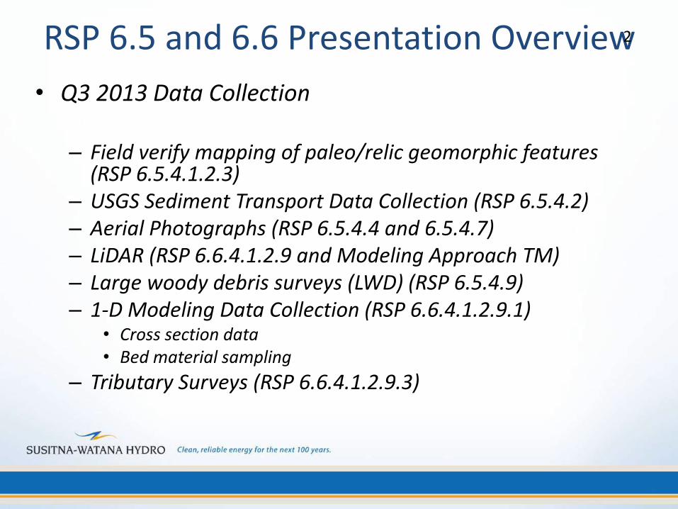
RSP 6.5 and 6.6 Presentation Overview 2

• Q3 2013 Data Collection – Field verify mapping of paleo/relic geomorphic features

(RSP 6.5.4.1.2.3) – USGS Sediment Transport Data Collection (RSP 6.5.4.2) – Aerial Photographs (RSP 6.5.4.4 and 6.5.4.7) – LiDAR (RSP 6.6.4.1.2.9 and Modeling Approach TM) – Large woody debris surveys (LWD) (RSP 6.5.4.9) – 1-D Modeling Data Collection (RSP 6.6.4.1.2.9.1)

• Cross section data • Bed material sampling

– Tributary Surveys (RSP 6.6.4.1.2.9.3)

Presentation Overview (Cont.) 3

– 2-D Modeling / Focus Area (RSP6.6.4.1.2.9.2)

• Bathymetry and topography

• Bed material sampling

• Geomorphic mapping and assessment

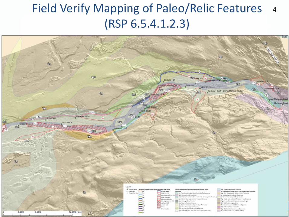
Field Verify Mapping of Paleo/Relic Features (RSP 6.5.4.1.2.3)

4

USGS Sediment Transport Data Collection 1980s and Current (RSP 6.5.4.2)

5

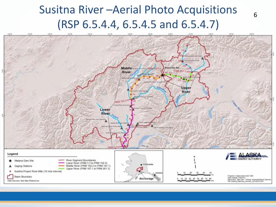
Susitna River –Aerial Photo Acquisitions (RSP 6.5.4.4, 6.5.4.5 and 6.5.4.7)

6

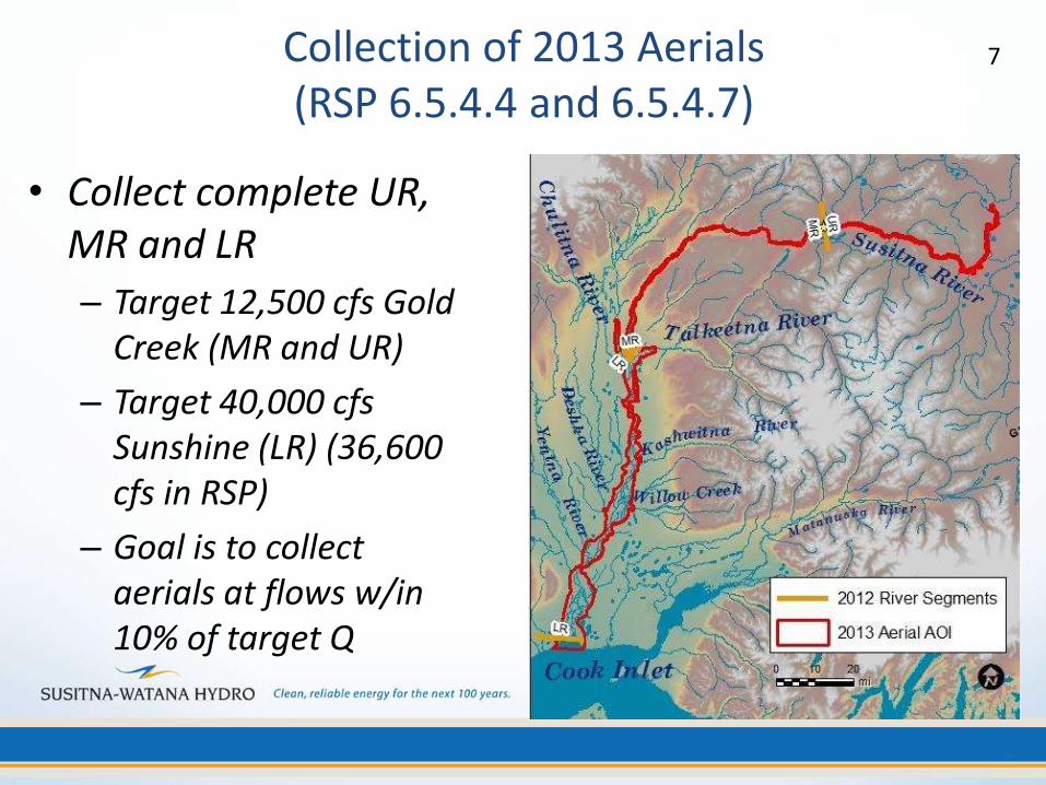
Collection of 2013 Aerials (RSP 6.5.4.4 and 6.5.4.7)

• Collect complete UR, MR and LR

– Target 12,500 cfs Gold Creek (MR and UR)

– Target 40,000 cfs Sunshine (LR) (36,600 cfs in RSP)

– Goal is to collect aerials at flows w/in 10% of target Q

7

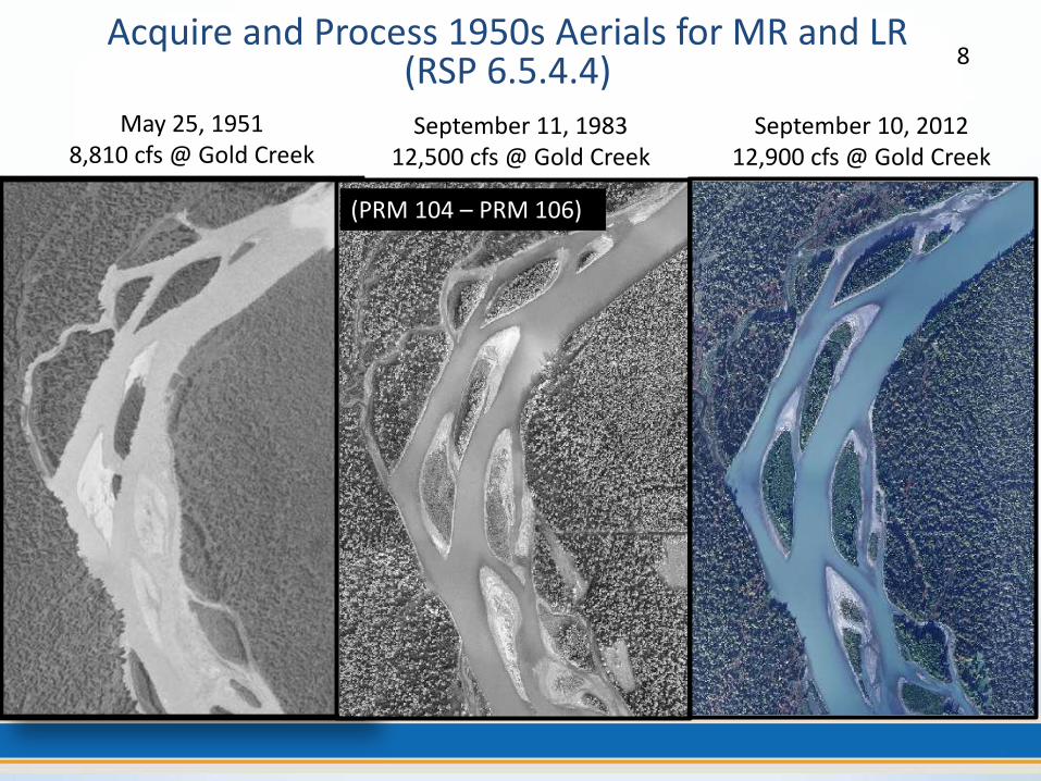
Acquire and Process 1950s Aerials for MR and LR (RSP 6.5.4.4) 8

September 10, 2012 12,900 cfs @ Gold Creek

September 11, 1983 12,500 cfs @ Gold Creek

May 25, 1951 8,810 cfs @ Gold Creek

(PRM 104 – PRM 106)

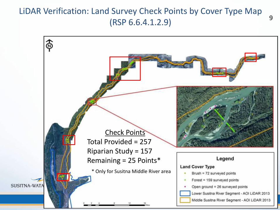
LiDAR Verification: Land Survey Check Points by Cover Type Map (RSP 6.6.4.1.2.9)

* Only for Susitna Middle River area

Check Points Total Provided = 257 Riparian Study = 157 Remaining = 25 Points*

9

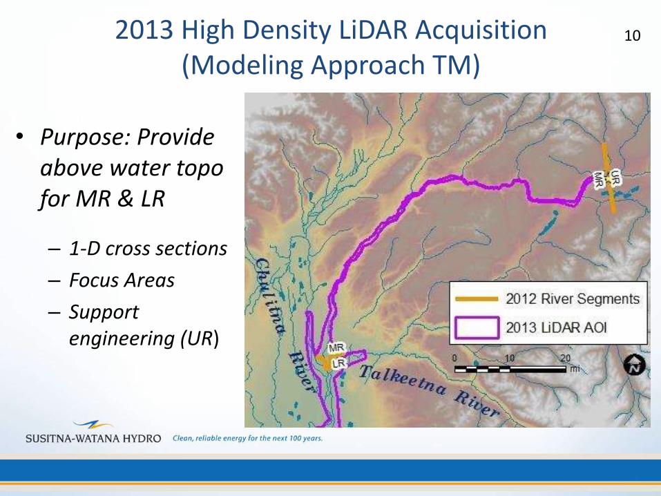
2013 High Density LiDAR Acquisition (Modeling Approach TM)

• Purpose: Provide above water topo for MR & LR

– 1-D cross sections

– Focus Areas

– Support engineering (UR)

10

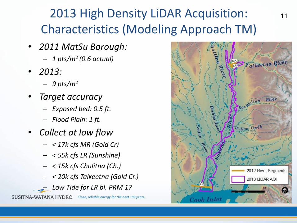
2013 High Density LiDAR Acquisition: Characteristics (Modeling Approach TM)

• 2011 MatSu Borough: – 1 pts/m2 (0.6 actual)

• 2013: – 9 pts/m2

• Target accuracy – Exposed bed: 0.5 ft.

– Flood Plain: 1 ft.

• Collect at low flow – < 17k cfs MR (Gold Cr)

– < 55k cfs LR (Sunshine)

– < 15k cfs Chulitna (Ch.)

– < 20k cfs Talkeetna (Gold Cr.)

– Low Tide for LR bl. PRM 17

11

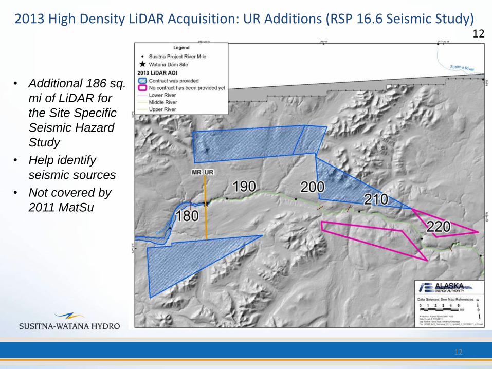
• Additional 186 sq.

mi of LiDAR for

the Site Specific

Seismic Hazard

Study

• Help identify

seismic sources

• Not covered by

2011 MatSu

12

12 2013 High Density LiDAR Acquisition: UR Additions (RSP 16.6 Seismic Study)

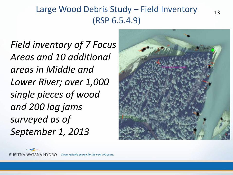
Large Wood Debris Study – Field Inventory (RSP 6.5.4.9)

13

Field inventory of 7 Focus Areas and 10 additional areas in Middle and Lower River; over 1,000 single pieces of wood and 200 log jams surveyed as of September 1, 2013

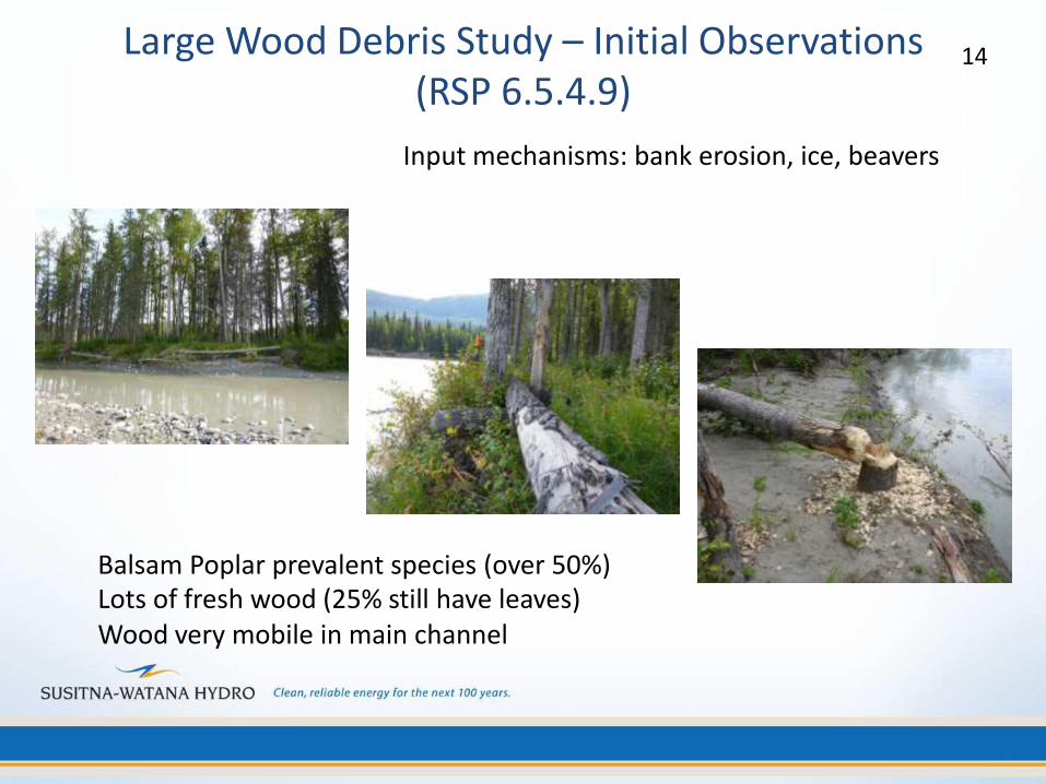
Large Wood Debris Study – Initial Observations (RSP 6.5.4.9)

14

Balsam Poplar prevalent species (over 50%) Lots of fresh wood (25% still have leaves) Wood very mobile in main channel

Input mechanisms: bank erosion, ice, beavers

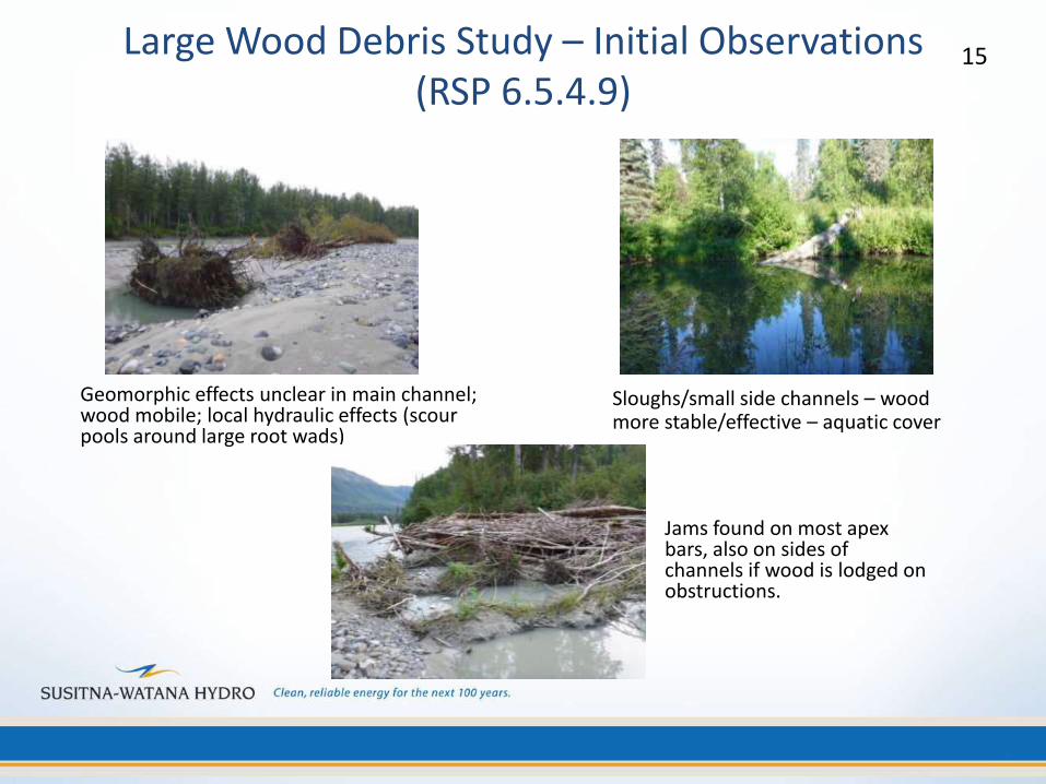
Large Wood Debris Study – Initial Observations (RSP 6.5.4.9)

15

Geomorphic effects unclear in main channel; wood mobile; local hydraulic effects (scour pools around large root wads)

Jams found on most apex bars, also on sides of channels if wood is lodged on obstructions.

Sloughs/small side channels – wood more stable/effective – aquatic cover

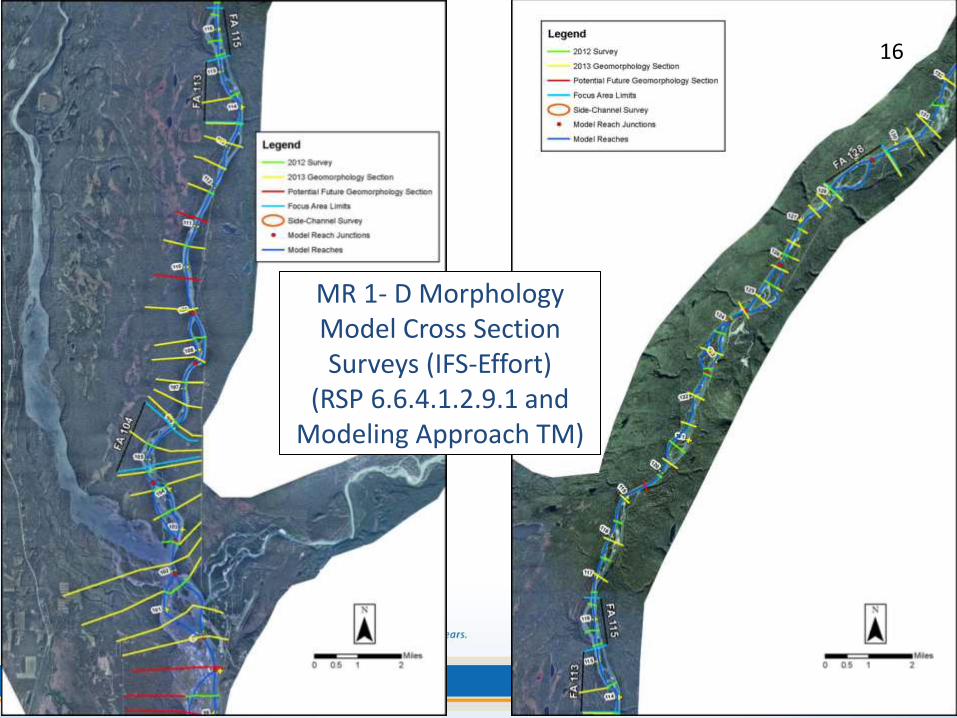
MR 1- D Morphology Model Cross Section Surveys (IFS-Effort)

(RSP 6.6.4.1.2.9.1 and Modeling Approach TM)

16

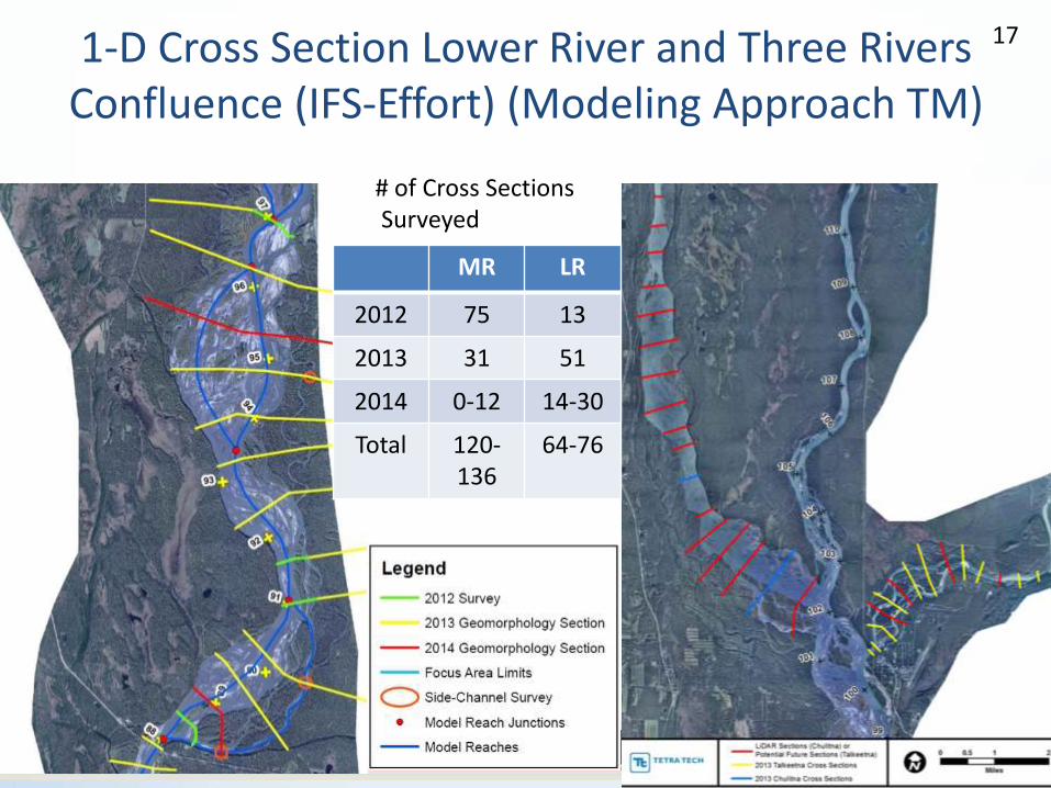
1-D Cross Section Lower River and Three Rivers Confluence (IFS-Effort) (Modeling Approach TM)

MR LR

2012 75 13

2013 31 51

2014 0-12 14-30

Total 120-136

64-76

# of Cross Sections Surveyed

17

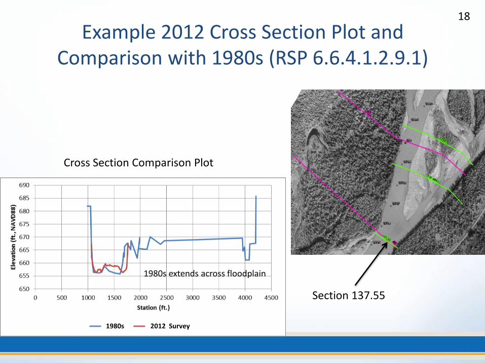
Example 2012 Cross Section Plot and Comparison with 1980s (RSP 6.6.4.1.2.9.1)

2012 Survey 1980s

1980s extends across floodplain

Section 137.55

Cross Section Comparison Plot

18

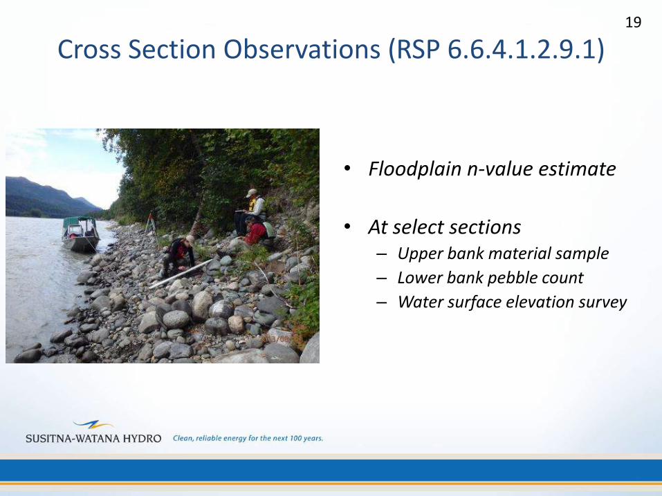
Cross Section Observations (RSP 6.6.4.1.2.9.1)

• Floodplain n-value estimate

• At select sections – Upper bank material sample

– Lower bank pebble count

– Water surface elevation survey

19

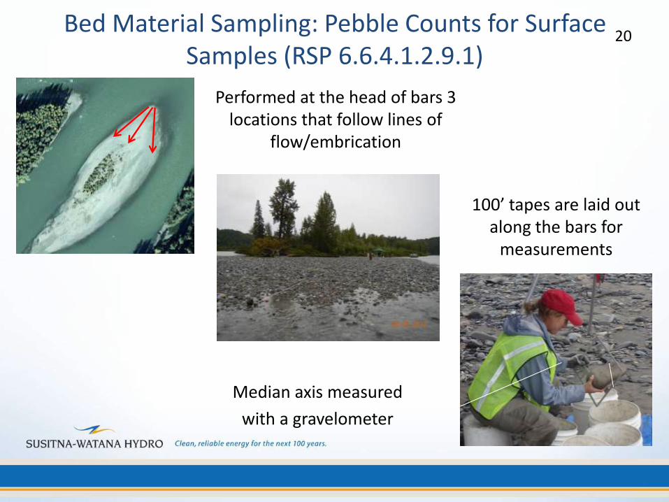
Bed Material Sampling: Pebble Counts for Surface Samples (RSP 6.6.4.1.2.9.1)

20

Performed at the head of bars 3 locations that follow lines of

flow/embrication

Median axis measured

with a gravelometer

100’ tapes are laid out along the bars for

measurements

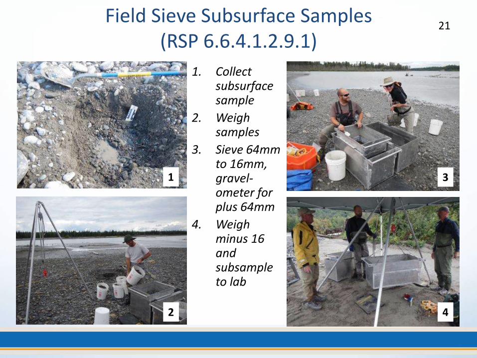
21 Field Sieve Subsurface Samples

(RSP 6.6.4.1.2.9.1)

1. Collect subsurface sample

2. Weigh samples

3. Sieve 64mm to 16mm, gravel-ometer for plus 64mm

4. Weigh minus 16 and subsample to lab

1

2

3

4

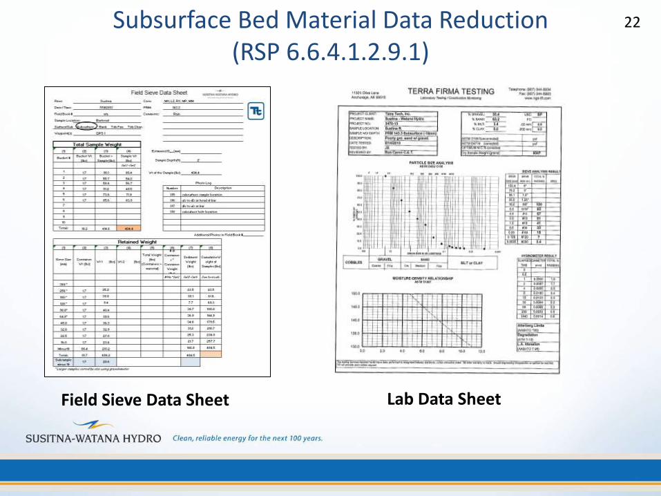
Subsurface Bed Material Data Reduction (RSP 6.6.4.1.2.9.1)

Field Sieve Data Sheet Lab Data Sheet

22

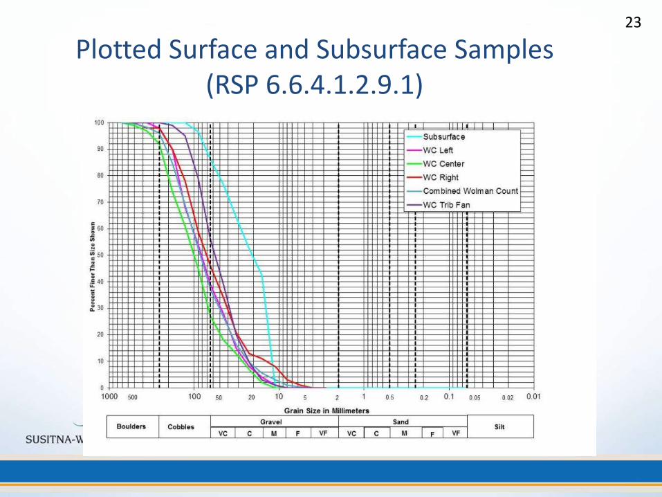
Plotted Surface and Subsurface Samples (RSP 6.6.4.1.2.9.1)

23

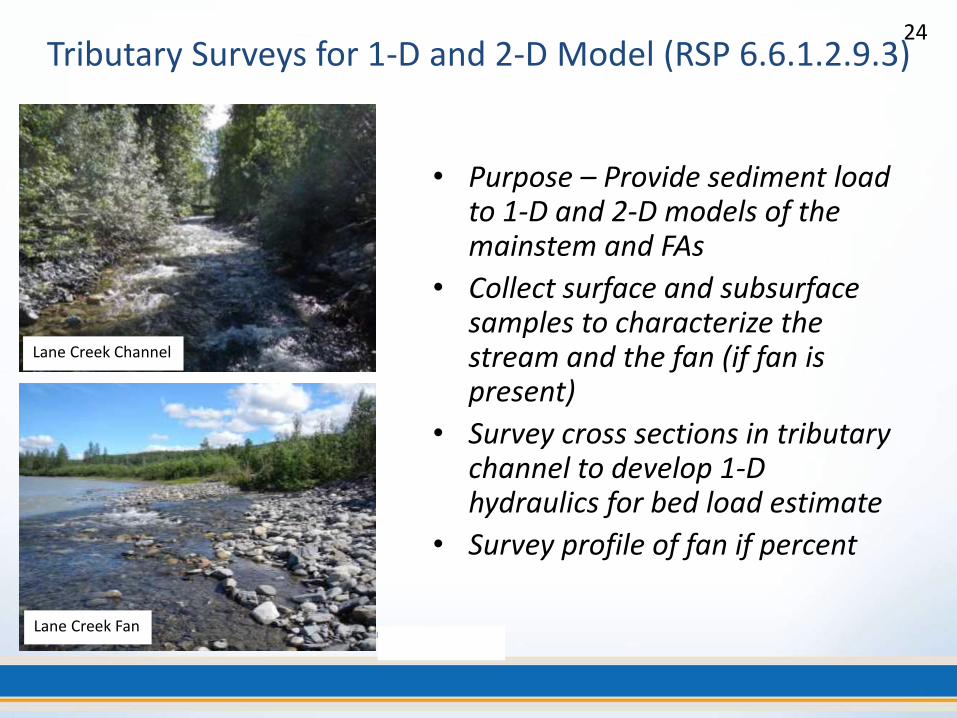
Tributary Surveys for 1-D and 2-D Model (RSP 6.6.1.2.9.3) 24

Lane Creek Channel

• Purpose – Provide sediment load to 1-D and 2-D models of the mainstem and FAs

• Collect surface and subsurface samples to characterize the stream and the fan (if fan is present)

• Survey cross sections in tributary channel to develop 1-D hydraulics for bed load estimate

• Survey profile of fan if percent

Lane Creek Fan

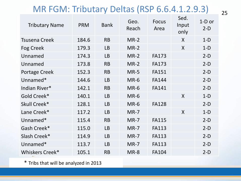
MR FGM: Tributary Deltas (RSP 6.6.4.1.2.9.3)

Tributary Name PRM Bank Geo.

Reach

Focus Area

Sed. Input only

1-D or 2-D

Tsusena Creek 184.6 RB MR-2 X 1-D

Fog Creek 179.3 LB MR-2 X 1-D

Unnamed 174.3 LB MR-2 FA173 2-D

Unnamed 173.8 RB MR-2 FA173 2-D

Portage Creek 152.3 RB MR-5 FA151 2-D

Unnamed* 144.6 LB MR-6 FA144 2-D

Indian River* 142.1 RB MR-6 FA141 2-D

Gold Creek* 140.1 LB MR-6 X 1-D

Skull Creek* 128.1 LB MR-6 FA128 2-D

Lane Creek* 117.2 LB MR-7 X 1-D

Unnamed* 115.4 RB MR-7 FA115 2-D

Gash Creek* 115.0 LB MR-7 FA113 2-D

Slash Creek* 114.9 LB MR-7 FA113 2-D

Unnamed* 113.7 LB MR-7 FA113 2-D

Whiskers Creek* 105.1 RB MR-8 FA104 2-D

25

* Tribs that will be analyzed in 2013

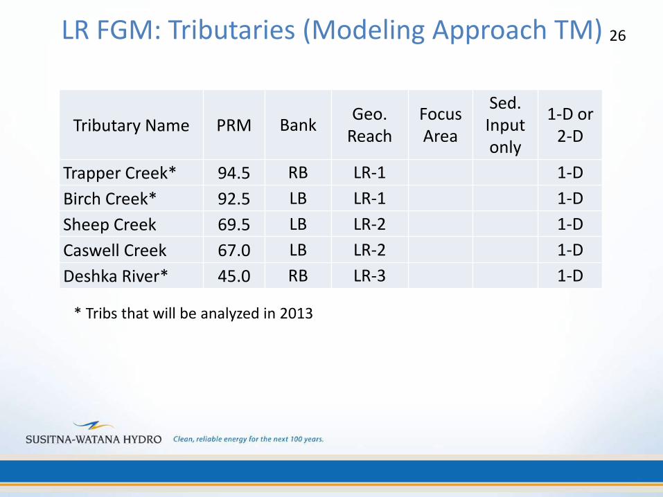
LR FGM: Tributaries (Modeling Approach TM) 26

Tributary Name PRM Bank Geo.

Reach

Focus Area

Sed. Input only

1-D or 2-D

Trapper Creek* 94.5 RB LR-1 1-D

Birch Creek* 92.5 LB LR-1 1-D

Sheep Creek 69.5 LB LR-2 1-D

Caswell Creek 67.0 LB LR-2 1-D

Deshka River* 45.0 RB LR-3 1-D

* Tribs that will be analyzed in 2013

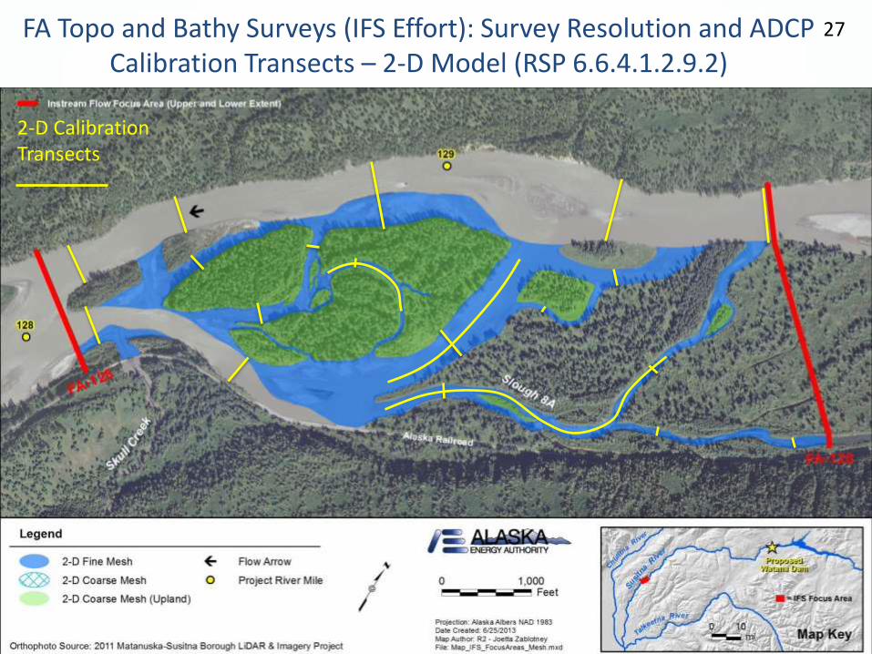
FA Topo and Bathy Surveys (IFS Effort): Survey Resolution and ADCP Calibration Transects – 2-D Model (RSP 6.6.4.1.2.9.2)

2-D Calibration Transects

27

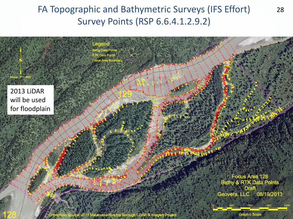
FA Topographic and Bathymetric Surveys (IFS Effort) Survey Points (RSP 6.6.4.1.2.9.2)

2013 LiDAR will be used for floodplain

28

FA Topographic and Bathymetric Surveys (IFS effort) Triangulated Irregular Network (TIN) (RSP 6.6.4.1.2.9.2)

2013 LiDAR will be used for floodplain

29

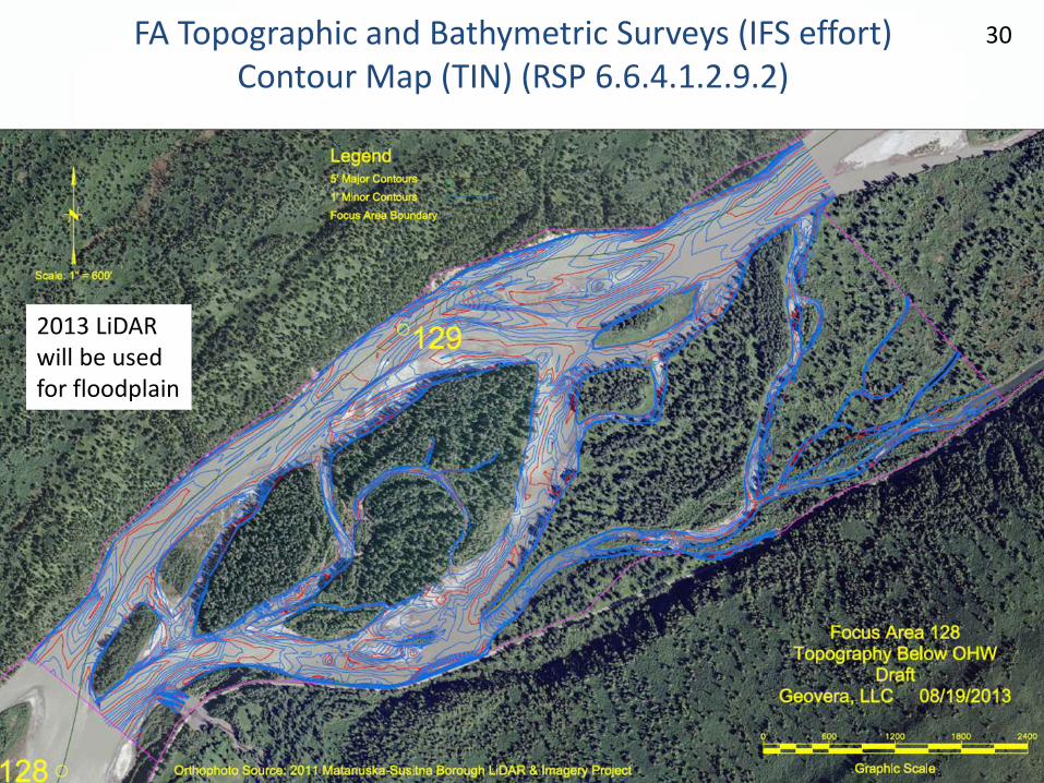
FA Topographic and Bathymetric Surveys (IFS effort) Contour Map (TIN) (RSP 6.6.4.1.2.9.2)

2013 LiDAR will be used for floodplain

30

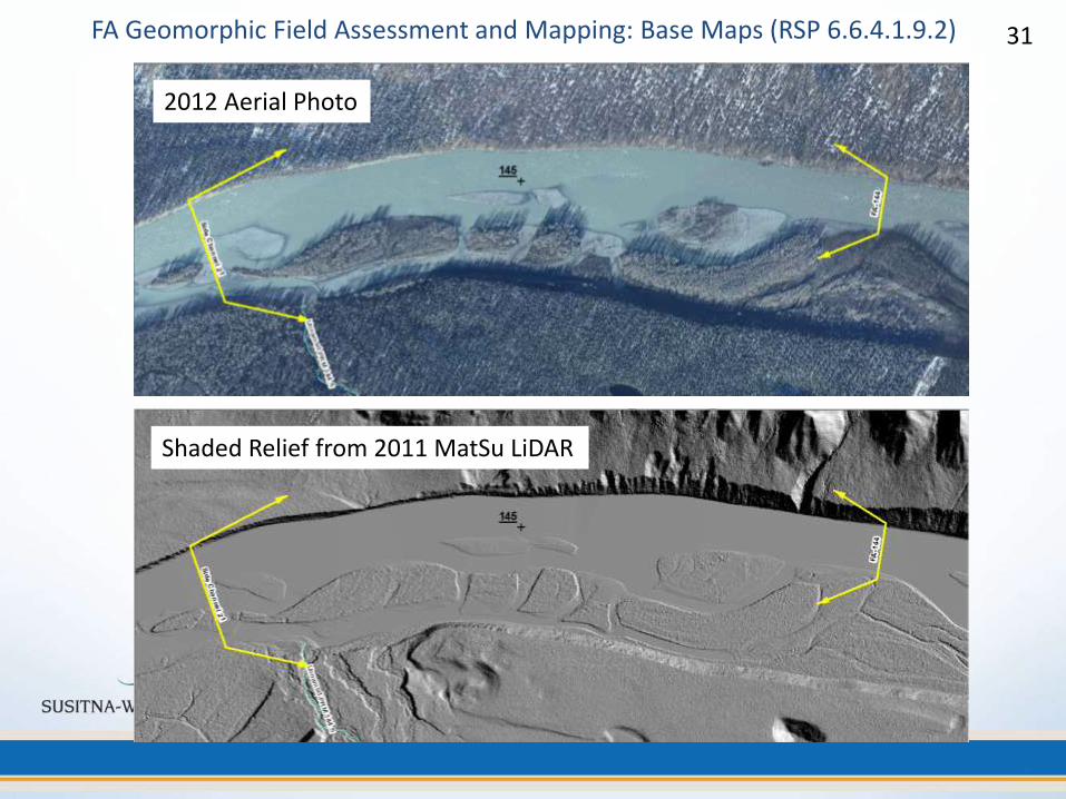
FA Geomorphic Field Assessment and Mapping: Base Maps (RSP 6.6.4.1.9.2)

2012 Aerial Photo

Shaded Relief from 2011 MatSu LiDAR

31

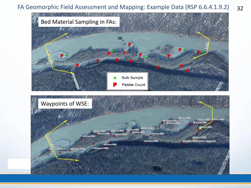
Bed Material Sampling in FAs:

Waypoints of WSE:

FA Geomorphic Field Assessment and Mapping: Example Data (RSP 6.6.4.1.9.2) 32

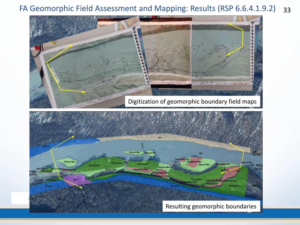
Digitization of geomorphic boundary field maps

FA Geomorphic Field Assessment and Mapping: Results (RSP 6.6.4.1.9.2)

Resulting geomorphic boundaries

33

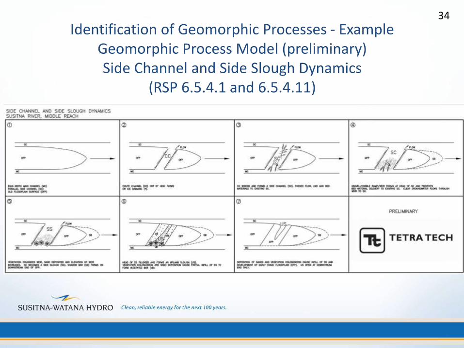
Identification of Geomorphic Processes - Example Geomorphic Process Model (preliminary) Side Channel and Side Slough Dynamics

(RSP 6.5.4.1 and 6.5.4.11)

34

Variance – Collect 2013 LiDAR Rather Than Using 2011 MatSu Borough (RSP 6.6.4.1.2.9)

• RSP indicated 2011 MatSu Borough LiDAR would be used to develop the floodplain portion of the FAs and 1-D cross sections

• Based on LiDAR Verification, decision made to collect higher resolution LiDAR in 2013

35

Variance - Use of LiDAR for Macrohabitat Area: Results and Difficulties with Aerials

(RSP 6.5.4.5 MR and 6.5.6.7 LR) • 2012 could not collect aerials at all target flows

– Flow conditions

– Weather conditions

• Comparison at 12,500 cfs indicated appreciable differences in habitat areas

– Some features shifted classification

• Side channel => side slough

• Side Slough => side channel

– Area changes due to geomorphic processes

36

Variance - Use of LiDAR for Macrohabitat Area: Advantages of LiDAR & Hydraulic Based Approach

(RSP 6.5.4.5 MR and 6.5.6.7 LR)

• LiDAR less susceptible to flow conditions

– Single flight required

• LiDAR less susceptible to weather

– Can penetrate thin cloud cover

– Sun angle not an issue

– Can be flown at night

• Consistent with modeling approach in Focus Areas

37

Large Wood Debris – Variances (RSP 6.5.4.9)

38

• High flow midway through data collection provided additional information on wood transport: – Small debris became mobile at approximately 30,000

cfs at Gold Creek gage; large trees started to move at approximately 40,000 cfs

– Wood in some Focus Areas already inventoried was re-checked after August high flow to determine if wood pieces moved or not

Next Steps • Aerial and LiDAR (RSP 6.5.4.4 and Modeling Approach TM)

• Process information

• Distribute to studies

• Large Woody Debris (RSP 6.5.4.9) • Analyze 2013 field data

• Digitize wood/jams from autumn 2013 aerials if available

• USGS Sediment Transport Data (RSP 6.5.4.2) • Receive 2013 data

• Compare with 2012 and 2013 with 1980s

• Identify need for 2014 data

• 1-D model (RSP 6.6.4.1 and Modeling Approach TM) • Compile and reduce all 2013 field data (RSP 6.6.4.1.2.9.1)

• Develop 1-D tributary models (RSP 6.6.4.1.2.6)

• Initiate 1-D HEC-6T morphology model development (RSP 6.6.4.1.2.5)

• Initial 1-D morphology model run end of Q1 2014 (Modeling Approach TM)

39

Next Steps (Cont.)

• 2-D Morphology Model (Focus Areas) (RSP 6.6.4.1) • Compile and reduce all 2013 field data (RSP 6.6.4.1.2.9.2)

• Develop hydraulic models for FA-104 and FA-128 (Dec 2013) (RSP 6.6.4.1.2.5)

• Develop morphology models for FA-104 and FA-128 end Q1 2014 (RSP 6.6.4.1.2.5 and Modeling Approach TM))

• Final selection of 2-D morphology model , either River2D or SRH-2D end of Q1 2014 (RSP 6.6.4.1.2.1 and Modeling Approach TM)

• Develop Initial Study Report for Geomorphology Study (6.5) and Fluvial Geomorphology Modeling Study (6.6)

40

END

41