Surfactant transport onto a foam film in the presence of surface

viscous stress

Denny Vitasaria, Paul Grassiab,c,∗, Peter Martind

aDepartment of Chemical Engineering, Universitas Muhammadiyah Surakarta,

Jl A Yani Tromol Pos 1 Pabelan Sukarta 57162, IndonesiabDepartment of Chemical and Process Engineering, University of Strathclyde,

James Weir Building, 75 Montrose St, Glasgow G1 1 XJ, UKcDepartamento Ciencias Matematicas y Fısicas, Universidad Catolica de Temuco,

Rudecindo Ortega 02950, Temuco, ChiledSchool of Chemical Engineering and Analytical Science, The Mill, The University of Manchester,

Oxford Road, Manchester M13 9PL, UK

Abstract

Surfactant transport onto a foam film in the presence of surface viscosity has beensimulated as a model for processes occurring during foam fractionation with reflux. Aboundary condition is specified determining the velocity at the end of the film where itjoins up with a Plateau border containing surfactant rich reflux material. The evolutions ofsurface velocity and surfactant surface concentration on the film are computed numericallyusing a finite difference method coupled with the material point method. Results areanalysed both for low and high surface viscosities. Evolution is comparatively rapid whensurface viscosity is low, but the larger the surface viscosity becomes, the slower the surfaceflow, and the lower the surfactant surface concentration on the film at any given time.For a large surface viscosity, the surface concentration of surfactant is maintained nearlyuniform except at positions near the Plateau border where the velocity and surfactantconcentration fields need to adjust to satisfy the boundary condition at the end of thefilm. The boundary condition imposed at the end of the film implies also that a drier foam(i.e. smaller radius of curvature of the Plateau border) leads to less surfactant transportonto the films. Moreover, the shorter the film length is, also the shorter the characteristictime for surfactant transport onto the film surface. Thinner films however give longercharacteristic times for surfactant transport.

Keywords: Foam fractionation; Reflux; Marangoni effect; Interfacial viscosity;Surfactant transfer; Mathematical modelling

1. Introduction

Foam fractionation is an inexpensive and environmentally friendly separation processfor recovering surface active compounds from dilute aqueous solutions [1]. The foam pro-cess is applied for separation of various materials including proteins [1–5], biosurfactants[6–10], microorganisms [11, 12], and other surface active materials [1]. Foam fractionationis usually performed in a fractionation column, gas being sparged from the bottom of thecolumn to create bubbles which form a rising foam. The principle of the separation is

∗Corresponding authorEmail address: paul.grassia@strath.ac.uk (Paul Grassia)

Preprint submitted to Elsevier July 21, 2015

by selective adsorption of a surface active material (hereafter called a ‘surfactant’) to thesurfaces of gas bubbles that are moving towards the top of the column [13].

Some foam fractionation columns are equipped with reflux to increase separation effi-ciency [14–17] by enhancing the enrichment of the foamate. Reflux may be either internalor external [5, 16, 18]. Internal reflux proceeds by in situ bubble coalescence redistributingsurfactant rich material onto films neighbouring those that have recently burst. Exter-nal reflux (the particular situation we study here) proceeds by adding a portion of thecollapsed foamate back to the top of the column: it flows down through the networkof Plateau borders (channels along which three films meet) transporting surfactant toneighbouring films as it flows pasts them. This transport is driven by Marangoni stresses:surfactant-rich Plateau borders, which are fed by reflux material, have lower surface ten-sions than neighbouring surfactant-lean films that are yet to benefit from reflux.

This Marangoni-driven surfactant transfer process has been the subject of a recentstudy [19]. However that study neglected a potentially important interface science effect:Marangoni-driven flows on film surfaces may be opposed by surface viscous effects [20–22].Indeed the surface viscosity of adsorbed monolayers plays a crucial role in the formation,stability and rheology of emulsions or foams as well as in the process of film coating,spraying, flotation and oil recovery [23]. Surface viscosity moreover determines [24] thevelocity profile when surfactant solution flows along a Plateau border in a foam. Whensurface viscosity is high, the flow pattern within the Plateau border is mainly determinedby the bulk viscosity with no slip on the walls of the border. However when surfaceviscosity is low, significant motion on the walls takes place.

Despite the effect that surface viscosity has upon surfactant flows, and despite theimportance of surfactant flows to foam fractionation processes, we are not aware of anyprior studies that have specifically looked at the role of surface viscosity upon fractionationperformance. In an attempt to address this, the present study focuses on modellingthe effects of surface viscosity specifically upon surfactant mass transfer during foamfractionation with reflux. The main focus here is not therefore on flow within Plateauborders [24], but rather on flow on films, as well as flow between Plateau borders andfilms. Our main finding is that surface viscosity reduces (possibly quite substantially)the rate of surfactant transfer onto a film, thereby reducing the efficiency of the refluxprocess during fractionation. The higher the surface viscosity of the surfactant, the longerthe time that films must spend in contact with the Plateau borders in order that refluxmaterial manages to transfer onto the films: this impacts on the residence time for whichfilms must be present in the column. Should residence times turn out to be insufficientfor transfer of a very high surface viscosity surfactant to occur, the fractionation processwould need to be modified e.g. by changing column height and/or changing the rate atwhich bubbles are driven along the column.

This work is laid out as follows. Section 2 introduces the mathematical model of filmsurface velocity with surface viscosity, including the assumptions used and the boundaryconditions assigned. This same section also introduces the mathematical model governingsurfactant concentration on the film. Section 3 discusses the challenges involved in quan-tifying surface viscosity and the variability in reported measurement results. Section 4presents simulation parameters selected for our model. The numerical solution method-ology is presented in Section 5. The numerical results of the time evolution of surfacevelocity and surfactant surface concentration are discussed in Section 6. Conclusions arepresented in Section 7.

2

2. Mathematical model of the surface velocity

Deformation of the surface of a foam film leads to surface stresses [20, 25]. Thosesurface stresses can be an elastic stress or viscous stress or both. The viscous stress canoriginate from shear deformation and dilational deformation of the film surface itself,while the elastic stress originates from dilation of the film surface, and is characterised bya Gibbs elasticity parameter. The surface shear and surface dilational viscous stresses (perunit strain rate) are characterized by constants called respectively surface shear viscosityand surface dilational viscosity. For a particular mode of surface deformation that involvesspecified amounts of both surface shear and dilation (as e.g. in the specified geometryto be considered below), these constants can be combined together into a single surfaceviscosity parameter.

A mathematical model of the velocity within the bulk of a foam film and on its surfaceis developed below: a 2-D bulk flow field and 1-D surface flow are considered (Figure 1).For simplicity, we study a 2-D bulk field rather than e.g. an axisymmetric one here. Indry foams at least, foam films tend to be polygonal rather than circular, so switching to anaxisymmetric field would add complexity but still not be perfectly accurate geometrically.

This section is laid out as follows. Subsection 2.1 describes the assumptions takento develop the model, while Subsection 2.2 introduces the equations for surface velocity.Subsection 2.3 presents a key parameter influencing the model behaviour, while Subsec-tion 2.4 describes the boundary conditions associated with the surface velocity profile.Finally Subsection 2.5 discusses the surfactant conservation equation, which coupled tothe surface velocity profile, determines the rate of evolution of surfactant concentration.

2.1. Assumptions of the model

The mathematical model of surface velocity in this study is developed based on thefollowing assumptions:

• At initial time, the surface concentration of surfactant along the film is uniform.

• The surface concentration of surfactant on the Plateau border is fixed all the time tothe value set by the reflux to the foam fractionation column. This is higher than theinitial surface concentration on the film. Whilst it is possible in principle to general-ize to the case where the surfactant concentration in the Plateau borders graduallydecreases as material is transferred across to the films, this is a complication wehave chosen to ignore here. What matters for driving flow is the surfactant con-centration difference between borders and films, and this concentration differencedecreases with time as the film surfactant concentration rises, even when changesin the Plateau border concentration are ignored.

• The liquid in the film is incompressible and Newtonian. The film surface is howeverviscoelastic, supporting both surface viscous stress and elastic Marangoni stress.

• The film is taken to be flat and has uniform thickness along its length [19, 26,27]. Moreover liquid drainage from films is ignored, so film thicknesses are heldconstant with time. These assumptions are mathematically convenient, as theygreatly simplify the flow fields we need to compute. It should be mentioned howeverthat foam films are known to develop non-uniform, dimpled shapes [28–30], whilstfilm drainage tends to oppose Marangoni-driven surfactant motion from surfactant-rich Plateau borders to surfactant-lean films [19].

3

• The thickness of the film is much smaller than its length, consequently the associatedReynolds number, with length scale based on the film thickness, is very small [31]and a lubrication approximation is assumed [32–38].

• The Plateau border, which has a tricuspid shape, has a characteristic size that isintermediate between the film length and the film thickness, but may well containrather more liquid than the exceedingly thin films.

The mathematical model for evolution of surfactant surface concentration (developedby [19] and to be employed in what follows) utilises the following additional assumptions.

• Films are sufficiently thin (or equivalently surfactant solubility is sufficiently low)that the surface excess of surfactant dominates any surfactant in solution in the bulkof the film. In other words, even if surfactant manages to diffuse from film surfacesacross their bulk [33], the surfactant that is ‘lost’ from the surface is insignificantcompared to the overall surfactant budget. Recall also that film drainage is ignoredfrom our model, as was stated previously. Were film drainage to be present however,any material that diffuses from the film surface to the film interior, would in principlebe advected by the film drainage velocity field back towards the Plateau border,leading to quite a complex transport process overall that we choose to neglect here.

• Marangoni-driven surfactant flows along surfaces are much faster than surfactantdiffusion along surfaces.

2.2. Governing equations

The equation for the profile of surface velocity taking into account the surface viscosityis developed based on lubrication theory and driving Marangoni-stresses. The equationgoverning the profile of the surface velocity (which can be obtained from a generalisationof a procedure outlined by [19], and which involves a straightforward balance betweenthe viscous shear stress immediately below the surface and the gradient of surface elastictension and surface viscous tension along the surface) turns out to obey [39]:

us =δ03µ

[

∂γ

∂x+

∂

∂x

(

µs∂us

∂x

)]

(1)

where us is the surface velocity, x is the distance from the centre of the film along itslength, δ0 is the half thickness of the film, µ is the liquid viscosity, γ is the surface tension,µs is the surface viscosity.

We use a simple Gibbs elasticity model [40] to convert between surface tension γ andsurfactant surface excess Γ:

dγ/d ln Γ = −G (2)

where G is a Gibbs parameter that we take to be a constant. This captures the tendencyof γ to decrease as Γ increases, but represents nonetheless a considerable simplificationof the true relation between γ and Γ (contrast e.g. the much more complicated relationsin [41]). Equation (2) was used in [19] because it leads to a convenient linear relationbetween surfactant concentration gradient and surfactant flux, giving (in the absence ofsurface viscosity) a linear partial differential equation for the spatio-temporal evolutionof Γ. We adopt the same model here to facilitate comparison between results with andwithout surface viscosity.

4

We deduce

us =δ03µ

[

∂

∂x

(

−G lnΓ

ΓPb

)

+∂

∂x

(

µs∂us

∂x

)]

(3)

where ΓPb is the (fixed) surface excess of surfactant on the surface of the Plateau border.This is larger than the surface excess on the film (Γ or ΓF0 initially at time t = 0). Theright hand side of equation (3) represents a Kelvin-type viscoelastic model for a foamfilm surface, and corresponds to what was done by [40]. We note however that there arecompeting Maxwell-type viscoelastic models in the literature [42, 43].

A dimensional analysis was carried out upon equation (3) and results in:

u′

s = −1

3

∂ ln Γ′

∂x′+

δ′0µs

3

∂2u′

s

∂x′2. (4)

where u′

s = usµ/Gδ′0 is the dimensionless surface velocity, δ′0 = δ0/L is the dimensionlesshalf film thickness, δ0 is the half film thickness, L is half of the film length, x′ = x/L isthe dimensionless distance from the centre of the film along its length, Γ′ = Γ/ΓPb is thedimensionless surface excess of surfactant and µs = µs/µL is the dimensionless surfaceviscosity. The dimensionless surface viscosity is the reciprocal of the surface mobilityparameter identified in previous studies [24, 44].

2.3. Role of the parameter δ′0µs

The parameter δ′0µs is important in equation (4) since it determines the effect ofsurface viscosity upon the system (an estimated value for this parameter will be providedshortly). If δ′0µs is small, the effect of surface viscosity is weak, and the equation of thesurface velocity profile can be simplified as follows:

u′

s = −1

3

∂ ln Γ′

∂x′(5)

which indicates that film surface velocity is driven by Marangoni effects [19], any surfaceviscous effects being neglected.

Note a significant difference between equation (4) and (5). Whereas the former equa-tion is a second order differential equation in space (and so the velocity field can only bedetermined given suitable boundary conditions, which we will consider in Subsection 2.4),the latter gives the velocity u′

s directly once the surfactant concentration field Γ′ vs x′ isknown. There is no guarantee in this case that boundary conditions on u′

s will be met.This then indicates that even in the limit of small δ′0µs, the velocity field might need

to deviate away from equation (5) in boundary layers. Equation (4) implies that the char-acteristic thickness of these boundary layers must be order (δ′0µs)

1/2, since for a boundarylayer on that length scale, the nominally ‘small’ surface viscous term in equation (4)namely 1

3δ′0µs ∂

2u′

s/∂x′ 2 becomes comparable with the other two terms in that equation.

Further discussion about these boundary layers can be found in the appendix.On the other hand, if δ′0µs is very large, there is balance between the Marangoni effect

and surface viscosity, and it turns out that u′

s ≪ 1. In this limit it is convenient to rescalethe velocity, i.e. to define u′′

s such that u′′

s = δ′0µs u′

s (or equivalently u′′

s = usµs/GL) sothat equation (4) becomes

3u′′

s

δ′0µs= −

∂ ln Γ′

∂x′+

∂2u′′

s

∂x′2. (6)

5

As a result, for δ′0µs ≫ 1, we can simplify into the following equation:

∂2u′′

s/∂x′ 2 = ∂ ln Γ′/∂x′. (7)

Equation (7) indicates that the total film tension which consists of the Gibbs-Marangoniand surface viscosity contributions is spatially uniform when δ′0µs is very large. It turnsout that the solution of equation (7) for u′′

s can be expressed in terms of an integral overln Γ′ as is described in the appendix. Nonetheless equation (7), like equations (4) and (6),can however only be solved uniquely given suitable boundary conditions.

The determination of the boundary condition is presented in the following subsection.

2.4. Boundary conditions

The surface velocity u′

s must vanish midway along the film (i.e. at x′ = 0) on symmetrygrounds. In addition, due to symmetry on the Plateau border, the value of u′

s must alsofall to zero at the ‘symmetry point’ of a tricuspid Plateau border (see Figure 2). The‘symmetry point’ is the midpoint of the curved section of each tricuspid arc. Since eachof the tricuspid curves subtends an arc π/3, the angle subtended between the cusp andthe symmetry point is π/6, making the distance (measured along the film) between thecusp and the midpoint be L′

Pb = a′π/6, where a′ = a/L is the dimensionless radius ofcurvature of the Plateau border and a is the radius of curvature of the Plateau border.We can also think of the parameter a′ as being connected with the liquid fraction of thefoam [45]: the volume of liquid contained in the Plateau borders around a bubble relativeto the bubble volume itself scales proportional to a′ 2.

We can take the (dimensionless) distance from the centre of the film to the ‘symmetrypoint’ of a tricuspid Plateau border (measured along the surface) as 1 + a′π/6. Onsymmetry grounds, the velocity component along the surface accelerates away from thethe symmetry point where it vanishes (or equivalently decelerates towards the symmetrypoint). Surface viscosity couples the motion of nearby points to one another: given thecomparatively small size of the Plateau border (compared to the film length), pointstowards the end of the film may well be influenced by the fact that the symmetry point ofthe Plateau border remains stationary. In particular, if the surface viscosity is large, thefact that the velocity component must be zero at the symmetry point will couple back tothe film, keeping the surface flow very small especially at the end of the film. Moreoverthe drier the foam (i.e. the smaller the value of a′) the more strongly the end of the filmis coupled to the stationary Plateau border symmetry point, and the less the permittedsurfactant transfer onto the end of the film.

The surface of the tricuspid Plateau border is of course a complicated 2-D shape. Asa simplifying approximation, we unfold it into a 1-D line. By ‘uncurling’ the surface ofthe tricuspid Plateau border, we simplify the geometry as well as the mathematics butstill capture the essential physics of the flow accelerating away from the symmetry point(or equivalently decelerating towards the symmetry point).

Two boundary conditions are required to solve the differential equation (4). Oneboundary condition is at x′ = 0 where we have u′

s|x′=0 = 0. The other boundary conditionis taken at x′ = 1 by imposing the constraint at the symmetry point of a tricuspid Plateauborder and supposing that u′

s is nearly linear in x′ over the domain 1 < x′ < 1+a′π/6 (i.e.the surface velocity decelerates uniformly between the end of the film and the symmetrypoint of the Plateau border). Therefore, the boundary condition at the end of the film

6

near the Plateau border is as follows:

∂u′

s

∂x′

∣

∣

∣

x′=1=

0− u′

s|x′=1

a′π/6(8)

rearranging to:

u′

s|x′=1 +a′π

6

∂u′

s

∂x′

∣

∣

∣

x′=1= 0. (9)

The velocity boundary condition at the end of film in equations (8) and (9) is shiftedto x′ = 1 instead of at the symmetry point itself at x′ = 1+a′π/6. The reason for shiftingthe boundary condition in this fashion is that the fluid flow and the surfactant masstransfer model that we analyse considers only the domain of the film (i.e. 0 < x′ < 1)without any detailed model for the Plateau border (1 < x′ < 1+a′π/6). The detailed flowfield in the Plateau border itself is very complex – with flow changing direction withinthe border – and it is beyond the scope of this study.

Having a boundary condition at x′ = 1 is also convenient when solving the massconservation equation for surfactant (since Γ′ only needs to be computed in the domain0 < x′ < 1) and one can simply assume that surfactant coverage on the Plateau borderis fixed. This follows because typically, the bulk of the liquid in a foam is in the Plateauborders (meaning that the Plateau border surfaces can continually be replenished bysurfactant arriving from the interior of the borders). This does not contradict the notionof the surfactant being nominally ‘low solubility’ which only requires that surfactant bepresent primarily as surface excess on the length scale of the (exceedingly thin) films.

According to equation (9) the velocity at the end of the film, u′

s|x′=1 can be affectedby the parameter a′, which is normally quite a small parameter (being the ratio betweenthe length scale of the Plateau border cross section and the length scale along the films).

Recall however that when the parameter δ′0µs ≪ 1, the velocity field both near x′ = 0and near x′ = 1 is potentially affected by boundary layers, the relevant boundary layer sizebeing order (δ′0µs)

1/2. In practice no boundary layer arises near x′ = 0, the reason beingthat ∂ ln Γ′/∂x′ vanishes there on symmetry grounds, and equation (5) then predicts thecorrect boundary condition u′

s|x′=0 = 0 even with vanishing surface viscosity. A boundarylayer does however arise near x′ = 1. In fact, very different behaviour is expected accordingto whether the boundary layer size of order (δ′0µs)

1/2 is lesser or greater than the distanceπa′/6 to the symmetry point of the Plateau border. The reasons for this are as follows.

In the case where the boundary layer size is much less than the distance to the bordersymmetry point, i.e. (δ′0µs)

1/2 ≪ πa′/6, the boundary layer is effectively unaware of theconstraint imposed by the Plateau border symmetry point, and so a comparatively largevelocity is permitted at x′ = 1 transferring surfactant from Plateau border to film. Onthe other hand, when (δ′0µs)

1/2 ≫ πa′/6, the boundary layer on the film is well awareof the constraint arising from the Plateau border symmetry point, and (as a result) thesurfactant velocity at the end of the film is substantially reduced. Further details of thissituation can be found in the appendix.

This completes our model of the surface velocity field on a foam film in the presenceof surface viscosity. This surfactant velocity field then advects the surfactant causing thesurfactant concentration to change: this process is considered in the next subsection.

2.5. Evolution of surfactant concentration

As in previous work [19], we adopt the following conservation equation for the evolu-tion of surfactant surface concentration or excess (which is itself a special case for a flat

7

interface of a more general equation considered by [46])

∂Γ′/∂t′ + ∂(Γ′u′

s)/∂x′ = 0. (10)

Here t′ is a dimensionless time related to dimensional time t via t′ = tGδ′0/Lµ. Clearlyequation (10) is a partial differential equation for Γ′ to be solved along with the ordinarydifferential equation (4) governing u′

s. The technique for solving this equation will bediscussed later on in Section 5, but for the moment we just make some brief remarks.

In the limit when δ′0µs ≫ 1, we have already discussed how we can rescale dimen-sionless velocity (with rescaled velocity u′′

s equal to δ′0µs u′

s). In a similar fashion we canrescale time, with rescaled time t′′ defined as t′′ = t′/(δ′0µs), implying that t′′ = tG/µs.The form of equation (10) then remains unchanged provided we replace t′ by t′′ and u′

s byu′′

s . Remember also (as commented in Subsection 2.3) that in the limit as δ′0µs ≫ 1, thevelocity field u′′

s can be obtained in terms of an integral of ln Γ′. If this is substituted intothe surfactant conservation equation we have an integro-differential equation for ln Γ′.

Whether we adopt the differential equation formulation of equation (10) (for finiteδ′0µs) or the integro-differential equation formulation (for δ′0µs ≫ 1) we need to supplyinitial and boundary conditions for dimensionless surfactant concentration Γ′. Initiallythe surfactant concentration is assumed to be uniform, Γ′ = Γ′

F0 where Γ′

F0 is a dimen-sionless constant (being the ratio between the dimensional concentrations ΓF0 and ΓPb

respectively on the film and Plateau border). Here Γ′

F0 is smaller than unity, since inthe process of foam fractionation with reflux, comparatively surfactant-lean films con-tact comparatively surfactant-rich Plateau borders. The boundary condition meanwhileis that the dimensionless surfactant concentration at the point x′ = 1 at the end of thefilm satisfies Γ′|x′=1 = 1 for all times t′ > 0. In other words the dimensional surfactantconcentration at the end of the film matches the surfactant concentration on the Plateauborder. Note that (as has already been mentioned in Subsection 2.4) at the midpoint ofthe film x′ = 0 a symmetry condition ∂Γ′/∂x′|x′=0 = 0 also applies, but we do not need toimpose this explicitly: it arises naturally from the symmetries of the governing equations.

This completes our formulation of the model for evolution of surfactant concentration.However in order to compute with the model we require values of model parameters, inparticular values for the relevant surface rheological material properties. Unfortunatelyhowever these are not always readily obtained (as we explain in the next section).

3. Variability of measurements of surface viscosity

Measuring surface viscoelastic properties is very challenging since those properties areaffected by environmental contamination [47]. Moreover, it is not always easy to distin-guish between surface elasticity and surface viscosity [47], and, as a possible consequence ithas been observed that different experimental methods to determine the surface viscosityresult in measured values of surface viscosity differing by orders of magnitude [47–49]. Fur-thermore foam fractionation (our target application) is often employed as a technique forpurifying proteins, but proteins can exist in many conformational states at surfaces [50],each state having different viscoelastic properties. Indeed the conformational state (andhence the viscoelastic properties) can change during the course of an experiment.

In this study we will use as a ‘base case’ a value for surface viscosity of bovine serumalbumin (BSA) together with a cosurfactant propylene glycol alginate (PGA) as reportedby [40]. We note however that for the common surfactant SDS the particular measurementtechnique of [40] determined surface viscosity values 5 orders of magnitude higher than

8

measurements on SDS performed by other authors [49]. Hence it is possible to speculatethat the surface viscosity reported by [40] for BSA/PGA could be likewise too high.

The study of [40] also provided our ‘base case’ value of the half film thickness δ0.That study ignored film drainage, whereas a fully drained ‘common black’ film (halfthickness denoted δcb) would have a thickness orders of magnitude smaller than our basecase thickness value.

We already commented (Subsection 2.3) how the effect of surface viscosity appearsas a product δ′0µs, the parameter δ′0 being dimensionless half film thickness and µs beingdimensionless surface viscosity. The effect of possibly having a dimensionless surfaceviscosity orders of magnitude smaller than our ‘base case’ is achieved analogously in whatfollows by reducing the dimensionless film thickness, thereby replacing the non-drainingfilm of [40] by a much thinner one that is substantially closer to a common black film.

4. Parameters for simulation

Typical parameter values for the simulation are presented in Table 1 while the relevantdimensionless parameters are presented in Table 2.

All parameters except the values of ΓPb, ΓF0, δcb, δ0 and a were taken from [40] usingprotein BSA together with a cosurfactant PGA, both at concentration of 4.0 g L−1. Thevalue of a was estimated as presented in [19], while the value of δcb was taken from [45].The values of ΓPb, ΓF0 are estimates, taken as lower than the maximum surface excessΓmax of BSA which was reported in a study by [51] to be Γmax = 5× 10−8 mol m−2. Wereiterate these are base-case parameter values and variations about the base case will beconsidered in the simulations.

The quantity δ′0µs is the key parameter to determine the effect of surface viscosityupon the system. Using the base-case parameters presented in Table 1, the value ofthat key parameter is δ′0µs = 3.5 ± 1.4. However, as already mentioned there is a lot ofuncertainty associated with this parameter, with the possibility of much smaller valuesbeing relevant. Under such circumstances, it is useful to understand how the systembehaves in the limiting cases of small and large values of this parameter. This is achievedin Section 6, starting first of all with small δ′0µs and then progressing onto large δ′0µs.

In the first instance we have elected to access small δ′0µs values, via keeping µs fixed(at the base case value of 886 given in Table 2), whilst reducing δ′0, specifically taking theδ′0 value to be 6× 10−5, intermediate between δ′cb (namely 3× 10−6, the smallest allowedvalue as mentioned in Table 2), and the base case δ′0 (which is 4× 10−3 in Table 2). Theresulting value of δ′0µs is now 5.4 × 10−2 and so is significantly smaller than unity. Oneconsequence of reducing film thickness (it is now 66 times smaller than the base case) isthat we also increase the characteristic time scale shown in Table 1 by the same factor:instead of being 0.134 s, it is now close to 9 s.

To access a large δ′0µs we have decided to retain the same δ′0 value as just discussedabove (namely 6 × 10−5) but to increase µs by two orders of magnitude (from the basecase µs value of 886, to a new value of 8.86 × 104). The resulting δ′0µs is now slightlylarger than the base case value quoted in Table 1, specifically δ′0µs now equals 5.4 insteadof the base case value 3.5.

The parameter ranges used specifically in these small and large δ′0µs computations arepresented in Table 3. The base case a′ value is a′ = 0.1. Most of our computations aredone for this value, but a small number of them will be done for a′ = 0.25 correspondingto a wetter foam. The parameter Γ′

F0 is fixed at 0.5, i.e. only half as much surfactantconcentration on the film surfaces initially as on the Plateau borders.

9

We reiterate that the key parameter here is δ′0µs which according to Subsection 2.3affects the velocity field u′

s and/or u′′

s , and this in turn influences the evolution of Γ′.Our main aim here is to determine how δ′0µs affects surfactant transport by solving thegoverning equations numerically. Additional insight into the role of this δ′0µs parametercan however be gained by obtaining analytical expressions for u′

s and/or u′′

s for givensimple analytical forms of Γ′: these are taken up in the appendix. The simple analyticalforms of Γ′ might only apply for a restricted set of times, since Γ′ is continually evolving.The velocity fields one determines are nevertheless instructive as the appendix explains.

5. Numerical solution technique

The numerical solution technique for equation (10) follows a material point methodused by [19]. We outline the method briefly here, but readers should refer to [19] formore details. Discrete material points are distributed along the foam film surface andalso (in the specific case of a foam fractionation column with reflux) where the filmmeets a surfactant rich Plateau border. Velocities of each material point are computed,in the present case incorporating surface viscosity by a finite difference method appliedto equation (4). The material point positions change on every time step, leading touneven spatial intervals over time. To keep the spatial intervals even, a bookkeepingoperation is applied at the end of every time step to restore equal width intervals: thisthen recovers second order spatial accuracy for the numerical scheme. The mechanismof the bookkeeping operation is similar to the one reported in the previous study [19].Moreover the temporal accuracy of the numerical simulation is improved using a predictor-corrector method namely Heun’s method [52, 53].

The system is discretised [54] into I+1 spatial (material) points, i.e. I spatial intervals,and N time steps. Values of I ranged between 200 and 250, whilst values of N rangedbetween 10000 and 20000. In the case of a small δ′0µs, specifically δ′0µs = 5.4 × 10−2, wechose I = 250 giving a spatial interval ∆x′ = 4 × 10−3. Moreover we chose N = 20000and integrated to t′ = 2 (corresponding to a time step ∆t′ = 10−4). In the case of a largeδ′0µs, specifically δ′0µs = 5.4, we chose I = 200 giving a spatial interval ∆x′ = 5 × 10−3.Moreover we chose N = 10000 and integrated to a rescaled time t′′ = 20 (correspondingto a time step ∆t′′ = 2× 10−3).

In addition to the above, we performed a number of convergence tests, includingdoubling the number of spatial steps and/or halving the number of time of steps, andlooking at the root mean square of differences in predicted Γ′ vs x′ profiles at either t′ = 2or t′′ = 20 This resulted in a root mean square difference of 2× 10−3 (or less) comparingcoarser vs finer spatial grids, and a root mean square difference of 10−4 (or less) comparingcoarser vs finer temporal grids.

Recall (from Subsection 2.5, and also the appendix) that for δ′0µs ≫ 1 we can replacethe differential equation (10) by an integro-differential equation. We solved this on a fixed(Eulerian) grid with I = 200 spatial intervals and N = 20000 time steps out to t′′ = 20.

Typical run times for our programs were on the order of a few minutes. Results fromthese programs are presented in Section 6 below.

6. Evolution of surface velocity and surfactant surface concentration

In what follows numerical results are presented for velocity and surfactant surfaceconcentration fields. Bearing in mind the different behaviours expected between the casesδ′0µs ≪ 1 and δ′0µs ≫ 1, we treat these two cases in turn. Subsection 6.1 presents

10

the evolution of surface velocity and surfactant surface concentration in the case whereδ′0µs is significantly smaller than unity, specifically δ′0µs = 5.4 × 10−2. Subsection 6.2deals with the case where δ′0µs is significantly larger than unity, specifically δ′0µs = 5.4.Subsection 6.3 discusses the effects of considering different film lengths.

6.1. Evolution in the case where δ′0µs ≪ 1

Data shown in this subsection have δ′0µs = 5.4× 10−2, a′ = 0.1 and Γ′

F0 = 0.5.Surface velocity profiles are presented in Figure 3. At early times, velocity is near

zero far from x′ = 1, as velocity profiles are sharply peaked near x′ = 1. The maximumsurface speed occurs very slightly to the left of x′ = 1 however, due to a need to meet thevelocity boundary condition at x′ = 1. At later times the velocity distributions are morespread out and the peak speeds are less.

The corresponding surface concentration of surfactant is presented in Figure 4. Overtime the surfactant concentration grows and the surfactant concentration profile becomesincreasingly spread out. For comparison the evolution of surfactant surface concentrationin the absence of surface viscosity is presented in Figure 5. Comparing the surface con-centrations calculated in the presence of surface viscosity and in its absence, it appearsthat surfactant transport onto the foam film is slower in the case with surface viscosity.At early time, the growth of surfactant surface concentration obtained using the modelwith surface viscosity is actually much slower than that obtained using the model with-out surface viscosity. The mass of surfactant transferred in fact grows like square root oftime in the absence of surface viscosity [19], but only linearly in time in the presence ofsurface viscosity (because surface viscosity keeps the film velocity finite even for an arbi-trarily sharp gradient of surfactant concentration). At later time, the relative differenceof surface concentration obtained using those two models becomes smaller.

The spatially-averaged surfactant surface concentration over time with surface vis-cosity can be compared with that in the case without surface viscosity and the result ispresented in Figure 6. In the case without surface viscosity, at early time, the rate ofaccumulation of surfactant on the surface of the film is faster than that in the case withsurface viscosity. This is shown by the steep increase of surface concentration at earlytime for the case without surface viscosity. In the case with surface viscosity, this earlytime growth is moderated by the surface viscous effect. At later time, the rate of accu-mulation of surfactant on the surface of the film slows down, and the predictions in thepresence and absence of surface viscosity are similar (albeit with slightly less surfactanttransferred in the former case).

6.2. Evolution in the case where δ′0µs ≫ 1

In the case where δ′0µs ≫ 1, it is convenient to rescale the dimensionless velocity andtime as described in Subsections 2.3 and 2.5. The rescaled equations are solved eithervia finite differences with the material point method (see Subsection 6.2.1) or via anintegro-differential equation (see Subsection 6.2.2). Subsection 6.2.3 considers analyticapproximations to the solutions, whilst Subsection 6.2.4 contrasts large vs small δ′0µs.

6.2.1. Solution using finite difference method for the case of δ′0µs ≫ 1

This subsection presents results for the case where δ′0µs = 5.4, a′ = 0.1 and Γ′

F0 = 0.5.The profiles of surface velocity obtained are presented in Figure 7. It is clear that

gradients of surface velocity are nearly spatially uniform away from x′ = 1. This is infact the behaviour expected (see the appendix). At early time, the magnitude of u′′

s

11

(in this region away from x′ = 1) grows. If the width of the region near x′ = 1 overwhich the surfactant concentration deviates from uniformity grows, the magnitude of∂u′′

s/∂x′ (and hence of u′′

s itself) outside this region also grows, again as predicted inthe appendix. At later times however, the magnitude of ∂u′′

s/∂x′ decays, since gradients

of surface concentration eventually decay as surfactant accumulates on the film surface,implying that the Marangoni forces which ultimately drive the flow field become weaker.

Near the end of the film, the surface velocity profile deviates from a straight line tosatisfy the x′ = 1 boundary condition. The magnitude of surface velocity right at the endof the film x′ = 1 turns out to be a decreasing function of time (see the inset in Figure 7).

Profiles of surfactant surface concentration are presented in Figure 8. As anticipatedin the appendix, the surface concentration of surfactant is uniformly distributed along thefilm except at positions near the Plateau border. The uniform concentration region doesseem to shrink in size between times t′′ = 0 and t′′ = 4 but then starts growing again.

We can rationalise this observation as follows. The non-uniform concentration regionnear the Plateau border tends to invade the uniform region further away when there ismore surfactant flux entering the film from the Plateau border at x′ = 1 than enteringthe uniform region slightly to the left of x′ = 1. Conversely the uniform region tends toexpel the non-uniform region back towards the Plateau border when the surfactant fluxentering the film from the Plateau border at x′ = 1 is less than that entering the uniformregion slightly further to the left.

The magnitude of the surfactant flux is the product Γ′|u′′

s |, remembering u′′

s < 0 here.As we move leftwards from x′ = 1, the value of Γ′ falls, and this tends to reduce the surfac-tant flux, in turn giving a tendency for the non-uniform concentration region to grow andthe uniform region to shrink. Counterbalancing this, again moving leftwards starting fromx′ = 1, the magnitude of |u′′

s | grows moving across the non-uniform concentration regiontowards the uniform one, tending to increase the surfactant flux: this favours shrinkageof the non-uniform region at the expense of growth of the uniform one. Concentrationgradients in the non-uniform region must sharpen as the region itself shrinks1.

When the non-uniform concentration region is highly compact, the change in |u′′

s | isnegligible moving leftward from x′ = 1 across the non-uniform region. The dominanttendency affecting the spatial variation of the surfactant flux is therefore that due to thechange in Γ′, and hence the non-uniform concentration region grows at the expense of theuniform one. As the size of the non-uniform concentration region grows however, moresubstantial changes in |u′′

s | can occur moving leftward from x′ = 1 across the non-uniformregion up to the edge of the uniform one. These changes in |u′′

s | now dominate the spatialvariation of the surfactant flux. This then permits the uniform concentration region togrow at the expense of the non-uniform one.

6.2.2. Calculation of surfactant surface concentration via an integro-differential equation

We now describe results obtained via the integro-differential equation as detailed inthe appendix. As in Subsection 6.2.1, we have a′ = 0.1 and Γ′

F0 = 0.5, but we now haveformally δ′0µ → ∞ instead of δ′0µ = 5.4 as was the case for Figure 7–Figure 8.

1Note that this mechanism sustaining sharp gradients of surfactant concentration really only relieson relative variations in u′

s exceeding relative variations in Γ′, and does not demand large δ′0µs, eventhough we have discussed it in that particular context. An analogous mechanism could also be active inthe case of small δ′0µs, as the sharpness of the surfactant concentration gradients near x′ = 1 in Figure 4(compared to Figure 5) indeed suggests.

12

Integro-differential equation surfactant concentration profiles results are presented inFigure 9. They are remarkably similar to those of Figure 8 even though one set of results(finite difference) was determined for δ′0µs = 5.4 and the other set (integro-differentialequation) formally for δ′0µs → ∞. This close similarity is also reflected in the spatially-averaged surfactant surface concentration plotted vs time in Figure 10. To quantify thedifferences in the spatially-averaged data between the finite δ′0µs cases compared to thecase where δ′0µs → ∞, we evaluated the root mean square difference of the spatially-averaged data between times t′′ = 0 and t′′ = 20. This root mean square difference was0.0013 for δ′0µs = 5.4, rising to 0.0031 for δ′0µs = 2.7 and to 0.0168 for δ′0µs = 0.54.

6.2.3. Comparison with approximate analytic solution

Using the assumption of near uniform surfactant surface concentration over (almostall of) the film, the evolution of surfactant surface concentration in the uniform regioncan be predicted using equation (A.10) given in the appendix.

In Figure 11, predictions from equation (A.10) are compared with the finite differenceand integro-differential equation computations. In this figure, the data is only presentedup to two units of time to show the agreement of the results of the three methods for calcu-lation of Γ′ at x′ = 0. At very early times equation (A.10) agrees with the finite differenceand/or integro-differential equation results. At later time, the predictions obtained usingequation (A.10) deviate from the two other methods. This is because equation (A.10)assumes an arbitrarily abrupt jump in surfactant surface concentration at the end of thefilm, whereas in reality the concentration changes over a thin but finite region. Note thataccording to the numerical predictions the growth rate of surfactant surface concentrationat x′ = 0 increases over time as the region where the profile of Γ′ vs x′ departs from uni-formity grows, and this must be associated with increases in the magnitude of the surfacestrain rate |∂u′′

s/∂x′| in those parts of the domain where Γ′ remains uniform.

6.2.4. Comparison of large and small surface viscosity cases

Our data for large δ′0µs have been expressed in terms a rescaled time t′′ instead of t′.Given that t′ = δ′0µs t

′′, clearly our large δ′0µs data consider time scales much longer thanthose studied with a smaller surface viscosity parameter. To effect a comparison betweenthe small and large δ′0µs data, we convert the latter back into the original t′ scaling. Theresult for spatially-averaged surfactant surface concentration is presented in Figure 12. Itis clear that the rate of surfactant transport onto the film surface is much slower for largesurface viscosity compared to the small surface viscosity case.

Just how slowly this large δ′0µs case evolves for the current set of parameter values canbe appreciated by referring to Figure 10 which indicates that the surfactant concentrationon the film has only proceeded about half way to equilibrium with the Plateau border evenby t′′ = 10 (or equivalently by t′ = 54 since δ′0µs = 5.4 here). Remember from Section 4that 1 unit of dimensionless time t′ corresponds to roughly 9 s (this is longer than the scale0.134 s quoted in Table 1 because we are assuming a substantially smaller film thicknessas Section 4 explains). It follows that, in a foam fractionation column operated withreflux, to equilibrate a high surface viscosity film with surfactant rich reflux material inPlateau borders, we may need to ensure that the contact time between the film and thePlateau borders is hundreds of seconds long2. Strategies for increasing this contact time

2In fact the reason that such a long time scale results here is that we have chosen a value of µs =8.86 × 104 which is 100 times bigger than the base case value quoted in Table 1. Each unit of rescaled

13

(or equivalently for increasing the film residence time in the fractionation column) couldbe to increase the column height and/or operate at a lower air flow rate.

6.3. Effect of varying film length

Changing the film length (correlating with a change in bubble size) affects the char-acteristic time scale for moving surfactant onto the film. A shorter film has a shortercharacteristic time, given (in dimensional form) by L2µ/(Gδ0) as per Table 1.

In the limit δ′0µs ≪ 1 at least, being the limit for which the characteristic time scaleL2µ/(Gδ0) is relevant, a decrease in L should lead to a very substantial decrease in(dimensional) time to achieve surfactant mass transfer. Not only do the Marangoni forcesbecome stronger with decreasing L, but also the distance over which surfactant needsto travel onto the film is less. Although the mass transfer time scale can be reducedsignificantly by reducing the film length, in the small δ′0µs limit it is already comparativelyshort compared to other time scales of interest, e.g. residence time of foam films in thefractionation column [19]. Therefore, there is unlikely to be any requirement to reduceit further. Reducing bubble size may have other beneficial effects for foam fractionationthough, e.g. increasing specific surface area, and thereby increasing the total amount ofadsorbed surfactant present in the fractionation column.

When δ′0µs ≫ 1, the characteristic time scale changes (see Subsection 2.5) to µs/G(in dimensional form). This is independent of the film length. In other words, for adecrease in film length L, surface viscosity placing more limitations on surface motion onshort film, is offset (as far as evolution of surfactant concentration is concerned) by theshorter distance over which surfactant must travel. The only residual effect is from theparameter a′ increasing as L decreases (which should give more rapid transfer – constraintson surfactant motion imposed by the Plateau border are less relevant as the film shrinksrelative to the Plateau border). This then corresponds to the case of a wetter foam.

In this study the result of calculation using a shorter film (L = 2×10−3 m, correspond-ing to a′ = 0.25) is compared with that using a longer film (L = 5 × 10−3m, the valueof L contemplated in Table 1, corresponding to a′ = 0.1). Profiles of surfactant surfaceconcentration for a film with L = 2×10−3m are presented in Figure 13 for various valuesof t′′ = Gt/µs. These have been computed with the integro-differential equation approach(formally δ′0µs → ∞) so that the parameter δ′0µs has ceased to play any role whatsoever,and the only effect of changing film length L is the residual effect of changing a′.

It is shown that at any time t′′, the surfactant surface concentration obtained in thecalculation using a shorter film in Figure 13 is larger than that obtained using a longerfilm given in Figure 9. For further comparison, the spatially-averaged surfactant surfaceconcentration for the short film (L = 2× 10−3m) is compared with that for a longer film(L = 5 × 10−3m). Results are presented in Figure 14. Again it is apparent that for ashorter film the rate of surfactant accumulation is faster than that for a longer film.

When determining time scales for mass transfer, potentially even more important thanintroducing high surface viscosities and/or varying film length, is considering differentpossible film thicknesses. The nominal time scale for mass transfer 0.134 s quoted inTable 1 (neglecting surface viscosity and taking L = 5× 10−3m) assumed the particularhalf film thickness quoted in that table namely δ0 = 20 × 10−6 m (or equivalently δ′0 =4× 10−3 quoted in Table 2). The much smaller value of half film thickness actually used

dimensionless time t′′ (and we are interested in at least 10 such units) corresponds to a physical timeµs/G or equivalently µsµL/G, where according to Table 1, µL/G = 5.3× 10−4 s.

14

in our calculations (δ′0 = 6×10−5) implies a substantially longer characteristic time scale,on the order of 9 s as noted in Section 4. A further reduction of half film thickness(by another order of magnitude down to the half thickness of a common black film δcbquoted in Table 1) implies yet another order of magnitude increase in the mass transfertime scale. Ironically this increased time scale is associated with lesser importance ofsurface viscosity (as this depends on the parameter δ′0µs which decreases with fallingfilm thickness). Knowledge of film drainage rates which govern film thicknesses is veryimportant for determining the rate of mass transfer.

What is counterintuitive here is that increasing surface viscosity at a given film thick-ness leads to very long mass transfer times (as Subsection 6.2.4 indicates). Howeverreducing film thickness at fixed surface viscosity, also increases the mass transfer time,even though it diminishes the relative importance that surface viscosity plays.

7. Conclusions

Simulation of surfactant transport onto a foam film in the presence of surface viscousstress has been carried out. The simulation describes phenomena occurring during theprocess of foam fractionation with reflux being used to purify a surfactant, and in par-ticular how those phenomena are affected by the interfacial rheology of the surfactant.The foam film surface is assumed to be viscoelastic and to be characterised by a Gibbselasticity and a surface viscosity parameter, both treated crudely as being independent ofsurfactant surface concentration.

The base case parameter set for the simulation was taken from experimental datareported in the literature using the protein bovine serum albumin (BSA) together withcosurfactant propylene glycol alginate (PGA). Reflecting uncertainty in possible parame-ter values, the parameter set we actually explored varied widely about the base case. Thesimulation computes via finite differences the surface velocity distribution in the presenceof surface viscous stress. In order to determine the surface velocities, an approximationwas used, whereby the Plateau border was ‘uncurled’ onto a straight line, and the surfacevelocity on the border itself was assumed to vary linearly with distance from the sym-metry point of the border, but with non-linear variation permitted on the adjacent film.The surface velocities advect surfactant, and cause the surface concentration (or surfaceexcess) of surfactant to evolve, and this was also computed using a material point method.

The evolution of the system was affected by the surface viscosity represented in theform of dimensionless parameter δ′0µs.

In computations with δ′0µs ≪ 1, velocity profiles are initially quite sharply peaked, butat a later time, the profiles of surface velocity are less sharp since the surfactant surfaceconcentration spreads out more evenly on the film surface, which results in more spreadout but weaker Marangoni stress. At any given time, the surfactant surface concentrationin the presence of surface viscosity is lower than that without surface viscosity. The rateof surfactant transport is thereby affected by the surface viscosity parameter.

For a large surface viscosity, δ′0µs ≫ 1, and in the special case where surfactantconcentration is nearly uniform along the film, the surface velocity profile is proportionalto the distance from the centre of the film except at positions near the Plateau border,where the velocity field needs to adjust to satisfy the boundary condition at the end offilm. As a consequence, the surfactant surface concentration remains distributed almostevenly at positions far from the Plateau border. In the large δ′0µs limit, the profileof surfactant surface concentration can also be simulated using an integro-differentialequation. Simulation results using the integro-differential equation agree with those using

15

the finite difference method. It is found that the velocity scale is greatly slowed down inthe high surface viscosity limit (scaling now inversely with the surface viscosity) and thetime scale for evolution of the surfactant concentration is correspondingly increased.

Finally when a shorter film length is applied in the calculation, the characteristic timescale for surfactant transport is likewise shorter.

We would expect the trends identified above to be reflected in the rate of enrich-ment seen in a fractionation column operated with reflux, e.g. slower enrichment withhigher surface viscosity, slower enrichment in a very dry foams, but faster enrichmentwith smaller bubbles. Foam film thickness is another important factor determining themass transfer rate associated with reflux-induced Marangoni flow. Ironically reducing filmthickness reduces the relative importance of surface viscosity, but increases the time scalefor mass transfer. Computing these mass transfer time scales is important for designingfractionation processes: the residence time of foam films in the fractionation column mustbe sufficient to achieve the required transfer. Indeed an experimental study measuringthe effect of foam film residence time on the performance of a foam fractionation columnoperated with reflux for a comparatively high surface viscosity surfactant seems to be apromising avenue for future research.

Acknowledgements

DV acknowledges financial support provided by Directorate General of Higher Edu-cation Republic of Indonesia and Universitas Muhammadiyah Surakarta Indonesia. PGacknowledges sabbatical stay funding CONICET Argentina res. no. 2218/13 and fromCONICYT Chile folio 80140040.

Appendix A. Velocity fields for instantaneous distributions of Γ′

In the main text we computed the fields u′

s and Γ′ coupled together. Specifically givenan instantaneous distribution of Γ′ vs x′ one can compute u′

s vs x′, and thereby how Γ′

vs x′ evolves with time. Generally speaking, the field Γ′ vs x′ can be quite complex, andthis leads to a complex field for u′

s vs x′ and hence a complex evolution of Γ′.

If however one assumes a comparatively simple field for Γ′ vs x′ at a particular instantin time, it becomes possible to solve for u′

s vs x′ analytically. These analytic solutionsare of course only valid at one instant in time (because Γ′ vs x′ is itself evolving) butnonetheless useful insights can be gained from them. We treat the small δ′0µs and largeδ′0µs cases separately.

Appendix A.1. Small δ′0µs case

The particular instant in time that we will consider is time t′ = 0, for which weknow that Γ′ = Γ′

F0 for x′ < 1 and Γ′ = 1 for 1 < x′ ≤ 1 + π6a′. Here recall Γ′

F0 isa constant smaller than unity, so we have low surfactant concentration on the film, andhigher surfactant concentration on the Plateau border.

It is useful to define a quantity a′crit as

a′crit =6

π

√

δ′0µs

3. (A.1)

The physical interpretation of this quantity will be given shortly.

16

The surface velocity for x′ ≤ 1 can be described by the following equation:

u′

s = −ln(1/Γ′

F0)

3√

δ′0µs/3 (1 + a′crit/a′)exp

(

−1 + x′

√

δ′0µs/3

)

. (A.2)

Since δ′0µs ≪ 1 this solution clearly has the character of a boundary layer, the lengthscale of the boundary layer being

√

δ′0µs/3 (which is indeed an order (δ′0µs)1/2 quantity

as anticipated in the main text): once x′ moves a distance of√

δ′0µs/3 away from x′ = 1,it is clear that the magnitude of u′

s decays, and in fact when δ′0µs ≪ 1, the boundarycondition that u′

s = 0 at x′ = 0 is satisfied with only negligible, exponentially small, error.In effect the solution already decays over such a short distance to the left of x′ = 1 that,with negligible error, we can push the u′

s = 0 boundary condition from x′ = 0 all the wayto x′ → −∞.

Moreover for any x′ < 1, our solution (A.2) clearly satisfies the governing equation (4)(because by assumption Γ′ is uniform with x′ when x′ < 1). Furthermore it can be verifiedthat boundary condition (9) is satisfied. As x′ → 1 from below, the value of ∂u′

s/∂x′ can

be obtained readily from equation (A.2). At x′ = 1 however, equation (4) requires thatthere be an abrupt change in in ∂u′

s/∂x′, itself equal to the imposed abrupt change or

‘jump’ in ln Γ′ divided by δ′0µs. Hence the value of ∂u′

s/∂x′ immediately to the right of

x′ = 1 can be deduced, and verification of the boundary condition (9) follows.Note an important property of equation (A.2). When a′ ≫ a′crit (i.e. when π

6a′ ≫

√

δ′0µs/3), u′

s at x′ = 1 approaches a value −1

3(δ′0µs/3)

−1/2 ln(1/Γ′

F0) which is insensitiveto the value of a′. The π

6a′ distance between the end of the film and the symmetry point

of the Plateau border is now so large compared to the characteristic decay distance of thevelocity boundary layer (

√

δ′0µs/3 or equivalently π6a′crit) that in effect the velocity field is

unconstrained by the presence of the Plateau border symmetry point. When a′ ≪ a′crit onthe other hand, the magnitude of u′

s is greatly reduced, becoming a factor a′/a′crit smallerthan the aforementioned unconstrained velocity value. This greatly reduced velocity thenleads to a reduced flux of surfactant from the Plateau border onto the film. Thus we deducethe following physical interpretation of the parameter a′crit, namely a′crit is a critical valueof the parameter a′, such that for a′ ≫ a′crit the velocity field is unconstrained by therequirement for velocity to fall to zero at the Plateau border symmetry point, whereas ifa′ ≪ a′crit the velocity field is strongly constrained by this requirement.

This completes our discussion of the case of small δ′0µs. The case of large δ′

0µs behavesvery differently as we shall see in the next subsection.

Appendix A.2. Large δ′0µs case

In the case of large δ′0µs it is convenient to rescale the velocity, defining u′′

s = δ′0µs u′

s.The velocity field is now governed by equation (7), the solution of which is

u′′

s = −

[

∫ x′

0

ln

(

1

Γ′

)

dx′ −x′

1 + a′π/6

∫ 1

0

ln

(

1

Γ′

)

dx′

]

. (A.3)

It is easy to check by direct substitution confirms that this satisfies equations (7) and (9).Note that equation (A.3) is generically true in the limit δ′0µs ≫ 1 regardless of how Γ′

varies with x′. Using (A.3), the spatio-temporal evolution of Γ′ can be computed (via the

17

surfactant conservation equation)

∂Γ′

∂t′′=

[

∫ x′

0

ln

(

1

Γ′

)

dx′ −x′

1 + a′π/6

∫ 1

0

ln

(

1

Γ′

)

dx′

]

∂Γ′

∂x′

+

[

ln

(

1

Γ′

)

−1

1 + a′π/6

∫ 1

0

ln

(

1

Γ′

)

dx′

]

Γ′. (A.4)

This is the integro-differential equation to which we refer extensively in the main text,and which we solve in Subsection 6.2.2.

Note however that owing to equation (A.3) we can already deduce quite a lot aboutthe velocity field u′

s even without solving equation (A.4) in detail. For example for x′ = 1we obtain the following equation:

u′′

s |x′=1 = −a′π/6

1 + a′π/6

∫ 1

0

ln

(

1

Γ′

)

dx′, (A.5)

this velocity u′′

s |x′=1 then governing the surfactant flux from Plateau border to film. Clearlythe closer Γ′ is to unity, the nearer u′′

s |x′=1 becomes to zero.Yet more deductions about the velocity field can be made by employing a simplifica-

tion, namely assuming uniform surfactant surface concentration away from the end of thefilm (x′ = 1). This is dealt with in the next subsection.

Appendix A.3. Surface velocity: Uniform surfactant concentration away from x′ = 1

Suppose that the surfactant concentration field Γ′ is uniform with a value Γ′

0 exceptpossibly in a thin region near x′ = 1. This is certainly true in the initial state at earlytimes (and in fact Γ′

0 = Γ′

F0 in that case). However the data in Figure 8 and Figure 9indicate it remains roughly true even as time proceeds, although Γ′

0 varies with time.Equation (A.3) then indicates that to a good approximation

u′′

s ≈ −x′a′π/6

1 + a′π/6ln

(

1

Γ′

0

)

. (A.6)

Therefore the derivative of equation (A.6) can be presented as follows:

∂u′′

s

∂x′≈ −

a′π/6

1 + a′π/6ln

(

1

Γ′

0

)

. (A.7)

This ∂u′′

s/∂x′ applies for the overwhelming majority of the length of the film. However

in the thin region near x′ = 1 the value of ∂u′′

s/∂x′ is rather different. In fact at x′ = 1

equation (9) and equation (A.6) imply the following equation:

∂u′′

s

∂x′

∣

∣

∣

∣

x′=1

≈1

1 + a′π/6ln

(

1

Γ′

0

)

. (A.8)

It is shown that outside the thin region near x′ = 1, ∂u′′

s/∂x′ is a factor of a′π/6 smaller

than (and of opposite sign to) ∂u′′

s/∂x′ at x′ = 1. Therefore, there is an obvious asymmetry

in the graph of u′′

s vs x′ with a gradual slope outside the thin region and a sharper slopeinside the thin region. This asymmetry is clearly seen in Figure 7. Note also that u′′

s isan order a′ quantity, or equivalently (converting back to the original scaling) u′

s is ordera′/(δ′0µs). Thus, the surface velocity u′

s can be decreased not only by increasing δ′0µs but

18

also by decreasing a′. In other words, the drier the foam (i.e. smaller a′), the lower thevelocity at the edge of the film, and the less mass transfer from Plateau border to film.

Appendix A.4. Time evolution of (near uniform) surfactant concentration

In the case where Γ′ is close to Γ′

0 (apart from a very thin region near x′ = 1), the factthat equations (A.6)–(A.7) suggest a near uniform strain rate in the film has importantimplications for mass transfer. Specifically the near uniform strain rate drives a nearuniform rate of change of surfactant concentration, in turn ensuring that the surfactantconcentration field (whilst changing in time) remains close to spatially uniform (beingthen consistent with the assumptions under which equations (A.6)–(A.7) were derived).

An ordinary differential equation for the time evolution of Γ′

0 can be derived as follows:

∂Γ′

0

∂t′′≈

a′π/6

1 + a′π/6ln

(

1

Γ′

0

)

Γ′

0. (A.9)

Integration of equation (A.9) results in the following equation:

Γ′

0 ≈ exp

(

− ln

(

1

Γ′

F0

)

exp

(

−t′′a′π/6

1 + a′π/6

))

, (A.10)

where we have used the condition that Γ′

0 = Γ′

F0 as t′′ → 0.Equation (A.10) gives the evolution of surfactant surface concentration outside a thin

region near x′ = 1. It is clear that Γ′

0 → Γ′

F0 if t′′ ≪ 1/(a′π/6), however Γ′

0 → 1if t′′ ≫ 1/(a′π/6). This prediction for Γ′

0 relies of course on the assumption that thesurfactant surface concentration is nearly spatially uniform.

There is of course a thin region near x′ = 1 where Γ′ deviates from the spatially uniformvalue Γ′

0, since necessarily Γ′ → 1 at x′ = 1. This non-uniform concentration region growswith time at least for small t′′ (as Figure 8 and Figure 9 make apparent). This leads

to a reduction in the value of the term∫ 1

0ln(1/Γ′) dx′ within equation (A.3). The term

∫ x′

0ln(1/Γ′) dx′ within that same equation is however unaffected provided x′ is chosen

within the domain where Γ′ is spatially uniform with the value Γ′

0. The implicationis that the magnitude of ∂u′′

s/∂x′ (which is itself uniform within the spatially uniform

concentration region) grows as the spatially non-uniform region grows. This higher strainrate in turn causes Γ′

0 to grow more quickly than equations (A.9)–(A.10) predict, andthis is evident in Figure 11. The velocity difference across the spatially non-uniformregion (which is zero when the spatially non-uniform region is arbitrarily thin) must alsogrow as the spatially non-uniform region grows and the spatially uniform region shrinks.Increasing this velocity difference may however arrest the shrinkage of the spatially non-uniform region (see Subsection 6.2.1).

References

[1] D. Linke, H. Zorn, B. Gerken, H. Parlar, R. G. Berger, Laccase isolation by foamfractionation – New prospects of an old process, Enzyme and Microbial Technology40 (2007) 273–277.

[2] L. Du, V. Loha, R. Tanner, Modeling a protein foam fractionation process, AppliedBiochemistry and Biotechnology 84–86 (2000) 1087–1099.

19

[3] D. Linke, R. G. Berger, Foaming of proteins: New prospects for enzyme purificationprocesses, Journal of Biotechnology 152 (2011) 125–131.

[4] B. M. Gerken, A. Nicolai, D. Linke, H. Zorn, R. G. Berger, H. Parlar, Effectiveenrichment and recovery of laccase C using continuous foam fractionation, Separationand Purification Technology 49 (2006) 291–294.

[5] L. Brown, G. Narsimhan, P. C. Wankat, Foam fractionation of globular proteins,Biotechnology and Bioengineering 36 (9) (1990) 947–959.

[6] J. B. Winterburn, A. B. Russell, P. J. Martin, Characterisation of HFBII biosur-factant production and foam fractionation with and without antifoaming agents,Applied Microbiology and Biotechnology 90 (2011) 911–920.

[7] J. B. Winterburn, A. B. Russell, P. J. Martin, Integrated recirculating foam frac-tionation for the continuous recovery of biosurfactant from fermenters, BiochemicalEngineering Journal 54 (2011) 132–139.

[8] D. A. Davis, H. C. Lynch, J. Varley, The application of foaming for the recovery ofsurfactin from B. subtilis ATCC 21332 cultures, Enzyme and Microbial Technology28 (2001) 346–354.

[9] C.-Y. Chen, S. C. Baker, R. C. Darton, Continuous production of biosurfactant withfoam fractionation, Journal of Chemical Technology & Biotechnology 81 (12) (2006)1915–1922.

[10] C.-Y. Chen, S. C. Baker, R. C. Darton, Batch production of biosurfactant withfoam fractionation, Journal of Chemical Technology & Biotechnology 81 (12) (2006)1923–1931.

[11] K. Schugerl, Recovery of proteins and microorganisms from cultivation media byfoam flotation, in: New Products and New Areas of Bioprocess Engineering, Springer,Berlin, Heidelberg, 2000, pp. 191–233.

[12] K. H. Bahr, K. Schugerl, Recovery of yeast from cultivation medium by continuousflotation and its dependence on cultivation conditions, Chemical Engineering Science47 (1) (1992) 11–20.

[13] R. Lemlich, Adsorptive bubble separation methods: Foam fractionation and alliedtechniques, Industrial and Engineering Chemistry 60 (10) (1968) 16–29.

[14] R. Lemlich, Principles of foam fractionation, in: E. S. Perry (Ed.), Progress in Sep-aration and Purification, Interscience, New York, 1968, pp. 1–56.

[15] R. Lemlich, E. Lavi, Foam fractionation with reflux, Science 134 (3473) (1961) 191.

[16] P. J. Martin, H. M. Dutton, J. B. Winterburn, S. Baker, A. B. Russell, Foam frac-tionation with reflux, Chemical Engineering Science 65 (12) (2010) 3825–3835.

[17] P. Stevenson, G. J. Jameson, Modelling continuous foam fractionation with reflux,Chemical Engineering and Processing: Process Intensification 46 (12) (2007) 1286–1291.

20

[18] P. Stevenson, X. Li, G. M. Evans, A mechanism for internal reflux in foam fraction-ation, Biochemical Engineering Journal 39 (3) (2008) 590–593.

[19] D. Vitasari, P. Grassia, P. Martin, Surfactant transport onto a foam lamella, Chem-ical Engineering Science 102 (2013) 405–423.

[20] L. E. Scriven, Dynamics of a fluid interface. Equation of motion for Newtonian surfacefluids, Chemical Engineering Science 12 (2) (1960) 98–108.

[21] L. E. Scriven, C. V. Sternling, On cellular convection driven by surface-tension gradi-ents: Effects of mean surface tension and surface viscosity, Journal of Fluid Mechanics19 (1964) 321–340.

[22] I. B. Ivanov, K. D. Danov, K. P. Ananthapadmanabhan, A. Lips, Interfacial rheologyof adsorbed layers with surface reaction: On the origin of the dilatational surfaceviscosity, Advances in Colloid and Interface Science 114–115 (2005) 61–92.

[23] J. T. Petkov, K. D. Danov, N. D. Denkov, R. Aust, F. Durst, Precise method formeasuring the shear surface viscosity of surfactant monolayers, Langmuir 12 (11)(1996) 2650–2653.

[24] R. A. Leonard, R. Lemlich, A study of interstitial liquid flow in foam. Part I. Theo-retical model and application to foam fractionation, AIChE J. 11 (1) (1965) 18–25.

[25] M. van den Tempel, J. Lucassen, E. H. Lucassen-Reynders, Application of surfacethermodynamics to Gibbs elasticity, Journal of Physical Chemistry 69 (6) (1965)1798–1804.

[26] P. S. Stewart, S. H. Davis, Dynamics and stability of metallic foams: Network mod-eling, Journal of Rheology 56 (2012) 543–574.

[27] P. S. Stewart, S. H. Davis, Self-similar coalescence of clean foams, Journal of FluidMechanics 722 (2013) 645–664.

[28] S. P. Frankel, K. J. Mysels, On the dimpling during the approach of two interfaces,Journal of Physical Chemistry 66 (1) (1962) 190–191.

[29] J. L. Joye, G. J. Hirasaki, C. A. Miller, Dimple formation and behavior duringaxisymmetrical foam film drainage, Langmuir 8 (12) (1992) 3083–3092.

[30] J. L. Joye, G. J. Hirasaki, C. A. Miller, Asymmetric drainage in foam films, Langmuir10 (9) (1994) 3174–3179.

[31] L. Y. Yeo, O. K. Matar, E. S. P. de Ortiz, G. F. Hewitt, The dynamics of Marangoni-driven local film drainage between two drops, Journal of Colloid and Interface Science241 (1) (2001) 233–247.

[32] I. B. Ivanov, Effect of surface mobility on the dynamic behavior of thin liquid films,Pure and Applied Chemistry 52 (5) (1980) 1241–1262.

[33] I. B. Ivanov, D. S. Dimitrov, Thin film drainage, in: I. B. Ivanov (Ed.), Thin LiquidFilms: Fundamentals and Applications, Marcel Dekker Incorporated, New York,Basel, 1988, pp. 382–489.

21

[34] P. A. Kralchevsky, K. D. Danov, N. D. Denkov, Chemical physics of colloid systemsand interfaces, in: K. S. Birdi (Ed.), Handbook of Surface and Colloid Chemistry,3rd Edition, Taylor & Francis, Boca Raton, 1997, pp. 333–477.

[35] S. I. Karakashev, D. S. Ivanova, Z. K. Angarska, E. D. Manev, R. Tsekov, B. Radoev,R. Slavchov, A. V. Nguyen, Comparative validation of the analytical models for theMarangoni effect on foam film drainage, Colloids and Surfaces A: Physicochemicaland Engineering Aspects 365 (2010) 122–136.

[36] B. P. Radoev, D. S. Dimitrov, I. B. Ivanov, Hydrodynamics of thin liquid films. Effectof the surfactant on the rate of thinning, Colloid and Polymer Science 252 (1974)50–55.

[37] O. Reynolds, On the theory of lubrication and its application to Mr. BeauchampTower’s experiments, including an experimental determination of the viscosity ofolive oil, Philosophical Transactions of the Royal Society of London 177 (1886) 157–234.

[38] T. T. Traykov, I. B. Ivanov, Hydrodynamics of thin liquid films. Effect of surfactantson the velocity of thinning of emulsion films, International Journal of MultiphaseFlow 3 (1977) 471–483.

[39] D. Vitasari, Adsorption and transport of surfactant/protein onto a foam lamellawithin a foam fractionation column with reflux, PhD thesis, University of Manchester(2014).

[40] M. Durand, H. A. Stone, Relaxation time of the topological T1 process in a two-dimensional foam, Physical Review Letters 97 (22) (2006) 226101.

[41] D. Vitasari, P. Grassia, P. Martin, Simulation of dynamics of adsorption of mixedprotein-surfactant on a bubble surface, Colloids and Surfaces A: Physicochemical andEngineering Aspects 438 (2013) 63–76.

[42] F. Boury, T. Ivanova, I. Panaiotov, J. E. Proust, A. Bois, J. Richou, Dynamicproperties of poly(DL-lactide) and polyvinyl-alcohol monolayers at the air-water anddichloromethane water interfaces, Journal of Colloid and Interface Science 169 (1995)380–392.

[43] I. Panaiotov, D. S. Dimitrov, L. Terminassiansaraga, Dynamics of insoluble mono-layers. 2. Viscoelastic behavior and Marangoni effect for mixed protein phospholipidfilms, Journal of Colloid and Interface Science 72 (1979) 49–53.

[44] A. M. Kraynik, Foam drainage, Tech. Rep. SAND83-0844, Sandia National Labora-tories, Albuquerque, New Mexico, USA (1983).

[45] D. Weaire, S. Hutzler, The Physics of Foams, Oxford University Press, Oxford, NewYork, 1999.

[46] H. A. Stone, A simple derivation of the time-dependent convective-diffusion equationfor surfactant transport along a deforming interface, Physics of Fluids A 2 (1990)111–112.

22

[47] Y. Tian, R. G. Holt, R. E. Apfel, Investigation of liquid surface rheology of surfactantsolutions by droplet shape oscillations: Experiments, Journal of Colloid and InterfaceScience 187 (1) (1997) 1–10.

[48] P. Stevenson, Remarks on the shear viscosity of surfaces stabilised with soluble sur-factants, Journal of Colloid and Interface Science 290 (2) (2005) 603–606.

[49] Z. A. Zell, A. Nowbahar, V. Mansard, L. G. Leal, S. S. Deshmukh, J. M. Mecca, C. J.Tucker, T. M. Squires, Surface shear inviscidity of soluble surfactants, Proceedingsof the National Academy of Sciences 111 (10) (2014) 3677–3682.

[50] R. Miller, V. B. Fainerman, M. E. Leser, M. Michel, Kinetics of adsorption of proteinsand surfactants, Current Opinion in Colloid and Interface Science 9 (5) (2004) 350–356.

[51] V. B. Fainerman, E. H. Lucassen-Reynders, R. Miller, Description of the adsorptionbehaviour of proteins at water/fluid interfaces in the framework of a two-dimensionalsolution model, Advances in Colloid and Interface Science 106 (1–3) (2003) 237–259.

[52] N. W. Loney, Applied Mathematical Methods for Chemical Engineers, CRC Press,Boca Raton, 2001.

[53] W. H. Press, S. A. Teukolsky, W. T. Vetterling, B. P. Flannery, Numerical Recipes:The Art of Scientific Computing, 3rd Edition, Cambridge University Press, Cam-bridge, 2007.

[54] B. Embley, P. Grassia, Viscous froth simulations with surfactant mass transfer andMarangoni effects: Deviations from Plateau’s rules, Colloids and Surfaces A: Physic-ochemical and Engineering Aspects 382 (2011) 8–17.

23

Table 1: Parameters for simulation of surfactant transport onto a foam film incorporating surface viscositytaken from [40]. The value of surface viscosity µs as well as the error bar is the one observed by [40].Some other experiments (e.g. [49]) suggest much smaller values of µs than have been reported by [40].Depending upon the extent of film drainage, the half film thickness δ0 can also be chosen much smallerthan the value quoted (and many of our calculations do in fact select a substantially smaller value).Note that the characteristic Marangoni time scale differs somewhat from that reported by [19] as we areassuming a different surfactant with a different bulk liquid viscosity and different Gibbs parameter [40].Morever the characteristic Marangoni time scale is specific to the quoted half film thickness δ0. The timescale is proportional to the reciprocal of δ0.

Parameters Symbol Value UnitCharacteristic ‘Marangoni’ time scale L2µ/(Gδ0) 0.134 s(equivalent to one unit of dimensionless time)Initial half film thickness δ0 20× 10−6 mHalf thickness of common black film δcb 15× 10−9 mHalf film length L 5× 10−3 mLiquid viscosity µ 7× 10−3 Pa sSurface viscosity µs 31± 12× 10−3 Pam sSurfactant surface excess on the Plateauborder

ΓPb 3× 10−8 molm−2

Initial surfactant surface excess on the film ΓF0 1.5× 10−8 molm−2

Radius of curvature of the Plateau border a 5× 10−4 mSurface tension on the Plateau border γPb 55× 10−3 Nm−1

Gibbs parameter G 65± 12× 10−3 Nm−1

24

Table 2: Base case dimensionless parameters for the simulation of surfactant onto a foam film incorpo-rating surface viscosity. The values were determined based primarily on [40].

Parameters Symbol Definition ValueDimensionless initial half film thickness δ′0 δ0/L 4× 10−3

Dimensionless half thickness of commonblack film

δ′cb δcb/L 3× 10−6

Dimensionless radius of curvature ofPlateau border

a′ a/L 0.1

Dimensionless surface viscosity µs µs/µL 8.86± 3.4× 102

Dimensionless initial surfactant surface excess Γ′

F0 ΓF0/ΓPb 0.5

25

Table 3: Range of the dimensionless parameters used in the simulation of surfactant transport onto afoam film incorporating surface viscosity. The value of δ′0 is set intermediate between the smallest possiblevalue (δ′cb = 3 × 10−6 quoted in Table 2) and the base case value δ′0 value (4 × 10−3 again quoted inTable 2). The value of µs and a′ are set at least as large as the base case values (which are µs = 886 anda′ = 0.1 respectively).

Parameters Symbol RangeDimensionless initial half film thickness δ′0 6× 10−5

Dimensionless surface viscosity µs 886–8.86× 10−4

Dimensionless viscosity parameter δ′0µs 5.4× 10−2–5.4Dimensionless radius of curvature of Plateau border a′ 0.10–0.25

26

us(film)us(Pb)

symmetry point

x

z

L LPb

Film Plateau border

μμs

us(Pb)

γPb

γ , G

0

Figure 1: Two-dimensional slice of half of a foam film and an adjacent Plateau border. The film halflength is L and the half film thickness is δ0, the Plateau border length (measured along the border to itssymmetry point) is LPb, surface tensions are γPb and γ on the surface of the Plateau border and on thesurface of the film respectively, surface and bulk viscosity are µs and µ respectively, Gibbs elasticity onthe film is G, surface velocities are us(Pb) and us(film) on the surface of the Plateau border and on thesurface of the film respectively.

27

π/3

π/6

a'

film film

L' = 1

Plateau border

film

L' = a'π/6Pb

film

symmetry point

Figure 2: Illustration of half of a film and an adjacent Plateau border. The half-length of the film (L′ indimensionless variables) is set to unity. The zoomed view shows the cross section of the Plateau border.The total distance from the midpoint of the film to that of the Plateau border is L′ + L′

Pb ≡ 1 + a′π/6where for the purpose of our model, we assume that the curved shape of the Plateau border surface canbe ‘uncurled’ onto a straight line.

28

x'

u' s0.04

0.02

2e07

0.2

0.1

0.4

0.6

0.8

1

1.21.4

1.61.8 2

0 0.2 0.4 0.6 0.8 1

−0.5

−0.4

−0.3

−0.2

−0.1

0

Figure 3: Evolution of surface velocity computed using δ′0µs = 5.4× 10−2 (obtained from δ′0 = 6× 10−5

and µs = 886), a′ = 0.1 and Γ′

F0 = 0.5. The computation was carried out using the finite differencemethod. Labels on curves correspond to the time t′. At early times, the only significant surface velocitiesare seen in the region near the end of the film. At later times, the velocity profiles are more spread out,but the magnitude of the peak velocity is less.

29

��

��

2e−072e−07

0.1

0.2

0.40.6

0.81

1.21.4

1.61.8

2

� ��� ��� ��� �� ���

���

���

��

��

Figure 4: Evolution of surfactant surface concentration computed using δ′0µs = 5.4×10−2 (obtained fromδ′0 = 6× 10−5 and µs = 886), a′ = 0.1 and Γ′

F0 = 0.5. The computation was carried out using the finitedifference/material point method. Labels on curves correspond to the time t′. Surfactant accumulateson the film surface over time.

30

��

��

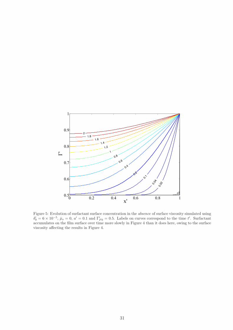
2e−07

0.0

2

0.0

4

0.1

0.2

0.4

0.6

0.8

1

1.2

1.4

1.6

1.8

2

� ��� ��� ��� �� ���

���

���

��

��

Figure 5: Evolution of surfactant surface concentration in the absence of surface viscosity simulated usingδ′0 = 6 × 10−5, µs = 0, a′ = 0.1 and Γ′

F0 = 0.5. Labels on curves correspond to the time t′. Surfactantaccumulates on the film surface over time more slowly in Figure 4 than it does here, owing to the surfaceviscosity affecting the results in Figure 4.

31

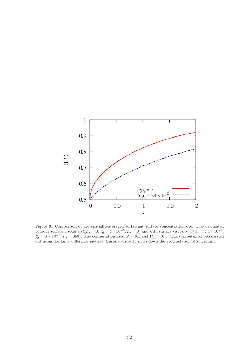
0.5

0.6

0.7

0.8

0.9

1

0 0.5 1 1.5 2

⟨Γ’

⟩

t’

δ’0

-µ

s = 0

δ’0

-µ

s = 5.4 × 10

-2

Figure 6: Comparison of the spatially-averaged surfactant surface concentration over time calculatedwithout surface viscosity (δ′0µs = 0, δ′0 = 6× 10−5, µs = 0) and with surface viscosity (δ′0µs = 5.4× 10−2,δ′0 = 6 × 10−5, µs = 886). The computation used a′ = 0.1 and Γ′

F0 = 0.5. The computation was carriedout using the finite difference method. Surface viscosity slows down the accumulation of surfactant.

32

u'' s

0.4

0.2

2e−06

2

1

4

6

8

10

12

14

16

18

20

0 0.2 0.4 0.6 0.8 1

−0.045

−0.04

−0.035

−0.03

−0.025

−0.02

−0.015

−0.01

−0.005

0

u'' s

0.40.2

2e-06

12

4

6

8

10

12

1416

18 20

0.85 0.9 0.95 1

-0.04

-0.02

0

Figure 7: Evolution of surface velocity calculated using δ′0µs = 5.4 (obtained from δ′0 = 6 × 10−5 andµs = 8.86 × 104), a′ = 0.1 and Γ′

F0 = 0.5. The computation was carried out using the finite differencemethod. Labels on curves are the rescaled dimensionless time t′′. The inset is zoomed in around x′ = 1.The velocity profiles show a linear variation with x′ over much of the domain, but an abrupt deviationfrom linearity near x′ = 1.

33

��

��

0.41

2

4

6

8

10

12

14

16

18

20

� ��� ��� ��� �� ���

���

���

��

��

Figure 8: Evolution of surfactant surface concentration calculated using parameters δ′0µs = 5.4 (obtainedfrom δ′0 = 6 × 10−5 and µs = 8.86 × 104), a′ = 0.1 and Γ′

F0 = 0.5. The computation was carried outusing the finite difference/material point method. Labels on curves are the rescaled dimensionless timet′′. The profiles show a uniform concentration region over much of the domain with an abrupt change inconcentration at the end of the domain.

34

x'

Γ'

2e−06

1

2

4

6

8

10

12

14

16

18

20

0 0.2 0.4 0.6 0.8 10.5

0.6

0.7

0.8

0.9

1

Figure 9: Evolution of surfactant surface concentration calculated with the integro-differential equation(as described in the appendix, and applicable for δ′0µs → ∞), using parameters a′ = 0.1 and Γ′

F0 = 0.5.Labels on curves are the rescaled dimensionless time t′′. Close agreement is seen between the integro-differential equation results here (δ′0µs → ∞) and the finite difference results (Figure 8 with δ′0µs = 5.4).

35

0.5

0.55

0.6

0.65

0.7

0.75

0.8

0.85

0 5 10 15 20

Γ’

t’’

δ0’-µ

s → ∞

δ0’-µ

s = 5.40

δ0’-µ

s = 2.70

δ0’-µ

s = 0.54

Figure 10: Comparison of the spatially-averaged surfactant surface concentration over time calculatedusing the integro-differential equation (δ′0µs → ∞) and the finite difference/material point method (δ′0 =6 × 10−5, µs = 8.86 × 104, δ′0µs = 5.4) with additional data for δ′0µs = 2.7 and 0.54 also includedfor comparison. All computations had a′ = 0.1 and Γ′

F0 = 0.5. Data for δ′0µs → ∞, δ′0µs = 5.4 andδ′0µs = 2.7 are difficult to distinguish on the scale of the plot. Differences start to appear as δ′0µs decreases,e.g. for the case δ′0µs = 0.54.

36

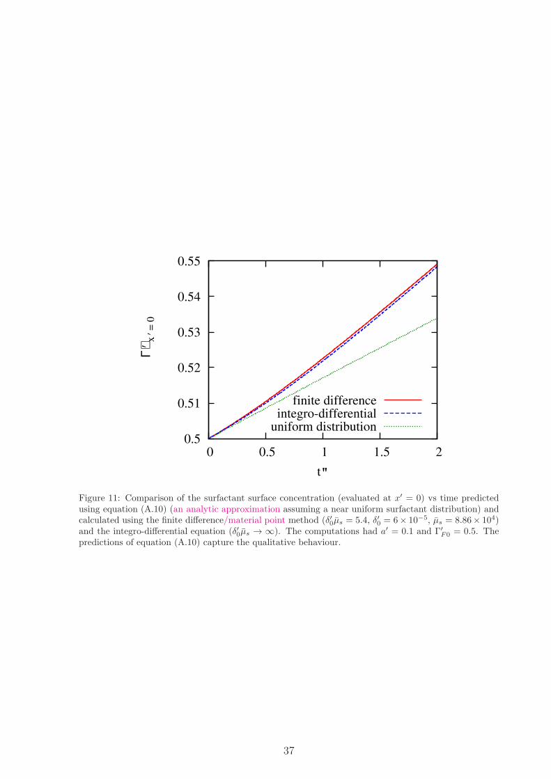
0.5

0.51

0.52

0.53

0.54

0.55

0 0.5 1 1.5 2

Γ’x’

= 0

t"

finite differenceintegro-differential

uniform distribution

Figure 11: Comparison of the surfactant surface concentration (evaluated at x′ = 0) vs time predictedusing equation (A.10) (an analytic approximation assuming a near uniform surfactant distribution) andcalculated using the finite difference/material point method (δ′0µs = 5.4, δ′0 = 6× 10−5, µs = 8.86× 104)and the integro-differential equation (δ′0µs → ∞). The computations had a′ = 0.1 and Γ′

F0 = 0.5. Thepredictions of equation (A.10) capture the qualitative behaviour.

37

0.5

0.6

0.7

0.8

0.9

1

0 0.5 1 1.5 2

⟨Γ’

⟩

t’

δ’0

-µ

s = 0

δ’0

-µ

s = 5.4 × 10

-2

δ’0

-µ

s = 5.4

Figure 12: Comparison of the spatially-averaged surfactant surface concentration over time calculated inthe absence of surface viscosity and in the presence of surface viscosity (δ′0µs = 0–5.4, µs = 0–8.86×104).The simulation used δ′0 = 6 × 10−5, a′ = 0.1 and Γ′

F0 = 0.5. Computations were carried out using thefinite difference/material point method. High surface viscosity severely limits the rate at which surfactantaccumulates on the film.

38

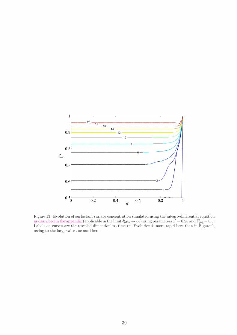
x'

'

2e 06

1

2

4

6

8

10

12

14

1618

20

0 0.2 0.4 0. 0. 10.5

0.

0.

0.

0.9

1

Figure 13: Evolution of surfactant surface concentration simulated using the integro-differential equationas described in the appendix (applicable in the limit δ′0µs → ∞) using parameters a′ = 0.25 and Γ′

F0 = 0.5.Labels on curves are the rescaled dimensionless time t′′. Evolution is more rapid here than in Figure 9,owing to the larger a′ value used here.

39

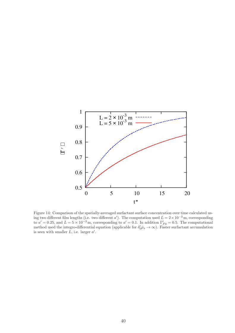
0.5

0.6

0.7

0.8

0.9

1

0 5 10 15 20

⟨Γ’

⟩

t"

L = 2 × 10-3

mL = 5 × 10

-3 m

Figure 14: Comparison of the spatially-averaged surfactant surface concentration over time calculated us-ing two different film lengths (i.e. two different a′). The computation used L = 2×10−3m, correspondingto a′ = 0.25, and L = 5× 10−3m, corresponding to a′ = 0.1. In addition Γ′

F0 = 0.5. The computationalmethod used the integro-differential equation (applicable for δ′0µs → ∞). Faster surfactant accumulationis seen with smaller L, i.e. larger a′.

40