Superstar Extinction

Pierre Azoulay Joshua Graff Zivin Jialan WangMIT and NBER Columbia University and NBER MIT

Sloan School of Management Mailman School of Public Health Sloan School of Management50 Memorial Drive, E52-555 600 West 168th Street, Room 608 50 Memorial Drive, E52-416

Cambridge, MA 02142 New York, NY 10032 Cambridge, MA 02142

December 4, 2007

Abstract

We estimate the magnitude of spillovers generated by 137 academic “superstars” in the lifesciences onto their coauthors’ research productivity. These researchers died while still beingactively engaged in science, thus providing an exogenous source of variation in the structureof their collaborators’ coauthorship networks. Following the death of a superstar, we find thatcoauthors suffer a lasting 8 to 18% decline in their quality-adjusted publication output. Thesefindings are surprisingly homogenous across a wide range of coauthor and coauthor/superstardyad characteristics. Together, they suggest that part of the scientific field embodied in the“invisible college” of coauthors working in that area dies along with the star — that theextinction of a star represents a genuine and irreplaceable loss of human capital.

Keywords: knowledge spillovers, economics of science, collaboration, careers.

∗preliminary and incomplete. Send correspondence to pazoulay@mit.edu. Part of the work was performed while thefirst author was an Alfred P. Sloan Industry Studies Fellow. We gratefully acknowledge the financial support of the Na-tional Science Foundation (Award SBE-0738142) and the Merck Foundation through the Columbia-Stanford Consortium onMedical Innovation. The project would not have been possible without Andrew Stellman’s extraordinary programming skills(http://www.stellman-greene.com/). The authors also express gratitude to the Association of American Medical Colleges forproviding licensed access to the AAMC Faculty Roster. We wish to acknowledge the stewardship of Dr. Hershel Alexander(AAMC Director of Faculty Data Systems and Studies). The National Institutes of Health partially supports the AAMCFaculty Roster under contract N01-OD-3-1015. The usual disclaimer applies.

1 Introduction

Human capital, through its influence on the creation and adoption of improved technologies,

has long been recognized as an important contributor to aggregate income (Nelson and

Phelps, 1965; Schultz, 1967). Modern economic growth models have built upon this idea to

argue that human capital externalities — knowledge spillovers across individuals — are the

principal drivers of economic progress (Lucas, 1988; Romer, 1990). The skills and wisdom of

some individuals, through interactions with others, increases these attributes in their peers.

The increased stock of human capital in the economy generates more ideas and faster growth.

The empirical literature on human capital externalities is relatively small and principally

focused on the estimation of peer effects among students (e.g., Rauch, 1993; Acemoglu

and Angrist, 2001; Hoxby, 2000; Sacerdote, 2001). Yet, the endogenous growth literature

typically envisions spillovers that occur in the workplace, where firms acquire ideas from their

neighbors and employees learn from their co-workers. Indeed, the importance of learning

through social interactions on the job can be traced back to turn of the century writings by

Alfred Marshall (1890). Only a handful of empirical papers have examined peer effects in

the employment setting.1

The paucity of literature is largely due to the difficulties involved in collecting the data

necessary to measure these effects. In most employment settings, it is often impossible to

identify peer groups at the individual level, and even harder to distinguish output produced

jointly with the peer group from output produced independently of it. As a result, the

existing research often relies on aggregate proxies — such as co-location — to estimate human

capital externalities. Moretti (2004) exemplifies this approach. Using the share of college

graduates in the workforce at the city level, he provides evidence for modest human capital

externalities in the US manufacturing sector and also finds that spillovers are larger among

1A related literature examines the influence of peer effects on shirking behavior in the workplace (Ichinoand Maggi, 2000; Costa and Khan, 2003; Bandiera et al., 2005; Mas and Moretti, 2006). Since shirking iseasily observed by co-workers and “contagion” does not generally involve the transmission of knowledge ortechniques, this type of spillover is conceptually distinct from human capital externalities.

1

firms that are economically similar. Since manufacturing is less human capital intensive than

other sectors of the economy, the finding that spillovers are modest is perhaps not surprising.

In this paper, we attempt to relax the data constraint by focusing on a setting where hu-

man capital externalities are likely to be quite important — the academic life sciences.2 This

choice enables us to estimate the productivity benefits of knowledge spillovers at the individ-

ual level. It also allows us to trace these spillovers back to social interactions, independently

of location decisions. The importance of social interactions is supported by recent evidence

from Kim et al. (2006) who show that spillovers, at least among academic economists, have

become less tied to physical location over time, perhaps due to improvements in information

technologies. Moreover, our focus on connections between individuals of differing skill levels

speaks directly to the types of human capital externalities envisaged by the early champions

of modern economic growth theory, as exemplified by the following quote from Lucas (1988):

“Most of what we know we learn from other people. We pay tuition to a few of theseteachers, either directly or indirectly by accepting lower pay so we can hang aroundthem, but most of it we get for free, and often in ways that are mutual — without adistinction between student and teacher. Certainly in our own profession, the benefitsfrom colleagues from whom we hope to learn are tangible enough to lead us to spend aconsiderable fraction of our time fighting over who they shall be, and another fractiontraveling to talk with those we wish we could have as colleagues but cannot. We knowthat this kind of external effect is common to all the arts and sciences — the ‘creativeprofessions.’ All intellectual history is the history of such effects.”

More specifically, we analyze the research productivity of coauthors for 137 eminent life

scientists who die prematurely, while still being actively engaged in science. These scientists

are drawn from a larger sample of superstar academics selected on the basis seven different

criteria, including NIH funding, citations, patents, membership in the National Academy

of Sciences, or appointment as Howard Hughes Medical Investigator. Using a matched

faculty-university panel dataset, we measure how colleagues’ scientific output, as measured

by quality-adjusted publications, changes when their superstar collaborator passes away. To

2Weinberg (2007) pursues a similar strategy, focusing on physicists, and analyzing how geographic prox-imity to earlier Nobelists correlates with the start of the research that would eventually result in a NobelPrize.

2

be clear, our focus is on faculty peers, not trainees, and thus our results should be viewed

as capturing inter-laboratory spillovers rather than mentorship effects.

Economists have long recognized the difficulties involved in recovering causal effects in

observational studies of peer influence (e.g., Manski 1993). Certainly, the formation of col-

laborative relationships should be understood as outcomes of a purposeful matching process

(Fafchamps et al., 2006; Mairesse and Turner, 2005). Therefore, our approach is to condition

inclusion in the sample on a coauthorship tie, and to focus instead on the deletion of this

tie induced by the death of a prominent collaborator. Because we can identify 73 coauthors

per superstar on average, we can exploit rich variation in the depth and length of interaction

to examine potential heterogeneity in the treatment effect. Other economists have used the

death of prominent individuals as a source of exogenous variation in leadership, whether in

the context of business firms (Johnson et al., 1985; Bennedsen et al., 2007), or even entire

countries (Jones and Olken, 2005). To our knowledge, however, we are the first to use this

strategy to estimate the magnitude of knowledge spillovers.

Our results reveal an 8 to 18% decrease in the quality-adjusted publication output of

coauthors in response to the sudden and unexpected loss of a superstar. When the superstar

death is anticipated and thus less plausibly exogenous, our results are weaker but gener-

ally consistent with the effects due to unanticipated losses. More interestingly, the impact

of star death is quite diffuse — output declines are similar irrespective of geographic dis-

tance between collaborators, the time since last collaboration, or whether the coauthor was

formerly a trainee of the star. We also verify that the effects we measure are increasing

in the superstar’s intellectual accomplishments (measured by citation count at the time of

death) and not their financial ones (measured by NIH grantsmanship at the time of death).

This suggests that spillovers are indeed about knowledge and that the loss of a coauthor of

lesser rank would not generate the long lasting effects of the type we find here. The only

researchers that appear insulated from these negative effects of star death are those who are

themselves among the highest achievers in their field, as measured by membership in the

National Academy of Sciences, and those who are significantly more senior than the star.

Together, these results paint a picture of an invisible college of coauthors bound together

3

by interests in a fairly narrow scientific area, which suffers a permanent and reverberating

intellectual loss when it loses its star.

The rest of the paper proceeds as follows. In the next section, we provide a brief theoret-

ical background for the study. Section 3 presents our sample of superstars and describes the

matching process necessary for the identification of colleagues. Section 4 presents descriptive

statistics, and reports econometric results. Section 5 concludes.

2 Theoretical Background

Knowledge can flow across time and space through three distinct mechanisms. The endoge-

nous growth literature emphasizes the “standing on shoulders of giants” effect, whereby the

current state of knowledge forms the basis for new knowledge-based innovation. This im-

plies a role for education and training, which enable would-be innovators to be active at

the frontier of knowledge (Jones, 2005). A second mechanism for knowledge diffusion is

involuntary spillovers, whereby innovators obtain knowledge generated by others through

observation and imitation. Finally, knowledge can be shared directly among members of

innovating teams. Here we envision an “invisible college”, where strong intellectual ties can

create an informational network in which the main ideas of a new field are created (Crane,

1972). In this paper, we are interested in evaluating the extent to which such collaborations

can foster the production of new knowledge.

Looking at the effect of collaborations is important because very few innovations result

from the efforts of lone researchers engaged in otherworldly contemplation. The creative

process is characterized by the search for useful recombinations of existing ideas (Weitzman,

1998), and the mixing of individuals with different backgrounds and education within the

same team magnifies the number of combinations that can be evaluated. Moreover, members

of these teams do not have to be colocated. In fact, they are increasingly distributed across

4

different locales, thanks to the use of information and communication technologies (Kim et

al., 2006; Rosenblat and Mobius, 2004).3

When members of different skill level or experience match, less skilled agents might

gain from their exposure to the ideas of the relatively more skilled, thus creating voluntary

spillovers of knowledge. A skilled agent might match with a less skilled one by pure al-

truism, because of cultural norms that favor professional mentorship, or because the costs

of collaboration with less-skilled agents are lower. Here, we will take the existence of such

heterogeneous matches as given, and exploit the exogenous termination of these relations

induced by death to study their impact on the output produced by the relatively less skilled.

The impact of the skilled on the less skilled is especially interesting because the former

might find it difficult to fully appropriate the benefits they confer on the latter. For ex-

ample, it might be impossible to apportion credit between team members in ways that are

verifiable by a court. Moreover, even when individual talent is perfectly observed in the

market, asymmetric information over the mentorship abilities of skilled agents might both

limit their mobility and ensure that they cannot extract their full marginal product (Lazear,

1986; Acemoglu and Pischke, 1999).

That knowledge spillovers are at least partially external means innovators will have too

little incentive to innovate (Murphy et al., 1991). In such a world, the allocation of talent

across firms and the technologies and policies that influence the flow of information between

agents has important implications for the level and rate of technological innovation within

the economy, and eventually for economic growth.

The setting chosen for our empirical work is the academic life sciences. This sector

is an important one to study for several reasons. First, technological change has been

enormously important in the growth of the health care economy, which accounts for roughly

15% of US GDP. Much biomedical innovation is science-based (Henderson et al., 1999),

and interactions between academic researchers and their counterparts in industry appear

3In a related vein, Agrawal and Goldfarb (2006) provide persuasive evidence that the diffusion of BITNET,an early precursor to the internet, fostered collaboration between computer scientists in first- and second-tierresearch universities.

5

to be an important determinant of research productivity in the pharmaceutical industry

(Cockburn and Henderson, 1998; Zucker et al., 1998; Powell et al., 2005). Second, and

perhaps most importantly for our work, academic scientists are generally paid through soft

money contracts. Salaries depend on the amount of grant revenue raised by faculty, thus

providing researchers with high-powered incentives to remain productive even after they

secure a tenured position. As such, academic life scientists can be viewed as entrepreneurs

producing new knowledge through the management of small idiosyncratic firms, comprised

of junior faculty, postdoctoral researchers, graduate students, and other research personnel.

Lastly, there are large public subsidies for biomedical research in the United States. With

an annual budget of $28 billion in 2004, support for the NIH dwarfs that of other national

funding agencies in developed countries (Cech, 2005). Thus, estimating knowledge spillovers

in this sector will allow us to better assess the return to these public investments.

Our focus on this setting — one with a very extensive paper trail of research output and

collaboration histories — also offers practical benefits that better enable us to examine the

magnitude of human capital externalities. By matching data on quality-adjusted publication

output with an administrative dataset linking medical school scientists with their employers,

we are able to create what is, to our knowledge, the first matched employee-employer dataset

with individual-level measures of output.

The rich coauthorship tradition in the life sciences also allows us to identify peer groups

more precisely than the standard approach in the literature, which uses colocation as a

de facto measure of social interaction (Jaffe et al., 1993). While attending to geographic

distance, we use collaborations between scientists to define actual interactions, thus draw-

ing boundaries around the ethereal invisible college. Collaborations are important because

research areas in the biomedical sciences are highly specialized and the set of individuals

writing together on this subject is a better measure of the scientific field than school, de-

partment, or even discipline. To fix ideas, spheres of influence, and thus fields of inquiry,

are not defined in broad categories such as genetics, but rather around ideas related to the

regulation of vascular endothelial growth factor during nerve regeneration, perhaps only in

mice and rats. As discussed earlier, we overcome concerns about the endogeneity of these

6

relations, by focusing on the impacts induced by the exogenous termination of collaborations

due to the death of a superstar.

3 Data and Sample Characteristics

This section provides a detailed description of the process through which the matched coau-

thor/superstar data used in the econometric analysis was assembled. In order, we describe (1)

the criteria used to select our sample of superstar life scientists; (2) the universe of potential

colleagues for these superstars; and (3) the essence of the matching procedure implemented

to identify actual colleagues from coauthorship records. We also present basic demographic

characteristics for the superstars, as well as descriptive statistics for the individual coauthors

and superstar/coauthor dyads.

3.1 Superstar Sample

Our basic approach is to rely on the death of “superstar” scientists to estimate the magnitude

of knowledge spillovers onto colleagues. In particular, we limit our attention to those stars

that were still active researchers when they died prematurely at an age less than or equal

to 66 years. Our focus on superstars can be justified on both substantive and pragmatic

grounds. Significant inequality in scientists’ productivity has been widely documented. In

a classic paper, Lotka (1926) showed that the most productive 6% of publishing physicists

produced 50% of the papers in the journals he examined. An extensive literature in the

sociology of science presents further evidence of the skewed distribution of productivity

(e.g., Merton, 1973; de Solla Price, 1986). In a related vein, Zucker et al. (1998) established

a robust correlation between the location of superstar life scientists and the number of new

biotechnology firms spawned in a given locale. Thus, if one wants to find evidence of spillovers

at the individual level, it seems logical to start with a sample of superstars, rather than with

a random sample of scientists. From a practical standpoint, it is more feasible — though

still surprisingly difficult — to trace back the careers of eminent scientists than to perform a

similar exercise for less eminent ones. As we will see in Section 4, our motivation for focusing

7

on stars is also supported by our empirical work, which shows that the impact of star death

is increasing in his/her accomplishments. The subset of stars used in our analysis is drawn

from a larger pool of 7,276 eminent life scientists who are so classified if they satisfy at least

one of the following seven criteria for scientific achievement.

• Highly Funded Scientists. Our first source is the Consolidated Grant/Applicant

File (CGAF) from the U.S. National Institutes of Health (NIH). This dataset records

information about grants awarded to extramural researchers funded by the NIH since

1938. Using the CGAF, and focusing only on research grants, we compute individual

cumulative totals for the years 1977 to 2003, deflating the earlier years by the biomed-

ical research producer price index. We also recompute these totals excluding large

center grants that usually fund groups of investigators (M01 and P01 grants). Those

scientists whose totals lie in the top ventile (i.e., above the 95th percentile) of either of

these two distributions constitute our first group of superstars. In this elite group, the

least well-funded investigator had garnered $10.5 million in NIH career funding, and

the most well-funded $462.6 million.

• MERIT Awardees of the NIH. In order to include a more explicitly quality-focused

measure of grantsmanship, we also include MERIT awardees from the NIH. Initiated

in the mid-1980s, the MERIT (Method to Extend Research in Time) Award pro-

gram extends funding to experienced investigators with impressive records of scientific

achievement in research areas of special importance or promise. Investigators cannot

apply for a MERIT award and less than 1% of NIH-funded researchers are selected to

receive them.

• Highly Cited Scientists. Despite the preeminent role of the NIH in the funding of

public biomedical research, this indicator of “superstardom” biases the sample towards

older scientists conducting relatively expensive research. We complement this first

group with a second composed of highly cited scientists identified by the Institute for

Scientific Information. A Highly Cited listing means that an individual was among the

8

250 most cited researchers for their published articles between 1981 and 1999, within

a broad scientific field.4

• Howard Hughes Medical Investigators. We also drew on the population of cur-

rent or former Howard Hughes Medical Investigators. Every three years, the Howard

Hughes Medical Institute solicits nominations from research institution, with the aim of

identifying researchers who have the potential to make significant contributions to sci-

ence. Once selected, they continue to be based at their institutions, typically leading a

research group of 10 to 25 students, postdoctoral associates and technicians. From our

point of view, HHMIs are attractive in that they tend to be younger, “up-and-coming”

scientists, rather than established investigators.

• Pew and Searle Scholars. We also included Pew and Searle scholars for the years

1981 through 2000. Every year, the Pew and Searle charitable trusts provide seed

funding to 40 life scientists in the first two years of their careers as independent in-

vestigators. The Pew and Searle Scholarships are the most prestigious accolades that

young researchers can receive at the start of their careers.

• Top Patenters. We add to these groups academic life scientists who belong in the

top percentile of the patent distribution among academics — those who were granted

17 patents or more between 1976 and 2004.

• National Academy of Sciences. Finally, we add to these groups academic life

scientists who were elected to the National Academy of Science between 1975 and

2007.

Tables 1A and 1B present individual-level details on the superstar sample, broken down

by sudden and anticipated deaths, respectively. Heart attack is the most frequent cause of

sudden death, while the vast majority of anticipated deaths are due to some form of cancer.

Since most of the anticipated deaths are due to conditions with short life expectancies and

4The relevant scientific fields in the life sciences are microbiology; biochemistry; psychiatry/psychology;neuroscience; molecular biology & genetics; immunology; pharmacology; and clinical medicine.

9

those with longer ones are not necessarily viewed as terminal until the final stages, anticipated

deaths should be thought of as those with no more than several years notice.

Many scientists achieve superstar status according to more than one metric. We trace

back these scientists’ careers with great care from the time they obtain their first position

as independent investigators (typically after a postdoctoral fellowship) until 2006. We do so

through Who’s Who profiles, accolades/obituaries in medical journals, National Academy

of Sciences biographical memoirs, and Google searches. As a result, we are able to trace

back their path from humble beginnings to superstardom, and to examine whether spillovers

vary over the life cycle, even though selection into the sample was based on cumulative

achievement.

We record employment history, degree held, date of degree, gender, up to three depart-

ments, and whether the star held an administrative position, such as dean or hospital CEO.

We cross-reference the superstar sample with other measures of scientific eminence. For

example, our 137 superstars include one Nobel Prize winner and two Lasker awardees.

Table 2A provides descriptive statistics for the superstar sample. The average star re-

ceived their degree in 1965, died at 58 years old, held 1.75 positions in their career, and

worked with 73 coauthors in their lifetime. The youngest died at 35 and the oldest died at

66. The most gregarious worked with 225 coauthors over the course of their career. On the

output side, the stars each received an average of roughly 22 million dollars in NIH grants,

published 161 papers, garnered 10,240 citations, and held 2 patents. We also compute the

h index due to Hirsch (2005), which is commonly used by bibliometricians: h is the highest

integer such that an individual has h publications cited at least h times. In our sample, h

is approximately 50. The most well-funded investigator received 203 million dollars in NIH

funding and the most prolific wrote 533 papers. The subsample of superstars whose death

was anticipated appears slightly more accomplished on average, but not dramatically so.

Table 2B provides additional information about the superstar sample. The sample is

approximately 12% female and 84% US-born. 42% of our stars hold an MD degree, 47% a

PhD, and the remainder hold dual MD/PhD degrees. Keeping in mind that our metrics of

10

superstardom are not mutually exclusive, roughly 7.3% are Howard Hughes Medical Inves-

tigators, 34.3% are MERIT awardees, and 21.9% are members of the National Academy of

Sciences.

3.2 The Universe of Potential Colleagues

Information about superstars’ colleagues stems from the Faculty Roster of the Association of

American Medical Colleges, whose access we secured for the years 1977 through 2006 under

a licensing agreement. The roster is an annual census of all U.S. medical school faculty,

where each faculty is linked across yearly cross-sections by a unique identifier.5 When all

cross-sections are pooled, we obtain a matched employee/employer panel dataset. For each

of the 222,478 faculty members that appear in the roster, we know the full name, the type

of degrees received and the years they were awarded, gender, up to two departments, and

medical school affiliation. Besides its comprehensiveness, an attractive feature of this data

source is that it shares a common system of individual identifiers with the CGAF dataset.

Because the roster only lists medical school faculty, however, it is not a complete census of

the academic life sciences. For instance, it does not list information for faculty at institutions

such as MIT, University of California at Berkeley, Rockefeller University, the Salk Institute,

or the Bethesda campus of the NIH; and it also ignores faculty members in Arts and Sciences

departments — such as biology and chemistry — if they do not hold joint appointments at

a local medical school.6

For the purposes of this paper, we define colleagues to be those faculty listed on the

roster that are coauthors for each superstar. While this is certainly not the only basis

5Although AAMC does not collect data from each medical school with a fixed due date. Instead, itcollects data on a rolling basis, with each medical school submitting on a time frame that best meets itsreporting needs. Nearly all medical schools report once a year, while many medical schools update oncesemester. Other medical schools update once a month or even more often than that if the medical schoolsuse the Faculty Roster as their primary database for maintaining faculty data.

6This limitation is less important than might appear at first glance. First, we have no reason to thinkthat colleagues located in these institutions differ in substantive ways from those based in medical schools.Second, all our analyses focus on changes in research productivity over time for a given scientist. Therefore,the limited coverage is an issue solely for the small number of faculty who transition in and out of medicalschools from (or to) other types of research employment. For these faculty, we were quite successful in fillingout career gaps by combining the roster with the NIH data.

11

upon which colleagues could be defined, a coauthorship-based definition seems the most

sensible.7 The production of abstract knowledge depends on the extent to which ideas

are shared among researchers, and an important mechanism for sharing knowledge is direct

collaboration through coauthorship. Moreover, the coauthorship network is our best measure

of scientific field in a universe with researchers who are highly specialized. It bears repeating

that the typical social scientist’s broad conceptualization of field is somewhat misguided

here. A physiologist working on protein trafficking between intracellular organelles will

not necessarily be influenced by developments in physiology writ large, but certainly follow

closely the research of those working in his/her narrow area of inquiry. Indeed, the sphere

of influence may even be limited to those engaged in research on protein trafficking for the

Moloney murine leukemia virus.

3.3 Coauthor Matching

To identify coauthors, we have developed a custom software program, the Stars/Colleagues

Generator, or S/CGen.8 The source of the publication data is PubMed, an online resource

from the National Library of Medicine that provides fast, free, and reliable access to the

biomedical research literature. In a first step, the S/CGen downloads from the internet the

7Specifically, we could have labeled colleagues any faculty that was co-located with the superstar at anypoint during his or her career. This does not strike us as a meaningful definition of the term “peer,” becausemedical schools are large research institutions (833 faculty on average in 2003). One could make use ofdepartment information to define narrower boundaries for peer groups, but this approach is too difficultto implement in practice. First, department affiliations are not fixed over time for most faculty — this isapparent in our sample of superstars, and many collaborations span departmental boundaries. Second, newdepartments were created during this period (e.g., Neuroscience, Genetics, or Biomedical Engineering), whileothers were phased out or dramatically shrunk (e.g., Anatomy). Third, the merging or survival of manydepartments is often a reflection of internal political struggles, rather than characteristics of the researchconducted within them. For example, in some medical schools, orthopedic surgeons are in a separate de-partment while in others, they are part of a large surgery department; In the basic sciences, many facultywould feel equally at home in cell biology, molecular biology, or biochemistry. Finally, three large depart-ments (internal medicine, pediatrics, and surgery) tend to account for a large proportion of medical schoolemployment, but their size masks enormous heterogeneity (e.g., neurosurgeons vs. cardio-thoracic surgeons;endocrinologists vs. infectious diseases specialists).

8The complete specifications are described in a technical working paper (Stellman et al., 2006), while theS/CGen software itself can be used by other researchers under a GNU license. Note that the S/CGen takesthe faculty roster as an input; we are not authorized to share this data with third-parties. However, it canbe licensed (for a fee) from AAMC, provided a local IRB gives its approval and a confidentiality agreementprotects the anonymity of individual faculty members.

12

entire set of English-language articles for a superstar, provided they are not letters to the

editor, comments, or other “atypical” articles. From this set of publications, the S/CGen

strips out the list of coauthors, eliminates duplicate names, matches each coauthor with

the Faculty Roster, and stores the identifier of every coauthor for whom a match is found.

In a final step, the software queries PubMed for each validated coauthor, and generates

publication counts as well as coauthorship variables for each superstar/colleague dyad, in

each year.

S/CGen cannot generate a match for each coauthor. Some coauthors are postdocs,

technicians, or graduate students who do not go on to faculty positions within our period of

observation; other coauthors have positions in foreign institutions; others still publish under

names that differ from the faculty roster listing (for instance by being inconsistent with the

use of middle initials, suffixes, or hyphens). We are more worried about generating spurious

matches, however.

An important limitation in the matching process is that PubMed does not record authors’

full names, nor does it record their institutional affiliation; it only keeps track of authors by

using a combination of last name, two initials, and a suffix (where the suffix and the second

initial fields can be empty). There are no unique author identifiers, and no possibility to

account for the different name variations that a given author uses throughout his/her career.

This absence of unique author identifiers could create a cascade of errors. For a superstar

with a relatively common name (e.g., Thomas W. Smith), a simple query would return many

publications that were, in fact, not his. As a consequence, a number of coauthors identified

by our software would be spurious. This source of error would be compounded by the fact

that when searching for the colleagues’ publications, the output of those with relatively

more frequent names will be imprecisely measured. The first source of error strikes us as

potentially very serious, and to deal with it, we designed custom search queries that return

a superstar’s list of publications excluding those of any homonymous scientist.9

9These queries form part of the information that the software takes as an input. They can be up to 244characters long (see Stellman et al. (2006) for more details).

13

After neutralizing this first source of error, it is still the case that S/CGen can generate

more than one roster match for a given PubMed author name, and the quality of these

matches will depend directly on the relative frequency of last names in the population.

In order to ensure that publications are assigned to authors as precisely as possible, the

analysis that follows is based only on those colleagues with unique PubMed names, i.e.,

those combinations of last names, two initials, and suffix which correspond to one, and only

one, faculty member in the roster.10

3.4 Control Coauthors

Our original research design calls can identify changes in output trends for coauthors after a

superstar coauthor passes away, relative to before. With a single level of difference, we rely

on the coauthors of stars who have not died yet as an implicit control group to pin down

life cycle and calendar time effects. This will provide estimates that can be given a causal

interpretation under fairly general assumptions regarding the exogeneity of the death event.

However, the before/after contrast might be misleading if collaborations with superstars are

subject to idiosyncratic dynamic patterns. For example, collaborations might grow stale over

time, and our estimates might (in part) reflect this natural evolution rather than spillovers.

Alternatively, happenstance might yield a sample of stars clustered in decaying scientific

fields. Therefore, we adduce to the data a set of control coauthors so that we can analyze the

impact of superstar death in a difference-in-differences set-up. In creating a suitable control

group, we face two hurdles. First, we only have a small set of observable characteristics

available to match coauthors. Second, the death of one of our 137 superstars should have no

effect on the output of a suitable control coauthor. This is problematic because of indirect

coauthorship ties: it is almost impossible to find scientists that are isolates in the network

formed by life scientists and their collaborations.

Because of the first issue, we begin by finding controls for the 137 superstars who die

among our set of 7,276 eminent scientists. We first eliminate from the set of potential controls

10To fix ideas, Lechleiter JD is an example of unique PubMed name. In contrast, Weinstein SL corre-sponds to two distinct faculty in the roster, Miller MJ to ten, and Wang Y to thirty six.

14

any scientist who coauthored with one of the treated superstar. We then run a logit, using

a large number of covariates: publications, citations, funding, patents, number of coauthors,

degree, gender, department, age, etc., to predict death in the set of 3,444 scientists who

remain after applying this screen. Our favored specification has a pseudo-R2 of .173, and we

use the predicted value to select two “nearest neighbor” superstars for each of the superstars

who dies. In other words, we identify 232 eminent scientists who appear similar (based

on observable characteristics) to the 137 superstars that are the focus of the paper. The

coauthors of those 232 superstars constitute our control group. Of course, it is sometimes

the case that scientists who coauthor with the 232 control superstars also coauthor with one

or more of the 137 focal superstars. In every specification that makes use of the controls,

we eliminate from the estimation sample these “problematic” coauthors. This implies that

the minimum path length between a control coauthor and a treated coauthor is 3 when

we constrain the paths to pass through at least one of our 7,276 superstars. As a result,

we are quite confident that our control sample is relatively “uncontaminated” by indirect

coauthorship ties. Figure 1 presents a stylized schema of the coauthorship ties between

control and treatment coauthors that are allowed by our data assembly process, and contrast

them with the ties that we rule out.11

3.5 Descriptive Statistics

When applied to our sample of 232+137 = 369 superstars, S/CGen software identifies 15,715

scientists with unique PubMed names (11,033 controls and 4,682 treated coauthors). This

translates into approximately 73 coauthors per superstar on average (the median is 68) —

the distribution for the 137 superstars that die is displayed in Figure 2. Approximately 46%

of all coauthors are MDs, 45% are PhDs, and the remainder are joint degree holders (see

Table 3). It is appropriate to describe the data at two different levels, that of the individual

11Nothing precludes one of the 7,276 eminent scientists to play the role of coauthor in some dyads (as is thecase for Europa, Orion’s coauthor in Figure 1). In fact, such “star/star” dyads correspond to approximately20% of the data. This reflects the importance of assortative matching in determining the structure ofcollaboration networks.

15

peer, and that of the superstar/coauthor dyad. The software generates 7,392 treatment

dyads, for a total of 191,046 dyad-year observations between 1975 and 2006.

Colleague characteristics. The demographic characteristics for the coauthors are pre-

sented in Table 5. Approximately two-thirds are affiliated with a clinical, rather than basic

science, department. Nearly half hold an MD degree and 19% of them are female. In terms of

research productivity, they lag behind their superstar counterparts, but the difference is not

dramatic (99 vs. 161, on average). This can be explained in two ways. First, these eminent

academics’ careers were cut short, and as a result, they have had less time to accumulate

publications. Second, assortative matching implies that many of their coauthors will also be

eminent scientists. The average coauthor has approximately 99 career publications, $5 mil-

lion in career NIH funding, and one patent. Approximately 88.2% of colleagues publish with

only one of our 369 superstar in their careers, with the remainder predominantly publishing

with two superstars. Only 53 colleagues coauthor with 4 or more of our superstars in their

career (see Table 4). Note that treated and control coauthors are not perfectly balanced on

observables. The latter are more likely to be female, slightly less likely to receive NIH fund-

ing, and publish 5 papers less on average over their entire career. This lack of perfect balance

is not surprising given the fact that the fit of the logit predicting death among superstars

(on the basis of which the control coauthors were selected) is relatively low.

Dyad characteristics. Here we find it useful to distinguish between coauthors that have

published papers with stars that died suddenly from those who collaborated with stars whose

death was anticipated. Table 6 presents summary statistics for both groups, both of whom

display strikingly similar levels of output. About 23% of the coauthors were closely located

to their superstar coauthors at their time of death, whereas approximately 8% are former

trainees of the star. The descriptive statistics also reveal that these coauthors are far from a

random sample of scientists, as more than half were independently funded by the NIH at the

time of their superstar coauthor’s death. Finally, the distribution of coauthorship intensity

is extremely skewed. As such, we define “casual” coauthors as those that have two or less

coauthorships with the star, “regular” coauthors as those with three to ten coauthorships,

16

and “close” coauthors as those with ten or more coauthorships. Using these definitions,

“regular” dyads correspond to those between the 75th and the 95th percentile of the dyad-

level coauthorship distribution and “close” coauthors correspond to those above the 95th

percentile (displayed in Figure 3).

3.6 Econometric Modeling

Our estimating equation relates peer j’s output in year t to characteristics of i and j:

E [yjt|Xijt] = exp [β0 + β1AFTER DEATHit + f(AGEjt) + δt + γij] (1)

where y is a measure of publication output, AFTER DEATH denotes an indicator variable

that switches to one the year after the superstar dies, f(AGEit) corresponds to a flexible

function of the colleague’s career age, the δt’s stand for a full set of calendar year indicator

variables, and the γij’s correspond to dyad fixed effects, consistent with our approach to

analyze changes in j’s output following the passing of superstar i.

The dyad fixed effects control for many individual characteristics that could influence

research output, such as gender, degree, and scientific field (although changes in department

affiliations are quite frequent). Academic incentives depend on the career stage; given the

shallow slope of post-tenure salary increases, Levin and Stephan (1991) suggest that levels

of investment in research should vary over the career life cycle. To flexibly account for

life cycle effects, we include seven indicator variables corresponding to different career age

brackets, where career age measures the number of years since a scientist earned his/her

highest doctoral degree (MD or PhD).12

Econometric considerations. The number of articles published, patents applied for, or

NIH grants awarded are examples of count dependent variables — non-negative integers

with many zeros and ones. For example, 20.22% of the dyad/year observations in the data

correspond to years of no publication output; the figure climbs to 85.46% if one focuses on

12The omitted category corresponds to faculty members in the very early years of their careers (age 0 to4). It is not possible to separately identify calendar year effects from age effects in the “within” dimensionof a panel in a completely flexible fashion, because one cannot observe two individuals at the same point intime that have the same (career) age but earned their degrees in different years (Hall et al., 2005).

17

the count of successful grant applications, and to 96.92% for the count of patent applications

that eventually issue. Following a long-standing tradition in the study of scientific and tech-

nical change, we present conditional maximum likelihood estimates of eqn. [1] based on the

fixed-effect Poisson model developed by Hausman et al. (1984). Because the Poisson model

is in the linear exponential family, the coefficient estimates remain consistent as long as the

mean of the dependent variable is correctly specified (Gourieroux et al., 1984). Further,

“robust” standard errors are consistent even if the underlying data generating process is not

Poisson. In fact the Hausman et al. estimator can be used for any non-negative depen-

dent variables, whether integer or continuous (Wooldridge, 1997; Santos Silva and Tenreyro,

2006), as long as the variance/covariance matrix is computed using the outer product of

the gradient vector.13 We make our inference conservative by clustering all standard errors

around superstar scientists.

Quality adjustment. To adjust publications for quality, we make use of the Journal

Citation Reports, published yearly by the Institute for Scientific Information. ISI ranks

journals by impact factor (JIF) in different scientific fields. The impact factor is a measure

of the frequency with which the “average article” in a journal has been cited in a particular

year. We weight each article published by the scientists in our sample by the corresponding

journal’s JIF, and compute quality-weighted publication counts in this way.14

Competing stories. Of course, the death of a superstar colleague can influence the pro-

ductivity of their colleagues through channels other than knowledge spillovers. Coauthors

may go through a period of bereavement or even question their commitments to work af-

ter losing a prominent coauthor. Alternatively, the death of a star may represent a loss of

social connections rather than one directly related to knowledge. For example, stars may

13In other words, inference on the coefficient estimates presented below do not make use of the Poissonvariance assumption. We assume only that the conditional mean of our dependent variables can be writ-ten E[y|X] = exp(Xβ), a requirement we consider fairly innocuous, given the non-negative nature of theoutcomes considered here.

14Basically a ratio between citations and recent citable items published, JIFs suffer from built-in biases:they tend to discount the advantage of large journals over small ones, of frequently-issued journals over lessfrequently-issued ones, and of older journals over newer ones. Nonetheless, they convey quite effectively theidea that the New England Journal of Medicine (Impact Factor = 23.223 in 1991) is a much more influentialpublication than the Journal of General Internal Medicine (Impact Factor = 1.056 in 1991).

18

have whispered in the ears of Deans and Project Officers to advocate on the behalf of their

coauthors. Absent the star, these researchers may find it increasingly difficult to access the

financial resources that enable them to conduct research. These competing hypotheses re-

garding the effects of superstar death imply a distinct signature of effects across different

types of colleagues. In the case of bereavement, for example, we would expect the effects

of star death to be immediate and more pronounced among closer colleagues. For internal

social connections, co-located peers should experience larger effects, while impacts related to

external connections should be more pronounced for those working with superstars that are

more centrally located in the coauthorship network. In order to rule out these alternative

explanations (or at least rule them out as the dominant phenomenon underlying our mea-

sured effects) we examine heterogeneity in the response to a break in exposure to superstar

talent more closely. In particular, we interact the treatment effect with various fixed charac-

teristics of the superstar, the colleague, or the dyad at the time the superstar passes away.

These characteristics include geographic proximity, career stage, former trainee status, etc.

Such interactions identify how various coauthor subgroups are differentially impacted by the

death. These differential impacts directly inform our interpretation of the results, i.e., they

can help us distinguish between distinct mechanisms.

4 Results

We begin by validating our contention that our sample of superstars is composed of sci-

entists still actively engaged in science at the time of their death. In Table 7, we present

results for specifications in which the quality-adjusted publication output of our superstars

is regressed on a series of indicator variables corresponding to the timing of death: 4 years

before the year of death, 3 years before the year of death, and so on, up until two years after

the year of death (a scientist can, and often does, publish after his death because his/her

coauthors will typically push articles through the pipeline on his behalf). We stack the deck

in favor of finding preexisting trends in the data by using solely the publications in which

the star appears as last author (last author status is invariably reserved to the head of a

19

laboratory/research group in the life sciences). All models include superstar scientist fixed

effects, and we use as a control group the set of control superstars described above. The

inclusion of controls is important insofar as it enables us to pin down the effect of age and

calendar time, which might be correlated with the death effect.

All estimates are presented in the form of incidence rate ratios; the formula (eβ−1)×100%

(where β denotes an estimated coefficient) provides a number directly interpretable in terms

of elasticity. Model (1), for instance, implies that output falls 1 − 0.61 = 39% in the year

following the year during which the superstar passed away. Column (1) uses all the data, and

uncovers no evidence of decline in output prior to the superstar’s death. In column (2), we

drop the 80 colleagues whose death was anticipated, and obtain similar results. Conversely,

column (3) excludes 57 superstars whose death was sudden and unexpected. The indicator

variables are therefore identified solely off the superstars whose death was anticipated. In

this case, we find modest evidence that scientists who died exhibited higher output in the

year immediately preceding their death. This effect is only significant at the 10% level.

In light of these results, we feel confident that our scientists were still actively engaged in

science at the time of their deaths.

Table 8 presents our core results. The first two columns in Panel A examine the output of

our superstars’ coauthors, regardless of cause of death. We find a sizable and significant 7%

decrease in the total number of quality-adjusted publications they produce after the star dies.

The following two columns concentrate on the coauthors of stars that died suddenly. Here,

we find rather similar results overall — roughly a 10% decrease in total publications, with

a slightly larger effect for regular collaborators. When we turn our attention to anticipated

deaths (columns 5 and 6), the overall impact of star death is less substantial, but remains

negative. We also see virtually no net effect for regular coauthors. While nearly all star

coauthors witness a drop in their total publication output, Panel B reveals that close and, to

a lesser extent, regular coauthors do manage to find replacement collaborators to partially

offset their loss. Close collaborators experience between a 17% and 26% increase in their

quality-adjusted publications without the star (columns 2, 4, and 6).

20

Panel C in Table 8 presents results from estimating eqn. [1] for total publications with the

inclusion of the control sample. Here we see the overall effect of star death is a remarkably

consistent 18% across all specifications. The effect is still greater for regular coauthors of

stars that died suddenly, with a net decline in excess of 20%, and somewhat smaller net

decline 4% for anticipated deaths. These interaction terms are not estimated precisely,

however. When we turn our attention to Panel D, we again find strong evidence of coauthor

substitution for close collaborators along with weaker and more mixed evidence for regular

coauthors.

We also explore the timing of the effects uncovered in Panel A of Table 8. We do so by

estimating specifications in which the treatment effect is interacted with a set of indicator

variables corresponding to a particular year before or after the superstar’s death, and then

graphing the effects and the confidence interval around them for expositional purposes (Fig-

ure 4). In the left panel, we focus on coauthors of stars whose death was anticipated. We

find evidence of a slight preexisting positive output trend, but it is imprecisely estimated. In

contrast, for the case of sudden death (right panel), we find no evidence of a direction in the

output trend prior to the superstar’s death, and a steady, linear decrease afterwards, becom-

ing statistically significant in the third year after the superstar’s death. This increasingly

negative trend is consistent with two related observations. First, it may be that scientists

continue to pursue the lines of superstar research inquiry, but that this becomes increasingly

difficult over time since the star is no longer around to infuse the field with fresh ideas. Sec-

ond, most NIH grants last for three to five years, so the impacts of a superstar’s absence may

not really be felt until it becomes time to apply for a new grant. It is also noteworthy that

we find no evidence of recovery. It is certainly possible for coauthors to adjust to superstar

extinction — for example, by changing the trajectory of their scientific investigations — but

identifying these adjustments might be a more demanding task than our data can be rea-

sonably expected to bear. Thus, there appears to be some tension between the importance

of the star and his/her legacy.

Table 9 examines the relationship between knowledge spillovers and the accomplishments

of the star. We find that the (negative) impact of star death is increasing in quartiles of the

21

superstars citations at the time of their death (columns 1a and 1b), a pattern that remains

when citations are adjusted for career length (columns 2a and 2b). We see no such pattern

for quartiles of career NIH funding for the star (columns 3a and 3b). Together, these results

suggest that it is the quality of ideas emanating from stars, rather than the availability of

research funding, that increases the productivity of colleagues. They also suggest that using

the same empirical strategy, but applying it to a sample of “humdrum” coauthors who die,

would not uncover effects similar in magnitude to those we observe here.

Tables 10, 11A, and 11B attempt to address the key competing hypotheses regarding the

impacts of star death raised earlier. Table 10 employs three measures of network centrality

and shows that spillovers are not increasing based on the centrality of the superstar. The first

four columns in Table 11a show that the effect of losing a star does not differ for those co-

located with the star at death. Being a former trainee of the star also has no differential effect

(columns 4a and 4b). The effect of death is slightly reduced for recent coauthors (column

3a), but this advantage disappears once controls are added to the regression (column 3b).

Table 11b shows that the effects of losing a superstar are experience equally by senior and

junior colleagues as well as by those with or without an NIH grant at the time of death.

These findings suggest that the negative effects of star death on their colleagues are not

well explained by either a bereavement effect or a loss of either internal or external social

connections.

Tables 11C and Table 12 provide additional tests of our intuition regarding the nature

of the spillover effects. Consistent with the notion that colleagues with longer collaboration

histories with the star have been more imprinted by their expertise and are better able to

continue on in their absence, columns 1a and 1b of Table 11C show that the effect of star

death is decreasing in the age of the colleague-star relationship. In a similar vein, columns

2a and 2b reveal that colleagues in later stages of their career when the star dies are less

impacted by that death. The effect of peer maturity is also demonstrated in columns 1a and

1b of Table 12. Here we see that, when the coauthor is at least 15 years more senior than the

star, death has no effect. Table 12 also suggests that, as one might expect, those coauthors

that are very accomplished themselves are immune to the negative impacts of star death

22

(columns 2a and 2b). Reassuringly, columns 3a and 3b show no effect when we examine the

impact of a star that dies beyond the highly creative stages of their career, i.e., when the

star is at least 75 years old at their time of death. Finally, we also find no effect when we

generate placebo dates of death among our control superstars (where those dates are chosen

to mimic the distribution of death events across years among our extinct superstars) and

examine how output changes following these manufactured events solely among the control

coauthors.

5 Conclusion

In this paper, we have presented an analysis of scientific collaborations in the academic

life sciences, focusing more particularly on the impact of superstars on their collaborators.

Using the premature death of still active superstars, we uncover strong evidence in support

of spillover effects in this setting. When an eminent scientist dies, nearly all of his peers

experience a sizable and permanent decrease in their total research output. The claim

that this is a genuine star effect is supported by the evidence that effects are increasing in

the accomplishments of stars. Moreover, the breadth of the impacts, which do not vary

across a wide range of individual and individual-star dyad characteristics, make alternative

explanations for this phenomenon less likely. If the effect were due to bereavement, we would

expect more recent and closer colleagues to experience a more negative effect. We should

also see an immediate impact that diminishes over time. If the effect were due to social

connections, we would expect effects to be larger for closer colleagues as well as for those

working at the same institution. Star centrality within the professional network should also

matter. We see none of this. Rather, our results are consistent with the idea that part of

the scientific field embodied in the invisible college of coauthors working in that area dies

along with the star — that superstar extinction represents a genuine and irreplaceable loss

of human capital.

At this stage, the interpretation of our estimates as genuine externalities must remain

tempered. We observe output, not productivity; an interpretation of our results is that

23

superstars shift their peer’s aspiration level, thus triggering more effort, even in collaborations

that do not involve the star. While this corresponds to a real effect of the star, the term

externality should not apply because the peer presumably bears the cost of increased effort.

We must also resist calling these effects externalities because we document the benefits

of collaborations, but scientific coauthorships also entail coordination costs. These could

be borne by the peer in the form of lower wages, or by the star, who might divert some

of his/her effort towards mentorship activities. Yet, we suspect that these spillovers are

not fully internalized by the scientific labor market. In academia, pay exhibits much less

dispersion than talent, and labor market frictions limit superstars’ ability to extract their

full marginal product.

The data presented here provide a platform to explore the “technology” of knowledge

spillovers. Much more could be done to explore human capital externalities in this setting.

To what extent are information technologies contributing to the diffuse impacts of star death?

Are certain fields more susceptible to spillovers than others? Do we see similar effects when

output is measured in terms of grants or patents? And, of course, how might these results be

altered for relationship changes other than death? Answering these questions are the next

steps of our research agenda.

24

25

References

ACEMOGLU, D., and J. ANGRIST (2001): “How Large Are Human-Capital Externalities? Evidence from Compulsory Schooling Laws,” in NBER Macroeconomics Annual 2000, ed. by B. S. Bernanke, and K. S. Rogoff. Cambridge, MA: The MIT Press, 9-59.

ACEMOGLU, D., and J.-S. PISCHKE (1998): “Why Do Firms Train? Theory and Evidence,” Quarterly Journal of Economics, 113, 79-119.

————————————————— (1999): “The Structure of Wages and Investment in General Training,” Journal of Political Economy, 107, 539-572.

AGRAWAL, A. K., and A. GOLDFARB (2006): “Restructuring Research: Communication Costs and the Democratization of University Innovation,” NBER Working Paper #12812.

BANDIERA O., I. BARANKAY, and I. RASUL (2005): "Social Preferences and the Response to Incentives: Evidence from Personnel Data," The Quarterly Journal of Economics, 120, 917-962.

BENNEDSEN M., F. PÉREZ-GONZÁLEZ, and D. WOLFENZON (2007): “Do CEOs Matter?” Working paper, NYU.

CECH, T. R. (2005): “Fostering Innovation and Discovery in Biomedical Research,” Journal of the American Medical Association, 294, 1390-1393.

COCKBURN, I. M., and R. M. HENDERSON (1998): “Absorptive Capacity, Coauthoring Behavior, and the Organization of Research in Drug Discovery,” Journal of Industrial Economics, 46, 157-182.

COSTA, D. L., and M. E. KAHN (2003): “Cowards and Heroes: Group Loyalty in the American Civil War,” Quarterly Journal of Economics, 118, 519-48.

CRANE, D. (1972): Invisible Colleges: Diffusion of Knowledge in Scientific Communities. Chicago: The University of Chicago Press.

DE SOLLA PRICE, D. J. (1986): Little Science, Big Science. New York: Columbia University Press.

FAFCHAMPS, M., S. GOYAL, and M. VAN DE LEIJ (2006): “Scientific Networks and Co-Authorship,” Discussion Paper #256, University of Oxford.

GOURIÉROUX, C., A. MONTFORT, and A. TROGNON (1984): “Pseudo Maximum Likelihood Methods: Applications to Poisson Models,” Econometrica, 53, 701-720.

HALL, B. H., A. JAFFE, and M. TRAJTENBERG (2005): “Market Value and Patent Citations,” Rand Journal of Economics, 36, 16-38.

HALL, B. H., J. MAIRESSE, and L. TURNER (2005): “Identifying Age, Cohort and Period Effects in Scientific Research Productivity: Discussion and Illustration Using Simulated and Actual Data on French Physicists,” NBER Working Paper #11739.

HAUSMAN, J., B. H. HALL, and Z. GRILICHES (1984): “Econometric Models for Count Data with an Application to the Patents-R & D Relationship,” Econometrica, 52, 909-938.

HENDERSON, R., L. ORSENIGO, and G. P. PISANO (1999): “The Pharmaceutical Industry and the Revolution in Molecular Biology: Interactions among Scientific, Institutional, and Organizational Change,” in Sources of Industrial Leadership, ed. by D. C. Mowery, and R. R. Nelson. New York: Cambridge University Press, 267-311.

HIRSCH, J. E. (2005). "An Index to Quantify an Individual’s Scientific Research Output." Proceedings of the National Academy of Sciences, 102, 16569–16572.

HOXBY, C. (2000): “Peer Effects in the Classroom: Learning from Gender and Race Variation,” NBER Working Paper #7867.

26

ICHINO, A., and G. MAGGI (2000): “Work Environment and Individual Background: Explaining Regional Shirking Differentials in a Large Italian Firm,” Quarterly Journal of Economics, 115, 1057-1090.

JAFFE, A. B., M. TRAJTENBERG, and R. HENDERSON (1993): “Geographic Localization of Knowledge Spillovers as Evidenced by Patent Citations,” Quarterly Journal of Economics, 108, 577-598.

JOHNSON, W. B., R. P. MAGEE, N. J. NAGARAJAN, and H. A. NEWMAN (1985): “An Analysis of the Stock Price Reaction to Sudden Executive Deaths: Implications for the Managerial Labor Market,” Journal of Accounting and Economics, 7, 151-174.

JONES, B. F. (2005): “The Burden of Knowledge and the 'Death of the Renaissance Man': Is Innovation Getting Harder?,” NBER Working Paper #11360.

JONES, B. F., and B. A. OLKEN (2005): “Do Leaders Matter? National Leadership and Growth since World War Ii,” Quarterly Journal of Economics, 120, 835-864.

KIM, E. H., A. MORSE, and L. ZINGALES (2006): “Are Elite Universities Losing Their Competitive Edge?,” NBER Working Paper #12245.

LAZEAR, E. P. (1986): “Raids and Offer Matching,” Research in Labor Economics, 8, 141-165.

——————— (1997): “Incentives in Basic Research,” Journal of Labor Economics, 15, S167-S197.

LEVIN, S. G., and P. E. STEPHAN (1991): “Research Productivity over the Life Cycle: Evidence for Academic Scientists,” American Economic Review, 81, 114-32.

LOTKA, A. J. (1926): “The Frequency Distribution of Scientific Productivity,” Journal of the Washington Academy of Sciences, 16, 317-323.

LUCAS, R. E., JR. (1988): “On the Mechanics of Economic Development,” Journal of Monetary Economics, 22, 3-42.

MAIRESSE, J., and L. TURNER (2005): “Measurement and Explanation of the Intensity of Co-Publication in Scientific Research: An Analysis at the Laboratory Level,” NBER Working Paper #11172.

MANSKI, C. F. (1993): “Identification of Endogenous Social Effects: The Reflection Problem,” Review of Economic Studies, 60, 531-542.

MARSHALL, A. (1890): Principles of Economics. New York: MacMillan.

MAS, A., and E. MORETTI (2006): “Peers at Work,” NBER Working Paper #12508.

MERTON, R. (1973): “The Normative Structure of Science,” in The Sociology of Science: Theoretical and Empirical Investigations, ed. by R. Merton. Chicago: University of Chicago Press.

MORETTI, E. (2004): “Workers' Education, Spillovers, and Productivity: Evidence from Plant-Level Production Functions,” American Economic Review, 94, 656-690.

MURPHY, K. M., A. SHLEIFER, and R. W. VISHNY (1991): “The Allocation of Talent: Implications for Growth,” Quarterly Journal of Economics, 106, 503-530.

NELSON, R. R., and E. S. PHELPS (1965): “Investment in Humans, Technological Diffusion and Economic Growth,” Cowles Foundation Discussion Paper #189, Yale University.

POWELL, W. W., D. R. WHITE, et al. (2005). “Network Dynamics and Field Evolution: The Growth of Inter-organizational Collaboration in the Life Sciences.” American Journal of Sociology, 110, 1132-1205.

RAUCH, J. E. (1993): “Productivity Gains from Geographic Concentration of Human Capital: Evidence from the Cities,” Journal of Urban Economics, 34, 380-400.

ROMER, P. M. (1990): “Endogenous Technological Change,” Journal of Political Economy, 98, S71-S102.

27

ROSENBLAT, T. S., and M. M. MOBIUS (2004): “Getting Closer of Drifting Apart?” Quarterly Journal of Economics, 119, 971-1009.

SACERDOTE, B. (2001): “Peer Effects with Random Assignment: Results for Dartmouth Roommates,” Quarterly Journal of Economics, 116, 681-704.

SCHULTZ, T. (1967): The Economic Value of Education. New York: Columbia University Press.

SILVA, J. M. C., and S. TENREYRO (2006): “The Log of Gravity,” Review of Economics and Statistics, 88, 641-658.

STELLMAN, A., P. AZOULAY, and J. GRAFF ZIVIN (2005): “Stars/Colleague Generator: Software Specifications,” Working Paper, Columbia University.

WEINBERG, B. A. (2006): “Geography and Innovation: Evidence from Nobel Laureate Physicists,” Proceedings of the Federal Reserve Bank of Cleveland.

WEITZMAN, M. L. (1998): “Recombinant Growth,” Quarterly Journal of Economics, 113, 331-360.

WOOLDRIDGE, J.M. (1997). “Quasi-Likelihood Methods for Count Data,” in Handbook of Applied Econometrics, vol. 2, ed. by M. H. Pesaran and P. Schmidt. Oxford: Blackwell, 352-406.

ZUCKER, L. G., M. R. DARBY, and M. B. BREWER (1998): “Intellectual Human Capital and the Birth of U.S. Biotechnology Enterprises,” American Economic Review, 88, 290-306.

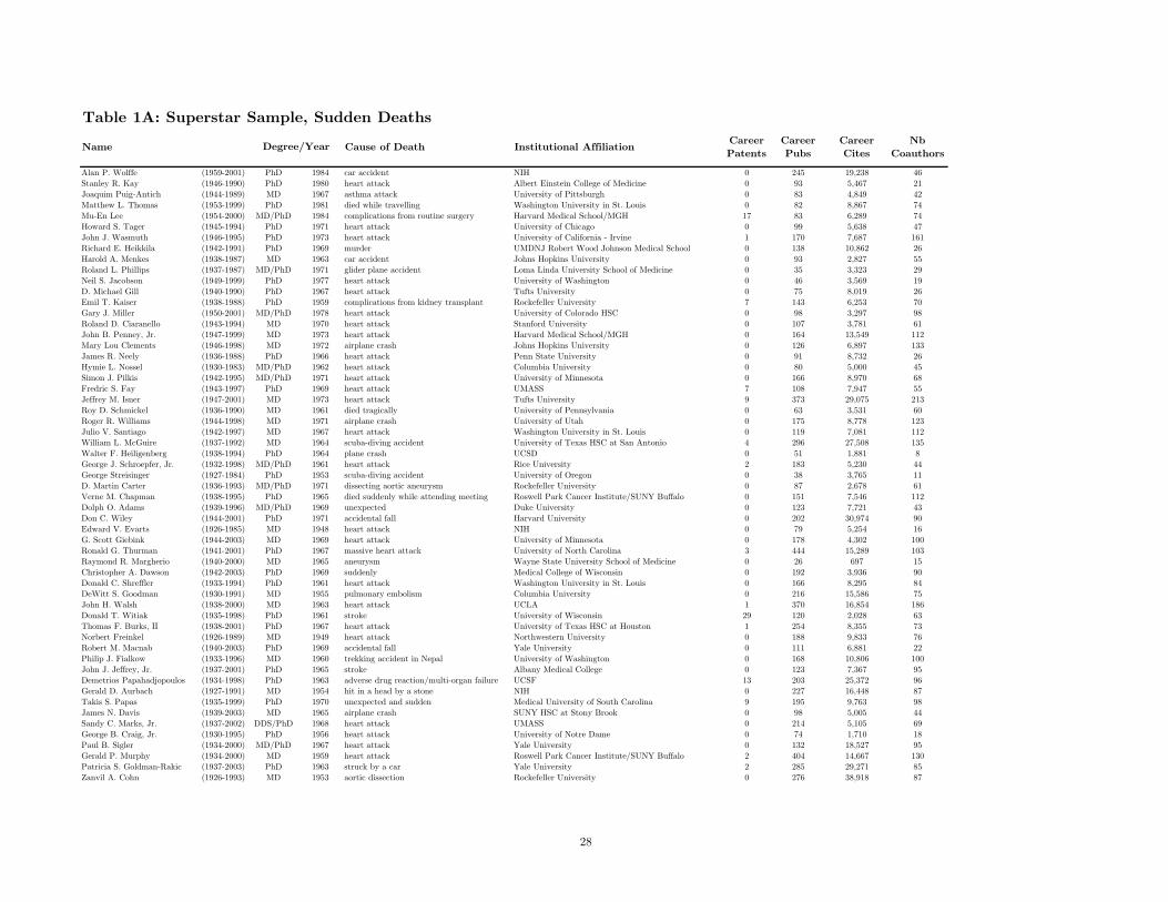
Table 1A: Superstar Sample, Sudden Deaths

Name Cause of Death Institutional AffiliationCareer Patents

Career Pubs

Career Cites

Nb Coauthors

Alan P. Wolffe (1959-2001) PhD 1984 car accident NIH 0 245 19,238 46Stanley R. Kay (1946-1990) PhD 1980 heart attack Albert Einstein College of Medicine 0 93 5,467 21Joaquim Puig-Antich (1944-1989) MD 1967 asthma attack University of Pittsburgh 0 83 4,849 42Matthew L. Thomas (1953-1999) PhD 1981 died while travelling Washington University in St. Louis 0 82 8,867 74Mu-En Lee (1954-2000) MD/PhD 1984 complications from routine surgery Harvard Medical School/MGH 17 83 6,289 74Howard S. Tager (1945-1994) PhD 1971 heart attack University of Chicago 0 99 5,638 47John J. Wasmuth (1946-1995) PhD 1973 heart attack University of California - Irvine 1 170 7,687 161Richard E. Heikkila (1942-1991) PhD 1969 murder UMDNJ Robert Wood Johnson Medical School 0 138 10,862 26Harold A. Menkes (1938-1987) MD 1963 car accident Johns Hopkins University 0 93 2,827 55Roland L. Phillips (1937-1987) MD/PhD 1971 glider plane accident Loma Linda University School of Medicine 0 35 3,323 29Neil S. Jacobson (1949-1999) PhD 1977 heart attack University of Washington 0 46 3,569 19D. Michael Gill (1940-1990) PhD 1967 heart attack Tufts University 0 75 8,019 26Emil T. Kaiser (1938-1988) PhD 1959 complications from kidney transplant Rockefeller University 7 143 6,253 70Gary J. Miller (1950-2001) MD/PhD 1978 heart attack University of Colorado HSC 0 98 3,297 98Roland D. Ciaranello (1943-1994) MD 1970 heart attack Stanford University 0 107 3,781 61John B. Penney, Jr. (1947-1999) MD 1973 heart attack Harvard Medical School/MGH 0 164 13,549 112Mary Lou Clements (1946-1998) MD 1972 airplane crash Johns Hopkins University 0 126 6,897 133James R. Neely (1936-1988) PhD 1966 heart attack Penn State University 0 91 8,732 26Hymie L. Nossel (1930-1983) MD/PhD 1962 heart attack Columbia University 0 80 5,000 45Simon J. Pilkis (1942-1995) MD/PhD 1971 heart attack University of Minnesota 0 166 8,970 68Fredric S. Fay (1943-1997) PhD 1969 heart attack UMASS 7 108 7,947 55Jeffrey M. Isner (1947-2001) MD 1973 heart attack Tufts University 9 373 29,075 213Roy D. Schmickel (1936-1990) MD 1961 died tragically University of Pennsylvania 0 63 3,531 60Roger R. Williams (1944-1998) MD 1971 airplane crash University of Utah 0 175 8,778 123Julio V. Santiago (1942-1997) MD 1967 heart attack Washington University in St. Louis 0 119 7,081 112William L. McGuire (1937-1992) MD 1964 scuba-diving accident University of Texas HSC at San Antonio 4 296 27,508 135Walter F. Heiligenberg (1938-1994) PhD 1964 plane crash UCSD 0 51 1,881 8George J. Schroepfer, Jr. (1932-1998) MD/PhD 1961 heart attack Rice University 2 183 5,230 44George Streisinger (1927-1984) PhD 1953 scuba-diving accident University of Oregon 0 38 3,765 11D. Martin Carter (1936-1993) MD/PhD 1971 dissecting aortic aneurysm Rockefeller University 0 87 2,678 61Verne M. Chapman (1938-1995) PhD 1965 died suddenly while attending meeting Roswell Park Cancer Institute/SUNY Buffalo 0 151 7,546 112Dolph O. Adams (1939-1996) MD/PhD 1969 unexpected Duke University 0 123 7,721 43Don C. Wiley (1944-2001) PhD 1971 accidental fall Harvard University 0 202 30,974 90Edward V. Evarts (1926-1985) MD 1948 heart attack NIH 0 79 5,254 16G. Scott Giebink (1944-2003) MD 1969 heart attack University of Minnesota 0 178 4,302 100Ronald G. Thurman (1941-2001) PhD 1967 massive heart attack University of North Carolina 3 444 15,289 103Raymond R. Margherio (1940-2000) MD 1965 aneurysm Wayne State University School of Medicine 0 26 697 15Christopher A. Dawson (1942-2003) PhD 1969 suddenly Medical College of Wisconsin 0 192 3,936 90Donald C. Shreffler (1933-1994) PhD 1961 heart attack Washington University in St. Louis 0 166 8,295 84DeWitt S. Goodman (1930-1991) MD 1955 pulmonary embolism Columbia University 0 216 15,586 75John H. Walsh (1938-2000) MD 1963 heart attack UCLA 1 370 16,854 186Donald T. Witiak (1935-1998) PhD 1961 stroke University of Wisconsin 29 120 2,028 63Thomas F. Burks, II (1938-2001) PhD 1967 heart attack University of Texas HSC at Houston 1 254 8,355 73Norbert Freinkel (1926-1989) MD 1949 heart attack Northwestern University 0 188 9,833 76Robert M. Macnab (1940-2003) PhD 1969 accidental fall Yale University 0 111 6,881 22Philip J. Fialkow (1933-1996) MD 1960 trekking accident in Nepal University of Washington 0 168 10,806 100John J. Jeffrey, Jr. (1937-2001) PhD 1965 stroke Albany Medical College 0 123 7,367 95Demetrios Papahadjopoulos (1934-1998) PhD 1963 adverse drug reaction/multi-organ failure UCSF 13 203 25,372 96Gerald D. Aurbach (1927-1991) MD 1954 hit in a head by a stone NIH 0 227 16,448 87Takis S. Papas (1935-1999) PhD 1970 unexpected and sudden Medical University of South Carolina 9 195 9,763 98James N. Davis (1939-2003) MD 1965 airplane crash SUNY HSC at Stony Brook 0 98 5,005 44Sandy C. Marks, Jr. (1937-2002) DDS/PhD 1968 heart attack UMASS 0 214 5,105 69George B. Craig, Jr. (1930-1995) PhD 1956 heart attack University of Notre Dame 0 74 1,710 18Paul B. Sigler (1934-2000) MD/PhD 1967 heart attack Yale University 0 132 18,527 95Gerald P. Murphy (1934-2000) MD 1959 heart attack Roswell Park Cancer Institute/SUNY Buffalo 2 404 14,667 130Patricia S. Goldman-Rakic (1937-2003) PhD 1963 struck by a car Yale University 2 285 29,271 85Zanvil A. Cohn (1926-1993) MD 1953 aortic dissection Rockefeller University 0 276 38,918 87

Degree/Year

28

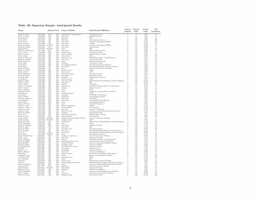
Table 1B: Superstar Sample, Anticipated Deaths

Name Cause of Death Institutional AffiliationCareer Patents

Career Pubs

Career Cites

Nb Coauthors

Richard C. Parker (1951-1986) PhD 1979 lymphoblastic T-cell lymphoma Columbia University 0 14 1,883 12Ernest G. Peralta (1959-1999) PhD 1986 brain cancer Harvard University 0 41 5,359 17George Khoury (1943-1987) MD 1970 lymphoma NIH 0 134 11,305 66B. Frank Polk (1942-1988) MD 1967 brain cancer Johns Hopkins University 0 107 8,226 121Joel D. Meyers (1944-1991) MD 1970 colon cancer University of Washington/FHCRC 0 171 14,717 120Melvin L. Marcus (1940-1989) MD 1966 colon cancer UMASS 0 225 15,034 96Harold Weintraub (1945-1995) MD/PhD 1973 brain cancer University of Washington/FHCRC 3 154 31,562 83Richard K. Gershon (1932-1983) MD 1959 lung cancer Yale University 0 182 12,007 73Markku Linnoila (1947-1998) MD/PhD 1974 cancer NIH 6 513 21,254 175Theodore S. Zimmerman (1937-1988) MD 1963 lung cancer Scripps Research Institute 20 132 12,264 75Larry C. Clark (1948-2000) PhD 1981 prostate cancer University of Arizona 1 33 2,387 33Robert F. Spencer (1949-2001) PhD 1974 gastric carcinoma Medical College of Virginia 0 59 2,136 25Janis V. Giorgi (1947-2000) PhD 1977 uterine cancer UCLA 1 130 10,212 137Samuel W. Perry, 3rd (1941-1994) MD 1967 pancreatic cancer Weill Medical College ˜ Cornell University 0 44 1,210 31Edward C. Franklin (1928-1982) MD 1950 brain cancer New York University 0 224 12,761 69Gerald T. Babcock (1946-2000) PhD 1973 cancer Michigan State University 0 123 8,511 49Lois K. Miller (1945-1999) PhD 1972 melanoma University of Georgia 9 120 8,261 20Tai-Shun Lin (1939-1994) PhD 1970 non hodgkin's lymphoma Yale University School of Medicine 19 91 3,102 42Ora M. Rosen (1935-1990) MD 1960 breast cancer Sloan Kettering Institute for Cancer Research 0 150 14,587 72Edwin H. Beachey (1934-1989) MD 1962 cancer University of Tennessee at Memphis 10 192 10,080 57Elizabeth A. Bates (1974-2003) PhD 1974 pancreatic cancer UCSD 0 81 1,985 18Helene S. Smith (1941-1997) PhD 1967 breast cancer UCSF 5 97 5,634 59Murray Rabinowitz (1927-1983) MD 1950 muscular dystrophy University of Chicago 0 146 8,229 51C. Richard Taylor (1939-1995) PhD 1963 heart failure Harvard University 0 100 6,377 26Norton B. Gilula (1944-2000) PhD 1971 lymphoma Scripps Research Institute 3 99 13,147 62Ira Herskowitz (1946-2003) PhD 1971 pancreatic cancer UCSF 4 159 17,457 85Bernard N. Fields (1938-1995) MD 1962 pancreatic cancer Harvard Medical School/Brigham & Women's Hospital 1 181 10,505 102Wallace P. Rowe (1926-1983) MD 1948 colon cancer NIH 0 232 21,432 79Allan C. Wilson (1934-1991) PhD 1961 leukemia UC Berkeley 0 164 25,915 48Priscilla A. Campbell (1940-1998) PhD 1968 cervical cancer University of Colorado HSC/Nat. Jewish center 0 77 3,914 31Laird S. Cermak (1942-1999) PhD 1968 leukemia Boston University 0 73 2,338 25Peter A. Kollman (1944-2001) PhD 1970 cancer UCSF 0 189 9,095 79Elizabeth M. Smith (1939-1997) PhD 1978 cancer Washington University School of Medicine 0 47 1,265 17Nelson Butters (1937-1995) PhD 1964 Lou Gehrig's disease UCSD 0 191 12,555 105Aaron Janoff (1930-1988) PhD 1959 long illness SUNY HSC at Stony Brook 0 131 8,590 58David G. Marsh (1940-1998) PhD 1964 glioblastoma Johns Hopkins University 1 142 6,395 58G. Harrison Echols, Jr. (1933-1993) PhD 1959 lung cancer UC Berkeley 0 112 9,190 56George Némethy (1934-1994) PhD 1962 brain cancer Mount Sinai School of Medicine 0 76 7,079 16Mette Strand (1937-1997) PhD 1964 cancer Johns Hopkins University 4 128 6,044 58Lawrence H. Piette (1932-1992) PhD 1957 cancer Utah State University 0 56 2,722 19William L. Chick (1938-1998) MD 1963 diabetes complications UMASS 0 90 5,108 70Charles A. Janeway, Jr. (1943-2003) MD 1969 B-cell lymphoma Yale University 0 313 31,455 141Howard M. Temin (1934-1994) PhD 1959 lung cancer University of Wisconsin 4 210 17,276 46Joachim G. Liehr (1942-2003) PhD 1968 pancreatic cancer University of Texas Medical Branch at Galveston 0 134 6,272 71Harvey D. Preisler (1941-2002) MD 1965 lymphoma Rush Medical College 0 304 7,069 107Keith Green (1940-2001) PhD 1964 died after lengthy illness Medical College of Georgia 0 206 2,572 44Donald J. Cohen (1940-2001) MD 1966 ocular melanoma Yale University 0 298 12,166 160Gregory Mooser (1942-2003) DDS/PhD 1972 complications from alzheimer's disease University of Southern California 0 23 962 9Roy H. Steinberg (1935-1997) MD/PhD 1965 multiple myeloma UCSF 3 121 6,707 25Thomas W. Smith (1936-1997) MD 1965 mesothelioma Harvard Medical School/Brigham & Women's Hospital 0 158 11,136 108John C. Liebeskind (1935-1997) PhD 1962 cancer UCLA 0 147 10,160 30Marian W. Fischman (1939-2001) PhD 1972 colon cancer Columbia University 0 157 5,910 42Richard J. Wyatt (1939-2002) MD 1964 lung cancer NIH 2 533 21,692 205Sydney E. Salmon (1936-1999) MD 1962 pancreatic cancer University of Arizona 8 286 20,024 204Sidney H. Ingbar (1925-1988) MD 1947 lung cancer Harvard Medical School/Beth Israel Medical Center 1 290 14,523 75Eva J. Neer (1937-2000) MD 1963 breast cancer Harvard Medical School/Brigham & Women's Hospital 0 104 10,652 60Kiichi Sagawa (1926-1989) MD/PhD 1958 cancer Johns Hopkins University 0 119 9,491 39Charles D. Heidelberger (1920-1983) PhD 1946 carcinoma of nasal sinus University of Southern California 0 242 19,302 59Robert J. Fass (1939-2002) MD 1964 lung cancer Ohio State University 0 132 3,703 77Gerald L. Klerman (1928-1992) MD 1954 diabetes Weill Medical College ˜ Cornell University 0 252 19,458 114Eleanor M. Saffran (1938-2002) PhD 1968 amyotrophic lateral sclerosis Temple University School of Medicine 0 41 2,811 14Merton Bernfield (1938-2002) MD 1961 Parkinson's Disease Harvard Medical School/Children's Hospital 8 137 11,962 87Richard P. Bunge (1932-1996) MD 1960 esophageal cancer University of Miami 0 157 10,828 70Irving Kupfermann (1938-2002) PhD 1964 Creutzfeldt-Jacob's disease Columbia University 0 120 7,635 23Jiri Palek (1934-1998) MD 1958 2 year illness Tufts University 0 127 5,487 51Harold C. Neu (1934-1998) MD 1960 glioblastoma Columbia University 1 530 18,498 102Edwin L. Bierman (1930-1995) MD 1955 bone cancer University of Washington 0 204 14,583 70Edgar Haber (1932-1997) MD 1956 multiple myeloma Harvard University School of Public Health 29 372 27,458 175Joseph Stokes, 3rd (1924-1989) MD 1949 cancer Boston University School of Medicine 0 62 2,815 46J. Christian Gillin (1938-2003) MD 1966 esophageal cancer UCSD 0 355 15,729 225Leo J. Neuringer (1928-1993) PhD 1957 cancer MIT 0 39 1,264 31Frank Lilly (1930-1995) PhD 1965 prostate cancer Albert Einstein College of Medicine 0 94 4,245 55Jane Pitt (1938-2003) MD 1964 chronic lymphocytic leukemia Columbia University College of Physicians and Surgeon 0 95 3,235 120Barbara H. Bowman (1930-1996) PhD 1959 cancer University of Texas Medical School at San Antonio 1 115 3,371 72Charlotte Friend (1921-1987) PhD 1950 lymphoma Mount Sinai School of Medicine 0 98 5,486 34Albert Dorfman (1916-1982) MD/PhD 1944 kidney failure University of Chicago 0 183 9,660 45William H. Tooley (1925-1992) MD 1949 long illness UCSF School of Medicine 0 77 5,890 62John R. Williamson (1934-2000) PhD 1959 cancer University of Pennsylvania School of Medicine 0 178 13,661 86Henry S. Kaplan (1918-1984) MD 1940 lung cancer Stanford University School of Medicine 3 395 27,480 132Charles G. Moertel (1927-1994) MD 1953 Hodgkin's Disease Mayo Medical School 0 290 21,372 166

Degree/Year

29

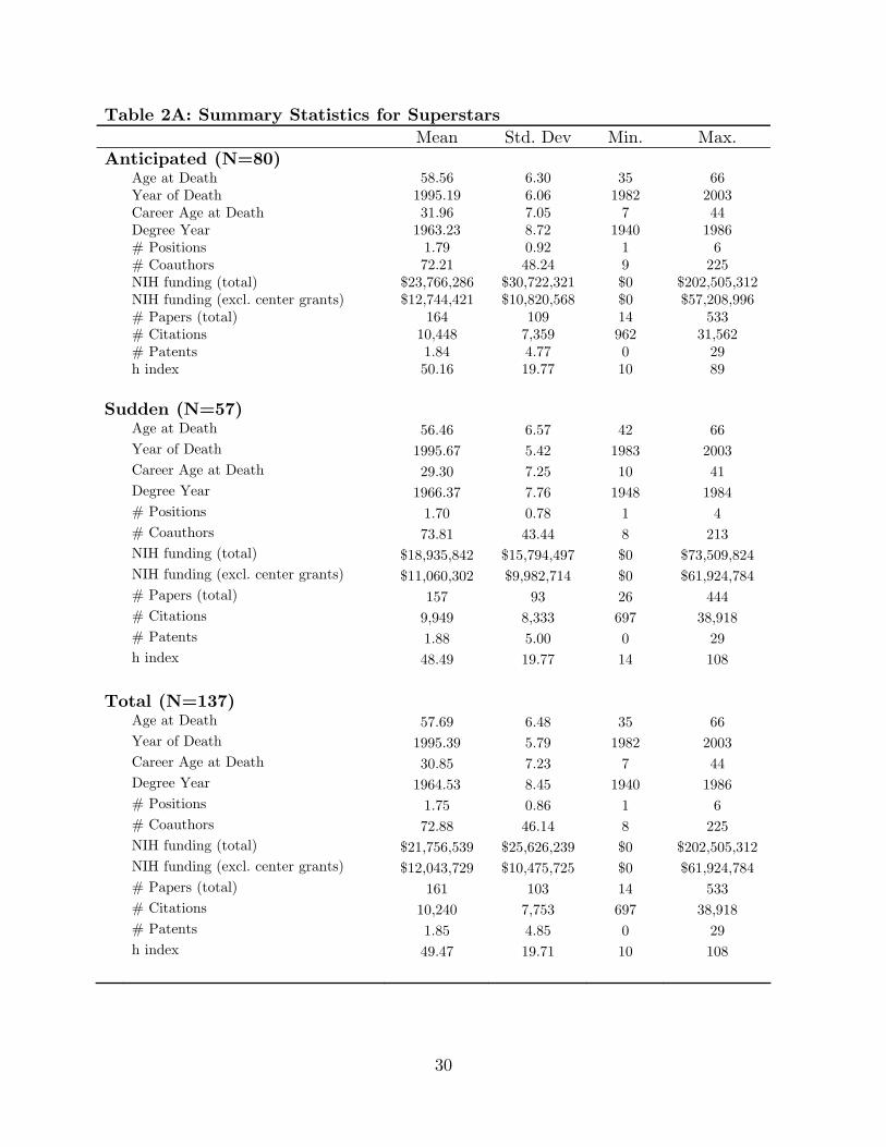
30

Table 2A: Summary Statistics for Superstars Mean Std. Dev Min. Max. Anticipated (N=80) Age at Death 58.56 6.30 35 66 Year of Death 1995.19 6.06 1982 2003 Career Age at Death 31.96 7.05 7 44 Degree Year 1963.23 8.72 1940 1986 # Positions 1.79 0.92 1 6 # Coauthors 72.21 48.24 9 225 NIH funding (total) $23,766,286 $30,722,321 $0 $202,505,312 NIH funding (excl. center grants) $12,744,421 $10,820,568 $0 $57,208,996 # Papers (total) 164 109 14 533 # Citations 10,448 7,359 962 31,562 # Patents 1.84 4.77 0 29 h index 50.16 19.77 10 89

Sudden (N=57) Age at Death 56.46 6.57 42 66

Year of Death 1995.67 5.42 1983 2003

Career Age at Death 29.30 7.25 10 41

Degree Year 1966.37 7.76 1948 1984

# Positions 1.70 0.78 1 4

# Coauthors 73.81 43.44 8 213

NIH funding (total) $18,935,842 $15,794,497 $0 $73,509,824

NIH funding (excl. center grants) $11,060,302 $9,982,714 $0 $61,924,784

# Papers (total) 157 93 26 444

# Citations 9,949 8,333 697 38,918

# Patents 1.88 5.00 0 29

h index 48.49 19.77 14 108

Total (N=137) Age at Death 57.69 6.48 35 66

Year of Death 1995.39 5.79 1982 2003

Career Age at Death 30.85 7.23 7 44

Degree Year 1964.53 8.45 1940 1986

# Positions 1.75 0.86 1 6

# Coauthors 72.88 46.14 8 225

NIH funding (total) $21,756,539 $25,626,239 $0 $202,505,312

NIH funding (excl. center grants) $12,043,729 $10,475,725 $0 $61,924,784

# Papers (total) 161 103 14 533

# Citations 10,240 7,753 697 38,918

# Patents 1.85 4.85 0 29

h index 49.47 19.71 10 108

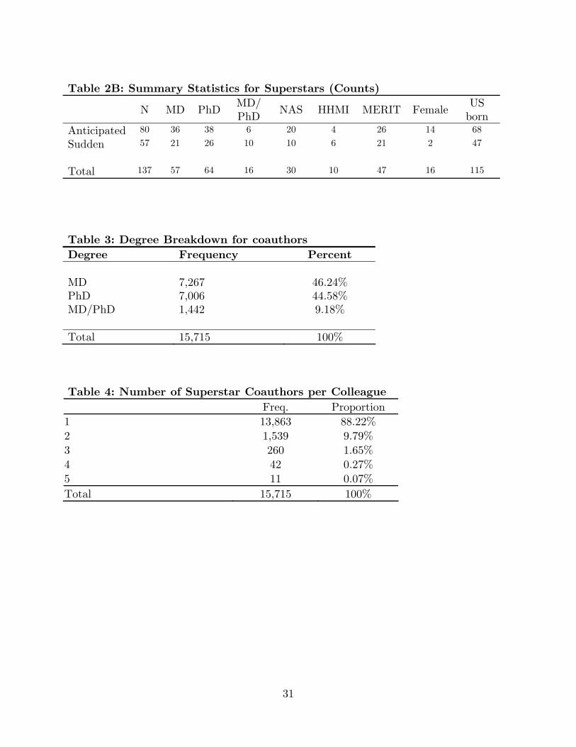
31

Table 2B: Summary Statistics for Superstars (Counts)

N MD PhD MD/ PhD

NAS HHMI MERIT Female US

born Anticipated 80 36 38 6 20 4 26 14 68

Sudden 57 21 26 10 10 6 21 2 47

Total 137 57 64 16 30 10 47 16 115

Table 3: Degree Breakdown for coauthors Degree Frequency Percent MD 7,267 46.24% PhD 7,006 44.58% MD/PhD 1,442 9.18% Total 15,715 100% Table 4: Number of Superstar Coauthors per Colleague

Freq. Proportion 1 13,863 88.22% 2 1,539 9.79% 3 260 1.65% 4 42 0.27% 5 11 0.07% Total 15,715 100%

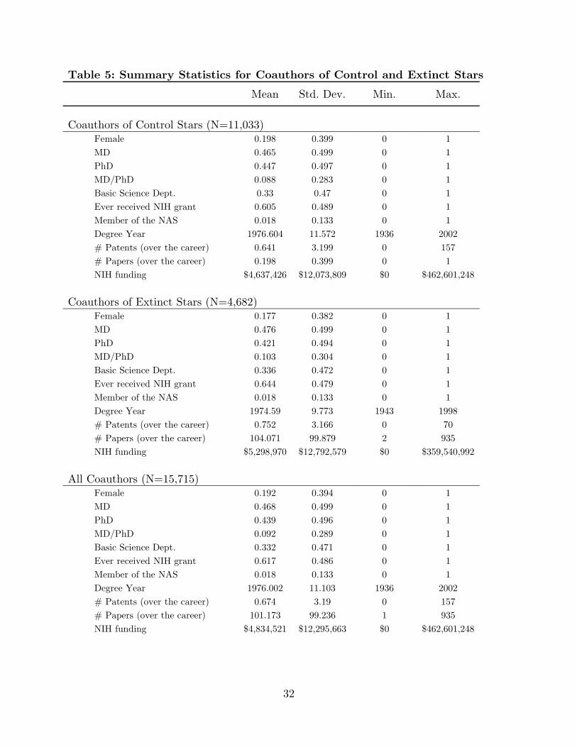
32

Table 5: Summary Statistics for Coauthors of Control and Extinct Stars

Mean Std. Dev. Min. Max.

Coauthors of Control Stars (N=11,033) Female 0.198 0.399 0 1

MD 0.465 0.499 0 1

PhD 0.447 0.497 0 1

MD/PhD 0.088 0.283 0 1

Basic Science Dept. 0.33 0.47 0 1

Ever received NIH grant 0.605 0.489 0 1

Member of the NAS 0.018 0.133 0 1

Degree Year 1976.604 11.572 1936 2002

# Patents (over the career) 0.641 3.199 0 157

# Papers (over the career) 0.198 0.399 0 1

NIH funding $4,637,426 $12,073,809 $0 $462,601,248

Coauthors of Extinct Stars (N=4,682) Female 0.177 0.382 0 1

MD 0.476 0.499 0 1

PhD 0.421 0.494 0 1

MD/PhD 0.103 0.304 0 1

Basic Science Dept. 0.336 0.472 0 1

Ever received NIH grant 0.644 0.479 0 1

Member of the NAS 0.018 0.133 0 1

Degree Year 1974.59 9.773 1943 1998

# Patents (over the career) 0.752 3.166 0 70

# Papers (over the career) 104.071 99.879 2 935

NIH funding $5,298,970 $12,792,579 $0 $359,540,992

All Coauthors (N=15,715) Female 0.192 0.394 0 1

MD 0.468 0.499 0 1

PhD 0.439 0.496 0 1

MD/PhD 0.092 0.289 0 1

Basic Science Dept. 0.332 0.471 0 1

Ever received NIH grant 0.617 0.486 0 1

Member of the NAS 0.018 0.133 0 1

Degree Year 1976.002 11.103 1936 2002

# Patents (over the career) 0.674 3.19 0 157

# Papers (over the career) 101.173 99.236 1 935

NIH funding $4,834,521 $12,295,663 $0 $462,601,248

33

Table 6: Summary Statistics for Superstar/Colleague Dyads Mean Std. Dev Min. Max. Anticipated (N=4,303) JIF-weighted Papers (w/o star) 450.674 569.065 0.311 5705.146 JIF-weighted Papers (total) 542.481 645.322 1.246 6293.937 Non-weighted Papers (total) 140.198 131.307 2 1002 # Coauthorships 3.117 5.935 1 112 Trainee of star 0.083 0.276 0 1 Coauthor is senior to star 0.037 0.188 0 1 R01 grant at time of death 0.547 0.498 0 1 Career age at time of death 22.688 8.936 5 40 Same school at time of death 0.244 0.429 0 1 Within 10 miles at time of death 0.278 0.448 0 1

At least 1 coauthorship in 5 years prior to death 0.347 0.476 0 1

Sudden (N=3,089) JIF-weighted Papers (w/o star) 475.036 581.844 0.388 5067.218

JIF-weighted Papers (total) 556.654 651.196 1.378 6293.937

Non-weighted Papers (total) 142.299 134.428 2 1002

# Coauthorships 3.196 6.261 1 99

Trainee of star 0.073 0.26 0 1

Coauthor is senior to star 0.06 0.237 0 1

R01 grant at time of death 0.564 0.496 0 1

Career age at time of death 22.205 8.745 5 40

Same school at time of death 0.211 0.408 0 1

Within 10 miles at time of death 0.216 0.411 0 1

At least 1 coauthorship in 5 years prior to death 0.36 0.48 0 1

Total (N=7,392) JIF-weighted Papers (w/o star) 460.854 574.526 0.311 5705.146

JIF-weighted Papers (total) 548.404 647.777 1.246 6293.937

Non-weighted Papers (total) 141.076 132.615 2 1002

# Coauthorships 3.15 6.073 1 112

Trainee of star 0.079 0.269 0 1

Coauthor is senior to star 0.046 0.21 0 1

R01 grant at time of death 0.554 0.497 0 1

Career age at time of death 22.486 8.859 5 40

Same school at time of death 0.23 0.421 0 1

Within 10 miles at time of death 0.252 0.434 0 1

At least 1 coauthorship in 5 years prior to death 0.353 0.478 0 1

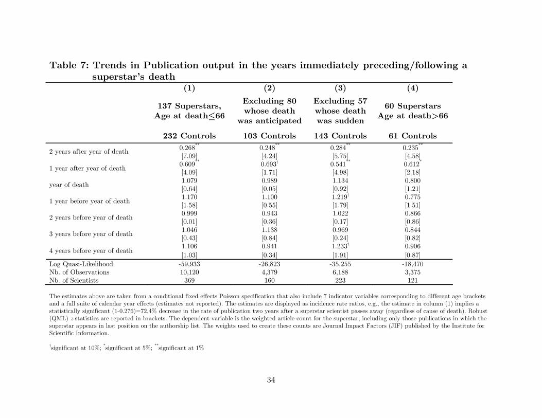
34

Table 7: Trends in Publication output in the years immediately preceding/following a

superstar’s death (1) (2) (3) (4)

137 Superstars, Age at death≤66

Excluding 80 whose death

was anticipated

Excluding 57 whose death was sudden

60 Superstars Age at death>66

232 Controls 103 Controls 143 Controls 61 Controls 0.268** 0.248** 0.284** 0.235** 2 years after year of death [7.09] [4.24] [5.75] [4.58] 0.609** 0.693† 0.541** 0.612* 1 year after year of death [4.09] [1.71] [4.98] [2.18] 1.079 0.989 1.134 0.800 year of death [0.64] [0.05] [0.92] [1.21] 1.170 1.100 1.219† 0.775 1 year before year of death [1.58] [0.55] [1.79] [1.51] 0.999 0.943 1.022 0.866 2 years before year of death [0.01] [0.36] [0.17] [0.86] 1.046 1.138 0.969 0.844 3 years before year of death [0.43] [0.84] [0.24] [0.82] 1.106 0.941 1.233† 0.906

4 years before year of death [1.03] [0.34] [1.91] [0.87]

Log Quasi-Likelihood -59,933 -26,823 -35,255 -18,470 Nb. of Observations 10,120 4,379 6,188 3,375 Nb. of Scientists 369 160 223 121 The estimates above are taken from a conditional fixed effects Poisson specification that also include 7 indicator variables corresponding to different age brackets and a full suite of calendar year effects (estimates not reported). The estimates are displayed as incidence rate ratios, e.g., the estimate in column (1) implies a statistically significant (1-0.276)=72.4% decrease in the rate of publication two years after a superstar scientist passes away (regardless of cause of death). Robust (QML) z-statistics are reported in brackets. The dependent variable is the weighted article count for the superstar, including only those publications in which the superstar appears in last position on the authorship list. The weights used to create these counts are Journal Impact Factors (JIF) published by the Institute for Scientific Information. †significant at 10%; *significant at 5%; **significant at 1%

35

Table 8: Impact of Superstar Death on Coauthors’ Publication Rates Panel A: Treatment Dyads Only, JIF-weighted Total Publications

(1) (2) (3) (4) (5) (6) All All Sudden Sudden Anticip. Anticip.

0.929** 0.932** 0.895** 0.914** 0.959† 0.947* After Death [4.01] [3.60] [4.11] [2.96] [1.75] [2.13] After Death × 1.008 0.907* 1.084* Regular Collab. [0.25] [2.00] [1.96]

After Death × 0.926 0.954 0.911 Close Collab. [1.52] [0.85] [1.22]

Log Quasi-Likelihood -1,271,471 -1,271,339 -531,709 -531,503 -738,531 -738,173

Nb. of Obs. 191,046 191,046 79,232 79,232 111,814 111,814

Nb. of Dyads 7,392 7,392 3,089 3,089 4,303 4,303

Nb. of Superstars 137 137 57 57 80 80

Panel B: Treatment Dyads Only, JIF-weighted Publications written with others

(1) (2) (3) (4) (5) (6) All All Sudden Sudden Anticip. Anticip.

0.964* 0.941** 0.922** 0.919** 1.000 0.959† After Death [2.06] [3.25] [3.17] [2.88] [0.01] [1.72] After Death × 1.059† 0.949 1.142** Regular Collab. [1.76] [1.09] [3.12]

After Death × 1.201** 1.256** 1.168* Close Collab. [3.51] [3.71] [2.01]

Log Quasi-Likelihood -1,246,076 -1,245,380 -520,674 -520,189 -724,236 -723,539

Nb. of Obs. 191,046 191,046 79,232 79,232 111,814 111,814

Nb. of Dyads 7,392 7,392 3,089 3,089 4,303 4,303

Nb. of Superstars 137 137 57 57 80 80 Estimates are displayed as incidence rate ratios (exponentiated coefficients). For example. the estimates in column (4) of Panel A imply that casual coauthors suffer a statistically significant (1-0.914)=8.6% decrease in the rate of publication after one’s superstar coauthor passes away, but that regular coauthors (between 3 and 9 publications) incur an additional decrease of 1-0.910)=9%. All models incorporate year effects and seven age category indicator variables (career age less than 5 years is the omitted category). Absolute value of robust (QML) z-statistics in brackets, clustered at the level of the superstar. †significant at 10%; *significant at 5%; **significant at 1%.

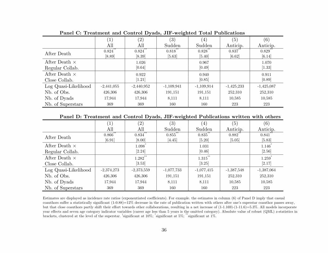
36

Panel C: Treatment and Control Dyads, JIF-weighted Total Publications (1) (2) (3) (4) (5) (6) All All Sudden Sudden Anticip. Anticip.

0.824** 0.824** 0.818** 0.828** 0.837** 0.829** After Death [8.89] [8.39] [5.63] [5.40] [6.62] [6.14] After Death × 1.026 0.967 1.070 Regular Collab. [0.64] [0.49] [1.33]

After Death × 0.922 0.940 0.911 Close Collab. [1.21] [0.85] [0.89]

Log Quasi-Likelihood -2,441,055 -2,440,952 -1,109,941 -1,109,914 -1,425,233 -1,425,087

Nb. of Obs. 426,306 426,306 191,151 191,151 252,310 252,310

Nb. of Dyads 17,944 17,944 8,111 8,111 10,585 10,585

Nb. of Superstars 369 369 160 160 223 223

Panel D: Treatment and Control Dyads, JIF-weighted Publications written with others

(1) (2) (3) (4) (5) (6) All All Sudden Sudden Anticip. Anticip.

0.866** 0.834** 0.855** 0.835** 0.882** 0.841** After Death [6.91] [8.00] [4.45] [5.20] [5.05] [5.83] After Death × 1.098* 1.031 1.146* Regular Collab. [2.24] [0.46] [2.56]

After Death × 1.282** 1.315** 1.259* Close Collab. [3.53] [3.25] [2.17]

Log Quasi-Likelihood -2,374,273 -2,373,559 -1,077,733 -1,077,415 -1,387,548 -1,387,064

Nb. of Obs. 426,306 426,306 191,151 191,151 252,310 252,310

Nb. of Dyads 17,944 17,944 8,111 8,111 10,585 10,585

Nb. of Superstars 369 369 160 160 223 223 Estimates are displayed as incidence rate ratios (exponentiated coefficients). For example. the estimates in column (6) of Panel D imply that casual coauthors suffer a statistically significant (1-0.88)=12% decrease in the rate of publication written with others after one’s superstar coauthor passes away, but that close coauthors partly shift their effort towards other collaborations, resulting in a net increase of (1-1.169)-(1-11.6)=5.3%. All models incorporate year effects and seven age category indicator variables (career age less than 5 years is the omitted category). Absolute value of robust (QML) z-statistics in brackets, clustered at the level of the superstar. †significant at 10%; *significant at 5%; **significant at 1%.

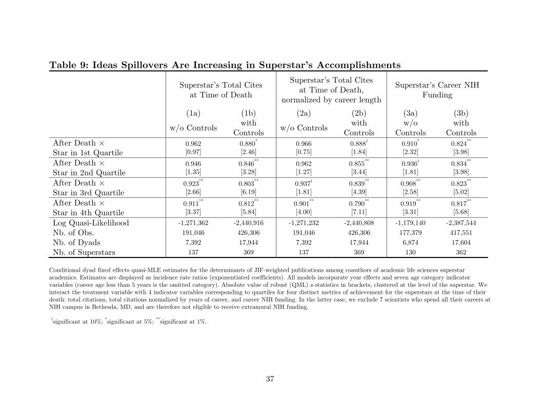
37

Table 9: Ideas Spillovers Are Increasing in Superstar’s Accomplishments

Superstar’s Total Cites at Time of Death

Superstar’s Total Cites at Time of Death,

normalized by career length

Superstar’s Career NIH Funding

(1a) (1b) (2a) (2b) (3a) (3b)

w/o Controls with Controls w/o Controls with

Controls w/o

Controls with

Controls After Death × 0.962 0.880* 0.966 0.888† 0.910* 0.824** Star in 1st Quartile [0.97] [2.46] [0.75] [1.84] [2.32] [3.98]

After Death × 0.946 0.846** 0.962 0.855** 0.936† 0.834** Star in 2nd Quartile [1.35] [3.28] [1.27] [3.44] [1.81] [3.98]

After Death × 0.923** 0.803** 0.937† 0.839** 0.908** 0.823** Star in 3rd Quartile [2.66] [6.19] [1.81] [4.39] [2.58] [5.02]

After Death × 0.911** 0.812** 0.901** 0.790** 0.919** 0.817** Star in 4th Quartile [3.37] [5.84] [4.00] [7.11] [3.31] [5.68]

Log Quasi-Likelihood -1,271,362 -2,440,916 -1,271,232 -2,440,808 -1,179,140 -2,387,544

Nb. of Obs. 191,046 426,306 191,046 426,306 177,379 417,551

Nb. of Dyads 7,392 17,944 7,392 17,944 6,874 17,604

Nb. of Superstars 137 369 137 369 130 362 Conditional dyad fixed effects quasi-MLE estimates for the determinants of JIF-weighted publications among coauthors of academic life sciences superstar academics. Estimates are displayed as incidence rate ratios (exponentiated coefficients). All models incorporate year effects and seven age category indicator variables (career age less than 5 years is the omitted category). Absolute value of robust (QML) z-statistics in brackets, clustered at the level of the superstar. We interact the treatment variable with 4 indicator variables corresponding to quartiles for four distinct metrics of achievement for the superstars at the time of their death: total citations, total citations normalized by years of career, and career NIH funding. In the latter case, we exclude 7 scientists who spend all their careers at NIH campus in Bethesda, MD, and are therefore not eligible to receive extramural NIH funding. †significant at 10%; *significant at 5%; **significant at 1%.

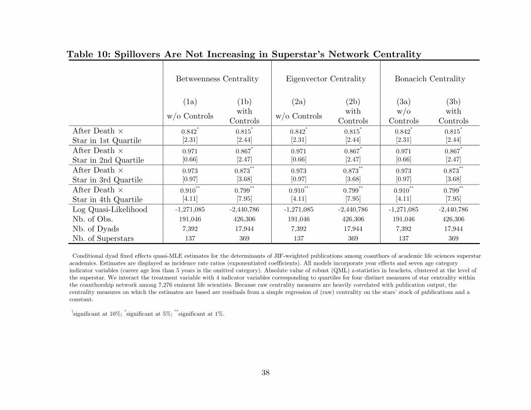
38

Table 10: Spillovers Are Not Increasing in Superstar’s Network Centrality

Betweenness Centrality Eigenvector Centrality Bonacich Centrality

(1a) (1b) (2a) (2b) (3a) (3b)

w/o Controlswith

Controls w/o Controls with

Controls w/o

Controls with

Controls After Death × 0.842* 0.815* 0.842* 0.815* 0.842* 0.815* Star in 1st Quartile [2.31] [2.44] [2.31] [2.44] [2.31] [2.44]

After Death × 0.971 0.867* 0.971 0.867* 0.971 0.867* Star in 2nd Quartile [0.66] [2.47] [0.66] [2.47] [0.66] [2.47]

After Death × 0.973 0.873** 0.973 0.873** 0.973 0.873** Star in 3rd Quartile [0.97] [3.68] [0.97] [3.68] [0.97] [3.68]

After Death × 0.910** 0.799** 0.910** 0.799** 0.910** 0.799** Star in 4th Quartile [4.11] [7.95] [4.11] [7.95] [4.11] [7.95]

Log Quasi-Likelihood -1,271,085 -2,440,786 -1,271,085 -2,440,786 -1,271,085 -2,440,786

Nb. of Obs. 191,046 426,306 191,046 426,306 191,046 426,306

Nb. of Dyads 7,392 17,944 7,392 17,944 7,392 17,944

Nb. of Superstars 137 369 137 369 137 369

Conditional dyad fixed effects quasi-MLE estimates for the determinants of JIF-weighted publications among coauthors of academic life sciences superstar academics. Estimates are displayed as incidence rate ratios (exponentiated coefficients). All models incorporate year effects and seven age category indicator variables (career age less than 5 years is the omitted category). Absolute value of robust (QML) z-statistics in brackets, clustered at the level of the superstar. We interact the treatment variable with 4 indicator variables corresponding to quartiles for four distinct measures of star centrality within the coauthorship network among 7,276 eminent life scientists. Because raw centrality measures are heavily correlated with publication output, the centrality measures on which the estimates are based are residuals from a simple regression of (raw) centrality on the stars’ stock of publications and a constant. †significant at 10%; *significant at 5%; **significant at 1%.

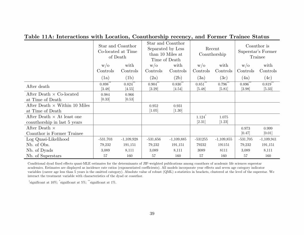
39

Table 11A: Interactions with Location, Coauthorship recency, and Former Trainee Status

Star and Coauthor Co-located at Time

of Death

Star and Coauthor Separated by Less than 10 Miles at Time of Death

Recent Coauthorship

Coauthor is Superstar’s Former

Trainee

w/o Controls

with Controls

w/o Controls

with Controls

w/o Controls

with Controls

w/o Controls

with Controls

(1a) (1b) (2a) (2b) (3a) (3c) (4a) (4c) 0.898** 0.824** 0.904** 0.830** 0.851** 0.796** 0.896** 0.819** After death [3.48] [4.55] [3.29] [4.54] [5.48] [5.81] [3.98] [5.33]

After Death × Co-located 0.984 0.966 at Time of Death [0.33] [0.53]

After Death × Within 10 Miles 0.952 0.931 at Time of Death [1.05] [1.30]

After Death × At least one 1.124* 1.075 coauthorship in last 5 years [2.31] [1.23]

After Death × 0.973 0.999 Coauthor is Former Trainee [0.47] [0.01]

Log Quasi-Likelihood -531,703 -1,109,928 -531,656 -1,109,885 -531255 -1,109,855 -531,705 -1,109,941

Nb. of Obs. 79,232 191,151 79,232 191,151 79232 191151 79,232 191,151

Nb. of Dyads 3,089 8,111 3,089 8,111 3089 8111 3,089 8,111

Nb. of Superstars 57 160 57 160 57 160 57 160

Conditional dyad fixed effects quasi-MLE estimates for the determinants of JIF-weighted publications among coauthors of academic life sciences superstar academics. Estimates are displayed as incidence rate ratios (exponentiated coefficients). All models incorporate year effects and seven age category indicator variables (career age less than 5 years is the omitted category). Absolute value of robust (QML) z-statistics in brackets, clustered at the level of the superstar. We interact the treatment variable with characteristics of the dyad or coauthor.

†significant at 10%; *significant at 5%; **significant at 1%.

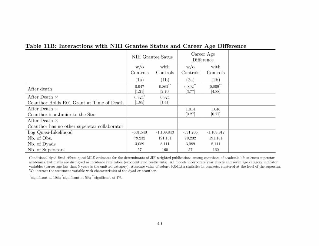
40

Table 11B: Interactions with NIH Grantee Status and Career Age Difference

NIH Grantee Satus Career Age Difference

w/o

Controls with

Controls w/o

Controls with

Controls

(1a) (1b) (2a) (2b) 0.947 0.862** 0.892** 0.809** After death [1.21] [2.70] [3.77] [4.88]

After Death × 0.924† 0.924 Coauthor Holds R01 Grant at Time of Death [1.85] [1.41]

After Death × 1.014 1.046 Coauthor is a Junior to the Star [0.27] [0.77]

After Death × Coauthor has no other superstar collaborator

Log Quasi-Likelihood -531,540 -1,109,843 -531,705 -1,109,917

Nb. of Obs. 79,232 191,151 79,232 191,151

Nb. of Dyads 3,089 8,111 3,089 8,111

Nb. of Superstars 57 160 57 160

Conditional dyad fixed effects quasi-MLE estimates for the determinants of JIF-weighted publications among coauthors of academic life sciences superstar academics. Estimates are displayed as incidence rate ratios (exponentiated coefficients). All models incorporate year effects and seven age category indicator variables (career age less than 5 years is the omitted category). Absolute value of robust (QML) z-statistics in brackets, clustered at the level of the superstar. We interact the treatment variable with characteristics of the dyad or coauthor.

†significant at 10%; *significant at 5%; **significant at 1%.

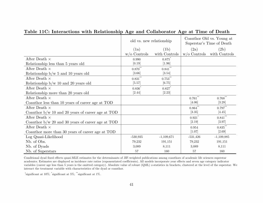
41

Table 11C: Interactions with Relationship Age and Collaborator Age at Time of Death

old vs. new relationship Coauthor Old vs. Young at Superstar’s Time of Death

(1a) (1b) (2a) (2b) w/o Controls with Controls w/o Controls with Controls After Death × 0.990 0.875* Relationship less than 5 years old [0.19] [1.96]

After Death × 0.870** 0.841** Relationship b/w 5 and 10 years old [3.66] [3.54]

After Death × 0.831** 0.753** Relationship b/w 10 and 20 years old [5.57] [6.75]

After Death × 0.836* 0.827* Relationship more than 20 years old [2.44] [2.23]

After Death × 0.761** 0.768** Coauthor less than 10 years of career age at TOD [4.06] [3.28]

After Death × 0.864** 0.797** Coauthor b/w 10 and 20 years of career age at TOD [3.35] [4.45]

After Death × 0.921* 0.841** Coauthor b/w 20 and 30 years of career age at TOD [2.19] [3.97]

After Death × 0.954 0.835** Coauthor more than 30 years of career age at TOD [1.07] [2.69]

Log Quasi-Likelihood -530,935 -1,109,671 -531,426 -1,109,885

Nb. of Obs. 79,232 191,151 79,232 191,151

Nb. of Dyads 3,089 8,111 3,089 8,111

Nb. of Superstars 57 160 57 160

Conditional dyad fixed effects quasi-MLE estimates for the determinants of JIF-weighted publications among coauthors of academic life sciences superstar academics. Estimates are displayed as incidence rate ratios (exponentiated coefficients). All models incorporate year effects and seven age category indicator variables (career age less than 5 years is the omitted category). Absolute value of robust (QML) z-statistics in brackets, clustered at the level of the superstar. We interact the treatment variable with characteristics of the dyad or coauthor.

†significant at 10%; *significant at 5%; **significant at 1%.

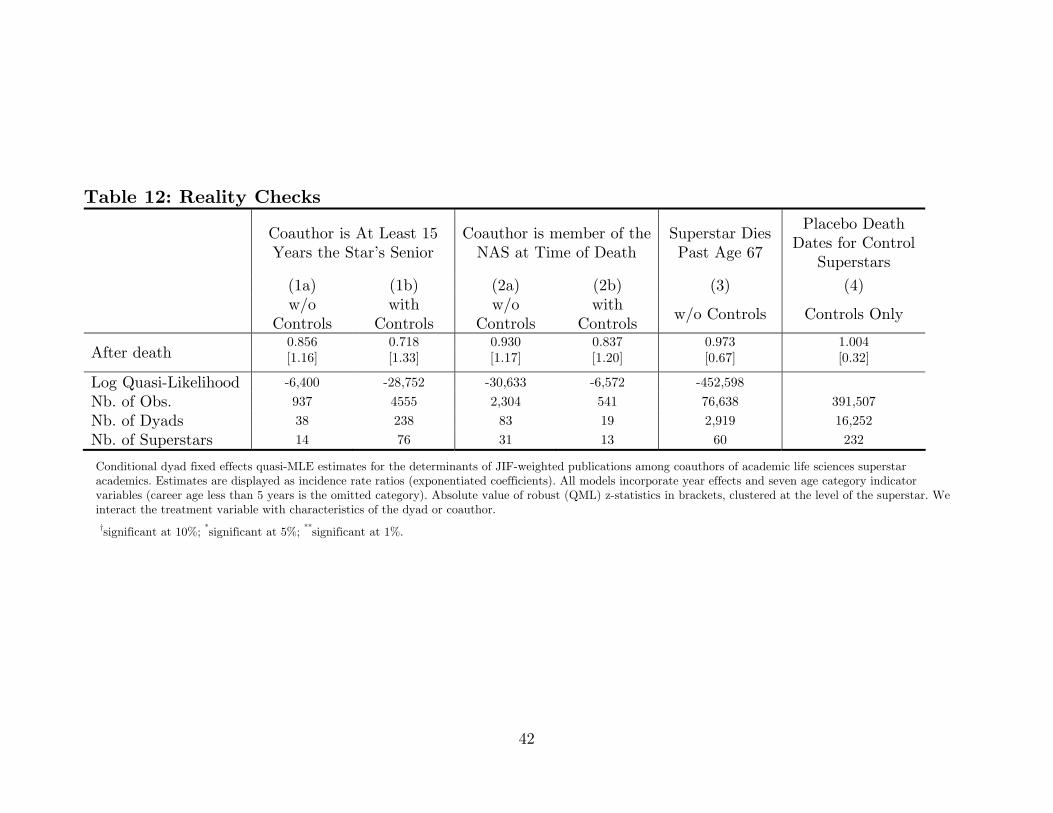
42

Table 12: Reality Checks

Coauthor is At Least 15 Years the Star’s Senior

Coauthor is member of the NAS at Time of Death

Superstar DiesPast Age 67

Placebo Death Dates for Control

Superstars (1a) (1b) (2a) (2b) (3) (4)

w/o

Controls with

Controls w/o

Controls with

Controls w/o Controls Controls Only

0.856 0.718 0.930 0.837 0.973 1.004 After death [1.16] [1.33] [1.17] [1.20] [0.67] [0.32]

Log Quasi-Likelihood -6,400 -28,752 -30,633 -6,572 -452,598

Nb. of Obs. 937 4555 2,304 541 76,638 391,507

Nb. of Dyads 38 238 83 19 2,919 16,252

Nb. of Superstars 14 76 31 13 60 232

Conditional dyad fixed effects quasi-MLE estimates for the determinants of JIF-weighted publications among coauthors of academic life sciences superstar academics. Estimates are displayed as incidence rate ratios (exponentiated coefficients). All models incorporate year effects and seven age category indicator variables (career age less than 5 years is the omitted category). Absolute value of robust (QML) z-statistics in brackets, clustered at the level of the superstar. We interact the treatment variable with characteristics of the dyad or coauthor.

†significant at 10%; *significant at 5%; **significant at 1%.

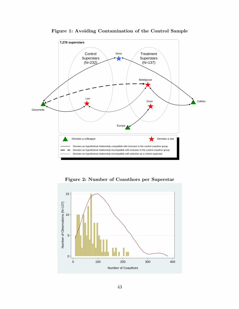
43

Figure 1: Avoiding Contamination of the Control Sample

7,276 superstars

TreatmentSuperstars

(N=137)

ControlSuperstars

(N=232)

Ganymede

Sirius

Betelgeuse

LeoCallistoOrion

Europa

Denotes a colleague Denotes a star

Denotes an hypothetical relationship compatible with inclusion in the control coauthor groupDenotes an hypothetical relationship incompatible with inclusion in the control coauthor groupDenotes an hypothetical relationship incompatible with selection as a control superstar

Figure 2: Number of Coauthors per Superstar

0

5

10

15

Num

ber o

f Obs

erva

tions

(N=1

37)

0 100 200 300 400

Number of Coauthors

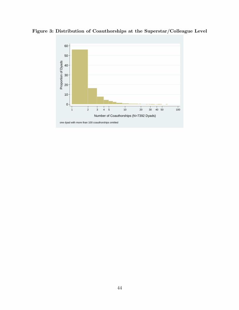
44

Figure 3: Distribution of Coauthorships at the Superstar/Colleague Level

0

10

20

30

40

50

60

Prop

ortio

n of

Dya

ds

1 2 3 4 5 10 20 30 40 50 100

Number of Coauthorships (N=7392 Dyads) one dyad with more than 100 coauthorships omitted

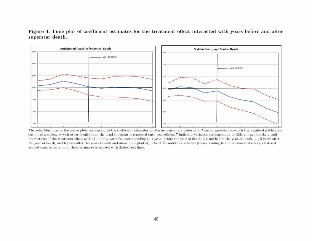
45

Figure 4: Time plot of coefficient estimates for the treatment effect interacted with years before and after superstar death.

The solid blue lines in the above plots correspond to the coefficient estimates for the incidence rate ratios of a Poisson regression in which the weighted publication output of a colleague with other faculty than the dead superstar is regressed onto year effects, 7 indicator variables corresponding to different age brackets, and interactions of the treatment effect with 11 dummy variables corresponding to 4 years before the year of death, 3 years before the year of death,…, 5 years after the year of death, and 6 years after the year of death and above (not plotted). The 95% confidence interval (corresponding to robust standard errors, clustered around supertsras) around these estimates is plotted with dashed red lines.

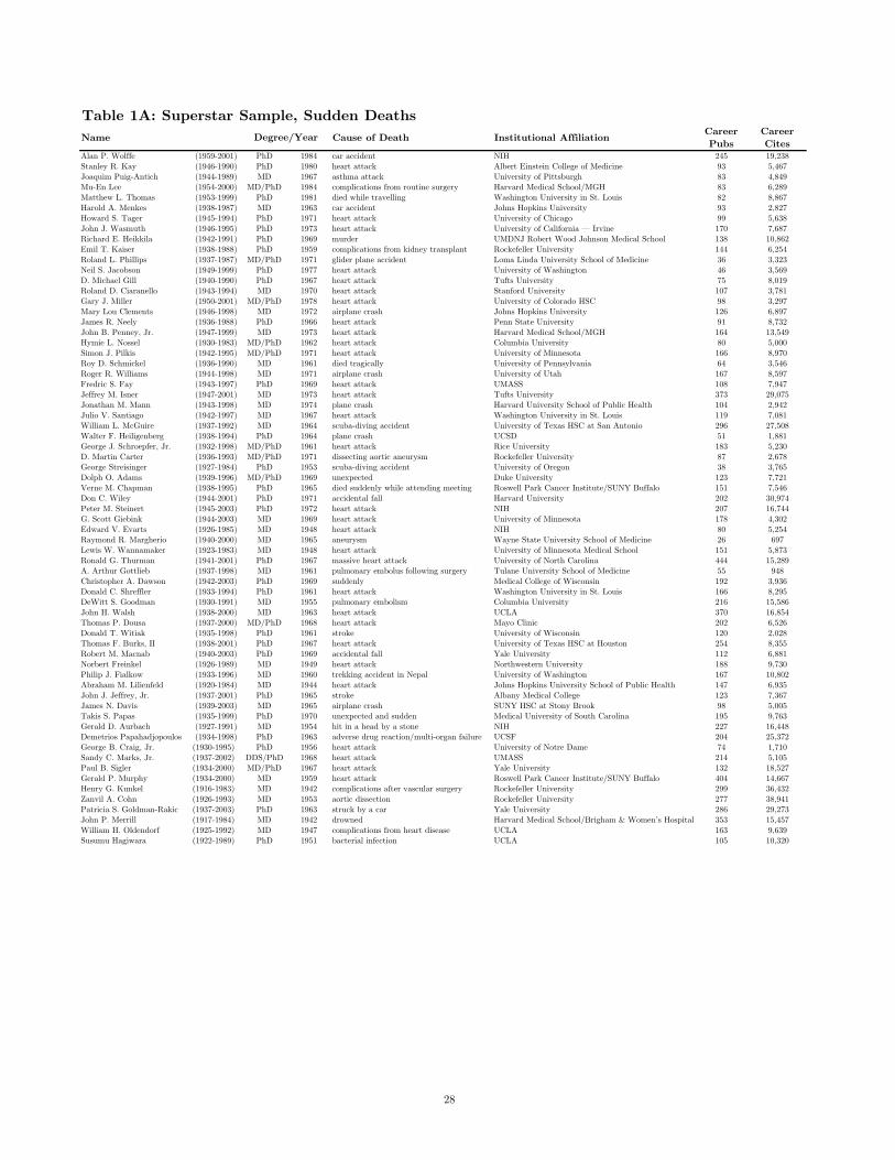
Table 1A: Superstar Sample, Sudden DeathsName Cause of Death Institutional Affiliation

Career Pubs

Career Cites

Alan P. Wolffe (1959-2001) PhD 1984 car accident NIH 245 19,238Stanley R. Kay (1946-1990) PhD 1980 heart attack Albert Einstein College of Medicine 93 5,467Joaquim Puig-Antich (1944-1989) MD 1967 asthma attack University of Pittsburgh 83 4,849Mu-En Lee (1954-2000) MD/PhD 1984 complications from routine surgery Harvard Medical School/MGH 83 6,289Matthew L. Thomas (1953-1999) PhD 1981 died while travelling Washington University in St. Louis 82 8,867Harold A. Menkes (1938-1987) MD 1963 car accident Johns Hopkins University 93 2,827Howard S. Tager (1945-1994) PhD 1971 heart attack University of Chicago 99 5,638John J. Wasmuth (1946-1995) PhD 1973 heart attack University of California — Irvine 170 7,687Richard E. Heikkila (1942-1991) PhD 1969 murder UMDNJ Robert Wood Johnson Medical School 138 10,862Emil T. Kaiser (1938-1988) PhD 1959 complications from kidney transplant Rockefeller University 144 6,254Roland L. Phillips (1937-1987) MD/PhD 1971 glider plane accident Loma Linda University School of Medicine 36 3,323Neil S. Jacobson (1949-1999) PhD 1977 heart attack University of Washington 46 3,569D. Michael Gill (1940-1990) PhD 1967 heart attack Tufts University 75 8,019Roland D. Ciaranello (1943-1994) MD 1970 heart attack Stanford University 107 3,781Gary J. Miller (1950-2001) MD/PhD 1978 heart attack University of Colorado HSC 98 3,297Mary Lou Clements (1946-1998) MD 1972 airplane crash Johns Hopkins University 126 6,897James R. Neely (1936-1988) PhD 1966 heart attack Penn State University 91 8,732John B. Penney, Jr. (1947-1999) MD 1973 heart attack Harvard Medical School/MGH 164 13,549Hymie L. Nossel (1930-1983) MD/PhD 1962 heart attack Columbia University 80 5,000Simon J. Pilkis (1942-1995) MD/PhD 1971 heart attack University of Minnesota 166 8,970Roy D. Schmickel (1936-1990) MD 1961 died tragically University of Pennsylvania 64 3,546Roger R. Williams (1944-1998) MD 1971 airplane crash University of Utah 167 8,597Fredric S. Fay (1943-1997) PhD 1969 heart attack UMASS 108 7,947Jeffrey M. Isner (1947-2001) MD 1973 heart attack Tufts University 373 29,075Jonathan M. Mann (1943-1998) MD 1974 plane crash Harvard University School of Public Health 104 2,942Julio V. Santiago (1942-1997) MD 1967 heart attack Washington University in St. Louis 119 7,081William L. McGuire (1937-1992) MD 1964 scuba-diving accident University of Texas HSC at San Antonio 296 27,508Walter F. Heiligenberg (1938-1994) PhD 1964 plane crash UCSD 51 1,881George J. Schroepfer, Jr. (1932-1998) MD/PhD 1961 heart attack Rice University 183 5,230D. Martin Carter (1936-1993) MD/PhD 1971 dissecting aortic aneurysm Rockefeller University 87 2,678George Streisinger (1927-1984) PhD 1953 scuba-diving accident University of Oregon 38 3,765Dolph O. Adams (1939-1996) MD/PhD 1969 unexpected Duke University 123 7,721Verne M. Chapman (1938-1995) PhD 1965 died suddenly while attending meeting Roswell Park Cancer Institute/SUNY Buffalo 151 7,546Don C. Wiley (1944-2001) PhD 1971 accidental fall Harvard University 202 30,974Peter M. Steinert (1945-2003) PhD 1972 heart attack NIH 207 16,744G. Scott Giebink (1944-2003) MD 1969 heart attack University of Minnesota 178 4,302Edward V. Evarts (1926-1985) MD 1948 heart attack NIH 80 5,254Raymond R. Margherio (1940-2000) MD 1965 aneurysm Wayne State University School of Medicine 26 697Lewis W. Wannamaker (1923-1983) MD 1948 heart attack University of Minnesota Medical School 151 5,873Ronald G. Thurman (1941-2001) PhD 1967 massive heart attack University of North Carolina 444 15,289A. Arthur Gottlieb (1937-1998) MD 1961 pulmonary embolus following surgery Tulane University School of Medicine 55 948Christopher A. Dawson (1942-2003) PhD 1969 suddenly Medical College of Wisconsin 192 3,936Donald C. Shreffler (1933-1994) PhD 1961 heart attack Washington University in St. Louis 166 8,295DeWitt S. Goodman (1930-1991) MD 1955 pulmonary embolism Columbia University 216 15,586John H. Walsh (1938-2000) MD 1963 heart attack UCLA 370 16,854Thomas P. Dousa (1937-2000) MD/PhD 1968 heart attack Mayo Clinic 202 6,526Donald T. Witiak (1935-1998) PhD 1961 stroke University of Wisconsin 120 2,028Thomas F. Burks, II (1938-2001) PhD 1967 heart attack University of Texas HSC at Houston 254 8,355Robert M. Macnab (1940-2003) PhD 1969 accidental fall Yale University 112 6,881Norbert Freinkel (1926-1989) MD 1949 heart attack Northwestern University 188 9,730Philip J. Fialkow (1933-1996) MD 1960 trekking accident in Nepal University of Washington 167 10,802Abraham M. Lilienfeld (1920-1984) MD 1944 heart attack Johns Hopkins University School of Public Health 147 6,935John J. Jeffrey, Jr. (1937-2001) PhD 1965 stroke Albany Medical College 123 7,367James N. Davis (1939-2003) MD 1965 airplane crash SUNY HSC at Stony Brook 98 5,005Takis S. Papas (1935-1999) PhD 1970 unexpected and sudden Medical University of South Carolina 195 9,763Gerald D. Aurbach (1927-1991) MD 1954 hit in a head by a stone NIH 227 16,448Demetrios Papahadjopoulos (1934-1998) PhD 1963 adverse drug reaction/multi-organ failure UCSF 204 25,372George B. Craig, Jr. (1930-1995) PhD 1956 heart attack University of Notre Dame 74 1,710Sandy C. Marks, Jr. (1937-2002) DDS/PhD 1968 heart attack UMASS 214 5,105Paul B. Sigler (1934-2000) MD/PhD 1967 heart attack Yale University 132 18,527Gerald P. Murphy (1934-2000) MD 1959 heart attack Roswell Park Cancer Institute/SUNY Buffalo 404 14,667Henry G. Kunkel (1916-1983) MD 1942 complications after vascular surgery Rockefeller University 299 36,432Zanvil A. Cohn (1926-1993) MD 1953 aortic dissection Rockefeller University 277 38,941Patricia S. Goldman-Rakic (1937-2003) PhD 1963 struck by a car Yale University 286 29,273John P. Merrill (1917-1984) MD 1942 drowned Harvard Medical School/Brigham & Women’s Hospital 353 15,457William H. Oldendorf (1925-1992) MD 1947 complications from heart disease UCLA 163 9,639Susumu Hagiwara (1922-1989) PhD 1951 bacterial infection UCLA 105 10,320

Degree/Year

28

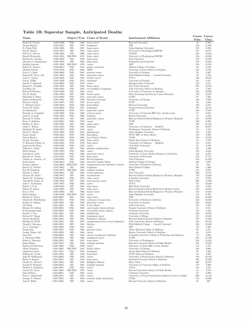
Table 1B: Superstar Sample, Anticipated DeathsName Cause of Death Institutional Affiliation

Career Pubs

Career Cites

Ernest G. Peralta (1959-1999) PhD 1986 brain cancer Harvard University 41 5,359George Khoury (1943-1987) MD 1970 lymphoma NIH 134 11,305B. Frank Polk (1942-1988) MD 1967 brain cancer Johns Hopkins University 107 8,226Joel D. Meyers (1944-1991) MD 1970 colon cancer University of Washington/FHCRC 171 14,717Melvin L. Marcus (1940-1989) MD 1966 colon cancer UMASS 225 15,034Harold Weintraub (1945-1995) MD/PhD 1973 brain cancer University of Washington/FHCRC 154 31,562Richard K. Gershon (1932-1983) MD 1959 lung cancer Yale University 182 12,007Theodore S. Zimmerman (1937-1988) MD 1963 lung cancer Scripps Research Institute 132 12,264Markku Linnoila (1947-1998) MD/PhD 1974 cancer NIH 513 21,254Robert F. Spencer (1949-2001) PhD 1974 gastric carcinoma Medical College of Virginia 59 2,136Michael Solursh (1942-1994) PhD 1968 AIDS University of Iowa School of Medicine 148 6,702Larry C. Clark (1948-2000) PhD 1981 prostate cancer University of Arizona 33 2,387Samuel W. Perry, 3rd (1941-1994) MD 1967 pancreatic cancer Weill Medical College — Cornell University 44 1,210Janis V. Giorgi (1947-2000) PhD 1977 uterine cancer UCLA 130 10,212Lois K. Miller (1945-1999) PhD 1972 melanoma University of Georgia 121 8,411Gerald T. Babcock (1946-2000) PhD 1973 cancer Michigan State University 123 8,511Edward C. Franklin (1928-1982) MD 1950 brain cancer New York University 224 12,761Tai-Shun Lin (1939-1994) PhD 1970 non hodgkin’s lymphoma Yale University School of Medicine 91 3,102Edwin H. Beachey (1934-1989) MD 1962 cancer University of Tennessee at Memphis 192 10,080Ora M. Rosen (1935-1990) MD 1960 breast cancer Sloan Kettering Institute for Cancer Research 150 14,587Elizabeth A. Bates (1974-2003) PhD 1974 pancreatic cancer UCSD 81 1,985Murray Rabinowitz (1927-1983) MD 1950 muscular dystrophy University of Chicago 146 8,229Helene S. Smith (1941-1997) PhD 1967 breast cancer UCSF 95 5,623C. Richard Taylor (1939-1995) PhD 1963 heart failure Harvard University 100 6,377Norton B. Gilula (1944-2000) PhD 1971 lymphoma Scripps Research Institute 99 13,147Ira Herskowitz (1946-2003) PhD 1971 pancreatic cancer UCSF 160 17,457Priscilla A. Campbell (1940-1998) PhD 1968 cervical cancer University of Colorado HSC/Nat. Jewish center 77 3,914Laird S. Cermak (1942-1999) PhD 1968 leukemia Boston University 73 2,338Bernard N. Fields (1938-1995) MD 1962 pancreatic cancer Harvard Medical School/Brigham & Women’s Hospital 181 10,505Peter A. Kollman (1944-2001) PhD 1970 cancer UCSF 189 9,095Wallace P. Rowe (1926-1983) MD 1948 colon cancer NIH 233 21,455Allan C. Wilson (1934-1991) PhD 1961 leukemia University of California — Berkeley 165 25,917Elizabeth M. Smith (1939-1997) PhD 1978 cancer Washington University School of Medicine 50 1,512David G. Marsh (1940-1998) PhD 1964 glioblastoma Johns Hopkins University 142 6,395Aaron Janoff (1930-1988) PhD 1959 long illness SUNY HSC at Stony Brook 131 8,590Nelson Butters (1937-1995) PhD 1964 Lou Gehrig’s disease UCSD 191 12,555George Némethy (1934-1994) PhD 1962 brain cancer Mount Sinai School of Medicine 76 7,079G. Harrison Echols, Jr. (1933-1993) PhD 1959 lung cancer University of California — Berkeley 113 9,191Lawrence H. Piette (1932-1992) PhD 1957 cancer Utah State University 61 2,766William L. Chick (1938-1998) MD 1963 diabetes complications UMASS 90 5,108Mette Strand (1937-1997) PhD 1964 cancer Johns Hopkins University 128 6,044Joachim G. Liehr (1942-2003) PhD 1968 pancreatic cancer University of Texas Medical Branch at Galveston 134 6,272Howard M. Temin (1934-1994) PhD 1959 lung cancer University of Wisconsin 212 17,277Charles A. Janeway, Jr. (1943-2003) MD 1969 B-cell lymphoma Yale University 313 31,455Keith Green (1940-2001) PhD 1964 died after lengthy illness Medical College of Georgia 206 2,572Gregory Mooser (1942-2003) DDS/PhD 1972 complications from alzheimer’s disease University of Southern California 23 962Harvey D. Preisler (1941-2002) MD 1965 lymphoma Rush Medical College 304 7,069Roy H. Steinberg (1935-1997) MD/PhD 1965 multiple myeloma UCSF 121 6,707Donald J. Cohen (1940-2001) MD 1966 ocular melanoma Yale University 299 12,177Thomas W. Smith (1936-1997) MD 1965 mesothelioma Harvard Medical School/Brigham & Women’s Hospital 170 12,826Marian W. Fischman (1939-2001) PhD 1972 colon cancer Columbia University 157 5,910Thoralf M. Sundt, Jr. (1930-1992) MD 1959 bone marrow cancer Mayo Clinic 208 11,099John C. Liebeskind (1935-1997) PhD 1962 cancer UCLA 147 10,160Robert J. Fass (1939-2002) MD 1964 lung cancer Ohio State University 132 3,703Sidney H. Ingbar (1925-1988) MD 1947 lung cancer Harvard Medical School/Beth Israel Medical Center 310 14,921Eva J. Neer (1937-2000) MD 1963 breast cancer Harvard Medical School/Brigham & Women’s Hospital 104 10,652Kiichi Sagawa (1926-1989) MD/PhD 1958 cancer Johns Hopkins University 119 9,491Richard J. Wyatt (1939-2002) MD 1964 lung cancer NIH 534 21,693Charles D. Heidelberger (1920-1983) PhD 1946 carcinoma of nasal sinus University of Southern California 243 19,260Sydney E. Salmon (1936-1999) MD 1962 pancreatic cancer University of Arizona 286 20,024Jiri Palek (1934-1998) MD 1958 2 year illness Tufts University 127 5,487Eleanor M. Saffran (1938-2002) PhD 1968 amyotrophic lateral sclerosis Temple University School of Medicine 41 2,811Irving Kupfermann (1938-2002) PhD 1964 Creutzfeldt-Jacob’s disease Columbia University 121 7,635Harold C. Neu (1934-1998) MD 1960 glioblastoma Columbia University 530 18,498Richard P. Bunge (1932-1996) MD 1960 esophageal cancer University of Miami 157 10,828Merton Bernfield (1938-2002) MD 1961 Parkinson’s Disease Harvard Medical School/Children’s Hospital 137 11,962Sheldon M. Wolff (1930-1994) MD 1957 complications from a renal malignancy Tufts University School of Medicine 224 22,128Gerald L. Klerman (1928-1992) MD 1954 diabetes Weill Medical College — Cornell University 253 19,458Leo J. Neuringer (1928-1993) PhD 1957 cancer MIT 39 1,264Frank Lilly (1930-1995) PhD 1965 prostate cancer Albert Einstein College of Medicine 95 4,471Joseph Stokes, 3rd (1924-1989) MD 1949 cancer Boston University School of Medicine 64 2,915Jane Pitt (1938-2003) MD 1964 chronic lymphocytic leukemia Columbia University College of Physicians and Surgeons 74 2,984J. Christian Gillin (1938-2003) MD 1966 esophageal cancer UCSD 355 15,729Edwin L. Bierman (1930-1995) MD 1955 bone cancer University of Washington 204 14,583Edgar Haber (1932-1997) MD 1956 multiple myeloma Harvard University School of Public Health 372 27,458Barbara H. Bowman (1930-1996) PhD 1959 cancer University of Texas HSC at San Antonio 115 3,371Albert Dorfman (1916-1982) MD/PhD 1944 kidney failure University of Chicago 183 9,660Charlotte Friend (1921-1987) PhD 1950 lymphoma Mount Sinai School of Medicine 98 5,486William H. Tooley (1925-1992) MD 1949 long illness UCSF School of Medicine 78 5,927John R. Williamson (1934-2000) PhD 1959 cancer University of Pennsylvania School of Medicine 210 16,530Henry S. Kaplan (1918-1984) MD 1940 lung cancer Stanford University School of Medicine 405 27,929Charles G. Moertel (1927-1994) MD 1953 Hodgkin’s Disease Mayo Clinic 302 22,557Joseph B. Warshaw (1936-2003) MD 1961 multiple myeloma University of Vermont College of Medicine 110 3,399Michael J. Goldstein (1930-1997) PhD 1957 cancer UCLA 118 4,221Gareth M. Green (1931-1998) MD/PhD 1957 cancer Harvard University School of Public Health 61 3,131John Gibbon (1934-2001) PhD 1967 cancer Columbia University 37 2,002Paul C. MacDonald (1930-1997) MD 1955 cancer University of Texas Southwestern Medical Center at Dallas 268 14,116George G. Glenner (1927-1995) MD 1953 systemic senile amyloidosis UCSD 152 15,369Jack E. White (1921-1988) MD 1944 cancer Howard University School of Medicine 35 282

Degree/Year

29

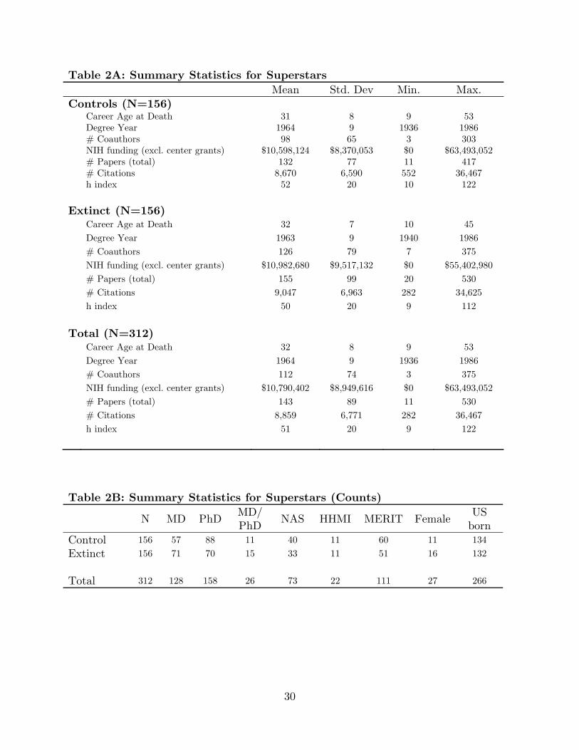
30

Table 2A: Summary Statistics for Superstars Mean Std. Dev Min. Max.Controls (N=156) Career Age at Death 31 8 9 53 Degree Year 1964 9 1936 1986 # Coauthors 98 65 3 303 NIH funding (excl. center grants) $10,598,124 $8,370,053 $0 $63,493,052 # Papers (total) 132 77 11 417 # Citations 8,670 6,590 552 36,467 h index 52 20 10 122

Extinct (N=156) Career Age at Death 32 7 10 45

Degree Year 1963 9 1940 1986

# Coauthors 126 79 7 375

NIH funding (excl. center grants) $10,982,680 $9,517,132 $0 $55,402,980

# Papers (total) 155 99 20 530

# Citations 9,047 6,963 282 34,625

h index 50 20 9 112

Total (N=312) Career Age at Death 32 8 9 53

Degree Year 1964 9 1936 1986

# Coauthors 112 74 3 375

NIH funding (excl. center grants) $10,790,402 $8,949,616 $0 $63,493,052

# Papers (total) 143 89 11 530

# Citations 8,859 6,771 282 36,467

h index 51 20 9 122

Table 2B: Summary Statistics for Superstars (Counts) N MD PhD MD/

PhD NAS HHMI MERIT Female US born

Control 156 57 88 11 40 11 60 11 134

Extinct 156 71 70 15 33 11 51 16 132

Total 312 128 158 26 73 22 111 27 266

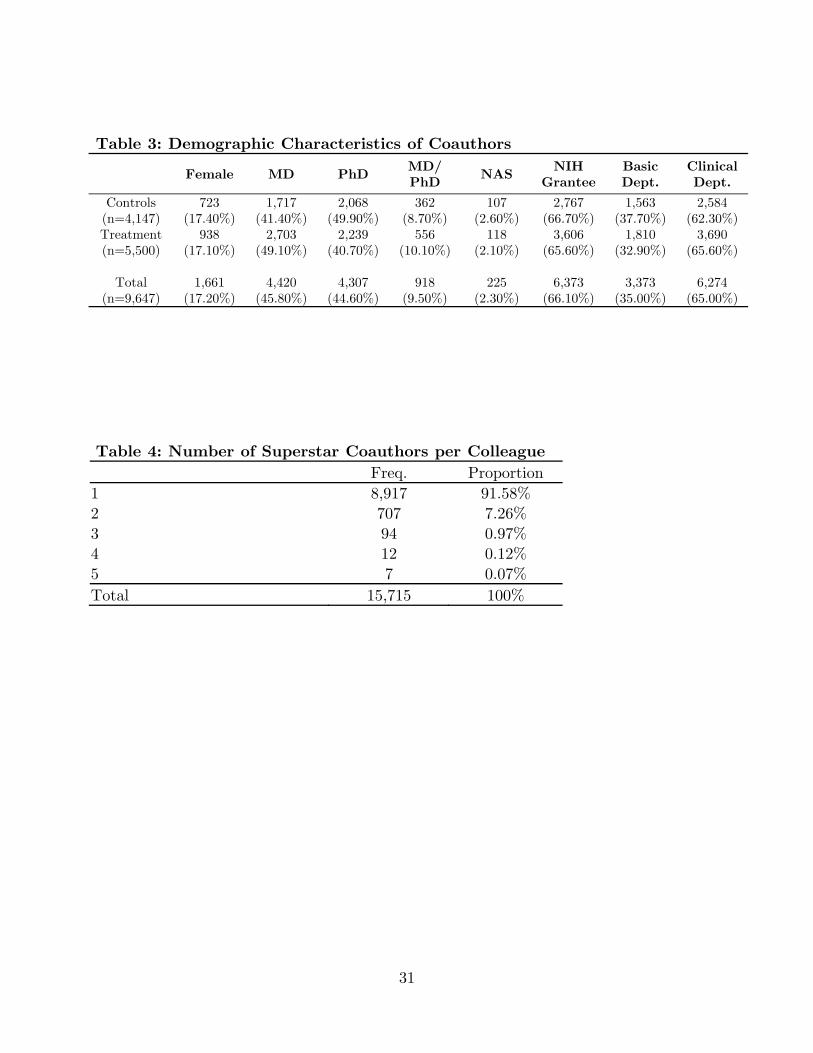
31

Table 3: Demographic Characteristics of Coauthors

Female MD PhD MD/ PhD NAS NIH

Grantee Basic Dept.

Clinical Dept.

Controls (n=4,147)

723 1,717 2,068 362 107 2,767 1,563 2,584 (17.40%) (41.40%) (49.90%) (8.70%) (2.60%) (66.70%) (37.70%) (62.30%)

Treatment (n=5,500)

938 2,703 2,239 556 118 3,606 1,810 3,690 (17.10%) (49.10%) (40.70%) (10.10%) (2.10%) (65.60%) (32.90%) (65.60%)

Total

(n=9,647) 1,661 4,420 4,307 918 225 6,373 3,373 6,274

(17.20%) (45.80%) (44.60%) (9.50%) (2.30%) (66.10%) (35.00%) (65.00%) Table 4: Number of Superstar Coauthors per Colleague

Freq. Proportion1 8,917 91.58%2 707 7.26%3 94 0.97%4 12 0.12%5 7 0.07%Total 15,715 100%

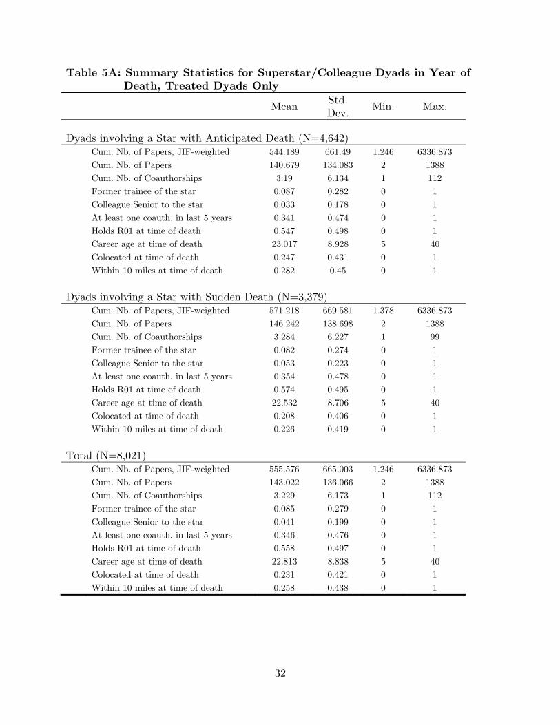
32

Table 5A: Summary Statistics for Superstar/Colleague Dyads in Year of Death, Treated Dyads Only

Mean Std. Dev.

Min. Max.

Dyads involving a Star with Anticipated Death (N=4,642) Cum. Nb. of Papers, JIF-weighted 544.189 661.49 1.246 6336.873

Cum. Nb. of Papers 140.679 134.083 2 1388

Cum. Nb. of Coauthorships 3.19 6.134 1 112

Former trainee of the star 0.087 0.282 0 1

Colleague Senior to the star 0.033 0.178 0 1

At least one coauth. in last 5 years 0.341 0.474 0 1

Holds R01 at time of death 0.547 0.498 0 1

Career age at time of death 23.017 8.928 5 40

Colocated at time of death 0.247 0.431 0 1

Within 10 miles at time of death 0.282 0.45 0 1

Dyads involving a Star with Sudden Death (N=3,379) Cum. Nb. of Papers, JIF-weighted 571.218 669.581 1.378 6336.873

Cum. Nb. of Papers 146.242 138.698 2 1388

Cum. Nb. of Coauthorships 3.284 6.227 1 99

Former trainee of the star 0.082 0.274 0 1

Colleague Senior to the star 0.053 0.223 0 1

At least one coauth. in last 5 years 0.354 0.478 0 1

Holds R01 at time of death 0.574 0.495 0 1

Career age at time of death 22.532 8.706 5 40

Colocated at time of death 0.208 0.406 0 1

Within 10 miles at time of death 0.226 0.419 0 1

Total (N=8,021) Cum. Nb. of Papers, JIF-weighted 555.576 665.003 1.246 6336.873

Cum. Nb. of Papers 143.022 136.066 2 1388

Cum. Nb. of Coauthorships 3.229 6.173 1 112

Former trainee of the star 0.085 0.279 0 1

Colleague Senior to the star 0.041 0.199 0 1

At least one coauth. in last 5 years 0.346 0.476 0 1

Holds R01 at time of death 0.558 0.497 0 1

Career age at time of death 22.813 8.838 5 40

Colocated at time of death 0.231 0.421 0 1

Within 10 miles at time of death 0.258 0.438 0 1

33

Table 5B: Summary Statistics for Superstar/Colleague Dyads in Year of

Death, Control vs. Treatment Dyads Mean Std. Dev Min. Max.Control Dyads (N=4,476) Career age at time of death 20.913 8.759 5 40 Time since first coauthorship 10.917 7.683 0 48 Number of Coauthorships in last 5 years 0.775 2.301 0 54 Cum. Nb. of Papers 67.363 66.077 1 765 Cum. Nb. of Papers, JIF-weighted 255.145 306.55 0.369 3490.446 Cum. Nb. of Patents 0.53 2.244 0 31 Cum. Nb. of Coauthorships 3.038 6.758 1 160 Holds R01 at time of death 0.541 0.498 0 1 Cum. NIH Funding at time of death $2,687,440 $4,664,128 $0 $54,236,564 School NIH Funding in year of death $180,085,816 $212,184,454 $0 $1,146,971,648 Proportion of Papers coauthored with star 0.104 0.163 0.001 1 Colocated at time of death 0.212 0.408 0 1 Within 10 miles at time of death 0.237 0.425 0 1 Former trainee of the star 0.123 0.329 0 1 Colleague Senior to the star 0.041 0.197 0 1 Treatment Dyads (N=6,220) Career age at time of death 22.086 8.816 5 40

Time since first coauthorship 11.147 7.774 0 39

Number of Coauthorships in last 5 years 0.803 2.192 0 40

Cum. Nb. of Papers 79.8 82.263 1 1071

Cum. Nb. of Papers, JIF-weighted 294.047 369.246 0.738 5019.836

Cum. Nb. of Patents 0.599 2.612 0 55

Cum. Nb. of Coauthorships 3.173 6.141 1 107

Holds R01 at time of death 0.515 0.5 0 1

Cum. NIH Funding at time of death $3,017,445 $6,168,175 $0 $123,224,432

School NIH Funding in year of death $177,066,269 $24,476,511 $0 $1,146,971,648

Proportion of Papers coauthored with star 0.095 0.158 0.001 1

Colocated at time of death 0.236 0.425 0 1

Within 10 miles at time of death 0.262 0.44 0 1

Former trainee of the star 0.095 0.293 0 1

Colleague Senior to the star 0.033 0.18 0 1

34

Table 6: Trends in Publication output in the years immediately preceding/following a

superstar’s death (1) (2) (3) (4)

156 Superstars, Age at death≤67

Excluding 89 whose death

was anticipated

Excluding 67 whose death was sudden

30 Superstars Age at death>75

156 Controls 67 Controls 89 Controls 30 Controls

2 years after year of death 0.311** 0.295** 0.315** 0.208** [6.36] [3.95] [5.26] [2.72]

1 year after year of death 0.697** 0.762 0.611** 1.237 [3.06] [1.36] [4.01] [0.52]

year of death 1.140 0.947 1.289† 0.728 [1.18] [0.30] [1.90] [0.92]

1 year before year of death 1.230* 1.067 1.333** 0.840 [2.25] [0.42] [2.58] [0.59]

2 years before year of death 1.038 0.905 1.118 1.087 [0.38] [0.65] [0.91] [0.29]

3 years before year of death 1.101 1.133 1.046 1.039 [1.02] [0.92] [0.38] [0.12]

4 years before year of death 1.150 0.968 1.302* 0.997 [1.49] [0.20] [2.41] [0.02]

Log Quasi-Likelihood -59,050 -24,095 -34,388 -11,393 Nb. of Observations 9,444 3,947 5,497 2,018 Nb. of Scientists 312 134 178 60 The estimates above are taken from a conditional fixed effects Poisson specification that also include 7 indicator variables corresponding to different age brackets and a full suite of calendar year effects (estimates not reported). The estimates are displayed as incidence rate ratios, e.g., the estimate in column (1) implies a statistically significant (1-0.311)=68.9% decrease in the rate of publication two years after a superstar scientist passes away (regardless of cause of death). Robust (QML) z-statistics are reported in brackets. The dependent variable is the weighted article count for the superstar, including only those publications in which the superstar appears in last position on the authorship list. The weights used to create these counts are Journal Impact Factors (JIF) published by the Institute for Scientific Information. †significant at 10%; *significant at 5%; **significant at 1%

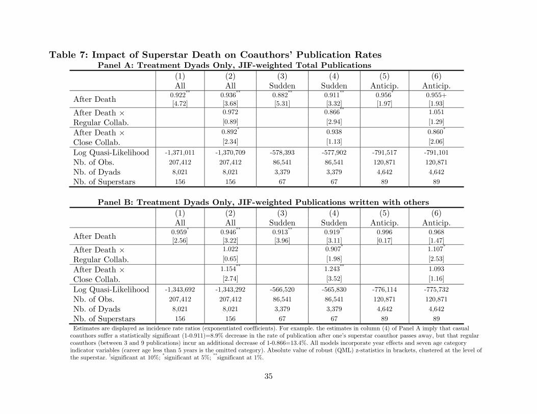
35

Table 7: Impact of Superstar Death on Coauthors’ Publication Rates Panel A: Treatment Dyads Only, JIF-weighted Total Publications

(1) (2) (3) (4) (5) (6) All All Sudden Sudden Anticip. Anticip.

After Death 0.922** 0.936** 0.882** 0.911** 0.956* 0.955+ [4.72] [3.68] [5.31] [3.32] [1.97] [1.93]

After Death × 0.972 0.866** 1.051

Regular Collab. [0.89] [2.94] [1.29]

After Death × 0.892* 0.938 0.860*

Close Collab. [2.34] [1.13] [2.06]

Log Quasi-Likelihood -1,371,011 -1,370,709 -578,393 -577,902 -791,517 -791,101

Nb. of Obs. 207,412 207,412 86,541 86,541 120,871 120,871

Nb. of Dyads 8,021 8,021 3,379 3,379 4,642 4,642

Nb. of Superstars 156 156 67 67 89 89

Panel B: Treatment Dyads Only, JIF-weighted Publications written with others

(1) (2) (3) (4) (5) (6) All All Sudden Sudden Anticip. Anticip.

After Death 0.959* 0.946** 0.913** 0.919** 0.996 0.968 [2.56] [3.22] [3.96] [3.11] [0.17] [1.47]

After Death × 1.022 0.907* 1.107*

Regular Collab. [0.65] [1.98] [2.53]

After Death × 1.154** 1.243** 1.093

Close Collab. [2.74] [3.52] [1.16]

Log Quasi-Likelihood -1,343,692 -1,343,292 -566,520 -565,830 -776,114 -775,732

Nb. of Obs. 207,412 207,412 86,541 86,541 120,871 120,871

Nb. of Dyads 8,021 8,021 3,379 3,379 4,642 4,642

Nb. of Superstars 156 156 67 67 89 89 Estimates are displayed as incidence rate ratios (exponentiated coefficients). For example. the estimates in column (4) of Panel A imply that casual coauthors suffer a statistically significant (1-0.911)=8.9% decrease in the rate of publication after one’s superstar coauthor passes away, but that regular coauthors (between 3 and 9 publications) incur an additional decrease of 1-0.866=13.4%. All models incorporate year effects and seven age category indicator variables (career age less than 5 years is the omitted category). Absolute value of robust (QML) z-statistics in brackets, clustered at the level of the superstar. †significant at 10%; *significant at 5%; **significant at 1%.

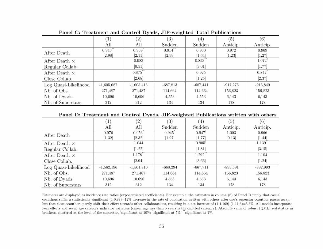
36

Panel C: Treatment and Control Dyads, JIF-weighted Total Publications (1) (2) (3) (4) (5) (6) All All Sudden Sudden Anticip. Anticip.

After Death 0.945** 0.959* 0.914** 0.950 0.972 0.969 [2.98] [2.11] [2.99] [1.64] [1.23] [1.27]

After Death × 0.983 0.853** 1.072†

Regular Collab. [0.51] [3.01] [1.77]

After Death × 0.875** 0.925 0.842*

Close Collab. [2.68] [1.25] [2.37]

Log Quasi-Likelihood -1,605,687 -1,605,415 -687,813 -687,441 -917,275 -916,849

Nb. of Obs. 271,487 271,487 114,664 114,664 156,823 156,823

Nb. of Dyads 10,696 10,696 4,553 4,553 6,143 6,143

Nb. of Superstars 312 312 134 134 178 178

Panel D: Treatment and Control Dyads, JIF-weighted Publications written with others

(1) (2) (3) (4) (5) (6) All All Sudden Sudden Anticip. Anticip.

After Death 0.976 0.956* 0.945* 0.947† 1.003 0.966 [1.32] [2.32] [1.97] [1.77] [0.13] [1.44]

After Death × 1.044 0.905† 1.139**

Regular Collab. [1.22] [1.81] [3.15]

After Death × 1.178** 1.292** 1.104

Close Collab. [2.94] [3.66] [1.24]

Log Quasi-Likelihood -1,562,196 -1,561,810 -668,294 -667,711 -893,391 -892,993

Nb. of Obs. 271,487 271,487 114,664 114,664 156,823 156,823

Nb. of Dyads 10,696 10,696 4,553 4,553 6,143 6,143

Nb. of Superstars 312 312 134 134 178 178 Estimates are displayed as incidence rate ratios (exponentiated coefficients). For example. the estimates in column (6) of Panel D imply that casual coauthors suffer a statistically significant (1-0.88)=12% decrease in the rate of publication written with others after one’s superstar coauthor passes away, but that close coauthors partly shift their effort towards other collaborations, resulting in a net increase of (1-1.169)-(1-11.6)=5.3%. All models incorporate year effects and seven age category indicator variables (career age less than 5 years is the omitted category). Absolute value of robust (QML) z-statistics in brackets, clustered at the level of the superstar. †significant at 10%; *significant at 5%; **significant at 1%.

37

Table 8: Ideas Spillovers Are Increasing in Superstar’s Accomplishments

Superstar’s Total Cites at Time of Death

Superstar’s Total Cites at Time of Death,

normalized by career length

Superstar’s Career NIH Funding

(1a) (1b) (2a) (2b) (3a) (3b)

w/o Controls with Controls w/o Controls with

Controls w/o

Controls with

Controls After Death × 1.007 1.034 1.012 1.040 0.899* 0.916*

Star in 1st Quartile [0.17] [0.79] [0.25] [0.85] [2.38] [2.00]

After Death × 0.949† 0.953 0.939* 0.948 0.936† 0.967

Star in 2nd Quartile [1.65] [1.39] [1.98] [1.35] [1.80] [0.77]

After Death × 0.895** 0.928* 0.918* 0.948 0.916** 0.945

Star in 3rd Quartile [3.38] [2.05] [2.55] [1.46] [2.67] [1.58]

After Death × 0.912** 0.936* 0.904** 0.927** 0.916** 0.948†

Star in 4th Quartile [3.68] [2.31] [4.14] [2.83] [3.15] [1.73]

Log Quasi-Likelihood -1,370,592 -1,605,491 -1,370,686 -1,605,483 -1,250,688 -1,507,523

Nb. of Obs. 207,412 271,487 207,412 271,487 189,821 256,027

Nb. of Dyads 8,021 10,696 8,021 10,696 7,360 10,108

Nb. of Superstars 156 312 156 312 146 296 Conditional dyad fixed effects quasi-MLE estimates for the determinants of JIF-weighted publications among coauthors of academic life sciences superstar academics. Estimates are displayed as incidence rate ratios (exponentiated coefficients). All models incorporate year effects and seven age category indicator variables (career age less than 5 years is the omitted category). Absolute value of robust (QML) z-statistics in brackets, clustered at the level of the superstar. We interact the treatment variable with 4 indicator variables corresponding to quartiles for four distinct metrics of achievement for the superstars at the time of their death: total citations, total citations normalized by years of career, and career NIH funding. In the latter case, we exclude 7 scientists who spend all their careers at NIH campus in Bethesda, MD, and are therefore not eligible to receive extramural NIH funding. †significant at 10%; *significant at 5%; **significant at 1%.

38

Table 9: Spillovers Are Not Increasing in Superstar’s Network Centrality

Betweenness Centrality Eigenvector Centrality Bonacich Centrality

(1a) (1b) (2a) (2b) (3a) (3b)

w/o Controlswith

Controls w/o Controls with

Controls w/o

Controls with

Controls After Death × 0.842* 0.815* 0.842* 0.815* 0.842* 0.815* Star in 1st Quartile [2.31] [2.44] [2.31] [2.44] [2.31] [2.44]

After Death × 0.971 0.867* 0.971 0.867* 0.971 0.867* Star in 2nd Quartile [0.66] [2.47] [0.66] [2.47] [0.66] [2.47]

After Death × 0.973 0.873** 0.973 0.873** 0.973 0.873** Star in 3rd Quartile [0.97] [3.68] [0.97] [3.68] [0.97] [3.68]

After Death × 0.910** 0.799** 0.910** 0.799** 0.910** 0.799** Star in 4th Quartile [4.11] [7.95] [4.11] [7.95] [4.11] [7.95]

Log Quasi-Likelihood -1,271,085 -2,440,786 -1,271,085 -2,440,786 -1,271,085 -2,440,786

Nb. of Obs. 191,046 426,306 191,046 426,306 191,046 426,306

Nb. of Dyads 7,392 17,944 7,392 17,944 7,392 17,944

Nb. of Superstars 137 369 137 369 137 369

Conditional dyad fixed effects quasi-MLE estimates for the determinants of JIF-weighted publications among coauthors of academic life sciences superstar academics. Estimates are displayed as incidence rate ratios (exponentiated coefficients). All models incorporate year effects and seven age category indicator variables (career age less than 5 years is the omitted category). Absolute value of robust (QML) z-statistics in brackets, clustered at the level of the superstar. We interact the treatment variable with 4 indicator variables corresponding to quartiles for four distinct measures of star centrality within the coauthorship network among 7,276 eminent life scientists. Because raw centrality measures are heavily correlated with publication output, the centrality measures on which the estimates are based are residuals from a simple regression of (raw) centrality on the stars’ stock of publications and a constant. †significant at 10%; *significant at 5%; **significant at 1%.

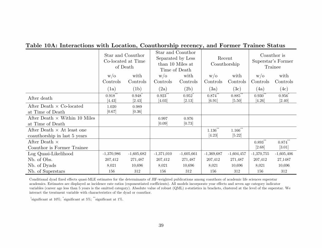
39

Table 10A: Interactions with Location, Coauthorship recency, and Former Trainee Status

Star and Coauthor Co-located at Time

of Death

Star and Coauthor Separated by Less than 10 Miles at Time of Death

Recent Coauthorship

Coauthor is Superstar’s Former

Trainee

w/o

Controls with

Controls w/o

Controls with

Controls w/o

Controls with

Controls w/o

Controlswith

Controls (1a) (1b) (2a) (2b) (3a) (3c) (4a) (4c)

After death 0.918** 0.948* 0.923** 0.952* 0.874** 0.885** 0.930** 0.956* [4.43] [2.43] [4.03] [2.13] [6.91] [5.50] [4.26] [2.40]

After Death × Co-located 1.020 0.989 at Time of Death [0.67] [0.36]

After Death × Within 10 Miles 0.997 0.976 at Time of Death [0.09] [0.73]

After Death × At least one 1.136** 1.166** coauthorship in last 5 years [4.23] [5.22]

After Death × 0.893** 0.874** Coauthor is Former Trainee [2.68] [3.01]

Log Quasi-Likelihood -1,370,986 -1,605,682 -1,371,010 -1,605,661 -1,369,687 -1,604,457 -1,370,755 -1,605,406

Nb. of Obs. 207,412 271,487 207,412 271,487 207,412 271,487 207,412 27,1487

Nb. of Dyads 8,021 10,696 8,021 10,696 8,021 10,696 8,021 10,696

Nb. of Superstars 156 312 156 312 156 312 156 312

Conditional dyad fixed effects quasi-MLE estimates for the determinants of JIF-weighted publications among coauthors of academic life sciences superstar academics. Estimates are displayed as incidence rate ratios (exponentiated coefficients). All models incorporate year effects and seven age category indicator variables (career age less than 5 years is the omitted category). Absolute value of robust (QML) z-statistics in brackets, clustered at the level of the superstar. We interact the treatment variable with characteristics of the dyad or coauthor.

†significant at 10%; *significant at 5%; **significant at 1%.

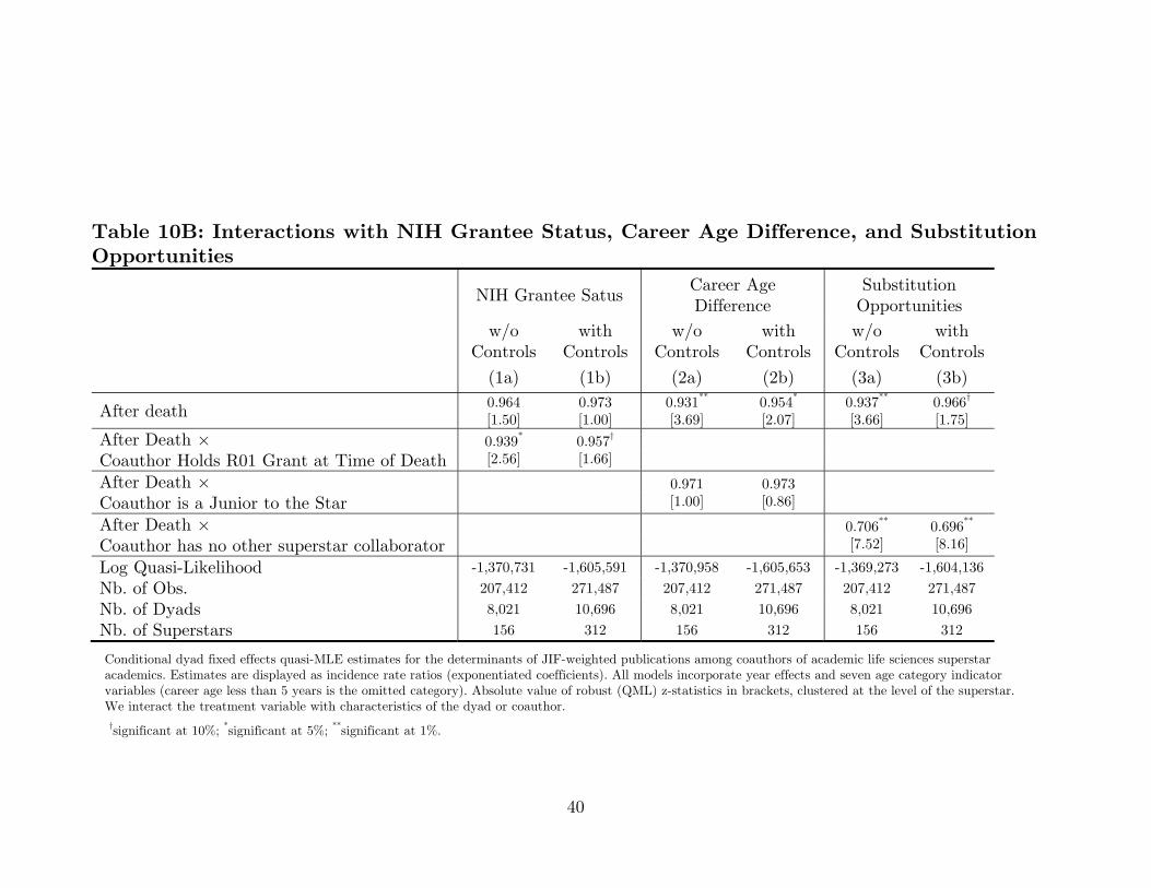
40

Table 10B: Interactions with NIH Grantee Status, Career Age Difference, and Substitution Opportunities

NIH Grantee Satus Career Age Difference

Substitution Opportunities

w/o

Controls with

Controls w/o

Controls with

Controls w/o

Controls with

Controls (1a) (1b) (2a) (2b) (3a) (3b)

After death 0.964 0.973 0.931** 0.954* 0.937** 0.966† [1.50] [1.00] [3.69] [2.07] [3.66] [1.75]

After Death × 0.939* 0.957† Coauthor Holds R01 Grant at Time of Death [2.56] [1.66]

After Death × 0.971 0.973 Coauthor is a Junior to the Star [1.00] [0.86]

After Death × 0.706** 0.696** Coauthor has no other superstar collaborator [7.52] [8.16]

Log Quasi-Likelihood -1,370,731 -1,605,591 -1,370,958 -1,605,653 -1,369,273 -1,604,136

Nb. of Obs. 207,412 271,487 207,412 271,487 207,412 271,487

Nb. of Dyads 8,021 10,696 8,021 10,696 8,021 10,696

Nb. of Superstars 156 312 156 312 156 312

Conditional dyad fixed effects quasi-MLE estimates for the determinants of JIF-weighted publications among coauthors of academic life sciences superstar academics. Estimates are displayed as incidence rate ratios (exponentiated coefficients). All models incorporate year effects and seven age category indicator variables (career age less than 5 years is the omitted category). Absolute value of robust (QML) z-statistics in brackets, clustered at the level of the superstar. We interact the treatment variable with characteristics of the dyad or coauthor.

†significant at 10%; *significant at 5%; **significant at 1%.

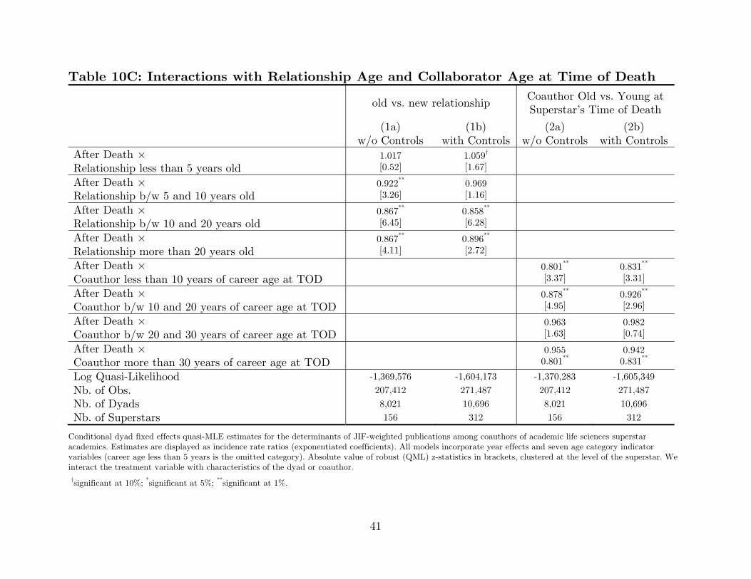
41

Table 10C: Interactions with Relationship Age and Collaborator Age at Time of Death

old vs. new relationship Coauthor Old vs. Young at Superstar’s Time of Death

(1a) (1b) (2a) (2b) w/o Controls with Controls w/o Controls with ControlsAfter Death × 1.017 1.059† Relationship less than 5 years old [0.52] [1.67]

After Death × 0.922** 0.969 Relationship b/w 5 and 10 years old [3.26] [1.16]

After Death × 0.867** 0.858** Relationship b/w 10 and 20 years old [6.45] [6.28]

After Death × 0.867** 0.896** Relationship more than 20 years old [4.11] [2.72]

After Death × 0.801** 0.831** Coauthor less than 10 years of career age at TOD [3.37] [3.31]

After Death × 0.878** 0.926** Coauthor b/w 10 and 20 years of career age at TOD [4.95] [2.96]

After Death × 0.963 0.982 Coauthor b/w 20 and 30 years of career age at TOD [1.63] [0.74]

After Death × 0.955 0.942 Coauthor more than 30 years of career age at TOD 0.801** 0.831**

Log Quasi-Likelihood -1,369,576 -1,604,173 -1,370,283 -1,605,349

Nb. of Obs. 207,412 271,487 207,412 271,487

Nb. of Dyads 8,021 10,696 8,021 10,696

Nb. of Superstars 156 312 156 312

Conditional dyad fixed effects quasi-MLE estimates for the determinants of JIF-weighted publications among coauthors of academic life sciences superstar academics. Estimates are displayed as incidence rate ratios (exponentiated coefficients). All models incorporate year effects and seven age category indicator variables (career age less than 5 years is the omitted category). Absolute value of robust (QML) z-statistics in brackets, clustered at the level of the superstar. We interact the treatment variable with characteristics of the dyad or coauthor.

†significant at 10%; *significant at 5%; **significant at 1%.

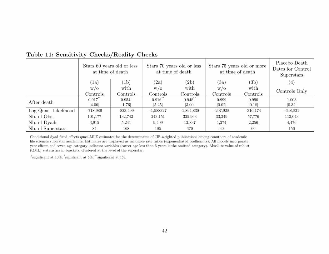
42

Table 11: Sensitivity Checks/Reality Checks

Stars 60 years old or less at time of death

Stars 70 years old or less at time of death

Stars 75 years old or more at time of death

Placebo Death Dates for Control

Superstars (1a) (1b) (2a) (2b) (3a) (3b) (4)

w/o

Controls with

Controls w/o

Controls with

Controls w/o

Controls with

Controls Controls Only

After death 0.917** 0.954† 0.916** 0.948** 0.999 0.990 1.003 [4.00] [1.76] [5.25] [3.00] [0.02] [0.18] [0.32]

Log Quasi-Likelihood -718,986 -823,499 -1,588327 -1,894,830 -207,928 -316,174 -648,821

Nb. of Obs. 101,177 132,742 243,151 325,963 33,349 57,776 113,043

Nb. of Dyads 3,915 5,241 9,409 12,837 1,274 2,256 4,476

Nb. of Superstars 84 168 185 370 30 60 156

Conditional dyad fixed effects quasi-MLE estimates for the determinants of JIF-weighted publications among coauthors of academic life sciences superstar academics. Estimates are displayed as incidence rate ratios (exponentiated coefficients). All models incorporate year effects and seven age category indicator variables (career age less than 5 years is the omitted category). Absolute value of robust (QML) z-statistics in brackets, clustered at the level of the superstar.

†significant at 10%; *significant at 5%; **significant at 1%.

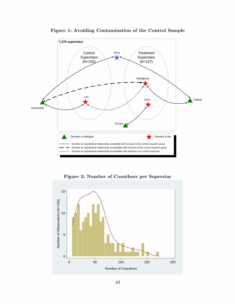
43

Figure 1: Avoiding Contamination of the Control Sample

7,276 superstars

TreatmentSuperstars

(N=137)

ControlSuperstars

(N=232)

Ganymede

Sirius

Betelgeuse

LeoCallistoOrion

Europa

Denotes a colleague Denotes a star

Denotes an hypothetical relationship compatible with inclusion in the control coauthor groupDenotes an hypothetical relationship incompatible with inclusion in the control coauthor groupDenotes an hypothetical relationship incompatible with selection as a control superstar

Figure 2: Number of Coauthors per Superstar

0

5

10

15

Num

ber o

f Obs

erva

tions

(N=1

56)

0 50 100 150 200

Number of Coauthors

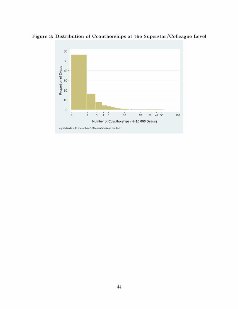
44

Figure 3: Distribution of Coauthorships at the Superstar/Colleague Level

0

10

20

30

40

50

60

Pro

porti

on o

f Dya

ds

1 2 3 4 5 10 20 30 40 50 100

Number of Coauthorships (N=10,696 Dyads) eight dyads with more than 100 coauthorships omitted

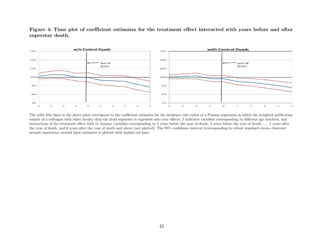
45

Figure 4: Time plot of coefficient estimates for the treatment effect interacted with years before and after superstar death.

The solid blue lines in the above plots correspond to the coefficient estimates for the incidence rate ratios of a Poisson regression in which the weighted publication output of a colleague with other faculty than the dead superstar is regressed onto year effects, 7 indicator variables corresponding to different age brackets, and interactions of the treatment effect with 11 dummy variables corresponding to 4 years before the year of death, 3 years before the year of death,…, 5 years after the year of death, and 6 years after the year of death and above (not plotted). The 95% confidence interval (corresponding to robust standard errors, clustered around supertsras) around these estimates is plotted with dashed red lines.