SUPER-CYCLES OF COMMODITYCYCLES OF COMMODITY … · SUPER-CYCLES OF COMMODITYCYCLES OF COMMODITY...

SUPER CYCLES OF COMMODITYSUPER-CYCLES OF COMMODITY PRICES SINCE THE MID-NINETEENTH

CENTURYCENTURY

José Antonio OcampoJosé Antonio OcampoProfessor, Columbia University

Presentation at the International Monetary FundMarch 20 2013March 20, 2013

Outline

1 I t d ti d R h Obj ti1. Introduction and Research Objectives

2. Brief Literature Review

3. Data Sources

4. Identification of Super-Cycles and Empirical4. Identification of Super Cycles and Empirical Results

5. Relationship between Commodity Prices and5. Relationship between Commodity Prices and Global Output: Short- and Long-term

6. Conclusions and Policy Implications6. Conclusions and Policy Implications

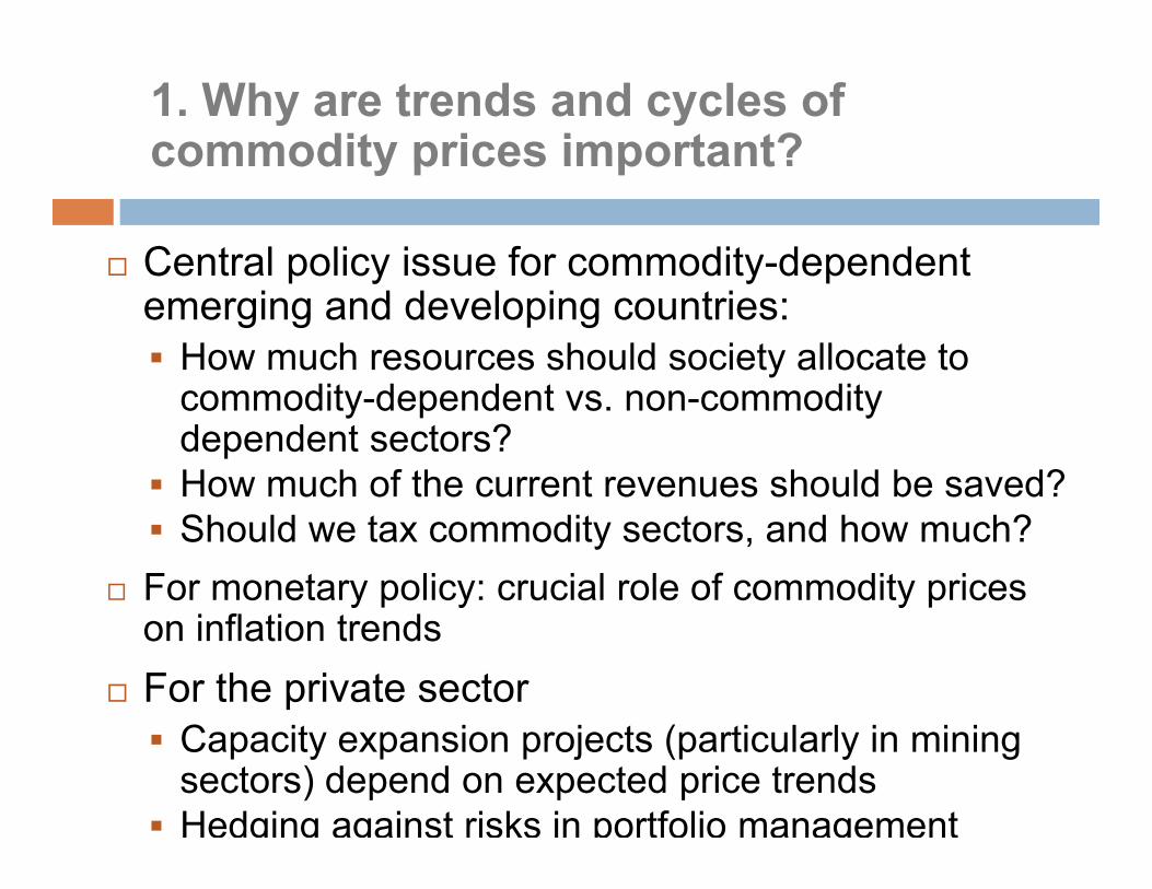
1. Why are trends and cycles of commodity prices important?commodity prices important?

Central policy issue for commodity-dependent p y y pemerging and developing countries: How much resources should society allocate to

dit d d t ditcommodity-dependent vs. non-commodity dependent sectors?

How much of the current revenues should be saved? Should we tax commodity sectors, and how much?

For monetary policy: crucial role of commodity prices on inflation trends

For the private sectorC i i j ( i l l i i i Capacity expansion projects (particularly in mining sectors) depend on expected price trends

Hedging against risks in portfolio management

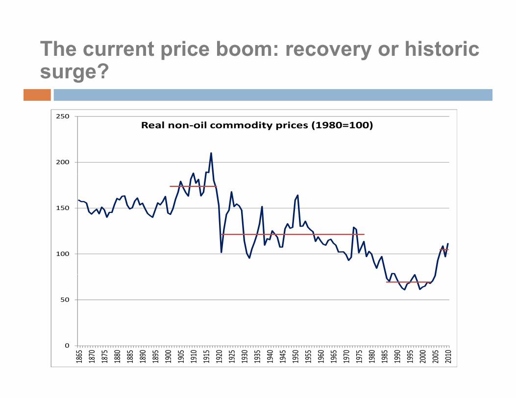
The current price boom: recovery or historic surge?surge?

250

Real non oil commodity prices (1980 100)

200

Real non-oil commodity prices (1980=100)

150

100

50

0

1865

1870

1875

1880

1885

1890

1895

1900

1905

1910

1915

1920

1925

1930

1935

1940

1945

1950

1955

1960

1965

1970

1975

1980

1985

1990

1995

2000

2005

2010

Research Objectives

Separate long-term trends from medium and p gshort-term cycles: Do commodity prices exhibit any long-term

d d d t d ? A thupward or downward trends? Are there differences across different groups of commodities, and why?

Should changes be described as structural breaks or super-cycles?Are the super cycle components in different Are the super-cycle components in different groups highly correlated, as would be expected if the super-cycle is demand-driven?

After separating the long-term trends and super-cycles, how strong are the shorter cycles?

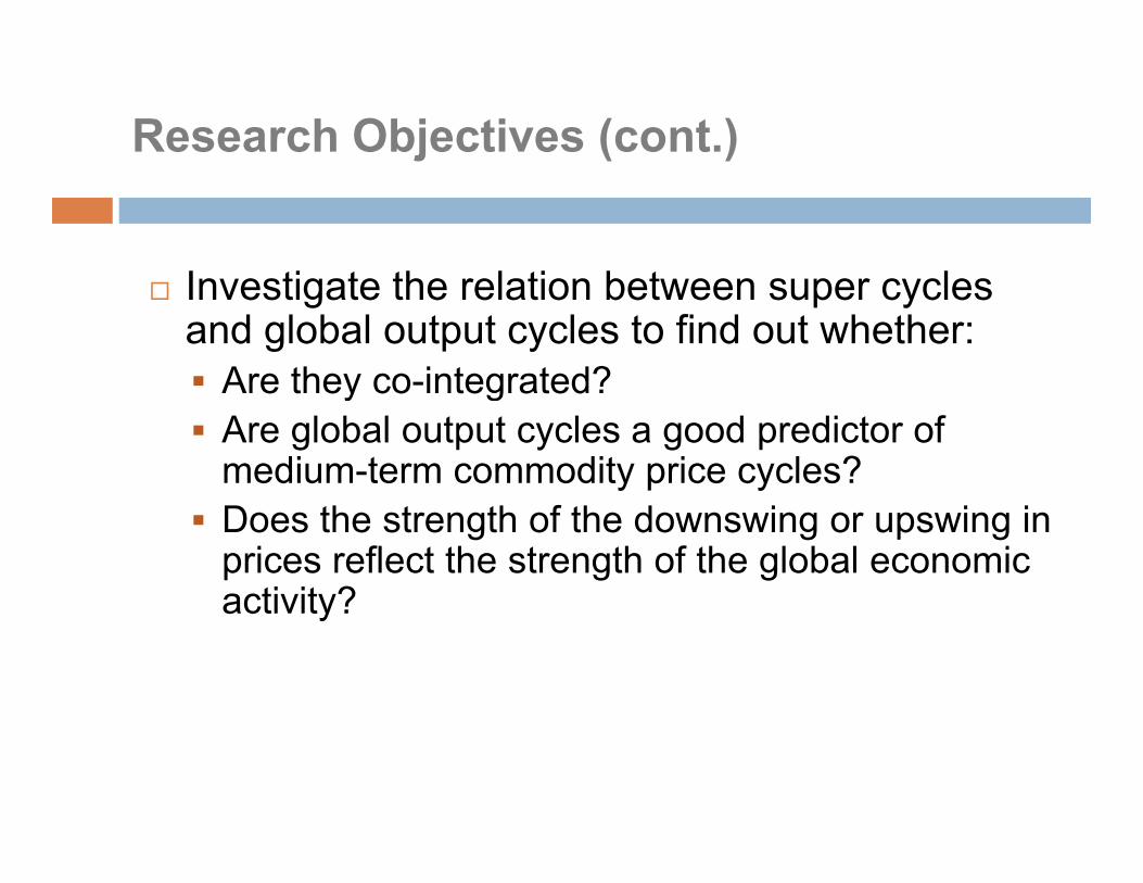
Research Objectives (cont.)

I ti t th l ti b t l Investigate the relation between super cycles and global output cycles to find out whether: Are they co-integrated?Are they co integrated? Are global output cycles a good predictor of

medium-term commodity price cycles? Does the strength of the downswing or upswing in

prices reflect the strength of the global economic activity?activity?

2. Literature Review

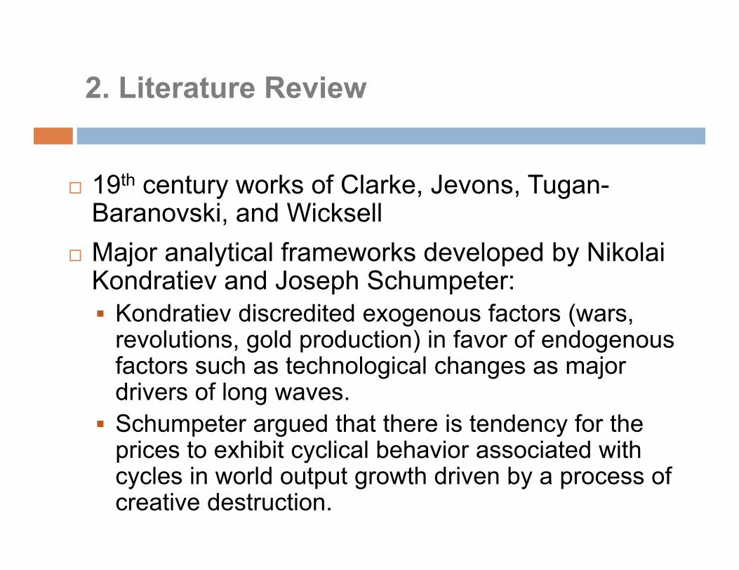
19th t k f Cl k J T 19th century works of Clarke, Jevons, Tugan-Baranovski, and WicksellMajor analytical frameworks developed by Nikolai Major analytical frameworks developed by Nikolai Kondratiev and Joseph Schumpeter: Kondratiev discredited exogenous factors (wars,Kondratiev discredited exogenous factors (wars,

revolutions, gold production) in favor of endogenous factors such as technological changes as major drivers of long wavesdrivers of long waves.

Schumpeter argued that there is tendency for the prices to exhibit cyclical behavior associated with cycles in world output growth driven by a process of creative destruction.

Literature Review (cont.)( )

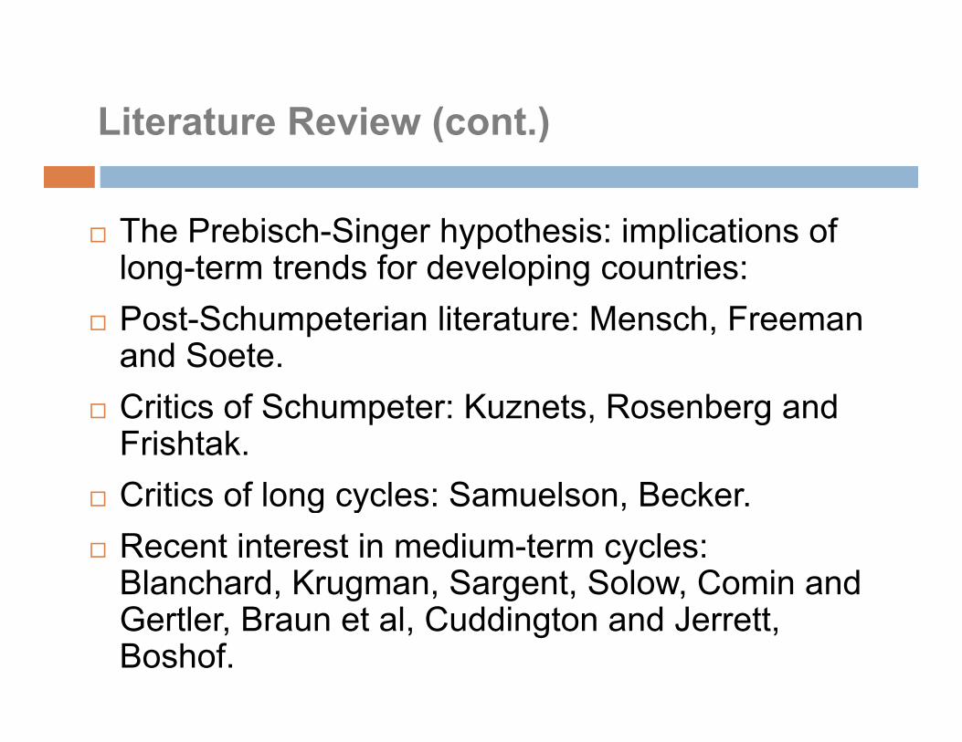
The Prebisch Singer hypothesis: implications of The Prebisch-Singer hypothesis: implications of long-term trends for developing countries:

Post-Schumpeterian literature: Mensch Freeman Post Schumpeterian literature: Mensch, Freeman and Soete.

Critics of Schumpeter: Kuznets, Rosenberg and Critics of Schumpeter: Kuznets, Rosenberg and Frishtak.

Critics of long cycles: Samuelson, Becker.g y Recent interest in medium-term cycles:

Blanchard, Krugman, Sargent, Solow, Comin and Gertler, Braun et al, Cuddington and Jerrett,Boshof.

3. Data sources

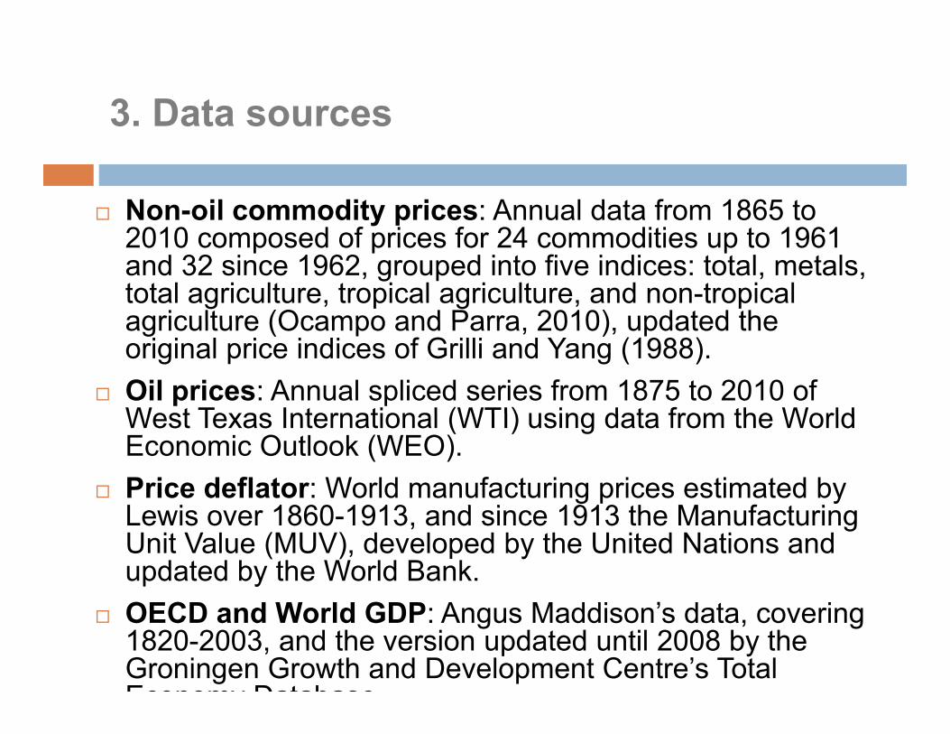
Non-oil commodity prices: Annual data from 1865 to 2010 d f i f 24 diti t 19612010 composed of prices for 24 commodities up to 1961 and 32 since 1962, grouped into five indices: total, metals, total agriculture, tropical agriculture, and non-tropical agriculture (Ocampo and Parra 2010) updated theagriculture (Ocampo and Parra, 2010), updated the original price indices of Grilli and Yang (1988).

Oil prices: Annual spliced series from 1875 to 2010 of West Texas International (WTI) using data from the WorldWest Texas International (WTI) using data from the World Economic Outlook (WEO).

Price deflator: World manufacturing prices estimated by L i 1860 1913 d i 1913 th M f t iLewis over 1860-1913, and since 1913 the Manufacturing Unit Value (MUV), developed by the United Nations and updated by the World Bank.

OECD and World GDP: Angus Maddison’s data, covering 1820-2003, and the version updated until 2008 by the Groningen Growth and Development Centre’s Total Economy Database

4. Identification of super-cycles

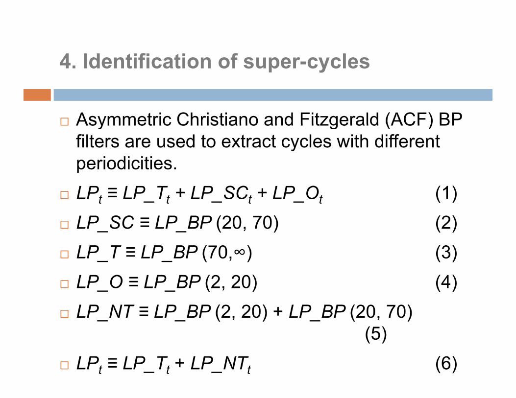
Asymmetric Christiano and Fitzgerald (ACF) BP Asymmetric Christiano and Fitzgerald (ACF) BP filters are used to extract cycles with different periodicities.

LPt ≡ LP_Tt + LP_SCt + LP_Ot (1) LP SC ≡ LP BP (20 70) (2) LP_SC ≡ LP_BP (20, 70) (2) LP_T ≡ LP_BP (70,∞) (3) LP_O ≡ LP_BP (2, 20) (4) LP_NT ≡ LP_BP (2, 20) + LP_BP (20, 70)

(5) LPt ≡ LP_Tt + LP_NTt (6)

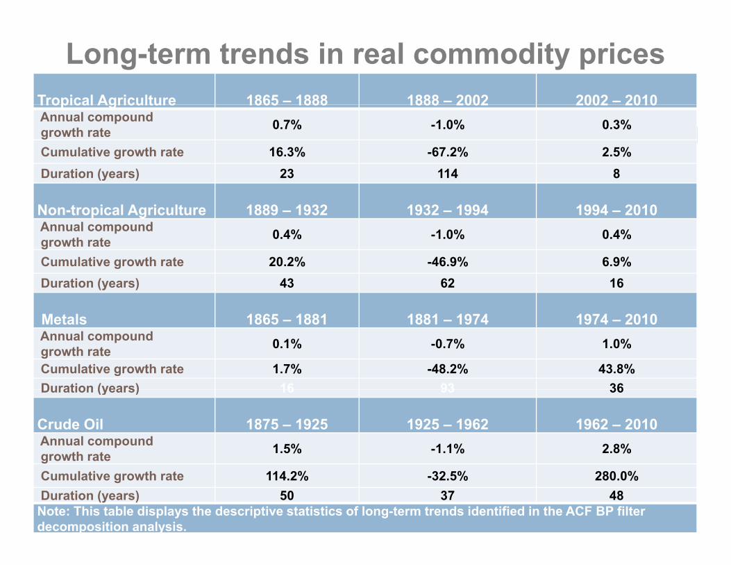
Long-term trends in real commodity pricesTropical Agriculture 1865 – 1888 1888 – 2002 2002 – 2010Tropical Agriculture 1865 1888 1888 2002 2002 2010 Annual compoundgrowth rate 0.7% -1.0% 0.3%

Cumulative growth rate 16.3% -67.2% 2.5%Duration (years) 23 114 8Duration (years) 23 114 8

Non-tropical Agriculture 1889 – 1932 1932 – 1994 1994 – 2010 Annual compoundgrowth rate 0.4% -1.0% 0.4%gCumulative growth rate 20.2% -46.9% 6.9%Duration (years) 43 62 16

Metals 1865 1881 1881 1974 1974 2010Metals 1865 – 1881 1881 – 1974 1974 – 2010 Annual compoundgrowth rate 0.1% -0.7% 1.0%

Cumulative growth rate 1.7% -48.2% 43.8%Duration (years) 16 93 36Duration (years) 16 93 36

Crude Oil 1875 – 1925 1925 – 1962 1962 – 2010 Annual compoundgrowth rate 1.5% -1.1% 2.8%g o t ateCumulative growth rate 114.2% -32.5% 280.0%Duration (years) 50 37 48Note: This table displays the descriptive statistics of long-term trends identified in the ACF BP filter decomposition analysis.

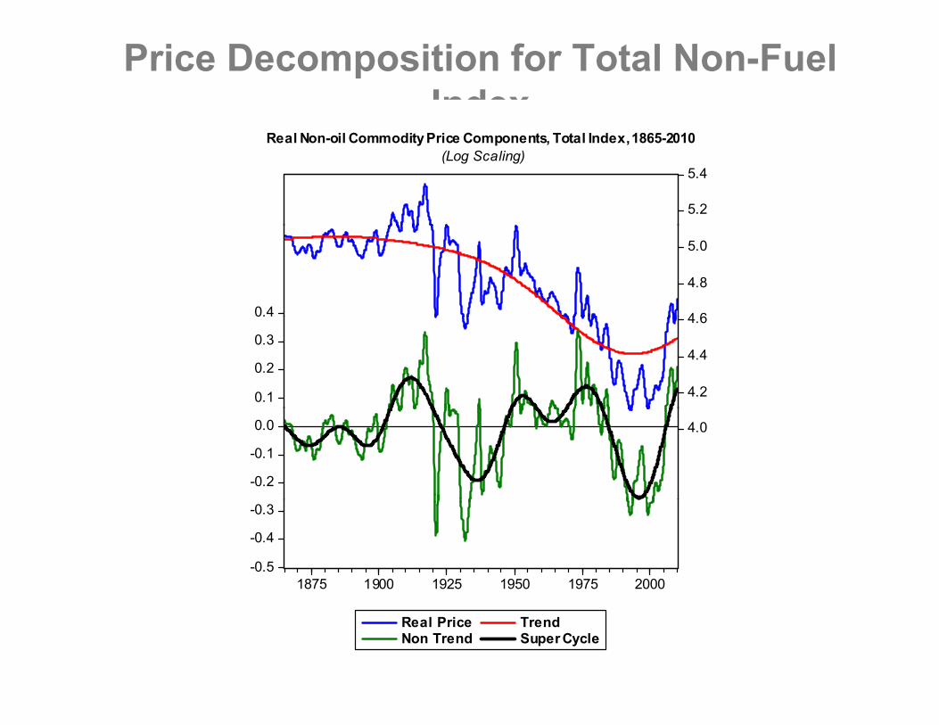
Price Decomposition for Total Non-Fuel Index

R l N il C dit P i C t T t l I d 1865 2010

5.2

5.4

Real Non-oil CommodityPrice Components, Total Index,1865-2010(Log Scaling)

0.4 4 6

4.8

5.0

0.1

0.2

0.3

4.2

4.4

4.6

-0.2

-0.1

0.0 4.0

-0.5

-0.4

-0.3

1875 1900 1925 1950 1975 2000

Real Price TrendNon Trend Super Cycle

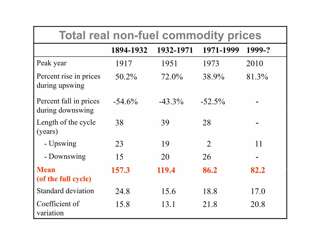
Total real non-fuel commodity prices1894-1932 1932-1971 1971-1999 1999-?

Peak year 1917 1951 1973 2010Percent rise in prices 50 2% 72 0% 38 9% 81 3%Percent rise in prices during upswing

50.2% 72.0% 38.9% 81.3%

Percent fall in prices -54.6% -43.3% -52.5% -during downswingLength of the cycle (years)

38 39 28 -

˗ Upswing 23 19 2 11˗ Downswing 15 20 26 -

Mean 157 3 119 4 86 2 82 2Mean (of the full cycle)

157.3 119.4 86.2 82.2

Standard deviation 24.8 15.6 18.8 17.0Coefficient of variation

15.8 13.1 21.8 20.8

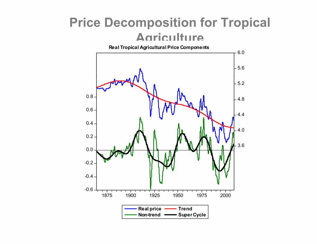
Price Decomposition for Tropical Agriculture

5.6

6.0Real Tropical Agricultural Price Components

0.8 4.8

5.2

0 2

0.4

0.6

4.0

4.4

-0.2

0.0

0.2

3.6

-0.6

-0.4

1875 1900 1925 1950 1975 2000

Real price TrendNon-trend Super Cycle

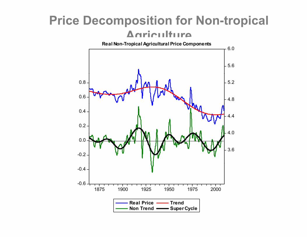
Price Decomposition for Non-tropical Agriculture

Real Non Tropical Agricultural Price Components

5.6

6.0Real Non-Tropical Agricultural Price Components

0.6

0.8

4.8

5.2

0.2

0.4

4 0

4.4

-0.2

0.0

3.6

4.0

-0.6

-0.4

1875 1900 1925 1950 1975 2000


Price Decomposition for Metals

5.6

6.0Real Metal Price Components

0 6

0.84.8

5.2

0.2

0.4

0.6

4.0

4.4

-0.2

0.0 3.6

-0.6

-0.4

1875 1900 1925 1950 1975 2000


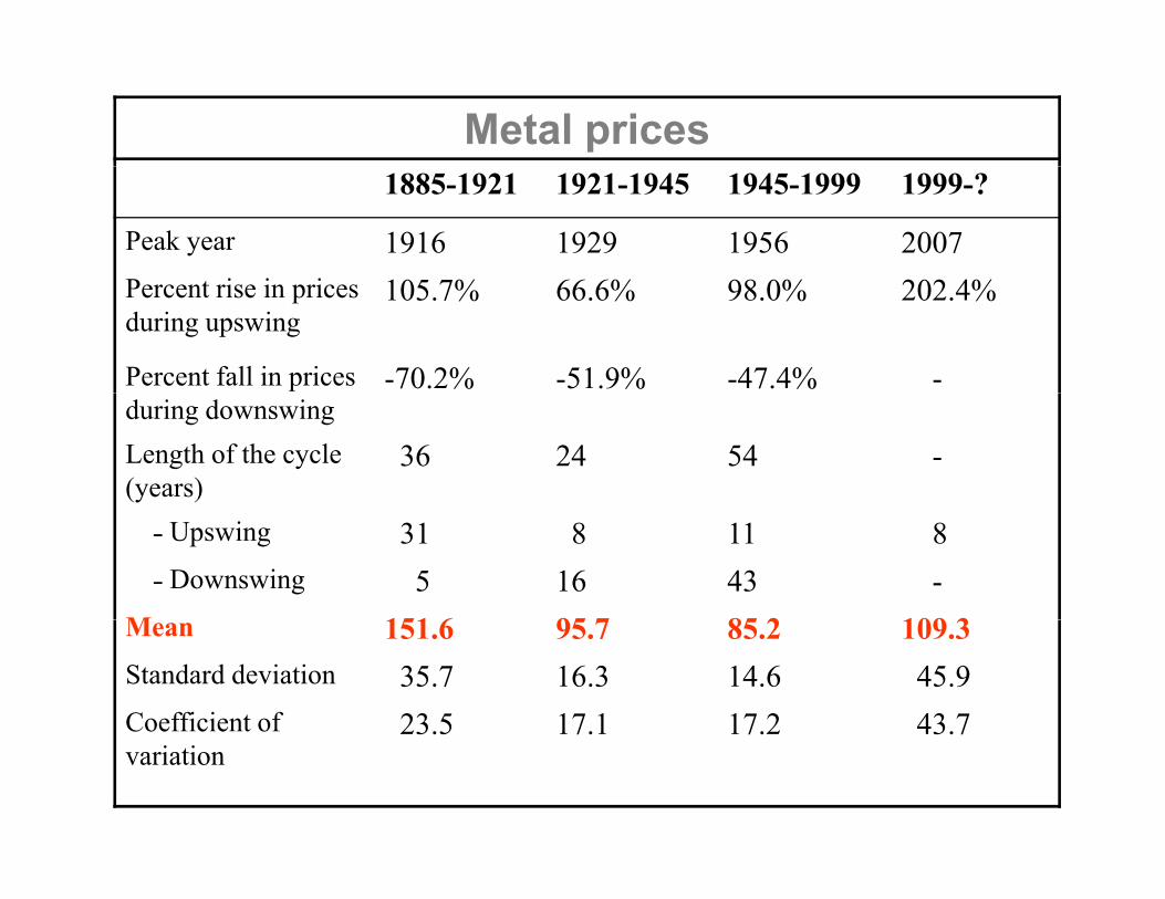
Metal prices1885-1921 1921-1945 1945-1999 1999-?

Peak year 1916 1929 1956 2007P i i i 10 % 66 6% 98 0% 202 4%Percent rise in prices during upswing

105.7% 66.6% 98.0% 202.4%


36 24 54 -


M 151 6 95 7 85 2 109 3Mean 151.6 95.7 85.2 109.3Standard deviation 35.7 16.3 14.6 45.9Coefficient of 23.5 17.1 17.2 43.7variation

23.5 17.1 17.2 43.7

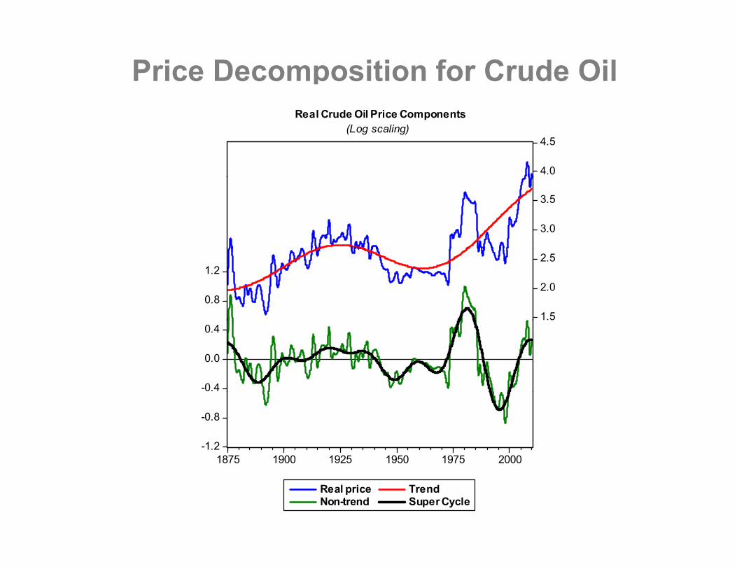
Price Decomposition for Crude Oil

4.0

4.5

Real Crude Oil Price Components(Log scaling)

3.0

3.5

0.8

1.2

1.5

2.0

2.5

-0.4

0.0

0.4

-1.2

-0.8

1875 1900 1925 1950 1975 2000

Real price TrendNon-trend Super Cycle

Crude oil pricesp1892-1947 1947-1973 1973-1998 1998-?

Peak year 1920 1958 1980 2008Percent rise in prices during upswing

402.8% 27.4% 363.2% 466.5%


55 26 25 -


M 36 9 24 8 53 2 91 2Mean 36.9 24.8 53.2 91.2Standard deviation 3.9 0.7 8.5 16.4Coefficient of variation 27.9 7.5 42.0 47.4

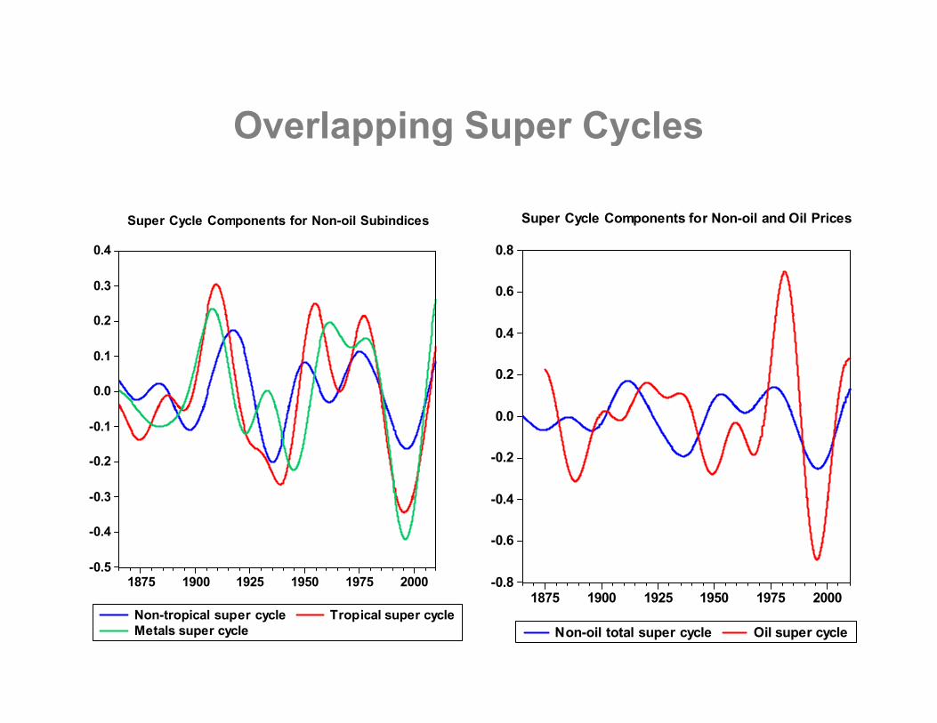
Overlapping Super CyclesOverlapping Super Cycles

Super Cycle Components for Non-oil Subindices Super Cycle Components for Non-oil and Oil Prices

0 2

0.3

0.4

Super Cycle Components for Non oil Subindices

0.6

0.8

p y p

0.0

0.1

0.2

0.2

0.4

-0 3

-0.2

-0.1

0 4

-0.2

0.0

-0.5

-0.4

-0.3

1875 1900 1925 1950 1975 2000 -0.8

-0.6

-0.4

Non-tropical super cycle Tropical super cycleMetals super cycle

1875 1900 1925 1950 1975 2000

Non-oil total super cycle Oil super cycle

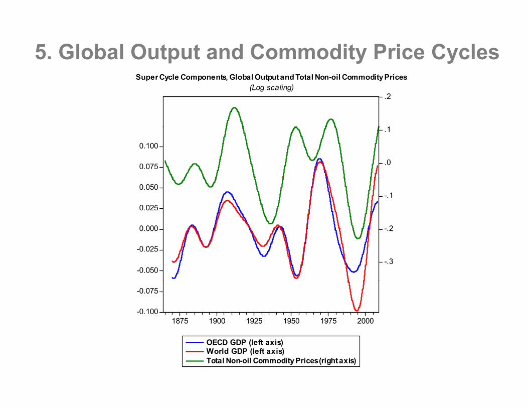
5. Global Output and Commodity Price CyclesS C l C t Gl b l O t t d T t l N il C dit P i

1

.2

Super Cycle Components, Global Outputand Total Non-oil Commodity Prices(Log scaling)

0.075

0.100

.0

.1

0 000

0.025

0.050

- 2

-.1

-0.050

-0.025

0.000

-.3

.2

-0.100

-0.075

1875 1900 1925 1950 1975 2000

OECD GDP (left axis)World GDP (left axis)Total Non-oil Commodity Prices (right axis)

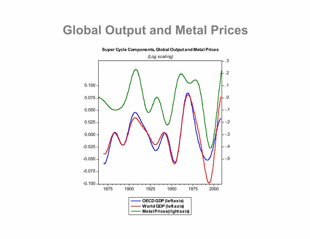
Global Output and Metal Prices

.2

.3

Super Cycle Components, Global Output and Metal Prices(Log scaling)

0.075

0.100

.0

.1

0 000

0.025

0.050

- 3

-.2

-.1

-0.050

-0.025

0.000

-.5

-.4

-.3

-0.100

-0.075

1875 1900 1925 1950 1975 2000

OECD GDP (left axis)World GDP (left axis)Metal Prices (right axis)

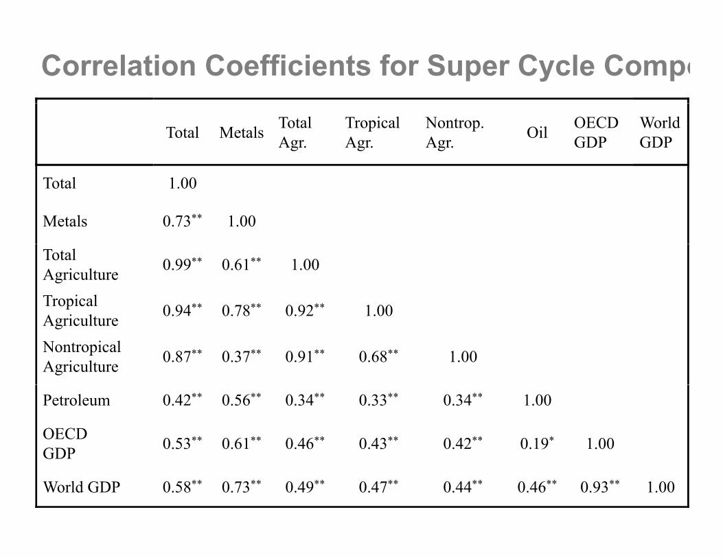
Correlation Coefficients for Super Cycle Compo

Total Metals Total Agr.

TropicalAgr.

Nontrop.Agr. Oil OECD

GDPWorldGDP

Total 1.00

Metals 0.73** 1.00

TotalAgriculture 0.99** 0.61** 1.00

Tropicali l 0.94** 0.78** 0.92** 1.00Agriculture 0.94 0.78 0.92 1.00

NontropicalAgriculture 0.87** 0.37** 0.91** 0.68** 1.00

Petroleum 0.42** 0.56** 0.34** 0.33** 0.34** 1.00

OECDGDP 0.53** 0.61** 0.46** 0.43** 0.42** 0.19* 1.00GDP

World GDP 0.58** 0.73** 0.49** 0.47** 0.44** 0.46** 0.93** 1.00

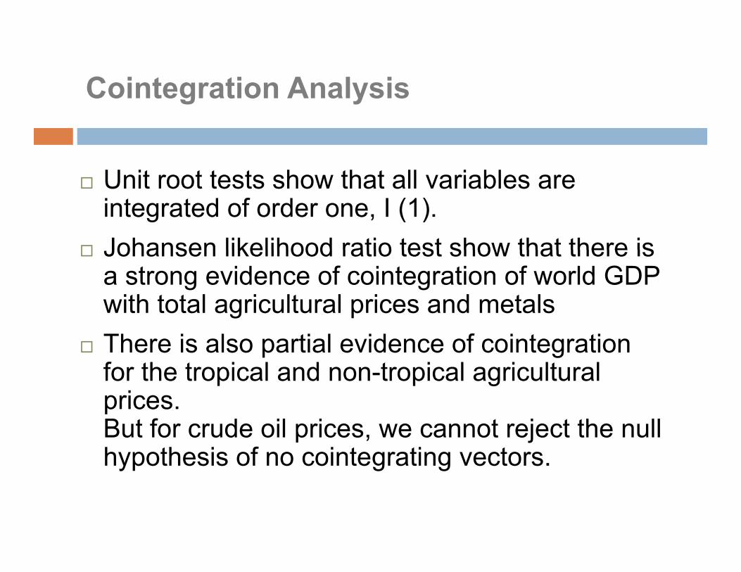
Cointegration Analysis

Unit root tests show that all variables are Unit root tests show that all variables are integrated of order one, I (1).

Johansen likelihood ratio test show that there is Johansen likelihood ratio test show that there is a strong evidence of cointegration of world GDP with total agricultural prices and metals

There is also partial evidence of cointegrationfor the tropical and non-tropical agricultural

iprices.But for crude oil prices, we cannot reject the null hypothesis of no cointegrating vectors.yp g g

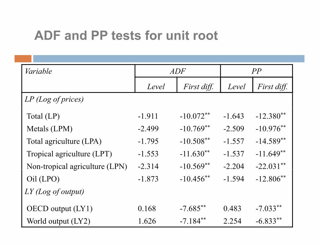
ADF and PP tests for unit root

Variable ADF PP

Level First diff. Level First diff.LP (Log of prices)

Total (LP) -1.911 -10.072** -1.643 -12.380**

Metals (LPM) -2.499 -10.769** -2.509 -10.976**

T l i l (LPA) 1 795 10 508** 1 557 14 589**Total agriculture (LPA) -1.795 -10.508** -1.557 -14.589**

Tropical agriculture (LPT) -1.553 -11.630** -1.537 -11.649**

Non-tropical agriculture (LPN) -2.314 -10.569** -2.204 -22.031**p g ( )Oil (LPO) -1.873 -10.456** -1.594 -12.806**

LY (Log of output)

OECD output (LY1) 0.168 -7.685** 0.483 -7.033**

World output (LY2) 1.626 -7.184** 2.254 -6.833**

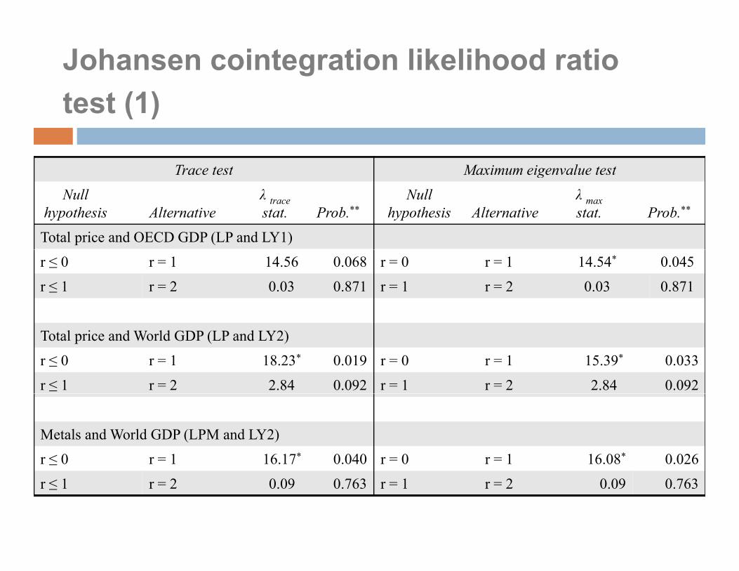
Johansen cointegration likelihood ratio test (1)test (1)

Trace test Maximum eigenvalue testg

Null hypothesis Alternative

λ tracestat. Prob.**


λ maxstat. Prob.**

Total price and OECD GDP (LP and LY1)

r ≤ 0 r = 1 14.56 0.068 r = 0 r = 1 14.54* 0.045

r ≤ 1 r = 2 0.03 0.871 r = 1 r = 2 0.03 0.871

Total price and World GDP (LP and LY2)

r ≤ 0 r = 1 18.23* 0.019 r = 0 r = 1 15.39* 0.033

r ≤ 1 r = 2 2.84 0.092 r = 1 r = 2 2.84 0.092

Metals and World GDP (LPM and LY2)

r ≤ 0 r = 1 16.17* 0.040 r = 0 r = 1 16.08* 0.026

r ≤ 1 r = 2 0.09 0.763 r = 1 r = 2 0.09 0.763

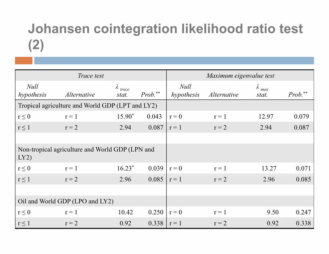
Johansen cointegration likelihood ratio test (2)(2)

Trace test Maximum eigenvalue testg


λ tracestat. Prob.**


λ maxstat. Prob.**

Tropical agriculture and World GDP (LPT and LY2)

r ≤ 0 r = 1 15.90* 0.043 r = 0 r = 1 12.97 0.079

r ≤ 1 r = 2 2.94 0.087 r = 1 r = 2 2.94 0.087

Non-tropical agriculture and World GDP (LPN and LY2)

r ≤ 0 r = 1 16.23* 0.039 r = 0 r = 1 13.27 0.071

r ≤ 1 r = 2 2.96 0.085 r = 1 r = 2 2.96 0.085

Oil and World GDP (LPO and LY2)

r ≤ 0 r = 1 10.42 0.250 r = 0 r = 1 9.50 0.247

r ≤ 1 r = 2 0.92 0.338 r = 1 r = 2 0.92 0.338

Analysis of error correction models

The coefficients of the error correction terms The coefficients of the error correction terms indicate unidirectional causality that runs from global output to non-fuel commodity prices without any feedback effect in the long run implying thatany feedback effect in the long-run – implying that world GDP is a useful predictor of non-fuel prices in LR.

The error correction term for metals shows that the real metal prices change by 26% in the first year following a deviation from long run equilibrium Thisfollowing a deviation from long-run equilibrium. This speed of adjustment is the highest compared to other adjustment rates, implying that the metal

i ti l l iti t h iprices are particularly sensitive to changes in economic activity in the LR.

There is also a short-run relationship running from

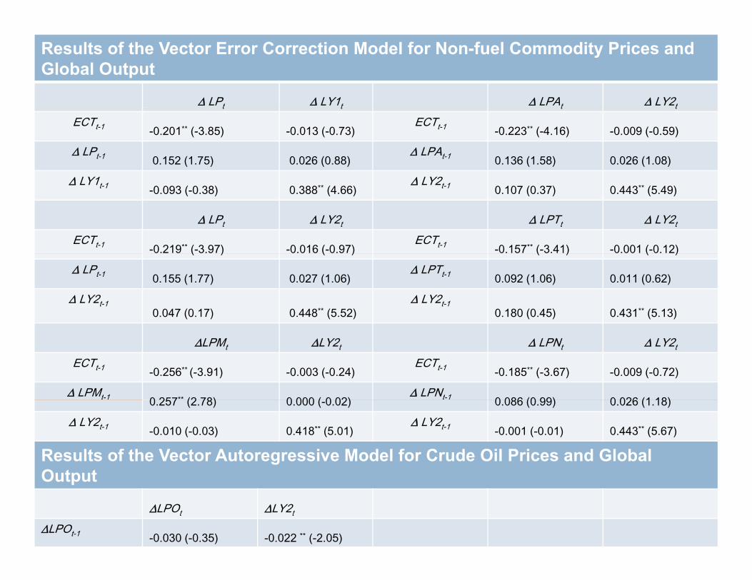
Results of the Vector Error Correction Model for Non-fuel Commodity Prices and Global Output

∆ LPt ∆ LY1t ∆ LPAt ∆ LY2tt t t t

ECTt-1 -0.201** (-3.85) -0.013 (-0.73)ECTt-1 -0.223** (-4.16) -0.009 (-0.59)

∆ LPt-1 0.152 (1.75) 0.026 (0.88)∆ LPAt-1 0.136 (1.58) 0.026 (1.08)

∆ LY1 ∆ LY2∆ LY1t-1 -0.093 (-0.38) 0.388** (4.66)∆ LY2t-1 0.107 (0.37) 0.443** (5.49)

∆ LPt ∆ LY2t ∆ LPTt ∆ LY2t

ECTt-1 -0.219** (-3.97) -0.016 (-0.97)ECTt-1 -0.157** (-3.41) -0.001 (-0.12)( ) ( ) ( ) ( )

∆ LPt-1 0.155 (1.77) 0.027 (1.06)∆ LPTt-1 0.092 (1.06) 0.011 (0.62)

∆ LY2t-10.047 (0.17) 0.448** (5.52)

∆ LY2t-10.180 (0.45) 0.431** (5.13)

∆LPMt ∆LY2t ∆ LPNt ∆ LY2t

ECTt-1 -0.256** (-3.91) -0.003 (-0.24)ECTt-1 -0.185** (-3.67) -0.009 (-0.72)

∆ LPMt-1 0 257** (2 78) 0 000 ( 0 02)∆ LPNt-1 0 086 (0 99) 0 026 (1 18)0.257 (2.78) 0.000 (-0.02) 0.086 (0.99) 0.026 (1.18)

∆ LY2t-1 -0.010 (-0.03) 0.418** (5.01)∆ LY2t-1 -0.001 (-0.01) 0.443** (5.67)

Results of the Vector Autoregressive Model for Crude Oil Prices and Global OutputOutput

∆LPOt ∆LY2t

∆LPOt-1 -0.030 (-0.35) -0.022 ** (-2.05)

6. Conclusions and Policy Implications

A major characteristic of commodity prices is 30-40 year-long l hi h t d t l i ifi tl bsuper-cycles, which tend to overlap significantly across sub-

indices (including oil since the 1950s). The amplitudes vary between 20-40 percent from long-run p y p g

trend: tropical agriculture exhibits super-cycles with greater amplitude relative to non-tropical agriculture.

The mean of each super cycle for non fuel commodities has The mean of each super-cycle for non-fuel commodities has a tendency to be lower than that of the previous cycle, suggesting a step-wise deterioration over the entire period.

Tropical agriculture experienced a severe long-term downward trend through most of the twentieth century, followed by non-tropical agriculture and metals.

Real oil prices experienced a long-term upward trend, which was only interrupted during some four decades of the twentieth century

Conclusions and Policy Implications (cont.)

Since world economic activity is a strong predictor of dit i th i dit i bcommodity prices, the ongoing commodity price boom

could last only if China and other major developing countries are capable of delinking from slow growth

t d i d l d t iexpected in developed countries. Commodity-dependent countries should be aware of

price cycles, and develop policies to take advantage ofprice cycles, and develop policies to take advantage of the expansionary phases while taking precautionary action against the contraction phases.

Step wise deterioration underlines the importance of Step-wise deterioration underlines the importance of diversification.

Supply-side factors associated with resource depletion may have become an additional drivers of prices.

Investments in commodity futures have also become an important determinant of short-term fluctuations in

SUPER CYCLES OF COMMODITYSUPER-CYCLES OF COMMODITY PRICES SINCE THE MID-NINETEENTH

CENTURYCENTURY

José Antonio OcampoJosé Antonio OcampoProfessor, Columbia University

Presentation at the International Monetary FundMarch 20 2013March 20, 2013

SUPER-CYCLES OF COMMODITYCYCLES OF COMMODITY … · SUPER-CYCLES OF COMMODITYCYCLES OF COMMODITY...

Documents

Transcript of SUPER-CYCLES OF COMMODITYCYCLES OF COMMODITY … · SUPER-CYCLES OF COMMODITYCYCLES OF COMMODITY...