Subsalt imaging for exploration, production, and ... Center/Technical... · Subsalt imaging for...

Subsalt imaging for exploration, production, and development: A review

Jacques P. Leveille1, Ian F. Jones2, Zheng-Zheng Zhou2, Bin Wang3, and Faqi Liu4

ABSTRACT

The field of subsalt imaging has evolved rapidly in the lastdecade, thanks in part to the availability of low cost massivecomputing infrastructure, and also to the development of newseismic acquisition techniques that try to mitigate the problemscaused by the presence of salt. This paper serves as an introduc-tion to the special Geophysics section on Subsalt Imaging forE&P. The purpose of the special section is to bring togetherpractitioners of subsalt imaging in the wider sense, i.e., not onlyalgorithm developers, but also the interpretation community thatutilizes the latest technology to carry out subsalt exploration anddevelopment. The purpose of the paper is in many ways peda-gogical and historical. We address the question of what subsaltimaging is and discuss the physics of the subsalt imaging pro-blem, especially the illumination issue. After a discussion of theproblem, we then give a review of the main algorithms that havebeen developed and implemented within the last decade, namelyKirchhoff and Beam imaging, one-way wavefield extrapolation

methods and the full two-way reverse time migration. This re-view is not meant to be exhaustive, and is qualitative to make itaccessible to a wide audience. For each method and algorithmwe highlight the benefits and the weaknesses. We then addressthe imaging conditions that are a fundamental part of each ima-ging algorithm. While we dive into more technical detail, thesection should still be accessible to a wide audience. Gathersof various sorts are introduced and their usage explained. Modelbuilding and velocity update strategies and tools are presentednext. Finally, the last section shows a few results from specificalgorithms. The latest techniques such as waveform inversion orthe “dirty salt” techniques will not be covered, as they will beelaborated upon by other authors in the special section. With themassive effort that the industry has devoted to this field, muchremains to be done to give interpreters the accurate detailedimages of the subsurface that are needed. In that sense the saltis still winning, although the next decade will most likelychange this situation.

INTRODUCTION

Energy companies are constantly pushing into different andusually more challenging environments in the search for hydrocar-bons worldwide. For quite a while now, salt basins worldwide havebeen one of the places to find the most prospective hydrocarbonreserves. The best-known salt basins are probably in the Gulf ofMexico, where recent activity has led to a large number of discov-eries, and the salt basins of the West African Margin, such asAngola and Gabon, which have been well explored and prolific.Recently, the subsalt basins of the Brazilian margins have seengigantic discoveries such as Tupi, where billions of barrels of oilin place have been discovered.

Salt basins, especially tertiary basins with mobilized salt, arenotoriously difficult places to explore because of the traditionallypoor subsurface images typically obtained around and below salt.In this paper, we review the geophysical reasons for these difficul-ties in imaging and the steady progress that has been made. Thesereasons will, in general, be different depending on the details of thesalt and on the geological history of the basins, but reasonable gen-eralizations can be made.The difficulties encountered by everyone in the industry in the

past prompted various groups to start working together to try andsolve these difficult imaging problems. In 2005, a special two dayworkshop was organized at the Colorado School of Mines, with avery different purpose: The organizers asked everyone to bring only

Manuscript received by the Editor 1 May 2011; revised manuscript received 3 June 2011; published online 22 November 2011.1ION Geophysical, Houston, Texas, USA, E-mail: [email protected]/ GX Technology, Houston, Texas, USA, E-mail: [email protected]; [email protected] NOPEC, Houston, Texas, USA., E-mail: [email protected] Corporation, Houston, Texas, USA, E-mail: [email protected].

© 2011 Society of Exploration Geophysicists. All rights reserved.

WB3

GEOPHYSICS. VOL. 76, NO. 5 (SEPTEMBER-OCTOBER 2011); P. WB3–WB20, 16 FIGS.10.1190/GEO2011-0156.1

Downloaded 24 Nov 2011 to 217.20.19.226. Redistribution subject to SEG license or copyright; see Terms of Use at http://segdl.org/

problems related to subsalt imaging, not solutions. The idea was tolay all the problems on the table, with the hope that exposing theseproblems would spur on ideas, especially in academic circles, andaccelerate the pace of research in this subject. In the 17 talks pre-sented in that workshop, gloom was apparent in every corner, withdifficulties encountered above salt, near salt, and subsalt. The baseof salt was disappearing without good explanations, and the subsaltimages were less than clear. (Leveille et al., 2005). This led PaulSinger of then Total to ask his often repeated question: “Is the saltwinning?” Although the answer in 2005 was probably yes, a fan-tastic amount of new techniques have been developed since thattime, and it looks very much as if the E&P industry is on the vergeof winning, although much more progress will be needed to fullyhelp in the drilling of subsalt prospects which remain to this day acostly and risky enterprise. While most of the progress originallycame through new seismic acquisition techniques, such as wide-azimuth surveys, rich-azimuth surveys, and a resulting alphabetsoup of specialized wide azimuth acquisitions, imaging throughthe incorporation of better physics came in the form of reverse timemigration (RTM) with full anisotropy. In this review, we will notreview in any detail the recently developed acquisition techniquesthemselves, but rather refer the reader to the existing literature(see e.g. Corcoran et al., 2007; Howard and Moldoveanu 2006;Moldoveanu et al., 2008). Instead, we will highlight the problemsthat necessitated these new techniques and what the new resultsbased on these techniques look like.In this review, we attempt to summarize the wide-ranging field

of subsalt imaging, and the progress that has been made since theearly days. These will take the form of new seismic acquisition tech-niques and of imaging and computing techniques. The whole sub-field of subsalt velocity updating has exploded and has benefittedfrom these computing advances. The progress in the technology hasbeen chronicled in a succession of successful workshops heldaround the globe by the SEG and the EAGE.The computational revolution that has been going on over the last

decade has allowed for the new imaging techniques to blossom, andmuch more is expected in the next decade. It seems that we are onlylimited by our imagination rather than compute cycles. However,not every subsalt problem has been solved, and many challengesremain. We will spend a little time discussing these remainingissues.

THE PHYSICS OF SUBSALT IMAGING

Subsalt Imaging is actually a misnomer, which has been derivedfrom the problems encountered in trying to image around andbelow allochtonous salt sheets in the Gulf of Mexico. The problemis trying to image below a fast velocity medium, such as salt,encased in an acoustically slow material such as tertiary sedimentsin the Gulf of Mexico. Similar issues will be encountered imagingthrough and around basalt encased in softer sediments. Before weget into the details of the difficulty encountered, it might be usefulto review a few basic properties of salt tectonics.Salt is a ubiquitous rock in many basins worldwide. Salt origin-

ally deposited in ancient times, such as the Jurassic Period in theGulf of Mexico, and still in its original emplacement is called auto-chtonous. Usually, the acoustic impedance contrast between auto-chtonous salt and its encasing rocks is not very great, usually around10% or less. In such cases, imaging through the autochtonous saltcauses no serious problems and can be handled with a variety of

simple imaging algorithms, such as Kirchhoff techniques. That isthe case for the Lou-Ann Jurassic salt in the Gulf of Mexico, stillencased in Jurassic and older Cretaceous rocks. A similar situationis encountered in the North Sea with in-place Zechstein salt. In fact,that is mostly the situation as well for the recent discoveries inBrazil.Salt is mechanically a very weak rock, and when stress is applied

to it, salt can flow if given an appropriate weak conduit. It is oftensaid that salt behaves just like toothpaste in that it flows whensqueezed, but only if some opening/conduit exists, and like tooth-paste it is mechanically unable to support large shear stresses.Therefore, salt does not “punch” through sediments, but ratherflows along preexisting weak points if available. When salt “flows”it usually rises toward the surface, overriding sediments, and endsup forming large canopies of salt with much younger sediments sur-rounding it. These displaced salt bodies, not in their originalemplacement of deposition, are called allochtonous and are the saltsheets that are often seen in younger tertiary basins such as the Gulfof Mexico, the West Africa basins, and many more.The allochtonous canopies are usually formed by various epi-

sodes of salt movement. These episodes can result in very thick saltsheets, with thicknesses from a few hundred to three to five thou-sand meters or so. When the salt moves, it can entrain sedimentswith it. These sediments can be overridden by more salt, and even-tually get trapped within the salt sheet. Salt sheets that “flow” canalso collide and amalgamate into what looks like a larger salt sheet.Usually, sediments are trapped between the colliding salt sheets,forming what are called sutures. It is not unusual to have severalsutures within what looks like a large continuous salt body.The net result is that allochtonous salt sheets can vary in com-

position, from more or less pure salt, to what is now referred to as“dirty” salt containing trapped sediments called inclusions. Theseinclusions can vary in size from a few meters to tens of meters.Incidentally, these dirty salt inclusions are well known to salt mineengineers who detect them routinely near the edges of salt mines.These trapped sediments are usually shale material, which has beencaught up as the salt moves near the surface. The trapped sedimentsare usually undrained sediments, and when they are encased, thewater has no place to drain. As more salt or sediments are depositedover the salt, these “inclusions” become more pressurized. Theseinclusions can be overpressured, therefore having very low veloci-ties, and can cause serious drilling hazards.The composition of the material trapped in the sutures can vary

widely. If the sediments are much younger, they will usually havethe same properties as the inclusions discussed above. However, thesediments can also be age equivalent to the original salt, and there-fore be much older, more compacted rocks. This makes suturesrather difficult to quantify a priori from a seismic velocity pointof view and is still a very difficult problem.What do we expect at the top of salt? Geologically, the salt is

overriding sediments and this usually occurs near the sea floor.As such, the sediments deposited over the salt will tend to beyounger than the salt. The age difference depends on the details ofthe timing of the salt movement. For the problem at hand, we willassume that the sediments are much younger, either Pliocene orPleistocene. Therefore, the sediments overlying the salt will beacoustically much less compacted, and there will be a great varia-tion in the acoustic velocities between the salt and the sediments.We will cover this in more detail below. Another thing that is

WB4 Leveille et al.


expected, is that the top of the salt will not be uniform. In fact, weshould expect the top salt surface to be very rugose. This topsalt rugosity is well known and follows from basic salt tectonicsprinciples (see for example Hudec and Jackson, 2007).In other instances, possibly large blocks of sediments can ride on

top of the moving salt. These are called “rafts” or “rafted sequences,”although the newest term used to describe these sediments is “car-apaces.”These carapaces can consist of varying lithologies, althoughthe most common are shales and carbonates. Because these rafts areolder sediments, their seismic velocities can be quite high, and theycan be quite dense. These carapaces are not very thick, although theirthickness can reach several hundreds of meters. We will not discussthese rafts any further in this review, but the practitioner of subsaltimaging must always be vigilant and consult a friendly structuralgeologist as to the possibility of rafts in a specific situation.The expectation for the base salt is different. Since the salt is

“overriding” existing sediments, starting from some feeder pointconnected to the deep “mother salt,” we expect that the base of saltsurface will be reasonably smooth and flat, as deposited sedimentsare. Although there is variability in the base salt surface, it is indeedmuch smoother than the top. In fact, rapid variations in the base saltshape are more than likely associated with either the “feeder” con-nection to the salt sheet, with the suturing of two or more saltbodies, or with later faulting. Geologists will look closely at thediscontinuity of the base of salt to detect and unravel these features.Indeed, somewhere under the salt, either near the edges toward thesalt wall or anywhere under the canopy will be at least one salt fee-der system. These feeders provide very useful information to thegeologists trying to reconstruct the history of the basin. Unfortu-nately, the feeders are still difficult to image and they are usuallyvery steeply dipping. Finally, what do we expect subsalt in terms ofsediments? The answer is just about anything. The subsalt sedi-ments will be age equivalent to the salt movement, so the age ofthe sediment abutting the base salt will depend on the time at whichsalt started to move. This leads to an interesting and complex geo-logical problem: Depending on how many salt sheets formed thesalt mass, there could be rapid variability in the age of the sedimentssubsalt. One salt sheet overriding Miocene sediments could easilycollide with a salt sheet overriding Cretaceous sediments, with a netresult of a deep Miocene subsalt basin separated from a deep cre-taceous basin subsalt by some salt feeder that may or may not con-tain remnants of salt. This basin juxtaposition can form very goodtraps for hydrocarbons.There is no limit to the number of salt sheets in principle.

Although in practice, it is very rare to find more than one or twoallochtonous salt sheets. Imaging through a single salt sheet isalready very complex and the problem becomes increasingly moredifficult with additional salt.So the physical picture that one should carry for the remainder

of this review, is that of a reasonably thick salt sheet (of order of1–5 km), with a rugose top (with possibly rapid variations), and areasonably flat base with several possibly sharp discontinuities. Thesediments at the top of the salt sheet are usually much younger thanthe salt, while the subsalt sediments can really be of any age. Theflank of the salt sheet will usually be very steep, although greatvariability can occur. This sets up the geophysical problem.Pure salt geophysical properties are as follows: compressional

velocity of 4500 m/s, a VP∕VS ratio of 1.9 and a density of2.16 grams∕cm3. In this review, we will not focus on elastic issues,

so we will more or less ignore the shear velocity. Almost all currentimaging algorithms are acoustic in nature, and most of these algo-rithms assume a constant density. Salt is extremely light, but veryfast acoustically. For comparison, a shale with the same compres-sional velocity as salt would have a density of approximately2.65 grams∕cm3. The low density of the salt gives rise to a largedifference in gravity signatures for salt masses. Salt also has somerather interesting electric and magnetic properties. Unfortunately,gravity and electric and magnetic phenomena will not be coveredin this review.Interestingly, basalt is also acoustically very fast, but also very

dense. Compressional velocity of basalt has a wide range dependingon the depositional process of the lava, but ranges from 4000 to5000 m/s, with a density range from 2.2 to 3.0 gr∕cm3. Basalt doesnot flow postdepositionally like salt, but obviously flows over sedi-ments when deposited as lava. Lava flows are episodic as well, sobasalt layers will be composed of thick basalt/sediment sequences.The sediments alternating with the basalt can be quite slow acous-tically. This makes the basalt problem very different from the saltproblem we are discussing here, although some similarity exists.Near the top of the salt we are expecting younger sediments, with

compressional velocities around 2000 m/s near the sea floor andpossibly up to 3000 m/s near the top of the salt. Near the base ofthe salt, the range will usually be from 3000 m/s to as high as 4000–4500 m/s depending on the age of the sediments as we discussedabove. It is possible (and common) to have highly overpressuredsediments near the base of salt, which can have velocities evenlower than 3000 m/s. Using a typical velocity-density relationshipfor tertiary basins we can easily convince oneself that the sediment/top salt acoustic reflection and transmission coefficients are in therange of RT ¼ 0.2�0.3 and TT ¼ 0.7�0.9, respectively. A largefraction of the energy is reflected back at the top salt interface.Near the base of the salt, the reflection coefficients will be highlyvariable, but they will be in the range of RB ¼ 0�0.3 andTB ¼ 0.7�1.0. Using the fact that a subsalt event will have a roundtrip down through the top of the salt and a round trip through thebase of the salt, the reduction RTOTAL in measured displacementwhich can be attributed to transmission and reflection lossesonly is RTOTAL ¼ ð1 − RB

2Þ � ð1 − RT2Þ. Even with the largest

reflection coefficient of 0.3, this means that the salt reflection/transmission losses will only amount to 80% or so of the incidentdisplacement. It is often stated that the salt acts as a “partial mirror,”which is commonly misinterpreted to mean that the salt causes theenergy losses simply by reflection/transmission losses, but thissimple calculation shows that this is not the case. This is alsowhy imaging through flat-layered salt is not a hard problem, whichin fact could be solved using only time imaging, or poststack tech-niques. So, where does the difficulty in subsalt imaging come from?Before answering that question, let us review briefly what we can

expect in the case of subbasalt imaging. As we discussed earlier,basalt is not only acoustically fast, it is also very dense. If weassume that the sediments on top of the basalt are approximately3000 m/s, and that the basalt has the same velocity as the salt(4500 m/s) but a density of 2.65 gr∕cm3, then the reflection coeffi-cient at the top of the basalt is RT ¼ 0.27, and the transmissionTT ¼ 1 − RT ¼ 0.73, so a round trip through each interface is anattenuation of ð1 − RT

2Þ ¼ 0.93. However, as we discussed, thebasalt complex will be made up of many episodes of depositions,with many basalt/sediment interfaces. Assuming 10 such interfaces,

Subsalt imaging for E&P WB5


the total attenuation would be 0.5, assuming 20, it becomes 0.25.So, in some sense, purely from transmission/reflection losses, thebasalt problem is much worse than the salt problem. Another effectthat we do not discuss here is that the filtering effect of the basalt isto filter out most high-frequency reflections from the data. Basalt isalso usually highly fractured, which compounds the losses and bur-ies signal in scattered noise.More importantly, the refraction angles are greatly increased or

decreased because of Snell’s law and the large velocity contrast. Infact, when the salt top interface is near the sea floor, the criticalangle ranges from 20° to 30°. So, a beam of seismic energy comingfrom a shot is rapidly defocused as it passes through the salt andtravels toward the salt base. Although intuitively obvious, it is hardto quantify this effect in a meaningful way, as it depends on thedetails of the geometry. The net result is that a fraction of the in-cident energy will arrive at a subsalt reflector. To compound theproblem, the subsalt reflectors are in general very weak reflectors,with reflection coefficients in the 5% range, at least for a large frac-tion of the subsalt projects in the Gulf of Mexico. The subsalt en-ergy that is reflected will be subject to another critical effect barrier,which can sometimes conspire to make certain reflector geometriesimpossible to image from certain directions, such as a reflector dip-ping at the critical angle relative to the salt base. Hence, the subsaltproblem is two fold: necessarily weak illumination because of de-focusing by the sediment-salt interface, and weak reflectivity.Signal/noise ratio (S/N) of true reflections versus scattered noisesubsalt becomes critical to produce a good image in the best ofcases, which requires very accurate imaging algorithms.The illumination issues discussed above are present even when

the salt geometry is simple. Variability in the salt interface geome-try, especially rapid variability, will cause rapid defocusing of theraypaths, producing holes in the illumination patterns subsalt. Theseholes are dependent on the local geometry of the salt surface, andtherefore can vary rapidly with the azimuths of the raypaths. Thiseffect has been used to attempt to fill in the illumination holes byfinding potential azimuths where the holes do not exist. This is thewide-azimuth revolution in seismic acquisition, which has led to astep change in the quality of subsalt images.

MIGRATION ALGORITHMS

A brief history of depth migration

As we discussed in the previous section, imaging near salt willrequire an accurate description of the physics of propagation. Hence,for most practical purposes, any migration method aimed at imagingthe subsalt must be prestack and in depth domain; in other words, weshall only concern ourselves here with prestack depth migration.There are four main categories of such methods: Kirchhoff depthmigration (KMIG), one-way wavefield extrapolation migration(WEM), RTM, and beam migration (BMIG). Although it is notthe focus of this review to recount in detail the rich history of thedevelopment of these crucial tools, it is worthwhile to point out that,by the early 1980’s, most of the main ideas behind these algorithmswere already in-place. KMIG stems from 19th century scalar diffrac-tion theory applied to soundwaves, andwas ported to the digital com-puter in the 1970’s (see, for instance, French, 1974 and Schneider,1978). This was also the time when Claerbout (1971) developedWEM theory and clarified the unifying principle of the imagingcondition. RTM (Hemon, 1978, McMechan, 1983, Baysal 1983,

Whitmore 1983) and BMIG (Cerveny 1982, Costa 1989) were thelast two pieces to fall into place.These ideas ultimately came into widespread fruition in daily

practice when the drill bit probed the subsalt in earnest (starting withthe Exxon Mica well in 1990) and when computers could finallycarry out the necessary tasks efficiently, ushering in the post-1990era of modern subsalt imaging. For the first decade of this era,KMIG was the only widely available tool, although proprietaryimplementations of the other three methods were in limited use.Toward the end of that decade, shot profile WEM finally becamecommercially available and, during the first half of the 2000s, itbecame recognized as the leading technology for subsalt imaging.WEM’s rapid adoption by the industry was mirrored by its equallyrapid supplementation by RTM starting around 2005. Meanwhile,BMIG was being developed along diverging directions of perfor-mance or accuracy (Hill 1990, Sherwood 2008), gradually settlinginto the role as a preferred tool for situations where the need forcomputational speed is paramount, or where its nonlinear noise-attenuating side-effect is desired.

The unifying imaging principle

Although these four methods appear very different in their opera-tions, the imaging principle underlies them all. A reflection involvesan incident wave and a scattered wave, commonly called the sourceand receiver wavefields. (We shall use the terms “reflect” and“scatter” loosely and interchangeably in this review.) The imagingcondition states that the reflector is located where the source andreceiver waves are nonvanishing at the same place and time. Thisis a consequence of the locality of interactions between wavesand media (it’s in fact microlocal as we will discuss later). Thisprinciple poses migration as the adjoint problem to the linear single-scattering approximation to wave propagation in inhomogeneousmedia, thereby breaking the task down into two simple steps: onemust model two wavefields — the source and the receiver wavefields — and evaluate their zero-lag time-correlation at each subsur-face point. These steps produce an image from one seismic record.Images from multiple records are summed to produce the stackimage. The differences between the four methods result from thedifferent ways in which they reconstruct, from recorded data, thetwo wavefields in the subsurface.Under the single-scattering framework, transmission loss due to

reflections and mode conversions is ignored. By treating migrationas the adjoint of this linearized problem, we can, with little furtherloss of accuracy, make the assumptions of 1) an acoustic mediumand 2) a smoothly varying density (in fact constant in most applica-tions). These assumptions lead to a simplified wave equation that isthe common starting point for all four migration methods. Eachapproach then proceeds to apply different approximations to thiswave equation to develop its distinct algorithm. (After the develop-ments outlined below, one can add anisotropy and absorption intothe picture without any major change in the structure or character-istics of the algorithm.)

Kirchhoff migration

Basics

In constant velocity KMIG, the two wavefields are constructedusing the Kirchhoff or Rayleigh-Sommerfield diffraction integrals.

WB6 Leveille et al.


In the extension to prestack depth migration, traveltimes, and ide-ally, amplitude and phase shift data from dynamic ray tracing, areincorporated into the integral. This treatment relies on the separa-tion of kinematics from amplitudes through the WKBJ asymptoticseries expansion of the solution to the wave equation, and is accu-rate in the high-frequency limit. The first term of the series yieldsthe eikonal equation, which determines the traveltimes. The secondterm provides first order approximation to the amplitude and phaseshift of the wavefield. With the kinematics separated out, the time-correlation integral in the imaging condition can be evaluated inclosed form, reducing it to a simple indexed look-up of samplesfrom (properly filtered) input traces. As a result, KMIG maps eachinput time sample directly into the output image domain, forming amigration swing.

Output flexibility

This simplification yields a fast algorithm that is also very flex-ible, as it allows us to target the migration to image only a smallsubvolume or target line. It also allows us to keep track of the raypairs involved in mapping each input time sample to the outputimage domain. This information enables the decomposition ofthe full stack image into common image gathers (CIGs) based ongeometric attributes of the ray pair, such as surface offset, subsur-face incidence angle, or direction of reflector normal. These advan-tages are shared with BMIG, but not with WEM or RTM, whichtreat the wavefields and lose ray attributes.Another consequence of the direct sample-by-sample mapping

nature of KMIG is the ease with which it can support the full band-width of the input data, a capability the other three methods canachieve only with increased computing cost. On the flip side of thisadvantage, proper antialiasing is more important in KMIG than inthe other methods. Whereas the relatively low compute cost ofKMIG was historically a reason for its widespread use, the ease withwhich KMIG generates CIGs in various domains and its ability tosupport high resolution images are the current reasons for itscontinued use.

Image quality issues

The same high-frequency approximation that gives KMIG itsstrengths also seriously limits its ability to handle situations involv-ing large velocity variations. Foremost among the limitations is theinability to properly handle wavefield caustics, places where thewave front develops cusps and eventually crosses itself, resultingin multiple arrivals at many subsurface locations. In principle, theKirchhoff integration can construct the wave front ray-by-ray, andthere are in fact no caustics or multiple arrivals in ray-based coor-dinates. But in practice, to achieve reasonable computing perfor-mance, KMIG is typically implemented using traveltime tablessampled on a rectilinear grid, a domain in which it is very difficultto untangle caustics and handle multiple arrivals. Attempts toextend KMIG beyond the single-arrival assumption typically renderits cost uncompetitive against the other migration methods.Another limitation is the need to smooth the velocity model to

approximate finite frequency propagation effects and reduce theamount of caustics. Due to this smoothing, even a best effort, dy-namic ray traced, multiarrival KMIG cannot achieve the imagingquality that WEM and RTM can bring when truly sharp and rugosevelocity boundaries are encountered as in subsalt imaging.

Another difficulty is the handling of amplitude divergences andphase shifts when ray tracing through wave front caustics. ManyKMIG implementations make further sweeping approximationsin this department, replacing dynamic ray tracing with purely kine-matic methods that ignore phase shifts and yield no amplitude in-formation. Approximate amplitudes from v-of-z approximations orfrom polygon representations of the wave fronts are then retrofittedto the solution. The strategy for postcaustic phase shifts is often toignore it on the assumption that the phase shifted portion of thewave front is less likely to be retained after single-arrival ray pathselection anyway. As result of these simplifications, most commonKMIG products are of lower quality than even what a faithfulsingle-arrival implementation can bring. A common expression ofthis problem is the proliferation of migration “swing” artifacts inpoorly illuminated zones under or near salt bodies.In current subsalt imaging practice, KMIG remains a useful tool

for generating surface offset gathers for tomography, for target linemigrations, and sometimes for high resolution image of the top salt,salt sutures, etc. For subsalt structural mapping, KMIG images aregenerally inferior to results from the other migrations. There is ingeneral no good reason to use only a KMIG product for subsaltimaging.

Beam migration

Basics

One of the motivations for developing BMIG was to address thekey weakness of KMIG. Huygens-Fresnel-Kirchhoff diffractiontheory of waves treats any wavefield as a superposition of wavesfrom point sources. KMIG’s problem arises from the fact thatthe wave front from a point source necessarily propagates in alldirections and easily folds onto itself when encountering evenmoderate velocity variations. In contrast, the beam decompositiontreats any wavefield as a superposition of Gaussian beams, whichare wave bundles that, even at their most focused location, are notfully localized points in space, but rather have a cross section with aGaussian amplitude profile. This formulation abandons total spatiallocalization at t ¼ 0 for partial localization in both physical spaceand wave-number space for all time (i.e., optimal localization inphase space). This strategy yields optimal collimation of the beam,preventing it from spreading rapidly. This effect greatly reduces thevolume of space the beam travels through, thereby reducing thelikelihood for any one beam to develop caustics. With this treat-ment, even though each beam is modeled without considering caus-tics (by tracing only the central ray), the superposition of all beamscan still adequately model most of the major caustics in the fullwavefield, allowing BMIG to handle more complicated situationsthan KMIG. As a result, a high-effort BMIG can produce high qual-ity images competitive with RTM in some cases.Beam decomposition relies on dynamic ray tracing with

Gaussian beam initial data (in principle, beam forming does notneed to include ray tracing, it can be done purely in the timedomain, although some beamforming applications do use raytracing to form beams), which include beam center locations onthe surface and the central ray’s inclination (or direction ray para-meters; p). The initial data can be defined for each input data com-ponent only after the input seismic data have been decomposedthrough spatially windowed tau-p transform into local dip compo-nents. Since it takes a pair of beams to form one image element, four



p values are required to map one tau-p component directly to oneimage component in 3D. The lower the dimension of the tau-ptransform actually used, the more the permissible combinationsof dips one must sum over to fully migrate each tau-p component.Hence, there is a trade off between initial dip picking effort andmigration effort. It is typically when the migration is run multipletimes that the performance advantage of BMIG emerges.

Data reduction

Tau-p transformation does not automatically reduce the datavolume, but the signal in unmigrated seismic data tends to be con-centrated in a relatively small number of tau-p components. Thissparseness can be further enhanced when we perform along the taudimension a parsimonious “wavelet” transform that approximateseach p trace with a small number of wavelets. Many BMIG imple-mentations only migrate a small portion of the wavelet-p domaindata points, through ranking by coherence or amplitude. This hasthe powerful side-effect of removing a large amount of randomnoise from the input data, although some weak diffraction tailscan be lost as well, reducing fault resolution, for instance. Thiscoherency promoting effect can be beneficial in some subsaltimaging situations. Often, a BMIG image is desired for this non-linear aspect, which can lead to an alternative picture quite differentfrom the other migration methods — the other methods all mapevery bit of input data into full migration operators (swings) in theimage domain. However, the number of wavelet-p domain datapoints needed to adequately represent the input data increasesrapidly with maximum frequency, making retaining full high-frequency details difficult in BMIG.Each beam carries geometric attributes for the central ray. Since

the beam is partially localized around this ray, these geometricattributes can be considered approximate attributes for the wholebeam, and can be used to decompose the full image into a rich vari-ety of CIGs, retaining the flexibility of KMIG.

Image quality

Similar to KMIG, BMIG is reliant on velocity smoothing for raytracing. Since only the beam central ray is traced, and there are farfewer beams used in a BMIG than rays in a KMIG, the smoothnessrequirement is even higher for BMIG, so as to ensure adequatesampling of the velocity model by the set of central rays.The ability of BMIG to handle multiple arrivals means that in a

high-effort BMIG implementation one can achieve an image qualitywhich is superior to KMIG and which approaches that of WEM andRTM. With its added nonlinear S/N side-effects, BMIG can occa-sionally achieve better image of some subsalt features than RTM.The complexity of BMIG also affords the practitioner an unusu-

ally large number of opportunities for making performance-enhancing approximations. The spatial window in the local tau-ptransform can be made large. The number of wavelet-p componentsmigrated can be kept small. Dynamic ray tracing can be replacedwith purely kinematic ray tracing; wave front curvature can beroughly approximated. Narrow-azimuth assumptions can reducethe number of p combinations permissible for each undercon-strained wavelet-p component, etc. As a result, some BMIGimplementations are tremendously fast. Typically, fast BMIGrequires heavy smoothing of the velocity model due to the use offewer and wider beams, and can yield very high S/N, albeit at the

expense of missing some weaker real events and smoothed-outstructural details.BMIG also has some ability to differentiate between primaries

and multiples, but this capability is fairly limited when the dip in-formation is incomplete, when there is velocity uncertainty, or whenthe velocity model is complex.In current practice, BMIG is most often used for generating gath-

ers for tomography, volumes for QC, and supplementary finalvolumes. Due to its nonlinear nature, a BMIG image should ingeneral not be the only product for subsalt mapping.

One-way wavefield extrapolation migration

In a departure from KMIG and BMIG, both of which use theasymptotic series to construct wavefields, WEM employs directnumerical solutions to the one-way wave equation, which onlyadmits wave propagation in either up or down going directions. Thismethod has no difficulty in constructing complicated wave frontcaustics, but cannot handle high-angle wave propagation, whichis required for imaging steep dips. A serious drawback for imagingsalt bodies, this problem is unique to WEM.The one-way wave equation involves a square root of a partial

differential operator, which is very difficult to evaluate in 3D inho-mogeneous media, forcing us to make substantive numericalapproximations that degrade the image beyond the basic one-wayassumption. During the relatively brief prominence of WEM, ahuge variety of numerical methods were developed to approximatethis operator, but ultimately, only limited improvements in accuracyor performance can be achieved. ExtendingWEM to TTI anisotropyalso proved more cumbersome than the other methods.Other developments introduced cost-saving strategies that traded

a small degradation in image quality for a large increase in computeefficiency. Delayed-shot migration decimates the input data in thesource inline-coordinate slant stack (pSX) domain. Narrow-azimuthmigration reduces the full double-square-root survey-sinking opera-tion from 5D to 4D. These compromises tend to degrade the imagequality of WEM further.Efforts were also undertaken to extendWEM to handle steep dips

and turning waves, either through tilted or curvilinear coordinatesystems, or through storing evanescent energy for a second pass(Claerbout 1985, Hale 1992), but the limitations and complexitiesof these approaches were ultimately too much to overcome in theface of the simplicity and accuracy of RTM. As a consequence, theusage of WEM in subsalt imaging is becoming increasingly limited.

Reverse time migration

Basics

The three preceding methods are characterized by the uniqueways they approximate the wavefields involved in imaging, andby the unique limitations they suffer consequentially. In contrast,RTM implements the imaging principle in the most straightforwardmanner. It makes no further simplifying approximations beyond thecommon starting point, the unifying imaging principle outlinedearlier. As a result, RTM is far more faithful in representing the fullwave propagation phenomena than any of the other methods out-lined above, namely the acoustic approximation with a smoothlyvarying or constant density. Artifacts in RTM images are typicallynot due to approximations RTM makes, but rather due to undesired

WB8 Leveille et al.


features in the fundamental imaging principle. We will expand onthe imaging principle and its extensions in the next section.

Early barriers to adoption

Despite the directness of its approach, it was not until around2005 that RTM was finally applied commercially on large 3D strea-mer data. The initial barrier was the high compute cost associatedwith RTM. This obstacle was overcome by the industry in shortorder. There are numerical corner cutting strategies that could speedup RTM, but quality is such a paramount goal for all RTM applica-tions that the more common choice is to limit the maximum fre-quency of data migrated. Currently, RTM runs are typicallylimited to below 35 Hz for subsalt applications.Aside from cost, another early reservation regarding RTM

derives from the perception that RTM was somehow overly sensi-tive to velocity errors. However, since RTM is based on the sameimaging principle as the other migration methods, its velocity sen-sitivity, in terms of imaging primary reflections, is not different.There was also the perception that RTM derives much of its powerfrom imaging arrivals other than singly scattered primaries. In prac-tice, the observations are that the strength of RTM stems mostlyfrom its ability to construct the two wavefields accurately, andthat, save for special cases, RTM primarily images single-scatteringenergy just like the other migration methods.Another hurdle that RTM faced was the prevalence of back scat-

tered artifacts in the raw correlation image output from RTM. Theseartifacts form when there are sharp velocity contrasts, such as top ofsalt, in the velocity model. When modeling the source wavefieldusing the wave equation, a reflected wave is scattered from thetop salt. When this reflected wave in the source wavefield is corre-lated with the receiver wavefield constructed from the recordedtrace at a receiver, an image of the first one or two Fresnel zonesof the top salt reflection between the source and the receiver isformed. The full stack image thus contains the sum of such Fresnelzone images for all source receiver pairs. When the model is accu-rate, this artifact is a diffuse positive background bias in the image,and can be fairly easily removed by a Laplacian operator applied tothe image or a mute applied to angle gathers. Alternative ways topractically remove these “artifacts” consist in modifying the ima-ging condition as we will discuss in the next section.

Leading technology

Once these hurdles were removed, RTM’s wide adoption wasswift. It was also quickly extended to handleVTI andTTI anisotropy,all while staying with pseudoscalar wave equations. RTM is able todeliver on its promise of high quality imaging, producing better sub-salt images than the othermethods inmost situations. Currently,mostworkers in the subsalt imaging field consider RTM the leadingmigration technique and the preferred product in most situations.

Angle gathers

One important development during WEM’s heyday was the gen-eration of angle gathers. These developments continued as RTMbecame more common, as the techniques are equally applicableto RTM.We have alluded to the fact that the imaging principle is micro-

local, i.e., point-like, yet with internal structure. This internal

structure is the angle and azimuth dependent reflectivity — thescattering matrix — and it can be analyzed if we take the localspatial Fourier Transform (FT) of the incident and reflected wave-fields and apply the imaging condition to each pair of incident andreflected local plane waves. Local plane waves carry geometricattributes, allowing us to measure the incidence angle of the com-ponent of the reflection represented by a local plane wave pair. Theimage contribution from each plane wave pair can be binnedaccording to the associated angle and azimuth, yielding anglegathers (de Bruin 1990). This is computationally very intensive,necessitating Fourier domain data high-grading (decimation), whichcan actually have beneficial artifact-removing side-effects (Xu2010). The use of high-graded local plane waves is analogous tothe situation in BMIG.With the FT before the imaging condition, the latter no longer

appears strictly local. This leads to the realization that the imagingcondition can be extended beyond strictly “same place and time”and include crosscorrelations of the incident wave at point A withthe scattered wave at point B, with A and B offset from each otherlaterally and/or vertically. The cross-correlation can also be evalu-ated at nonzero time lags. The angle dependent information of thereflection event is preserved in the extended images, which can beconverted into angle gathers under 2D (Rickett 2002) or 3Dassumptions. We will expand on these extended imaging conditionsin the next section.Other workers use the vector nature of the wavefield to derive

angle attributes. The solution to the scalar wave equation can beconsidered the P-wave potential, from which particle velocityand Poynting vectors can be computed. Emerging techniques pro-pose to form angle gathers based on local instantaneous geometricattributes derived from these vector fields (Zhang, 2011).

True amplitude

Although current subsalt imaging efforts are still primarily gearedtoward producing a good structural picture of the reservoir and thefault system, it is often speculated that attempts at extractingamplitude-based attributes from the subsalt section will becomemore common. In this context, the basic requirement is that themigration be amplitude preserving, so that amplitude anomalies canbe resolved from the background statistically. A more quantitativeapproach is to make the migration “true amplitude,” which is topose the migration procedure not merely as an adjoint problem,but as an inverse problem.One approach is to seek a solution to the inverse problem using

the WKBJ high-frequency limit, thereby deriving various migrationweights in the KMIG and BMIG cases (Beylkin, 1985, Cohen,1986). These weights can be converted back to partial differentialoperators and modifications to initial and/or boundary conditionsfor WEM and RTM cases (Zhang, 2002). To find closed formformulations, this approach typically relies on v-of-z assumptions.In other words, illumination variations are ignored.An ambitious approach is to employ inversion techniques to the

finite frequency (linearized) forward problem, converting the migra-tion procedure into migration deconvolution or inversion. Illumina-tion effects are then accounted for. These methods are typicallycompute-intensive, and tend toward ill-posedness in areas of lowillumination. Illumination gaps lead to degeneracies in the forwardmodeling operator — i.e., different models can produce the sameseismic data — and require the introduction of a priori constraints



in the inversion. A priori geological/structural constraints predis-pose the image toward preconceptions.It is difficult to define true amplitude for the full stack because the

stack is an average of measurements of nonidentical attributes.What we desire most often in a stack is high S/N, which is a sta-tistical goal. This goal is expressedly not the inversion goal of trueamplitude treatments. As a result, true amplitude treatments do notoptimize S/N of the stack.In a majority of situations, to extract subsalt amplitude-based at-

tributes not dominated by overburden, effects will require muchmore complete sampling of the wavefield during data acquisitionthan the industry is currently practicing.

A DETAILED REVIEW OF IMAGING CONDITIONS

In the previous section we have given a historical context to ima-ging, and described qualitatively the four main methods of prestackdepth migrations that are pertinent to subsalt imaging. We wererather cursory in our reviews of these methods. In this section,we expand a bit more on the imaging methods, paying particularattention to the various implementations of the imaging principle.It will be seen that this seemingly trivial principle gives a rich set ofdiagnostic tools that are crucial to unravel the subsalt problem andother difficult imaging situations.Prestack depth migration is the most physically accurate imaging

technique and it serves three main purposes: 1) to produce a struc-tural image of the earth; 2) to estimate migration velocity; and 3) torender an image whose amplitudes or other attributes provide aninterpreter access to rock or fluid properties. As discussed earlier,the existing migration methods can be classified into two majorgroups: ray-based methods such as KMIG and BMIG, and waveequation-based methods such as WEM and RTM.A seismic migration algorithm includes the computation of

source and receiver wavefields and construction of the image byapplying a proper imaging condition. These two steps are explicitlystated in the wave equation-based migration methods, but they areimplicitly represented in ray-based methods. The imaging principlehas typically taken advantage of the convolutional model of seismicreflection. A KMIG image formulated in the time domain gives theimage I(x) at the image point location x as:

IðxÞ ¼Z

dΓZ

Aðx; r; sÞ ∂dðt; r; sÞ∂t

δ½t − ðτr þ τsÞ�dt (1)

Depending on the summation geometry, Γ represents receivercoordinates (common shot migration), offset (common midpointmigration) or midpoint (common offset migration); Aðx; r; sÞ isthe amplitude scale factor, dðt; r; sÞ is the recorded data at receiverposition r from a source at s, and τr ¼ τðx; rÞ, τs ¼ τðx; sÞ are thetravel times from receiver r and source s to the imaging point, x,respectively.One-way wave equation-based migration methods like WEM

utilize the paraxial approximation to the wave equation to extrapo-late the wavefields from one depth to another for each frequencycomponent. RTM on the other hand, directly solves the acoustictwo-way wave equation for wavefield propagation. The image istypically constructed by taking the zero-lag crosscorrelation of theextrapolated source and receiver wavefields, i.e., the “same timesame place” imaging principle (Claerbout, 1985). As WEM migra-tion is usually implemented in the spatial-frequency domain, the

image is simply represented as the integration over frequency forthe product of the upgoing receiver wavefield Rðω; xÞ with theconjugate of the downgoing source wavefield Sðω; xÞ, i.e.,

IðxÞ ¼Z

S̄ðω; xÞRðω; xÞdω: (2)

For RTM, which is typically implemented in time domainequation 2 becomes the integration over time of the product ofthe source and receiver wavefields, i.e.,

IðxÞ ¼Z

Sðt; xÞRðt; xÞdt: (3)

These correlations, which represent the same time same placephysical requirement, provide correct structural images and areefficient to implement. In Kirchhoff and one-way wave equationmigration, this imaging condition has been widely applied. How-ever, in RTM, the imaging condition expressed in equation 3 pro-duces significant amounts of large-amplitude, low frequency noiseat sharp interfaces that contaminate the image (see Figure 1). Wediscussed earlier a reason for this phenomenon. Another way tolook at it is that the full wave equation used in RTM properlysimulates wave propagation in all directions including both reflec-tions and transmissions, and consequently the forward extrapolatedsource and backward extrapolated receiver wavefields have thesame wavepaths. The crosscorrelation of these two wavefields thenproduces an amplitude not only at a reflection point, but also at allnonreflecting points along the entire wave path, which builds up thelow frequency artifacts when the integration over time is applied.This noise has been one of the major concerns for RTM and can behandled in a variety of pragmatic ways, such as a Laplacian operatorfilter of the image, or a mute applied to the angle gathers. Another,less ad hoc way to attenuate this noise is to modify the way that theimaging principle is applied, so that only a true reflection producesan image. This new imaging condition requires the local decompo-sition of the full wavefields into their one-way components alongsome specific direction, such that the properly decomposed compo-nents will only correlate at a reflector (Liu et al., 2011). Figure 2shows the image obtained with this new imaging condition.Comparing to Figure 1, the low frequency artifacts have beensuccessfully removed as expected from physical arguments. Sincethese low frequency contaminants are much more prominent atstrong reflecting interfaces it is critical to use such techniquesfor imaging subsalt.

Imaging condition for true amplitude migration

The correlation-based imaging conditions in equations 1–3 pro-duce the correct kinematics (“same time, same place”). However,they do not produce the true amplitudes, which can be importantfor properly extracting rock properties. True amplitude KMIG is,as stated earlier, essentially an inversion that produces not onlyan image of the earth, but also the correct amplitude thatis proportional to the reflection coefficient at the image point(Bleistein, 1987)

IðxÞ ¼ZZ

d2ξjhðx; ξÞj

AsArj∇τs þ ∇τrj∂dðt; r; sÞ

∂tδ½t − ðτr þ τsÞ�:

(4)

WB10 Leveille et al.


Though equation 4 has the same basic form as equation 1, it in-cludes the factors that affect the amplitude namely, As ¼ Aðx; sÞand Ar ¼ Aðx; rÞ which are the WKBJ (or ray theoretic) amplitudesof the Green’s function with the source at s or r and the observationpoint x, respectively. hðx; ξÞ is the so-called Beylkin determinant.A true amplitude migration requires proper handling of both the

wavefield propagation and an appropriate implementation of theimaging principle. The original one-way wave equation, which isthe paraxial approximation to the acoustic wave equation, doesnot preserve the dynamic information of the wavefield propagation,as it does not properly handle the geometrical spreading. Zhanget al. (2005) proposed a new one-way wave equation that takes careof the propagation effect. To produce a true amplitude image, a de-convolution-type imaging condition has to be applied instead of thecorrelation-based formula (Kelly and Ren, 2004, Zhang et al.,2005). For a one-way wave equation, it is implemented as the ratioof the receiver and source wavefields at each frequency component,

IðxÞ ¼Z

Rðω; xÞSðω; xÞ dω (5)

This imaging condition still enforces the same time same place prin-ciple, but it normalizes the amplitudes to the incident flux. However,as written, this imaging condition suffers from numerical stabilityissues when the denominator is small. To circumvent this problem,the deconvolution imaging condition is often modified to

IðxÞ ¼RS̄ðω; xÞRðω; xÞdωR

S̄ðω; xÞSðω; xÞdωþ ε: (6)

The image in equation 6 is often referred to as a source illuminationcorrected image as the denominator essentially defines the energy ofthe source wavefield. Here, ε is a small undefined and arbitrarydamping factor.Even though there is no direct extension of the deconvolution

imaging condition for RTM, which is normally implemented in timedomain, an extension similar to equation (6) is often applied to com-pensate for the illumination effect, i.e., the incident energy,

IðxÞ ¼RSðt; xÞRðt; xÞdtR jSðt; xÞj2dt þ ε

: (7)

The correlation-based imaging condition in equations 2 and 3 donot generally produce the correct amplitude in the stacked image,however, it can produce true amplitude angle gathers for both one-way wave equation and RTM (Zhang et al., 2007, Zhang andSun, 2009).

Migration gathers

One of the main applications of migration is to derive a migrationvelocity model, which is computed by evaluating the quality of theflatness or focusing of image gathers, which quantitatively links theimage mismatch to velocity error, assuming that correct velocitymodel yields a flat common image gather or properly focused gath-ers. The flatness of the gathers is a sort of imaging principle as well,which expresses the fact that every offset must yield the same struc-tural image, as each offset is an independent experiment. The imagegathers can be broadly classified as offset gathers and angle gathers.

It is straightforward to produce surface offset gathers in KMIG,which have been the most widely used in ray-based tomographyinversion for a velocity model. However, a typical image gatherin the offset domain shows contamination from artifacts in a com-plex region due to the nonuniqueness of the image when the ima-ging condition is applied in the common offset domain (Nolan andSymes, 1996). Common diffraction-angle gathers, as proposed byXu et al. (2001), do not suffer from these noises and provide therequired information for carrying out a migration velocity andAmplitude versus Angle (AVA) analysis. Figure 3 shows some com-parison of offset and diffraction-angle gathers, which clearlydemonstrate the difference of noise level in the two types of gathers.In wave equation-based migration, common imaging gathers

with respect to surface offset are not computationally efficient.To take advantage of wave equation migration for migrationvelocity analysis, common image point gathers are often con-structed as a function of space (h) and time-lag (τ) in the subsurfacenear the image point. These extended crosscorrelations “probe” theaccuracy of the same time same place principle in the neighborhoodof an image point. Physically the location around the image point

Figure 1. A RTM of the entire 2D line of the Sigsbee model usingthe crosscorrelation imaging condition of equation 2. Note the largelow-frequency noise (black) component of the image.

Figure 2. RTM of the BP data for the Sigsbee line using the newimaging condition of Liu et al. (2011).



where the crosscorrelation is maximized and yields an estimate ofthe inaccuracy of the velocity model. For one-way wave equationmigration, this extended imaging condition is represented in the fre-quency domain as,

Iðx; h; τÞ ¼Xshot

Zei2ωτS̄ðω; x − hÞRðω; xþ hÞdω (8)

The time domain representation of the extended imaging conditionfor RTM is formulated as

Iðx; h; τÞ ¼Xshot

ZSðt − τ; x − hÞRðt þ τ; xþ hÞdt (9)

With these extended imaging conditions, the correct velocitymodel will produce image gathers that focus at zero-lag at everydelayed direction. Figure 4 shows the comparison of the imaginggathers for different velocities. The semblance principle in waveequation migration velocity analysis relates the focusing lag quan-titatively to the velocity error.In equations 8 and 9, the extended image is constructed with

shifts in both space and time. Common image gathers can be con-structed having either spatial or temporal lag and both can be con-verted to angle gathers. In two dimensions, the angle gathers can becomputed by a slant stack from the spatially shifted gathers as

tan θ ¼ jkhjjkmj

: (10)

Here,m is the imaging position, km and kh are thewavenumbers for the image point and subsurfaceoffset, respectively. The same angle gathers canalso be computed from the time-delayed imagegathers as (Sava and Fomel, 2006),

cos2 θ ¼ τ2x þ τ2y þ τ2zs2ðxÞ (11)

Where, τx, τy, τz are the partial derivatives of thedelay time with respect to x, y, and z, respectively,and s(x) is the slowness.Figures 5 and 6 show the angle gathers com-

puted from spatially shifted image gathersand time shifted image gathers for the sameimaging point, respectively (these correspondsto Figures 9 and 10 in Sava and Fomel, 2006).However, the angles defined in both equa-

tion 10 and 11 are opening angles only, neitherof them has azimuthal information, which can beimportant for taking full advantage of wide-azimuth data and extract from it azimuthallydependent attributes such as anisotropic param-eters. Using a local plane wave decompositionof the source and receiver wavefields in RTM,Xu et al. (2010) derived a 3D angle domain com-mon imaging gather, which gives both azimuthangle (φ) and dip angle (θ) at subsurface imagingpoints,

cos θ ¼ k · krjkjjkrj

;

and sin φ ¼ ðks × krÞ · ðk × nx × kÞjks × krjjk × nxjjkj

: (12)

Where, ks, kr are the wavenumber for source andreceiver coordinates, respectively, k ¼ ks þ kr ,nx ¼ ð1; 0; 0Þ is a unit vector. Figure 9 showsan example of this 3D angle domain imaginggathers for a wide-azimuth data set. The differ-ences among the angle gathers at different

Figure 3. Common image gathers in the shot (top), offset (middle), and angle (bottom)domains in the complex and non complex part of the Marmousi model (Figure 17 of Xuet al., 2001).



azimuths clearly indicate the azimuthal variations of the reflection.(Xu et al., 2010 Figure 3).We hope that this brief review has given the reader a glimpse

into the richness of the imaging principle. The (micro) local natureof this principle, when fully implemented, gives rise to a widearray of tools to evaluate the correctness of the migration velocityand other kinematic and dynamic variables locally in image space.This power is fully utilized to produce the best images in subsaltimaging.

VELOCITY MODEL BUILDINGAND UPDATE

Velocity model building in salt provinces

Salt bodies pose significant challenges for velocity model build-ing due to the usually large velocity contrasts with the surroundingrocks and the irregularity of their surfaces (sometimes due to dis-solution collapse features). These irregularities scatter and refractthe incident sound waves to such an extent that the underlying struc-tures are often poorly illuminated. The velocity distribution arounda salt body can be further influenced by buoyancy forces, giving riseto significant deviations in velocity from any expected depth-of-burial trends, and by various chemical reactions with the saltsand associated minerals.In this section of the review, we’ll first consider establishing the

geometry and velocity distribution of the salt geobody, and thenconsider how to update velocity below the salt geobody.

Salt geobody geometry

Current industrial practice for building a velocity model incorpor-ating a salt body would involve something along the following lines(e.g. Jones, 2010):

1) migrate with the overlying and/or adjacent sediment velocity(which has been previously determined with conventionaltomographic techniques),

2) pick the top salt and nonrecumbent (i.e., nonoverhanging) saltflanks outboard of the top canopy,

3) update the model to include the salt velocity, “flooding” themodel below the top salt, but perhaps bounded by the saltflanks (the salt velocity need not be a constant, but couldinvolve inclusions using “dirty salt” update techniques, e.g.Haugen et al., 2008),

4) perform a new migration with this updated model,5) pick the base salt and any recumbent salt walls,6) update the model geometry to incorporate the salt body,

Figure 4. A space and time-lag common image gather for theSigsbee model with the correct velocity (a) and an incorrect lowvelocity (b). This corresponds to Figure 5 of Sava andVasconcelos (2011).

Figure 5. Time-shift Imaging condition gathersfrom the Sigsbee model. The panels depict (a)the image (b) the time-shift gather (c) the slant-stacked time-shift gather and (d) the angle gather(from Sava and Fomel 2006, Figure 9)



7) perform a new migration with this updated model,8) repeat steps 5 to 7 as required for all recumbence’s (i.e., we

may have several overhanging salt features giving a“Christmas tree” appearance),

9) insert sediment velocity below the salt,10) update subsalt sediment velocity.

These steps are demonstrated in the following figures using a 2Dsalt model (Figure 8a) and synthetic data (courtesy of BP, Billetteand Brandsberg-Dahl, 2005). The process commences with anestimate of the background velocity field, omitting the complex saltgeobody (Figure 8b), and a migration is produced with this “sedi-ment only” model (Figure 8c). The top of the salt, and any deepernonoverhanging flanks are picked from this image, just above the

thick dashed lines indicated in Figure 10c. Salt velocity is insertedinto the model below the positions of the top salt pick and thedeeper nonoverhanging salt flank picks, and extended vertically(“flooded”) below these picks as appropriate (Figure 10d). Anew migration is produced and the base of the salt body pickedwhere visible (Figure 8e). Sometimes on real data, the base saltis illuminated by converted mode arrivals, so migrating with thesalt P-wave velocity replaced with the corresponding S-wave saltvelocity can occasionally produce an interpretable image of the basesalt. This can be possible as the converted rays follow a differentraypath, hence provide different illumination (e.g., Lewis, 2006).Combining the picks from the top, flanks, and base of the salt per-mits construction of a geobody which is now inserted into the model(Figure 8f). Migrating with this model produces the image shown in

Figure 7. A WAZ data application. The verticalaxis is depth. Left panel shows the stack imageof a TTI RTM. The right panel shows angle gath-ers at a location near the middle of the stacked im-age versus reflection angle for six azimuth angles.From left to right, the azimuth angle is 0°. 30°, 60°,90°, 120°, and 150°.

Figure 6. Space-shift imaging condition gathersfor the Sigsbee model data. The panels depict(a) the image (b) the space shift gather (c) theslant-stacked space shift gather and (d) the anglegather (from Sava and Fomel 2006, Figure 9).



Figure 8g. For comparison, the correct model and image areshown in Figures 8h and 8i. The migration used for this examplewas RTM.However, when a large-velocity-contrast geobody is present, the

significant lateral velocity change can cause this more conventionaltop-down layer stripping velocity model building methodology tofail. For example, in a KMIG, where we compute the traveltimesindependently from both the source and receiver locations downto the subsurface image point, and then use these travel times tobuild the image, the downgoing raypath near the edge of a salt bodymight be in sediment and the upcoming path in salt. Hence in thiscase if we perform a “velocity-flood” with sediment velocity, theupcoming raypath will be incorrectly dealt with (e.g. Anderson andMarcinkovich, 2005).

In addition, various salt geobody shapes could be assessed usingscanning techniques, producing a suite of migrations and/or CRPgathers for a range of perturbed velocity models (Audebert & Diet,1996; Jones et al., 1998, Jones et al., 2000; Wang et al., 2008). Thisapproach is especially powerful for noisy data, and below salt wherewe have little angular distribution in the angle gathers (discussedfurther in the next part of this section), although scanning techni-ques are inherently subjective in that choosing the “optimal” resultis usually interpretational. In other words, there is not usually anobjective criterion for selecting the “best” member of the scan(although some attempts to improve on this have been made,e.g. Biondi, 2011).Furthermore, the type of migration algorithm used must be con-

sidered: ray-based schemes are not usually best suited for imaging

Figure 9. a) WEM image of deep water West Afri-can salt body. The steep right flank of the body isnot imaged, and the consequentially mispositionedenergy appears elsewhere in the image as ‘migra-tion noise’; b) RTM image- the steep salt flank isnow imaged, profiting from correctly exploitingdouble bounce arrivals.

Figure 8. (a) Portion of the BP 2D sale model usedto generate synthetic data. (b) The salt body hasbeen removed to create a “sediment only” modelfor commencement of a salt model building workflow. (c) Migration using the sediment only velo-city field produces an image from which the topsalt and some salt flank horizons can be picked.(d) The salt picks are inserted into the velocitymodel, and values of salt velocity “flooded” ver-tically below the picked top and flank salt bound-aries. (e) From the salt flood migration, the basesalt horizon is picked. (f) The salt body geometryis updated based on the available picks to createthe salt geobody. (g) Migration using the derivedsalt model. (h) Correct BP salt for comparison.(i) Migration using the correct salt model forcomparison.



very rugose surfaces with large lateral velocity contrasts, due to thesmoothing of raypaths required for stable ray-tracing, and theinherent limitations of the high-frequency approximation, whenthe wavelength of the incident sound waves are of similar scalelength to the velocity anomaly encountered (Pratt, 2003). Hencea WEM of RTM algorithm might be preferred for picking roughtop salt geometries. Also, below salt, a Kirchhoff scheme wouldnot be used as multipathing is expected, hence wavefield continua-tion (or beam) algorithms tend to be used.There are many excellent case studies in the literature dealing

with such salt body problems, especially from the Gulf of Mexico,where much subsalt exploration has occurred in recent years (e.g.Albertin et al., 1998a, b; Albertin et al., 2001;Kapoor et al., 2007,2008; Lewis, 2009). More recently, exploration offshore west Afri-ca, in the deep water regions, has also encountered salt related ima-ging challenges (e.g. Sexton et al., 2009). For example, Figure 9compares a deep water West African salt body imaged with two-way RTM and one-way WEM (using split step Fourier plus inter-polation), demonstrating the importance of the algorithm being usedto visualize the salt body. Often it is not the dip-limitation of thealgorithm that prevents us from imaging steep salt flanks, but sim-ply the fact that one-way raypaths from a steeply dipping reflectordo not return to the surface (Jones, 2008). A two-way ray propa-gator such as RTM, is required for such geometries so as to capturedouble bounce arrivals (turning-ray energy can also achieve this if asignificant vertical velocity gradient exists).

Subsalt Velocity Update

There are two different contemporary approaches for subsaltsediment velocity update: Subsalt tomography based on residualmoveout picks in common image point gathers (Woodwardet al., 2008; Wang et al., 2008); and subsalt velocity update usingmigration scanning techniques (Wang et al., 2004, 2006, 2009; Jiaoet al., 2006; Ritter 2010). In this section, we will briefly describethese alternative subsalt velocity model building techniques, anduse real data examples to illustrate the effectiveness of some ofthe approaches.

Subsalt tomography

Woodward et al. (2008) provided a good review of the evolutionof seismic tomography for velocity model building. Similar to sedi-ment tomography, the input for subsalt tomography are residualmoveout picks which are automatically performed on the commonimage point gathers. Both Kirchhoff-based surface offset gathers aswell as angle gathers using WEM or RTM (Sava and Fomel, 2003;Fomel, 2004, Xue et al., 2010) are routinely used in production forsubsalt tomography.There are a few challenges for subsalt tomography. First, typi-

cally the S/N is poor in subsalt areas; second, there is limited anglecoverage in subsalt areas, especially for deeper subsalt areas. Toincrease the robustness of automatic picking for residual moveoutin common image point gathers, good gather preconditioning is cri-tical. In reasonably good signal to noise ratio areas, subsalt tomo-graphy is an effective tool for updating subsalt sediment velocitymodels resulting in improved subsalt images.Figure 10 shows a real data example of how 3D subsalt tomo-

graphy can improve a subsalt velocity model. On the left side ofthe Figure is the WEM image overlaid with the velocity model be-fore the subsalt tomography, and the right side of the figure showsthe comparison after subsalt tomography. After subsalt tomography,the subsalt image is significantly improved with better focused andmore coherent subsalt events. The subsalt sediment velocity is re-duced by about 10% right below the base of salt, and in the deeperportion, the velocity is increased, which makes good geologicalsense and is consistent with the interpreted carbonate layers.In addition to the challenges already mentioned with subsalt

tomography, there is also the theoretical consideration of usingresidual velocity error picked from WEM or RTM gathers as inputto a ray-based tomography, unless we restrict the raypaths used inthe tomographic back propagation so as to avoid salt complexity.However, in practice the method is still of great use. More recentdevelopments in full waveform inversion (FWI) and waveformtomography offer further potential to refine salt geometry using fullwaveform (non ray-based) techniques (e.g. Vigh, et al., 2010),thereby avoiding the limitations of ray theoretical approaches.

Figure 10. a) WEM image before subsalt tomo-graphy; b) WEM image after subsalt tomography.



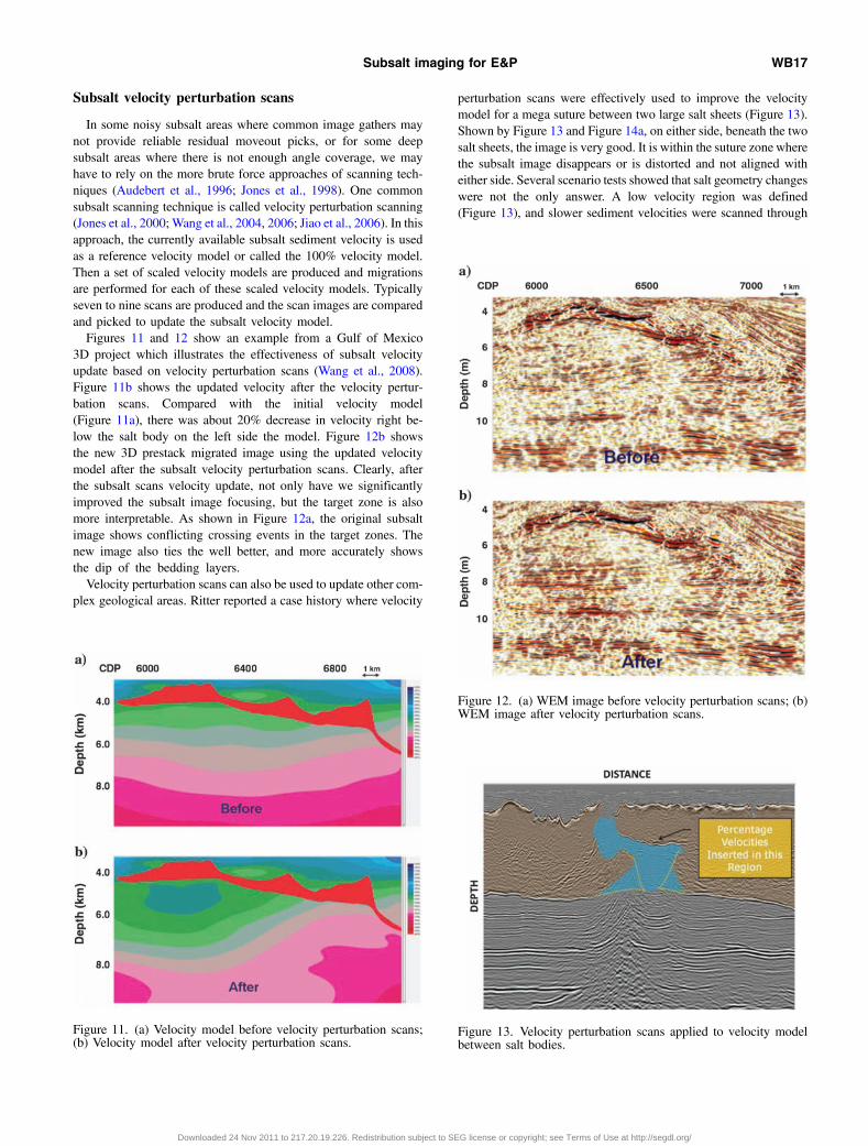
Subsalt velocity perturbation scans

In some noisy subsalt areas where common image gathers maynot provide reliable residual moveout picks, or for some deepsubsalt areas where there is not enough angle coverage, we mayhave to rely on the more brute force approaches of scanning tech-niques (Audebert et al., 1996; Jones et al., 1998). One commonsubsalt scanning technique is called velocity perturbation scanning(Jones et al., 2000; Wang et al., 2004, 2006; Jiao et al., 2006). In thisapproach, the currently available subsalt sediment velocity is usedas a reference velocity model or called the 100% velocity model.Then a set of scaled velocity models are produced and migrationsare performed for each of these scaled velocity models. Typicallyseven to nine scans are produced and the scan images are comparedand picked to update the subsalt velocity model.Figures 11 and 12 show an example from a Gulf of Mexico

3D project which illustrates the effectiveness of subsalt velocityupdate based on velocity perturbation scans (Wang et al., 2008).Figure 11b shows the updated velocity after the velocity pertur-bation scans. Compared with the initial velocity model(Figure 11a), there was about 20% decrease in velocity right be-low the salt body on the left side the model. Figure 12b showsthe new 3D prestack migrated image using the updated velocitymodel after the subsalt velocity perturbation scans. Clearly, afterthe subsalt scans velocity update, not only have we significantlyimproved the subsalt image focusing, but the target zone is alsomore interpretable. As shown in Figure 12a, the original subsaltimage shows conflicting crossing events in the target zones. Thenew image also ties the well better, and more accurately showsthe dip of the bedding layers.Velocity perturbation scans can also be used to update other com-

plex geological areas. Ritter reported a case history where velocity

perturbation scans were effectively used to improve the velocitymodel for a mega suture between two large salt sheets (Figure 13).Shown by Figure 13 and Figure 14a, on either side, beneath the twosalt sheets, the image is very good. It is within the suture zone wherethe subsalt image disappears or is distorted and not aligned witheither side. Several scenario tests showed that salt geometry changeswere not the only answer. A low velocity region was defined(Figure 13), and slower sediment velocities were scanned through

Figure 11. (a) Velocity model before velocity perturbation scans;(b) Velocity model after velocity perturbation scans.

Figure 12. (a) WEM image before velocity perturbation scans; (b)WEM image after velocity perturbation scans.

Figure 13. Velocity perturbation scans applied to velocity modelbetween salt bodies.



this region. A percentage velocity was found that allowed the mar-ker events below the suture zone to be consistent with the surround-ing sediment. This allowed a more geologically reasonable saltinterpretation to be put in-place. Figure 14b is the migration imageafter the velocity perturbation scans, in which the subsalt continuityhas been greatly improved.

RTM-based delayed imaging time scans

Although the velocity perturbation scan technique is promising,the cost of generating a seismic migration scan is still comparativelyhigh, and it requires multiple prestack migration runs. To addressthe cost issues, Wang et al. (2006, 2009) have developed a new effi-cient subsalt velocity updating approach using RTM-based delayedimaging time (DIT) scans. In DIT scan, only one RTM run is per-formed, but multiple migration scan images are formed by applyingzero time as well as nonzero time (such as −200 ms or þ200 ms)(Sava and Fomel, 2006; Wang et al., 2006) imaging conditions, asexplained earlier. Since application of additional imaging condi-tions can be performed at a very small fraction of the cost as com-pared with the whole RTM run, typically dense scans (such as 21scans) are produced.Figure 15 shows an example of DIT-scan panels. Clearly, for this

example, with the negative time-shift, the subsalt events are muchbetter focused. Figure 16 shows a 3D example from Gulf of Mexico,comparing the RTM images before and after the DIT subsalt velo-city update. In the highlighted target area, after the DIT scans, theRTM image is much more interpretable, and our interpreters believethe new structure makes more geological sense.

CONCLUSIONS

In this paper we have presented the fundamental ideas underlyingsubsalt imaging. The physical problem caused by the presence ofthick allochtonous salt sheets surrounded by acoustic softer sedi-ments is an illumination issue related to the geometry of the sedi-ment-salt interface. We have summarized the four types of prestackdepth imaging algorithms that are currently the industry’s preferredimaging methods and described their strengths and weaknesses. Inaddition the rich spectrum of imaging conditions was investigated.Finally, we have described the elements of the model building and

Figure 15. An example of DIT-scan panels with delayed imagingtime: (a) 0 ms; (b)þ100 ms; (c)−100 ms.

Figure 16. (a) RTM image before DIT scans; (b) RTM image afterDIT scans.Figure 14. (a) RTM image before velocity perturbation scans; (b)

RTM image after velocity perturbation scans.



some techniques for subsalt velocity updates. While a huge amountof progress has been made in this field, yielding great improvementin image quality, we fully expect that the subsalt challenge will con-tinue to spur new theoretical developments and processing techni-ques, in the quest for yet more accurate and precise subsurfaceimages.

REFERENCES

Albertin, U., S. J. Kapoor, and W. Chang, 1998a, Velocity resolution and saltboundary placement in subsalt imaging: Part 1: 68th Annual InternationalMeeting, SEG, Expanded Abstracts, 1297–1300.

Albertin, U., S. J. Kapoor, W. Chang, R. Beals, and J. Curtis, 1998b,Velocity resolution and salt boundary placement in subsalt imaging:Part 2: 68th Annual International Meeting, SEG, Expanded Abstracts,1301–1304.

Albertin, U., M. Woodward, J. Kapoor, W. Chang, S. Charles, D. Nichols,P. Kitchenside, and W. Mao, 2001, Depth imaging examples andmethodology in the Gulf of Mexico: The Leading Edge, 20, 498–513,doi: 10.1190/1.1438980.

Anderson, J. E., and C. M. Marcinkovich, 2005, Finding the edge of salt viaa dual-velocity flood: 75th Annual International Meeting, SEG, ExpandedAbstracts, 1974–1977.

Audebert, F., and J. P. Diet, 1996, CRP-scan from 3D prestack depthmigration: A new tool for velocity model building: 58th Annual Interna-tional Conference, EAGE, Extended Abstracts, X011.

Baysal, E., D. Kosloff, and J. W. C. Sherwood, 1983, Reverse-timemigration: Geophysics, 48, 1514–1524, doi: 10.1190/1.1441434.

Beylkin, G., 1985, Imaging of discontinuities in the inverse scatteringproblem by inversion of a causal generalized radon transform: Journalof Mathematical Physics, 26, 99–108, doi: 10.1063/1.526755.

Billette, F. J., and S. Brandsberg-Dahl, 2005, The 2004 BP velocitybenchmark: 67th EAGE Meeting, B035.

Biondi, B., 2011, Velocity estimation by image focusing analysis:Geophysics, 75, no. 6, U49-U60.

Bleistein, N., 1987, On the imaging of reflectors in the earth: Geophysics,52, 931–942, doi: 10.1190/1.1442363.

Cerveny, V., M. M. Popov, and I. Psencik, 1982, Computation of wave fieldsin inhomogeneous media Gaussian beam approach: Geophysical Journalof the Royal Astronomical Society, 70, 109–128.

Claerbout, J. F., 1971, Toward a unified theory of reflector mapping:Geophysics, 36, 467–481, doi: 10.1190/1.1440185.

Claerbout, J. F., 1985, Imaging the earth’s interior: Blackwell ScientificPublications.

Cohen, J. K., F. G. Hagin, and N. Bleistein, 1986, Three dimensional borninversion with an arbitrary reference: Geophysics, 51, 1552–1558, doi:10.1190/1.1442205.

Corcoran, C., C. Perkins, D. Lee, P. Cattermole, R. Cook, and R. Moldo-veanu, 2007, Awide-azimuth streamer acquisition pilot project in the Gulfof Mexico: The Leading Edge, 26, 460–468, doi: 10.1190/1.2723210.

Costa, C. A., S. Raz, and D. Kosloff’, 1989. Gaussian beam migration: 59thAnnual International Meeting, SEG, Expanded Abstracts, 1169–1171.

de Bruin, C., C. Wapenaar, and A. J. Berkhout, 1990, Angle-dependentreflectivity by means of prestack migration: Geophysics, 55, 1223–1234, doi: 10.1190/1.1442938.

Fomel, S., 2004, Theory of 3-d angle gathers in wave-equation imaging:74th Annual International Meeting, SEG, Expanded Abstracts,1053–1056.

French, W. S., 1974, Two-dimensional and three-dimensional migration ofmodel-experiment reflection: Geophysics, 39, 265–277, doi: 10.1190/1.1440426.

Hale, D., N. R. Hill, and J. P. Stefani, 1992, Imaging salt with turningseismic waves: Geophysics, 57, 1453–1462, doi: 10.1190/1.1443213.

Haugen, J. A., B. Arntsen, and J. Mispel, 2008, Modeling of dirtysalt: 78th Annual International Meeting, SEG, Expanded Abstracts,2127–2131.

Hemon, C., 1978, Wave equations and models: Geophysical Prospecting,26, 790–821, doi: 10.1111/gpr.1978.26.issue-4.

Hill, N. R., 1990, Gaussian beam migration: Geophysics, 55, 1416–1428,doi: 10.1190/1.1442788.

Howard, M., and N. Moldoveanu, 2006, Marine survey design for rich-azimuth seismic using surface streamers: The Leading Edge, 25,2915–2919.

Hudec, M. R., and M. P. A. Jackson, 2007, Terra infirma: undderstandingsalt tectonics: Earth-Science Reviews, 82, 1–28, doi: 10.1016/j.earscirev.2007.01.001.

Jiao, J., D. Lowrey, J. Willis, and D. Solan, 2006, An improved methodologyfor sub-salt velocity analysis: 76th Annual International Meeting, SEG,Expanded Abstracts, 3105–3108.

Jones, I. F., 2008, A modeling study of pre-processing considerationsfor reverse-time migration: Geophysics, 73, no. 6 T99–T106, doi:10.1190/1.2981183.

Jones, I. F., 2010, An introduction to velocity model building: EuropeanAssociation of Geoscientists & Engineers.

Jones, I. F., H. Baud, K. Ibbotson, and F. Audebert, 2000, Conti-nuous 3D preSDM velocity analysis: The Leading Edge, 19, no. 3,263–269, doi: 10.1190/1.1438584.

Jones, I. F., K. Ibbotson, M. Grimshaw, and P. Plasterie, 1998, 3D pre-stackdepth migration and velocity model building: The Leading Edge, 17,897–911, doi: 10.1190/1.1438063.

Kapoor, J., N. Moldevaneau, M. Egan, M. O’Briain, D. Desta,L. Atakishiyev, M. Tomida, and L. Stewart, 2007, Subsaltimaging: The RAZ-WAZ experience: The Leading Edge, 26,1414–1422, doi: 10.1190/1.2805764.

Kapoor, J., and M. Woodward, 2008, Velocity model building for subsaltimaging using wide and rich azimuth data: 78th Annual InternationalMeeting, SEG, Expanded Abstracts, 3693–3696.

Kelly, S., and R. Jiaxiang, 2004, Key elements in the recovery of relativeamplitude for prestack shot record migration: The Leading Edge, 23,882–886, doi: 10.1190/1.1803497.

Leveille, J. P., K. Larner, and J. Higgingbotham, 2005, A problemworkshop:The Leading Edge, 24, 1126–1132, doi: 10.1190/1.2135107.

Lewis, J., 2006, The potential of mode-converted waves in salt interpreta-tion: Presented at SEG/EAGE summer research workshop.

Liu, F., G. Zhang, S. A. Morton, and J. P. Leveille, 2011, An effectiveimaging condition for reverse-time migration using wavefield decompo-sition: Geophysics, 76, no. 1, S29–S39, doi: 10.1190/1.3533914.

McMechan, G. A., 1983, Migration by extrapolation of time-dependentboundary values: Geophysical Prospecting, 31, 413–420, doi: 10.1111/gpr.1983.31.issue-3.

Moldoveanu, N., J. Kapoor, and M. Egan, 2008, Full-azimuthimaging using circular geometry acquisition: The Leading Edge, 27,908–913, doi: 10.1190/1.2954032.

Nolan, C., and W. Symes, 1996, Imaging in complex velocities withgeneral acquisition geometry: Trip, The Rice Inversion Project, RiceUniversity.

Pratt, R. G., 2003, Waveform tomography: Theory and practice. An invitedpresentation given at the 12th international workshop on controlled-source seismology: Mountain Lake, Virginia (web link @ http://geol.queensu.ca/people/pratt/prattccss.pdf).

Rickett, J. E., and P. C. Sava, 2002, Offset and angle-domaincommon image-point gathers for shot-profile migration: Geophysics,67, 883–889, doi: 10.1190/1.1484531.

Ritter, G., 2010, Interpretation driven velocity model building to improvesubsalt imaging: 81st Annual International Meeting, SEG, ExpandedAbstracts, 4098–4102.

Sava, P., and S. Fomel, 2003, Angle-domain common-image gathersby wave field continuation methods: Geophysics, 68, 1065–1074, doi:10.1190/1.1581078.

Sava, P., and S. Fomel, 2006, Time-shift imaging condition in seismicmigration: Geophysics, 71, no. 6, S209–S217, doi: 10.1190/1.2338824.

Sava, P., and I. Vasconcelos, 2011, Extended imaging conditions for wave-equation migration: Geophysical Prospecting, 59, 35–55, doi: 10.1111/gpr.2010.59.issue-1.

Schneider, W. A., 1978, Integral formulation for migration in two and threedimensions: Geophysics, 43, 49–76, doi: 10.1190/1.1440828.

Sexton, P., B. Duquet, J. L. Bouroullec, F. Adler, V. Martin, and M. Stankoff,2009, Block 32, angola–a case study in complex imaging: EAGE, SubsaltImaging Workshop, SS29.

Sherwood, J. W. C., K. Sherwood, H. Tieman, and K. Schleicher, 2008, 3dbeam prestack depth migration with examples from around theworld: 78th Annual International Meeting, SEG, Expanded Abstracts,438–442.

Wang, B., V. Dirks, P. Guillaume, F. Audebert, and D. Epili, 2006, A 3Dsubsalt tomography based on wave-equation migration-perturbationscans: Geophysics, 71, no. 2, E1–E6, doi: 10.1190/1.2187720.

Wang, B., V. Dirks, P. Guillaume, F. Audebert, A. Hou, and D. Epili, 2004,3D sub-salt tomography based on wave equation migration perturbationscans: 74th Annual International Meeting, SEG, Expanded Abstracts,2375–2378.

Wang, B., Y. Kim, C. Mason, and X. Zeng, 2008, Advances in velocitymodel-building technology for subsalt imaging: Geophysics, 73, no. 5,VE173–VE181, doi: 10.1190/1.2966096.

Wang, B., C. Mason, M. Guo, K. Yoon, J. Cai, J. Ji, and Z. Li, 2009, Subsaltvelocity update and composite imaging using reverse-time-migration based delayed-imaging-time scan: Geophysics, 74, no. 6,WCA159–WCA167, doi: 10.1190/1.3227152.

Wang, B., D. Wheaton, F. Audebert, and V. Dirks, 2006, Separation offocusing and positioning effects using wave equation based focusinganalysis and post-stack modeling: 76th Annual International Meeting,SEG, Expanded Abstracts, 2646–2649.



http://dx.doi.org/10.1190/1.1438980

http://dx.doi.org/10.1190/1.1438980

http://dx.doi.org/10.1190/1.1438980

http://dx.doi.org/10.1190/1.1441434

http://dx.doi.org/10.1190/1.1441434

http://dx.doi.org/10.1190/1.1441434

http://dx.doi.org/10.1063/1.526755

http://dx.doi.org/10.1063/1.526755

http://dx.doi.org/10.1063/1.526755

http://dx.doi.org/10.1190/1.1442363

http://dx.doi.org/10.1190/1.1442363

http://dx.doi.org/10.1190/1.1442363

http://dx.doi.org/10.1190/1.1440185

http://dx.doi.org/10.1190/1.1440185

http://dx.doi.org/10.1190/1.1440185

http://dx.doi.org/10.1190/1.1442205

http://dx.doi.org/10.1190/1.1442205

http://dx.doi.org/10.1190/1.1442205

http://dx.doi.org/10.1190/1.2723210

http://dx.doi.org/10.1190/1.2723210

http://dx.doi.org/10.1190/1.2723210

http://dx.doi.org/10.1190/1.1442938

http://dx.doi.org/10.1190/1.1442938

http://dx.doi.org/10.1190/1.1442938

http://dx.doi.org/10.1190/1.1440426

http://dx.doi.org/10.1190/1.1440426

http://dx.doi.org/10.1190/1.1440426

http://dx.doi.org/10.1190/1.1440426

http://dx.doi.org/10.1190/1.1443213

http://dx.doi.org/10.1190/1.1443213

http://dx.doi.org/10.1190/1.1443213

http://dx.doi.org/10.1111/gpr.1978.26.issue-4





http://dx.doi.org/10.1190/1.1442788

http://dx.doi.org/10.1190/1.1442788

http://dx.doi.org/10.1190/1.1442788

http://dx.doi.org/10.1016/j.earscirev.2007.01.001






http://dx.doi.org/10.1190/1.2981183

http://dx.doi.org/10.1190/1.2981183

http://dx.doi.org/10.1190/1.2981183

http://dx.doi.org/10.1190/1.1438584

http://dx.doi.org/10.1190/1.1438584

http://dx.doi.org/10.1190/1.1438584

http://dx.doi.org/10.1190/1.1438063

http://dx.doi.org/10.1190/1.1438063

http://dx.doi.org/10.1190/1.1438063

http://dx.doi.org/10.1190/1.2805764

http://dx.doi.org/10.1190/1.2805764

http://dx.doi.org/10.1190/1.2805764

http://dx.doi.org/10.1190/1.1803497

http://dx.doi.org/10.1190/1.1803497

http://dx.doi.org/10.1190/1.1803497

http://dx.doi.org/10.1190/1.2135107

http://dx.doi.org/10.1190/1.2135107

http://dx.doi.org/10.1190/1.2135107

http://dx.doi.org/10.1190/1.3533914

http://dx.doi.org/10.1190/1.3533914

http://dx.doi.org/10.1190/1.3533914







http://dx.doi.org/10.1190/1.2954032

http://dx.doi.org/10.1190/1.2954032

http://dx.doi.org/10.1190/1.2954032

http://geol.queensu.ca/people/pratt/prattccss.pdf




http://dx.doi.org/10.1190/1.1484531

http://dx.doi.org/10.1190/1.1484531

http://dx.doi.org/10.1190/1.1484531

http://dx.doi.org/10.1190/1.1581078

http://dx.doi.org/10.1190/1.1581078

http://dx.doi.org/10.1190/1.1581078

http://dx.doi.org/10.1190/1.2338824

http://dx.doi.org/10.1190/1.2338824

http://dx.doi.org/10.1190/1.2338824







http://dx.doi.org/10.1190/1.1440828

http://dx.doi.org/10.1190/1.1440828

http://dx.doi.org/10.1190/1.1440828

http://dx.doi.org/10.1190/1.2187720

http://dx.doi.org/10.1190/1.2187720

http://dx.doi.org/10.1190/1.2187720

http://dx.doi.org/10.1190/1.2966096

http://dx.doi.org/10.1190/1.2966096

http://dx.doi.org/10.1190/1.2966096

http://dx.doi.org/10.1190/1.3227152

http://dx.doi.org/10.1190/1.3227152

http://dx.doi.org/10.1190/1.3227152

Whitmore, D., 1983, Iterative depth migration by backward time propaga-tion: 53rd Annual International Meeting, SEG, Expanded Abstracts,382–385.

Woodward, M., D. Nichols, O. Zdraveva, P. Whitfield, and T. Johns, 2008, Adecade of tomography: Geophysics, 73, no. 5, VE5–VE11, doi: 10.1190/1.2969907.

Xu, S., H. Chauris, G. Lambare, and M. Noble, 2001, Common-anglemigration: A strategy for imaging complex media: Geophysics, 66,1877–1894, doi: 10.1190/1.1487131.

Xu, S., Y. Zhang, and B. Tang, 2010, 3D common image gathers from re-verse time migration: 81st Annual International Meeting, SEG, ExpandedAbstracts, 3257–3262.

Zhang, Q., and G. A. McMechan, 2011, A DCIG for isotropic RTM directvectorfield method to obtain angle-domain common-image gathers

from isotropic acoustic and elastic reverse-time migration: Geophysics,submitted.

Zhang, Y., and J. Sun, 2009, Practical issues of reverse-time migration: Trueamplitude gathers, noise removal and harmonic-source encoding: FirstBreak, 26, 19–25.

Zhang, Y., S. Xu, N. Bleistein, and G. Zhang, 2007, True-amplitude,angle-domain, common-image gathers from one-way wave-equationmigrations: Geophysics, 72, no. 1, S49–S58, doi: 10.1190/1.2399371.

Zhang, Y., G. Zhang, and N. Bleistein, 2002, Theory of true amplitudecommon-shot migration: 72nd Annual International Meeting, SEG,Expanded Abstracts, 2471–2474.

Zhang, Y., G. Zhang, and N. Bleistein, 2005, Theory of true amplitudeone-way wave equations and true amplitude common-shot migration:Geophysics, 70, no. 4, E1–E10, doi: 10.1190/1.1988182.



http://dx.doi.org/10.1190/1.2969907

http://dx.doi.org/10.1190/1.2969907

http://dx.doi.org/10.1190/1.2969907

http://dx.doi.org/10.1190/1.2969907

http://dx.doi.org/10.1190/1.1487131

http://dx.doi.org/10.1190/1.1487131

http://dx.doi.org/10.1190/1.1487131

http://dx.doi.org/10.1190/1.2399371

http://dx.doi.org/10.1190/1.2399371

http://dx.doi.org/10.1190/1.2399371

http://dx.doi.org/10.1190/1.1988182

http://dx.doi.org/10.1190/1.1988182

http://dx.doi.org/10.1190/1.1988182

Subsalt imaging for exploration, production, and ... Center/Technical... · Subsalt imaging for...

Documents

Transcript of Subsalt imaging for exploration, production, and ... Center/Technical... · Subsalt imaging for...