1

Subsalt Seismic Illumination Study

Ana Belen Sanz Fernandez

ABSTRACT

Subsalt seismic illumination is a challenge when the salt structure becomescomplicated. Even using the most advanced seismic acquisition and imaging technologyit is difficult to visualize subsalt targets. An illumination study can reduce explorationrisk by identifying shadow areas and testing scenarios that lead to optimum imagequality.

Illumination analysis can also help to accurately interpret the seismic image,Advanced imaging algorithms like reverse time migration can introduce noise at steepdip, high contrast impedance boundaries such as the salt-sediment interface. Theseartifacts can be confused with valid structural features.

This study will test the hypothesis that a combination 3D ray tracing and finitedifference modeling can identify poorly illuminated subsalt areas. My work will not onlyinvestigate the nature and origin of shadow zones, but also try to improve signal recoveryin those regions.

Background

The interface between the sediment layers and the complex salt structure, distortsthe seismic ray path, due to the high acoustic impedance contrast. For that reason,associated with the salt-edge, there are some issues that should be considered in a subsaltillumination study (Muerdter & Ratcliff, 2001; and Muerdter et al., 2001):

- Maximum angle of illumination decreases.- Fold reduction, due to the low signal-to-noise ratio.- Greatly reduced amplitude (transmission losses through sediment-salt

interface). The equalization algorithms in seismic processing usually enhanceboth the weaker signal and the noise.

- Salt structure effect reaches the rays located less than one half of themaximum offset away from the edge of the structure.

- Shape of the base of the salt distorts more the signal comparing with the top.A combination of both dipping in different directions can produce seriousdisruptions.

- Poor illuminated areas increases when the dipping angle of the edge is closerto the critical angle.

Sigsbee2A model, released by SMAART JV Consortium in 2001, is an constantdensity acoustic dataset, that does not contain free surface multiples and almost nointernal multiples due to very low contrast water bottom, that illustrates the illumination

2

issues associated with salt structures (Figure 1). This model includes a rugous salt, whichbase presents flat and steep dip areas. It also presents difractors, faults and subsaltstructures.

Figure 1. Sigsbee 2A Model (released by SMAART JV Consortium, 2001).

A ray tracing study is a cheap technique that simulates the ray path from thesubsalt reflector to the surface (Gjøystdal et al., 2002). This methodology helps toevaluate the risk, and can be performed after acquisition to identify the issues that affectsthe interpretation. According to Jin & Walraven (2003), the results of ray tracing definethe shadow zones. In Figure 2, the results of the total illumination map from all incidenceangles show the subsalt poor illuminated areas.

Figure 2. Synthetic subsalt Illumination Example (Jin & Walraven, 2003).The shadow zones are highlighted.

3

The geometrical reasons, that explain those subsalt shadow areas, are driven bythe critical angle calculation (c) computed from Snell’s law. The critical angle is definedas:

Where vlayer and vsalt are the instantaneous velocities at certain point located in theinterface between the sediment and the salt body.

The maximum dip-angle (max) that can be illuminated under the salt structurewould be defined by the following expression:

max = c – sed

Where sed represents the dip-angle of the subsalt reflectors.

Ray tracing only can simulate the ray path in one way. Full wave equationcompleted the study with multiarrivals computation. The results of finite differencemodeling (Figure 3), show good image of the top, good amplitude at the base of salt, andgood collapse of diffractors. The shadow areas (surrounded by black ellipses), coincidewith the ray tracing results. Also, the amplitude reciprocity is not correct in areas locatedunder high dipping structure (shadow areas) with high acoustic impedance interfaces(Muerdter et al., 2001).

Figure 3. Finite Difference Modeling. (Jin & Walraven, 2003)

The advantage of wave-equation migration is the ability to handle amplitudes,multivalued arrivals, and anti-aliasing issues in one pass (Pharez et al., 2005). Besideswave equation, there are other migration algorithms, well-known in the industry likeKirchhoff depth migration.This algorithm computes a subset volume (affording time). Onthe other hand, Kirchhoff only integrates energy that has travel along one path.

4

Reverse time migration (Baysal et al., 1983; Whitmore, 1983) is the mostadvanced migration algorithm. It is based on shot gather migration technique (Jacobs,1982; Etgen, 1986), where each profile is migrated individually and then sum the imagedcubes obtained for all shots (Biondi, 2007). It can handle both multiarrivals and prismaticwaves. Also, it can illuminate steep dipping structures. On the other hand, reverse timemigration is an expensive algorithm.

Also, reverse time migration can present artificial reflections coming from theboundaries of the domain (Clapp and Fu, 2010). There are different techniques trying toresolve this problem: introducing a damping region around the computation domain(Cerjan et al., 1985); introducing a boundary condition that attempts to kill energypropagating at some limited range of angles perpendicular to the boundary (Clayton andEngquist, 1980); or most effectively, and expensive, applying perfectly matched limit(PML) (Berenger, 1996), which simulates propagating a complex wave whose energydecreases as it approaches to the boundary.

Yan & Xie (2009) affirmed that reverse time migration produces lowwavenumber artifacts that mask the geological structure. This issue became critical inhigh velocity contrasts or in high gradient, like in salt structures.

Anisotropy is one of the most important factor that impacts in velocity mapping,and in some cases, it also affects on the focusing velocity (Biondi, 2007). Verticaltransverse isotropic improves the quality of the image considering the velocity travel timedifferences between the vertical and horizontal directions. This assumption does notinclude the velocity delay produced in the steep dip layered strata (TTI or tilted polaraxis).

Case Study

The area of interest is located in the Mississippi Canyon (Gulf of Mexico). Itpresents alochtonous salt bodies. The sediments have been deposited since Late Jurassic.The strata are composed by a siliciclastic interbedding of sands and shales, deposited in aturbidite system. The salt displacements generated some extensive normal faults, crossingthe sediment layers.

The available dataset are two stack depth volumes, located in the sameexploration area in Gulf of Mexico. Both volumes correspond to the same acquisitionsurvey (narrow azimuth), applying the same time processing and generating the sameshot gathers. They have been migrated applying the same vp velocity field (Figure 4),which is anisotropic (vertical transverse isotropic). The difference between them is thealgorithm used in the migration: Pre-stack anisotropic kirchhoff depth migration (Figure5) and Anisotropic reverse time migration (Figure 6). The seismic processing sequenceappears at the end of this proposal (see attachment).

5

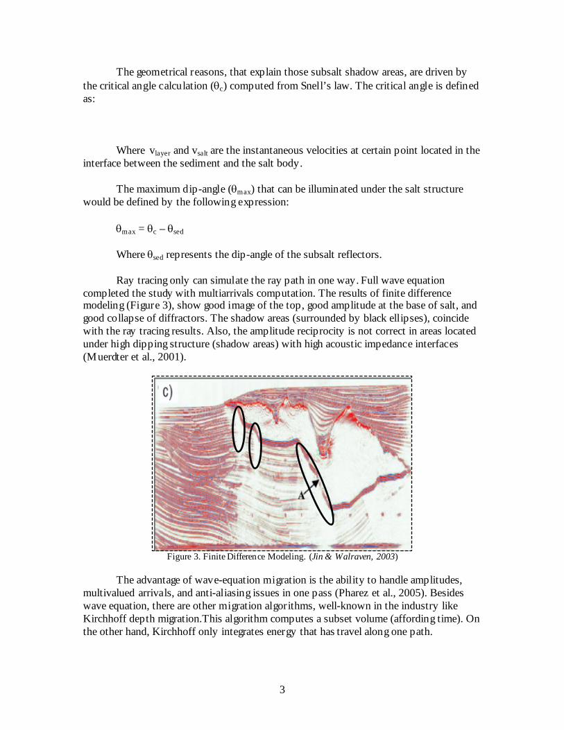
It is important to highlight that the studied area covers a small part of the totalsurvey and does not have any well data in the proximities. Also, there is no seismicgather available for this study.

Figure 4. 2D slice of the 3D anisotropic vp velocity field.

The figures 5 and 6 show the seismic volumes anisotropy Kirchhoff depthmigration and anisotropy reverse time migration (respectively). The top of the salt bodiesare well defined in both images. Also, the bases of salt bodies present a good image.Anisotropy Kirchhoff depth migration has higher frequency and presents a betterdefinition of the sediments in the areas that are not influenced by the salt bodies. As itwas expected, anisotropy reverse time migration improves the continuity of the subsaltsediment layers.

6

Figure 5. 3D Anisotropic Kirchhoff Pre-Stack Depth Migration. 2D slice is shown coincident with velocitymodel in Figure 4.

Figure 6. 3D Anisotropic reverse Time Migration shown along same line as Figure 5.Areas of illumination study highlighted

Besides the differences, both algorithms present some shallower stratificationwith an increasing sediment wedge associated to the structure (Figures 5 and 6 upper

7

right). The terminations of the layers are folded and change in depth. On the other hand,Kirchhoff can not illuminate the sedimentological terminations against the salt, showing anoisy image. Reverse time migration shows steep dip planes, opposite to thestratification, presenting a parallel angle that does not fit to the layer terminations. Theangle of those planes is different than the fault planes.

Objectives

So, the main objective consists on: to demonstrate with a complete illuminationstudy that the steep dip planes, present in anisotropy reverse time migration, areartifacts (they are not representing any geological structure).

A secondary objective is the subsalt shadow areas definition, specifying themaximum dipping angle that can be illuminated.

After resolving that question, a third objective is subsalt image quality improve inthe shadow areas.

Methodology

As in the Seigsbee2A Model (Smaart JV Consortium, 2001), a completeillumination study will help to understand the subsalt imaging problems. Also, Muerdteret al. (2001) develop a successful illumination study using ray tracing modeling.

The first step of the workflow is to find the maximum subsalt dip angle. A 3D raytracing study will be performed to calculate that limit (see areas of illumination study inFigure 6).

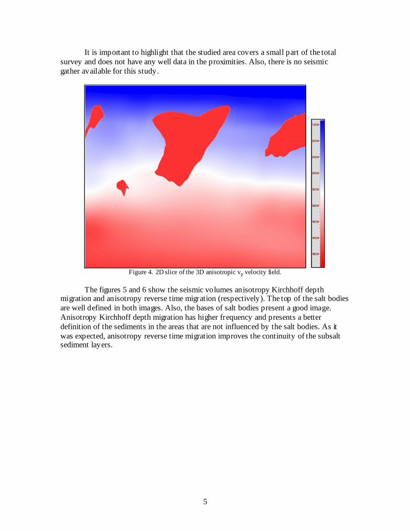
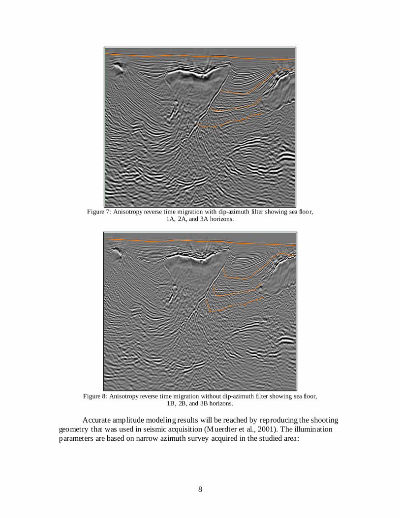
For this porpoise, a set of three horizons will be picked different flat levels(increasing in depth: 1A, 2A, 3A) present in the anisotropy reverse time migration stackvolume. Anisotropy reverse time migration has been enhanced applying a structural filter,which respects the structure (observe that the faults are still present in the Figure 7) andimproves the continuity of the stratification, eliminating partially the high dipping planes.The continuous line represents the sea floor, and the dash lines show the proposedhorizons that will be picked for the study. Also, another equivalent set of three horizons(1B, 2B, 3B) will be picked but following the steep dip planes. Basically, the differencesbetween A and B will be the termination against the salt body (see Figure 8).

8

Figure 7: Anisotropy reverse time migration with dip-azimuth filter showing sea floor,1A, 2A, and 3A horizons.

Figure 8: Anisotropy reverse time migration without dip-azimuth filter showing sea floor,1B, 2B, and 3B horizons.

Accurate amplitude modeling results will be reached by reproducing the shootinggeometry that was used in seismic acquisition (Muerdter et al., 2001). The illuminationparameters are based on narrow azimuth survey acquired in the studied area:

9

- Shooting angle:Dip range: 0 – 30o (step: 1o)Azimuth range: -45o – 135o (step: 5o)

The vertical transverse isotropic velocity field will be included as a second part ofthe model. The interval velocity volumes (epsilon and delta) will be incorporated in thecomputation to study the anisotropy effect at the different levels in both 3D ray tracinganalysis (high and low dip events).

Expected results and early recommendations

As expected results, 3D ray tracing will obtain a high fold value in the steepplanes. The ray path, from plane-termination to surface, will be registered inside theaperture diameter. On the other hand, a ray path from a source located at the flattermination of the sediment layers, will travel to the salt body and then, probably wouldeither way: bounced back (and then will reach the surface out of the aperture) or travelthrough the salt body; in both cases, it will be difficult to recover the signal.

The flat events will be difficult to illuminate, while the steep planes will beclearly illuminated. But the quality of the seismic image is poor in the shadow zone (lowfold). So, ray tracing results could demonstrate that the steep planes are artifacts.

The improvement of the illumination recovering could be resolved simulating thefollowing wide azimuth acquisition parameters:

IL100m

8000m

IL100m

8000m

10

Those parameters are similar to another seismic acquisition survey developed inthe studied area.

Also, the wide azimuth illumination study would include the vertical transverseisotropic velocity field, as a second part of the analysis. A priori, p-wave velocity in wideazimuth presents more variations depending on the direction of propagation.

The analysis of the results of the wide azimuth illumination would help to proposea possible solution to recover a better signal at the surface and therefore, improve thesubsalt illumination.

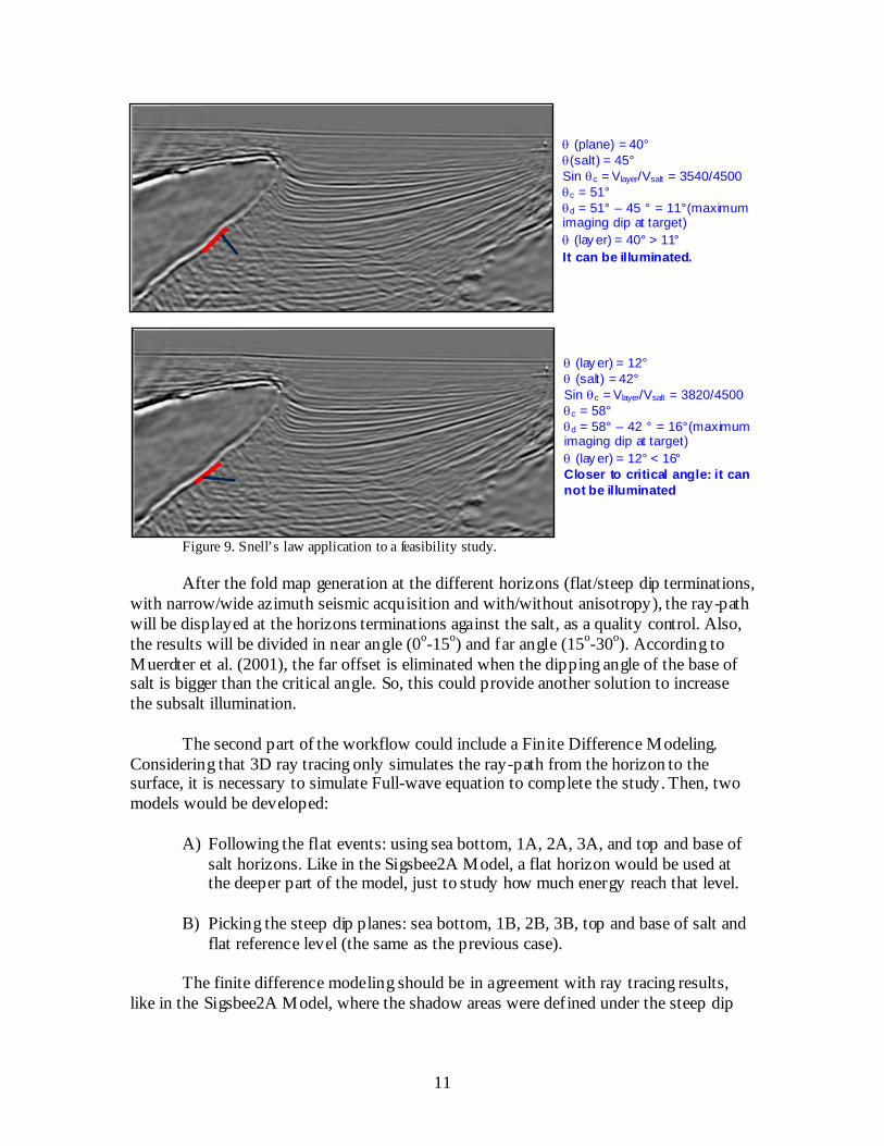
Finally, it is possible to calculate the limit angle, considering the inclination of thebase of salt, the dip of the sediment against the salt, and the interval velocities of thesediment and the salt (Snell’s law). Figure 9 shows the results of a subsalt study for twodifferent angle terminations. The steep dip plane can be illuminated: the dip-angle plane(plane = 40°) is greater than the critical angle (c = 51°). On the other hand, the low diptermination (layer = 12°) has angle smaller than the critical angle (c = 58°), so the flatevents can not be illuminated (defining a shadow area).

IL100m

8000m

CL450

m

4200

m IL100m

8000m

IL100m

8000m

CL450

m

4200

m

11

Figure 9. Snell’s law application to a feasibility study.

After the fold map generation at the different horizons (flat/steep dip terminations,with narrow/wide azimuth seismic acquisition and with/without anisotropy), the ray-pathwill be displayed at the horizons terminations against the salt, as a quality control. Also,the results will be divided in near angle (0o-15o) and far angle (15o-30o). According toMuerdter et al. (2001), the far offset is eliminated when the dipping angle of the base ofsalt is bigger than the critical angle. So, this could provide another solution to increasethe subsalt illumination.

The second part of the workflow could include a Finite Difference Modeling.Considering that 3D ray tracing only simulates the ray-path from the horizon to thesurface, it is necessary to simulate Full-wave equation to complete the study. Then, twomodels would be developed:

A) Following the flat events: using sea bottom, 1A, 2A, 3A, and top and base ofsalt horizons. Like in the Sigsbee2A Model, a flat horizon would be used atthe deeper part of the model, just to study how much energy reach that level.

B) Picking the steep dip planes: sea bottom, 1B, 2B, 3B, top and base of salt andflat reference level (the same as the previous case).

The finite difference modeling should be in agreement with ray tracing results,like in the Sigsbee2A Model, where the shadow areas were defined under the steep dip

(lay er) = 12° (salt) = 42°Sin c = Vlayer/Vsalt = 3820/4500c = 58°d = 58° – 42 ° = 16°(maximumimaging dip at target)

(lay er) = 12° < 16°Closer to critical angle: it cannot be illuminated

(plane) = 40°(salt) = 45°Sin c = Vlayer/Vsalt = 3540/4500c = 51°d = 51° – 45 ° = 11°(maximumimaging dip at target)

(lay er) = 40° > 11°

It can be illuminated.

12

base of salt. Also, the amplitude of the reference horizon would indicate the quality of theillumination.

Time-line

Proposal…………………………………………..…………………………Feb 17

Illumination study…………………………………………………………….1. Project generation………………………………………….………………..DONE2. Seismic data loading………………………………………………………...DONE3. Horizon data loading………………………………………..........................0.5 day4. Picking 4 horizons in 3D following flat events in ARTM (sea floor, 1B, 2B,

3B)………………………………………...………………………………...3weeks5. Pick the 3 equivalent horizons but following the high dip events present in

ARTM: 1A, 2A, 3A (the only difference is the termination against thesalt)……………………………………..…………………………………..2 weeks

6. Build the Model map (for 6 horizons)…………………………………….2 days7. Run full narrow azimuth geometry without anisotropy for 6 horizons (one at the

time)…………………………………………….……………………….1 day8. Run full narrow azimuth geometry with anisotropy for 6 horizons (one at the

time)……………………………………………………………………..2 days9. Run full wide azimuth geometry without anisotropy for 6 horizons (one at the

time)……………………………………………………………………..1 day10. Run full wide azimuth geometry with anisotropy for 6 horizons (one at the

time)……………………………………………………………………...2 days11. Run filter narrow azimuth geometry without anisotropy for 6 horizons (one at the

time)……………………………………………………………………….1 day12. Run filter narrow azimuth geometry with anisotropy for 6 horizons (one at the

time)……………………………………………………………………….2 days13. Run filter wide azimuth geometry without anisotropy for 6 horizons (one at the

time)……………………………………………………………………….1 day14. Run filter wide azimuth geometry with anisotropy for 6 horizons (one at the

time)………………………………………………………………………..2 days15. Take some images…………………………………………………..…….2-3 days16. Analysis and comparison results…………………………………….……...3 days17. Calculate Maximum dip illumination (Snell’s Law) for each horizon……1-2days

Finite difference modelling:18. 2D Model building………………………………………………….………?????19. Run the model A……………………………………………………………?????20. Run the model B……………………………………………………………?????21. Comparison results……………………………………………………….7 days

Thesis Writing…………………………………………………………….18 weeks22. Introduction.…………………………………………………………2weeks23. Methodology………………………………………………………..2weeks

13

24. Results……………………………………………………………….2weeks25. Thesis arguments……………………………………………………4 weeks26. Antithesis arguments (just references)………………………………4 weeks27. Compare with references results……………………………………2 weeks28. Conclusions…………………………………………………………..2weeks

Conclusions

Steep dip base of salt can cause a misinterpretation of subsalt target, due to thepoor illumination (shadow zones). In our case study, the sediment terminations againstthe salt body present two different dip angle trends (flat and steep) in the anisotropyreverse time migration image. Even using the best available algorithm, there are someillumination limitations difficult to resolve, due to both: the acoustic impedance contrastof the material and the signal incidence angle.

A complete illumination study has been proposed to demonstrate that the subsaltsteep dip events are the product of the computation noise. Also, this methodology canresolve another two objectives: to determine the subsalt illumination limitation and topropose techniques that improves the recovery signal.

ACKNOWLEDGEMENTS

I would like to thank Repsol for the support to develop this study, and TGS technologiesfor the permission to show the data.

REFERENCES

Baysal, E., Kosloff, D. D., and Sherwood, J., 1983, Reverse Time Migration, Geophysics,48, 1514-1524.Berenguer, J., P., 1996, Perfectly matched layer for the FDTD solution of wave-structureinteraction problems. IEEE Transactions on Antenas and Propagation, 44, 110 – 117.Biondi, B., 2004, 3D seismic imaging, Stanford Exploration Project, 356pp.Cerjan, C., D. Kosloff, R. Kosloff and M. Reshef, 1985, A non-reflecting boundaryconditions for discrete acoustic and elastic wave equations. Geophysics, 50, 705 – 708.Clapp, R. G. and H. Fu, 2010, Selecting the right hardware for reverse time migration,The Leading Edge.Clayton, R. and B. Engquist, 1980, Absorbing boundary conditions for wave equationmigration. Geophysics, 45, 895 – 904.Etgen, j., 1986, Pre-stack reverse time migration of shot profiles: Standford ExplorationProject, Report 50, 151-170, http://sep.stantford.edu/research/reports.Gjøystdal, H., Iversen, E., Laurain,R., Lecomte, I., Vinje V., and Åstebøl K., 2002,Review of ray theory applications in modeling and imaging of seismic data, StudiaGeophysica et Geodaetica, 46, 2, 113 – 164.Jacobs, B., 1982, The Pre-stack migration of profiles: Ph.D. thesis, Stantford University.Jin, S., and Walraven, D., 2003, Wave equation GSP prestack depth migration andillumination, The Leading Edge, 22, 604-610.

14

Pharez, S., N. Jones, V. Dirks, S. Zimine, H. Prigent, K. Ibbotson and J-P. Gruffeille,2005, Pre-stack wave-equation migration as a routine production tool, The Leading Edge24; no. 6; p. 608-613.

Ratcliff, D. W., Weber, D. J., and Sellers, K. D., 1995, Subsalt imaging via the world'slargest 3-D pre-stack depth migration project, SEG Expanded Abstracts 14, 1156.

Whitmore, N. D., 1983, Iterative depth migration by backward time propagation: 53rd

Annual International Meeting, Society of Exploration Geophysicists, ExpandedAbstracts, 382-385.Yan, R., and X. Xie, 2009, A new angle domain imaging condition for pre-stack reverse-time migration: 79 th Annual International Meeting, Society of Exploration Geophysicists,Expanded Abstracts.

ATTACHMENT

The seismic processing sequence has been divided in two main workflows:

A) Pre-stack Time Processing Sequence was performed by TGS:- Debubble- Noise attenuation- Surface related multiple elimination (SRME)- Noise attenuation- Velocity analysis- Radon de-multiple- Application of cold water statics- 3D bin sort – 12.5m CDP interval, 58/64 fold- Deterministic decon- Spherical divergence and gain correction- Grid data – 25m x 40m – diagonal grid- Input migration velocities- Kirchhoff pre-stack curved ray migration – 25m x 40m- Velocity analysis- Automatic velocity picking update at every CDP location- Output 3D velocity trace volume (SEGY: 12.5m by 20m by 4msec)- Output ETA velocity correction trace volume (SEGY: 12.5m by 20m by 4msec)- Radon de-multiple- Output migrated gathers with NMO/Radon- Mute and stack

B) Wave Equation Migration was processed by TGS:- Initial sediment velocity model: Kirchhoff 3D PSTM velocities with salt influenceremoved.

Wave Equation PSDM model building:- Iteration I –finite difference migration (FDMIG) for sediment model update (PSDM)- Start point for PSDM: Output 3D volume, gathers over entire area, 50m x 40m grid at20Hz. Velocity update on 1 km x 1km grid

15

- Iteration II–FDMIG for sediment model update (PSDM): Velocity update on 1km x1km grid.- Interpret salt top/model build: Top salt interpretation using FDMIG depth volume.

Salt Flood for Base Salt:- Iteration III- FDMIG (flood) for salt base interpretation: PSDM based salt flood model,100% shots input. Output 3D volume, gathers over entire area, 50m x 40m grid at 20 Hz- Interpret salt base/model build: Base salt interpretation using FDMIG “flood” depthvolume. Final model construction.- Iteration IV – FDMIG output final gathers for entire image area. Output angle gatherson a 50m x 40m grid @ 30 Hz. Angle stack analysis and volume generation. Output rawmigration.

C) Kirchhoff Depth Migration was computed by TGS:

KIRCHHOFF DEPTH MIGRATION- Input Gathers (from time processing sequence)- Input WEM sediment velocity field- Half of shots and half of receivers used for velocity/model building iterations

Build Anisotropic Velocity Model- Build 3D vertical model from well information- Migrate the data- Estimate anisotropic parameters delta and epsilon- Migrate select lines to verify results – iterate above if necessary

ITERATIONS I & II - Tomography UpdatesKIRCHHOFF VTI PSDM- Input 25m x 40m, 29 to 32 fold, 12 seconds- Output 50m x 40m, 29 to 32 fold, 16000m depth, 10m step- Migration aperture 8000m- 2 passes of Tomography to define sediment vertical velocity field- Update delta and epsilon if needed- Tomography inversions at 200m x 200m x 50m

ITERATION III - Define Top of SaltKIRCHHOFF VTI PSDM- Input 25m x 40m, 29 to 32 fold, 12 seconds- Output 50m x 40m, 29 to 32 fold, 16000m depth, 10m step- Migration aperture 10000m with turning wave- Interpret Top of salt.

ITERATION IV - Define Base of Salt (Salt Flood)KIRCHHOFF VTI PSDM- Input 25m x 40m, 29 to 32 fold, 12 seconds- Output 50m x 40m, 29 to 32 fold, 16000m depth, 10m step

16

- Migration aperture 8000m- Interpret Base of salt

ITERATION V – Define Top of Salt for OverhangsKIRCHHOFF VTI PSDM- Input 25m x 40m, 29 to 32 fold, 12 seconds- Output 50m x 40m, 29 to 32 fold, 16000m depth, 10m step- Migration aperture 8000m, with turning wave- Interpret Top of salt for overhangs

ITERATION VI – Modify Base of Salt in Overhang AreasKIRCHHOFF VTI PSDM- Input 25m x 40m, 29 to 32 fold, 12 seconds- Output 50m x 40m, 29 to 32 fold, 16000m depth, 10m step- Migration aperture 8000m with turning wave- Interpret Base of salt for overhangs

ITERATION VII – Subsalt Tomography UpdateKIRCHHOFF VTI PSDM- Input 25m x 40m, 29 to 32 fold, 12 seconds- Output 50m x 40m, 29 to 32 fold, 16000m depth, 10m step- Migration aperture 8000m- 1 pass of Tomography to define sediment velocity field below the salt- Tomography inversions at 200m x 200m x 50m

FINAL KIRCHHOFF PRE-STACK DEPTH MIGRATION WITH OVERHANGS.KIRCHHOFF VTI PSDM- Input all shots and receivers from SRME/Radon data, 12.5m x 40m, 58 to 64 fold, 12seconds- Gathers output 50m x 40m, 29 to 32 fold, 16000m depth, 10m step (this output volumeis not available).- Migration aperture 10000m, maximum dip 90 degrees with turning wave, frequency: 3– 60 Hz (central frequency: 20 Hz).- Interpolate stack volume to a 25m by 20m grid- Post stack cosmetics application

D) VTI Anisotropy Reverse Time Migration was generated by Repsol:- Input all shots and receivers from SRME/Radon data, 12.5m x 40m, 58 to 64 fold, 12seconds.- Migration aperture 8000m, maximum dip 90 degrees, frequency 3 – 35 Hz (centralfrequency: 8Hz).

- Stack output volume, 10m step.