Submarine Hull Design

Volker Bertram

1. Hull design aspects................................................................................................................. 2 1.1. Overview of problems and approaches ........................................................................... 2 1.2. General guidelines for submarine hull design................................................................. 4

2. Hydrodynamic assessment ................................................................................................... 10

2.1. Introduction to CFD methods........................................................................................ 10 2.2. Introduction to model tests ............................................................................................ 13

2.2.1. Similarity laws........................................................................................................ 13 2.2.2. Resistance and propulsion tests.............................................................................. 14 2.2.3. Submarine model testing at HSVA (Hamburg Ship Model Basin) ....................... 15

2.3. Flow analysis on the sonar part ..................................................................................... 18 3. Hull-appendages interference............................................................................................... 19

3.1. Analysis methods for fins in uniform flow ................................................................... 19 3.2. Interaction of hull and foils ........................................................................................... 20 3.3. RANSE simulations for hull-appendage interaction..................................................... 21

4. Analysis methods for snorkels ............................................................................................. 23 References ................................................................................................................................ 26

2

1. Hull design aspects

Many papers have been presented on the subject of submarines, but there has been very little on the basic design process, Arentzen and Mandel (1961), Jackson (1992). Most concept design is done within the confines of confidential establishments and therefore not made public. We attempt here to compile sufficient information concerning the hull design predominantly from a hydrodynamic point of view.

1.1. Overview of problems and approaches

The prediction of ship hydrodynamic performance can be broken down into the general areas of

- resistance and propulsion - seakeeping - manoeuvring

Morgan and Lin (1998) give a good short introduction to the historical development of techniques to the state of the art in the late 1990s. Resistance and propulsion, including aspects of acoustical signa-tures, are particularly important for submarines. The basic approaches can be roughly classified into:

• Empirical/statistical approaches

Design engineers need simple and reasonably accurate estimates e.g. of the power require-ments. Common approaches combine a rather simple physical model and regression analysis to determine required coefficients either from one parent ship or from a set of ships. The co-efficients may be given in form of constants, formulae, or curves.

Because of the success with model testing, experimental series of surface ship hull forms were developed for varying hull parameters. Extensive series were tested in the 1940s and the subsequent two decades. These series were created around a then ‘good’ hull form as the parent form. The effect of essential hull parameters, e.g. block coefficient, was determined by systematic variations of these parameters. Because of the expense of model construction and testing, there are no comparable series tested of modern hull forms in the last decades and the traditional ship series must be considered as outdated by now. For foils and simple axisymmetric bodies, similar extensive experimental knowledge is available in the form of diagrams and empirical coefficients. These come predominantly from wind tunnel experi-ments for the aerospace industry.

For submarines, no such series exist. However, systematic model test series for streamlined axisymmetric bodies were performed in the late 1940's in the David Taylor Model Basin, Gertler (1950), Landweber and Gertler (1950). The bodies had fineness ratios L/D similar to those of submarines.

• Experimental approaches

The basic idea of model testing is to experiment with a scale model to extract information that can be scaled (transformed) to the full-scale ship. Despite continuing research and stan-dardisation efforts, a certain degree of empiricism is still necessary, particularly in the model-to-ship correlation which is a method to enhance the prediction accuracy of ship re-sistance by empirical means. The total resistance can be decomposed in various ways.

3

Traditionally, model basins tend to adopt approaches that seem most appropriate to their re-spective organisation's corporate experience and accumulated data bases. Unfortunately, this makes various approaches and related aggregated empirical data incompatible.

Although there has been little change in the basic methodology of ship resistance since the days of Froude (1874), various aspects of the techniques have progressed. We understand now better the flow around three-dimensional, appended ships, especially the boundary layer effects. Also non-intrusive experimental techniques like Laser-Doppler Velocimetry (LDV) allow today to measure the velocity field in the ship wake to improve propeller de-sign.

In propulsion tests, measurements include towing speed and propeller quantities such as thrust, torque, and rpm. Normally, open-water tests on the propeller alone are run to aid the analysis process as certain coefficients are necessary for the propeller design. Open-water tests are not essential for power prediction. The model propeller is usually a stock propeller (taken from a large selection/stock of propellers) that approximates the actual design propel-ler. Propulsion tests determine important input parameters for the actual detailed propeller design, e.g. wake fraction and thrust deduction.

The wake distribution, also needed for propeller design, is measured behind the ship model using pitot tubes or LDV. For propeller design, measured nominal wakes (for the ship with-out propeller) for the model must be transformed to effective wakes (for the ship with work-ing propeller) for the full-scale ship. While semi-empirical methods for this transformation work not so well for full hull forms, we have good confidence in them for submarine hulls. To some extent, computational fluid dynamics is expected to help us further in estimating the scale effects, particularly for the influence of the appendages.

Although procedures to derive full-scale resistance from model tests are well accepted, full-scale data for validation purposes are extremely limited. No such data are available for sub-marines.

• Numerical approaches

Computational fluid dynamics (CFD) has gained increasingly in importance and is now an indispensable part of the design process. Inviscid free-surface methods based on the bound-ary element approach are widely used to analyse the interaction of bulbous bow and forward shoulder for surface ships. Similarly, the interaction of sail and main hull of submarines is investigated. Viscous flow codes are required for aftbodies, appendages and breaking waves.

A commonly used method to predict the turning and steering of a ship is to use equations of motions with experimentally determined coefficients. Once these coefficients are deter-mined for a specific ship design – by model tests, estimated from similar ships, by empiri-cally enhanced strip methods, or by CFD – the equations of motions are used to simulate the dynamic behaviour of the ship. The predictions can be used e.g. to select control foil size and steering control systems, or to predict the turning characteristics. CFD starts to replace model tests in determining the force coefficients. Hybrid approaches combine CFD and other techniques, e.g. artificial neural nets to correct for errors, Hess and Faller (2011).

Although a model of the final ship design is still tested in a towing tank, the testing sequence and con-tent have changed significantly over the last few years. Traditionally, unless the new ship design was close to an experimental series or a known parent ship, the design process incorporated many model tests. The process has been one of design, test, redesign, test, etc. involving sometimes more than 10 models each with slight variations. This is no longer necessary thanks to CFD developments. Combin-ing CAD (computer-aided design) to generate new hull shapes in concert with CFD to analyse these hull shapes allows for rapid design explorations without model testing. CFD allows the preselection of the most promising design. Then often only one or two models are actually tested to validate the in-

4

tended performance features in the design and to get a power prediction accepted in practice as highly accurate.

1.2. General guidelines for submarine hull design

One of the most important characteristics of a ship, in our case a submarine, is the speed that can be achieved by a given power output developed by the propulsion plant. The necessary power has to be as low as possible, i.e. the resistance of the hull including appendages and control surfaces should be minimised and the propulsive efficiency maximised. The latter can be attained only by proper match-ing of hull and propeller. The optimisation of the resistance and propulsive efficiency are essential because of their influence on cruising range and maximum speed. At the outset of the design one must consider first of all the operating conditions and requirements: During their mission, modern submarines operate mainly below the water surface, because a surfaced submarine can be detected at long distances by modern detectors, such as search radar. Therefore they have to be designed mainly for good performance in submerged condition. Since there is no free sur-face at deep submergence, no wave making occurs and thus the wave resistance vanishes. For snorkel-ling at low to moderate speeds, the wave resistance is also negligibly small. It is customary to decompose the resistance of the naked hull of a deeply submerged submarine into two components:

- Friction resistance

The skin friction resistance (flat plate) is in the order of 60% to 70% of the total resistance for submarines. The skin friction resistance is due to the viscous shear of water flowing over the hull. It is essentially related to the exposed surface area and the velocities over the hull. Therefore reducing the wetted surface (for a given speed) is desirable to reduce the resistance. For a given volume, a sphere (L/D=1) has the smallest surface and thus the smallest skin friction resistance. However, we want to optimise power requirements. Therefore propulsive aspects and the second resistance component have to be considered as well. (In addition, aspects of strength, producibility, manoeuvrability, etc. influence the design.) There is a limit in total drag reduction when approaching this L/D as the residual resistance increases.

- Form resistance (or viscous pressure resistance)

The form of the submarine induces a local flow field with velocities sometimes higher and sometimes lower than the average velocity. The average of the resulting shear stresses is then higher. Also energy losses in the boundary layer, vortices and flow separation pre-vent the increase to stagnation pressure in the aftbody as predicted in an ideal fluid theory. (In an ideal fluid, there is no resistance for a deeply submerged body (D'Alembert para-doxon). The form resistance can be minimised by having slowly varying sections along the body. A needle-shape would be good in respect of form resistance.

- Wave resistance

A ship at or near the free surface creates a typical wave system which contributes to the total resistance. This wave resistance is discussed in detail in Bertram (2011). Wave resis-tance disappears for the deeply submerged submarine.

Optimising for either only skin friction resistance or form resistance thus leads to opposing require-ments. In consequence there is an optimum, albeit a very flat one. This optimum is again shifted if also appendages are considered. In reality we want to design (optimise) for propulsive power where the flow changes yet again. A schematic distribution of the nondimensional pressure coefficient about a submarine is shown in Fig.1, Jackson (1992).

5

Fig.1: Nondimensional pressure coefficient, Jackson (1992)

While hull design is always a creative task involving many constraints and compromises, it is useful to know the following background:

• Laminar flow designs

The resistance could be substantially reduced by maintaining a laminar boundary layer as long as possible. Attempts have been made to develop hull shapes analogously to the laminar pro-files in aerospace engineering. American model tests in the late 1960s suggested theoretically potential drag reductions of up to 65%, albeit only in relatively small hulls. For a while, peo-ple thought that laminar flow designs might initiate a revolution in submarine designs. But then it was discovered that true laminar flow was impossible with the numerous impurities in seawater and so conventional hull forms remained the rule, Friedman (1984).

• Influence of some general hull parameters

Systematic model tests with streamlined bodies of revolution having fineness ratios similar to those of submarines were performed at the David Taylor Model Basin (now Naval Surface Warfare Center) in Washington, Gertler (1950), Landweber and Gertler (1950). The offsets of the models were derived from a 6th degree polynomial. The investigation varied the following parameters:

- Fineness ratio L/D - Prismatic coefficient CP = ∇/(π ⋅ 0.25⋅D2⋅L)

- Nose radius (nondimensional) r0 = R0⋅L/D2

- Tail radius (nondimensional) r1 = R1⋅L/D2

- Distance of max. cross section from nose (nondimensional) m = x/L The results of the investigations together with statements taken from Arentzen and Mandel

(1960) are summarised below1.

1. Fineness ratio

The fineness ratio L/D influences substantially the resistance of submarines, since the wetted surface depends strongly on it for a given volume.

Systematic model tests of Gertler (1950) show that with decreasing ratio L/D the skin friction resistance decreases approximately linearly, but the form resistance increases more rapidly. For L/D > 9, the residual resistance is almost constant. Below L/D = 6.5

1 Realistic submarine hull shapes differ more or less from the simple axisymmetric models investigated. The results are therefore to be taken as qualitative statements and not as absolute values.

6

the increase of residual resistance exceeds the reduction of frictional resistance. The optimum L/D = 6.5 for the bare hull is shifted towards L/D = 7 if the control surfaces are taken into account. This optimum L/D is valid for bodies of revolution without cy-lindrical midbodies. The optimum L/D depends to a small extent also on the Reynolds number Rn, Granville (1976). According to model tests on the DTMB series 58, the optimum would be for hulls of the type 1400 (approximate bare hull volume 1800 m3) at L/D ≈ 7 for max. speed and L/D ≈ 6.5 for slow speed.

For practical reasons (e.g. space requirements), a fineness ratio of L/D = 7 is scarcely met. Fineness ratios of L/D = 9 can be considered as low already for submarines. As the total resistance curve over L/D is rather flat, there is little penalty involved in mov-ing to such fineness ratios.

2. Prismatic coefficient

The prismatic coefficient is defined for submarines as: LD

CP⋅⋅

∇=

24π

∇ is here the volume of the envelope, D the maximum hull diameter. The prismatic coefficient has a significant influence on the resistance. Gertler (1950) found CP = 0.61 as optimum for bodies of revolution having constant volume and constant L/D. Compared with CP = 0.70 the resistance is less by 9%, compared with CP = 0.55 by 13%. Considering also control surfaces does not materially alter the position of the op-timum CP. The change in resistance is almost exclusively due to the change in residual drag as the wetted surface is almost unaffected by changing CP. The comparatively high residual drag at CP = 0.55 is probably caused by the larger diameter and by the rapid change of slope in the aftbody which produces adverse pressure gradients with associated increased flow separation.

A more detailed examination of the model tests shows that the dependency of drag on CP depends also on the slope of the body lines. The statements of Gertler (1950) have to be regarded with this limitation. They can only be a rough indication and not be transferred directly to real submarine hulls.

For near surface operation, below Froude numbers of Fn ≈ 0.23, the resistance corresponds to that of deep submergence. Thus a hull having a good streamline shape scarcely adds to increase in resistance within the range of practical snorkel speeds. However, special care has to be taken in this case with respect to the resistance of the bridge fin. At Fn ≈ 0.26 the resistance increases 6% to 18% depending on CP. Above Fn ≈ 0.26 the resistance increases very rapidly up to 3.3. to 3.7 times that at deep submergence at Fn ≈ 0.48 to 0.5.

A greater CP and consequently more favourable L/D (for same volume and same hull di-ameter) without substantial resistance increase can be achieved by inserting a parallel midbody, Arentzen and Mandel (1960). The parallel midbody is desirable for production aspects. Also, a continuously curved shape would require a tailor-made cradle for docking the vessel.

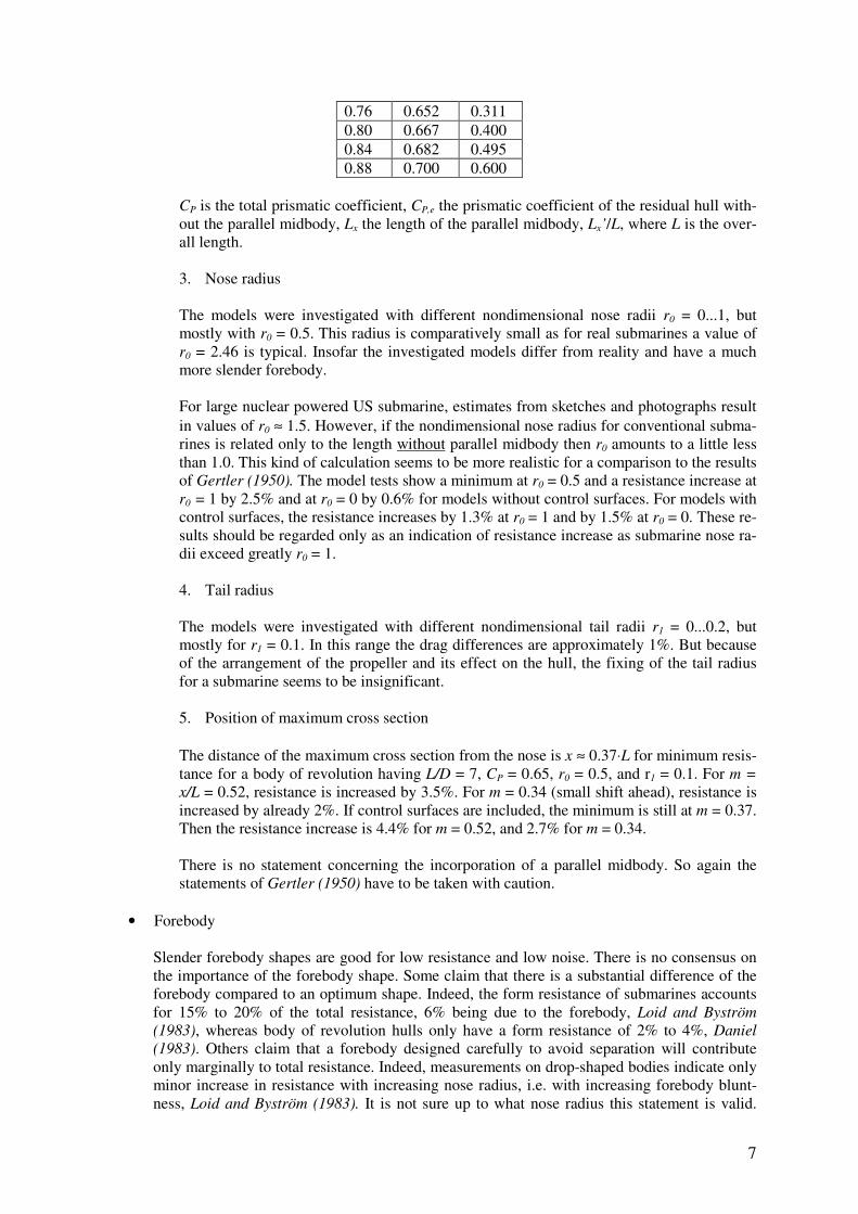
Special care is required in the detailed shaping of the lines for greater CP values. The fol-lowing table lists favourable combinations of CP, CP,e and Lx, Arentzen and Mandel

(1960):

CP CP,e Lx’ 0.60 0.600 0.000 0.64 0.612 0.068 0.68 0.625 0.143 0.70 0.632 0.185 0.72 0.638 0.225

7

0.76 0.652 0.311 0.80 0.667 0.400 0.84 0.682 0.495 0.88 0.700 0.600

CP is the total prismatic coefficient, CP,e the prismatic coefficient of the residual hull with-out the parallel midbody, Lx the length of the parallel midbody, Lx’/L, where L is the over-all length.

3. Nose radius

The models were investigated with different nondimensional nose radii r0 = 0...1, but mostly with r0 = 0.5. This radius is comparatively small as for real submarines a value of r0 = 2.46 is typical. Insofar the investigated models differ from reality and have a much more slender forebody.

For large nuclear powered US submarine, estimates from sketches and photographs result in values of r0 ≈ 1.5. However, if the nondimensional nose radius for conventional subma-rines is related only to the length without parallel midbody then r0 amounts to a little less than 1.0. This kind of calculation seems to be more realistic for a comparison to the results of Gertler (1950). The model tests show a minimum at r0 = 0.5 and a resistance increase at r0 = 1 by 2.5% and at r0 = 0 by 0.6% for models without control surfaces. For models with control surfaces, the resistance increases by 1.3% at r0 = 1 and by 1.5% at r0 = 0. These re-sults should be regarded only as an indication of resistance increase as submarine nose ra-dii exceed greatly r0 = 1.

4. Tail radius

The models were investigated with different nondimensional tail radii r1 = 0...0.2, but mostly for r1 = 0.1. In this range the drag differences are approximately 1%. But because of the arrangement of the propeller and its effect on the hull, the fixing of the tail radius for a submarine seems to be insignificant.

5. Position of maximum cross section

The distance of the maximum cross section from the nose is x ≈ 0.37⋅L for minimum resis-tance for a body of revolution having L/D = 7, CP = 0.65, r0 = 0.5, and r1 = 0.1. For m =

x/L = 0.52, resistance is increased by 3.5%. For m = 0.34 (small shift ahead), resistance is increased by already 2%. If control surfaces are included, the minimum is still at m = 0.37. Then the resistance increase is 4.4% for m = 0.52, and 2.7% for m = 0.34.

There is no statement concerning the incorporation of a parallel midbody. So again the statements of Gertler (1950) have to be taken with caution.

• Forebody

Slender forebody shapes are good for low resistance and low noise. There is no consensus on the importance of the forebody shape. Some claim that there is a substantial difference of the forebody compared to an optimum shape. Indeed, the form resistance of submarines accounts for 15% to 20% of the total resistance, 6% being due to the forebody, Loid and Byström

(1983), whereas body of revolution hulls only have a form resistance of 2% to 4%, Daniel

(1983). Others claim that a forebody designed carefully to avoid separation will contribute only marginally to total resistance. Indeed, measurements on drop-shaped bodies indicate only minor increase in resistance with increasing nose radius, i.e. with increasing forebody blunt-ness, Loid and Byström (1983). It is not sure up to what nose radius this statement is valid.

8

Low pressure peaks increase with the shortening of the forebody, but the influence of the nose radius reduces.

In practice, options for optimisation are limited by other design constraints, mainly by the re-quired number of torpedo tubes and by the shape and position of the acoustic sensors. Major low-pressure peaks have to be avoided with regard to the mine threat. Appendages, e.g. sonar domes, may add significantly to the resistance of the submarine if they are not properly inte-grated into the forebody lines.

• Aftbody

The shape of the aftbody cannot be considered in isolation from the propeller as the propeller modifies considerably the flow over the aftbody. The best form for a propelled body is not the best form for a towed body.

For the body in unpropelled condition, a stern cone angle of θ = 20° can be regarded as a limit for flow separation for a parabolic outline of the aftbody or θ = 18° for an aftbody composed from a cone at the stern until a diameter of half maximum breadth is reached and a parabolic transition with the vertex at the cylindrical midbody.

For the submarine in propelled condition, the flow acceleration due to the propeller prevents separation for much higher cone angles. A thicker aftbody is desirable for reasons of weight distribution and space requirements. This adds also to a smaller frictional resistance by a smaller wetted surface due to a better fineness ratio. A cone plus parabola allows a greater fullness of the aftbody and therefore this shape can be regarded as more favourable.

The local radius of the submarine formed by a cone and parabolic transition is given by:

θtan⋅= xb for the cone up to b = R/2 (1)

−−=

2

5.1tan5.01 θR

xRb for the parabolic transition (2)

Model tests at HSVA with two submarine models of identical shape except for the fullness of the aftbodies showed a somewhat higher resistance at maximum speed for the thicker aftbody but a slightly lower delivered power. Related to the total volume also the resistance was less for the submarine with the thicker aftbody. Thus the experience is confirmed that a larger fric-tional wake is beneficial for the propulsion. The model with the thicker aftbody had a top con-tour angle of 22° and a bottom contour angle of 11°. The respective angles for the slender aft-body were 19° and 10°.

• Appendages & hull openings

Attention has to be paid to secure a smooth curvature of the hull surface in the direction of the streamlines as well as to avoid obstacles as far as possible. If certain appendages (e.g. bollards, capstan heads, railings, etc.) are absolutely necessary they have to be streamlined, removable or made to be able to drop flush with the surface. A certain amount of hull openings (e.g. flooding and venting holes of the main ballast tanks and the free flooding spaces) cannot be avoided. But care should be taken to shape these openings as small and favourable as possible, since a slotted opening has a resistance 4 to 5 times as great as the frictional resistance of a plate of the same size.

Hull openings and surface roughness may cancel the benefits of an optimum shaping. They have to be kept as small as possible and the surface of the shell should be kept as smooth as possible throughout service.

9

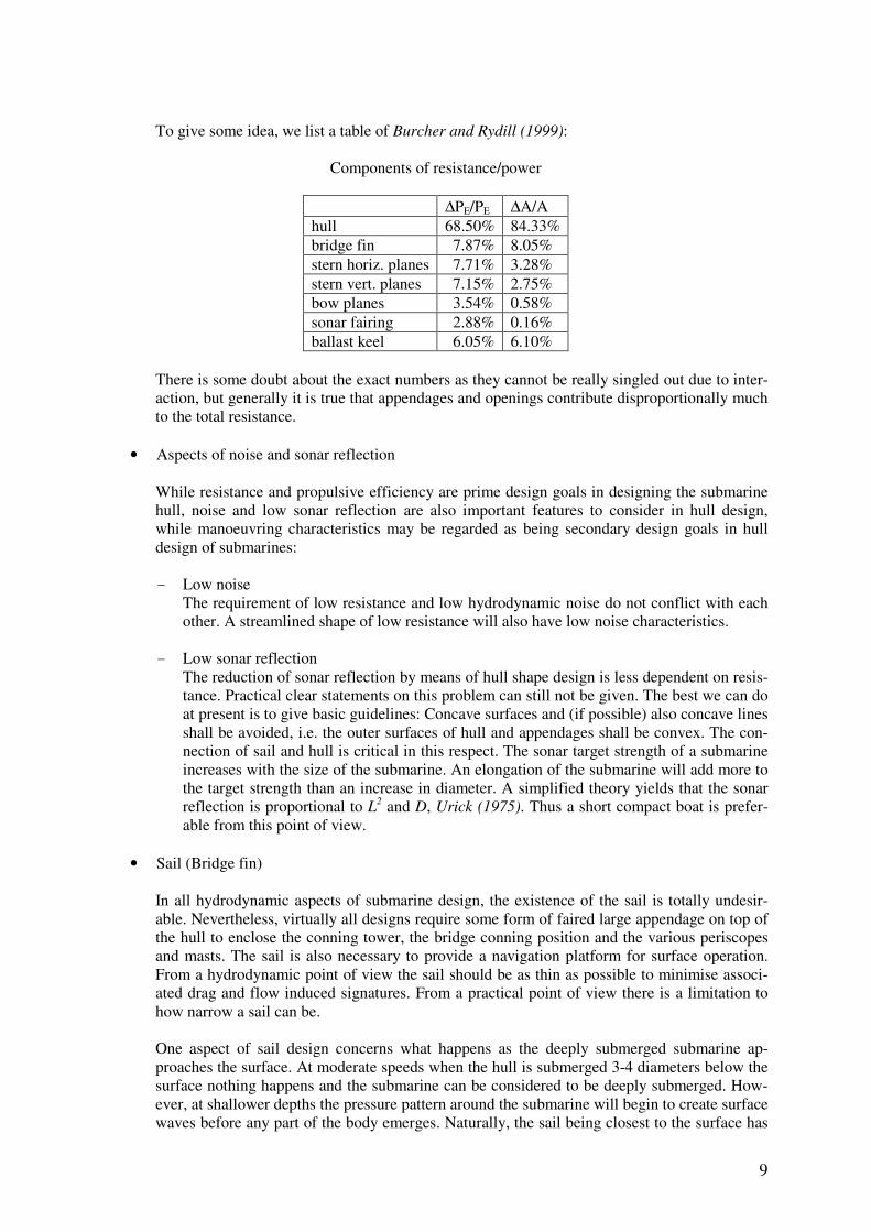
To give some idea, we list a table of Burcher and Rydill (1999):

Components of resistance/power

∆PE/PE ∆A/A hull 68.50% 84.33% bridge fin 7.87% 8.05% stern horiz. planes 7.71% 3.28% stern vert. planes 7.15% 2.75% bow planes 3.54% 0.58% sonar fairing 2.88% 0.16% ballast keel 6.05% 6.10%

There is some doubt about the exact numbers as they cannot be really singled out due to inter-action, but generally it is true that appendages and openings contribute disproportionally much to the total resistance.

• Aspects of noise and sonar reflection

While resistance and propulsive efficiency are prime design goals in designing the submarine hull, noise and low sonar reflection are also important features to consider in hull design, while manoeuvring characteristics may be regarded as being secondary design goals in hull design of submarines: - Low noise

The requirement of low resistance and low hydrodynamic noise do not conflict with each other. A streamlined shape of low resistance will also have low noise characteristics.

- Low sonar reflection

The reduction of sonar reflection by means of hull shape design is less dependent on resis-tance. Practical clear statements on this problem can still not be given. The best we can do at present is to give basic guidelines: Concave surfaces and (if possible) also concave lines shall be avoided, i.e. the outer surfaces of hull and appendages shall be convex. The con-nection of sail and hull is critical in this respect. The sonar target strength of a submarine increases with the size of the submarine. An elongation of the submarine will add more to the target strength than an increase in diameter. A simplified theory yields that the sonar reflection is proportional to L2 and D, Urick (1975). Thus a short compact boat is prefer-able from this point of view.

• Sail (Bridge fin)

In all hydrodynamic aspects of submarine design, the existence of the sail is totally undesir-able. Nevertheless, virtually all designs require some form of faired large appendage on top of the hull to enclose the conning tower, the bridge conning position and the various periscopes and masts. The sail is also necessary to provide a navigation platform for surface operation. From a hydrodynamic point of view the sail should be as thin as possible to minimise associ-ated drag and flow induced signatures. From a practical point of view there is a limitation to how narrow a sail can be.

One aspect of sail design concerns what happens as the deeply submerged submarine ap-proaches the surface. At moderate speeds when the hull is submerged 3-4 diameters below the surface nothing happens and the submarine can be considered to be deeply submerged. How-ever, at shallower depths the pressure pattern around the submarine will begin to create surface waves before any part of the body emerges. Naturally, the sail being closest to the surface has

10

a strong influence and its wave systems can positively or negatively interfere with the wave system of the hull. Methods of analysing this effect will be discussed in detail later.

Besides flow optimisation, the reduction of target strength has a dominant impact on sail ge-ometry. The ultimate design is to incline the surfaces against the vertical and to almost inte-grate the sail into the hull. This reduces the target strength and the formation of strong horse-shoe vortices. The curvature of the sail leading edge can be optimised to reduce the overall in-terference pressure, thereby eliminating a potential hydrodynamic disturbance source.

2. Hydrodynamic assessment

2.1. Introduction to CFD methods

Computational fluid dynamics (CFD) denotes methods solving one or more differential equations de-scribing flows by using a numerical discretisation scheme. We will discuss the possible choices for equations and numerical techniques separately in the following:

• Basic equations

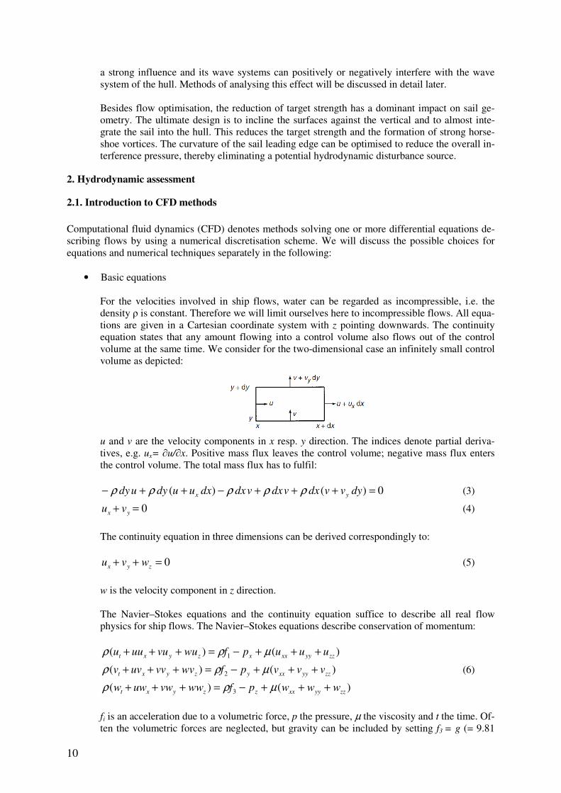
For the velocities involved in ship flows, water can be regarded as incompressible, i.e. the density ρ is constant. Therefore we will limit ourselves here to incompressible flows. All equa-tions are given in a Cartesian coordinate system with z pointing downwards. The continuity equation states that any amount flowing into a control volume also flows out of the control volume at the same time. We consider for the two-dimensional case an infinitely small control volume as depicted:

u and v are the velocity components in x resp. y direction. The indices denote partial deriva-tives, e.g. ux= ∂u/∂x. Positive mass flux leaves the control volume; negative mass flux enters the control volume. The total mass flux has to fulfil:

0)()( =+++−++− dyvvdxvdxvdxdxuudyudy yx ρρρρρ (3)

0=+ yx vu (4)

The continuity equation in three dimensions can be derived correspondingly to:

0=++ zyx wvu (5)

w is the velocity component in z direction.

The Navier–Stokes equations and the continuity equation suffice to describe all real flow physics for ship flows. The Navier–Stokes equations describe conservation of momentum:

)()( 1 zzyyxxxzyxt uuupfwuvuuuu +++−=+++ µρρ

)()( 2 zzyyxxyzyxt vvvpfwvvvuvv +++−=+++ µρρ (6)

)()( 3 zzyyxxzzyxt wwwpfwwvwuww +++−=+++ µρρ

fi is an acceleration due to a volumetric force, p the pressure, µ the viscosity and t the time. Of-ten the volumetric forces are neglected, but gravity can be included by setting f3 = g (= 9.81

11

m/s2) or the propeller action can be modelled by a distribution of volumetric forces f1. The l.h.s. of the Navier–Stokes equations without the time derivative describes convection, the time de-rivative describes the rate of change (‘source term’), and the last term on the r.h.s. describes diffusion.

Navier–Stokes equations and the continuity equation form a system of coupled, non-linear par-tial differential equations. An analytical solution of this system is not possible for ship flows. Neither is a direct numerical solution.

Velocities and pressure may be divided into a time average and a fluctuation part to bring the Navier–Stokes equations closer to a form where a numerical solution is possible. Time averag-ing yields the Reynolds-averaged Navier–Stokes equations (RANSE). u, v, w and p are from now on time averages. u’, v’, w’ denote the fluctuation parts. For unsteady flows (e.g. ma-noeuvring), high-frequency fluctuations are averaged over a chosen time interval (assembly average). This time interval is small compared to the global motions, but large compared to the turbulent fluctuations. The RANSE have a similar form to the Navier–Stokes equations:

)()( 1 zzyyxxxzyxt uuupfwuvuuuu +++−=+++ µρρ )))''()''()''(( zyx wuvuuu ++− ρ

)()( 2 zzyyxxyzyxt vvvpfwvvvuvv +++−=+++ µρρ )))''()''()''(( zyx wvvvvu ++− ρ (7)

)()( 3 zzyyxxzzyxt wwwpfwwvwuww +++−=+++ µρρ )))''()''()''(( zyx wwwvwu ++− ρ

They contain as additional terms the derivatives of the Reynolds stresses:

'''''' wuvuuu ρρρ −−−

'''''' wvvvvu ρρρ −−− (8)

'''''' wwwvwu +−− ρρ

The time-averaging eliminated the turbulent fluctuations in all terms except the Reynolds stresses. The RANSE require a turbulence model that couples the Reynolds stresses to the av-erage velocities.

‘Large-eddy simulations’ (LES) are located between Navier–Stokes equations and RANSE. LES let the grid resolve the large vortices in the turbulence directly and only model the smaller turbulence structures. Depending on what is considered ‘small’, this method lies closer to RANSE or actual Navier–Stokes equations. So far few researchers have attempted LES computations for ship flows and the grid resolution was often too coarse to allow any real pro-gress compared to RANSE solutions. Bensow and Fureby (2007) presented LES applications to submarine hulls in manoeuvring. Many experts see LES as a key technology for maritime CFD applications that may drift into industry application within the next two decades.

Neglecting viscosity - and thus all turbulence effects - turns the Navier-Stokes equations into the Euler equations which still have to be solved together with the continuity equations:

)()( 1 zzyyxxxzyxt uuupfwuvuuuu +++−=+++ µρρ

)()( 2 zzyyxxyzyxt vvvpfwvvvuvv +++−=+++ µρρ (9)

)()( 3 zzyyxxzzyxt wwwpfwwvwuww +++−=+++ µρρ

A further simplification is the assumption of irrotational flow:

12

0

/

/

/

=×

∂∂

∂∂

∂∂

=×∇ v

z

y

x

vrr

(10)

A flow that is irrotational, inviscid and incompressible is called potential flow. In potential flows the components of the velocity vector are no longer independent from each other. They are coupled by the potential φ. The derivative of the potential in arbitrary direction gives the velocity component in this direction:

φ∇=

=

w

v

u

vr

(11)

Three unknowns (the velocity components) are thus reduced to one unknown (the potential). This leads to a considerable simplification of the computation.

The continuity equation simplifies to Laplace’s equation for potential flow:

0=++=∆ zzyyxx φφφφ (12)

If the volumetric forces are limited to gravity forces, the Euler equations can be integrated yielding Bernoulli’s equation:

( ) .1

2

1 2constpgzt =+−∇+

ρφφ (13)

The Laplace equation is sufficient to solve for the unknown velocities. The Laplace equation is linear. This offers the big advantage of combining elementary solutions (so-called sources, sinks, dipoles, vortices) to arbitrarily complex solutions. Potential flow codes are widely used in hull and propeller design.

• Basic CFD techniques

CFD comprises methods that solve the basic field equations subject to boundary conditions by approaches involving a large number of (mathematically simple) elements. These approaches lead automatically to a large number of unknowns. Basic CFD techniques are:

- Boundary Element Methods (BEM)

BEM (or panel methods) are used for potential flows. For potential flows, the integrals over the whole fluid domain can be transformed to integrals over the boundaries of the fluid domain. The step from space (3-d) to surface (2-d) simplifies grid generation and often accelerates computations. Panel methods divide the surface of a ship (and often part of the surrounding water surface) into discrete elements (panels). Fundamentals of BEM can be found in, e.g., Hess (1986, 1990).

- Finite Element Methods (FEM)

FEM dominate structural analysis. For ship hydrodynamics they play only a minor role. Unlike in structural analysis, the elementary functions cannot be used also as weight functions to determine the weighted error integrals (residuals) in a Galerkin method. This reduces the elegance of the method considerably.

- Finite Difference Methods (FDM)

FDM discretise (like FEM) the whole fluid domain. The derivatives in the field equa-tions are approximated by finite differences. Discretisation errors can lead to a viola-tion of conservation of mass or momentum, i.e. in the course of a simulation the

13

amount of water might diminish continuously. While FDM lose popularity and finite volume methods (FVM) gain popularity, FDM give in many cases results of compara-ble quality.

- Finite Volume Methods (FVM)

FVM also employ finite differences for the spatial and temporal discretisation. How-ever, they integrate the equations for mass and momentum conservation over the indi-vidual cell before variables are approximated by values at the cell centres. This en-sures conservativeness, i.e. mass and momentum are conserved because errors at the exit face of a cell cancel with errors at the entry face of the neighbour cell. Most commercial RANSE solvers today are based on FVM. Fundamentals of FVM can be found in Ferziger and Peric (1996).

FEM, FDM, and FVM are called 'field methods', because they all discretise the whole fluid domain (field) as opposed to BEM which just discretise the boundaries.

2.2. Introduction to model tests

2.2.1. Similarity laws

Model tests are still essential in the design process. Before we discuss experimental techniques, we need to review similarity laws fundamental to model tests. See Bertram (2011) for more details. Model tests should be performed such that model and full-scale ship exhibit similar behaviour, i.e. the results for the model can be transferred to full scale by a proportionality factor. We indicate in the following the full-scale ship by the index s and the model by the index m. We distinguish between

• geometrical similarity • kinematical similarity • dynamical similarity

Geometrical similarity means that the ratio of a full-scale ‘length’ (length, width, draft etc.) Ls to a model-scale ‘length’ Lm is constant, namely the model scale λ:

ms LL ⋅= λ (14)

Correspondingly we get for areas and volumes: As=λ2⋅Am; ∇s=λ3⋅∇m. In essence, the model then ‘ap-pears’ to be the same as the full-scale ship. However, in microscopic dimensions, e.g. for surface roughness, geometrical similarity is not obtained. Kinematic similarity means that the ratio of full-scale times ts to model-scale times tm is constant,

namely the kinematic model scale τ: ms tt ⋅= τ .

Dynamical similarity means that the ratio of all forces acting on the full-scale ship to the correspond-

ing forces acting on the model is constant, namely the dynamical model scale: ms FF ⋅= κ .

Forces acting on the ship encompass inertial forces, gravity forces, and frictional forces. Hydrody-namic forces are often described by a coefficient c as follows:

AVcF ⋅⋅⋅= 2

2

1ρ (15)

ρ is the density of water, A the reference area (e.g. wetted surface in calm water), V the reference speed (e.g. ship speed). The force coefficient c is usually assumed to be constant for both ship and model. For dynamical similarity of inertial and gravity forces, we need to have:

14

m

m

s

s

m

s

L

V

L

V

V

V=→= λ (16)

It is customary to use a nondimensional ratio of velocity and square root of length, using g= 9.81 m/s2. This yields the Froude number:

Lg

VFn

⋅= (17)

For the same Froude number, the wave pattern in model and full scale are geometrically similar. This is only true for waves of small amplitude where gravity is the only relevant physical mechanism. Breaking waves and splashes involve another physical mechanism (e.g. surface tension) and do not scale so easily. For dynamical similarity of inertial and frictional forces, we need to have:

m

mm

s

ss LVLV

νν

⋅=

⋅ (18)

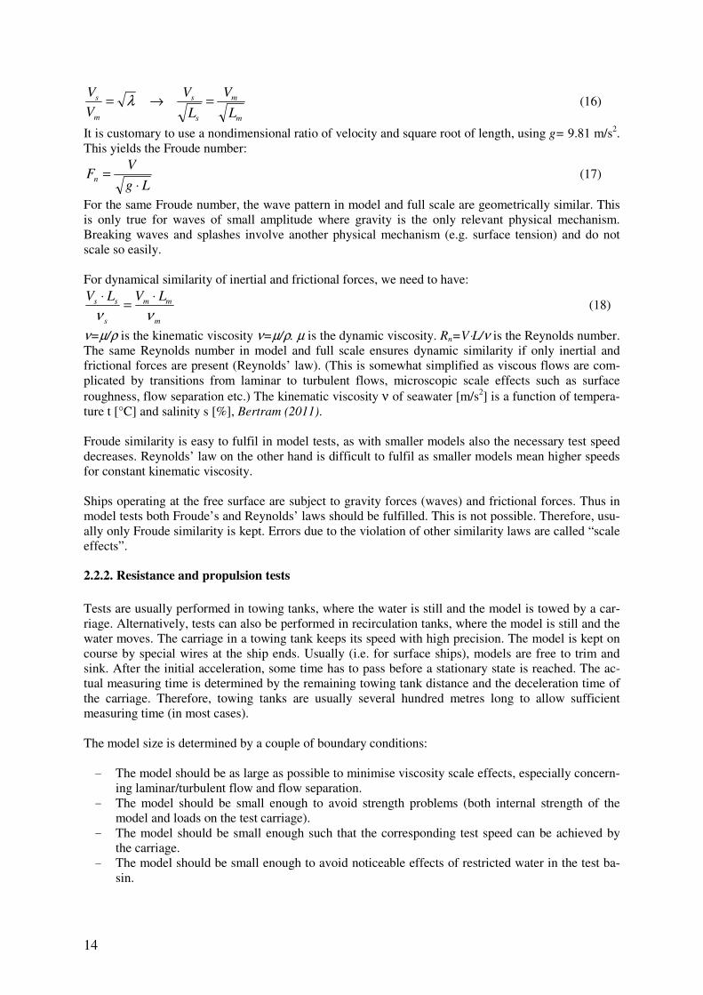
ν=µ/ρ is the kinematic viscosity ν=µ/ρ. µ is the dynamic viscosity. Rn=V⋅L/ν is the Reynolds number. The same Reynolds number in model and full scale ensures dynamic similarity if only inertial and frictional forces are present (Reynolds’ law). (This is somewhat simplified as viscous flows are com-plicated by transitions from laminar to turbulent flows, microscopic scale effects such as surface roughness, flow separation etc.) The kinematic viscosity ν of seawater [m/s2] is a function of tempera-ture t [°C] and salinity s [%], Bertram (2011). Froude similarity is easy to fulfil in model tests, as with smaller models also the necessary test speed decreases. Reynolds’ law on the other hand is difficult to fulfil as smaller models mean higher speeds for constant kinematic viscosity. Ships operating at the free surface are subject to gravity forces (waves) and frictional forces. Thus in model tests both Froude’s and Reynolds’ laws should be fulfilled. This is not possible. Therefore, usu-ally only Froude similarity is kept. Errors due to the violation of other similarity laws are called “scale effects”.

2.2.2. Resistance and propulsion tests

Tests are usually performed in towing tanks, where the water is still and the model is towed by a car-riage. Alternatively, tests can also be performed in recirculation tanks, where the model is still and the water moves. The carriage in a towing tank keeps its speed with high precision. The model is kept on course by special wires at the ship ends. Usually (i.e. for surface ships), models are free to trim and sink. After the initial acceleration, some time has to pass before a stationary state is reached. The ac-tual measuring time is determined by the remaining towing tank distance and the deceleration time of the carriage. Therefore, towing tanks are usually several hundred metres long to allow sufficient measuring time (in most cases). The model size is determined by a couple of boundary conditions: - The model should be as large as possible to minimise viscosity scale effects, especially concern-

ing laminar/turbulent flow and flow separation. - The model should be small enough to avoid strength problems (both internal strength of the

model and loads on the test carriage). - The model should be small enough such that the corresponding test speed can be achieved by

the carriage. - The model should be small enough to avoid noticeable effects of restricted water in the test ba-

sin.

15

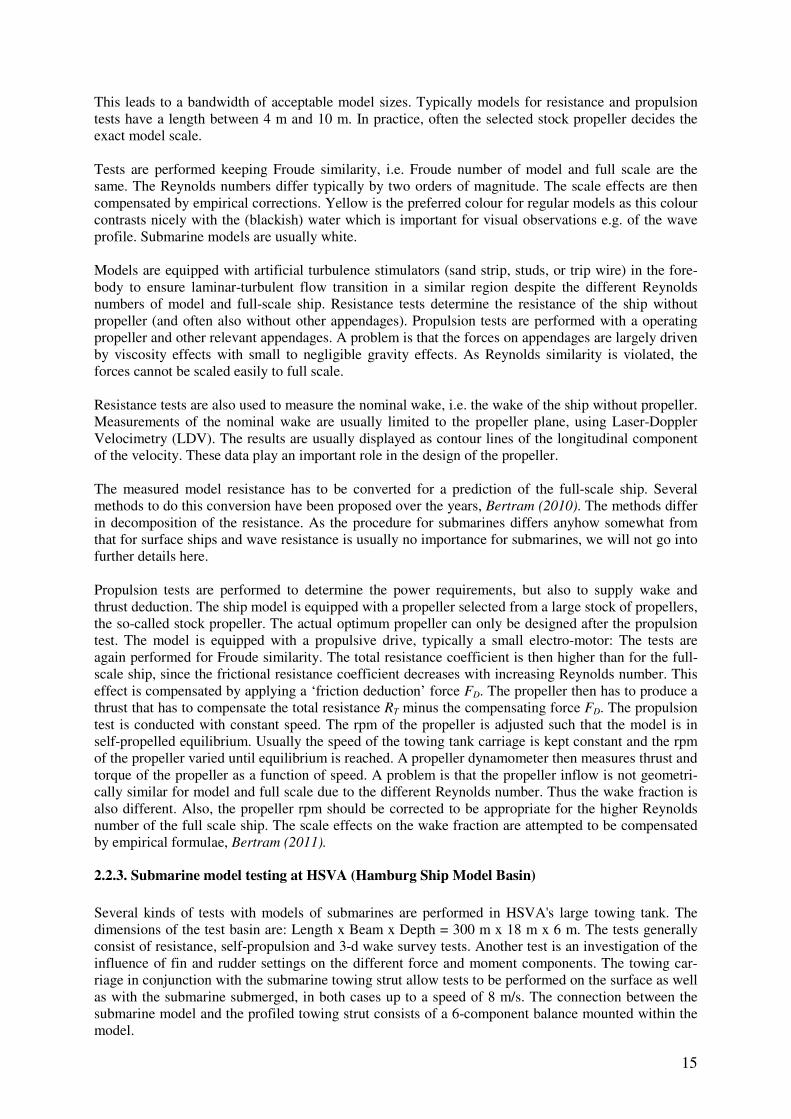
This leads to a bandwidth of acceptable model sizes. Typically models for resistance and propulsion tests have a length between 4 m and 10 m. In practice, often the selected stock propeller decides the exact model scale. Tests are performed keeping Froude similarity, i.e. Froude number of model and full scale are the same. The Reynolds numbers differ typically by two orders of magnitude. The scale effects are then compensated by empirical corrections. Yellow is the preferred colour for regular models as this colour contrasts nicely with the (blackish) water which is important for visual observations e.g. of the wave profile. Submarine models are usually white. Models are equipped with artificial turbulence stimulators (sand strip, studs, or trip wire) in the fore-body to ensure laminar-turbulent flow transition in a similar region despite the different Reynolds numbers of model and full-scale ship. Resistance tests determine the resistance of the ship without propeller (and often also without other appendages). Propulsion tests are performed with a operating propeller and other relevant appendages. A problem is that the forces on appendages are largely driven by viscosity effects with small to negligible gravity effects. As Reynolds similarity is violated, the forces cannot be scaled easily to full scale. Resistance tests are also used to measure the nominal wake, i.e. the wake of the ship without propeller. Measurements of the nominal wake are usually limited to the propeller plane, using Laser-Doppler Velocimetry (LDV). The results are usually displayed as contour lines of the longitudinal component of the velocity. These data play an important role in the design of the propeller. The measured model resistance has to be converted for a prediction of the full-scale ship. Several methods to do this conversion have been proposed over the years, Bertram (2010). The methods differ in decomposition of the resistance. As the procedure for submarines differs anyhow somewhat from that for surface ships and wave resistance is usually no importance for submarines, we will not go into further details here. Propulsion tests are performed to determine the power requirements, but also to supply wake and thrust deduction. The ship model is equipped with a propeller selected from a large stock of propellers, the so-called stock propeller. The actual optimum propeller can only be designed after the propulsion test. The model is equipped with a propulsive drive, typically a small electro-motor: The tests are again performed for Froude similarity. The total resistance coefficient is then higher than for the full-scale ship, since the frictional resistance coefficient decreases with increasing Reynolds number. This effect is compensated by applying a ‘friction deduction’ force FD. The propeller then has to produce a thrust that has to compensate the total resistance RT minus the compensating force FD. The propulsion test is conducted with constant speed. The rpm of the propeller is adjusted such that the model is in self-propelled equilibrium. Usually the speed of the towing tank carriage is kept constant and the rpm of the propeller varied until equilibrium is reached. A propeller dynamometer then measures thrust and torque of the propeller as a function of speed. A problem is that the propeller inflow is not geometri-cally similar for model and full scale due to the different Reynolds number. Thus the wake fraction is also different. Also, the propeller rpm should be corrected to be appropriate for the higher Reynolds number of the full scale ship. The scale effects on the wake fraction are attempted to be compensated by empirical formulae, Bertram (2011).

2.2.3. Submarine model testing at HSVA (Hamburg Ship Model Basin)

Several kinds of tests with models of submarines are performed in HSVA's large towing tank. The dimensions of the test basin are: Length x Beam x Depth = 300 m x 18 m x 6 m. The tests generally consist of resistance, self-propulsion and 3-d wake survey tests. Another test is an investigation of the influence of fin and rudder settings on the different force and moment components. The towing car-riage in conjunction with the submarine towing strut allow tests to be performed on the surface as well as with the submarine submerged, in both cases up to a speed of 8 m/s. The connection between the submarine model and the profiled towing strut consists of a 6-component balance mounted within the model.

16

The main application of resistance and propulsion tests is for submerged condition. In this case the submarine trim and submergence is always fixed. Prior to performing the tests, the 6-component bal-ance (with strain gauges) must be calibrated. The balance records the hydrodynamic forces and mo-ments acting on the hull. Special care is taken when placing the model in the water, adjusting it to towing depth (usually between 2.1 m to 2.5 m) and installing ballast weights. These weights are neces-sary to compensate for the hydrostatic lift of the submarine model and also to ensure a homogenous load distribution for the individual measuring balance components. For the application of the ballast weights the use of a diver is necessary during the set-up procedure. The model can be adjusted to trim and drift angles up to ±5°. The models are in general manufactured to such a scale that the model length is between 5 and 6 m. FRP is the material of choice as it is easier to get neutral buoyancy with such models. For turbulence stimulation, two rows of studs (diameters 2 mm, height 4 mm, being spaced 20 mm from each other) are fitted 100 mm and 300 mm from the bow. Another row of studs is placed 100 mm behind the lead-ing edge of the bridge fin. For the first self-propulsion tests a stock propeller is used. The propeller shaft is driven by an electric motor. DC is used to enable fine adjustment of the revolutions. The shaft revolutions are recorded by an electronic counter (photo-electric). The propeller's thrust and torque is recorded by a shaft dyna-mometer. The towing carriage is electronically controlled in such a way that after a short acceleration phase the selected speed is kept constant during the actual measuring phase until deceleration to stand-still at end of the tank commences. A computerised data recording and processing system is installed in the carriage.

• Resistance test

The tests are carried out for different speeds. During the test, the resistance is directly meas-ured in dependence on the carriage's speed and analysed accordingly. Despite extensive turbu-lence stimulators, it is not possible to create fully turbulent flow in the lower speed range for submarine models. As a result, the resistance is under-predicted for lower speeds. For high speeds, the possible submergence depth becomes increasingly insufficient and a wave system is created at the free surface. This results in an increasing wave resistance contribution which distorts the results. Resistance is thus over-predicted for high speeds.

For medium speeds, these distorting effects play no or only a minor role. This can be seen in a comparison of the frictional resistance coefficient CF (according to ITTC'57) and the total re-sistance coefficient CT as determined from the resistance tests, both plotted as a function of the Reynolds number. The difference between CT and CF, and thus the CR (residual resistance) value, is rather constant in the middle speed range. Based on this insight, the standard proce-dure for submarine resistance tests is as follows: The speed range for the test itself can be smaller than the speed range to be given in the prediction, but covers at least the middle range in which the residual resistance coefficient is more or less constant. The constant CR value as determined from the resistance test results for the middle speed range is used in the evaluation for the entire speed range. This procedure minimises the distorting effects of laminar flow at lower speeds and wave-making resistance at higher speeds. The conversion of the total resis-tance to full scale is then made as usual.

• Self-propulsion tests

The same effects concerning laminar flow and wave appear also in propulsion tests. Here, a correction is not straightforward. Therefore, propulsion tests are usually conducted only for the medium speed range.

17

The exact propeller rpm are determined as follows: The increased surface friction of the model due to the lower Reynolds number (compared to full scale) is calculated:

)(2

1 2AFsFmmmmD cccSVF −−⋅⋅⋅= ρ (19)

This additional model resistance has to be compensated by a towing force produced by the car-riage. For surface ship models which are free to trim and sink this can be easily achieved by a weight via a string. For the rigidly fixed submarine, another method has to be used to adjust the correct propeller loading. The model is run at constant speed but at different propeller rpm (load variation tests). For each rpm the propeller thrust, torque and rpm are measured in addi-tion to the carriage speed and force and moment components. Based on the measured data for a given speed, the self-propulsion point of the submarine (rpm, thrust and torque) is deter-mined by interpolation. Here the friction correction is taken into account when considering the x-component force. From this data, the resistance test data and the propeller open-water data, the following propulsive coefficients are determined:

- thrust deduction fraction t - wake fraction w - relative rotative efficiency ηR

These coefficients are taken to be constant over the entire speed range, and serve as a basis for the calculation of the full scale power prediction.

• Tests to determine the neutral level flight

For submerged condition it is important to know the trim and the hydroplane angles at which the submarine can operate at all speeds without trimming and compensating. The respective test is performed first of all to run all other tests with the model set at neutral angles, i.e. the trim angle and the sternplane angle. Modern practice is to determine the sternplane angle in such a way that fixed and movable portions form a straight line because this will provide a minimum resistance. For this purpose the fixed and movable portions of the model's stern-planes are connected to each other and mounted rotatably on the sternplane shaft. The speed of the model should be as high as possible for Reynolds similarity. However, wave-making limits the maximum possible speed. The propeller rpm are set to the predetermined approximate value and by means of the force necessary to compensate for the increased surface friction of the model the exact propeller rpm are determined. Then for a series of sternplane assembly angles (which are assumed to be near the neutral angle) the model is towed at several trim an-gles (equal to angles of attack in this case). Vertical forces and pitching moments are plotted against the trim angle with the sternplane as parameter or vice versa. Subsequently the trim and sternplane angles for zero force and moment are plotted against each other. The intersec-tion of the resulting curves for force and moment indicate the neutral angle. According to the obtained angle of the sternplane assembly, the fixed fin is built in.

• Tests for lift forces and moments on hull

If no planar motion investigations are performed, static state tests are made in the towing tank to determine lift forces and moments arising from various angles of attack and various drift angles as well as from sternplane, rudder and bowplane deflections. The model is towed at a constant speed with the respective hull inclination and control surfaces set to certain selected angles. The forces and moments are then measured. The forces and moments refer to the sub-marine as a whole, i.e. the local forces on control surfaces are not measured. These would be quite wrong due to scale effects.

• Flow visualisation

18

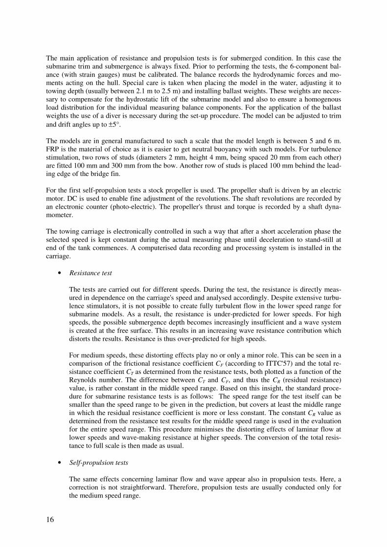
Flow visualisation tests are made in order to show the proper flow over the hull and the ap-pendages. Irregularities such as flow separation and generation of eddies can be detected and subsequently the hull shape may be altered. Different methods are used. We prefer paint tests: Stripes of paint are applied to hull and appendages normal to the direction of flow in certain longitudinal distances, so that the paint can be distributed by the flow over each distance. Im-mediately after applying the paint, the model is immersed into the tank water and towed at a predetermined speed. After lifting the model from the water, the pattern of the flow at the hull can be observed and photographed. The appropriate viscosity of the paint depends on the tem-perature of the tank water, on the speed and on the time spent between applying the paint and towing the model.

Another common method is to attach tufts of thread to the skin. When the model is towed, the threads show the direction of flow. This can be recorded either by an underwater video camera or by photographs. Of course, this method is much more expensive than the paint test espe-cially if the whole surface of the hull and the appendages is to be covered. On the other hand, it is possible to visualise also the flow at some distance away from the hull and to visualise un-steady flows. In practice, the tufts are usually attached only at critical points were flow separa-tion is likely to occur. This keeps expenditure of time and money within reasonable limits.

2.3. Flow analysis on the sonar part

The noise radiated by the submarine is one of the main causes of its vulnerability. The higher the tacti-cal speed is, the more the designer must pay attention to flow induced noise. Flow generated noise must be kept small particularly near the submarine's own sonar systems. Therefore the external hull shape is designed to keep acoustic signature (due to flow perturbations) low, Bovis (1988). Both the hull and appendages may contribute to flow noise generation. Part is due to directly radiated flow noise, part is due to inhomogenities in the submarines wake at the propeller, triggering vibrations and other flow fluctuations. It is important to understand the mechanism of the flow noise generation to derive guidelines in shape design avoiding undue noise generation. Since water is a viscous fluid, a boundary layer is formed inside which the flow velocity grows from 0 at the hull to roughly the submarine's speed (in a ship-fixed coordinate system). This boundary layer is very thin at the bow and grows to 20-50 cm at the aft part, depending on the speed and length of the submarine. At the very beginning, the boundary layer is laminar, i.e. very regular and quiet. At some distance from the bow, small vortices and irregularities in the flow grow, turning the flow eventually into a turbulent flow. This is the laminar-turbulent transition. The location of this transition depends on speed and shape of the hull. Downstream of the transition, the flow remains fully turbulent. A small part of the flow induced noise is directly radiated by the velocity fluctuations in the turbulent boundary layer. The power of this radiation is proportional to U5, where U is the submarine's speed. Therefore, this component of the radiated noise becomes significant at high speeds. It is broadband noise. There is not very much the designer can do about this component except trying to keep laminar flow as long as possible. This in turn is difficult due to other design restrictions. A much more important source of noise in relation with the turbulent boundary layer, even at low speed, are flow-induced vibrations. These are due to hydro-elastic coupling with the fluctuating pres-sure in the turbulent boundary layer exciting non-rigid structures in the hull. If the frequency of the flow fluctuations is near one of the natural frequencies of a structure, this part of the submarine is ex-cited to vibrate relatively strongly and generates noise. This is important for radiated noise, as well as for self-noise (where the sonar is concerned). Due to the hydro-elastic coupling this noise is narrow-banded. A particular kind of hydro-elastic coupling occurs when the turbulent boundary layer flows over a cavity (e.g. ballast tank opening). Here natural frequencies of the cavity may be excited generat-ing again radiated and self-noise. In principle, the same problem in principle, but often more severe, appears for appendages. The vortex and turbulence generation make the propeller wake inhomogeneous. The velocity fluctuations induced

19

by the wake on each propeller blade generate lift fluctuations and therefore thrust and torque fluctua-tions. These are transmitted via the propeller shaft to the hull. These pressure fluctuations are the source of low-frequency noise radiated both by the propeller and the hull. Higher harmonics may be dominant. We can give only some guidelines to design hull and appendages with respect to acoustic aspects. Generally the body should be streamlined. Good resistance characteristics often mean also good acoustic characteristics. A streamlined form avoids flow separation and wake perturbations upstream of the propeller. This means a smooth transition between forebody, middle-body and aftbody. The cone angle of the aftbody should be less than 25° to prevent flow separation. In the forebody a design compromise between torpedo tubes and sonar dome has to be found. Experi-ence with various submarine designs has shown that good sonar performance is difficult to achieve with a non-axisymmetric bow. Low self-noise on the sonar dome at the bow implies an axisymmetric bow, allowing the laminar-turbulent transition downstream of the sonar array. CFD can support the design of the bow, particularly with respect to the location of the sonar regarding the transition. The requirement for longer range and lower frequency sonars has led to the development of flank ar-ray sonars (FAS) which demand both length and depth. Essentially the whole of the submarine hull serves as platform for the FAS. If the pressure hull forms the outer boundary of the hull, the FAS has to be mounted outside the hull. This results in a bulge on each side of the hull where the array is fitted. This bulge adds resistance, but also disturbs the flow on the otherwise smooth hull. Turbulent noise thereby generated interferes and reduces the sonar effectiveness. Thus FAS should be smoothed as much as possible into the hull. The FAS should be aligned with the flow direction as much as possible, but changing operational conditions make this impossible to achieve for all conditions. General de-sign guidance is that the longitudinal ends should be tapered into the hull. No further simple design rules can be given. CFD allows more detailed investigations, but also experiments with models in dedicated hydro-acoustic tunnels as HSVA’s HYKAT can support design of the array systems. The size of the appendages, particularly, the sail should be minimised to minimise drag and wake dis-turbance. However, the size is usually dictated by the function of the appendages. Thus a thin stream-lined sail with proper transitions between sail and hull is the best we can do (at present) to minimise flow-induced vibrations and wake perturbations.

3. Hull-appendages interference

3.1. Analysis methods for fins in uniform flow

For foils, analytical-numerical computations are standard in design practice for many years. Typically inviscid methods (based on the boundary element approach or vortex-lattice approach) are used in design. CFD has gained increasingly in importance and is now a serious option for rudder design for ships and control surface design for submarines. Inviscid methods are fast and quite accurate for smaller angles of attack, but cannot predict stall and maximum lift. RANSE solvers can model also stall and can analyse the foil in the boundary of the hull. The main individual computational ap-proaches for foils are (ranked in increasing complexity):

• Lifting surface methods

The lifting surface model describes the inviscid flow about a plate (centre plane), satisfy-ing the Kutta condition (smooth flow at the trailing edge). The flow is determined as a su-perposition of horseshoe vortices.

• Lifting body methods

A foil with finite thickness generates larger lift forces than a plate. This can be taken into account in different ways, typically by arranging vortices on the foil on both sides, alterna-

20

tively by arranging source panels on the hull and a vortex distribution on the centre plane. For rudders, lifting surface or lifting body theory is the method of choice for angles of at-tack where no stall is expected to occur. Beyond the stall angle, only RANSE methods may be used.

• Field methods

Viscous CFD simulations for rudders appeared in the 1990s as research applications and by the year 2000 also as practical design aids. RANSE solvers are by now used regularly as design tool for rudders and other control fins on ships and submarines.

3.2. Interaction of hull and foils

For foils in infinite flow (2-d or 3-d), we can resort to many systematic experiments and also relatively simple computational methods to determine lift and drag coefficients, respectively pressure distribu-tions. However, the flow around the foils changes due to the hull and the flow at the hull changes due to the foil. This mutual interference is significant particularly for the performance evaluation of the hydroplanes. The interference effects may here reach a comparable order of magnitude as the forces on the foil alone. Some empirical data, curves, and simple estimation formulae exist. While not as extensive as for foils alone, we have sufficient material to be comfortable in design. For submarines, we refer usually to data on foils on cylinders and cones, developed for aerospace industry, Schlichting

and Truckenbrodt (1979), Ferrari (1957), Lawrence and Flax (1954). The hull affects the foil forces in two ways:

• Near the hull the boundary layer reduces the velocity. Note that the boundary layer thick-ness may reach values of 0.2-0.5 m.

• The hull changes the local flow direction (angle of attack) and inflow velocity for the foil sections.

For foils of large aspect ratio (e.g. hydroplanes on the sail), the lift coefficients on the foil hardly differ for small and moderate angles of attack. However, the foils stall earlier. This can be explained by the disturbed flow on the suction side of the foils, Schlichting and Truckenbrodt (1979). Thus the lift on the foil collapses close to the hull for larger angles of attack, Fig.2. This has been verified quantita-tively in extensive German wind tunnel tests for foil-hull interaction (dating back to World War II). The influence of a cylindrical hull on a foil has been investigated extensively in experiments and sim-ple potential flow computations. Outside the boundary layer, the local flow velocity near the cylinder is much higher than far away or in uniform flow. (In fact, twice as high directly at the cylinder in an ideal fluid). Thus the foil experiences spanwise different local angle of attacks. Computations with classical flow theories (e.g. conformal mapping techniques, lifting-line methods) have shown good agreement with experiments (for the simple geometries investigated and small angles of attack). Thus systematic computations with such classical methods have been compiled into curves for fast engi-neering estimates as required in early design. For strongly asymmetric foil configurations (as usually found for the upper and lower vertical hydroplanes at the stern) the classical flow theories are less accurate. Here experiments or advanced CFD simulations are necessary if the flow shall be investi-gated in detail. Trailing vortices from the tips of the sail may affect the aft hydroplanes similarly as trailing vortices from the forward hydroplanes. The danger of trailing vortices from the sail is naturally largest for the top hydroplane in cruciform arrangement. But the vortices may affect the lift produced also on the horizontal aft hydroplanes. The effect may be quite strong. It may increase or decrease the effective-ness of the hydroplanes depending on speed, geometry, etc. CFD is the best tool to analyse the danger and magnitude of the interaction of sail with aft hydroplanes.

21

Fig.2: Wing-body interaction (-•- = foil alone; -o- central foil arrangement on body)

3.3. RANSE simulations for hull-appendage interaction

Flows around appendages, especially foils, feature high Reynolds numbers (Rn = 5⋅107) and are fully turbulent. Therefore RANSE computations give better estimates than potential flow codes. They can capture hull, propeller, rudder interaction including cavitation, e.g. Brehm et al. (2011). In rudder design, often NACA profiles are used. Deviations from these profile shapes are usually mo-tivated by a desire for higher maximum lift coefficients. Experiments of Thieme (1962) showed that some profiles with concave sides give a larger lift maximum which is attained in addition at a lower angle of attack. Lift and drag coefficients and maximum lift angles for these profiles at full scale have only been published for a few cases, Söding (1998). The rudder area is the main design parameter in early rudder design. It is usually selected based on statistical data. The required rudder area is often given in the literature as percentage of the lateral area or a similar parameter (L⋅T). This is dangerous. Bodies with short and high lateral area need other rud-ders than bodies which are long and narrow, although both have the same lateral area. Old design prac-tice of just following experience in selecting the rudder for a new design based on the same percentage of lateral area as for the last design has sometimes resulted in costly re-dimensioning of rudders after the full-scale ship proved to be insufficient. Today’s advanced design philosophy is that it is better to invest more resources in the design phase and avoid such costly “repairs”. The choice of aspect ratio and rudder type is driven largely by structural design considerations. This leaves the profile shape as an element of design freedom for achieving hydrodynamic properties. There are two main categories of profile shapes: - Profiles with straight aft flanks. These profiles are simpler in geometry and thus easier to manu-

facture. Typical representatives are profiles of the NACA series 00 and 643.

22

- Profiles with concave aft flanks and finite width at the end. These are more expensive to manu-facture. Representatives are HSVA profiles MP 73 and 71 and IfS profiles 58 TR and 61 TR.

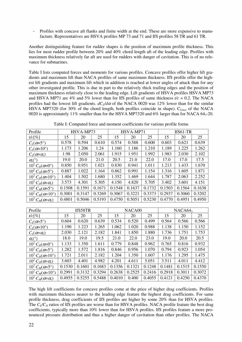
Another distinguishing feature for rudder shapes is the position of maximum profile thickness. This lies for most rudder profile between 20% and 40% chord length aft of the leading edge. Profiles with maximum thickness relatively far aft are used for rudders with danger of cavitation. This is of no rele-vance for submarines. Table I lists computed forces and moments for various profiles. Concave profiles offer higher lift gra-dients and maximum lift than NACA profiles of same maximum thickness. IfS profile offer the high-est lift gradients and maximum lift which in addition is reached at lower angles of attack than for any other investigated profile. This is due in part to the relatively thick trailing edges and the position of maximum thickness relatively close to the leading edge. Lift gradients of HSVA profiles HSVA MP73 and HSVA MP71 are 4% and 5% lower than for IfS profiles of same thickness t/c = 0.2. The NACA profiles had the lowest lift gradients. dCL/dα of the NACA 0020 was 12% lower than for the similar HSVA MP7320 (for 30% of the chord length, both profiles coincide in shape). CLmax of the NACA 0020 is approximately 11% smaller than for the HSVA MP7320 and 6% larger than for NACA 643-20.

Table I: Computed force and moment coefficients for various profile forms

Profile HSVA-MP73 HSVA-MP71 IfS61-TR t/c[%] 15 20 25 15 20 25 15 20 25 CL(α=5°) 0.578 0.594 0.610 0.574 0.588 0.600 0.603 0.621 0.639

CL(α=10°) 1.173 1.206 1.24 1.160 1.186 1.210 1.189 1.225 1.262

CL(α=αs) 1.98 2.050 2.061 1.915 1.951 1.992 1.983 2.030 2.102

αs(°) 19.0 20.0 21.0 20.5 21.0 22.0 17.0 17.0 17.5

102⋅CD(α=0°) 0.850 0.951 1.021 0.830 0.941 1.011 1.213 1.433 1.670

102⋅CD(α=5°) 0.887 1.022 1.164 0.862 0.991 1.154 1.316 1.605 1.871

102⋅CD(α=10°) 1.404 1.502 1.680 1.352 1.469 1.644 1.787 2.063 2.252

102⋅CD(α=αs) 3.573 4.301 5.305 4.150 4.820 5.705 3.402 3.601 4.151

102⋅CM(α=5°) 0.1508 0.1591 0.1671 0.1548 0.1637 0.1732 0.1503 0.1564 0.1638

102⋅CM(α=10°) 0.3001 0.3147 0.3269 0.3067 0.3221 0.3373 0.2937 0.3060 0.3202

102⋅CM(α=αs) 0.4801 0.5046 0.5193 0.4750 0.5051 0.5230 0.4770 0.4951 0.4950 Profile IfS58TR NACA00 NACA643 t/c[%] 15 20 25 15 20 25 15 20 25 CL(α=5°) 0.604 0.620 0.639 0.534 0.520 0.499 0.564 0.566 0.566

CL(α=10°) 1.190 1.223 1.265 1.062 1.020 0.988 1.138 1.150 1.152

CL(α=αs) 2.030 2.121 2.182 1.841 1.850 1.880 1.736 1.751 1.753

αs(°) 18.0 19.0 19.5 21.0 22.0 23.0 19.0 20.0 20.5

102⋅CD(α=0°) 1.133 1.350 1.611 0.779 0.848 0.962 0.765 0.816 0.932

102⋅CD(α=5°) 1.282 1.572 1.816 0.846 0.956 1.070 0.794 0.923 1.054

102⋅CD(α=10°) 1.721 2.011 2.182 1.204 1.350 1.607 1.176 1.295 1.475

102⋅CD(α=αs) 3.603 4.401 4.982 4.201 4.611 5.051 3.511 4.011 4.412

102⋅CM(α=5°) 0.1530 0.1601 0.1683 0.1356 0.1321 0.1248 0.1481 0.1515 0.1550

102⋅CM(α=10°) 0.2991 0.3132 0.3294 0.2638 0.2525 0.2416 0.2918 0.3011 0.3072

102⋅CM(α=αs) 0.4955 0.5255 0.5488 0.4010 0.400 0.4055 0.4121 0.4250 0.4370

The high lift coefficients for concave profiles come at the price of higher drag coefficients. Profiles with maximum thickness nearer to the leading edge feature the highest drag coefficients. For same profile thickness, drag coefficients of IfS profiles are higher by some 20% than for HSVA profiles. The CL/CD ratios of IfS profiles are worse than for HSVA profiles. NACA profile feature the best drag coefficients, typically more than 10% lower than for HSVA profiles. IfS profiles feature a more pro-nounced pressure distribution and thus a higher danger of cavitation than other profiles. The NACA

23

643 is best with respect of cavitation susceptibility. At large angles of attack, profiles with smaller leading edge radius like NACA 643 and HSVA MP 71 feature more pronounced low pressure peaks than other profiles. For concave profiles the change in centre of pressure force with angle of attack is less pronounced than for NACA profiles. El Moctar (2001) gives computed distributions of the pres-sure coefficient Cp for the investigated profiles. In conclusion: - IfS profiles are best in terms of lift, NACA profiles worst. - NACA profiles are best in terms of drag, IfS profiles worst. - HSVA profiles are a good compromise in terms of manoeuvrability and propulsive efficiency.

RANSE simulations can also investigate the effect of rudders interacting with propellers. Modelling the propeller using body forces is sufficient for rudder investigations. For surface ships, rudders oper-ate usually in the propeller slipstream, which increases lift forces by a factor 2 to 3. Submarine aft hydroplanes are usually located some distance upstream of the propeller. Then the propeller effect is much lower. We can attempt to estimate the lift gradient using simpler methods. At HDW, the design tool is a pro-gram based on Bohlmann (1990) combining classical theory with empirical corrections.

4. Analysis methods for snorkels

Michell's thin ship theory, Bertram (2011), can be used to estimate the wave resistance contribution of the snorkel due its high Froude number based on its own length. However, for an analysis of the actual local flow at the snorkel, free-surface RANSE methods have to be used. The many different methods to determine the shape of the free surface can be classified into two groups:

1. Interface-tracking methods which define the free surface as a sharp interface which motion is followed. They use moving grids fitted to the free surface and compute the flow of liquid only. Problems are encountered when the free surface starts folding or when the grid has to be moved along walls of a complicated shape (like a real ship hull geometry).

2. Interface-capturing methods which do not define a sharp interface water/air. The computation is performed on a fixed grid which extends also over the air region. The shape of the free sur-face is determined by finding the cells which are only partially filled with water. This is achieved by either:

a) Marker-and-Cell scheme (MAC):

Some massless particles (markers) are introduced into the water near the free surface at the beginning and followed during the calculation. The scheme can compute com-plex phenomena like wave breaking. However, the computing effort is large since in addition to solving the equations governing the fluid flow, one has to solve the equa-tions describing the movement of a large number of particles.

b) Volume-of-Fluid scheme (VOF):

The transport equation for the void fraction of the water (1 for completely filled, 0 for completely empty cells) is solved (in addition to the usual conservation equations of mass and momentum). The method is more efficient than MAC and can also be ap-plied to breaking of waves. However, the free surface contour is not sharply defined and special techniques had to be developed to obtain an accurate profile with reason-able numbers of cells, e.g. Ferziger and Peric (1999).

The VOF approach is most widely used and works well to capture complex wave breaking.

24

The free surface should be resolved properly. The fundamental wave length λ is related to the Froude number by

22 nFL

πλ

= (20)

At least 20 points per wave lengths should be used for sufficient wave resolution in RANSE computa-tions. The flow around surface-piercing profiles (snorkels and masts) on submarines features high Froude numbers, typically Fn > 2. Unless well designed, these high Froude numbers are often associated with steep, massively breaking waves which cause a significant acoustic signature. The wave making de-pends strongly on the shape of the profile and on the Froude number. The wave breaking causes a mixing of water and air. The flow becomes highly unsteady. Potential flow codes cannot handle breaking waves. Therefore, free-surface RANSE codes are the tool of choice. We then model the flow for the strongly breaking waves as a two-phase flow. We computed the flow around surface-piercing profiles for Fn = 2 and Rn = 3.5 ⋅ 106, El Moctar and

Bertram (2001). These are typical for snorkel masts at snorkelling depth. As the flow is highly un-steady, both port and starboard sides should be modelled even for symmetrical profiles. Typical block-structured grids may consist of 1.5-2 million cells with the majority of the cells clustered near the free-surface to ensure high resolution. Such computations are able to reproduce very realistically the flow around snorkelling masts, Fig. 3. As the leading edge radius increases, the wave height and spray formation increases. Doubling the profile thickness roughly doubles the wave height. Profiles with sharp leading edges produce smaller waves that profiles with rounded leading edges, Fig.3 and Fig.4. The rounded profile is more wetted at the leading edge than at the trailing edge. The sharp profile features a parabolic wetted surface. For all profiles the water sheet above the water line is relatively thin. The wave height may be limited and wave breaking largely suppressed by employing transverse plates on the profile, Fig.5 and Fig.6. These prevent the rise of the thin water sheet at the profile. The width of the transverse plates is decisive for the prevention of spray.

Fig.3: Parabolic strut with sharp edge, side view Fig..4: Cylinder, side view

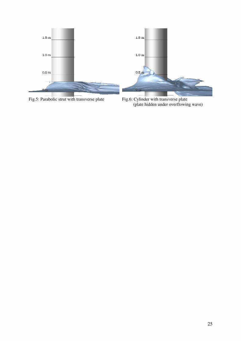
25

Fig.5: Parabolic strut with transverse plate Fig.6: Cylinder with transverse plate

(plate hidden under overflowing wave)

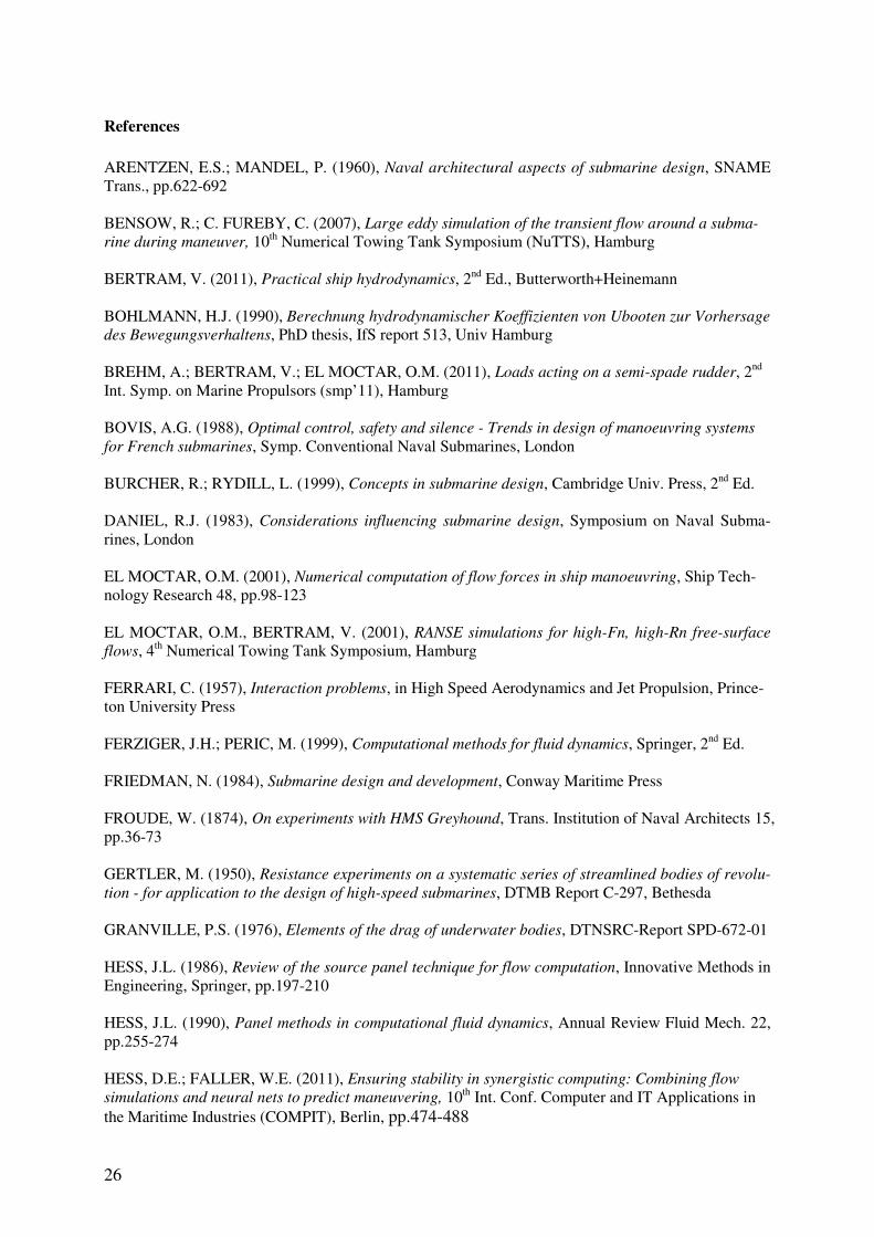
26

References

ARENTZEN, E.S.; MANDEL, P. (1960), Naval architectural aspects of submarine design, SNAME Trans., pp.622-692 BENSOW, R.; C. FUREBY, C. (2007), Large eddy simulation of the transient flow around a subma-

rine during maneuver, 10th Numerical Towing Tank Symposium (NuTTS), Hamburg BERTRAM, V. (2011), Practical ship hydrodynamics, 2nd Ed., Butterworth+Heinemann BOHLMANN, H.J. (1990), Berechnung hydrodynamischer Koeffizienten von Ubooten zur Vorhersage

des Bewegungsverhaltens, PhD thesis, IfS report 513, Univ Hamburg BREHM, A.; BERTRAM, V.; EL MOCTAR, O.M. (2011), Loads acting on a semi-spade rudder, 2nd Int. Symp. on Marine Propulsors (smp’11), Hamburg BOVIS, A.G. (1988), Optimal control, safety and silence - Trends in design of manoeuvring systems

for French submarines, Symp. Conventional Naval Submarines, London BURCHER, R.; RYDILL, L. (1999), Concepts in submarine design, Cambridge Univ. Press, 2nd Ed. DANIEL, R.J. (1983), Considerations influencing submarine design, Symposium on Naval Subma-rines, London EL MOCTAR, O.M. (2001), Numerical computation of flow forces in ship manoeuvring, Ship Tech-nology Research 48, pp.98-123 EL MOCTAR, O.M., BERTRAM, V. (2001), RANSE simulations for high-Fn, high-Rn free-surface

flows, 4th Numerical Towing Tank Symposium, Hamburg FERRARI, C. (1957), Interaction problems, in High Speed Aerodynamics and Jet Propulsion, Prince-ton University Press FERZIGER, J.H.; PERIC, M. (1999), Computational methods for fluid dynamics, Springer, 2nd Ed. FRIEDMAN, N. (1984), Submarine design and development, Conway Maritime Press FROUDE, W. (1874), On experiments with HMS Greyhound, Trans. Institution of Naval Architects 15, pp.36-73 GERTLER, M. (1950), Resistance experiments on a systematic series of streamlined bodies of revolu-

tion - for application to the design of high-speed submarines, DTMB Report C-297, Bethesda GRANVILLE, P.S. (1976), Elements of the drag of underwater bodies, DTNSRC-Report SPD-672-01 HESS, J.L. (1986), Review of the source panel technique for flow computation, Innovative Methods in Engineering, Springer, pp.197-210 HESS, J.L. (1990), Panel methods in computational fluid dynamics, Annual Review Fluid Mech. 22, pp.255-274 HESS, D.E.; FALLER, W.E. (2011), Ensuring stability in synergistic computing: Combining flow

simulations and neural nets to predict maneuvering, 10th Int. Conf. Computer and IT Applications in the Maritime Industries (COMPIT), Berlin, pp.474-488

27

JACKSON, H.A. (1992), Fundamentals of submarine concept design, SNAME Trans., pp.419-448 LANDWEBER, L.; GERTLER, M. (1950), Mathematical formulation of bodies of revolution, DTMB Report 719, Bethesda LAWRENCE, H. R.; FLAX, A.H. (1954), Wing-body interference at subsonic and supersonic speeds

- survey and new developments, J. Aeronaut. Science 21/5, pp. 289-324 LOID, H.P.; BYSTRÖM, L. (1983), Hydrodynamic aspects of the design of the forward and aft bodies

of the submarine, Symposium on Naval Submarines, London MORGAN, W.B.; LIN, W.C. (1998), Predicting ship hydrodynamic performance in today's world, Naval Engineers J., September, pp.91-98 SCHLICHTING, H.; TRUCKENBRODT, E. (1979), Aerodynamics of the Aeroplane, 2nd ed., McGraw Hill SÖDING, H. (1998), Limits of potential theory in rudder flow predictions, Ship Technology Research 45, pp.141-155 THIEME, H. (1962), Zur Formgebung von Schiffsrudern, Jahrbuch schiffbau-technische Gesellschaft, Springer URICK, J.R. (1975), Principles of underwater sound for engineers, McGraw-Hill