Subgrid-scale stresses and their modelling in a turbulent ...

J. Fluid Mech. (1997), vol. 349, pp. 253–293. Printed in the United Kingdom

c© 1997 Cambridge University Press

253

Subgrid-scale stresses and their modelling in aturbulent plane wake

By J O H N O’N E I L† AND C H A R L E S M E N E V E A UDepartment of Mechanical Engineering, The Johns Hopkins University,

Baltimore, MD 21218, USA

(Received 26 December 1996 and in revised form 5 June 1997)

Velocity measurements using hot wires are performed across a high-Reynolds-numberturbulent plane wake, with the aim of studying the subgrid-scale (SGS) stress andits modelling. This quantity is needed to close the filtered Navier–Stokes equationsused for large-eddy simulation (LES) of turbulent flows. Comparisons of variousglobally time-averaged quantities involving the measured and modelled SGS stressare made, with special emphasis on the SGS energy dissipation rate. Experimentalconstraints require the analysis of a one-dimensional surrogate of the SGS dissipation.Broadly, the globally averaged results show that all models considered, namely theSmagorinsky and similarity models, as well as the dynamic Smagorinsky model,approximately reproduce profiles of the surrogate SGS dissipation. Some discrepanciesnear the outer edge of the wake are observed, where the Smagorinsky model slightlyoverpredicts, and the similarity model underpredicts, energy dissipation unless thefiltering scale is about two orders of magnitude smaller than the integral length scale.

A more detailed comparison between real and modelled SGS stresses is achievedby conditional averaging based on particular physical phenomena: (i) the outerintermittency of the wake, and (ii) large-scale coherent structures of the turbulentwake. Thus, the interaction of the subgrid scales with the resolved flow and modelviability can be individually tested in regions where isolated mechanisms such as outerintermittency, vortex stretching, rotation, etc., are dominant. Conditioning on outerintermittency did not help to clarify observed features of the measurements. On theother hand, the large-scale organized structures are found to have a strong impactupon the distribution of surrogate SGS energy dissipation, even at filter scales wellinside the inertial range. The similarity model is able to capture this result, while theSmagorinsky model gives a more uniform (i.e. unrealistic) distribution. Both dynamicSmagorinsky and similarity models reproduce realistic distributions, but only if allfilter levels are contained well inside the inertial range.

1. IntroductionIn large-eddy simulation (LES) of incompressible turbulent flow one seeks solutions

to the filtered Navier–Stokes equations, which requires the subgrid-scale (SGS) stresstensor to be parameterized as function of the resolved velocity field. The SGS tensoris defined according to

τij ≡ uiuj − uiuj , (1)

† Present address: Applied Physics Laboratory, Laurel, MD 20723–6099, USA.

254 J. O’Neil and C. Meneveau

where the tilde represents spatial filtering at a scale ∆. There is a significant body ofliterature on the subject of SGS modelling for LES, e.g. Lilly (1967), Deardorff (1970),Leonard (1974), Kraichnan (1976), Bardina, Ferziger & Reynolds (1980). Comprehen-sive reviews are given in Rogallo & Moin (1984) and, more recently, Lesieur & Metais(1996). The SGS stress τij is a strongly fluctuating variable whose basic propertiesand its relationship with the large scales of the flow must be understood in order toformulate accurate parameterizations.

Given a fully resolved field, the stress can be computed according to its definition,equation (1). This allows SGS stresses computed by filtering fully resolved turbulentfields to be compared with model expressions also evaluated from resolved velocityfields (Clark, Ferziger & Reynolds 1979; Piomelli, Moin & Ferziger 1988). Such apriori studies of SGS modelling have, in the past, concentrated mainly on isotropicturbulence (e.g. Clark et al. 1979; Domaradski, Liu & Brachet 1993), and planarchannel flow (e.g. Piomelli et al. 1988; Hartel et al. 1994). The data were mostlyobtained from direct numerical simulation (DNS) at low Reynolds number (Rλ ∼ 100).Experimental data at higher Reynolds numbers (Rλ ∼ 300) have also been analysedfor the purpose of a priori studies (Liu, Meneveau & Katz 1994). There, two-dimensional particle-image-velocimetry (PIV) measurements were performed in thefar field of a round jet about the jet axis, where the turbulence statistics are notfar from homogeneous. Hot-wire measurements in grid turbulence (Rλ ∼ 150) wereanalysed in Meneveau (1994). Several conclusions have been reached from such apriori studies. Among them has been the realization that on an instantaneous basisthe eddy-viscosity closures do not properly reproduce the real stresses, while thesimilarity models (to be described in detail below) yield more realistic distributions.However, on average the traditional eddy-viscosity models were shown to predict thecorrect rate of energy dissipation in turbulent regions away from walls. Measuredmodel coefficients agreed approximately with traditional values. Quite importantly, itwas shown based on the data that the dynamic procedure (Germano et al. 1991) isable to extract such coefficients from information contained in the resolved scales.

The motivation for the present study is to extend such experimental a priori studiesto include more of the flow complexities typically encountered in turbulent shearflows. In particular, we wish to capture effects of non-homogeneity of flow statisticson properties of the SGS stress. In addition to average spatial non-homogeneity, freeshear flows are characterized by several important features of the instantaneous fields.Among these are outer intermittency, the coexistence of turbulent and irrotationalflow near the shear layer’s edges, and the existence of well-defined large-scale coherentstructures. One would like to know how the real SGS stress τij , the models, and othervariables of interest for LES, respond to the presence of such phenomena at highReynolds numbers. Outer intermittency and large-scale coherent structures are notubiquitous in grid turbulence or fully developed channel flows, and were not availablefrom the PIV data in the inner portion of the far-field jet studied in Liu et al. (1994).

In this study we focus on the planar wake behind a circular cylinder. Measurementswill be performed across a significant portion of the wake, in order to capture thespatial non-homogeneity of this flow. The wake includes the phenomena of outerintermittency, as well as large-scale coherent structures.

A primary issue concerns characterizing fundamental features of the SGS stress andthe applicability of different SGS models. One approach is to examine features of aninstantaneous realization of real and modelled fields, e.g. the SGS dissipation field. Thecomparison can be based on the correlation coefficient of the actual and modelled SGSdissipation across the field. While much can be learned from this approach, partial

Subgrid-scale stresses in a turbulent plane wake 255

agreement of local instantaneous features does not provide a sufficient (or necessary)condition for the proper modelling of the subgrid scales. Another possibility is tocompare mean values, by averaging over very long times. Agreement between certainaveraged quantities can be shown to yield necessary conditions (Meneveau 1994)that a model should reproduce. However, a few average values contain only limitedinformation about the SGS stress. To completely describe turbulence subgrid scalesand the models with statistics requires, in principle, an infinite number of multipointjoint moments.

A more focused comparison based on isolated physical mechanisms can be madeby conditional averaging. As mentioned before, an important phenomenon in thewake is outer intermittency, consisting of the coexistence of turbulent and irrotationalflow, especially at the wake’s edges (Corrsin & Kistler 1955). Another importantphenomenon in this flow is the presence of large-scale coherent structures. Therehas been a large body of work documenting the existence of coherent structure incanonical shear flows, and in the cylinder wake in particular (Hussain & Hayakawa1987; Cantwell 1981). Instead of only calculating global averages, one may usecoherent structure and/or outer intermittency, and conditionally average on thesephenomena to disentangle different large-scale flow phenomena, and study propertiesof the SGS stress and models under such more clearly defined conditions.

In a recent DNS study of channel flow, Piomelli, Yu & Adrian (1996) used theSGS dissipation as a criterion for conditional averaging. Conditional flow structureswere obtained whenever the local SGS dissipation exceeded a positive (or negative)value. They concluded that the interscale energy transfer is highly correlated with thepresence of structures. If this feature is a general property of the relationship betweenlarge-scale coherent structures and SGS dynamics, then the assumption of universalityof small-scale motion may be less justified. We will examine this issue in the contextof the plane wake. In this flow, the most ubiquitous large-scale coherent structures arethe vortices in the Karman-vortex street. They are visible in the near and so-calledintermediate field, maybe up to 30 diameters downstream of the cylinder, even at verylarge Reynolds numbers. Those large-scale structures are characterized by differentregions, ranging from vortex cores to highly strained saddle points.

In order to accurately measure conditional averages, extensive data must be avail-able at every sampling point. This can be accomplished by using traditional thermalanemometry. Of course hot-wire data are severely limited compared to more recentmultidimensional measurement techniques such as particle image velocimetry (Adrian1991; Liu et al. 1994), in the sense that Taylor’s hypothesis must be used, and that itgives only one-dimensional sections through the flow. On the other hand, very longdata records required for converged statistics can be obtained at selected points withhot wires, which is still difficult when using PIV.

Arguably the most important feature of the subgrid-scale stress is how it affectsthe kinetic energy of the resolved field. Thus, energy dissipation arising from theinteractions between subgrid and resolved scales is the main focus of this study. Inorder to more concretely formulate the questions to be addressed, the concept of SGSenergy dissipation is briefly reviewed below. This is followed by a review of the basicmodels to be considered.

1.1. Subgrid-scale energy dissipation

The SGS stress tensor has profound effects on the energetics of the resolved flow field,as can be deduced from the resolved kinetic energy equation (see e.g. Piomelli et al.


1991):

∂ 12q2

∂t+ uj

∂ 12q2

∂xj= − ∂

∂xj

(1

ρpuj + τij ui − 2νuiSij

)− 2νSij Sij + τij Sij + fiui, (2)

where the resolved kinetic energy field is defined as

12q2 ≡ 1

2uiui, (3)

and Sij ≡ 12

(∂ui/∂xj + ∂uj/∂xi

)is the resolved strain-rate tensor. The first term on

the right-hand-side of (2) represents spatial transport, which vanishes on average forhomogeneous flows. The second is direct dissipation due to molecular viscosity. Athigh Reynolds numbers, away from no-slip boundaries, this term is quite small. The

third term, τij Sij , is the so-called SGS dissipation rate, and typically has a negativeaverage value, representing a net drain of resolved kinetic energy into unresolvedmotion. The last term represents energy injection (or extraction) by body forces. Oneconcludes that on average, in the inertial range, the SGS dissipation term representsthe most important effect of the unresolved scales on the evolution of kinetic energyof the resolved field. Therefore, most attention will be devoted to this particularstatistic of the SGS stress.

1.2. Smagorinsky model

Since the inception of LES, the eddy-viscosity model first formulated by Smagorinsky(1963) remains in wide use. The model for the deviatoric part of the stress is

τdij = −2 (CS∆)2∣∣S ∣∣Sij , (4)

where the modulus of the resolved strain rate is∣∣S ∣∣ ≡ (2SmnSmn)1/2. (5)

CS is a dimensionless coefficient. Given the dynamical importance of SGS energydissipation, a strategy to determine, or calibrate, CS from data is to require that theSmagorinsky model reproduces the correct mean SGS dissipation. This leads to

C2S = −

⟨τij Sij

⟩⟨2∆2∣∣S ∣∣SmnSmn⟩ . (6)

The averaging can be ensemble, time, or spatial, depending on specific flow conditions.The coefficient determined by condition (6) (and similar ones for models discussed

later) can be interpreted as follows: using this value in LES is a necessary conditionto reproduce the correct SGS dissipation assuming that the simulation is producing

the correct value of the denominator 2⟨∆2∣∣S ∣∣SmnSmn⟩ (see §3.4 for a more detailed

discussion of this issue).The Smagorinsky model implicitly assumes that the subgrid scales adjust instanta-

neously to changes in the resolved field. By construction, the model is dissipative, andonly allows for forward transfer of energy from the resolved scales to the unresolvedones. Among others, Piomelli et al. (1991) and Liu et al. (1994) have found both ofthese features to be unrealistic.

1.3. Similarity model

The similarity models form a different class of parameterization (Bardina et al. 1980;Liu et al. 1994). They take advantage of the high correlation observed between the


smallest resolved scales and the actual SGS scales, which leads to

τij = CLLij , (7)

where

Lij ≡ uiuj − ui uj . (8)

The overline denotes a second filtering operation, typically at a scale 2∆. Originally(Bardina et al. 1980) this was performed at the same level as the grid filter, ∆, butit was later found to be more appropriate to filter at larger lengths (Liu et al. 1994).By construction, this model assumes that the local stresses at different filter levels arevery similar, so a similarity coefficient CL ∼ O(1) is to be expected. As was done for

the Smagorinsky coefficient, one may contract the SGS stress and model with Sij toform the SGS dissipation, and again solve for the coefficient according to

CL =

⟨τij Sij

⟩⟨LmnSmn

⟩ . (9)

In simulations, the model is typically supplemented with the Smagorinsky model(mixed model) to ensure that mean dissipation of kinetic energy takes place in thesimulation (Zang, Street & Koseff 1993; Vreman, Guerts & Kuerten (1994); etc.). Thesimilarity term then accounts for more local features of the flow, such as backscatter(Liu et al. 1994; Piomelli et al. 1996).

1.4. Dynamic Smagorinsky model

In the traditional Smagorinsky model, the coefficient CS needs to be prescribed apriori. This is a serious drawback since different regions of the flow may requiredifferent coefficient values. For instance, if one is modelling subgrid scales in thepresence of a turbulent/non-turbulent interface, which typically bounds shear flows,one may need to reduce the coefficients in the outer, non-turbulent regions. Germanoet al. (1991) carried the idea of similarity between scales to the next logical step byintroducing the dynamic Smagorinsky model

τdij = −2 (CSD∆)2∣∣S ∣∣Sij , (10)

where the coefficient is obtained from

C2SD =

⟨LijMij

⟩∗⟨MmnMmn

⟩∗ . (11)

Lij was defined in (8), and Mij is defined as

Mij = −2(

(2∆)2∣∣S ∣∣S ij − ∆2

∣∣S ∣∣S ij) . (12)

The averaging operation 〈〉∗ is required to avoid very small denominators or neg-ative numerator values in (11), which tend to produce numerical instabilities whenimplemented without averaging. The averaging is performed over regions of statisticalhomogeneity (Germano et al. 1991; Ghosal et al. 1995) or fluid pathlines (Meneveau,Lund & Cabot 1996).

There are other variants of the eddy-viscosity and similarity models, but in orderto keep the discussion focused, this work will address the regular and dynamicSmagorinsky and similarity models in the basic forms outlined above.


1.5. Outline

Details of the experimental setup, instrumentation, measurements performed, andbasic flow characteristics are presented in § 2. Plane wakes are characterized by aslow downstream development of mean quantities. While much is known about thedistributions of Reynolds-averaged Navier–Stokes (RANS) variables, very little isknown about the spatial distribution of mean LES variables in the plane wake.Section 3 describes basic aspects of the data analysis procedures such as filtering, andkey assumptions used. Section 4 describes systematic profile measurements across thewake, from x/D = 25 to x/D = 100, where D is the cylinder diameter. The focusthere is on documenting the spatial distribution of variables such as the time-averagedSGS dissipation rate, model coefficients obtained according to (6) and (9), correlationcoefficients between real and modelled stress elements, effects of filter scale, etc.

As one spans different axial and transverse locations inside the wake, the meanshear, fluctuating strain, and other quantities vary significantly. If one were to performLES using the traditional Smagorinsky or similarity model, a constant coefficient forall locations in the field would be employed. Thus, a measure of how well or howpoorly such models capture the mean SGS dissipation is the degree of spatial variationthe coefficients (measured according to (6) and (9)) exhibit throughout the wake. Ifthere are variations, one is interested to find out whether the dynamic procedureallows one to capture such variations.

Another interesting issue arises because the dynamic and similarity models involveseveral different filter levels, and assume that the coefficient is the same at the differentfilter levels. As one moves to the limits of the inertial range (say if ∆ → L, whereL is the integral scale), this assumption may begin to be questionable, and at lowerReynolds numbers, where the inertial range disappears, this assumption may becomeinvalid. What are the implications of these possible limitations on the similaritymodel, or on the dynamic model? This is a practically important question as LES isoften done with very coarse grids (VLES) so that the inertial range is not captured.Section 4 also includes a study of the effects of Reynolds number.

To ascertain if transverse variations of the Smagorinsky coefficient are due to outerintermittency, conditional averaging is performed in order to distinguish betweenturbulent and non-turbulent regions (see §5).

Section 6 deals with conditional averaging in the context of large-scale coherentstructures, and will address the effects of these features on the SGS dynamics, onthe different models, and on how filter scale affects the results. Final conclusions areoutlined in §7.

2. Experiment description2.1. Facility and instrumentation

Experiments were performed in the Corrsin Wind Tunnel (Comte-Bellot & Corrsin1966). The tunnel has a 6×6 m primary inlet with a 25:1 contraction, which feeds intothe secondary inlet. Comte-Bellot & Corrsin added a secondary 1.27:1 contraction (toimprove isotropy of grid-generated turbulence) which in turn feeds into the 1.2×0.91 mand 10 m long test section. It has the usual gradual increase in the spanwise widthalong the test section to account for boundary layer growth. A D = 5.08 cm diametersmooth cylinder was placed downstream of the secondary contraction. The cylinderdiameter was fairly large, with an aspect ratio of only 23 and a blockage of 5.6%,which are not those of an ideal free cylinder wake. A large cylinder was nevertheless


chosen because the emphasis of this study is to use as high a Reynolds number aspossible, in order to be able to span a significant range of filter scales in the analysisof subgrid variables. Reproducing precise details of a free wake was not a major goal.

Hot-wire probes were mounted on a Y ,Z two-stage stepper motor driven traverse.Translation in the X-direction is manual. Measurements were performed at x/D = 25,50, 75 and 100. Only the vertical portion of the traverse is used in this experiment,which covers 0.48 m of the 0.91 m test section height. This precludes reaching theedges of the wake for the downstream measurement stations. For in situ calibrationof x-wire probes, a rotation stage was mounted at the end of the traverse arm 0.8 mupstream of the traverse. The rotation stage was originally connected to a steppermotor, but the vibrational loads of the steps imparted to the hot wire were toolarge, and would invariably break the probe wires. A manual crankshaft using aflexible drive shaft was used instead. An optical encoder with resolution of 0.005◦

was mounted on the rotation stage so that its angular position would be known.An Auspex AHWU-100 subminiature single-wire probe was used for well-resolved

streamwise velocity (u1) measurements. An x-wire probe was used to resolve u1 andu2 required to simultaneously capture the large-scale coherent structures. The x-wireconsists of two of the 12 sensors in a Auspex AVOP-12-100 probe. The originalgoal had been to resolve the transverse gradients of filtered velocity fields using the12-wire probe. However, for reasons to be explained later, for the study of subgridmodels only streamwise differentiation was ultimately employed since only streamwisefiltering is possible (with Taylor’s hypothesis). All three probes used 2.5 µm diameter,platinum-plated tungsten wire. The x-wire probes had a length of 0.46 mm while thesingle wire probe was 0.4 mm in length. The single and x-wire probes were separatedby 5 cm in the spanwise direction. The single-wire probe was operated with a DISA56CT01 constant-temperature anemometer at an overheat ratio of 1.8. The x-wireprobes were operated by an A.A. Lab AN-1003 constant-temperature anemometer,at a lower overheat ratio of 1.6 to diminish cross-talk.

For the data set at x/D = 25, the calibration was performed at 13 free-streamvelocities and nine angles. Using a similar approach as Oster & Wygnanski (1982),the 117 data points were used to least-squares fit a 15-coefficient polynomial, withdependencies on the velocities u1 and u2, and the two voltages from the x-wires, E1, andE2. Calibration data for the single wire were simultaneously taken while the x-wireswere at zero degrees. For x/D = 25, this calibration involved seven velocities, whereasat the other measurement stations, only five velocities were used. The polynomialused for the single wire is a modified King’s law of the form u1 = (D1E

2 +D2E+D3)2.

The duration of calibration and data acquisition had to be kept to a minimumbecause of voltage drift due to probe fouling. Owing to the large thermal mass of thewind tunnel, the short duration prevented keeping its temperature at a constant valueduring calibration. To correct the voltage readings for temperature changes (whichwere below 5 ◦C), a thermocouple was used to record temperature. An additionalcalibration was performed for temperature dependence, which was repeatably linearand very reliable. For additional details on the experimental setup, calibration, etc.see O’Neil (1996).

After the calibration, the cylinder was placed in the tunnel, and the data wereacquired. Sampling rate was 60 kHz, and low-pass filering was performed at 30 kHz.Table 1 contains key parameters of the data sets at each x/D. After the turbulencedata were recorded, and the cylinder removed, a second calibration was performed.This was used as a consistency check on the quality of the data. Of all tests reportedhere, there was no discernible difference in centreline dissipation εCL, velocity r.m.s.


Two-dimensionalcylinder wake x/D = 25 x/D = 50 x/D = 75 x/D = 100

Re′D = UCLD/ν 7.3× 104 7.7× 104 8.9× 104 8.8× 104

Us (m s−1) 3.23u′CL (m s−1) 2.69 1.71 1.50 1.33εCL (m2 s−3) 175 37.4 19.3 9.84Rλ 556 491 516 573η (mm) 0.065 0.096 0.112 0.133λ (mm) 3.01 4.17 4.74 6.28L1 (m) 0.156 0.140 0.171 0.191` (cm) 7.44 11.4∗ 14.2∗ 16.5∗

Skewness −0.53 −0.51 −0.46 −0.39

Table 1. Fundamental quantities of cylinder wake profile data. Values with an asterisk are basedon estimated values of U∞ (see text). For all cases, the sampling rate was 60 kHz, the low-pass filterwas 30 kHz for the single-wire and 29.7 kHz for the x-wire probe. There were 2 × 106 points foreach probe. All turbulence scales are computed at centreline.

u′rms, or derivative skewness (to within ±0.25%). Like most variables of interest inthe present study, these quantities depend on changes or derivatives of velocity in thestreamwise (temporal) direction, and are thus less sensitive to errors from drift andcalibration.

2.2. Data

The wake profile was sampled at 15 discrete y-positions, from the centreline to theedge of the wake; 2 × 106 data points were recorded for each of the 15 positions.Four wake profiles were sampled, at x/D = 25, 50, 75, and 100. As mentionedbefore, since the primary interest was to study the subgrid stress and models athigh Reynolds numbers, instead of holding U∞ constant, the largest turbulenceReynolds number was selected at each x/D. Owing to the constraints of the insitu calibration, the tunnel speed (measured with a Pitot probe at low x/D but faroutside the wake) for measurements at different x/D was set to different values: itwas set to the tunnel maximum speed without the cylinder (∼ 33 m s−1) minus 3u′CL,where u′CL is the velocity root-mean-square at the wake centreline of the cylinder.At x/D = 100, it was observed in earlier measurements that the edge of the wakecame close to the tunnel boundary layers. Thus, the wake properties are expectedto deviate from those of a free wake. Since the primary purpose of this data is tostudy the behaviour of the subgrid stress (SGS) at high Reynolds numbers, and notcanonical self-preserving behaviour, this limitation was not considered to be a seriousdrawback.

Since at the larger downstream distances U∞ was not measured, the precise defectvelocity Us could not be obtained except at x/D = 25 (see table 1). Therefore, r.m.s.data will be normalized with the centreline mean velocity UCL instead of defectvelocity. A crude estimate of U∞ was nevertheless obtained by an extrapolation,which was based on a calibration with compressor speed. This estimate was usedsolely for purposes of estimating the half-width of the wake `. Table 1 contains thecharacteristics of each data set.

Additional data were taken at the centreline of the cylinder wake at x/D = 100,with the goal of varying the turbulence Reynolds number. For the lowest Reynoldsnumber, a 6.35 mm diameter cylinder was used instead of the 5.08 cm diameter one


Re′D = (UCLD) /ν = 6.2× 103 1.8× 104 4.1× 104 8.7× 104

D (mm) 6.35 50.8 50.8 50.8UCL (m s−1) 14.3 5.30 11.8 25.2u′CL (m s−1) 0.57 0.24 0.56 1.17εCL (m2 s−3) 13.7 0.094 0.712 8.00Rλ 89.3 184 377 490η (mm) 0.123 0.427 0.257 0.140λ (mm) 2.28 11.4 8.77 5.15L1 (m) 0.031 0.109 0.173 0.208Skewness −0.37 −0.47 −0.48 −0.38Sampling rate (kHz) 60 6 20 60Low-pass filter (kHz) 30 3 10 30

Table 2. Fundamental quantities for the wake at x/D = 100, on the centreline,for varying Reynolds number.

ReM = MU/ν = 4.4× 104 8.9× 104

Mesh spacing M (cm) 5.08 10.2x/M 138 69U (m s−1) 12.7 12.8u′ (m s−1) 0.13 0.22ε (m2 s−3) 0.039 0.153Rλ 85.6 120η (mm) 0.532 0.377λ (mm) 9.68 8.13L1 (m) 0.083 0.069Skewness −0.43 −0.37Sampling rate (kHz) 10 20Low-pass filter (kHz) 3 10Data points/wire (×106) 2 2

Table 3. Fundamental quantities of the grid turbulence data.

(see table 2). Grid turbulence at two different Reynolds numbers was also brieflystudied. The grids were installed upstream of the secondary contraction. The firstgrid studied used a 5.08 cm wide mesh, constructed of 0.95 cm thick square bars. Thenext set used a 10.2 cm wide mesh grid, with 1.91 cm thick square bars. The datacharacteristics are summarized in table 3.

Throughout this work, Taylor’s hypothesis is used to interpret temporal signals asone-dimensional spatial cuts across a three-dimensional turbulent velocity field. Theturbulence intensity for the data sets at x/D = 50, 75 and 100 was well below 10%,and was 13% for the set at x/D = 25. Such levels are believed to be sufficiently lowfor Taylor’s hypothesis to be acceptably accurate, 13% being borderline.

2.3. Velocity field characteristics

Before the subgrid stress and models are studied in the next sections, some character-istics of the turbulent velocity field are documented. Figure 1 shows the streamwiseand vertical r.m.s. velocities, and the Reynolds stress profiles, normalized with the


0.12

0.08

0.04

0 1 2 3

(a)

y/F

u« 1/U

CL

0.12

0.08

0.04

0 1 2 3

(b)

y/F

u« 2/U

CL

2.0

1.5

1.0

0 1 2 3

(c)

y/F

–-u

« 1u« 2.

/U2 C

L (¬

103 )

0.5

Figure 1. Velocity root-mean-square profiles of streamwise u1 (a) transverse velocity u2 (b), andReynolds shear stress (c), at x/D = 25 (circles), x/D = 50 (squares), x/D = 75 (triangles), andx/D = 100 (diamonds). Values are normalized with the centreline velocity.

1.0

0.8

0.6

0.4

0.2

0

0 1 2 3 4 5 6 7 8 1612840–0.4

–0.2

0

0.2

0.4

0.6

0.8

1.0

(b)(a)

r/L1r/L1

R11

(r)

R22

(r)

Figure 2. (a) The longitudinal autocorrelation function of u1 from the x/D = 25 x-wire (solid line)and single-wire (dotted line) data at the centreline (using Taylor’s hypothesis). (b) The autocorrelationfunction of u2, at x/D = 25 from the x-wire data. Without using Taylor’s hypothesis, the lag betweenthe zero crossings gives the Strouhal frequency. R22(r) at larger x/D are much more similar to (a).

centreline mean velocity since the defect velocity is not accurately known. The trans-verse height is normalized with the half-velocity-defect point, `. At x/D = 75 and100, the rms levels exceed those expected for a fully free wake, probably due to thecontaining wall effects.

Evaluation of the longitudinal integral scale is based on correlation functions.A typical spatial autocorrelation function of streamwise velocity u1 is shown infigure 2(a), which has been obtained using Taylor’s hypothesis at the centreline atx/D = 25. Results from both the single and x-wire signals are shown, and agree quitewell. The integral scale, L1, is calculated by numerically integrating R11(r). The u2

autocorrelation is shown in figure 2(b). It displays marked periodicity, arising fromthe vortex shedding which is still very pronounced at x/D = 25, even at this highReynolds number. This phenomenon will be discussed in more detail in § 6. R22(r) atx/D > 50 no longer shows the sinusoidal behaviour.

Next, viscous-range variables such as molecular dissipation ε are evaluated. How-ever, because of the high Reynolds numbers there is a concern about whether εcould be fully resolved even with the single-wire probe, especially at x/D = 25 wherethe Kolmogorov length is expected to be smallest. A commonly used alternative tomeasure ε is to use the third-order structure function method valid for locally isotropicturbulence (Monin & Yaglom 1971). When the displacement r falls inside the inertial


102

101

100

101 102 103

r/g

–-[

u 1(x

+r)

–u 1(

x)]3 .

/(4 5r)

Figure 3. Compensated third-order structure functions used to determine ε at the wake centreline(in m2 s−3). The data are from the single-wire data at x/D = 25 (solid line), x/D = 50 (dotted line),x/D = 75 (dashed line) and x/D = 100 (dot-dashes).

range, this allows the dissipation to be obtained according to

ε = −⟨

(u1 (x+ r)− u1 (x))3⟩

45r

. (13)

Data from the single wire at the centreline of the four profiles are shown in figure 3.The plateau regions in this figure give the approximate values of εCL. For instance,for x/D = 25, we obtain εCL ' 175 m2 s−3. The other curves also have plateaus insidetheir inertial ranges, and the respective values of εCL are listed in table 1. They differedfrom 15ν

⟨(du1/dx)2

⟩, obtained from directly differentiating the signal, by up to about

25% due to above-mentioned lack of resolution at viscous scales and possibly alsodue to a lack of complete local isotropy.

For reference only, the skewness of the stremwise velocity gradient at thecentreline is computed and shown in table 1. These values may also be affectedby probe under-resolution of the viscous range. The Taylor microscale and Kol-mogorov scale are computed using the estimates of the dissipation, and are shown intable 1.

Figures 4(a) and (b) show the u1 spectrum at x/D = 25 and x/D = 100, respectively.The data are from the single-wire probe. There are several electronic noise spikes atthe higher frequencies (caused by the stepper motor driver of the traverse). Whilethe noise spikes have a localized high intensity, they are very narrow and thus theircontribution to the variables of interest in this study are negligible, as we haveverified. Therefore no effort will be made to remove the noise by additional filtering.The inertial range appears to cover over one decade in length. A 0.55(k1η)−5/3

line is superimposed (with a one-dimensional Kolmogorov constant of 0.55) givingCk = (55/18)(0.55) ≈ 1.7, quite close to the standard value (Monin & Yaglom 1971;Saddoughi & Veeravalli 1994). The u1 spectra for the cylinder wake at x/D = 100for the five different Reynolds numbers studied, and the data from the grid, are quitesimilar to figure 4 but, as expected, they fan out differently at low k1, depending onRλ.


10–4 10–3� 10–2� 10–1 10010–2

100

102

104

106

(a)

E11

(k1)

/(εm

5 )1/

4

10–4 10–3� 10–2� 10–1 10010–2

100

102

104

106

(b)

E11

(k1)

/(εm

5 )1/

4

k1g

Figure 4. Longitudinal spectrum of u1 at the wake centreline, in Kolmogorov units. Data are fromthe single-wire probe. A −5/3 slope dashed line is superimposed on the inertial range, and gives aone-dimensional Kolmogorov constant of 0.55. (a) x/D = 25, (b) x/D = 100.

3. Data analysis and interpretationThe data are analysed by filtering in time, which is interpreted as one-dimensional

spatial filtering in the streamwise direction by means of Taylor’s frozen flow hypoth-esis. The filters employed are described in §3.1. In addition to Taylor’s hypothesis (a),we make two additional key working hypotheses: (b) that the subgrid-scale statisticsare approximately isotropic, and (c) that one-dimensional filtering (as opposed tothree-dimensional spatial filtering) introduces effects that can be accounted for, orthat they do not qualitatively change the results. These issues are elaborated in §§3.2and 3.3

3.1. Filtering

The analysis of hot-wire data is based upon one-dimensional filtering in the streamwisedirection, using Taylor’s hypothesis. The resolved velocity u1(x) at a scale ∆ iscomputed according to

u1 (x) =

∫u1

(x′)G∆(x− x′

)dx′. (14)

The 1-1 component of the SGS stress tensor is computed according to

τ11(x) =

∫u1

(x′)u1

(x′)G∆(x− x′

)dx′ − u1 (x) u1 (x) . (15)


For computational convenience, all filtering is done in wave space using the fastFourier transform (Press et al. 1992). Data segments typically consist of 212 points(which is on the order of 10 integral scales). Each segment had its local DC componentremoved before filtering, and then added back after the filtering operation is complete.Some variables, such as those that enter the dynamic model, involve several successivefiltering operations. For the first level of filtering, the overlap-and-save technique (Presset al. 1992) is used. For studies that require filtering operations to be performed asecond time, periodicity of the data segment is enforced by fully padding the signalwith a mirror image of itself (in order to create a periodic signal which is continuousat the edges) before convolving it with the response function. This was found tominimize end effects.

Next, the filters used in this study are described. Most previous a priori studieswere based on one or more out of three filter types: Gaussian filter, spectral cut-offfilter and top-hat (or spatial) box filter (Piomelli et al. 1991; Leslie & Quarini 1979).Below, their definitions in one-dimensional are given in wave space.

The cutoff filter eliminates all Fourier modes with wavenumbers above the cutoffwavenumber,

G∆ (k1) =

{1 if k1 6 π/∆0 otherwise.

(16)

It has compact support in wave space, but has a sinc shape(sin(πx/∆

)/(πx/∆

))and decays very slowly (as 1/x) in physical space. It has the conceptual advantageof separating clearly small- and large-wavenumber modes. It has the disadvantage ofintroducing ‘ringing’ effects (or Gibbs phenomenon) in physical space when filteringspatially localized phenomena.

The top-hat filter averages the signal in a box of size ∆, and in wave space itbecomes

G∆ (k1) =sin(

12k1∆)(

12k1∆) . (17)

Its advantage is a straightforward interpretation in physical space, but in Fourier-space it has a long modulated tail (decaying as 1/k). This means that ‘large’ scalesalso include significant amounts of ‘small’ scales, and vice versa.

The Gaussian filter is the only filter that has the same shape in physical and wavespace, and is defined as

G∆ (k1) = exp

(−k

21∆

2

24

). (18)

Because it displays a good compromise between spatial and spectral localization, theGaussian filter will be used in most of this study, unless otherwise noted. Previousinvestigations (e.g. Meneveau 1994) have found that the impact of using different filtertypes on the SGS stress, SGS dissipation, model coefficients, etc., is quite small. (Theonly noticeable exception where filter type has a strong effect is in the correlationcoefficient between real stress and the similarity model prediction, where the cutofffilter yields zero correlation while the other filters give a strong correlation (Liu et al.1994). We shall return to this issue in § 6.)

3.2. Assumption of subgrid isotropy

As outlined in §1, the variable of most interest in this work is the distribution of SGS

energy dissipation −⟨τij Sij

⟩throughout the wake. From the single-wire measurements,

only the 1-1 term (out of a total of six) is available. In analogy with how the viscous


dissipation is estimated from ∂u1/∂x1 by assuming small-scale isotropy (see e.g Monin& Yaglom 1971), the SGS dissipation may be estimated by assuming the subgridscales to be isotropic. We assume that any tensor quantity representing averages ofsubgrid variables is an isotropic tensor, such as the fourth-rank tensor

⟨τij Spq

⟩. Its

isotropic form is Qijpq =⟨τij Spq

⟩= Aδijδpq + Bδipδjq + Cδiqδjp. Using the symmetries

Qijpq = Qjipq , Qijpq = Qijqp, and the divergence-free condition Qijpp = 0, the number ofunknown coefficients is reduced from three to one. One obtains

Qijpq = A[δijδpq − 3

2(δipδjq + δiqδjp)

]. (19)

The term that we measure is Q1111, and from the above A = − 12Q1111. Thus the

total dissipation is

Qijij = − 12Q1111

[δijδij − 3

2(δiiδjj + δijδji)

], (20)

or ⟨τij Sij

⟩= 15

2

⟨τ11S11

⟩. (21)

This shows that under the assumption that SGS motion is isotropic, it is possible to

employ the 1-1 component of the tensors only. The term − 152

⟨τ11S11

⟩, will be called

the ‘surrogate’ SGS energy dissipation. When studying the various models, the sameassumption of SGS isotropy will be used.

It is important to stress that the assumption of SGS isotropy may not strictly holdthroughout the wake, especially for large filtering scales. Consequently, it will notbe possible to interpret spatial variations in surrogate dissipation unequivocally aschanges in actual SGS dissipation. Variations in − 15

2〈τ11S11〉 could also be caused by

changes in SGS anisotropy levels.

3.3. Effects of filter anisotropy

As mentioned before, the use of hot wires raises a primary limitation of theexperiment, which is that the data can only be filtered in the streamwise direc-tion. Such one-dimensional filtering is substantially different in principle from theusual three-dimensional filtering involved in LES, where all three directions are fil-tered and coarse grained. Murray, Piomelli & Wallace (1996) have shown using apriori tests of DNS in channel flow that considerable discrepancies between three- andone-dimensional (or temporally filtered) variables arise at y+ 6 50, where turbulencestructure is strongly anisotropic. For y+ > 50 the discrepancies were acceptably small.

For isotropic turbulence, Meneveau (1994) has shown that the Smagorinsky co-efficient obtained from the 1-1 component using one-dimensional filtering can besimply related to that of three-dimensional filtering using the complete tensor con-traction to define the SGS energy dissipation. If C1D

S is the coefficient obtained fromone-dimensional filtering and C3D

S is the traditional value, the relationship is

C3DS ≈ 1.96C1D

S , (22)

independent of filter size, for ∆ in the inertial range. The relationship between the

coefficients is independent of ∆ because only the 1-1 component of Sij is used, that is, itonly involves derivatives in the filtered streamwise direction. Otherwise, if for instanceone were to use one-dimensional filtering in the x-direction, but take derivatives in

the (unfiltered) y-direction (e.g. to evaluate S12 using two x-wires displaced along they-direction), the relationship between C1D

S and C3DS becomes more complicated and

dependent upon ∆ (see the analysis by Scotti, Meneveau & Lilly (1993)).Besides inherent difficulties associated with instrumentation, this is the reason for


not attempting to use derivatives across sensors in the y-direction to (e.g.) construct

S12. Since one can only filter in the x-direction, the analysis is limited to takingderivatives in the same x-direction. This leaves the 1-1 components of the tensorsto be analysed for purposes of studying the SGS dynamics. When obtaining modelcoefficients from balancing the rate of SGS dissipation, numerical discrepancies withresults from three-dimensional filtering are expected. For the Smagorinsky model,a factor of roughly two is expected (see (22)). For the similarity model, since the

filter anisotropy is expected to affect⟨L11S11

⟩in a similar fashion as

⟨τ11S11

⟩, the

discrepancy may be smaller. Overall, the general trends are expected to be robust (e.g.dependence on scale, main features of spatial distributions, etc.).

3.4. Interpretation of a-priori tests

In a priori tests the model expressions are evaluated based on ‘true’ velocity fields.However, during a simulation the model may affect the velocity field and giverise to another flow configuration with different statistics. This raises difficulties ininterpreting the results of a priori tests.

In this study, comparisons between real (surrogate) dissipation and modelled dis-sipation are made, for which the issue can be stated clearly. Consider, for instance,the Smagorinsky model. In order to predict the correct mean dissipation (which is anecessary condition to reproduce the mean resolved kinetic energy), the expressionC2S2∆2

⟨|S |S2

ij

⟩must be ‘correct’, i.e. it must equal the real dissipation

⟨τij Sij

⟩. Then

the coefficient determined in an a priori test is obtained according to (6). In such atest, the ‘correct’

⟨|S |S2

ij

⟩value is measured from a physically realistic velocity field.

A simulation using a different coefficient could still (possibly, but not necessarily)reproduce the correct dissipation by ‘adjusting’ the value of

⟨|S |S2

ij

⟩. For instance, if

one uses too low a value for CS , there may be a ‘pile-up’ of energy near the cutoffscale, and

⟨|S |S2

ij

⟩would increase above its ‘true’ value to attempt to make up for the

lower coefficient, and vice versa. However, if this is the case, one already knows thatthe simulation is doing something wrong to make up for the wrong coefficient.

It may be that the large-scale kinetic energy is still approximately realistic, buta particular statistic of the LES field, typically at small resolved scales, will be un-physical. Depending on applications this may be acceptable, but from a fundamentalviewpoint, there is a problem. Thus, the condition that C2

S2∆2⟨|S |S2

ij

⟩be equal to the

real dissipation in an a priori test is a necessary condition for LES to correctly repro-duce the resolved kinetic energy and particular small-scale features of the resolvedfield (Meneveau 1994). It is from this perspective that the results from the a prioritests described in this paper will be interpreted.

4. Mean SGS dissipation and model predictions4.1. Real SGS dissipation profiles

The spatial distribution of the surrogate SGS energy dissipation is computed basedon the data according to (21). The results are shown in figure 5(a–c) for ∆/η = 100,∆/η = 50, and ∆/η = 20.

The results are normalized with the viscous dissipation at the centreline (see table1). The profiles for different downstream locations are seen to agree very well in theinner portion of the wake. The similarity disappears in the outer region, where thedissipation of the near-cylinder stations is seen to decay more slowly away from thecentreline. However, not much significance should be attached to this discrepancy


1.0

0.8

0.6

0 0.5 1.0 1.5

(a)

y/F

(b) (c)

0.4

0.2

2.0 2.5

1.0

0.8

0.6

0 0.5 1.0 1.5

y/F

0.4

0.2

2.0 2.5

1.0

0.8

0.6

0 0.5 1.0 1.5

y/F

0.4

0.2

2.0 2.5

–15 2-s

11S 11

./ε C

L~

Figure 5. Profiles of surrogate SGS dissipation across the wake, at various filter scales. Differentsymbols correspond to the different downstream locations: x/D = 25 (circles), x/D = 50 (squares),x/D = 75 (triangles), x/D = 100 (diamonds). (a) ∆/η = 100, (b) ∆/η = 50, and (c) ∆/η = 20.

–15 2-s

11S 11

./ε C

L

1.2

1.0

0.8

0.6

0.4

0.2

0 0.4 0.8 1.2 1.6

y/F

~

Figure 6. Surrogate SGS dissipation profiles across the wake at x/D = 100, for different filterlengths: diamonds (∆/η = 20), triangles (∆/η = 50), squares (∆/η = 100), circles (∆/η = 150), stars(∆/η = 200), plus (∆/η = 500) and crosses (∆/η = 1000).

since at the larger x/D, ` is estimated rather than directly measured which may affectthe scaled results.

In the inertial range, the SGS dissipation is expected to remain independent offilter length, and equal to the molecular dissipation. At ∆ = 100η, the measured SGSdissipation captures most of εCL, an indication that at this scale the dynamics arepurely inertial. At smaller filter lengths, the observed decrease in SGS dissipationimplies that more of the resolved energy is able to be dissipated directly by molecularviscosity.

Next, the dependency of the measured SGS dissipation on filter length, ∆, isexamined in more detail for a single downstream distance x/D = 100. In figure 6, ∆is varied between 20η and 1000η. As before, the results show that for filter length ∆below 50η more energy is being dissipated directly by viscosity instead of throughthe SGS scales. Filter levels from ∆ = 150η to ∆ = 1000η show the opposite trend, inthat the SGS dissipation decreases with increasing filter length. At the larger scales,the assumption of isotropy of the subgrid scales can no longer hold. There, the 1-1


300

200

100

0 0.5 1.0 1.5 2.0 2.5

(a)

y/F

153/

2 (D

)2 -|S

3 11|./

ε CL

300

200

100

0 0.5 1.0 1.5 2.0 2.5

(b)

y/F

300

200

100

0 0.5 1.0 1.5 2.0 2.5

(c)

y/F

~

Figure 7. Profiles of surrogate SGS dissipation as predicted by the Smagorinsky model form,without multiplying by the Smagorinsky coefficient. Symbols as in figure 5. (a) ∆/η = 100, (b)∆/η = 50, and (c) ∆/η = 20.

0.08

0 0.5 1.0 1.5 2.0 2.5

(a)

y/F

0.06

0.04

0.02

CS

0.08

0 0.5 1.0 1.5 2.0 2.5

(b)

y/F

0.06

0.04

0.02

0.08

0 0.5 1.0 1.5 2.0 2.5

(c)

y/F

0.06

0.04

0.02

Figure 8. Profiles of measured (surrogate) Smagorinsky coefficient across the wake, at variousfilter scales (symbols as in figure 5). (a) ∆/η = 100, (b) ∆/η = 50, and (c) ∆/η = 20.

component of the strain rate tends to a very small value (in this flow), while the1-2 component tends (approximately) to the mean of ∂u1/∂y. It is this term which isresponsible for kinetic energy production in the RANS sense. Thus, in the wake thesurrogate (1-1) SGS dissipation term does not approach the energy injection rate atlarge scales, owing to lack of isotropy.

However, the profiles remain quite close in the range of ∆ between 50η and 200η.This is indicative of inertial-range behaviour at those scales, and this appears to holdthroughout the wake profile. A similar comparison has been performed at differentx/D, and the basic trends are found to be unaffected by changes in x/D.

4.2. Smagorinsky model

Next, the SGS dissipation provided by the Smagorinsky model is evaluated. By con-tracting (4) with the resolved strain rate tensor, using the SGS isotropy approximationin (21), and a similar approximation for the strain-rate magnitude for the (smallest)resolved scales, the surrogate Smagorinsky model for the average SGS dissipationbecomes

(15)3/2 (∆CS )2⟨∣∣S3

11

∣∣⟩. (23)

The expression (15)3/2 ∆2⟨∣∣S3

11

∣∣⟩, without the coefficient C2S (which will be studied

later), is normalized with εCL and shown in figure 7(a–c) for the same three filtering

lengths as before. These profiles do not seem to collapse quite as well as − 152

⟨τ11S11

⟩did in figures 5(a–c), but they follow the same general trends.

The previous measured results may now be substituted into (23), in order to solve


for a measured Smagorinsky coefficient

CS =

(−⟨τ11S11

⟩2√

15∆2⟨∣∣S3

11

∣∣⟩)1/2

. (24)

The results are shown in figure 8(a–c) for filter sizes of 100η, 50η and 20η, respectively.One measure of a model’s universal applicability is how much or how little thecoefficient varies throughout different flow regions and regimes. There are somevariations, but in the inner region of the wake, the coefficient is relatively constant.Unlike grid turbulence, the wake contains regions of large mean shear near y ∼ `,especially at x/D = 25, and regions of high intermittency in its outer portion. Andyet, the observed variations in CS are weak.

The value obtained at the centreline, CS ∼ 0.05–0.06 is quite comparable to thevalue obtained by Meneveau (1994) for grid turbulence. As mentioned in §3.3, onecan relate this value to the coefficient that arises from three-dimensional (instead ofone-dimensional) filtering, according to C3D

S ≈ 1.96C1DS , where C1D

S is the measuredvalue (from (24)). This gives C3D

S ∼ 0.1–0.12, in reasonable agreement with commonlyused values in simulations of shear flows (Rogallo & Moin 1984).

Focusing on more detailed features of the results, a mild decreasing trend fromthe centreline towards the outer edge of the wake can be observed. For ∆ = 100η,the coefficient ranges from 0.056 at the centreline to ∼ 0.04 at the outer edge. Thevariation is smaller for the smaller filter scale ∆ = 20η (figure 8c), a trend that is inagreement with the expectation that small scales are more universal than large scales.Nevertheless, the spectra show that even ∆ = 100η (kη = πη/∆ ∼ 3.1× 10−2) is wellinside the inertial range (see figure 4). One would therefore expect that the coefficientshould be constant there as well. The observed decreasing trend at ∆ = 100η meansthat in the outer regions there is less turbulent energy being cascaded (for a givenamount of fluctuating straining motion), than at the centreline. A possible cause forsuch an effect is outer intermittency, which will be examined in §5.

The agreement between instantaneous values of the measured (1-1) SGS stress andthe model is quantified using the correlation coefficient between real and modelled(1-1) component of the stress. The resulting profiles of correlation (not shown) alsooverlap for different x/D, with peak values of about ρ ∼ 0.3 near the centreline,and decaying to ρ ∼ 0.1 near the outer edge of the wake. The correlation coefficientbetween the measured SGS dissipation and the Smagorinsky model dissipation is alsoevaluated. Consistent with previous analyses based on DNS (Clark et al. 1979), thecorrelation at the dissipation (scalar) level is larger (near 0.3–0.4) than at the tensorelement level.

4.3. Similarity model

The similarity model was defined in (7), and is based on the resolved stress Lij . Themodelled SGS dissipation accomplished by this model form (without the coefficientcL) is evaluated from the data by invoking the same isotropy assumptions as before,

i.e. we measure − 152

⟨L11S11

⟩. The results are normalized with εCL and are shown

in figure 9. Around the centreline, the profiles collapse less well than those of thereal dissipation in figure 5, but better than those of the Smagorinsky model infigure 7.

Using (9), the isotropy assumption, and the data in figures 5 and 9, the similarity


1.0

0.8

0.6

0 0.5 1.0 1.5

(a)

y/F

(b) (c)

0.4

0.2

2.0 2.5

1.0

0.8

0.6

0 0.5 1.0 1.5

y/F

0.4

0.2

2.0 2.5

1.0

0.8

0.6

0 0.5 1.0 1.5

y/F

0.4

0.2

2.0 2.5

–15 2-L

11S 11

./ε C

L~

Figure 9. Profiles of surrogate SGS dissipation as predicted by the similarity model form, withoutmultiplying by the coefficient CL. Symbols as in figure 5. (a) ∆/η = 100, (b) ∆/η = 50, and (c)∆/η = 20.

2.0

0 0.5 1.0 1.5 2.0 2.5

y/F

1.5

1.0CL

2.0

0 0.5 1.0 1.5 2.0 2.5

y/F

1.5

1.0

0.5

2.0

0 0.5 1.0 1.5 2.0 2.5

y/F

1.5

1.0

0.50.5

(a) (b) (c)

Figure 10. Profiles of measured (surrogate) similarity coefficient across the wake, at various filterscales (symbols as in figure 5). (a) ∆/η = 100, (b) ∆/η = 50, and (c) ∆/η = 20.

coefficient is evaluated according to

CL =

⟨τ11S11

⟩⟨L11S11

⟩ . (25)

The results are shown in figure 10. As with the Smagorinsky model, a figure of meritof the similarity model is how constant (universal) the coefficient is. At ∆ = 100η infigure 10(a), the variations of CL are of similar magnitude as those of CS in figure8(a), but in the opposite direction, slightly increasing at the wake’s outer edge. As canbe seen, changes in ∆ have considerable impact. For the three filter lengths shown,the change in CL is ∼ ±25%, while for CS it was only ∼ ±5%. The similarity model,which is based on two filter scales, appears to be more sensitive to scale than theSmagorinsky model. If one of both scales ∆ and 2∆ approaches the limits of theinertial range, the coefficient changes.

The value of CL ≈ 1 is larger that the value CL ∼ 0.45 quoted in Liu et al. (1994)for data in the round jet. The reason is that there the similarity model was clipped toeliminate backscatter (it has now become clear that the addition of an eddy-viscosityterm, the mixed model, is a better way of eliminating numerical difficulties associatedwith backscatter). In Liu, Meneveau & Katz (1995), a coefficient of CL ∼ 1 (i.e. closeto present values) was obtained from the jet data, when no clipping is performed.CL ≈ 1 is also consistent with a recent analysis by Cook (1997).

The correlation coefficient between τ11 and L11 was calculated and was signifi-cantly higher (about ρ ∼ 0.75) than for the Smagorinsky model. This is consistentwith the findings of previous investigators (Bardina et al. 1980; Liu et al. 1994).The correlations observed for the similarity model are higher by about 0.15 thanthose reported in Liu et al. (1994). The latter results were based on coarse-grained


0.08

0 0.5 1.0 1.5 2.0 2.5

(a)

y/F

0.06

0.04

0.02

CS

0.08

0 0.5 1.0 1.5 2.0 2.5

(b)

y/F

0.06

0.04

0.02

0.08

0 0.5 1.0 1.5 2.0 2.5

(c)

y/F

0.06

0.04

0.02

0.10 0.10 0.10

Figure 11. Profiles of measured (surrogate) dynamic Smagorinsky coefficient across the wake(symbols as in figure 5). (a) ∆/η = 100, (b) ∆/η = 50, and (c) ∆/η = 20.

data, where Lij was computed from the resolved velocity u, which (in addition tobeing filtered) had been sampled on a discrete mesh of size ∆. The aim of thatapproach was to make the comparison based on correlation coefficients more com-patible with the coarse-grained information that is available from LES on a discretemesh. This approach is not followed here, since the focus of the present work isnot on correlation coefficients, but on physical field variables such as the SGS dis-sipation rate (which is usually defined without additional coarse sampling). Finally(as has been observed by others, see e.g. Liu et al.), when using the spectral cut-off filter, essentially zero correlation is obtained between τ11 and L11. This maybe due to the properties of the cutoff filter: when filtering a spatially localizedstructure, ‘ringing’ or additional oscillations are generated throughout the domain(Gibbs phenomenon) which causes the correlation among physical-space fields todrop. Additional features of the similarity model with cutoff filtering are studied in§ 6.

4.4. Dynamic model

The dynamic model was reviewed in §1. To obtain the dynamic Smagorinsky coefficientfrom the resolved scales of the experimental data, the assumption of isotropy isagain invoked. The ‘surrogate’ of the dynamic coefficient is thus computed accordingto

C2SD =

⟨L11M

∗11

⟩⟨M∗

11M∗11

⟩ , (26)

where

M∗11 = −2

√15(

(2∆)2∣∣S11

∣∣S11 − ∆2∣∣S11

∣∣S11

). (27)

Results are shown in figure 11. The dynamic coefficient is about ∼ 25% higher thanCS in figure 8, but follows similar trends. Here, of course, the coefficient CSD isallowed to vary dynamically, so the variation across the profile or with a change in ∆is not a problem per se. It is encouraging that the coefficient displays a similar decaytoward the outermost part of the wake as the real coefficient CS , although the trendis slightly more pronounced. While CS is based on third-order moments, CSD is basedon fourth-order moments, with statistical convergence less satisfactory as evidencedby the increased scatter. Given the many approximations used in measuring CSD , theobserved 25% difference in magnitude with CS cannot be attributed much significanceat this stage.


0.10

0.08

0.06

0.04

0.02102 103

(a)

CS

Rk

3

2

1

0102 103

(b)

CL

Rk

0.10

0.08

0.06

0.04

0.02102 103

(c)

CSD

Rk

Figure 12. (a) Surrogate Smagorinsky coefficient, (b) surrogate similarity coefficient and (c) surrogatedynamic Smagorinsky coefficient as a function of Rλ, at the wake centreline (circles: ∆/η = 100,and diamonds: ∆/η = 20) at x/D = 100; and in grid turbulence (squares: ∆/η = 100 and triangles:∆/η = 20).

4.5. Reynolds number dependence

In this section the effect of Reynolds number on model coefficients is documented.Data from the grid and cylinder at the centreline, described in tables 3 and 2, areanalysed with ∆ = 20η and 100η (Gaussian filter). The Smagorinsky coefficient isshown in figure 12(a), and for both flows shows essentially no sensitivity to Rλ, andonly a weak dependence on scale. The similarity coefficient in 12(b) shows littledependence on Rλ at ∆/η = 20, but for ∆ = 100η it varies considerably. It should benoted that the filter is held constant, and especially for the lower values of Rλ = 86,2∆ = 200η is already larger or comparable to the integral scale.

In regard to the dynamic Smagorinsky model, CSD in figure 12(c) shows similarbehaviour to CS for Rλ > 184, but shows a decrease at lower Reynolds numbersfor the larger filter size ∆/η = 100. Like CL, CSD is based on a test-filter scale of2∆ = 200η which already falls outside the expected scaling range. Yet CSD appears tobe less variable at lower Reynolds numbers than CL.

The results confirm that as long as all relevant filter scales are well inside theinertial range, there is no appreciable Reynolds number effect on coefficients. Thesimilarity model appears to be more sensitive to approaching the scaling limits thanthe Smagorinsky model.


5. Effects of outer intermittency on the Smagorinsky coefficientThe decay of CS across the profile, observed in §4.2 for a significant part of

the inertial range, means that the Smagorinsky model with a uniform coefficientappropriate to the wake centreline provides excessive damping near the wake’s edges.This situation is reminiscent of the excessive mixing provided by the classical mixinglength closure in the RANS approach (Tennekes & Lumley 1972). In the outer partsof the wake, it has been argued (Tennekes & Lumley 1972) that outer intermittency(Corrsin 1943, 1955; Townsend 1956) may decrease the effective turbulent mixing,due to the presence of significant portions of irrotational flow.

A similar effect may be at play for SGS motions: the real SGS dissipation isassociated with true turbulent motion and should, arguably, be small in the irrotationalportions of the flow. On the other hand, the mean dissipation from the Smagorinskymodel may contain contributions from irrotational strains, and may thus overestimateSGS dissipation. In order to ascertain if this is the reason for the slight decreasingtrend observed previously in CS (see figure 8), an attempt is made to discriminateamong turbulent and non-turbulent events using conditional averaging. At issue iswhether CS computed only within the turbulent regions (i.e. eliminating the effect ofirrotational flow) varies less than the global value.

To this end, an indicator function I(x) with the property that I(x) = 1 if x ∈turbulent region and I(x) = 0 if x ∈ non-turbulent region is constructed. With I(x),one may define an intermittency function Γ according to

Γ = 〈I〉 = limL0→∞

1

L0

∫ L0

0

I(x) dx. (28)

If the flow is completely turbulent, Γ = 1, while if it is always non-turbulent,Γ = 0. The subscripts T and N will be used to denote turbulent and non-turbulentconditional averages, respectively. The first conditional moments of any arbitraryvariable Q then become

〈Q〉T = 〈Q(x) |I(x) = 1〉 = limL0→∞

1

ΓL0

∫ L0

0

Q(x)I(x) dx, (29)

and

〈Q〉N = 〈Q(x) |I(x) = 0〉 = limL0→∞

1

(1− Γ )L0

∫ L0

0

Q(x) (1− I(x)) dx. (30)

The first unconditional moment is

〈Q〉 = Γ 〈Q〉T + (1− Γ ) 〈Q〉N. (31)

We will measure the conditional real and modelled SGS dissipation in both turbulentand non-turbulent regions, and derive the corresponding conditional Smagorinskycoefficient. The Smagorinsky coefficient corresponding to the turbulent region isobtained according to

C2S

∣∣T

= −⟨τ11S11

⟩T

2√

15∆2⟨∣∣S3

11

∣∣⟩T

. (32)

5.1. Indicator function

A number of papers have examined the phenomenon of outer intermittency and doc-umented inherent difficulties in discriminating between ‘turbulent’ and ‘non-turbulent’portions of the flow based on hot-wire data (Corrsin 1955; Kovasznay, Kibens &


28

26

24

22

20

18

1.25

1.00

0.75

0.50

0.25

0

–0.250 2 4 6 8 10

0 2 4 6 8 10 0 2 4 6 8 10

0.20

0.16

0.12

0.08

0.04

(c)

(b)(a)

x /L1

I(x)

u 1(x)

(m

s–1

)

ε loc

(x)/

-εC

L.

Figure 13. A sample of signals illustrating the process of constructing the indicator function, at across-stream distance of y/` = 1.97 (at x/D = 25). (a) The streamwise velocity, u1(x). (b) The local(pseudo) dissipation, εloc(x) compared with the threshold level. (c) The resulting indicator function,after applying the hold-length criterion.

Blackwelder 1970; Kollman 1982; Chen & Blackwelder 1978; Antonia & Atkinson1974). Hedley & Keffer (1974) and Muck (1980) have studied fundamental questionsconcerning discrimination and the dependence of conditional moments on thresholdlevels. For present purposes, one of the simpler approaches will be used, consisting offive steps that will be explained below in detail: smoothing of the data, establishing adetector function, setting a threshold on this function, using the results to constructan indicator function, and lastly, applying a hold length. Figure 13(a–c) illustrates theapproach based on a segment of the data.

First, and only for the purpose of constructing the indicator function, the velocityis low-pass filtered at a scale 15η to eliminate unwanted noise. The focus of this studyis on SGS modelling with filtering at a much larger scale of ∆ = 100η, which shouldmitigate any potential overlap in scale with the detector function.

Next, a variable is chosen which should ideally be representative of turbulence, the‘detector function’ (Murliss and Bradshaw 1974). We employ the local dissipation cal-culated according to εloc = 15ν(∂u1/∂x)2 and normalized with the average dissipationon the centreline.

Once the detector function is chosen, a threshold level must be selected which mustbe well above the maximum amplitude level of background noise. The thresholdselected in our example is εthres = 0.073εCL (where εCL is the mean dissipation at thecentreline), and is shown in figure 13(b) as a dashed line. While there are noise spikesbelow the threshold, the spikes above the threshold are clearly due to turbulence andnot to noise. To verify this, data were taken without the cylinder present, at several


1.2

0.8

0.4

0 1 2 3

y/F

C(y)

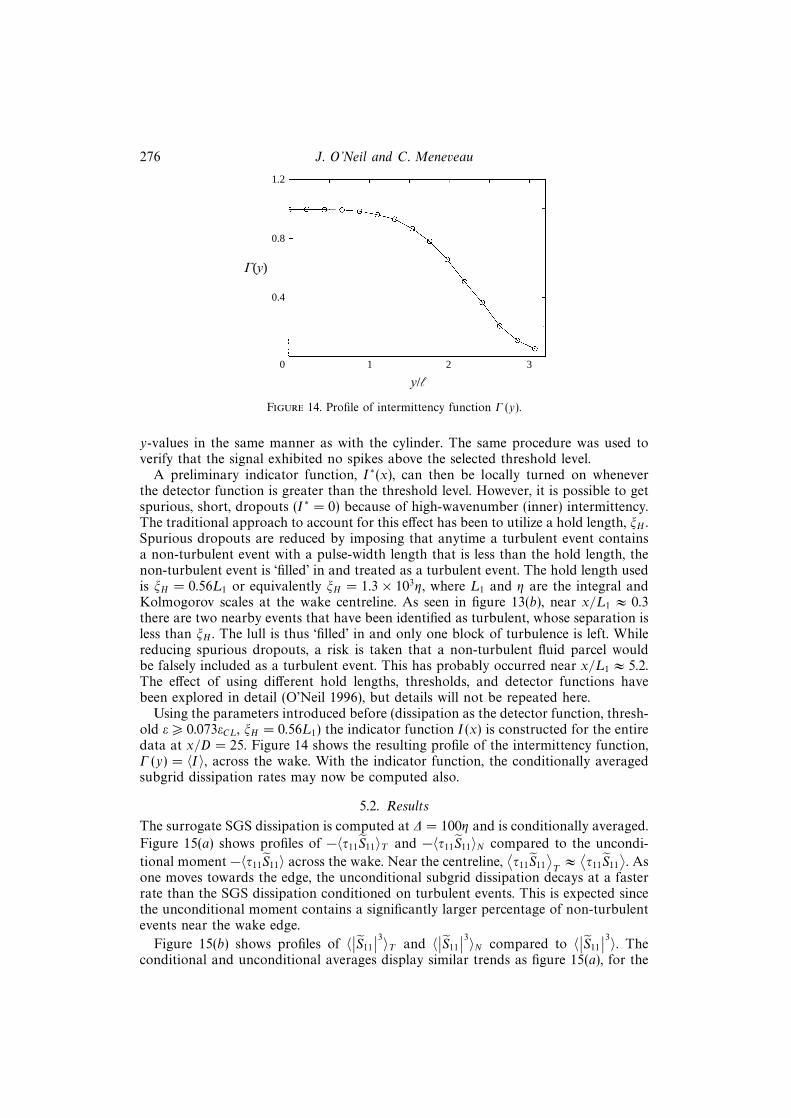
Figure 14. Profile of intermittency function Γ (y).

y-values in the same manner as with the cylinder. The same procedure was used toverify that the signal exhibited no spikes above the selected threshold level.

A preliminary indicator function, I∗(x), can then be locally turned on wheneverthe detector function is greater than the threshold level. However, it is possible to getspurious, short, dropouts (I∗ = 0) because of high-wavenumber (inner) intermittency.The traditional approach to account for this effect has been to utilize a hold length, ξH .Spurious dropouts are reduced by imposing that anytime a turbulent event containsa non-turbulent event with a pulse-width length that is less than the hold length, thenon-turbulent event is ‘filled’ in and treated as a turbulent event. The hold length usedis ξH = 0.56L1 or equivalently ξH = 1.3× 103η, where L1 and η are the integral andKolmogorov scales at the wake centreline. As seen in figure 13(b), near x/L1 ≈ 0.3there are two nearby events that have been identified as turbulent, whose separation isless than ξH . The lull is thus ‘filled’ in and only one block of turbulence is left. Whilereducing spurious dropouts, a risk is taken that a non-turbulent fluid parcel wouldbe falsely included as a turbulent event. This has probably occurred near x/L1 ≈ 5.2.The effect of using different hold lengths, thresholds, and detector functions havebeen explored in detail (O’Neil 1996), but details will not be repeated here.

Using the parameters introduced before (dissipation as the detector function, thresh-old ε > 0.073εCL, ξH = 0.56L1) the indicator function I(x) is constructed for the entiredata at x/D = 25. Figure 14 shows the resulting profile of the intermittency function,Γ (y) = 〈I〉, across the wake. With the indicator function, the conditionally averagedsubgrid dissipation rates may now be computed also.

5.2. Results

The surrogate SGS dissipation is computed at ∆ = 100η and is conditionally averaged.

Figure 15(a) shows profiles of −〈τ11S11〉T and −〈τ11S11〉N compared to the uncondi-

tional moment −〈τ11S11〉 across the wake. Near the centreline,⟨τ11S11

⟩T≈⟨τ11S11

⟩. As

one moves towards the edge, the unconditional subgrid dissipation decays at a fasterrate than the SGS dissipation conditioned on turbulent events. This is expected sincethe unconditional moment contains a significantly larger percentage of non-turbulentevents near the wake edge.

Figure 15(b) shows profiles of 〈∣∣S11

∣∣3〉T and 〈∣∣S11

∣∣3〉N compared to 〈∣∣S11

∣∣3〉. Theconditional and unconditional averages display similar trends as figure 15(a), for the


12

8

4

0

0 1 2 3

(a)

–-s

11S 11

|I(x

). (

m2

s–3)

5

4

3

0

0 1 2 3

(b)

-|S11

|3 )I(

x). (

¬10

6 s–3

)

2

1

–1

y/Fy/F

~

~

Figure 15. (a) The conditional subgrid dissipation for both turbulent and non-turbulent events. (b)The conditional resolved cubed strain rate magnitude for both turbulent and non-turbulent events.Triangles: unconditional moments, squares: non-turbulent averages (I = 0), circles: turbulentaverages (I = 1).

same reasons. However, the turbulent average decays less strongly at the edge thanin figure 15(a). This suggests that the Smagorinsky coefficient in the turbulent regionsagain decays, at the outer portions of the wake.

Most noticeable is the negligible values of the non-turbulent averages comparedto the turbulent ones. The modelled SGS dissipation which was argued to possiblycontain contributions from the outer non-turbulent fluctuating strain is negligiblein the non-turbulent regions of the signal. The implications for the Smagorinskycoefficient are immediate, since one can write

〈τ11S11〉 = Γ 〈τ11S11〉T + (1− Γ ) 〈τ11S11〉N, (33)

and neglecting the non-turbulent part one obtains 〈τ11S11〉 ≈ Γ 〈τ11S11〉T .Given the results of figure 17(b), a similar approximation is warranted for the

Smagorinsky term,⟨∣∣S ∣∣3⟩ ≈ Γ⟨∣∣S ∣∣3⟩

T. Replacing in (32) yields that the Smagorinsky

coefficient valid inside the turbulent region is approximately equal to the unconditionalvalue, i.e. CS |T ≈ CS .

Therefore, conditional averaging based on outer intermittency does not yield amore constant model coefficient across the wake. A number of sensitivity studieswere done (O’Neil 1996) and it was found that this conclusion is quite robust withregard to the various parameters that entered the construction of the indicatorfunction.

6. Coherent structures and phase-averagingIn §4, the relationship between SGS dissipation and the mean velocity field of

the wake was explored. This was followed by an analysis of the effect of outerintermittency on the Smagorinsky coefficient, with little dependency found. Anotherfeature of the flow field which is ubiquitous in turbulent shear flows is the presence oflarge-scale coherent structures (Brown & Roshko 1974; Crow & Champagne 1971).Townsend (1956) used measurements of the velocity autocorrelation function in acylinder wake to infer the presence of large quasi-deterministic eddies on top ofthe turbulent scale range. Cantwell (1981) credits him with being the first to drawa concrete picture of organized large-eddy motion and to realize its importance in


controlling turbulent transport. Probably one of the most pronounced features ofthe cylinder wake is the initial formation of organized alternating two-dimensionalvortices, the Karman vortex street. Cantwell & Coles (1983), Hussain & Hayakawa(1987, hereafter denoted HH) and Matsumura & Antonia (1993) have extensivelystudied such wake structures from the point of view of phase-decomposed Reynoldsaveraging, entrainment and transport.

LES has the advantage that such structures are (typically) resolved in the simulation,and need not be modelled. A question that has not been addressed before in thecontext of the plane turbulent wake is what effect coherent structures have onfeatures of the SGS dynamics such as SGS dissipation of kinetic energy. If there isan effect, one wonders how this is represented by the various models. In this section,we employ conditional averaging with respect to coherent structures in the wake tostudy the conditional SGS dissipation and the model predictions.

6.1. Eduction via phase averaging

Roshko (1954) showed that clearly defined periodicity of the Karman vortex streetseemed to disappear at about x/D = 50. Therefore, like the intermittency studyin §5, attention will remain focused solely on the data at x/D = 25. As can beseen from figure 4, there is no peak evident at any wavenumber (frequency) for thestreamwise velocity component. Spectra of vertical velocity, u2, show a dominantand compact peak at the Strouhal frequency. The peak frequency is fS = 87.9 Hz,giving Strouhal number St = 0.181. For reference, Cantwell & Coles’ (1983) datawere at ReD = 1.4 × 105, x/D = 1–8, and they found St = 0.171. HH sampled atReD = 1.3× 104, x/D = 10, 20 and 40, and found St = 0.21. The Strouhal mode andits neighbouring component on each side contain 20% of the total u2-variance. Theamount of energy density at fS is over ten times greater than in the neighbouringincoherent large-scale turbulence. Spectra at other y/` also displayed a similar peak,but of decreasing magnitude as y/` increases.

The ubiquity of the Strouhal peak at all y/` locations allows us to use phaseaveraging to identify coherent structures. Moreover, the results of HH (who useda vertical array of probes for simultaneous measurements across y) clearly showthat the conditional iso-u2 contours are vertically oriented, that is to say the iso-u2

structures are not inclined. This implies that the phases of the sinusoidal componentof u2 at fS are about the same at all y-locations. This in turn means that one may useindependent measurements at different y-locations by traversing a single probe, andsynchronizing the phases of the band-pass filtered u2 signal during post-processing.This is the approach followed by Matsumura & Antonia (1993).

To minimize problems with spectral resolution of fS , long segment sizes shouldbe used to perform the notch filtering in a narrow band around fS = 87.9 Hz. Onthe other hand, using very long segments has the disadvantage that phase-jitter inthe full signal is not accounted for. As a good compromise between these competingrequirements (see O’Neil 1996 for more details), a segment size of 213 points (a lengthof 0.136 s) is used, containing 11–12 periods of the Strouhal signal. The local phase(Φ = 0) is defined for each segment by the first upward zero crossing of the notch-filtered u2 detector signal. No attempt is made to extrapolate outside the first andlast zero crossing of each 213 segment, since the amount of trimmed data is small.Phase-averaged variables are evaluated by discretizing the phase Φ ∈ (0, 2π) into mbins and conditionally averaging variables for each bin.


30

20

10

0 40 80 120 160 200 0

0.1

0.2

0.310

8

6

4

2

0

(a) (b)

0.2 0.4 0.6 0.8 1.0

U/2pNumber of points (¬103)

–-s

11S 11

|U.

(m2

s–3)

-|S113

|)U. (¬

104

s–3)

r/[–

-s11

S 11.)

]

~

~

~

Figure 16. (a) Convergence history (running averages) of −⟨τ11S11|Φ

⟩(solid line, left-hand scale)

and⟨|S11|3|Φ

⟩(dotted line, right-scale), in dimensional form. Data are at the centreline, at ∆ = 200η.

There were m = 10 bins used for the conditional averaging. (b) Root-mean-square of the last halfof the convergence history, normalized by the actual or modelled SGS dissipation.

6.2. Statistical convergence

The next concern is with statistical convergence of small-scale variables measuredwith the single-wire probe. In earlier sections, all 2× 106 points at each location wereavailable for averaging. Now, only a fraction 1/m of the data is available at eachphase. One possible estimate for the convergence uncertainty is to evaluate ‘runningconditional averages’ using from a few to the total of 2× 106 m−1 points to computethe averages. Figure 16(a) shows running averages of both the real and Smagorinskydissipation at a certain phase (Φ = 0), from data obtained at the centreline, witha filter of ∆/η = 200. The discretization uses m = 10, meaning that 105 points areavailable in each bin. Clearly the Smagorinsky term converges significantly better thanthe real SGS dissipation. It is well known that convergence of turbulence odd-order

moments (such as⟨τ11S11

⟩) is more difficult to achieve than for even-order (or the

absolute values of odd-order) moments. The degree to which such variables attaintheir asymptotic value may be quantified by evaluating the r.m.s. of the runningaverages over the last half of the data, that is, using from 106 m−1 to 2 × 106 m−1

points. Figure 16(b) plots this r.m.s. for the phase-averaged SGS and Smagorinskydissipations. The values are normalized with the respective mean SGS dissipation

averaged over all 2 × 106 points without phase averaging. While⟨∣∣S3

11

∣∣∣∣Φ⟩ doesrelatively well (with σ typically below 3%) at all phases, the actual SGS dissipationhas larger errors (with σ between 5% and 15%). The worst convergence is for thebin at Φ = 0, for which the running averages are shown in (a). The other binsdisplay better convergence histories. Similar results were obtained by using m = 20and m = 30. The main focus of the analysis of phase-averaged distributions will bequalitative, for which the present convergence accuracy is deemed acceptable.

From here on, phase-averaged variables will be denoted by⟨. . .⟩c, and the explicit

reference to phase Φ will be omitted for convenience.

6.3. Construction of pseudo-two-dimensional contours

Data at each y/` are phase discretized into m = 20 bins. The velocities are expressedin a coordinate system convecting with the rollers at a speed Uc, defined as themean velocity at the y/` location at which the peak vorticity is observed (see below).To enhance visual clarity, the data are extended in both the y- and the (pseudo)streamwise direction. Periodicity is employed to plot a total range of phase equal to


4π. Furthermore, the data are extended in the −y-direction by assuming symmetryand phase reversal about the centreline (since measurements were only performedon one side of the wake). Adding an additional bin at Φ = 4π (equal to the valuesat Φ = 0), the total data matrix is then 41 × 29. To reduce jitter in the contours, amoving two-dimensional average is applied to the fields, over the four neighbouringbins (2 in each direction). The data matrix is thus reduced to 40× 28 bins.

6.4. Coherent velocity field

Figure 17 shows results pertaining to the phase-averaged velocity field. The⟨u1

⟩c

and⟨u2

⟩c

components from the x-wires are plotted as velocity vectors. Note that only one-quarter of the figure is measured, the other three quadrants being obtained as outlinedin the preceding section. The

⟨u1

⟩c

component is reduced by Uc = 22.54 m s−1, sincethe frame is moving at Uc in the streamwise direction. The flow is from left to right.There are three roll centres on the top, and two on the bottom. Conversely, there aretwo saddle points above the centreline, and three below it. The agreement betweenthis phase-averaged vector field with the educed fields from HH is good, even thoughsome differences in the eduction method exist and the present Reynolds number ishigher. The vertical extent of the figures corresponds to 6.2`. The horizontal extent is2×Uc/fS = 6.9` (using Taylor’s hypothesis with the roller convection velocity).

The coherent spanwise vorticity is defined as⟨ω3

⟩c≡∂⟨u2

⟩c

∂x−∂⟨u1

⟩c

∂y, (34)

and is evaluated from the phase-averaged velocities. The vorticity is then normalizedby the wake half-velocity-defect height and wake deficit velocity, Us = 3.23 m s−1. Theminimum and maximum scaled vorticity is ±1.36, and is located at the roll centres,yc/` = ±0.88. This gives the location at which Uc =

⟨u1 (yc)

⟩is obtained. Figure

17(a) shows the conditional spanwise vorticity contours. The vectors are superimposedon the vorticity contours as an aid in locating the critical points and structure inthe field. The contours are given at ten discrete evenly spaced levels between theminimum and maximum values. There seems to be good spatial agreement with thecontours from HH. They measured a peak vorticity magnitude of

⟨ω3

⟩c/Sm = 6, where

SmD/U∞ = 0.105 was the maximum mean shear. The maximum mean shear for thisexperiment is SmD/U∞ = 0.0611, so that the maximum strength of the vorticity fieldis⟨ω3

⟩c/Sm = 1.90. This discrepancy is probably due to the differences in eduction

scheme. The vortices of HH are stronger, since unlike the phase-averaging used here,HH only kept about 13% of the data, rejecting the rest as non-coherent events.

Contours of⟨S11

⟩c

=⟨∂u1/∂x

⟩c

are shown in figure 17(b). The coherent strain⟨S12

⟩c

is evaluated according to

⟨S12

⟩c

=1

2

(∂⟨u1

⟩c

∂y+∂⟨u2

⟩c

∂x

). (35)

Contours are shown in figure 17(c), and are substantially stronger than⟨S11

⟩c. Maxima

are located at the saddles, and⟨S12

⟩c

is very weak at the roll centres.

The incoherent Reynolds shear stress −⟨u′1u

′2

⟩c

(where u′i = ui −⟨u1

⟩c) is shown

in figure 17(d). Again, data from the x-wires have been employed. Extrema are atthe saddle points, and contours are slightly inclined along the separatrix. This agreesrather well with the results of HH. If −

⟨u′1u

′2

⟩c

is normalized with U2∞ instead, the


(a) (b)

(c) (d )

–1.35 1.35 –0.150 0.147

–0.56 0.56 –0.15 0.15

Figure 17. Vectors: conditionally averaged velocity field in a frame moving with the rolls, in theintermediate wake of a cylinder at x/D = 25. Velocity magnitude of arrows at corners is 2.24 m s−1.

Contours in (a) correspond to the phase-averaged spanwise vorticity⟨ω3

⟩c/(Us/`), (b) contours

of⟨S11

⟩c/(Us/`), (c) contours of

⟨S12

⟩c/(Us/`), (d) contours of incoherent Reynolds shear stress

−⟨u′1u

′2

⟩c/U2

s .

incoherent Reynolds stress intensity levels become ±0.24, as compared to the HHresults of ±0.5. Also, some discrepancies with the incoherent normal Reynolds stressesof HH were observed. Again, discrepancies are due most probably to the less stringenteduction scheme used here.

These results show that phase averaging applied to the current data set at x/D = 25yields expected behaviour in terms of the coherent fields, and important incoherentvariables such as Reynolds shear stress.


(a) (b)

(c) (d )

–0.05 1.70 –0.035 1.61

0 1.40 0 1.19

Figure 18. Contours of phase-averaged surrogate SGS dissipation − 152〈τ11S11〉c, normalized with

the centreline dissipation εCL. Results are for a Gaussian filter. (a) ∆/η = 300, (b) ∆/η = 200, (c)∆/η = 100, (d) ∆/η = 50. As in figure 17 and in all subsequent figures, vectors correspond tophase-averaged velocity.

6.5. Phase-averaged SGS dissipation

The phase-averaged SGS dissipation is now measured, using the single-wire data. Asbefore, subgrid-scale isotropy is assumed to hold also for the conditionally averagedstatistics, so that we evaluate the surrogate SGS dissipation according to⟨

τij Sij⟩c≈ 15

2

⟨τ11S11

⟩c. (36)

Results are shown in figure 18, normalized with the global viscous dissipation εCL atthe centreline. The different plots are for different filter sizes, from ∆/η = 300 downto 50. The first conclusion that can be drawn from these results is that there is a clear


1.2

0.8

0.4

0101 102 103

D/g

r sS, –

15 2-s

11S 11

./ε C

L˜

Figure 19. Circles: degree of spatial non-uniformity of phase-averaged surrogate dissipationrate along Φ, as a function of filter width. This non-uniformity is quantified by means of theroot-mean-square value at y/` = 0.88. Also shown (squares) is the global mean value of the surro-gate SGS dissipation at y/` = 0.88, showing an approximate plateau near εCL, characteristic of aninertial range.

correlation, or effect, of the coherent structure on the surrogate SGS dissipation field.At any fixed y/` there are marked changes along the phase. While the peaks in overallmean SGS dissipation were located at the centreline, the peaks in phase-averaged dissi-pation are at the height of the roll centres. However, the peaks are concentrated at theroll fronts, not their centres. It is tempting to raise the possibility that this is related tosecondary structures (ribs). The ribs are believed (see HH) to be stretched by the sad-dle and then merge with the spanwise rolls at about the location where the surrogateSGS dissipation peaks are located. It is quite possible that such merging is associatedwith strong transfer of energy from large to small scales (or SGS dissipation).

Such an interpretation must be tempered with a reminder of the strong assumptionsthat underlie the analysis (SGS isotropy and one-dimensional filtering). However, atthe very least we may conclude that there is a strong effect of coherent structure on thesubgrid dynamics. If SGS isotropy holds, then the results imply that there is a strongeffect on the SGS dissipation. If SGS isotropy does not hold, then the results implythat there is a strong effect on the 1-1 component, and on small-scale anisotropy.

Another observation in figure 18 is that the distributions appear to become moreuniform in the horizontal (streamwise) direction as the filter size decreases. Animportant element in the Kolmogorov phenomenology of the turbulence energycascade is that small scales become independent of large scales as the scale ratioincreases. In the present context, if the SGS scales were independent of large-scalephenomena, one would expect uniform distributions of the phase-averaged SGSdissipation in the streamwise direction. In order to quantify the spatial non-uniformity

of SGS dissipation, the root-mean-square of − 152

⟨τ11S11

⟩c

is computed over x (or phaseΦ), at a fixed y-location. Such an r.m.s., σ, can be computed for various filter lengthsaccording to

σ2 =

mm∑i=1

(− 15

2

⟨τ11S11

∣∣Φi⟩c)2

−(

m∑i=1

(−⟨

152τ11S11

∣∣Φi⟩c))2

m (m− 1), (37)

where m = 20 bins. The y-location is y/` = 0.88, where⟨ω3

⟩c

is maximum. The


(a) (b)

(c) (d )

0.02 1.11 0.02 1.17

0.03 1.24 0.03 1.20

Figure 20. Contours of phase-averaged surrogate Smagorinsky dissipation 153/2(0.06∆)2〈|S11|3〉c,normalized with the centreline dissipation εCL. Results are for a Gaussian filter. (a) ∆/η = 300, (b)∆/η = 200, (c) ∆/η = 100, (d) ∆/η = 50.

results are shown in figure 19. The mean value − 152

⟨τ11S11

⟩is superimposed on the

same figure. With an order of magnitude change in ∆ (say between ∆ = 800η and80η), there is only a 30% decrease in the spatial r.m.s. of SGS dissipation, in thephase-averaged contours. This result shows that the approach to independence oflarge and small scales, if it exists, is surprisingly slow. In agreement with the findingsof Piomelli et al. (1996) in channel flow, we conclude that there is a strong correlationbetween coherent flow structures at large scales and SGS dissipation at much smallerscales.


(a) (b)

(c) (d )

–0.12 1.27 –0.05 1.36

–0.03 1.32 –0.01 1.20

Figure 21. Contours of phase-averaged surrogate dissipation of the similarity model, − 152〈L11S11〉c,

normalized with the centreline dissipation εCL. Results are for a Gaussian filter. (a) ∆/η = 300, (b)∆/η = 200, (c) ∆/η = 100, (d) ∆/η = 50.

6.6. Phase-averaged models of SGS dissipation

Next, the properties of SGS models are examined. The energy dissipation producedby the Smagorinsky model, using (23) but phase-averaged, is shown in figure 20 fordifferent filter sizes. A constant Smagorinsky coefficient of CS = 0.06 was used, basedon the globally averaged results of §4.2. Clearly, the distribution is quite differentfrom the distribution of the SGS dissipation in figure 18. The peak values are moreuniformly distributed along the centreline, with some preference towards the rollcentres as opposed to their fronts. Thus, the presence of rollers appears to have amuch weaker effect on fluctuating strain (which enters directly in the Smagorinskymodel) than on the real nonlinear energy transfer.


(a) (b)

(c) (d )

–0.42 2.29 –0.18 2.51

–0.05 2.62 –0.03 2.23

Figure 22. Contours of phase-averaged surrogate dissipation predicted by the dynamic Smagorin-

sky model, 153/2(∆2〈L11M11〉c/〈M11M11〉c) 〈|S11|3〉c, normalized with the centreline dissipation εCL.Results are for a Gaussian filter. (a) ∆/η = 300, (b) ∆/η = 200, (c) ∆/η = 100, (d) ∆/η = 50.

The phase-averaged SGS dissipation using the similarity model is shown in figure21. A value CL = 1.0 is used. As can be seen by comparing these distributions withfigure 18, the similarity model captures the qualitative features of the real distributionmuch better than the Smagorinksy model. The spatial agreement with the actual SGSdissipation is quite good with regions of peak forward scatter agreeing both in termsof location and up to about 20% in intensity. This also agrees with the findings ofPiomelli et al. (1996) who found more realistic conditional flow structures based onthe similarity model than based on the Smagorinsky model.

The dynamic Smagorinsky model is investigated next, again at various filter lengthsbetween ∆ = 50η and 300η. We measure a conditional dynamic coefficient by phase


averaging the numerator and denominator in (26). The predicted conditional SGSdissipation is then obtained according to

− 153/2∆2 〈L11S11〉c〈M11M11〉c

〈|S11|3〉c. (38)

Results are shown in figure 22, and are normalized by εCL. Comparing to the actualSGS dissipation in figure 18 shows a qualitative resemblance. However, when com-paring magnitudes, there are discrepancies: about 50% too much dissipation in thefront of the rolls, and too much backscatter in the outer part of the wake. In §4.4it was found that the dynamic model (evaluated with the present assumptions andone-dimensonal simplifications) gave a 25% overestimate of the global coefficient. Asignificant discrepancy in conditional averages is therefore not too surprising. Never-theless, we can conclude that the qualitative features of the real SGS dissipation arereproduced much better with the dynamic model than with the regular Smagorinskymodel.

6.7. Similarity model with cutoff filter

It is well known that the correlation coefficient between the actual SGS stress andthe similarity model is high when using Gaussian and top-hat filters (well localizedin physical space), but is very low when using a cutoff filter in wave space (seee.g. Liu et al. 1994). In that reference, this effect was attributed to ‘ringing’, namelyspatial oscillations that arise due to Gibbs phenomenon when filtering spatially localstructures with a cutoff filter. While this argument is plausible in explaining the lowcorrelation displayed by the cutoff-filtered similarity model during a priori tests, thequestion remains whether there is any support for the similarity model if a cutofffilter is used, as would be the case in a spectral simulation.

The phase-averaged dissipation predicted by the similarity model using cutoff filtersis examined, and is compared with the real dissipation where the stress and strainrate are also evaluated using the cutoff filter. The comparison is performed at filterlengths of ∆ = 200η and 50η. Figure 23 displays the results, again normalized by εCL.At larger filter sizes the results are quite comparable to those of the Gaussian filter,although the SGS magnitudes are slightly larger at the peaks. The same is true at∆ = 50η, except for the fact that some additional oscillations (jitter) can be discernedin the contours. Also, there are more discrepancies between the modelled and real SGSdissipation than for the case of Gaussian filter shown in figure 18. Nevertheless, thequalitative features of the conditional SGS dissipation are still reproduced. The modelpredicts local peaks of forward SGS dissipation at the roll fronts. From the pointof view of phase-averaged SGS dissipation, this result suggests that the similaritymodelling approach has merit (at least over the plain Smagorinsky model) even whendealing with spectral cutoff filters.

6.8. Phase-decomposed SGS dissipation

In the previous section, the dissipation of the entire resolved kinetic energy fieldwas studied with phase averaging. In this section, the resolved field is first phasedecomposed to exclude the coherent field from the interaction between resolved andunresolved scales.

The phase-averaged SGS dissipation may be decomposed as follows:

−⟨τij Sij

⟩c

= −(⟨τij⟩c

⟨Sij⟩c

+⟨τ′ij S

′ij

⟩c

), (39)


(a) (b)

(c) (d )

–0.02 1.72 –0.08 2.11

1.26 0 1.730

Figure 23. Contours of phase-averaged surrogate SGS dissipation using the sharp cutoff instead

of Gaussian filter. (a) Real dissipation − 152〈τ11S11〉c at ∆/η = 200. (b) Dissipation predicted by

similarity model at ∆/η = 200 with spectral cutoff filter. (c) Real dissipation at ∆/η = 50. (d)Similarity model with cutoff filter at ∆/η = 50.

where τ′ij = τij − 〈τij〉c and S ′ij = Sij −⟨Sij⟩c. The first term in (39) may be interpreted

as the energy that is transferred from (or to) the coherent field towards (or from) thesubgrid scales, while the second represents energy transferred between all remainingresolved scales and the SGS range.

To see more clearly that −⟨τij′S ′ij⟩c

is indeed the energy dissipation from resolved,but incoherent, motion to unresolved motion, an incoherent resolved kinetic energyequation is derived, following Reynolds & Hussain (1972). Denoting the incoherentpart of the velocity as u′i, one may define the incoherent, but resolved, kinetic energy


–0.23 0.250 –0.02 1.40

Figure 24. Contours of phase-decomposed surrogate SGS dissipation. (a) Contribution from coher-

ent part, − 152

⟨τ11

⟩c

⟨S11

⟩c, corresponding to energy flux between the coherent field and the subgrid

scales. (b) Energy flux between incoherent (but resolved) field and subgrid scales, − 152

⟨τ11′S ′11

⟩c.

Results are for Gaussian filter, at ∆/η = 200.

according to12e2 = 1

2u′iu′i. (40)

One starts with the resolved momentum equation for the total filtered velocity ui.Then, all of the primitive variables including the SGS stress are decomposed into acoherent and incoherent part. A second equation is formed by phase averaging andthe difference is taken to obtain an equation for the incoherent resolved velocity:

∂u′i∂t

+⟨uj⟩c

∂u′i∂xj

= − ∂

∂xj

(p′

ρδij −

⟨u′iu′j

⟩c

+ u′iu′j +⟨u′i⟩cu′j + τij

′ − 2νS ′ij

). (41)

Multiplying by u′i, phase averaging, neglecting the viscous dissipation, and not writingthe transport term in detail yields

∂

∂t

⟨12e2⟩c

+⟨uj⟩c

∂

∂xj

⟨12e2⟩c

= −⟨u′iu′j

⟩c

⟨Sij⟩c

+⟨τij′S ′ij⟩c− ∂

∂xj

⟨...⟩c. (42)

The term −⟨u′iu′j

⟩c

⟨Sij⟩c

is the production of resolved incoherent kinetic energy due tocoherent strain (or dissipation of coherent energy due to resolved incoherent motion).

The term⟨τij′S ′ij⟩c

is indeed the sink (if negative) of resolved, but incoherent, kineticenergy due to the SGS stress.

Next, phase-averaged distributions of − 152

⟨τ11

⟩c

⟨S11

⟩c

and − 152

⟨τ11′S ′11

⟩c

are evalu-ated and shown in figure 24. The filter size was ∆ = 200η, using a Gaussian filter. Itis interesting to note that the levels of the coherent part reach only 16% of the peaktotal dissipation (in figure 18), which while not negligible, is not a dominant effect.

The incoherent SGS dissipation − 152

⟨τ′11S

′11

⟩c

is shown in figure 24(b). Comparedto figure 18, one can see that there is less streamwise modulation by the coherentstructures, especially near the outer edges of the wake where the contour lines aremore horizontal. Nevertheless, near the centreline, the contours still display significant


modulation. The peak still occurs near the roll fronts, but closer to their centre thanthe peaks of full SGS dissipation.

We conclude that there are significant effects of the coherent structure on the SGSdissipation, even when only considering the incoherent portion of this variable.

7. Summary and conclusionsThe primary motivation of this work is to supplement existing numerical a priori

and a posteriori studies of the SGS stress and models with a priori experimental resultsat high Reynolds numbers, in a fairly complex flow field with outer intermittency andregions of coherent structure.

The first part of the study involved globally averaged quantities across the wakeof a cylinder, at four downstream locations. Owing to the need to maximize theturbulence Reynolds number, a fairly large cylinder was chosen leading some featuresof the downstream development of the wake (e.g. r.m.s. velocities) to exceed those ofa canonical free wake.

Based on the measurements, comparisons were made between the actual and mod-elled mean SGS dissipation. Also, the coefficients of the Smagorinsky and similaritymodels, as well as those obtained from the dynamic Smagorinsky model were mea-sured. The surrogate dissipation rate profiles from x/D = 25 to 100 agreed out to thewake half-width, `, when scaled with the centreline total dissipation rate. For y > `,the profiles for lower x/D decayed more slowly. When corrected for the effects of one-dimensional filtering, the measured Smagorinsky coefficient fell inside the expectedrange of 0.1 to 0.12. The viability of the Smagorinsky model was confirmed by show-ing that the constancy of CS was relatively insensitive to variations of the Reynoldsnumber, filter length, and downstream location. A weak cross-stream decrease of CSwas observed for filter scales above ∼ 0.01L1, meaning that the constant-coefficientSmagorinsky model slightly overpredicts SGS dissipation in the outer wake, unless fil-ter scales are about two or more orders of magnitude smaller than the integral scale.This trend is reminiscent of the well-known overprediction of the −u′v′ Reynoldsstress using the mixing-length model in the plane wake. However, conditional av-eraging based on outer intermittency to eliminate possible effects of non-turbulentpatches did not significantly affect this trend. This leads to the conclusion that theweak decrease in CS is not due to outer intermittency but to an inherent difference inthe structure of turbulence, or to anisotropy effects which we could not capture withthe instrumentation, the surrogate dissipation, and limitations of one-dimensionalfiltering.

The similarity model was insensitive to changes in downstream distance, Reynoldsnumber, and filter length, as long as both ∆ and 2∆ remained well inside the inertialrange. As expected, the correlation for the similarity model was considerably higherthan the Smagorinsky model. The dynamic Smagorinsky coefficient was found to be25% higher than the traditional Smagorinsky coefficient, but agreed with its basictrends of a slight decline in the outer part of the wake.

Following the analysis of globally averaged variables, the interaction of coherentstructure and the dynamics of the subgrid motion were studied. The presence oflarge-scale coherent structures was shown to strongly affect the distribution of themeasured surrogate for SGS energy dissipation. This was the case even after phasedecomposing the SGS stress and strain rates, to extract the coherent part of the field.The surrogate SGS dissipation structure was found to become more evanescent withdecreasing filter size, though much of the structure remained even at the small-scale


end of the inertial range, ∆ = 20η. This trend suggests that to reach independencebetween large and small scales requires very large scale separations. It is importantto recall again that the observed changes in surrogate dissipation due to coherentstructures may not only reflect the actual distribution of SGS dissipation, but couldalso reflect varying deviations from the assumed SGS isotropy. At any rate, our resultsclearly show that the coherent structures have a direct effect on SGS dynamics,either in terms of true SGS dissipation or SGS anisotropy (or a combination ofboth).

The Smagorinsky model was unable to reproduce the observed distribution ofsurrogate SGS dissipation with respect to the coherent structures, while the similaritymodel captured the main features as long as the filters were inside the inertial range.The dynamic Smagorinsky model, with the coefficient obtained from phase averaging,did reproduce qualitative features of the (surrogate) SGS dissipation. The similaritymodel with spectral cutoff filtering showed essentially zero correlation with the realstress field, but did display the main characteristics of the structure of surrogate SGSdissipation.

An important as yet unresolved question is what happens further downstream (i.e.at x/D > 50) when the organized Karman vortex street disappears. It is believed thatthere still are ‘coherent structures’ but that they are no longer nicely periodic, i.e. theyare not discernible from phase averaging. How much of present results carry overto the relationship between such non-periodic large-scale structures and the subgridscales is not known, and clearly deserves further study.

In summary, present results provide detailed evidence that SGS modelling basedon ‘learning’ from resolved scales (such as in the dynamic or similarity models)should lead to more realistic predictions than the constant-coefficient eddy-viscositymodel, when turbulence is spatially complex and when coherent structures affect theSGS dynamics directly. At the level of phase-averaged dissipation, both the dynamicSmagorinsky and the similarity models appeared to work well, so that any linearcombination of the two should also provide a good model to reproduce phase-averaged dissipation. In recent years, such mixed models have shown promise in LES(e.g. Zang et al. 1993; Wu & Squires 1995; Vreman et al. 1994). The mixed model isalso advantageous to model the response of SGS turbulence to rapid distortion (Liuet al. 1997).

We thank Professors O. Knio and N. Jones for useful comments and discussions.This work was funded by the National Science Foundation (grant CTS-9408344) andthe Office of Naval Research (grant N00014-92-J-1109). Data analysis and manage-ment were done mostly on an in-house PowerChallenge L supported by NSF (grantCTS-9506077). Some initial analysis was done at the Pittsburgh SupercomputingCenter.

REFERENCES

Adrian, R. J. 1991 Particle-imaging techniques for experimental fluid mechanics. Ann. Rev. FluidMech. 23, 261–304.

Antonia, R. & Atkinson J. 1974 Use of a pseudo-turbulent signal to calibrate an intermittencymeasuring circuit. J. Fluid Mech. 64, 679–699.

Bardina, J., Ferziger, J. & Reynolds, W. C. 1980 Improved subgrid scale models for large eddysimulation. AIAA Paper 80-1357.

Brown, G. & Roshko, A. 1974 On density effects and large structure in turbulent mixing layers. J.Fluid Mech. 64, 775–815.


Cantwell, B. 1981 Organized motion in turbulent flow. Ann. Rev. Fluid Mech. 13, 457–515.

Cantwell, B. & Coles, C. 1983 An experimental study of entrainment and transport in theturbulent near wake of a circular cylinder. J. Fluid Mech. 136, 321–374.

Chen, C. & Blackwelder, R. 1978 Large scale motion in a boundary layer: a study usingtemperature contamination. J. Fluid Mech. 89, 1–32.

Clark, R. G., Ferziger, J. H. & Reynolds, W. C. 1979 Evaluation of subgrid models using anaccurately simulated turbulent flow. J. Fluid Mech. 91, 1–16.

Comte-Bellot, G. & Corrsin, S. 1966 The use of a contraction to improve the isotropy of gridgenerated turbulence. J. Fluid Mech. 25, 657–682.

Cook, A. W. 1997 Determination of the constant coefficient in scale similarity models of turbulence.Phys. Fluids 9, 1485–1487.

Corrsin, S. 1943 Tech. Rep. W-94. NACA Wartime Report.

Corrsin, S. & Kistler, A. 1955 Tech. Rep. 1244. NACA Report.

Crow, C. & Champagne, F. 1971 Orderly structure in jet trubulence. J. Fluid Mech. 48, 547–591.

Deardorff, J. W. 1970 A numerical study of three-dimensional turbulent channel flow at largeReynolds numbers. J. Fluid Mech. 41, 453–480.

Domaradski, J. A., Liu, W. & Brachet, M. E. 1993 An analysis of subgrid-scale interactions innumerically simulated isotropic turbulence. Phys. Fluids A 5, 1747–1759.

Germano, M., Piomelli, U., Moin, P. & Cabot, W. H. 1991 A dynamic subgrid-scale eddy viscositymodel. Phys. Fluids A 3, 1760–1765.

Ghosal, G., Lund, T., Moin, P. & Akselvoll, K. 1995 A dynamic localization model for large-eddysimulation of turbulent flows. J. Fluid Mech. 286, 229–255.

Hartel, C., Kleiser, L., Unger, F. & Friedrich, R. 1994 Subgrid-scale energy transfer in thenear-wall region of turbulent flows. Phys. Fluids 6, 3130–3143.

Hedley, T. & Keffer, J. 1974 Turbulent/non-turbulent decisions in an intermittent flow. J. FluidMech. 64, 625–644.

Hussain, F. & Hayakawa, M. 1987 Eduction of large-scale organized structures in a turbulent planewake. J. Fluid Mech. 180, 193–229 (referred to herein as HH).

Kollman, K. 1982 Intermittent turbulent flow. In Frontiers in Fluid Mechanics (ed. S. Davis & J.Lumley), pp. 88–112. Springer.

Kovasznay, L., Kibens, V. & Blackwelder, R. 1970 Large-scale motion in the intermittent regionof a turbulent boundary layer. J. Fluid Mech. 41, 283–325.

Kraichnan, R. H. 1976 Eddy viscosity in two and three dimensions. J. Atmos. Sci. 33, 1521–1536.

Leonard, A. 1974 Energy cascade in large-eddy simulations of turbulent fluid flows. Adv. Geophys.18, 237–248.

Lesieur, M. & Metais, O. New trends in large-eddy simulations of turbulence. Ann. Rev. FluidMech. 28, 45–82.

Leslie, D. C. & Quarini, G. L. 1979 The application of turbulence theory to the formulation ofsubgrid modelling procedures. J. Fluid Mech. 91, 65–91.

Lilly, D. K. 1967 The representation of small-scale turbulence in numerical simulation experiments.In Proc. IBM Sci. Comput. Symp., pp. 195–209.

Liu, S., Katz, J. & Meneveau, C. 1997 Evolution and modelling of subgrid scales during rapidstraining of turbulence (submitted).

Liu, S., Meneveau, C. & Katz, J. 1994 On the properties of similarity subgrid-scale models asdeduced from measurements in a turbulent jet. J. Fluid Mech. 275, 83–119.

Liu, S., Meneveau, C. & Katz, J. 1995 Experimental study of similarity subgrid-scale models ofturbulence in the far-field of a jet. Appl. Sci. Res. 54, 177–188.

Matsumura, M. & Antonia, R. A. 1993 Momentum and heat transport in the turbulent intermediatewake of a circular cylinder. J. Fluid Mech. 250, 651–668.

Meneveau, C. 1994 Statistics of turbulence subgrid-scale stresses: Necessary conditions and exper-imental tests. Phys. Fluids 6, 815–833.

Meneveau, C., Lund, T. & Cabot, W. 1996 A Lagrangian dynamic subgrid-scale model of turbu-lence. J. Fluid Mech. 319, 353–386.

Monin, A. & Yaglom, A. 1971 Statistical Fluid Mechanics. MIT Press.

Muck, K. C. 1980 Comparison of various schemes for the generation of the turbulent intermittencyfunction. Imperial College Aero Rep. 80-03.


Murlis, J. & Bradshaw, P. 1974 On the measurement of intermittency in turbulent flow. ImperialCollege Aero. Rep. 74-04.

Murray, J., Piomelli, U. & Wallace, J. 1996 Spatial and temporal filtering of experimiental datafor a priori studies of subgrid-scale stresses. Phys. Fluids 8, 1978–1980.

O’Neil, J. 1996 Subgrid-scale stresses and their modelling in the turbulent plane wake. PhD thesis,The Johns Hopkins University.

Oster, D. & Wygnanski, I. 1982 The forced mixing layer between parallel streams. J. Fluid Mech.123, 91–130.

Piomelli, U., Cabot, W., Moin, P. & Lee, S. 1991 Subgrid-scale backscatter in turbulent andtransitional flows. Phys. Fluids A 3, 1766.

Piomelli, U., Moin, P. & Ferziger, J. H. 1988 Model consistency in large eddy simulation ofturbulent channel flows. Phys. Fluids 31, 1884.

Piomelli, U., Yu, Y. & Adrian, R. 1996 Subgrid-scale energy transfer and near-wall turbulencestructure. Phys. Fluids 8, 215–224.

Press, W. H., Teukolsky, S. A., Vetterling, W. T. & Flannery, B. P. Numerical Recipes, 2nd edn.Cambridge University Press.

Reynolds, W. C. & Hussain, F. 1972 The mechanics of an organized wave in turbulent shear flow.Part 3. Theoretical models and comparisons with experiments. J. Fluid Mech. 54, 263–288.

Rogallo, R. & Moin, P. 1984 Numerical simulation of turbulent flows. Ann. Rev. Fluid. Mech. 16,99.

Roshko, A. 1954 On the development of turbulent wakes from vortex streets. Tech. Rep. TN 1191.NACA.

Saddoughi, S. G. & Veeravalli, S. V. 1994 Local isotropy in turbulent boundary layers at highReynolds number. J. Fluid Mech. 268, 333–372.

Scotti, A., Meneveau, C. & Lilly, D. K. 1993 Generalized smagorinsky model for anisotropicgrids. Phys. Fluids A 5, 2306.

Smagorinsky, J. 1963 General circulation experiments with the primitive equations. i. the basicexperiment. Mon. Weath. Rev. 91, 99.

Tennekes, H. & Lumley, J. L. 1972 A First Course in Turbulence. MIT Press.

Townsend, A. 1956 The Structure of Turbulent Shear Flow. Cambridge University Press.

Vreman,B., Geurts, B. & Kuerten, H. 1994 On the formulation of the dynamic mixed subgrid-scalemodel. Phys. Fluids A 6, 4057–4059.

Wu, X. & Squires, K. 1995 Large eddy simulation of a canonical three-dimensional boundary layer.In Proc. Tenth Symp. on Turbulent Shear Flows, Penn State (ed. F. Durst, B. E. Launder, F. W.Schmidt & J. W. Whitelaw).

Zang, Y., Street, R. L. & Koseff, J. 1993 A dynamic mixed subgrid scale model and its applicationto rubulent recirculating flows. Phys. Fluids A 5, 3186.

Subgrid-scale stresses and their modelling in a turbulent ...

Documents

Transcript of Subgrid-scale stresses and their modelling in a turbulent ...