STUDY QUESTIONS - APPLIED NUMERICAL METHODS …fabianc/nummet1.pdf · STUDY QUESTIONS - APPLIED...

STUDY QUESTIONS - APPLIED NUMERICAL METHODS PART

1

1

2 STUDY QUESTIONS - APPLIED NUMERICAL METHODS PART 1

Contents

Question 1-8, By Mengxi Wu 3Question 9-17, Solutions by Mengxi Wu, Written by Patrik Rufelt 6Question 18-26, By Henrik Sjöström 9Question 27-35 By Elin Hynning 12Question 36-44 By Lars-Lowe Sjösund 19Question 45-51, By Olof Bergvall 24Question 52-54, By Gustav Sædén Ståhl 28Question 55-60, By Alexander Eriksson 30

STUDY QUESTIONS - APPLIED NUMERICAL METHODS PART 1 3

Question 1-8, By Mengxi Wu

1. Given a system of ODE's y = Ay, where A is an nn-matrix. Give asucient condition that the analytical solution is bounded for all t > 0.Will there be bounded solutions when the matrix A = ...? (p.21). Ananalytical solution which is stable as t→∞ must be bounded. The stability of theODE system is stable if all the eigenvalues ,λi, of A has a real parts that satisesRe(λi) < 0. In other words the eigenvalues are situated in the left half the complexplane and is asymptotically stable, hence the solution will always be bounded.

However if Re(λi) = 0, then the system is stable if every λi is unique. If thereexistsRe(λi) = 0 and there are λi which are the same, then you have to investigatethe specic case for stability.

2. For a nonlinear system of ODE's y = f(y), what is meant by thecritical points of the system? Give a sucient condition that a criticalpoint is stable. Are the critical point of the following system stable?(p.23). A point y is a critical point of the system if it satises f(y) = 0. Thispoint is also referred to as the stationary or steady- state solutions.

If we perturbed y to y + δy(t) in a neighborhood of y, then the critical pointis asymptotically stable if all the perturbed solution converges to y. If there is anyperturbed solution which diverges from y then the critical point is unstable.

3. Given a nonlinear system of ODE's y = f(y). Assume that theright hand side consists of dierentiable functions. Describe a New-ton's method for computing the critical points of the system. For thefollowing system, choose an initial vector and make one iteration withNewton's method. (p.181). Newton's method is based on Taylor expansion off(y) at a point y(i), where y(i) is an estimate of a critical point. The function f(y)is assumed to be twice dierentiable. We have:

f(y) ≈ f(y(i)) + J(y(i))(y − y(i)) +O

Where J(y(i)) is the Jacobian of f(y), i.e ∂f∂y .

Since we are searching for critical points we seek f(y) = 0, we can set the lefthand side to 0 and obtain:

f(y(i)) + J(y(i))(y − y(i)) = 0

This gives us:

y(i+1) = y(i) − f(y(i))

J(y(i))

With a start guess u(0), we iterate until we nd the critical point.

4. What does it mean that an n × n matrix A is diagonalizable? Is thefollowing matrix A diagonalizable? A is diagonalizable means that we canwrite it as a product of its eigenvectors and values in the following manner:

A = SΛS−1

where S contains the eigenvectors s1, s2, . . . , sn and Λ is a diagonal matrix contain-ing λ1, λ2, . . . , λn.A is diagonalizable when it has n linearly independent eigenvectors.


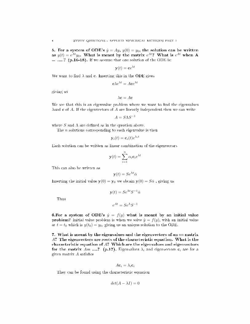
5. For a system of ODE's y = Ay, y(0) = y0, the solution can be writtenas y(t) = eAty0. What is meant by the matrix eAt? What is eAt when A= .....? (p.16-18). If we assume that one solution of the ODE is:

y(t) = ceλt

We want to nd λ and c. Inserting this in the ODE gives

cλeλt = Aceλt

giving us

λc = Ac

We see that this is an eigenvalue problem where we want to nd the eigenvaluesλand c of A. If the eigenvectors of A are linearly independent then we can write

A = SΛS−1

where S and Λ are dened as in the question above.The n solutions corresponding to each eigenvalue is then

yi(t) = ci(t)eλit

Each solution can be written as linear combination of the eigenvectors

y(t) =

n∑i=1

αicieλt

This can also be written as

y(t) = SeΛtα

Inserting the initial value y(0) = y0 we obtain y(0) = Sα , giving us

y(t) = SeΛtS−1α

Thus

eAt = SeΛS−1

6.For a system of ODE's y = f(y) what is meant by an initial valueproblem? Initial value problem is when we solve y = f(y), with an initial valueat t = t0 which is y(t0) = y0, giving us an unique solution to the ODE.

7. What is meant by the eigenvalues and the eigenvectors of an nnmatrixA? The eigenvectors are roots of the characteristic equation. What is thecharacteristic equation of A? Which are the eigenvalues and eigenvectorsfor the matrix A= ....? (p.17). Eigenvalues λi and eigenvectors ci are for agiven matrix A satises

Aci = λici

They can be found using the characteristic equation

det(A− λI) = 0


8.Given a dierence equation yn+1 = a1yn + a2yn−1 + ....+ ak+1yn−k, wherea1, a2, ..., ak+1 are real. Formulate a sucient condition that the sequenceyn is bounded for all n. Is the solution bounded when n > 0 for the follow-ing dierence equation? ... (p.185. The characteristic equation correspondingto the homogenous part of the dierence equation is then

a1µk + a2µ

k−1 + . . .+ ak+1 = 0

If we denote the roots of the characteristic equation as µ1, µ2, µ3, . . . , µk. Asn → ∞ then sequence yn is bounded if |µi| ≤ 1 if all the roots are unique. If theroots are not unique then |µi| < 1.


Question 9-17, Solutions by Mengxi Wu, Written by Patrik Rufelt

9. Given a dierence equation on the form ∇yn + 12∇

2yn = 0. Is thesolution yn bounded for all n > 0?

Answer: ( Pages: 185-186 )We let: ∇yn = un − un−1 and ∇2yn = un−2 − 2un−1 − un inserted in the equationgives:

un − un−1 +1

2[un−2 − 2un−1 − un] = 0

3

2un − 2un−1 +

1

2un−2 = 0

un −4

3un−1 +

1

3un−2 = 0

with the char. eq. µ2− 43µ+ 1

3 = 0 which has the following roots: 23 ±

√13 which is

unstable since:∣∣∣ 23 ±√ 1

3

∣∣∣ > 1.

10. Formulate the following 3rd order ODE as a system of three rstorder ODE's ......

Answer: ( Pages: 13-14 )If you are unsure on how to rewrite a nth order ODE as a system of n rst orderODE's, read pages 13-14.

11. Give the recursion formula when the Euler backward method withtime step h is used on e.g. the ODE-problem y′ = y3 + t, y(0) = 1. Ineach time step tn + 1 a nonlinear. equation must be solved. Formulatethat equation on the form F (yn + 1) = 0 and the iteration formula whenNewton's method is applied to this equation.

Answer: ( Euler backward: 42, Newtons method: )Euler Backward: uk = uk−1 + hf(uk, tK), tk = tk−1 + h

y′k = −y3k + tk =⇒ yk − yk−1

h= −y3

k + tk =⇒

=⇒ y3k −

yk − yk−1

h− tk = 0 = F (yk) = 0

yi+1 = yi −[(yik)3 − yik−y

ik−1

h − tk]

3(yik)2 − 1/h.

12. What is meant by an explicit method for solving an initial valueproblem

y = f(y), y(0) = y0

Give at least two examples (with their formulas) of explicit methodsoften used to solve such a problem.


Answer: ( Pages: 42, 55 )An Explicit method only uses the data we aldready know to calculate the next step,examples: Euler forward: uk = uk−1 + hf(uk−1, tk−1), tk = tk−1 + hRunge-kutta: uk = uk−1 + h

6 (k1 + 2k2 + 2k3 + k4), tk = tk−1 + hWhere:

k1 = f(uk−1, tk−1)

k2 = f(uk−1 + hk1

2, tk−1 +

h

2)

k3 = f(uk−1 + hk2

2, tk−1 +

h

2)

k4 = f(uk−1 + hk3, tk−1 + h)

.

13. What is meant by an implicit method for solving an initial valueproblem

y = f(y), y(0) = y0

Give at least two examples of implicit methods (with their formulas)often used to solve such a problem.

Answer: ( Pages: 42, 54 )An Implcit method uses data from the current step, examples:Euler backwards: uk = uk−1 + hf(uk, tk), tk = tk−1 + hTrapezodial method: uk = uk−1 + h

2 (f(uk, tk) + f(uk−1, tk−1)), tk = tk−1 + h.

14. What is meant by the order of accuracy for a method used to solvean initial value problem

y = f(y), y(0) = y0

What is the order of the Euler forward method and the classical Runge-Kutta method?

Answer: ( Pages 44, 55)Error relation e ≈ cp, where p is the order of accuracy.Accuracy of Euler forward: order 1Accuracy of classical Runge-Kutta (RK4): order 4.

15. What is meant by automatic stepsize control for a method used tosolve an initial value problem y = f(y), y(0) = y0?

Answer:(1) Accept step k if δ ≤ tol(2) Reject step k if δ > tol, restart from tk−1 with new stepsize hnew = h

2 , returnto (1).

16.Why is the midpoint method not suited for ODE-systems where theeigenvalues of the jacobian are real and negative? Are there any ODE-systems for which the method could be suitable?


Answer:(Leap frog) midpoint method is used to solve: y′(t) = f(t, y(t)), y(t0) = y0 O(h2)uk = uk−2 + 2hf(tk−1, uk1)tk = tk−1 + h, k = 2, 3, ..., NApply u = f = λu, thus we get the deerence eq.⇒ uk = uk−2 + 2hλuk−1 − uk−2 = 0Char eq. of dierence equation isµ2 − 2λhµ− 1 = 0,(µ− µ1)(µ− µ2) = 0, µ1µ2 = 1, (µ1 + µ2) = 2hλWrite one root in polar form: µ1 = reiφ, for stable solution r=1, (|µ1| < 1, forstability) µ1 + µ2 = 2hλ → eiφ − e−iφ = 2hλ → 2i sin(φ) = 2hλ hλ = i sin(φ)Only imaginary values in stability region.

17. Explain the dierence between local error and global error for theexplicit Euler method.

Answer:Global error: ek = u(tk)− uk = O(h)This is also known as truncation error which can be regarded as the eect of all thelocal errors up to the point tk (Note that this is seldomly the sum of all the localerorrs)Summation: How much it diers from the "real" value up to step tk.

Local error: l(tk, h) = u(tk)−u(tk−1)h − f(tk−1, u(tk−1))

Can be regarded as the residual when the exact solution is inserted into the expliciteuler. Local error is basically the error in one single point.In conclusion: Global error: error up to a certain point.Local error: error in one point.


Question 18-26, By Henrik Sjöström

(2) 18. An ODE-problem, initial value and boundary value problem, can besolved by a discretization method or an ansatz method. Give a brief description ofwhat is meant by these two method classes.

Discretization: Approximating the derivative by calculating the dierance be-tween nearby points resulting in a set of equations that can be used to nd thesolution in the discretised set.

Ansatz: Approximating the solution with a best t from a set of ansatz equa-tions, often exponential functions.

(4) 19. When an initial value problem y = f(y), y(0) = y0 is solved with adiscretization method, what is meant by the stability area in the complex hq-planefor the method? Give a sketch of the stability area for the method .........

The area in the complex plane where the solution is numericly stable for theproduct λh.

To get the stability area of a method replace y′ with an appropriate approxi-mation of the derivative and f(y) with the eigenvalue λi of the jacobian J(f(y)).By rewriting the equation on the form yk+1 = a(λ)yk the solution converges ifRe(λ) ≤ 0 and |a(λ)| < 1 then calculate for what values of the product λh thesecond condition is fulllled. That is the stability area.

(2) 20. What is meant by a sti system of ODE's y = f(y)?

A system where the eigenvalues λi of the jacobian J(f(y)) are orders of magni-tude dierent from each other and ∀i it holds that Re(λi) ≤ 0.

(2) 21. For a linear system of ODE's y = Ay, where the eigenvalues of A areλ1, λ2, ..., λn , when is the system stable? Assume that all eigenvalues are real andnegative, when is the system sti?

The system is stable when Re(λi) < 0 ∀i and is considered sti when dierentλ are of very dierent sizes. Usually diering with factors of 102 or larger.

(2) 22. Describe some discretization methods that are suitable for sti initialvalue ODE problems.

Euler implicituk−uk−1

h = f(tk, uk) from this equation one solves for uk, usually this needs tobe done in every step making the method somewhat inecient.

Trapezoidal methodA symmetric combination of eulers implicit and explicit methods.2uk−uk−1

h = f(tk, uk) + f(tk−1, uk−1) this method is not recommended for verysti problems.


Both euler implicit and the trapezoidal method neccesates to solve for uk in ev-ery step.

(2) 23. Which is the computational problem when a sti initial value ODE-system is solved with an explicit method?

A very large spread for λ requires a very high accuracy i.e small step h and solv-ing for many points since the part of the equation corresponding to a small λ willmost likely be interesting to study for a longer period of time. Thus the problembecomes very expensive to solve.

(3) 24. Given e.g. the following ODE-system y = −100y+z, y(0) = 1, z = −0.1z,z(0) = 1. For which values of the stepsize h is the Euler forward method stable?Same question for the Euler backward method.

calculate the eigenvalues of the system u = Au by the equation det(A− Iλ) = 0.In this case: λ1 = −100 and λ2 = −0.1

Euler explicit makes the approximation of the derivative according touk+1−uk

h = Auk this gives the equation uk+1 = uk + hAuk replacing A by its

eigenvalue λ gives uk+1 = (1 + hλ)uk = (1 + hλ)ku0 this converges if |1 + hλ| < 1in this particular case we have that for 0 < h < 1

50

Euler implicit makes the approximation of the derivative according touk+1−uk

h = Auk+1 this gives the equation uk+1 = uk + hAuk+1 replacing A by

its eigenvalue λ gives uk+1(1 − hλ) = uk and further uk+1 = (1 − hλ)−ku0 thisconverges if |1− hλ|−1 < 1 in this particular case we have that for h > 0

(4) 25. Given the vibration equation mx + cx + kx = 0, x(0) = 0, x(0) = v0.Use scaling of x and t to formulate this ODE on dimensionless form. Determinescaling factors so that the scaled equation contains as few parameters as possible.

Set x = aξ and t = bτ . Insert into ∂2x∂t2 = a

b2∂2ξ∂τ2 and ∂x

∂t = ab∂ξ∂τ .

Rewriting the equation and inserting the above into x+ cm x+ k

mx→ aξ+ acb2

bm ξ+akb2

m ξ = 0, removing a and setting b = mc

ξ + ξ +mk

c2ξ

with x(0) = v0 = aξ(0)b selecting a = v0b we get

ξ(0) = 1

(2) 26. Describe the nite dierence method used to solve a boundary valueproblem y′′ + a(x)y′ + b(x)y = c(x), y(0) = a, y′(1) + y(1) = b

Replacing the derivatives with the central dierance approximations,y′k = yk+1−yk−1

2h

y′′k = yk+1−2yk+yk−1

h2


yk+1 − 2yk + yk−1

h2+ a(x)

yk+1 − yk−1

2h+ b(x)yk =

(1

h2+a(x)

2h)yk+1 + (

−2

h2+ b(x))yk + (

1

h2− 1

2h)yk−1 = 0

(1

h2+a(x)

2h)yk+1 + (

−2

h2+ b(x))yk + (

1

h2− 1

2h)yk−1 = c(x)

This gives N equations with N+2 unknown. y(0) = a gives us the value of the

unknown y0, and y′N + yN = yN+1−yN−1

2h + yN = b gives us one more equation, thenwe have suciently much information to solve the system and can set up a systemof equations and solve for all values of yk ∀k. This results in a tridiagonal systemof equations that can be set up and solved nummerically.


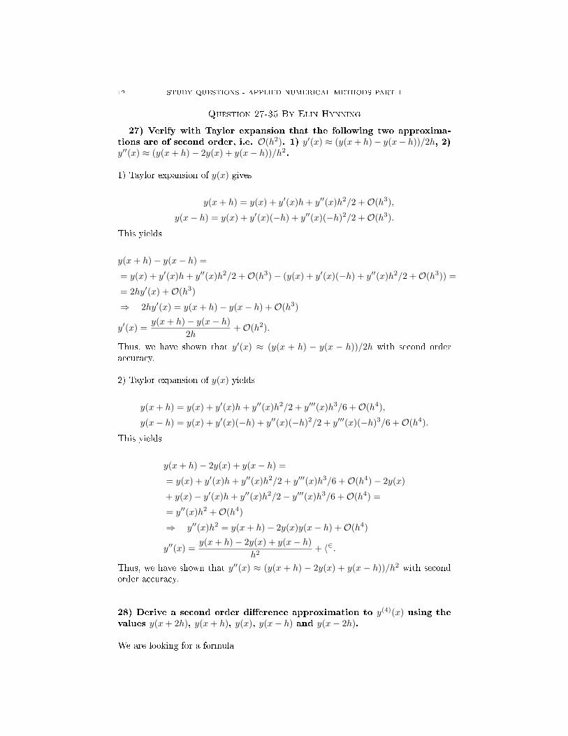
Question 27-35 By Elin Hynning

27) Verify with Taylor expansion that the following two approxima-tions are of second order, i.e. O(h2). 1) y′(x) ≈ (y(x+ h)− y(x− h))/2h, 2)y′′(x) ≈ (y(x+ h)− 2y(x) + y(x− h))/h2.

1) Taylor expansion of y(x) gives

y(x+ h) = y(x) + y′(x)h+ y′′(x)h2/2 +O(h3),

y(x− h) = y(x) + y′(x)(−h) + y′′(x)(−h)2/2 +O(h3).

This yields

y(x+ h)− y(x− h) =

= y(x) + y′(x)h+ y′′(x)h2/2 +O(h3)− (y(x) + y′(x)(−h) + y′′(x)h2/2 +O(h3)) =

= 2hy′(x) +O(h3)

⇒ 2hy′(x) = y(x+ h)− y(x− h) +O(h3)

y′(x) =y(x+ h)− y(x− h)

2h+O(h2).

Thus, we have shown that y′(x) ≈ (y(x + h) − y(x − h))/2h with second orderaccuracy.

2) Taylor expansion of y(x) yields

y(x+ h) = y(x) + y′(x)h+ y′′(x)h2/2 + y′′′(x)h3/6 +O(h4),

y(x− h) = y(x) + y′(x)(−h) + y′′(x)(−h)2/2 + y′′′(x)(−h)3/6 +O(h4).

This yields

y(x+ h)− 2y(x) + y(x− h) =

= y(x) + y′(x)h+ y′′(x)h2/2 + y′′′(x)h3/6 +O(h4)− 2y(x)

+ y(x)− y′(x)h+ y′′(x)h2/2− y′′′(x)h3/6 +O(h4) =

= y′′(x)h2 +O(h4)

⇒ y′′(x)h2 = y(x+ h)− 2y(x)y(x− h) +O(h4)

y′′(x) =y(x+ h)− 2y(x) + y(x− h)

h2+ 〈∈.

Thus, we have shown that y′′(x) ≈ (y(x + h) − 2y(x) + y(x − h))/h2 with secondorder accuracy.

28) Derive a second order dierence approximation to y(4)(x) using thevalues y(x+ 2h), y(x+ h), y(x), y(x− h) and y(x− 2h).

We are looking for a formula


y(4)(x) = ay(x+ 2h) + by(x+ h) + cy(x) + dy(x− h) + ey(x− 2h) +O(h2)

Taylor expansion yields

y(4) = a(y + y′2h+ y′′2h2 + y′′′4h3/3 + y(4)2h4/3)+

+b(y + y′h+ y′′h2/2 + y′′′h3/6 + y(4)h4/24)+

+cy + d(y − y′h+ y′′h2/2− y′′′h3/6 + y(4)h4/24)+

+e(y − y′2h+ y′′2h2 − y′′′4h3/3 + y(4)2h4/3) +O(h5)

Thus, we obtain the following system of equations:

a+ b+ c+ d+ e = 0

2ah+ bh− dh− e2h = 0

a2h2 + bh2/2 + dh2/2 + e2h2 = 0

a4h3/3 + bh3/6− dh3/6− e4h3/3 = 0

a2h4/3 + bh4/24 + dh4/24 + e2h4/3 = 1

We may write this on matrix form:1 1 1 1 12 1 0 −1 −24 1 0 1 48 1 0 −1 −816 1 0 1 16

abcde

=24

h4

00001

Solving this system yields

a =1

h4, b =

−4

h4, c =

6

h4, d =

−4

h4, e =

1

h4.

Now we need to determine the order of the error. We look at the next term inthe Taylor expansion, namely

ay(5)16h5/15 + by(5)h5/120− dy(5)h5/120− ey(5)16h5/15.


Since b = d and a = e it holds that this term is zero. Thus, we look at theterm following the previous in the Taylor expansion:

ay6(2h)6/6! + by6(h)6/6! + dy6(h)6/6! + ey6(2h)6/6!

This term will obviously not be zero, and thus our error will be of the order h6

h4 = h2.Thus, we may write

y(4)(x) =y(x+ 2h)− 4y(x+ h) + 6y(x)− 4y(x− h) + y(x− 2h)

h4+O(h2)

29) Derive a second order dierence approximation to y′(x) using thevalues y(x), y(x− h) and y(x− 2h).

We are looking for a formula on the form

y′(x) = ay(x) + by(x− h) + cy(x− 2h) +O(h2).

Taylor expansion yields

y′(x) = ay(x) + b(y(x)− y′(x)h+ y′′(x)h2/2) + c(y(x)− 2y′(x)h+ 2y′′(x)h2) +O(h3).

This yields the following equations:

a+ b+ c = 0

−bh− 2ch = 1

bh2/2 + 2ch2 = 0

We may write this on matrix form: 1 1 10 −1 −20 1 4

abc

=1

h

010

Solving this system yields

a =3

2h, b = − 4

2h, c =

1

2h.


Since the coecients are of order h−1 and we know that the rst possible non-zero term we have not taken into account is of order h3, we may deduce that wehave an error term of order h2. Thus, we may write the rst derivative of y(x) inthe following way:

y′(x) =3y(x)− 4(x− h) + y(x− 2h)

2h+O(h2)

30) Given a second order ODE y′′ = f(x, y, y′). Assume a Dirichlet bound-ary value is given in the left interval point y(0) = 1. Present two otherways in which a boundary condition can be given in the right bound-ary point. For second order BVP's there are three kinds of boundary conditions.Apart from the above mentioned Dirichlet boundary conditions, which consist ofspecifying the solution at the boundary, there are Neumann boundary conditionsand Robin boundary conditions or Mixed boundary conditions. The Neumann BC'sconsist of specifying the derivative at the boundary. The Robin BC's species acombination of y′(x) and y(x) at the boundary.

31) When a boundary value problem y′′ = p(x)y′ + q(x)y + r(x), y(0) =1, y(1) = 0 is solved with discretisation based on the approximationsy′′(xn) ≈ (yn+1 − 2yn + yn1)/h2 and y′(xn) ≈ (yn+1 − yn1)/2h we obtain alinear system Ay = b of equations to be solved. Set up this system.Which special structure does the matrix A have? In order to set up thesystem we start by substituting the discretised derivatives into the equation. Thisyields

yn+1 − 2yn + yn1

h2≈ pn

yn+1 − yn1

2h+ qnyn + rn,

where pn = p(xn) and so on. Rearranging the above expression yields

(1

h2− pn

2h

)yn+1 −

(2

h2+ qn

)yn +

(1

h2+pn2h

)yn−1 = rn.

We may thus express the equation as the following system of equations:

Ay = b,

where

A =

c2 c3 0 0 · · · 0c1 c2 c3 0 · · · 0

0. . .

. . .. . .

... 00 · · · 0 c1 c2 c30 · · · 0 0 c1 c2

,

where c1 = 1h2 + pn

2h , c2 = − 2h2 − qn and c3 = 1

h2 − pn2h . Moreover, we have


b =

r1

r2

...rN−1

,

y1

y2

...yN−1

,

where y0 = y(0) and yN = y(1). Since the boundary conditions state that y0 =yN = 0, we do not need to include these points in our y-vector. If the boundaryconditions were not zero, they would have been included in the b-vector.

The matrix A is said to be tridiagonal, since all nonzero elements lie on the threecentermost diagonals of A.

32) What is meant by a tridiagonal n×n matrix A? The number of opsneeded to solve a corresponding linear system of equations Ax = b can beexpressed as O(np). What is the value of p? The number of bytes neededin the memory of a computer to store such a system can be expressed asO(nq). What is the value of q? A tridiagonal n×n matrix A is an n×n-matrixwhere all the nonzero elements are situated at the three centermost diagonals ofthe matrix.

If the tridiagonal matrix algorithm (TDMA) is used, the number of ops neededto solve the linear system Ax = b is O(n), i.e. p = 1.

(Source: http://en.wikipedia.org/wiki/Tridiagonal_matrix_algorithm)One may store the elements of a tridiagonal matrix in an n×3-matrix, thus only

requiring the storage of 3n elements. The number of bytes needed to store A in thememory of a computer may therefore be expressed as O(n), i.e. q = 1.

33) What is meant by a banded n × n matrix A? Describe some way ofstoring such a matrix in a sparse way. Same question for a prole matrix.A banded n × n-matrix A is a matrix where all non-zero elements are situated atcentral diagonals of the matrix. If a banded matrix has p diagonals containingnon-zero elements, these diagonals may be stored as vectors in an n× p-matrix.

Prole storage of a matrix is a storage type applicable for symmetric positivedenite (SPD) matrices. Since the matrix is symmetric, we only need to storethe diagonal and the entries below the diagonal. The prole of the matrix is theborder for which all elements to the left of the border are zero-elements. A prolematrix can be stored in the following way: All nonzero elements of A are stored ina vector a. The elements are stored row by row, starting from the rst element inthe prole. Together with a, a pointer vector p is also stored. The elements of phold the indices in a for the diagonal elements of A. (See page 197 in Edsberg'sbook for an example).

34) What input and output data are suitable for a Matlab functionsolving a tridiagonal system of linear equations Ax = b if the goal is tosave number of ops and computer memory? If we want to save computermemory and number of ops, it is wise to give the input matrix A as a sparsematrix.

(I have no idea of what he is looking for with this question.)


35) The boundary value problem −y′′ = f(x), y(0) = y(1) = 0 can besolved with an ansatz method based on Galerkin's method. Formulatethe Galerkin method for this problem. The Galerkin method starts with anansatz on the form

y(x) ≈ y(x) =

N∑j=1

cjϕj(x),

where ϕj(x) are given basis functions and cj are coecients to be determined sothat y(x) is a good approximation. We assume that the basis functions satisfythe boundary conditions, i.e.

ϕj(0) = ϕj(1) = 0 ∀j.

If we insert the ansatz into the BVP we get the following residual function

r(x) = y′′(x) + f(x) 6= 0.

Preferably, we want r(x) to be small. Galerkin's method deals with this in thefollowing way: We demand r(x) to be orthogonal to the basis functions. This maybe expressed as ∫ 1

0

r(x)ϕj(x)dx = 0 ∀j

Inserting the expression for r(x) yields

∫ 1

0

N∑j=1

cjd2ϕjdx2

+ f(x)

ϕidx = 0 ∀j, i

N∑j=1

cj

∫ 1

0

d2ϕjdx2

ϕidx+

∫ 1

0

f(x)ϕidx = 0 ∀j, i.

We perform partial integration on the integral in the rst term:

∫ 1

0

d2ϕjdx2

ϕidx =

[dϕjdx

ϕi

]1

0

−∫ 1

0

dϕjdx

dϕidx

dx = −∫ 1

0

dϕjdx

dϕidx

dx.

The last equality follows from the fact that ϕj(0) = ϕj(1) = 0.Insert the expression for the integral into the expression for r(x) yields


N∑j=1

cj

∫ 1

0

dϕjdx

dϕidx

dx =

∫ 1

0

f(x)ϕidx ∀i, j.

This is a linear system of equations Ac = b, where

ai,j =

∫ 1

0

dϕjdx

dϕidx

dx, bi =

∫ 1

0

f(x)ϕidx.


Question 36-44 By Lars-Lowe Sjösund

36. Classify the following PDEs with respect to linearity (linear or nonlinear), or-der (rst, second), type (elliptic, parabolic, hyperbolic):a) ut = uxx + u,b) uxx + 2uyy = 0,c) ut = (a(u)ux)x,d) ut + uux = 0,e) uy = uxx+ x

Givet diekv. Auxx + 2Buxy + Cuyy +Dux + Euy + F = 0Denna är elliptisk om

Z =

(A BB C

)är positivt denit. Om det(Z)=0 är den parabolisk och om det(Z)<0 hyperbolisk.Ordningen bestäms av högsta förekommande ordning av derivata.

a) det(Z)=0 ⇒ Parabolisk, den är linjär och av ordning 2.b) Z har egenvärdena 1 och 2, alltså är Z positivt denit och ekv. är elliptisk.Ordningen är 2 och ekv. är linjär.c) Ickelinjär, ordning 2, parabolisk (kursboken ekv (5.8))d) Ickelinjär, ordning 1, hyperbolisk (kursboken ekv (5.10))e) Ickelinjär, ordning 1, Oklart...

37. Formulate the ODE-system u = Au + b when the Method of Lines is appliedto the PDE-problem ut = uxx + u, t > 0, 0x1, u(0, t) = 0, u(1, t) = 1, u(x, 0) = xuxx is approximated by the central dierence formula.

Notation: u(xi, tj) = ui,j

Given PDE:

ut = uxx + u

ut(xi) ≈ui−1,j − 2ui,j + ui+1,j

h2x

+ ui,j =ui−1,j + (−2 + h2

x)ui,j + ui+1,j

h2x

Sätt a = 1, b = −2 + h2x.

Vi får systemet

˙u = Au+ b

, där


A =1

h2ξ

b a 0 · · · · · · 0a b a 0 · · · 00 a b a 0 · · ·...

. . .. . .

. . ....

...0 0 · · · a b a0 · · · 0 a b

och

b =1

h2x

0

01

.

A är en N*N-matris där N är antalet inre punkter. Vi får b då u(1, t) = 1.Initialvärdena diskretiseras enligt ui(0) = xi.

38. Formulate the ODE-system u = Au + b when the Method of Lines is appliedto the PDE-problem ut + ux = 0, t > 0, 0x1, u(0, t) = 0, u(x, 0) = x ux is to beapproximated by the backward Euler dierence formula.

Givet PDE ut + ux = 0, vi får diskretiseringen

ut ≈ −ui,j − ui−1,j

hx

Sätt a = 1hx

och b = − 1hx. Vi får systemet

˙u = Au+ b

, där

A =1

hx

b 0 0 · · · · · · 0a b 0 0 · · · 0a b a 0 0 · · ·...

. . .. . .

. . ....

...0 0 · · · a b a0 · · · 0 a b

och

b = 0


.A r en (N+1)*(N+1)-matris, där N är antalet inre punkter (till skillnad från

uppgift 37 har vi inget randvärde vid x=1 och tvingas beräkna värdet själva, däravN+1). Initialvärdet diskretiseras pss som i uppgift 37.

39. What is meant by an upwind scheme for solving ut + aux = 0, a > 0? (2)Upwind scheme för ut+aux = 0, a > 0 innerbär Forward time, backward space

⇒ ui,j+1 − ui,jht

+ aui,j − ui−1,j

hx= 0.

FTBS är av första ordningens noggrannhet i t- och x-led och har stabilitetskriterium0 < a ht

hx1

40. Derive a dierence approximation and the corresponding stencil to e.g. theLaplace operator

∂2u

∂x2+∂2u

∂2y+∂u

∂x+∂u

∂y

Vi drar till med approxmation av andra ordningen (att den verkligen är av andraordn. visas i uppgift 41):

uxx+uyy+ux+uy ≈ui−1,j − 2ui,j + ui+1,j

h2x

+ui,j−1 − 2ui,j + ui,j+1

h2y

+ui+1,j − ui−1,j

2hx+ui,j+1 − ui,j−1

2hy=

= ui−1,j [1

h2x

− 1

2hy]+ui,j [−

2

h2x

− 2

h2y

]+ui+1,j [1

h2x

+1

2hx]+ui,j−1[

1

h2y

− 1

2hy]+ui,j+1[

1

h2y

+1

2hy] =

= c1 ∗ ui−1,j + c2 ∗ ui,j + c3 ∗ ui+1,j + c4 ∗ ui,j−1 + c5ui,j+1

Molekyl:

41. What is the order of accuracy in t and x when the Method of Lines with centraldierences in the x-variable and the implicit Euler method is applied to e.g. theheat equation ut = uxx?

Vi använder centraldierens i x-led, denna är av andra ordningen, ty:

u(x+ h) = u(x) + u′(x)h+ u′′(x)h2

2+ u′′′(x)

h3

6+O(h4)


u(x− h) = u(x)− u′(x)h+ u′′(x)h2

2− u′′′(x)

h3

6+O(h4)

⇒ u(x+ h) + u(x− h) = 2u(x) + u′′(x)h2 +O(h4)

⇒ u(x+ h)− 2u(x) + u(x− h)

h2= u′′(x) +O(h2)

Medelst samma metod eller enligt s.42 i kursboken är impl. Euler av ordning 1.

42. Give a second order accurate approximation dierence formula of (d(x)ux)x.

(d(x)ux)x = dxux + duxx

dx =d(x+ h)− d(x− h)

2h+O(h2)⇒ di+1 − di−1

2h+O(h2)

ux =u(x+ h)− u(x− h)

2h+O(h2)⇒ ui+1 − ui−1

2h+O(h2)

uxx =ui+1 − 2ui + ui−1

h2+O(h2)

(d(x)ux)x =di+1 − di−1

2h

ui+1 − ui−1

2h+O(h2) + di

ui+1 − 2ui + ui−1

h2+O(h2))

43. Describe the Crank-Nicolson method for solving the heat equation.Från wikipedia, först en beskrivning av metoden i allmänhet.

The CrankNicolson method is based on central dierence in space, and thetrapezoidal rule in time, giving second-order convergence in time. For example, inone dimension, if the partial dierential equation is

∂u

∂t= F (u, x, t,

∂u

∂x,∂2u

∂x2)

then, letting u(i∆x, n∆t) = uni , the equation for CrankNicolson method is theaverage of that forward Euler method at n and that backward Euler method atn+ 1 (note, however, that the method itself is not simply the average of those twomethods, as the equation has an implicit dependence on the solution):

un+1i − uni

∆t= Fni

(u, x, t,

∂u

∂x,∂2u

∂x2

)(forward Euler)

un+1i − uni

∆t= Fn+1

i

(u, x, t,

∂u

∂x,∂2u

∂x2

)(backward Euler)

un+1i − uni

∆t=

1

2

(Fn+1i

(u, x, t,

∂u

∂x,∂2u

∂x2

)+ Fni

(u, x, t,

∂u

∂x,∂2u

∂x2

))(Crank-Nicolson)

The function F must be discretized spatially with a central dierence.Note that this is an implicit method: to get the "next" value of u in time, a

system of algebraic equations must be solved. If the partial dierential equation isnonlinear, the discretization will also be nonlinear so that advancing in time will in-volve the solution of a system of nonlinear algebraic equations, though linearizationsare possible. In many problems, especially linear diusion, the algebraic problemis tridiagonal and may be eciently solved with the tridiagonal matrix algorithm,which gives a fast O(n) direct solution as opposed to the usual O(n3) for a full


matrix.

Applicerat på värmeledningsekvationen

The CrankNicolson method is often applied to diusion problems. As an ex-ample, for linear diusion,

∂u

∂t= a

∂2u

∂x2

whose CrankNicolson discretization is then:

un+1i − uni

∆t=

a

2(∆x)2

((un+1i+1 − 2un+1

i + un+1i−1 ) + (uni+1 − 2uni + uni−1)

)or, letting r = a∆t

2(∆x)2 :

−run+1i+1 + (1 + 2r)un+1

i − run+1i−1 = runi+1 + (1− 2r)uni + runi−1$

,which is a tridiagonal problem, so that un+1

i , may be eciently solved by usingthe tridiagonal matrix algorithm in favor of a much more costly matrix inversion.

2D

When extending into two dimensions on a uniform Cartesian grid, the derivationis similar and the results may lead to a system of band-diagonal equations ratherthan tridiagonal ones. The two-dimensional heat equation

∂u

∂t= a

(∂2u

∂x2+∂2u

∂y2

)can be solved with the CrankNicolson discretization of

un+1i,j = uni,j +

1

2

a∆t

(∆x)2

[(un+1i+1,j + un+1

i−1,j + un+1i,j+1 + un+1

i,j−1 − 4un+1i,j )

+ (uni+1,j + uni−1,j + uni,j+1 + uni,j−1 − 4uni,j)]

44. Formulate the Galerkin method for the elliptic problem

uxx + uyy = f(x, y), (x, y) ∈ Ω

u(x, y) = 0, (x, y) ∈ Ω

Galerkins metod står bra beskriven i boken. Grundläggande princip på s.86-88.Från sid.140 behandlas problem 44, man får dock byta ut f(x,y) mot -f(x,y), dåboken behandlar ∆u = −f och problem 44 ∆u = f .


Question 45-51, By Olof Bergvall

Q.45. Formulate the Galerkin method for the parabolic problem,

ut = uxx, u(x, 0) = f(x), u(0, t) = u(1, t) = 0.

Solution: (See Edsberg p.123-124.) Below follows a derivation of the Galerkinformulation as well as the actual formulation. The actual Galerkin formulation isgiven on the next page.

We express u(x, t) as a time-dependent linear combination of basis functions ϕi

u(x, t) =

∞∑i=1

ci(t)ϕi(x),

where each ϕi satisfy the BC ϕi(0) = ϕi(1) = 0. We now approcimate u by therst N terms of the above sum (for some suitable N),

u(x, t) ≈ u(x, t) =

N∑i=1

ci(t)ϕi(x).

Inserting u into the PDE gives,

ut ≈ uxx, ⇐⇒N∑i=1

dci(t)

dtϕi(x) ≈

N∑i=1

ci(t)d2ϕi(x)

dx2.

Since u is an approximation we will not have exact equality in general. Hence, it isinteresting to consider the residual function r(x, t) = ut − uxx. We have,

r(x, t) =

N∑i=1

dci(t)

dtϕi(x)−

N∑i=1

ci(t)d2ϕi(x)

dx2.

We now impose the condition that r(x, t)⊥ϕi(x) for i = 1, . . . , N and all t, i.e.∫ 1

0

r(x, t)ϕi(x)dx = 0, for i = 1, . . . , N, and all t.

This gives,

(*)

N∑i=1

dci(t)

dt

∫ 1

0

ϕi(x)ϕj(x)dx−N∑i=1

ci(t)

∫ 1

0

d2ϕi(x)

dx2ϕj(x)dx = 0.

Consider the second integral in the expression above. By partial integration weobtain,

−∫ 1

o

d2ϕi(x)

dx2ϕj(x)dx = −

[dϕi(x)

dxϕj(x)

]1

0

+

∫ 1

0

dϕi(x)

dx

dϕj(x)

dxdx =

=

∫ 1

0

dϕi(x)

dx

dϕj(x)

dxdx,

since ϕj(0) = ϕj(1) = 0. Inserting this into (*) gives a system of ODE's called theGalerkin formulation of the problem,

Mdc

dt+Ac = 0,


where,

Mij =

∫ 1

0

ϕi(x)ϕj(x)dx, and Aij =

∫ 1

0

dϕi(x)

dx

dϕj(x)

dxdx.

The IC's are obatined from,

u(x, 0) =

N∑i=1

ci(0)ϕi(x) = f(x).

(Here Edsberg does something weird since his f is named u0 and f is a function ofthe PDE). By multiplying with ϕj(x) and integrating over [0, 1] we obtain

(**) Mc(0) = f,

where,

fj =

∫ 1

0

f(x)ϕj(x)dx.

By solving (**) we obtain the intial values of ci(t).

Q.46. In an ansatz method for a 1D problem the solution u(x) is approximatedby the linear expression uh(x) =

∑αiϕi(x), where the basis functions ϕi(x) can

be chosen dierently. Give a description of the roof-functions, i.e. the piecewiselinear basis functions in x.

Solution: (See Edsberg p.88-89.) Let h be the stepsize in a equidistant discretisa-tion of the x-interval in the problem. Let xi denote the ith point of the discretisa-tion. The roof-functions, ρi(x),are then dened as,

ρi(x) =

0, if x ≤ xi−1,1h (x− (i− 1)h), if xi−1 ≤ x ≤ xi,− 1h (x− (i+ 1)h), if xi ≤ x ≤ xi+1,

0, if xi+1 ≤ x.

Intuitively, the roof-functions can be thought of as triangles with corners in (xi−1, 0),(xi, 1) and (xi+1, 0).

Q.47. In an ansatz method for a 2D problem the solution u(x, y) is approximatedby the linear expression uh(x, y) =

∑αiϕi(x, y), where the basis functions ϕi(x, y)

can be chosen dierently. Give a description of the pyramid-functions, i.e. thepiecewise linear basis functions in x, y.

Solution: (See Edsberg p.142-143.) Suppose that we have discretised the regionof our 2D problem and thus obtained points (x1, y1), . . . , (xn, ym). The pyramid-function ρij(x, y) is dened as the function which is zero everywhere except on thequadrangle with cornes (xi+1, yj), (xi, yj+1), (xi−1, yj), (xi, yj−1). On this quadran-gle ρij describes a pyramid, i.e. if we see the quadrangle as a subset of R3 thenρij connects the sides of the quadrangle to the point (xi, yj , 1) with lled triangles.To describe the pyramid explictly as a function of x and y seems to become rathermessy (we have to subdivide the quadrangle into four triangles and dene ρij asfour ane (linear) functions over the respective triangles in a way similar toQ.46.).


Q.48. When solving PDE-problems in 2D and 3D with dierence or ansatz meth-ods we are lead to solving large linear systems of equations Ax = b. What is meantby a direct method and an iterative method for solving Ax = b? Give examples byname of some direct methods and some iterative methods.

Solution: (See Edsberg Appedix A.5.) A direct method is one where the systemis solved directly, i.e. in each step an unknown is solved for and a solution isobtained terms of the unknows not already solved for.

An iterative method is a method where one starts at some initial guess andsuccesively computes better approximations to the solution.

The standard direct method is Gaussian elimination. Often one makes thismethod more ecent by applying e.g. LU-factorisation or Cholesky-factorisation.Examples of iterative methods are Jacobi's method and Gauss-Seidel's method.

Q.49. What is meant by dissipation and dispersion when a conservation law issolved numerically?

Solution: (See Edsberg p.147.) Suppose that we solve a conservation law nu-merically. It may occur that the property that should be conserved is not, dueto numerical eects. This phenomenon is called dissipation (or, more accurately,numerical dissipation).

It may also occur that the phase relations are distorted from what they shouldbe and that the wave speed is variable even though it should be constant, becauseof numerical properties of our algorithm. This phenomenon is called (numerical)dispersion.

Q.50. What is meant by ll-in when solving a sparse linear system of equationsAx = b with a direct method?

Solution: (See Edsberg p.137.) When solve the system directly, for instance usingGaussian elimination, some of the zeros of the matrix A may become nozero in theprocess. (In the case of Gaussian elimination this occurs when we add or subtracta nonzero element to a zero element). We then say that there is a ll-in in A, sincesome of the zero elements are lled with nonzero elements.

Q.51. What is meant by the Cholesky-factorization of a symmetric positive denitematrix A? Can the following matrix A be Cholesky factorized?

Solution: (See Edsberg p.194.) The Cholesky-factorisation of a symmetric andpositive denite matrix A is a factorisation of A as a product of a lower triangularmatrix L and its transpose i.e. A = LLT . (We can generalise to A being a complexhermitian (equal to its conjugate transpose) matrix but then we must take theconjugate transpose of L and we then have the decompostion A = LL∗).

We have not been given any matrix so the second question is somewhat hard toanswer, but what one has to check is if A is symmetric (hermitian in the complexcase) and positive denite. One checks if A is symmetric simply by inspection. Tocheck if A is positive denite one may compute the eigenvalues of A. If they are allpositive, then A is positive denite. If A is very large (so that the charcteristic equa-tion gets a uncomfortably high degree) we may instead compute the determinantsof the north-westmost (upper left corner) 1×1, 2×2, 3×3, . . . , n×n-submatrices ofthe n×n matrix A (i.e. the leading principal minors of A). If they are all positive,


then A is positive. This is tedious, but it does not involved solution of polynomialequations of high degree.


Question 52-54, By Gustav Sædén Ståhl

Q.52 If Ax = b is rewritten on the form x = Hx+c and the iteration xk+1 = Hxk+cis dened, what is the condition on H for convergence of the iterations to thesolution of Ax = b? Also formulate a condition on H for fast convergence.

Solution. The idea is to look at a split of the matrix A as, say, A = M − Nfor some matrices M and N . Then we get Ax = b ⇔ Mx = Nx + b. We want tond the x for when this is fullled, and that we can do by rst guessing a solutionx0 and then iterating by the formula Mxk+1 = Nxk + b and keep doing this until‖xk+1 − xk‖ is as small as we want. Of course, if we choose M to be invertible wecan rewrite this iterative process as

xk+1 = M−1Nxk +M−1b = Hxk + c.

Let G = M−1N , then, in order to study the convergence, we consider the eigenval-ues of G and let

ρ(G) = maxi|λi(G)|.

The following result is is not really derived in the book but I suppose that it comesfrom the fact that rk = Aek where rk is the residual and ek is the error and we getconvergence if ek → 0 as k →∞. The result, however, is that if ρ(G) < 1 we haveconvergence. Also, the convergence is faster the smaller ρ(G) is. A little trivia:ρ(G) is called the spectral radius of G.

Q.53 What is meant by the steepest descent method for solving Ax = b, where Ais symmetric and positive denite?

Solution. When we consider the previous question for a symmetric, positivedenite matrix A (SPD) we get a special case (which might have been seen in thebasic course of optimization, for those of you who have taken that course, but I'mnot 100% sure). For this problem, to nd the solution x to the system of equationsAx = b is equivalent to minimizing the function F (x) = 1

2x>Ax−x>b with respect

to x. Next, in order to minimize this we use a so called search function, which isdened by

xk+1 = xk + αkdk

where dk is the search direction and αk is the stepsize in that direction. Apparantlyit follows immeadiatly that the optimal value of αk is

αk =r>k dk

d>k Adk.

Now we can dene what the steepest descent method is! It is the method wherewe let dk = rk and use starting guess x0 = 0. This simply means that we go in thedirection of the residual when we search for our mimimizer.

Q.54 Describe the preconditioning when used with the steepest descent method.Assume that the matrix A is symmetric and positive denite.

Solution. The convergence of the steepest descent method is related to thecondition number

κ(A) =maxiλi(A)

miniλi(A).

If κ is large, the convergence is slow and if it is small, the convergence is fast. If thecondition number is large we can reduce it with preconditioning. We introduce a


quadratic matrix E and y = Ex. With this substitution we get that a transformedfunction

F (y) = F (x) =1

2y>Ay− y>b

where A = E−>AE−1 and b = E−>b. We now want to choose E such thatκ(A) << κ(A). If E = I we do not change anything so that wouldn't work. If E =

L>, where L is the Cholesky factor of A, then we would have perfect condition, butthe Cholesky factor is to expensive to calculate. Therefore, something in between

of I and L> is a good choice. Then we dene C = E>E as the preconditioningmatrix. A common choice for C is C = diag(A) (which is the same as choosingE = diag(

√a11,√a22, ...,

√ann)).


Question 55-60, By Alexander Eriksson

Q55. For a hyperbolic PDE in x and t the solution u(x, t) is constant along certaincurves in the x, t-plane. What are these curves called? Give the analytic expressionfor these curves belonging to ut + 2ux = 0.

A55. They are called characteristics (page 150), and are the lines resultingfrom the ODE dx

dt = a(u(x(t), t)) (in the x, t plane). First, a general case to explainwhere a(u) comes from, with the equation being:

(0.1)∂u

∂x+

∂

∂xf(u) = 0

f(u) is called the ux function. If f(u) is twice dierentiable, we can insteadrewrite it to

(0.2)∂u

∂x+ a(u)

∂u

∂x= 0

Along a characteristic, the solution is constant, shown simply by du(x(t),t)dt = 0

(nal step; Look at the original equation)

(0.3)du(x(t), t)

dt=∂u

∂t+dx(t)

dt

∂u

∂x=∂u

∂x+ a(u(x(t), t))

∂u

∂x= 0

Constant solution uC along a characteristic gives, with the denition of a char-acteristic:

(0.4)dx

dt= a(uC) = aC −→ x(t) = aCt+ C

In our case, a = 2 which is a constant, and the analytic expression becomessimply x(t) = 2t+ C.

(Characteristic curves can be used to generate entire solutions; If you know theboundary value and the initial condition and you have a collection of curves thatdescribe how that initial solution propagates, you can solve the entire system)

Q56. Given the system of PDEs

(0.5) ut +

(0 12 0

)ux = 0

Is the system hyperbolic? Which are the characteristics?

A56. An hyperbolic system of PDE's occurs if the matrix A(u) is diagonizable and

has real eigenvalues (for this matrix, λ1 =√

2, λ2 = −√

2), where A(u) is takenfrom the setup:

(0.6)∂u

∂x+

∂

∂xf(u) =

∂u

∂x+A(u)

∂u

∂x= 0

A(u) is the jacobian of f(u). Yes, the system is hyperbolic, as the eigenval-ues of A are real and distinct.

The characteristic curves of a system of PDEs according to some quick google


action and a book by Siam on numerical methods 1, would turn into a system ofODE's that could be expressed as follows, with Λ being the diagonal matrix witheigenvalues along the diagonal.

(0.7)dx

dt= Λ

Since the eigenvalues have no time or spatial dependence (in this case), thissystem is solved in complete analogue to the previous case, (0.4), except you gettwo families of curves, one for each eigenvalue, with each eigenvalue as the slopeinstead of a.

x(t) =√

(2)t+ C

x(t) = −√

(2)t+ C

Also, note that this A belongs to a system of PDEs not a system of ODEs, sothe sign of the eigenvalues have no bearing on the stability of the system (At least,I hope sincerely this is the case. Proof by elegance?)

Q57. Given the systems of PDEs

(0.8) ut +

(0 12 0

)ux = 0

A solution is wanted on the interval 0 ≤ x ≤ 1, t ≥ 0. Suggest initial and boundaryconditions that give a mathematically well posed problem.

A57. (This particular answer distills a fair bit of mathematical vodoo that Edsbergdoesn't explain properly contained in the previous couple of questions. It may be atad bit unclear, at which point the previously mentioned book by Siam could proveuseful. Correctness of answer is questionable.)

That the problem is well posed means that the solution is continuous with re-spect to the given conditions (direct quote, page 105), however, the book providesan example where boundary is a Riemann step and talks about how it is a solutionin the weak sense. It is not clear exactly how that relates to the stated requirement.Moving on however;Recall that λ1 =

√2, λ2 = −

√2. Note in particular the signs on the two eigen-

values, as this means that the two characteristic curves originate from "oppositeends" of the x-interval (go back to the question describing characteristics if thatmade no sense), and the requirement for a continuous solution thus means we needboundary conditions on both sides for it to be well posed (compare to page 152in the book, where it's either-or depending on the sign of a. If both eigenvalueshad been positive, we could have employed that again). The boundary and initialvalues propagate along the characteristics.

This probably answers this question, but it's not clear. With u =

(u1

u2

):

1It was actually a lot more methodical in explaining hyperbolic PDEs and systems of PDEs thanEdsberg, and if you're interested it's at http://www.siam.org/books/textbooks/OT88sample.pdf


I.C. : u(x, 0) = u0(x), 0 ≤ x ≤ 1

B.C. : u1(0, t) = α(t), t > 0

B.C. : u2(1, t) = β(t), t > 0

The initial condition should u0(x) for safety's sake be continuously dierentiablefor inf < x < inf (though, again, page 105 suggests it doesn't have to be, withoutproperly explaining how this "solution in the weak sense" aects the problem).The boundary conditions, in turn, are only relevant for their specic element in u,depending on where the characteristics emanate (i.e. signs of eigenvalues).

Q58. What is meant by a numerical boundary condition?

A58. When discretizing in a way that leads to the last inner calculation requiringan outer point (the stencil contains a ui+1,k) that may not exist in the real bound-ary conditions, you impose an articial "numerical boundary condition" to makethe calculation in the nal point possible anyway.

An example of this is in Lab6, when we use the Lax-Wendro method. In thatproblem, we had no boundary conditions at x = 1 but the stencil still need thepoint uN,k for the last calculation. We then used linear extrapolation to expressuN,k = 2uN−1,k − uN−2,k, this constructing values for xN , which is imposing anumerical boundary condition.

0.1. Q59. Use Neumann analysis to verify that the upwind scheme is unstablewhen applied to ut = aux, a > 0.

0.2. A59. Points of order: Neumann analysis is a stability analysis you employwhen the eigenvalues are all the same, rendering eigenvalue based stability analysisuseless. Upwind scheme is FTBS, Forward Time Backward Space, a name whichbecomes apparent after we've used forward and backward discretization to generatethe following.

(0.9)ui,k+1 − ui,k

ht= a

ui,k − ui−1,k

hx

We rewrite this, employing the following notation for the Courant number σ = a ht

hx

ui,k+1 − ui,k = ahthx

(ui,k − ui−1,k)

ui,k+1 = ui,k + σui,k − σui−1,k

ui,k+1 = (1 + σ)ui,k − σui−1,k

The coecient in front of ui,k is called the complex factor G(σ) (here G(σ) =(1 +σ)) and stability is only possible when |G(σ)| ≤ 1. We see that there is no wayto choose the stepsize in hx and ht to make the inequality hold, and therefor thestability criterion cannot be fullled. QED.

(pages 152 and 162)

Q60. What is meant by articial diusion? Why is that sometimes used whensolving hyperbolic PDEs?


A60. (Skip to the bottom for the short answer. This initial bit is mostly menot understanding the question and attempting to reason out what's going on)Step 1: Recall Spurious oscillations; The numerical solution begins to oscillate ina ridiculously unrealistic fashion, yet it is not unstable as instability requires tobecome unbounded, which does not occur with spurious oscillations. One way toattempt to address this is to lower the stepsize signicantly (page 80) Using thePeclet Number Pe = h

2x , we have a condition for spurious oscillations where Pe < 1means no oscillations. Step 2: Lab6 features a hyperbolic PDE. To solve it weemploy a backward dierence (which we just did because he said so, but it actuallyxed the problem above). We do this because unlike the central dierence, thisnite dierence method "postpones the oscillations" (quote unquote)and reducesaccuracy to rst order, but on the other hand, it works. Step 3: Example problem,the advection diusion equation (page 79) and how it looks discretized with justcentral discretization on both derivatives;

(0.10) −εd2u

dx2+du

dx= 0, 0 ≤ x ≤ 1, u(0) = 0, u(1) = 1

(0.11) −εui+1 − 2ui + ui−1

h2+ui+1 − ui−1

2h= 0

The spurious oscillations occur, in this case, because of the second boundary con-dition, as in a neighborhood of x = 1 the solution is going to jump sharply (as itspends most of its time being near before reaching the second boundary). This isreferred to as a "boundary layer" at x = 1, and we have a "singular perturbationproblem".

You address this in your discretization by using the backward dierence for therst derivative, central for the second derivative (This is done in the book in page79-80, this is intended as a quick reference). Then rewrite the rst order derivativeapproximation according to (using trivial algebra. I tested it and succeeded, ergoit has to be trivial):

(0.12)ui − ui−1

h=ui+1 − ui−1

2h− h

2

ui+1 − 2ui + ui−1

h2

This inserted into the mixed discretization (i.e. where you use central for 2ndand backwards for 1st), if you collect the terms so that it looks like both derivativeswere the result of central dierence and add some black magic for 1

x . Result:

(0.13) −εhui+1 − 2ui + ui−1

h2+ui+1 − ui−1

2h= 0

Where εh = ε(1 + Pe), where Pe = h2x is the Peclet number.

Answer: The term εPe is the articial diusion term. We use it whensolving hyperbolic PDEs to avoid spurious oscillations and deal withpropagating discontinuities. (Actually, the more I think about it the moreI suspect the latter is a sucient answer, as it implies the rst. So "deal withpropagating discontinuities".)

(page 81-82)

STUDY QUESTIONS - APPLIED NUMERICAL METHODS …fabianc/nummet1.pdf · STUDY QUESTIONS - APPLIED...

Documents

Transcript of STUDY QUESTIONS - APPLIED NUMERICAL METHODS …fabianc/nummet1.pdf · STUDY QUESTIONS - APPLIED...