Differentiation of French virgin olive oil RDOs by sensory ...
Chapter 7
Numerical Differentiation and
Numerical Integration
*** 3/1/13 EC
What’s Ahead
• A Case Study on Numerical Differentiation: Velocity Gradient for Blood Flow
• Finite Difference Formulas and Errors
• Interpolation-Based Formulas and Errors
• Richardson Extrapolation Technique
• Finite Difference and Interpolation-based Formulas for Second Derivatives
• Finite Difference Formulas for Partial Derivatives
295
296CHAPTER 7. NUMERICAL DIFFERENTIATION AND NUMERICAL INTEGRATION
PART I. Numerical Differentiation
7.1 Numerical Differentiation and Applications
In an elementary calculus course, the students learn the concept of the derivative of a function
y = f(x), denoted by f ′(x), dydx or d
dx(f(x)), along with various scientific and engineering
applications.
These applications include:
• Velocity and acceleration of a moving object
• Current, power, temperature, and velocity gradients
• Rates of growth and decay in a population
• Marginal cost and marginal profits in economics, etc.
The need for numerical differentiation arises from the fact that very often, either
• f(x) is not explicitly given and only the values of f(x) at certain discrete points are known
or
• f ′(x) is difficult to compute analytically.
We will learn various ways to compute f ′(x) numerically in this Chapter.
We start with the following biological application.
A Case Study on Numerical Differentiation
Velocity Gradient for Blood Flow
Consider the blood flow through an artery or vein. It is known that the nature of viscosity
dictates a flow profile, where the velocity v increases toward the center of the tube and is zero
at the wall, as illustrated in the following diagram:
Let v be the velocity of blood that flows along a blood vessel which has radius R and length
l at a distance r from the central axis. Let ∆P = Pressure difference between the ends of the
tube and η = Viscosity of blood.
7.2. PROBLEM STATEMENT 297
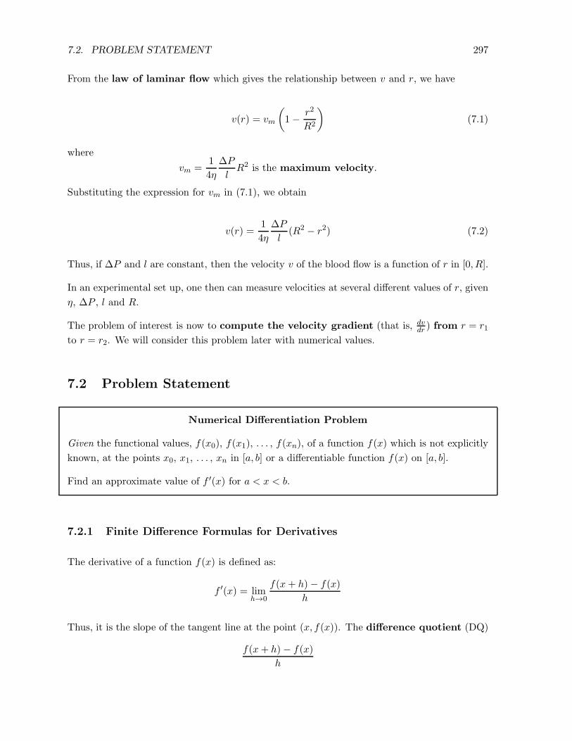
From the law of laminar flow which gives the relationship between v and r, we have
v(r) = vm
(
1− r2
R2
)
(7.1)
where
vm =1
4η
∆P
lR2 is the maximum velocity.
Substituting the expression for vm in (7.1), we obtain
v(r) =1
4η
∆P
l(R2 − r2) (7.2)
Thus, if ∆P and l are constant, then the velocity v of the blood flow is a function of r in [0, R].
In an experimental set up, one then can measure velocities at several different values of r, given
η, ∆P , l and R.
The problem of interest is now to compute the velocity gradient (that is, dvdr ) from r = r1
to r = r2. We will consider this problem later with numerical values.
7.2 Problem Statement
Numerical Differentiation Problem
Given the functional values, f(x0), f(x1), . . . , f(xn), of a function f(x) which is not explicitly
known, at the points x0, x1, . . . , xn in [a, b] or a differentiable function f(x) on [a, b].
Find an approximate value of f ′(x) for a < x < b.
7.2.1 Finite Difference Formulas for Derivatives
The derivative of a function f(x) is defined as:
f ′(x) = limh→0
f(x+ h)− f(x)
h
Thus, it is the slope of the tangent line at the point (x, f(x)). The difference quotient (DQ)
f(x+ h)− f(x)
h

298CHAPTER 7. NUMERICAL DIFFERENTIATION AND NUMERICAL INTEGRATION
is the slope of the secant line passing through (x, f(x)) and (x+ h, f(x+ h)).
(x, f(x))
(x+ h, f(x+ h))
x x+ h
As h gets smaller and smaller, the difference quotient gets closer and closer to f ′(x). However,
if h is too small, then the round-off error becomes large, yielding an inaccurate value of the
derivative.
In any case, if the DQ is taken as an approximate value of f ′(x), then it is called two-point
forward difference formula (FDF) for f ′(x).
Thus, two-point backward difference and two-point central difference formulas, are similarly
defined, respectively, in terms of the functional values f(x − h) and f(x), and f(x − h) and
f(x+ h).
Two-point Forward Difference Formula (FDF):
f ′(x) ≈ f(x+ h)− f(x)
h(7.3)
Two-point Backward Difference Formula (BDF):
f ′(x) ≈ f(x)− f(x− h)
h(7.4)
Two-point Central Difference Formula (CDF):
f ′(x) ≈ f(x+ h)− f(x)
h(7.5)
Example 7.1
Given the following table, where the functional values correspond to f(x) = x lnx:
x f(x)
1 0
2 1.3863
3 3.2958
7.2. PROBLEM STATEMENT 299
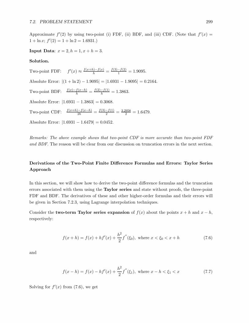
Approximate f ′(2) by using two-point (i) FDF, (ii) BDF, and (iii) CDF. (Note that f ′(x) =
1 + lnx; f ′(2) = 1 + ln 2 = 1.6931.)
Input Data: x = 2, h = 1, x+ h = 3.
Solution.
Two-point FDF: f ′(x) ≈ f(x+h)−f(x)h = f(3)−f(2)
1 = 1.9095.
Absolute Error: |(1 + ln 2)− 1.9095| = |1.6931 − 1.9095| = 0.2164.
Two-point BDF: f(x)−f(x−h)h = f(2)−f(1)
h = 1.3863.
Absolute Error: |1.6931 − 1.3863| = 0.3068.
Two-point CDF: f(x+h)−f(x−h)2h = f(3)−f(1)
2 = 3.29582 = 1.6479.
Absolute Error: |1.6931 − 1.6479| = 0.0452.
Remarks: The above example shows that two-point CDF is more accurate than two-point FDF
and BDF. The reason will be clear from our discussion on truncation errors in the next section.
Derivations of the Two-Point Finite Difference Formulas and Errors: Taylor Series
Approach
In this section, we will show how to derive the two-point difference formulas and the truncation
errors associated with them using the Taylor series and state without proofs, the three-point
FDF and BDF. The derivatives of these and other higher-order formulas and their errors will
be given in Section 7.2.3, using Lagrange interpolation techniques.
Consider the two-term Taylor series expansion of f(x) about the points x+ h and x− h,
respectively:
f(x+ h) = f(x) + hf ′(x) +h2
2f
′′
(ξ0), where x < ξ0 < x+ h (7.6)
and
f(x− h) = f(x)− hf ′(x) +h2
2f
′′
(ξ1), where x− h < ξ1 < x (7.7)
Solving for f ′(x) from (7.6), we get

300CHAPTER 7. NUMERICAL DIFFERENTIATION AND NUMERICAL INTEGRATION
f ′(x) =
[f(x+ h)− f(x)
h
]
− h
2f
′′
(ξ0) (7.8)
• The term within brackets on the right-hand side of (7.8) is the two-point FDF.
• The second term (remainder) on the right-hand side of (7.8) is the truncation error for
two-point FDF.
Similarly, solving for f ′(x) from (7.7), we get
f ′(x) =f(x)− f(x− h)
h+h
2f
′′
(ξ1) (7.9)
• The first term within brackets on the right-hand side of (7.9) is the two-point BDF.
• The second term (remainder) on the right-hand side of (7.9) is the truncation error for
two-point BDF.
Assume that f′′
(x) is continuous. Consider this time a three-term Taylor series expansion
of f(x) about the points (x+ h) and (x− h):
f(x+ h) = f(x) + hf ′(x) +h
2f
′′
(x) +h3
3!f
′′′
(ξ2) (7.10)
where x < ξ2 < x+ h, and
f(x− h) = f(x)− hf ′(x) +h2
2f
′′
(x)− h3
3!f
′′′
(ξ3) (7.11)
where x− h < ξ3 < x.
Subtracting (7.11) from (7.10), we obtain
f(x+ h)− f(x− h) = 2hf ′(x) +h3
3!
[
f′′′
(ξ2) + f′′′
(ξ3)]
(7.12)
Solving (7.12) for f ′(x), we get
f ′(x) =f(x+ h)− f(x− h)
2h− h2
12
[
f′′′
(ξ2) + f′′′
(ξ3)]
(7.13)
To simplify the expression within the brackets in (7.13), we need the following theorem from
Calculus:
7.2. PROBLEM STATEMENT 301
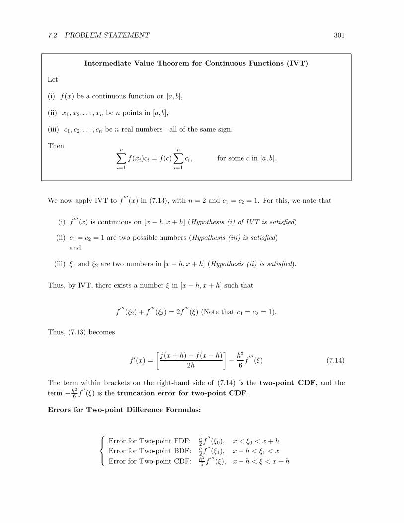
Intermediate Value Theorem for Continuous Functions (IVT)
Let
(i) f(x) be a continuous function on [a, b],
(ii) x1, x2, . . . , xn be n points in [a, b],
(iii) c1, c2, . . . , cn be n real numbers - all of the same sign.
Thenn∑
i=1
f(xi)ci = f(c)
n∑
i=1
ci, for some c in [a, b].
We now apply IVT to f′′′
(x) in (7.13), with n = 2 and c1 = c2 = 1. For this, we note that
(i) f′′′
(x) is continuous on [x− h, x+ h] (Hypothesis (i) of IVT is satisfied)
(ii) c1 = c2 = 1 are two possible numbers (Hypothesis (iii) is satisfied)
and
(iii) ξ1 and ξ2 are two numbers in [x− h, x+ h] (Hypothesis (ii) is satisfied).
Thus, by IVT, there exists a number ξ in [x− h, x+ h] such that
f′′′
(ξ2) + f′′′
(ξ3) = 2f′′′
(ξ) (Note that c1 = c2 = 1).
Thus, (7.13) becomes
f ′(x) =
[f(x+ h)− f(x− h)
2h
]
− h2
6f
′′′
(ξ) (7.14)
The term within brackets on the right-hand side of (7.14) is the two-point CDF, and the
term −h2
6 f′′
(ξ) is the truncation error for two-point CDF.
Errors for Two-point Difference Formulas:
Error for Two-point FDF: h2f
′′
(ξ0), x < ξ0 < x+ h
Error for Two-point BDF: h2f
′′
(ξ1), x− h < ξ1 < x
Error for Two-point CDF: h2
6 f′′′
(ξ), x− h < ξ < x+ h

302CHAPTER 7. NUMERICAL DIFFERENTIATION AND NUMERICAL INTEGRATION
Two-Point FDF and BDF Versus Two-Point CDF
• Two-point FDF and BDF are O(h) (they are first-order approximations).
• Two-point CDF are O(h2) (this is a second-order approximation).
It is now clear why two-point CDF is more accurate than both two-point FDF and BDF. This
is because, both two-point FDF and BDF are O(h) white two-point CDF is O(h2). Note that
Example 7.1 supports this statement.
7.2.2 Three-point and Higher Order Formulas for f ′(x): Lagrange Interpo-
lation Approach
Three-point and higher-order derivative formulas and their truncation errors can be derived in
the similar way as in the last section. Three-point FDF and BDF approximate f ′(x) in terms
of the functional values at three points: x, x+ h, and x+ 2h for FDF and x, x− h, x − 2h for
BDF, respectively.
Three-point FDF for f ′(x): f ′(x) ≈ −3f(x)+4f(x+h)−f(x+2h)2h
X −−−−−X −−−−−X
x x+ h x+ 2h
Three-point BDF for f ′(x): f ′(x) ≈ f(x−2h)−4f(x−h)+3f(x)2h
X −−−−−−−X −−−−−−−X
x− 2h x− h x
The derivations and error formulas of theses and other higher-order approximations are given
in the next section.
The difference formulas are simple to use but they are only good for approximating f ′(x) where
x is one of the tabulated points x0, x1, . . . , xn. On the other hand, if x is a nontabulated point
in [a, b], and f ′(x) is sought at that point, then the simplest thing to do is to:
• Find an interpolating polynomial Pn(x) passing through x0, x2, . . . , xn (we will use La-
grange interpolations here).
• Accept P′
n(x) as an approximation to f ′(x).
As we will see later, if x coincides with one of the points x0, x1, . . . , xn, then we can recover
some of the finite difference formulas of the last section, as special cases.
7.2. PROBLEM STATEMENT 303
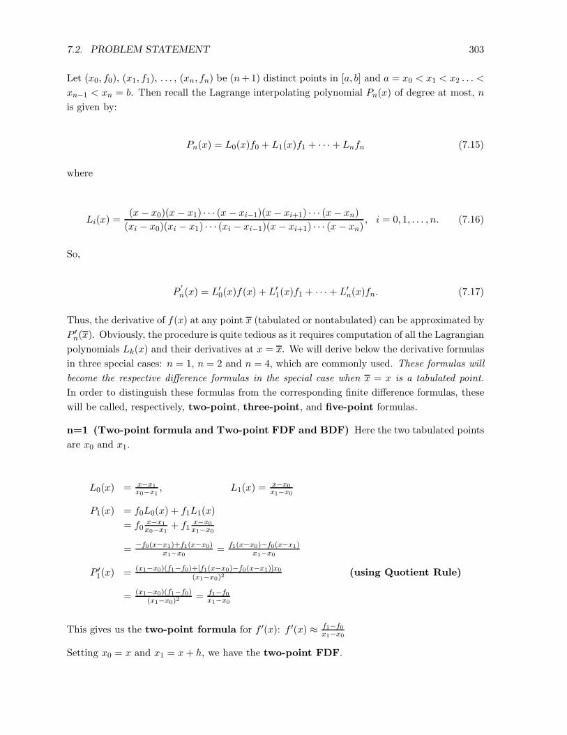
Let (x0, f0), (x1, f1), . . . , (xn, fn) be (n+1) distinct points in [a, b] and a = x0 < x1 < x2 . . . <
xn−1 < xn = b. Then recall the Lagrange interpolating polynomial Pn(x) of degree at most, n
is given by:
Pn(x) = L0(x)f0 + L1(x)f1 + · · ·+ Lnfn (7.15)
where
Li(x) =(x− x0)(x− x1) · · · (x− xi−1)(x− xi+1) · · · (x− xn)
(xi − x0)(xi − x1) · · · (xi − xi−1)(x− xi+1) · · · (x− xn), i = 0, 1, . . . , n. (7.16)
So,
P′
n(x) = L′0(x)f(x) + L′
1(x)f1 + · · · + L′n(x)fn. (7.17)
Thus, the derivative of f(x) at any point x (tabulated or nontabulated) can be approximated by
P ′n(x). Obviously, the procedure is quite tedious as it requires computation of all the Lagrangian
polynomials Lk(x) and their derivatives at x = x. We will derive below the derivative formulas
in three special cases: n = 1, n = 2 and n = 4, which are commonly used. These formulas will
become the respective difference formulas in the special case when x = x is a tabulated point.
In order to distinguish these formulas from the corresponding finite difference formulas, these
will be called, respectively, two-point, three-point, and five-point formulas.
n=1 (Two-point formula and Two-point FDF and BDF) Here the two tabulated points
are x0 and x1.
L0(x) = x−x1
x0−x1, L1(x) =
x−x0
x1−x0
P1(x) = f0L0(x) + f1L1(x)
= f0x−x1
x0−x1+ f1
x−x0
x1−x0
= −f0(x−x1)+f1(x−x0)x1−x0
= f1(x−x0)−f0(x−x1)x1−x0
P ′1(x) = (x1−x0)(f1−f0)+[f1(x−x0)−f0(x−x1)]x0
(x1−x0)2(using Quotient Rule)
= (x1−x0)(f1−f0)(x1−x0)2
= f1−f0x1−x0
This gives us the two-point formula for f ′(x): f ′(x) ≈ f1−f0x1−x0
Setting x0 = x and x1 = x+ h, we have the two-point FDF.
304CHAPTER 7. NUMERICAL DIFFERENTIATION AND NUMERICAL INTEGRATION
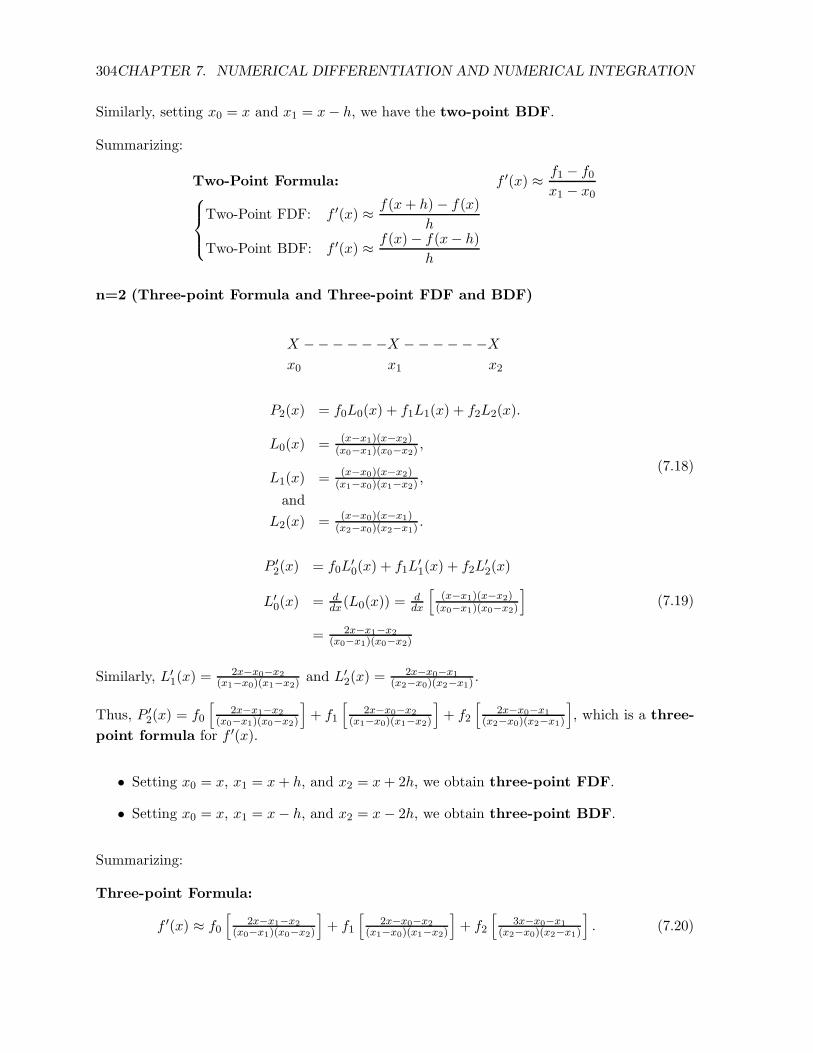
Similarly, setting x0 = x and x1 = x− h, we have the two-point BDF.
Summarizing:
Two-Point Formula: f ′(x) ≈ f1 − f0x1 − x0
Two-Point FDF: f ′(x) ≈ f(x+ h)− f(x)
h
Two-Point BDF: f ′(x) ≈ f(x)− f(x− h)
h
n=2 (Three-point Formula and Three-point FDF and BDF)
X −−−−−−X −−−−−−Xx0 x1 x2
P2(x) = f0L0(x) + f1L1(x) + f2L2(x).
L0(x) = (x−x1)(x−x2)(x0−x1)(x0−x2)
,
L1(x) = (x−x0)(x−x2)(x1−x0)(x1−x2)
,
and
L2(x) = (x−x0)(x−x1)(x2−x0)(x2−x1)
.
(7.18)
P ′2(x) = f0L
′0(x) + f1L
′1(x) + f2L
′2(x)
L′0(x) = d
dx(L0(x)) =ddx
[(x−x1)(x−x2)
(x0−x1)(x0−x2)
]
= 2x−x1−x2
(x0−x1)(x0−x2)
(7.19)
Similarly, L′1(x) =
2x−x0−x2
(x1−x0)(x1−x2)and L′
2(x) =2x−x0−x1
(x2−x0)(x2−x1).
Thus, P ′2(x) = f0
[2x−x1−x2
(x0−x1)(x0−x2)
]
+ f1
[2x−x0−x2
(x1−x0)(x1−x2)
]
+ f2
[2x−x0−x1
(x2−x0)(x2−x1)
]
, which is a three-
point formula for f ′(x).
• Setting x0 = x, x1 = x+ h, and x2 = x+ 2h, we obtain three-point FDF.
• Setting x0 = x, x1 = x− h, and x2 = x− 2h, we obtain three-point BDF.
Summarizing:
Three-point Formula:
f ′(x) ≈ f0
[2x−x1−x2
(x0−x1)(x0−x2)
]
+ f1
[2x−x0−x2
(x1−x0)(x1−x2)
]
+ f2
[3x−x0−x1
(x2−x0)(x2−x1)
]
. (7.20)
7.2. PROBLEM STATEMENT 305
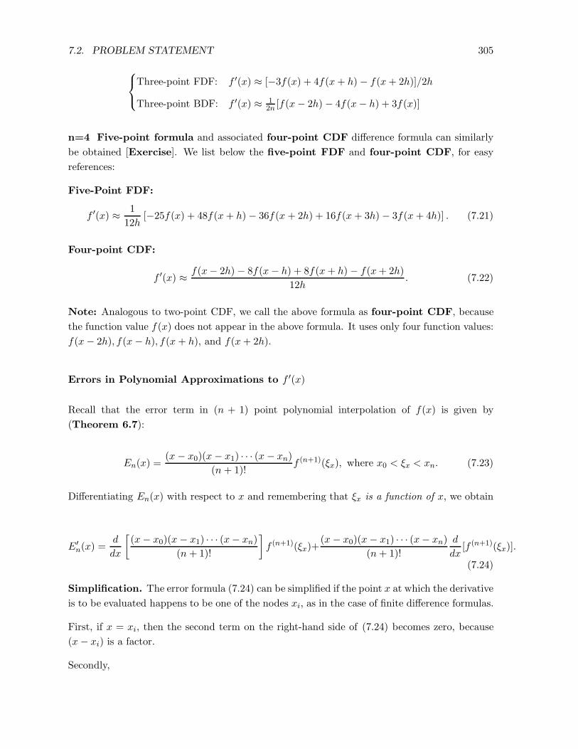
Three-point FDF: f ′(x) ≈ [−3f(x) + 4f(x+ h)− f(x+ 2h)]/2h
Three-point BDF: f ′(x) ≈ 12n [f(x− 2h) − 4f(x− h) + 3f(x)]
n=4 Five-point formula and associated four-point CDF difference formula can similarly
be obtained [Exercise]. We list below the five-point FDF and four-point CDF, for easy
references:
Five-Point FDF:
f ′(x) ≈ 1
12h[−25f(x) + 48f(x+ h)− 36f(x+ 2h) + 16f(x+ 3h)− 3f(x+ 4h)] . (7.21)
Four-point CDF:
f ′(x) ≈ f(x− 2h) − 8f(x− h) + 8f(x+ h)− f(x+ 2h)
12h. (7.22)
Note: Analogous to two-point CDF, we call the above formula as four-point CDF, because
the function value f(x) does not appear in the above formula. It uses only four function values:
f(x− 2h), f(x− h), f(x+ h), and f(x+ 2h).
Errors in Polynomial Approximations to f ′(x)
Recall that the error term in (n + 1) point polynomial interpolation of f(x) is given by
(Theorem 6.7):
En(x) =(x− x0)(x− x1) · · · (x− xn)
(n + 1)!f (n+1)(ξx), where x0 < ξx < xn. (7.23)
Differentiating En(x) with respect to x and remembering that ξx is a function of x, we obtain
E′n(x) =
d
dx
[(x− x0)(x− x1) · · · (x− xn)
(n + 1)!
]
f (n+1)(ξx)+(x− x0)(x− x1) · · · (x− xn)
(n+ 1)!
d
dx[f (n+1)(ξx)].
(7.24)
Simplification. The error formula (7.24) can be simplified if the point x at which the derivative
is to be evaluated happens to be one of the nodes xi, as in the case of finite difference formulas.
First, if x = xi, then the second term on the right-hand side of (7.24) becomes zero, because
(x− xi) is a factor.
Secondly,
306CHAPTER 7. NUMERICAL DIFFERENTIATION AND NUMERICAL INTEGRATION
d
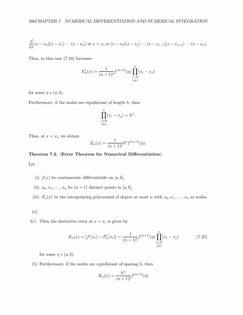
dx(x−x0)(x−x1) · · · (x−xn) at x = xi is (x−x0)(x−x1) · · · (x−xi−1)(x−xi+1) · · · (x−xn).
Thus, in this case (7.24) becomes
E′n(x) =
1
(n+ 1)!f (n+1)(η)
n∏
j=0j 6=i
(xi − xj)
for some η ǫ (a, b).
Furthermore, if the nodes are equidistant of length h, then
n∏
j=0i 6=j
(xi − xj) = hn.
Thus, at x = xi, we obtain
En(x) =1
(n + 1)!hnf (n+1)(η).
Theorem 7.2. (Error Theorem for Numerical Differentiation).
Let
(i) f(x) be continuously differentiable on [a, b],
(ii) x0, x1, . . . , xn be (n+ 1) distinct points in [a, b],
(iii) Pn(x) be the interpolating polynomial of degree at most n with x0, x1, . . . , xn as nodes.
(a)
6.1. Then the derivative error at x = xi is given by
En(x) =∣∣f ′(xi)− P ′
n(xi)∣∣ =
1
(n+ 1)!f (n+1)(η)
n∏
j=0j 6=i
(xi − xj) (7.25)
for some η ǫ (a, b).
(b) Furthermore, if the nodes are equidistant of spacing h, then
En(x) =hn
(n+ 1)!f (n+1)(η)
7.2. PROBLEM STATEMENT 307
Special cases: Since finite difference formulas concern finding the derivative at a tabulated
point, x = xi, we immediately recover the following error results established earlier:
• Two-point FDF and BDF (n = 1) are O(h). (First-order approximation)
• Two-point CDF and three-point FDF and BDF (n = 2) are O(h2). (Second-order
approximation)
• Four-point CDF and five-point FDF and BDF (n = 3) are O(h3). (Third-order ap-
proximation)
and so on.
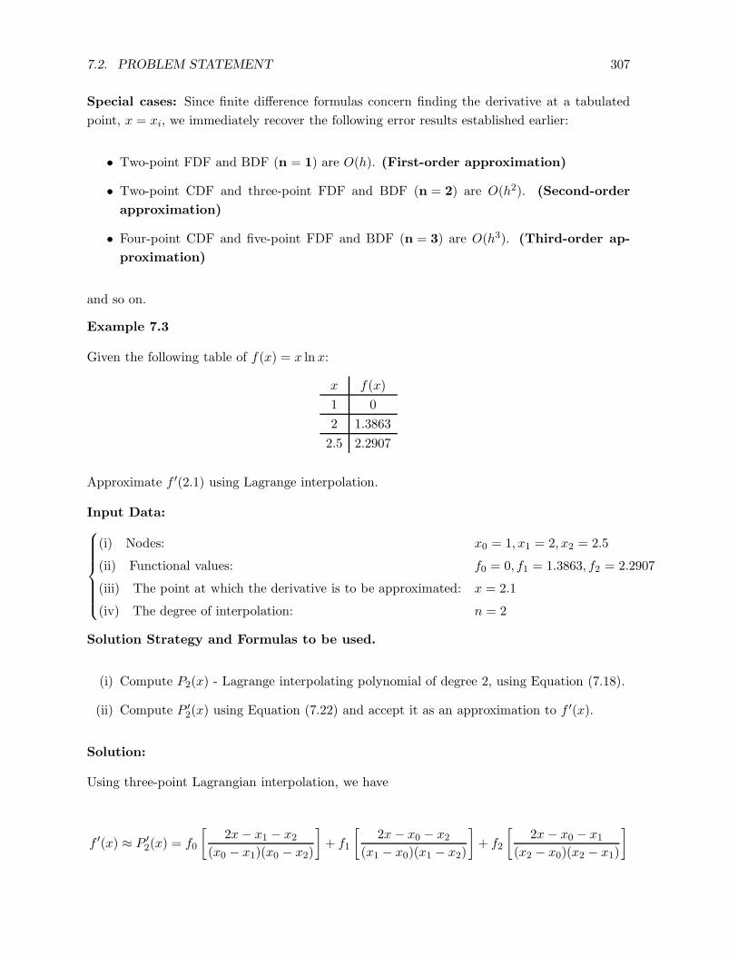
Example 7.3
Given the following table of f(x) = x lnx:
x f(x)
1 0
2 1.3863
2.5 2.2907
Approximate f ′(2.1) using Lagrange interpolation.
Input Data:
(i) Nodes: x0 = 1, x1 = 2, x2 = 2.5
(ii) Functional values: f0 = 0, f1 = 1.3863, f2 = 2.2907
(iii) The point at which the derivative is to be approximated: x = 2.1
(iv) The degree of interpolation: n = 2
Solution Strategy and Formulas to be used.
(i) Compute P2(x) - Lagrange interpolating polynomial of degree 2, using Equation (7.18).
(ii) Compute P ′2(x) using Equation (7.22) and accept it as an approximation to f ′(x).
Solution:
Using three-point Lagrangian interpolation, we have
f ′(x) ≈ P ′2(x) = f0
[2x− x1 − x2
(x0 − x1)(x0 − x2)
]
+ f1
[2x− x0 − x2
(x1 − x0)(x1 − x2)
]
+ f2
[2x− x0 − x1
(x2 − x0)(x2 − x1)
]
308CHAPTER 7. NUMERICAL DIFFERENTIATION AND NUMERICAL INTEGRATION
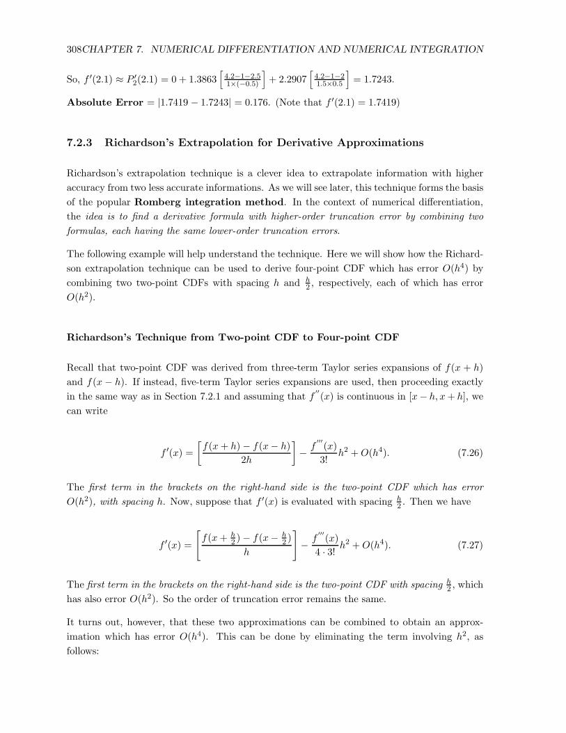
So, f ′(2.1) ≈ P ′2(2.1) = 0 + 1.3863
[4.2−1−2.51×(−0.5)
]
+ 2.2907[4.2−1−21.5×0.5
]
= 1.7243.
Absolute Error = |1.7419 − 1.7243| = 0.176. (Note that f ′(2.1) = 1.7419)
7.2.3 Richardson’s Extrapolation for Derivative Approximations
Richardson’s extrapolation technique is a clever idea to extrapolate information with higher
accuracy from two less accurate informations. As we will see later, this technique forms the basis
of the popular Romberg integration method. In the context of numerical differentiation,
the idea is to find a derivative formula with higher-order truncation error by combining two
formulas, each having the same lower-order truncation errors.
The following example will help understand the technique. Here we will show how the Richard-
son extrapolation technique can be used to derive four-point CDF which has error O(h4) by
combining two two-point CDFs with spacing h and h2 , respectively, each of which has error
O(h2).
Richardson’s Technique from Two-point CDF to Four-point CDF
Recall that two-point CDF was derived from three-term Taylor series expansions of f(x + h)
and f(x− h). If instead, five-term Taylor series expansions are used, then proceeding exactly
in the same way as in Section 7.2.1 and assuming that f′′
(x) is continuous in [x− h, x+ h], we
can write
f ′(x) =
[f(x+ h)− f(x− h)
2h
]
− f′′′
(x)
3!h2 +O(h4). (7.26)
The first term in the brackets on the right-hand side is the two-point CDF which has error
O(h2), with spacing h. Now, suppose that f ′(x) is evaluated with spacing h2 . Then we have
f ′(x) =
[
f(x+ h2 )− f(x− h
2 )
h
]
− f′′′
(x)
4 · 3! h2 +O(h4). (7.27)
The first term in the brackets on the right-hand side is the two-point CDF with spacing h2 , which
has also error O(h2). So the order of truncation error remains the same.
It turns out, however, that these two approximations can be combined to obtain an approx-
imation which has error O(h4). This can be done by eliminating the term involving h2, as
follows:
7.2. PROBLEM STATEMENT 309
First, multiply Equation (7.27) by 4 to obtain
4f ′(x) = 4f(x+ h
2 )− f(x− h2 )
h− f
′′
(x)
3!h2 +O(h4).
Next, subtract the last equation from Equation (7.26) and divide the result by 3, yielding
f ′(x) =1
3
[
4f(x+ h
2 )− f(x− h)
h− f(x+ h)− f(x− h)
2h
]
+O(h4).
This is an approximation of f ′(x) with error O(h4). Indeed, the reader will easily recognize the
term in the bracket on the right-hand side, as the four-point CDF with spacing h2 ; that is with
the points: x− h, x− h2 , x, x+ h
2 , x+ h. Replacing h by 2h in the above formula, we have
f ′(x) ≈ 8f(x+ h)− 8f(x− h)− f(x+ 2h) + f(x− 2h)
12h(7.28)
which is the four-point CDF with spacing h and we already know that this approximation has
error O(h4).
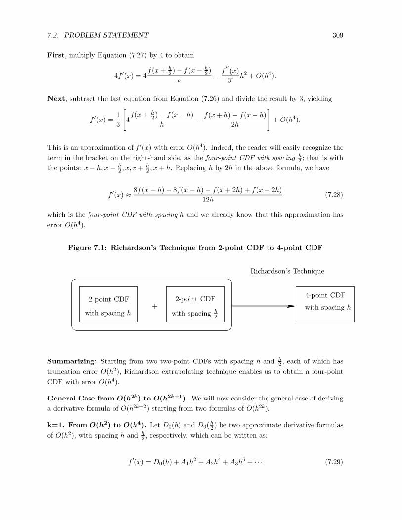
2-point CDF
with spacing h+
2-point CDF
with spacing h2
Richardson’s Technique
4-point CDF
with spacing h
Figure 7.1: Richardson’s Technique from 2-point CDF to 4-point CDF
Summarizing: Starting from two two-point CDFs with spacing h and h2 , each of which has
truncation error O(h2), Richardson extrapolating technique enables us to obtain a four-point
CDF with error O(h4).
General Case from O(h2k) to O(h2k+1). We will now consider the general case of deriving
a derivative formula of O(h2k+2) starting from two formulas of O(h2k).
k=1. From O(h2) to O(h4). Let D0(h) and D0(h2 ) be two approximate derivative formulas
of O(h2), with spacing h and h2 , respectively, which can be written as:
f ′(x) = D0(h) +A1h2 +A2h
4 +A3h6 + · · · (7.29)

310CHAPTER 7. NUMERICAL DIFFERENTIATION AND NUMERICAL INTEGRATION
f ′(x) = D0
(h
2
)
+A1
(h
2
)2
+A2
(h
2
)4
+A3
(h
2
)6
+ · · · , (7.30)
where A1, A2, A3, etc. are constants independent of h.
As in the last section, a formula of O(h4) can now be obtained by eliminating two terms
involving h2 from the above two equations. This is done as follows:
Subtract (7.29) from 4×(7.30) to obtain:
3f ′(x) = 4D0(h2 )−D0(h) − 3
4A2h4 + · · ·
or f ′(x) = 43D0(
h2 )− 1
3D0(h) − 14A2h
4 + · · ·
or f ′(x) = D0(h2 ) +
D0(h
2)−D0(h)
3 − 14A2h
4 + · · ·
Set D1(h) = D0(h2 ) +
D0(h
2)−D0(h)
3 .
Then f ′(x) = D1(h)− 14A2h
4 + · · ·
(7.31)
Thus, D1(h) is an O(h4) approximation of f ′(x).
k=2. From O(h4) to O(h6). To start with, we have f ′(x) = D1(h)− 14A2h
4 + · · · .
Replace h by h2 to obtain
f ′(x) = D1
(h
2
)
− 1
4A2
(h
2
)4
+ · · · (7.32)
To obtain an O(h6) approximation, subtract (7.29) from 16×(7.30) to obtain
15f ′(x) = 16D1(h2 )−D1(h) +O(h6)
or f ′(x) = 1615D1(
h2 )− 1
15D1(h) +O(h6)
= D1(h2 ) +
D1(h
2)−D1(h)
15 +O(h6)
Set D2(h) = D1(h2 ) +
D1(h
2)−D1(h)
15
So, f ′(x) = D2(h) +O(h6).
(7.33)
Thus, D2(h) is an O(h6) approximation of f ′(x).
7.2. PROBLEM STATEMENT 311
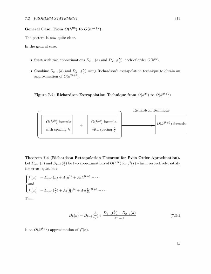
General Case: From O(h2k) to O(h2k+2).
The pattern is now quite clear.
In the general case,
• Start with two approximations Dk−1(h) and Dk−1(h2 ), each of order O(h2k).
• Combine Dk−1(h) and Dk−1(h2 ) using Richardson’s extrapolation technique to obtain an
approximation of O(h2k+2).
O(h2k) formula
with spacing h+
O(h2k) formula
with spacing h2
Richardson Technique
O(h2k+2) formula
Figure 7.2: Richardson Extrapolation Technique from O(h2k) to O(h2k+2)
Theorem 7.4 (Richardson Extrapolation Theorem for Even Order Aproximation).
Let Dk−1(h) andDk−1(h2 ) be two approximations of O(h2k) for f ′(x) which, respectively, satisfy
the error equations:
f ′(x) = Dk−1(h) +A1h2k +A2h
2k+2 + · · ·and
f ′(x) = Dk−1(h2 ) +A1(
h2 )
2k +A2(h2 )
2k+2 + · · ·
Then
Dk(h) = Dk−1(h
2) +
Dk−1(h2 )−Dk−1(h)
4k − 1(7.34)
is an O(h2k+2) approximation of f ′(x).
�
312CHAPTER 7. NUMERICAL DIFFERENTIATION AND NUMERICAL INTEGRATION
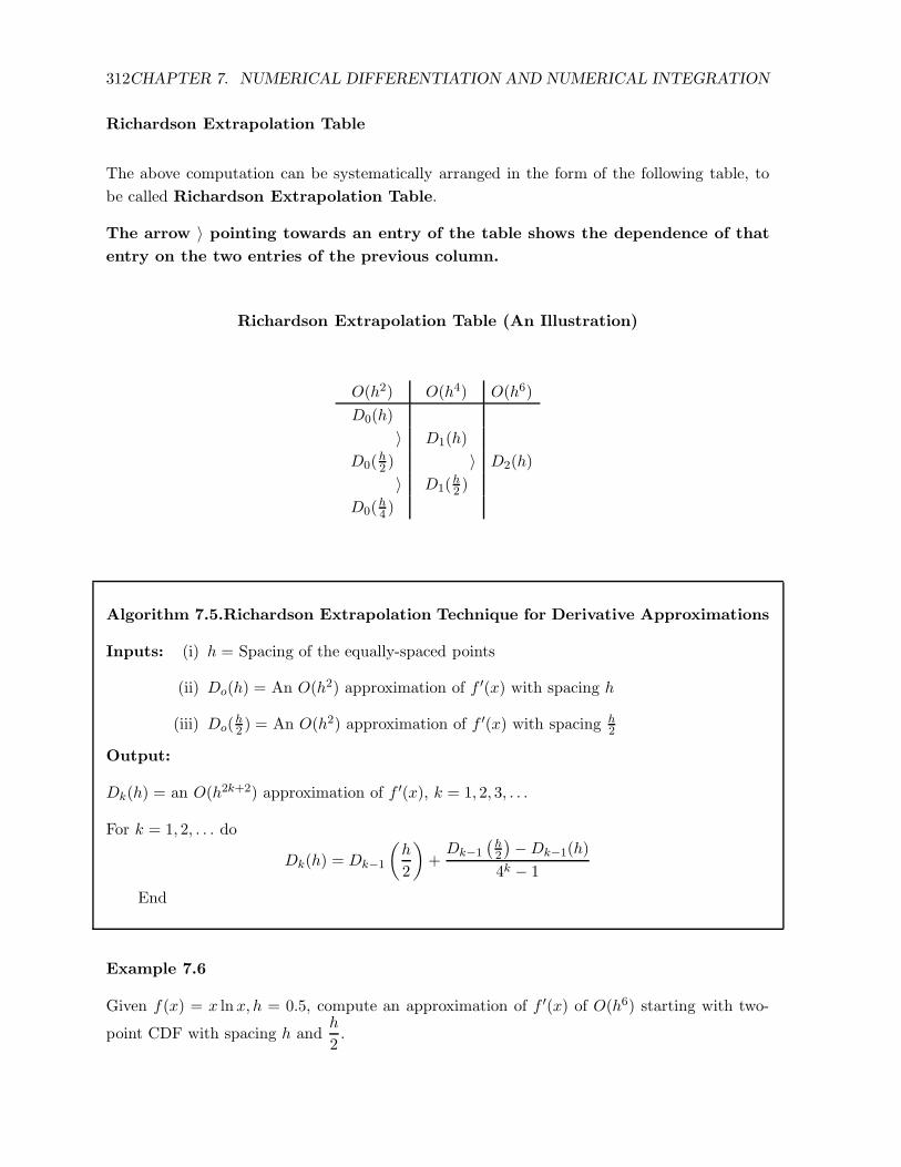
Richardson Extrapolation Table
The above computation can be systematically arranged in the form of the following table, to
be called Richardson Extrapolation Table.
The arrow 〉 pointing towards an entry of the table shows the dependence of that
entry on the two entries of the previous column.
Richardson Extrapolation Table (An Illustration)
O(h2) O(h4) O(h6)
D0(h)
〉 D1(h)
D0(h2 ) 〉 D2(h)
〉 D1(h2 )
D0(h4 )
Algorithm 7.5.Richardson Extrapolation Technique for Derivative Approximations
Inputs: (i) h = Spacing of the equally-spaced points
(ii) Do(h) = An O(h2) approximation of f ′(x) with spacing h
(iii) Do(h2 ) = An O(h2) approximation of f ′(x) with spacing h
2
Output:
Dk(h) = an O(h2k+2) approximation of f ′(x), k = 1, 2, 3, . . .
For k = 1, 2, . . . do
Dk(h) = Dk−1
(h
2
)
+Dk−1
(h2
)−Dk−1(h)
4k − 1
End
Example 7.6
Given f(x) = x lnx, h = 0.5, compute an approximation of f ′(x) of O(h6) starting with two-
point CDF with spacing h andh
2.
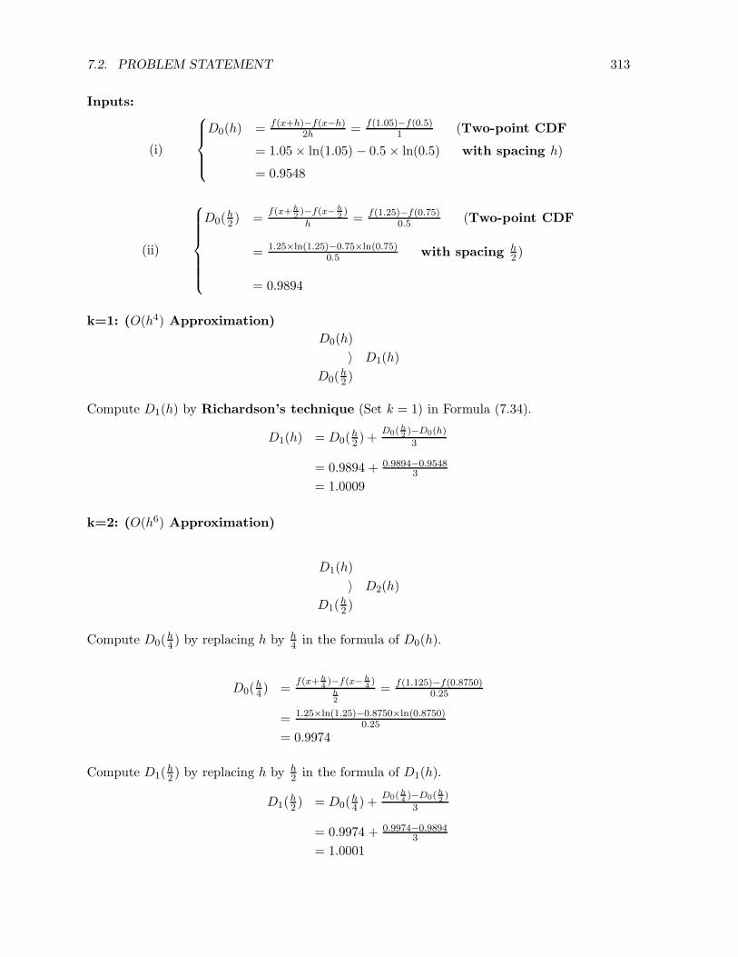
7.2. PROBLEM STATEMENT 313
Inputs:
(i)
D0(h) = f(x+h)−f(x−h)2h = f(1.05)−f(0.5)
1 (Two-point CDF
= 1.05× ln(1.05) − 0.5 × ln(0.5) with spacing h)
= 0.9548
(ii)
D0(h2 ) =
f(x+h
2)−f(x−h
2)
h = f(1.25)−f(0.75)0.5 (Two-point CDF
= 1.25×ln(1.25)−0.75×ln(0.75)0.5 with spacing h
2 )
= 0.9894
k=1: (O(h4) Approximation)
D0(h)
〉 D1(h)
D0(h2 )
Compute D1(h) by Richardson’s technique (Set k = 1) in Formula (7.34).
D1(h) = D0(h2 ) +
D0(h
2)−D0(h)
3
= 0.9894 + 0.9894−0.95483
= 1.0009
k=2: (O(h6) Approximation)
D1(h)
〉 D2(h)
D1(h2 )
Compute D0(h4 ) by replacing h by h
4 in the formula of D0(h).
D0(h4 ) =
f(x+h
4)−f(x−h
4)
h
2
= f(1.125)−f(0.8750)0.25
= 1.25×ln(1.25)−0.8750×ln(0.8750)0.25
= 0.9974
Compute D1(h2 ) by replacing h by h
2 in the formula of D1(h).
D1(h2 ) = D0(
h4 ) +
D0(h
4)−D0(
h
2)
3
= 0.9974 + 0.9974−0.98943
= 1.0001
314CHAPTER 7. NUMERICAL DIFFERENTIATION AND NUMERICAL INTEGRATION
Compute D2(h) by Richardson’s technique (set k = 2) in Formula (7.34).
D2(h) = D1(h2 ) +
D1(h
2)−D1(h)
15
= 1.0000
Richardson Extrapolation Table for Example 7.4:
O(h2) O(h4) O(h6)
0.9548
0.9894 1.0009 1.0000
0.9974 1.0001
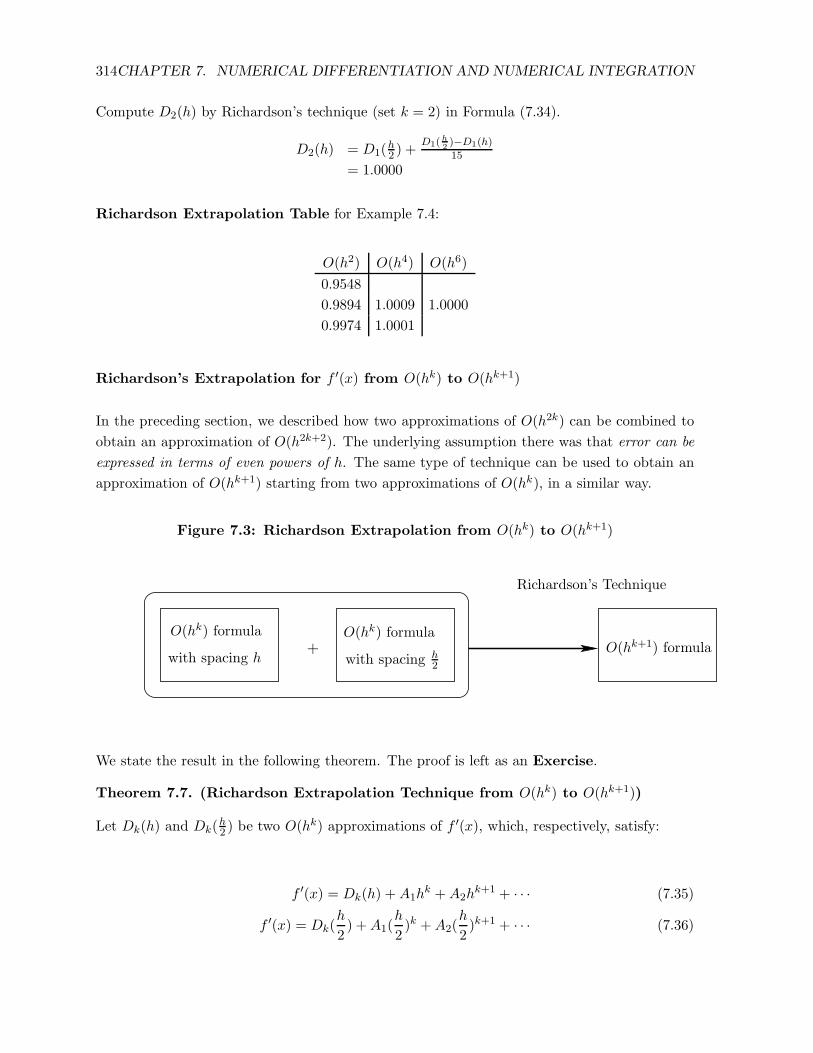
Richardson’s Extrapolation for f ′(x) from O(hk) to O(hk+1)
In the preceding section, we described how two approximations of O(h2k) can be combined to
obtain an approximation of O(h2k+2). The underlying assumption there was that error can be
expressed in terms of even powers of h. The same type of technique can be used to obtain an
approximation of O(hk+1) starting from two approximations of O(hk), in a similar way.
O(hk) formula
with spacing h+
O(hk) formula
with spacing h2
Richardson’s Technique
O(hk+1) formula
Figure 7.3: Richardson Extrapolation from O(hk) to O(hk+1)
We state the result in the following theorem. The proof is left as an Exercise.
Theorem 7.7. (Richardson Extrapolation Technique from O(hk) to O(hk+1))
Let Dk(h) and Dk(h2 ) be two O(hk) approximations of f ′(x), which, respectively, satisfy:
f ′(x) = Dk(h) +A1hk +A2h
k+1 + · · · (7.35)
f ′(x) = Dk(h
2) +A1(
h
2)k +A2(
h
2)k+1 + · · · (7.36)
7.2. PROBLEM STATEMENT 315
Then
Dk(h) = Dk−1(h
2) +
Dk−1(h2 )−Dk−1(h)
2k−1 − 1, k = 2, 3, 4, . . . (7.37)
is an O(hk+1) approximation of f ′(x).
�
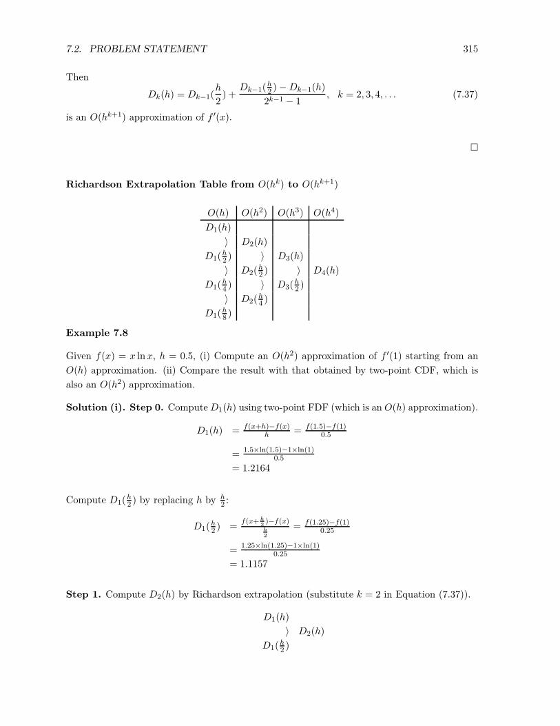
Richardson Extrapolation Table from O(hk) to O(hk+1)
O(h) O(h2) O(h3) O(h4)
D1(h)
〉 D2(h)
D1(h2 ) 〉 D3(h)
〉 D2(h2 ) 〉 D4(h)
D1(h4 ) 〉 D3(
h2 )
〉 D2(h4 )
D1(h8 )
Example 7.8
Given f(x) = x lnx, h = 0.5, (i) Compute an O(h2) approximation of f ′(1) starting from an
O(h) approximation. (ii) Compare the result with that obtained by two-point CDF, which is
also an O(h2) approximation.
Solution (i). Step 0. ComputeD1(h) using two-point FDF (which is an O(h) approximation).
D1(h) = f(x+h)−f(x)h = f(1.5)−f(1)
0.5
= 1.5×ln(1.5)−1×ln(1)0.5
= 1.2164
Compute D1(h2 ) by replacing h by h
2 :
D1(h2 ) =
f(x+h
2)−f(x)h
2
= f(1.25)−f(1)0.25
= 1.25×ln(1.25)−1×ln(1)0.25
= 1.1157
Step 1. Compute D2(h) by Richardson extrapolation (substitute k = 2 in Equation (7.37)).
D1(h)
〉 D2(h)
D1(h2 )
316CHAPTER 7. NUMERICAL DIFFERENTIATION AND NUMERICAL INTEGRATION
D2(h) = D1(h2 ) +
D1(h
2)−D1(h)
2−1
= 1.1157 + 1.1157−1.21641
= 1.0150
Absolute Error: |1.0150 − 1| = 0.0150. (Note that f ′(1) = 1).
Note: D1(h) and D1(h2 ) are of O(h) and D2(h) is of O(h2).
Solution (ii). Comparison with Two-Point CDF:
Two-point CDF = f(x+h)−f(x−h)2h = f(1.5)−f(0.5)
2×0.5
= 1.5×ln(1.5)−0.5×ln(0.5)1
= 0.9548
Absolute Error: |0.9548 − 1| = 0.0452.
Clearly, an O(h2) Richardson extrapolation technique is more accurate than two-point CDF,
which is also O(h2).
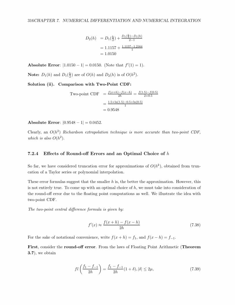
7.2.4 Effects of Round-off Errors and an Optimal Choice of h
So far, we have considered truncation error for approximations of O(hk), obtained from trun-
cation of a Taylor series or polynomial interpolation.
These error formulas suggest that the smaller h is, the better the approximation. However, this
is not entirely true. To come up with an optimal choice of h, we must take into consideration of
the round-off error due to the floating point computations as well. We illustrate the idea with
two-point CDF.
The two-point central difference formula is given by:
f ′(x) ≈ f(x+ h)− f(x− h)
2h(7.38)
For the sake of notational convenience, write f(x+ h) = f1, and f(x− h) = f−1.
First, consider the round-off error. From the laws of Floating Point Arithmetic (Theorem
3.7), we obtain
fl
(f1 − f−1
2h
)
=f1 − f−1
2h(1 + δ), |δ| ≤ 2µ, (7.39)

7.2. PROBLEM STATEMENT 317
where µ is the machine precision. Thus, round-off error in computing the CDF ≤ µh .
Next, let’s consider the truncation error. Assume that |f (3)(x)| ≤M . Then from (7.17), we
obtain the truncation error for two CDF’s is ≤M h2
6 .
So, the total error (absolute) = round-off error + truncation error ≤ µh +M h2
6 .
Significance of this result is the following:
Though h2
6 becomes smaller as h becomes smaller, the contribution from the round-off error, µh ,
becomes larger as h becomes smaller. Eventually, when h is too small, the large round-off
error will dominate and the computation will become inaccurate.
This simple illustration reveals the fact that too small of a value of h is hardly an advantage.
What is important is how to choose a value of h that will minimize the total error.
Choosing an optimal h
Since the maximum total absolute error
E(h) =µ
h+h2
6M
is a function of h, an optimal value of h may be obtained by minimizing E(h), assuming of
course, one can find the upper boundM for f′′′
(x). We give a simple example to illustrate this.
Example 7.9
Given f(x) = ex, 0 ≤ x ≤ 1. Find the optimal value of h for which the total error in computing
two-point CDF approximation to f ′(x) will be as small as possible.
Solution. We need to find h for which the maximum absolute total error (which is a function
of h):
E(h) =µ
h+M
h2
6
will be minimized.
Find M :f(x) = ex f (3)(x) = ex
|f (3)(x)| ≤ |ex| ≤ e in 0 ≤ x ≤ 1
So, M = e
Thus, |E(h)| ≤ µh + eµ
2
6 .
318CHAPTER 7. NUMERICAL DIFFERENTIATION AND NUMERICAL INTEGRATION
Minimize E(h).
E(h) =µ
h+ e
h2
6
is a simple function of h. It is easy to see that E(h) will be minimized if h = 3
√3µe . Assume
now µ = 2× 10⁻⁷ (single-precision). Then E(h) will be minimized if
h =3
√
3× 2× 10−7
e≈ 0.0060
Verification. The readers are invited to verify [Exercise] the above result by computing
errors with different values of h in the neighborhood of 0.0060.
7.2.5 Approximations of Higher-order Derivatives and Partial Derivatives
Needs for computing higher-order and partial derivatives arises in a wide variety of scientific
and engineering applications. Mathematical models of many of these applications are either
second- or higher-order differential equations and/or partial differential equations. Typically,
such equations are solved in two stages:
Stage I The differential equations are approximated by means of finite differences or finite
element techniques that lead to a system of algebraic equations.
Stage II Solution to the system of algebraic equations gives the solution of the applied problem.
We will consider finite difference approximation of second-order derivatives and first- and
second-order partial derivatives. These formulas can be derived exactly in the same way as
their counterparts for the first-order derivatives. We will illustrate the derivation of three-
point difference formulas for f′′
(x).
Three-Point Difference Formulas for Second Derivatives and their Truncation Er-
rors
Suppose that the functional values of x, x+h, and x+2h are known. Using three-term Taylor’s
series expansion of f(x+ h) with error terms, we can write
f(x+ h) = f(x) + hf ′(x) +h2
2!f
′′
(x) +h3
3!f
′′
(ξ1) where x < ξ1 < x+ h. (7.40)
Similarly,
f(x+ 2h) = f(x) + 2hf ′(x) +4h2
2!f
′′
(x) +8h3
3!f
′′
(ξ2) where x < ξ1 < x+ 2h. (7.41)

7.2. PROBLEM STATEMENT 319
Eliminate now f ′(x) from these two equations. To do this, multiply Equation (7.40) by 2 and
subtract it from Equation (7.41),
f(x+ 2h) − 2f(x+ h) = −f(x) + h2f′′
(x) + h3(f′′
(ξ2)− f′′
(ξ1)) (7.42)
Assuming that f′′′
(x) is continuous on [x, x + 2h], by the Intermediate Value Theorem,
there exists a number ξ between ξ1 and ξ2 such that
f′′
(x) =f
′′′
(ξ1) + f′′′
(ξ2)
2. (7.43)
Thus, we have
f(x+ 2h) − 2f(x+ h) = −f(x) + h2f′′
(x) +h3
2f
′′
(ξ) (7.44)
Solving for f′′
(x), we have the three-point FDF for f′′
(x).
In the same way, we can derive three-point BDF and CDF, and other higher-order formulas for
f′′
(x). We state some of these formulas below. Their derivations are left as Exercises.
Three-point FDF for f′′
(x) with Error Term:
f′′
(x) =f(x)− 2f(x+ h) + f(x+ 2h)
h2+h
2f
′′
(ξ) (7.45)
Three-point BDF for f′′
(x) with Error Term:
f′′
(x) =f(x− 2h)− 2f(x− h) + f(x)
h2+O(h) (7.46)
Three-point CDF for f′′
(x) with Error Term:
f′′
(x) =1
h2[f(x− h)− 2f(x) + f(x+ h)]− h2
12f4(ξ), where x− h < ξ < x+ h. (7.47)
Five-point CDF for f′′
(x) with Error Term:
f′′
(x) =−f(x− 2h) + 16f(x− h)− 30f(x) + 16f(x+ h)− f(x+ 2h)
12h2+O(h4) (7.48)
Example 7.10
For the function f(x) = x lnx, approximate f′′
(x) at x = 1, using the five-point forward
difference formula, with h = 0.1.
320CHAPTER 7. NUMERICAL DIFFERENTIATION AND NUMERICAL INTEGRATION
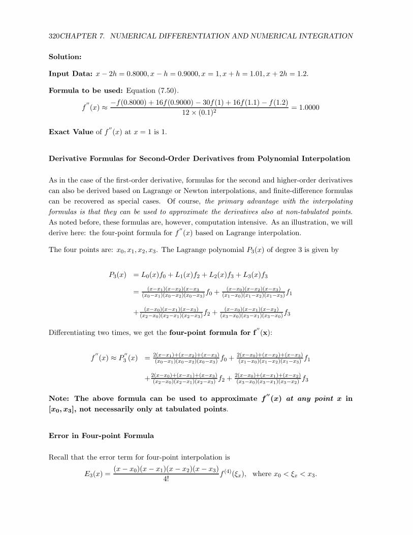
Solution:
Input Data: x− 2h = 0.8000, x − h = 0.9000, x = 1, x+ h = 1.01, x + 2h = 1.2.
Formula to be used: Equation (7.50).
f′′
(x) ≈ −f(0.8000) + 16f(0.9000) − 30f(1) + 16f(1.1) − f(1.2)
12 × (0.1)2= 1.0000
Exact Value of f′′
(x) at x = 1 is 1.
Derivative Formulas for Second-Order Derivatives from Polynomial Interpolation
As in the case of the first-order derivative, formulas for the second and higher-order derivatives
can also be derived based on Lagrange or Newton interpolations, and finite-difference formulas
can be recovered as special cases. Of course, the primary advantage with the interpolating
formulas is that they can be used to approximate the derivatives also at non-tabulated points.
As noted before, these formulas are, however, computation intensive. As an illustration, we will
derive here: the four-point formula for f′′
(x) based on Lagrange interpolation.
The four points are: x0, x1, x2, x3. The Lagrange polynomial P3(x) of degree 3 is given by
P3(x) = L0(x)f0 + L1(x)f2 + L2(x)f3 + L3(x)f3
= (x−x1)(x−x2)(x−x3
(x0−x1)(x0−x2)(x0−x3)f0 +
(x−x0)(x−x2)(x−x3)(x1−x0)(x1−x2)(x1−x3)
f1
+ (x−x0)(x−x1)(x−x3)(x2−x0)(x2−x1)(x2−x3)
f2 +(x−x0)(x−x1)(x−x2)
(x3−x0)(x3−x1)(x3−x0)f3
Differentiating two times, we get the four-point formula for f′′
(x):
f′′
(x) ≈ P′′
3 (x) = 2(x−x1)+(x−x2)+(x−x3)(x0−x1)(x0−x2)(x0−x3)
f0 +2(x−x0)+(x−x2)+(x−x3)(x1−x0)(x1−x2)(x1−x3)
f1
+2(x−x0)+(x−x1)+(x−x3)(x2−x0)(x2−x1)(x2−x3)
f2 +2(x−x0)+(x−x1)+(x−x2)(x3−x0)(x3−x1)(x3−x2)
f3
Note: The above formula can be used to approximate f′′
(x) at any point x in
[x0, x3], not necessarily only at tabulated points.
Error in Four-point Formula
Recall that the error term for four-point interpolation is
E3(x) =(x− x0)(x− x1)(x− x2)(x− x3)
4!f (4)(ξx), where x0 < ξx < x3.
7.2. PROBLEM STATEMENT 321
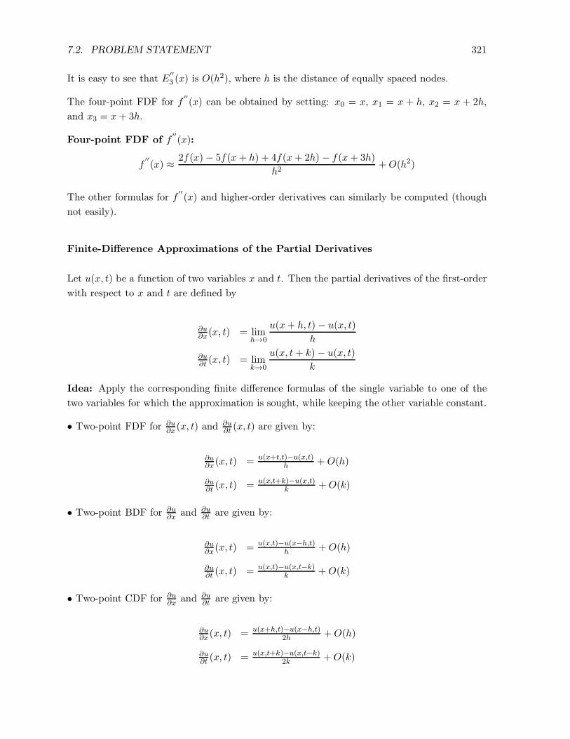
It is easy to see that E′′
3 (x) is O(h2), where h is the distance of equally spaced nodes.
The four-point FDF for f′′
(x) can be obtained by setting: x0 = x, x1 = x + h, x2 = x + 2h,
and x3 = x+ 3h.
Four-point FDF of f′′
(x):
f′′
(x) ≈ 2f(x)− 5f(x+ h) + 4f(x+ 2h)− f(x+ 3h)
h2+O(h2)
The other formulas for f′′
(x) and higher-order derivatives can similarly be computed (though
not easily).
Finite-Difference Approximations of the Partial Derivatives
Let u(x, t) be a function of two variables x and t. Then the partial derivatives of the first-order
with respect to x and t are defined by
∂u∂x(x, t) = lim
h→0
u(x+ h, t) − u(x, t)
h
∂u∂t (x, t) = lim
k→0
u(x, t+ k)− u(x, t)
k
Idea: Apply the corresponding finite difference formulas of the single variable to one of the
two variables for which the approximation is sought, while keeping the other variable constant.
• Two-point FDF for ∂u∂x(x, t) and
∂u∂t (x, t) are given by:
∂u∂x(x, t) = u(x+t,t)−u(x,t)
h +O(h)
∂u∂t (x, t) = u(x,t+k)−u(x,t)
k +O(k)
• Two-point BDF for ∂u∂x and ∂u
∂t are given by:
∂u∂x(x, t) = u(x,t)−u(x−h,t)
h +O(h)
∂u∂t (x, t) = u(x,t)−u(x,t−k)
k +O(k)
• Two-point CDF for ∂u∂x and ∂u
∂t are given by:
∂u∂x(x, t) = u(x+h,t)−u(x−h,t)
2h +O(h)
∂u∂t (x, t) = u(x,t+k)−u(x,t−k)
2k +O(k)
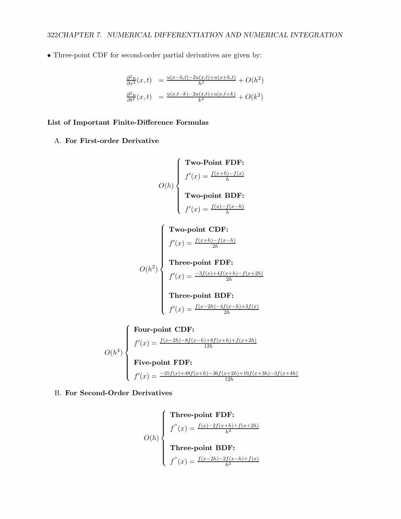
322CHAPTER 7. NUMERICAL DIFFERENTIATION AND NUMERICAL INTEGRATION
• Three-point CDF for second-order partial derivatives are given by:
∂2u∂x2 (x, t) = u(x−h,t)−2u(x,t)+u(x+h,t)
h2 +O(h2)
∂2u∂t2 (x, t) = u(x,t−k)−2u(x,t)+u(x,t+k)
k2 +O(k2)
List of Important Finite-Difference Formulas
A. For First-order Derivative
O(h)
Two-Point FDF:
f ′(x) = f(x+h)−f(x)h
Two-point BDF:
f ′(x) = f(x)−f(x−h)h
O(h2)
Two-point CDF:
f ′(x) = f(x+h)−f(x−h)2h
Three-point FDF:
f ′(x) = −3f(x)+4f(x+h)−f(x+2h)2h
Three-point BDF:
f ′(x) = f(x−2h)−4f(x−h)+3f(x)2h
O(h4)
Four-point CDF:
f ′(x) = f(x−2h)−8f(x−h)+8f(x+h)+f(x+2h)12h
Five-point FDF:
f ′(x) = −25f(x)+48f(x+h)−36f(x+2h)+16f(x+3h)−3f(x+4h)12h
B. For Second-Order Derivatives
O(h)
Three-point FDF:
f′′
(x) = f(x)−2f(x+h)+f(x+2h)h2
Three-point BDF:
f′′
(x) = f(x−2h)−2f(x−h)+f(x)h2
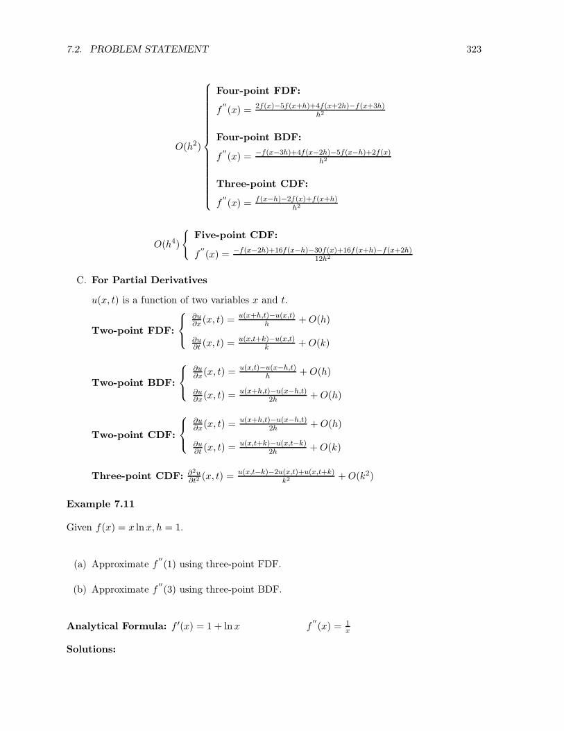
7.2. PROBLEM STATEMENT 323
O(h2)
Four-point FDF:
f′′
(x) = 2f(x)−5f(x+h)+4f(x+2h)−f(x+3h)h2
Four-point BDF:
f′′
(x) = −f(x−3h)+4f(x−2h)−5f(x−h)+2f(x)h2
Three-point CDF:
f′′
(x) = f(x−h)−2f(x)+f(x+h)h2
O(h4)
{Five-point CDF:
f′′
(x) = −f(x−2h)+16f(x−h)−30f(x)+16f(x+h)−f(x+2h)12h2
C. For Partial Derivatives
u(x, t) is a function of two variables x and t.
Two-point FDF:
∂u∂x(x, t) =
u(x+h,t)−u(x,t)h +O(h)
∂u∂t (x, t) =
u(x,t+k)−u(x,t)k +O(k)
Two-point BDF:
∂u∂x(x, t) =
u(x,t)−u(x−h,t)h +O(h)
∂u∂x(x, t) =
u(x+h,t)−u(x−h,t)2h +O(h)
Two-point CDF:
∂u∂x(x, t) =
u(x+h,t)−u(x−h,t)2h +O(h)
∂u∂t (x, t) =
u(x,t+k)−u(x,t−k)2h +O(k)
Three-point CDF: ∂2u∂t2
(x, t) = u(x,t−k)−2u(x,t)+u(x,t+k)k2
+O(k2)
Example 7.11
Given f(x) = x lnx, h = 1.
(a) Approximate f′′
(1) using three-point FDF.
(b) Approximate f′′
(3) using three-point BDF.
Analytical Formula: f ′(x) = 1 + lnx f′′
(x) = 1x
Solutions:
324CHAPTER 7. NUMERICAL DIFFERENTIATION AND NUMERICAL INTEGRATION
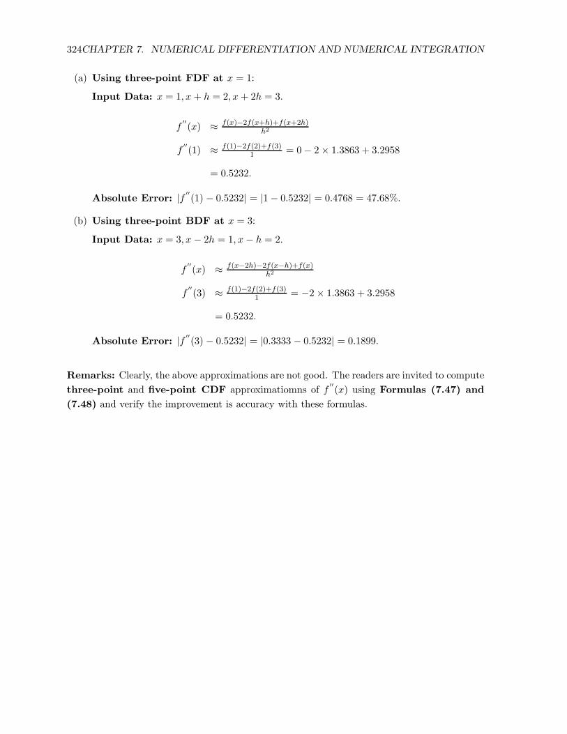
(a) Using three-point FDF at x = 1:
Input Data: x = 1, x+ h = 2, x+ 2h = 3.
f′′
(x) ≈ f(x)−2f(x+h)+f(x+2h)h2
f′′
(1) ≈ f(1)−2f(2)+f(3)1 = 0− 2× 1.3863 + 3.2958
= 0.5232.
Absolute Error: |f ′′
(1) − 0.5232| = |1− 0.5232| = 0.4768 = 47.68%.
(b) Using three-point BDF at x = 3:
Input Data: x = 3, x− 2h = 1, x− h = 2.
f′′
(x) ≈ f(x−2h)−2f(x−h)+f(x)h2
f′′
(3) ≈ f(1)−2f(2)+f(3)1 = −2× 1.3863 + 3.2958
= 0.5232.
Absolute Error: |f ′′
(3) − 0.5232| = |0.3333 − 0.5232| = 0.1899.
Remarks: Clearly, the above approximations are not good. The readers are invited to compute
three-point and five-point CDF approximatiomns of f′′
(x) using Formulas (7.47) and
(7.48) and verify the improvement is accuracy with these formulas.

7.2. PROBLEM STATEMENT 325
Exercises on Part I
7.1. (Computational) Given the following table of functional values:
x f(x) = sinx f(x) = cos x f(x) = xex
0 0 1 0
0.5 0.4794 0.8776 0.8249
1 0.8415 0.5403 2.7183
1.5 0.9975 0.0707 6.7225
2 0.9093 −0.4161 14.7781
2.5 0.5985 −0.811 30.4562
3 0.1411 −0.9900 60.2566
For each function, approximate the following derivative values and compare them with
actual values.
(a) f ′(1.8) using an interpolating polynomial approximation,
(b) f ′(0.5) using three-point FDF,
(c) f ′(1.5) using three-point CDF,
(d) f ′(2.5) using three-point BDF.
7.2. (Computational) Given the following tables of functional values for the functions (as
indicated):
(a)
x f(x) =√x sinx
0 0π4 0.6267π2 1.25333π4 1.0856
π 0
(b)
x f(x) = sin(sin(sin(x)))
0 0π4 0.6049π2 0.74563π4 0.6049
π 0
326CHAPTER 7. NUMERICAL DIFFERENTIATION AND NUMERICAL INTEGRATION
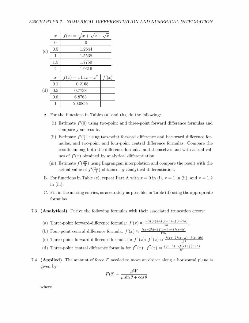
(c)
x f(x) =
√
x+√
x+√x
0 0
0.5 1.2644
1 1.5538
1.5 1.7750
2 1.9616
(d)
x f(x) = x lnx+ x2 f ′(x)
0.1 −0.2168
0.5 0.7738
0.8 6.8763
1 20.0855
A. For the functions in Tables (a) and (b), do the following:
(i) Estimate f ′(0) using two-point and three-point forward difference formulas and
compare your results.
(ii) Estimate f ′(π2 ) using two-point forward difference and backward difference for-
mulas; and two-point and four-point central difference formulas. Compare the
results among both the difference formulas and themselves and with actual val-
ues of f ′(x) obtained by analytical differentiation.
(iii) Estimate f ′(2π3 ) using Lagrangian interpolation and compare the result with the
actual value of f ′(2π3 ) obtained by analytical differentiation.
B. For functions in Table (c), repeat Part A with x = 0 in (i), x = 1 in (ii), and x = 1.2
in (iii).
C. Fill in the missing entries, as accurately as possible, in Table (d) using the appropriate
formulas.
7.3. (Analytical) Derive the following formulas with their associated truncation errors:
(a) Three-point forward-difference formula: f ′(x) ≈ −3f(x)+4f(x+h)−f(x+2h)2h .
(b) Four-point central difference formula: f ′(x) ≈ f(x−2h)−8f(x−h)+8f(x+h)12h
(c) Three-point forward difference formula for f′′
(x): f′′
(x) ≈ f(x)−2f(x+h)+f(x+2h)h2
(d) Three-point central difference formula for f′′
(x): f′′
(x) ≈ f(x−h)−2f(x)+f(x+h)h2
7.4. (Applied) The amount of force F needed to move an object along a horizontal plane is
given by
F (θ) =µW
µ sin θ + cos θ
where
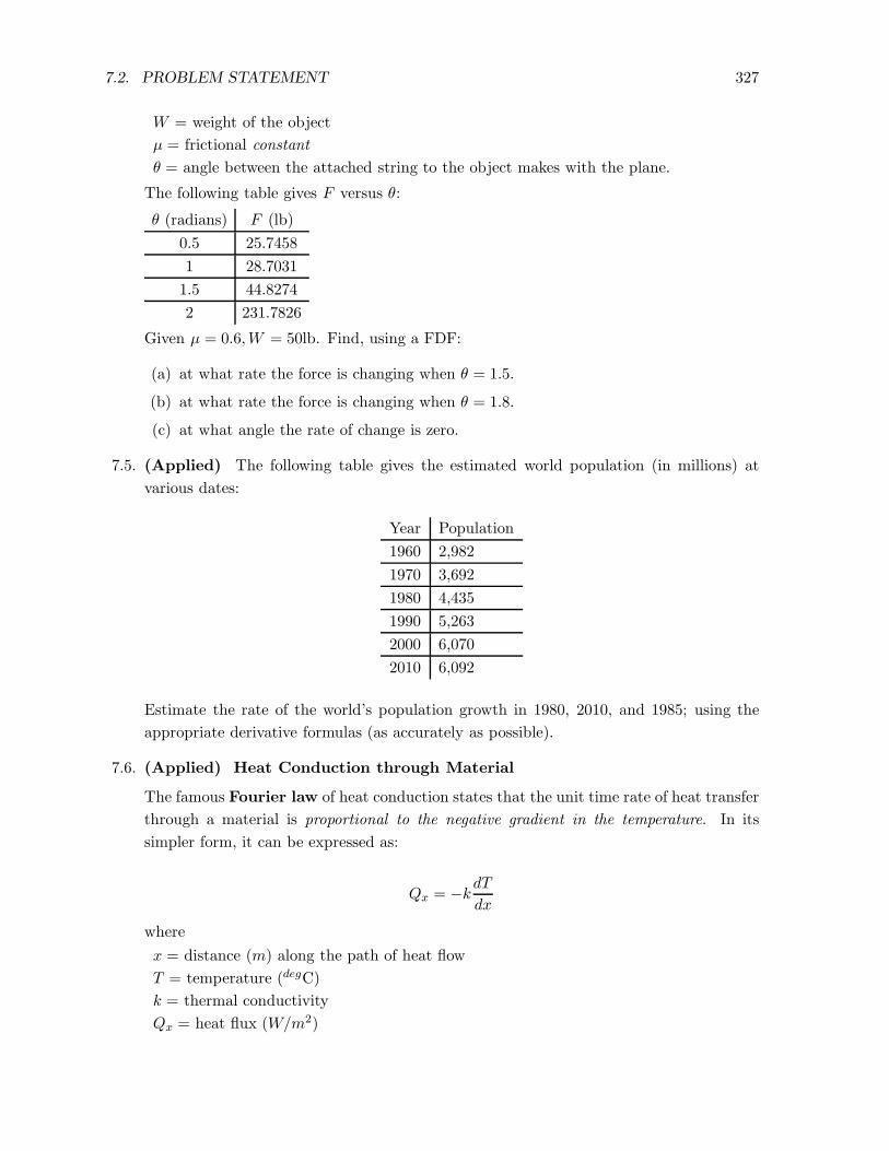
7.2. PROBLEM STATEMENT 327
W = weight of the object
µ = frictional constant
θ = angle between the attached string to the object makes with the plane.
The following table gives F versus θ:
θ (radians) F (lb)
0.5 25.7458
1 28.7031
1.5 44.8274
2 231.7826
Given µ = 0.6,W = 50lb. Find, using a FDF:
(a) at what rate the force is changing when θ = 1.5.
(b) at what rate the force is changing when θ = 1.8.
(c) at what angle the rate of change is zero.
7.5. (Applied) The following table gives the estimated world population (in millions) at
various dates:
Year Population
1960 2,982
1970 3,692
1980 4,435
1990 5,263
2000 6,070
2010 6,092
Estimate the rate of the world’s population growth in 1980, 2010, and 1985; using the
appropriate derivative formulas (as accurately as possible).
7.6. (Applied) Heat Conduction through Material
The famous Fourier law of heat conduction states that the unit time rate of heat transfer
through a material is proportional to the negative gradient in the temperature. In its
simpler form, it can be expressed as:
Qx = −kdTdx
where
x = distance (m) along the path of heat flow
T = temperature (degC)
k = thermal conductivity
Qx = heat flux (W/m2)
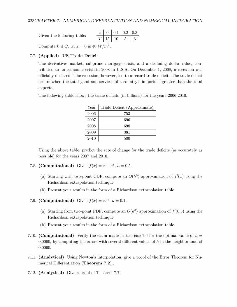
328CHAPTER 7. NUMERICAL DIFFERENTIATION AND NUMERICAL INTEGRATION
Given the following table:x 0 0.1 0.2 0.3
T 15 10 5 3
Compute k if Qx at x = 0 is 40 W/m2.
7.7. (Applied) US Trade Deficit
The derivatives market, subprime mortgage crisis, and a declining dollar value, con-
tributed to an economic crisis in 2008 in U.S.A. On December 1, 2008, a recession was
officially declared. The recession, however, led to a record trade deficit. The trade deficit
occurs when the total good and services of a country’s imports is greater than the total
exports.
The following table shows the trade deficits (in billions) for the years 2006-2010.
Year Trade Deficit (Approximate)
2006 753
2007 696
2008 698
2009 381
2010 500
Using the above table, predict the rate of change for the trade deficits (as accurately as
possible) for the years 2007 and 2010.
7.8. (Computational) Given f(x) = x+ ex, h = 0.5.
(a) Starting with two-point CDF, compute an O(h6) approximation of f ′(x) using the
Richardson extrapolation technique.
(b) Present your results in the form of a Richardson extrapolation table.
7.9. (Computational) Given f(x) = xex, h = 0.1.
(a) Starting from two-point FDF, compute an O(h3) approximation of f ′(0.5) using the
Richardson extrapolation technique.
(b) Present your results in the form of a Richardson extrapolation table.
7.10. (Computational) Verify the claim made in Exercise 7.6 for the optimal value of h =
0.0060, by computing the errors with several different values of h in the neighborhood of
0.0060.
7.11. (Analytical) Using Newton’s interpolation, give a proof of the Error Theorem for Nu-
merical Differentiation (Theorem 7.2) .
7.12. (Analytical) Give a proof of Theorem 7.7.

7.2. PROBLEM STATEMENT 329
7.13. For the functions in Exercise 7.1 and 7.2 (a), Find an optimal value of h for which the
error in computing a two-point CDF approximation to f ′(x) will be as small as possible.
MORE TO COME

330CHAPTER 7. NUMERICAL DIFFERENTIATION AND NUMERICAL INTEGRATION
3/1/13 EC
PART II. Numerical Integration
What’s Ahead
• A Case Study of Numerical Integration: Blood Flow and Cardiac Input
• Basic Quadrature Rules: Trapezoidal, Simpson, Simpson’s 38th, Corrected Trapezoidal
• Composite Rules (via Monimial and Lagrange Interpolation)
• Romberg Integration
• Gaussian Quadrature
• Improper Integral
• Multiple Integrals
• MATLAB Functions and Their Uses

7.3. STATEMENT AND SOMEAPPLICATIONS OF THE NUMERICAL INTEGRATION PROBLEM331
7.3 Statement and some Applications of the Numerical Inte-
gration Problem
In a beginning calculus course, the students learn various analytical techniques for finding the
integral∫ b
af(x) dx
and a variety of applications in science and engineering. A few of these applications include
• Finding the area between two curves y = f1(x) and y = f2(x) and the lines x = a and
x = b:
Area =
∫ b
af(x) dx, where
f(x) = f1(x)− f2(x), f1(x) ≥ f2(x),
and both functions f1(x) and f2(x) are continuous on [a, b].
• Volume of a solid obtained by rotating a curve or a region bounded by two curves about
a line
• The arc length of a function f(x) given by a(x) =∫ ba
√
1 + [f ′(x)]2 dx
• The area of a surface of revolution: the area of the surface obtained by rotating the
curve y = f(x), a ≤ x ≤ b about the x-axis is S =∫ ba 2πf(x)
√
1 + [f ′(x)]2 dx
• The center of mass or the centroid of a region at (x, y):
x =1
A
∫ b
ax f(x) dx
y =1
A
∫ b
a
1
2[f(x)]2 dx
where A is the area.
• Statistical applications, such as computing the mean of any probability density func-
tion f(x):
µ =
∫ s
−sx f(x) dx
Of particular interest is the probability density function of the normal distribution:
f(x) =1
σ√2πe−(x−µ)2/2a2
where σ =standard deviation
332CHAPTER 7. NUMERICAL DIFFERENTIATION AND NUMERICAL INTEGRATION
• Biological applications, such as the volume of the blood flow in the heart and the
cardiac output when dye is injected.
For some detailed discussions of some of these applications and many others, the readers may
refer to the authoritative calculus book by Stewart [].
Why Numerical Integration?
As in the case of numerical differentiation, the need to numerically evaluate an integral comes
from the fact that
• In many practical applications, the integrand is not explicitly known−all that’s known
are the certain discrete values of the integrand from experimental measurements.
or
• The integral is difficult to compute analytically.
We will learn various techniques of numerical integration in this Chapter.
We conclude this section with a biological application of integrals.
A Biological Application: Blood Flow and Cardiac Input
Blood Flow: Recall in Section 7.1.1, we considered the velocity of blood flow in a tube
using the law of laminar flow:
v(r) =1
4η
∆P
l(R2 − r2).
Here we consider the volume of blood flow. It can be shown (see Stewart []) that the volume V ,
of the blood that passes a cross section per unit time is given by
V =
∫ R
02πr
∆P
4ηl(R2 − x2) dx
Thus, V is a function of r. If the integrand is explicitly known, then it is quite easy to compute
this integral. However, in many practical applications, only certain discrete values of r will be
known in [0, R]. The integration thus needs to be computed numerically. We will later consider
this application with numerical data.
7.4. NUMERICAL INTEGRATION TECHNIQUES: GENERAL IDEA 333
Cardiac output: The cardiac output of the heart is the volume of blood pumped by the
heart per unit time. Usually, a dye is injected into the right atrium to measure the cardiac
output.
Let c(t) denote the concentration of the dye at time t and let the dye be injected for the time
interval [0, T ]. Then the cardiac output CO is given by:
CO =A
∫ T0 c(t) dt
where A is the amount of dye.
Again, in practical applications, c(t) will be measured at certain equally spaced times over the
interval [0, T ]. Thus, all will be known to a user is some discrete values of c(t) at these instants
of time, from where the integral must be computed numerically.
A solution of this problem with numerical data will be considered later in this Chapter.
Numerical Integration Problem
Given
(i) the functional values f0, f1, . . . , fn, of a function f(x), at x0, x1, . . . , xn, where a = x0 <
x1 < x2 . . . < xn−1 < xn = b,
or
(ii) an integratable function f(x) itself over [a, b].
Compute: an approximate value of I =
∫ b
af(x)dx using these functional values or those
computed from the given function.
7.4 Numerical Integration Techniques: General Idea
The numerical techniques discussed in this chapter have the following form:∫ b
af(x)dx ≈ I = w0f(x0) + w1f(x1) + · · ·+ wnf(xn) = w0f0 + w1f1 + · · ·+ wnfn
where x0, x1, . . . , xn are called the nodes, and w0, w1, . . . , wn are called the weights. Thus,
we can have two types of formulas:
334CHAPTER 7. NUMERICAL DIFFERENTIATION AND NUMERICAL INTEGRATION
Type 1. The (n+1) nodes are given and the (n+1) weights are determined by the rule. The
well-known classical quadrature rules, such as the Trapezoidal rule and Simpson’s rule are
examples of this type.
Type 2. Both nodes and weights are determined by the rule. Gaussian quadrature is an
example of this type.
We will discuss Type 1 first.
General Idea. The polynomial functions are easier to integrate. Thus, to evaluate
∫ b
af(x)
numerically, the obvious things to do are:
• Find the interpolating polynomial Pn(x) of degree at most n, passing through the (n + 1)
points: (x0, f0), (x1, f1), . . . , (xn, fn).
• Evaluate I =
∫ b
aPn(x)dx and accept this value as an approximation to I.
Exactness of the Type 1 Quadrature Rules: These rules, by construction, should be exact
for all polynomials of degree less than or equal to n.
We know that there are different ways to construct the unique interpolating polynomial using
different basis functions.
We will describe here the quadrature rules based onmonomial and Lagrange interpolations.
7.5 Numerical Integration Techniques Based on Monomial In-
terpolation
A numerical quadrature formula based on monomial basis interpolation, by definition, is exact
for the basis polynomials {1, x, x2, . . . , xn}. This observation leads to a system of (n + 1)
equations in (n+ 1) unknowns, w0, w1, . . . , wn, as shown below.
7.5. NUMERICAL INTEGRATION TECHNIQUES BASEDONMONOMIAL INTERPOLATION335
f(x) = 1 :
∫ b
a1dx = w0 + w1 + · · ·+ wn
=⇒ b− a = w0 + w1 + · · ·+ wn
f(x) = x :
∫ b
axdx = w0x0 + w1x1 + w2x2 + · · ·+ wnxn
=⇒ b2−a2
2 = w0x0 + w1x1 + · · ·+ wnxn
...
f(x) = xn :
∫ b
axndx = w0x
n0 + w1x
n1 + · · ·+ wnx
nn
=⇒ bn+1−an+1
n+1 = w0xn0 + w1x
n1 + · · ·+ wnx
nn
The above (n + 1) equations are assembled as:
w0 + w1 + · · ·+ wn = b− a
w0x0 + w1x1 + · · ·+ wnxn = b2−a2
2
...
w0xn0 + w1x
n1 + · · ·+ wnx
nn = bn+1−an+1
n+1
In matrix-vector notations:
1 1 · · · 1
x0 x1 · · · xn...
. . ....
xn−10 xn−1
n · · · xn−1n
xn0 xn1 · · · xnn
w0
w1
...
wn−1
wn
=
b− ab2−a2
2...
bn−an
nbn+1−an+1
n+1
The readers will recognize that the matrix on the left-hand side is a Vandermonde matrix,
which is nonsingular by virtue of the fact that x0, x1, . . . , xn are distinct. The unique
solution of this system will yield the unknowns w0, w1, . . . , wn.
Uniqueness. Thus, we have the following uniqueness result:
Given x0 < x1 < x2 . . . < xn, there exist an unique set of weights w0, w1, . . . , wn such that
∫ b
af(x)dx ≈ w0f0 + w1f1 + · · ·+ wnfn
where fi = f(xi), i = 0, 1, . . . , n.
336CHAPTER 7. NUMERICAL DIFFERENTIATION AND NUMERICAL INTEGRATION
The above process is sometimes called the method of undetermined coefficients.
Special cases. The following two special cases give rise to two famous quadrature rules.
n = 1 → Trapezoidal rule (x0 = a, x1 = b)∫ b
af(x)dx ≈ b− a
2[f(a) + f(b)]
n = 2 → Simpson’s rule (x0 = a, x1 = a+b2 , x2 = b)
∫ b
af(x)dx ≈ b− a
6[f(a) + 4f(
a+ b
2) + f(b)]
7.6 Numerical Integration Rules Based on Lagrange Interpola-
tion
We will now derive Trapezoidal, Simpson’s, and other rules based on Lagrange interpolation.
The use of Lagrange interpolation also will help us derive the error formulas for these rules.
The Idea is as follows:
• Given n, find the Lagrange interpolating polynomial Pn(x) of degree at most n, approxi-
mating f(x):
Pn(x) = f0L0(x) + f1L1(x) + · · ·+ fnLn(x)
where L0(x), L1(x), . . . , Ln(x) are Lagrange polynomials each of degree n.
• Compute
∫ b
aPn(x)dx and accept the result as an approximation to
∫ b
af(x)dx.
7.6.1 Trapezoidal Rule
f(x) ≈ Lagrange Interpolating polynomial of degree 1 =⇒ Trapezoidal Rule
In this case, there are only two nodes: x0, x1.
7.6. NUMERICAL INTEGRATION RULES BASEDON LAGRANGE INTERPOLATION337
X Xx0 = a x1 = b
The Lagrange interpolating polynomial P1(x) of degree 1 is:
P1(x) = L0(x)f0 + L1(x)f1.
So, I =
∫ b=x1
a=x0
f(x)dx ≈∫ x1
x0
[L0(x)f0 + L1(x)f1]dx.
Recall that L0(x) =x− x1x0 − x1
, and L1(x) =x− x0x1 − x0
.
Thus, IT = trapezoidal rule approximation of I is given by
IT =
∫ x1
x0
[x− x1x0 − x1
f0 +x− x0x1 − x0
f1
]
dx
=f0
x0 − x1
∫ x1
x0
(x− x1)dx+f1
x1 − x0
∫ x1
x0
(x− x0)dx
=f0
x0 − x1
[(x− x1)
2
2
]x1
x0
+f1
x1 − x0
[(x− x0)
2
2
]x1
x0
=(x1 − x0)
2(f0 + f1).
Let x1 − x0 = h. Since f0 = f(x0) = f(a), and f1 = f(x1) = f(a), we obtain
Trapezoidal Rule
IT =(x1 − x0)
2(f0 + f1) =
h
2(f0 + f1) =
b− a
2(f(a) + f(b)) (7.49)
Error in Trapezoidal Rule
Since the above formula only gives a crude approximation to the actual value of the integral,
we need to assess the error.
To obtain an error formula for this integral approximation, recall that the error formula for
interpolation with a polynomial of degree at most n is given by
En(x) =f (n+1)(ξ(x))Ψn(x)
(n+ 1)!, (7.50)

338CHAPTER 7. NUMERICAL DIFFERENTIATION AND NUMERICAL INTEGRATION
where Ψn(x) = (x− x0)(x− x1) . . . (x− xn), and a ≤ ξ ≤ b (a ≡ x0, b ≡ xn).
Since in case of the Trapezoidal rule, n = 1, the error associated interpolation error is:
E1(x) =f
′′
(ξ(x))Ψ1(x)
2!,
where Ψ1(x) = (x− x0)(x− x1), and f′′
(x) is the second derivative of f(x).
Integrating this formula we have the following error formula for the Trapezoidal rule
(denoted by ET (x)):
ET (x) =
∫ x1
x0
f′′
(ξ(x))
2!(x− x0)(x− x1)dx =
∫ x1
x0
f′′
(ξ(x))
2!Ψ1(x). (7.51)
We now show how the above formula can be simplified. TheWeighted Mean Value Theorem
(WMT) from calculus will be needed for this purpose.
Weighted Mean Value Theorem for Integrals (WMT)
Let
(i) f(x) be continuous on [a, b]
(ii) g(x) does not change sign on [a, b]
Then there exists a number c in (a, b) such that
∫ b
af(x)g(x)dx = f(c)
∫ b
ag(x)dx
To apply the WMT to (7.51), we note that
(i) f′′
(x) is continuous on [x0, x1] (Hypothesis (i) of WMT is satisfied).
(ii) Ψ1(x) = (x − x0)(x − x1) does not change sign over [x0, x1]. This is because for any x
in [x0, x1], (x− x0) > 0 and (x− x1) < 0 (Hypothesis (ii) of WMT is satisfied).
So, by applying the WMT to ET (x), with g(x) = Ψ(x) and noting that h = x1 − x0, we obtain
7.6. NUMERICAL INTEGRATION RULES BASEDON LAGRANGE INTERPOLATION339
Error in the Trapezoidal Rule
ET =f
′′
(η)
2!
∫ x1
x0
(x− x0)(x− x1)dx =−h312
f ′′(η)
= −(b−a)3
12 f′′
(η) = −(b−a)12 h2f
′′
(η)
(7.52)
where a < η < b.
Trapezoidal Rule with Error Formula
∫ x1=b
x0=af(x)dx =
b− a
2[f(a) + f(b)]
︸ ︷︷ ︸
Trapezoidal Rule
− b− a
12h2f
′′
(η)︸ ︷︷ ︸
Error
, a < η < b.
Exactness of Trapezoidal Rule: From the above error formula it follows that the Trapezoidal
rule is exact only for polynomials of degree 1 or less. This is because, for all these polynomials,
f′′
(x) = 0, and is non zero, whenever f(x) is of degree 2 and higher.
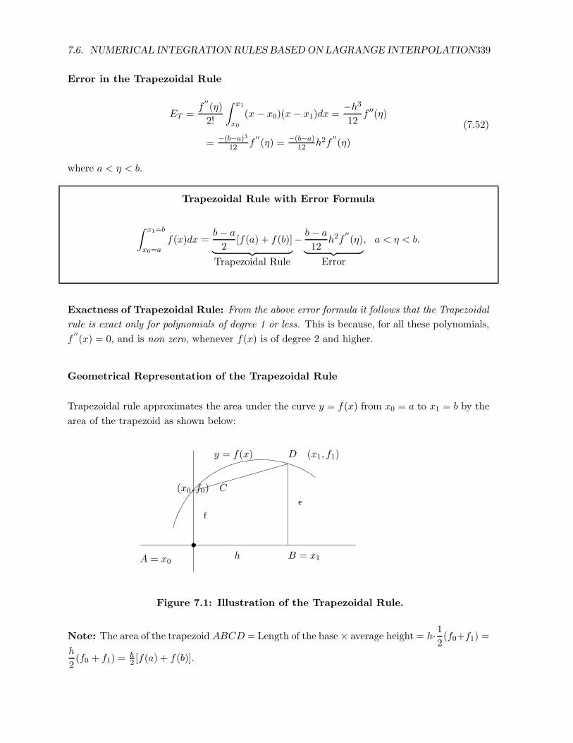
Geometrical Representation of the Trapezoidal Rule
Trapezoidal rule approximates the area under the curve y = f(x) from x0 = a to x1 = b by the
area of the trapezoid as shown below:
e
f
A = x0 B = x1
(x0, f0) C
y = f(x)
h
D (x1, f1)
Figure 7.1: Illustration of the Trapezoidal Rule.
Note: The area of the trapezoid ABCD = Length of the base× average height = h·12(f0+f1) =
h
2(f0 + f1) =
h2 [f(a) + f(b)].
340CHAPTER 7. NUMERICAL DIFFERENTIATION AND NUMERICAL INTEGRATION
7.6.2 Simpson’s Rule
If f(x) is approximated by Lagrange interpolating polynomial of degree 2 and the integration
is taken over [a, b] with the interpolating polynomial as the integrand, the result is Simpson’s
rule.
f(x) ≈ Lagrange Interpolating polynomial of degree 2 =⇒ Simpson’s Rule
The three points of interpolation in this case are: x0, x1, and x2.
x0 = a x1 x2 = b
The Lagrange interpolating polynomial P2(x) = L0(x)f0 + L1(x)f1 + L2(x)f2.
So,
I =
∫ b=x2
a=x0
f(x)dx ≈∫ x2
x0
[L0(x)f0 + L1(x)f1 + L2(x)f2]dx (7.53)
Now, L0(x) =(x− x1)(x− x2)
(x0 − x1)(x0 − x2), L1(x) =
(x− x0)(x− x2)
(x1 − x0)(x1 − x2),
and L2(x) =(x− x0)(x− x1)
(x2 − x0)(x2 − x1).
Let h be the distance between two consecutive points of interpolation, assumed to be equally
spaced. That is, x1 − x0 = h and x2 − x1 = h.
Substituting these expressions of L0(x), L1(x) and L2(x) into (7.53) and integrating, we obtain
[Exercise] the famous Simpson’s Rule:
IS =h
3(f0 + 4f1 + f2) (7.54)
Noting that
h = b−a2
f0 = f(x0) = f(a)
f1 = f(x1) = f(x0 + h) = f(a+ b−a2 ) = f(a+b
2 )
f2 = f(x2) = f(b)
We can rewrite (7.54) as:∫ b
af(x)dx ≈ IS =
b− a
6
[
f(a) + 4f
(a+ b
2
)
+ f(b)
]
.

7.6. NUMERICAL INTEGRATION RULES BASEDON LAGRANGE INTERPOLATION341
Error in Simpson’s Rule
Since n = 2, the error formula (7.50) becomes
E2(x) = 13!f
3(ξ(x))Ψ2(x)dx,
where Ψ2(x) = (x− x0)(x− x1)(x− x2)
Since Ψ2(x) does change sign in [x0, x2], we can not apply WMT directly to obtain the error
formula for Simpson’s rule. In this case, we use the following modified formula:
Modified Integration Error Formula
Let
(i) Ψn(x) = (x− x0)(x− x1) · · · (x− xn) be such that it changes sign on (a, b), but
∫ b
aΨn(x)dx = 0
(ii) xn+1 be a point such that Ψn+1(x) = (x− xn+1)Ψn(x) is of one sign in [a, b].
(iii) f(x) is (n+ 2) times continuously differentiable,
then application of the MVT for integration yields:
En+1(x) =1
(n+ 2)!f (n+2)(η)
∫ b
aΨn+1(x)dx (7.55)
where a < η < b.
To apply the above modified error formula to obtain an error expression for Simpson’s rule, we
note the following:
(i)
∫ x2
x0
Ψ2(x)dx =
∫ x2
x0
(x− x0)(x− x1)(x− x2)dx = 0 (Hypothesis (i) is satisfied).
(ii) If a point x3 is chosen as x3 ≡ x1, then
Ψ3(x) = (x− x3)Ψ2(x) = (x− x1)(x− x0)(x− x1)(x− x2) = (x− x1)2(x− x0)(x− x2).
is of the same sign in [x0, x3] (Hypothesis (ii) is satisfied).
342CHAPTER 7. NUMERICAL DIFFERENTIATION AND NUMERICAL INTEGRATION
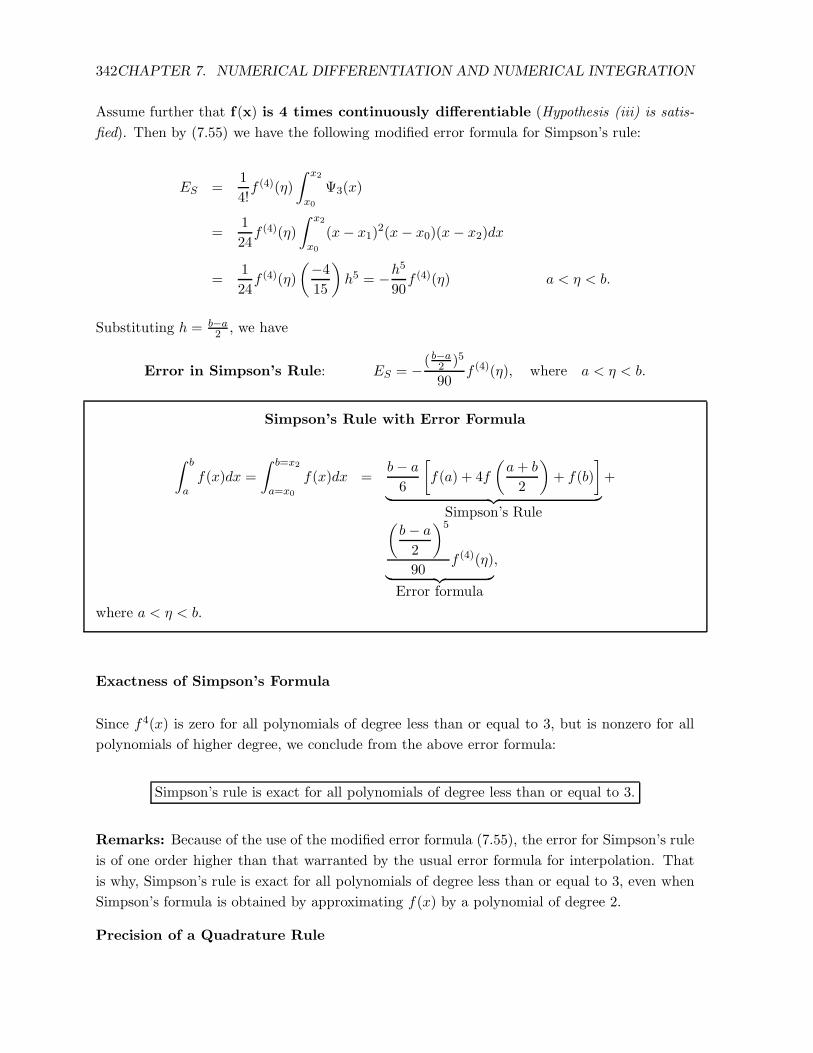
Assume further that f(x) is 4 times continuously differentiable (Hypothesis (iii) is satis-
fied). Then by (7.55) we have the following modified error formula for Simpson’s rule:
ES =1
4!f (4)(η)
∫ x2
x0
Ψ3(x)
=1
24f (4)(η)
∫ x2
x0
(x− x1)2(x− x0)(x− x2)dx
=1
24f (4)(η)
(−4
15
)
h5 = −h5
90f (4)(η) a < η < b.
Substituting h = b−a2 , we have
Error in Simpson’s Rule: ES = −( b−a2 )5
90f (4)(η), where a < η < b.
Simpson’s Rule with Error Formula
∫ b
af(x)dx =
∫ b=x2
a=x0
f(x)dx =b− a
6
[
f(a) + 4f
(a+ b
2
)
+ f(b)
]
︸ ︷︷ ︸
Simpson’s Rule
+
(b− a
2
)5
90f (4)(η)
︸ ︷︷ ︸
Error formula
,
where a < η < b.
Exactness of Simpson’s Formula
Since f4(x) is zero for all polynomials of degree less than or equal to 3, but is nonzero for all
polynomials of higher degree, we conclude from the above error formula:
Simpson’s rule is exact for all polynomials of degree less than or equal to 3.
Remarks: Because of the use of the modified error formula (7.55), the error for Simpson’s rule
is of one order higher than that warranted by the usual error formula for interpolation. That
is why, Simpson’s rule is exact for all polynomials of degree less than or equal to 3, even when
Simpson’s formula is obtained by approximating f(x) by a polynomial of degree 2.
Precision of a Quadrature Rule
7.6. NUMERICAL INTEGRATION RULES BASEDON LAGRANGE INTERPOLATION343
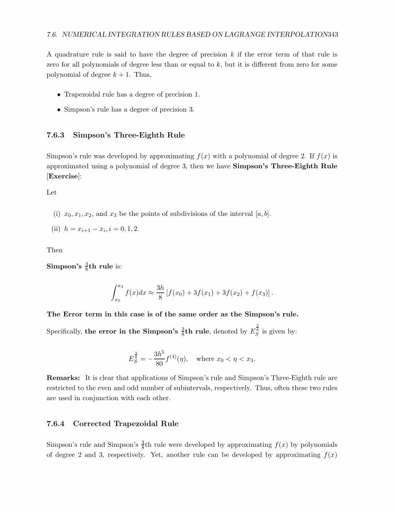
A quadrature rule is said to have the degree of precision k if the error term of that rule is
zero for all polynomials of degree less than or equal to k, but it is different from zero for some
polynomial of degree k + 1. Thus,
• Trapezoidal rule has a degree of precision 1.
• Simpson’s rule has a degree of precision 3.
7.6.3 Simpson’s Three-Eighth Rule
Simpson’s rule was developed by approximating f(x) with a polynomial of degree 2. If f(x) is
approximated using a polynomial of degree 3, then we have Simpson’s Three-Eighth Rule
[Exercise]:
Let
(i) x0, x1, x2, and x3 be the points of subdivisions of the interval [a, b].
(ii) h = xi+1 − xi, i = 0, 1, 2.
Then
Simpson’s 38th rule is:
∫ x3
x0
f(x)dx ≈ 3h
8[f(x0) + 3f(x1) + 3f(x2) + f(x3)] .
The Error term in this case is of the same order as the Simpson’s rule.
Specifically, the error in the Simpson’s 38th rule, denoted by E
3
8
S is given by:
E3
8
S = −3h5
80f (4)(η), where x0 < η < x3.
Remarks: It is clear that applications of Simpson’s rule and Simpson’s Three-Eighth rule are
restricted to the even and odd number of subintervals, respectively. Thus, often these two rules
are used in conjunction with each other.
7.6.4 Corrected Trapezoidal Rule
Simpson’s rule and Simpson’s 38th rule were developed by approximating f(x) by polynomials
of degree 2 and 3, respectively. Yet, another rule can be developed by approximating f(x)

344CHAPTER 7. NUMERICAL DIFFERENTIATION AND NUMERICAL INTEGRATION
by Hermite interpolating polynomial of degree 3, with a special choice of the nodes as:
x0 = x1 = a and x2 = x3 = b.
This rule, for obvious reasons, is called the corrected trapezoidal rule (ICT). This rule along
with the error expression is stated below. Their proofs are left as an [Exercise].
Corrected Trapezoidal Rule with Error Formula
∫ b
af(x)dx ≈ ITC =
b− a
2[f(a) + f(b)] +
(b− a)2
12[f ′(a)− f ′(b)]
︸ ︷︷ ︸
Corrected Trapezoidal Rule
+(b− a)5
720f (4)(η)
︸ ︷︷ ︸
Error Formula
Remarks: Comparing the error formulas of the trapezoidal rule and the corrected trapezoidal
rule, it is obvious that the corrected trapezoidal rule is much more accurate than the trapezoidal
rule.
However, the price to pay for this gain is that ICT requires computations of f ′(a) and f ′(b).
Example 7.12 (a) Approximate
∫ 1
0cos xdx using
(i) Trapezoidal rule
(ii) Simpson’s rule
(iii) Simpson’s 38 th rule
(iv) Corrected trapezoidal rule
(b) In each case, compute the maximum error and compare this maximum error with the
actual error, obtained by an analytical formula.
Solution (a).
(i) Trapezoidal Rule Approximation
Input Data: x0 = a = 0, x1 = b = 1, f(x) = cos x
Formula to be used: IT = b−a2 [f(a) + f(b)]
IT = 12 [cos(0) + cos(1)] = 1
2(1 + 0.5403) = 0.7702.
(ii) Simpson’s Rule Approximation
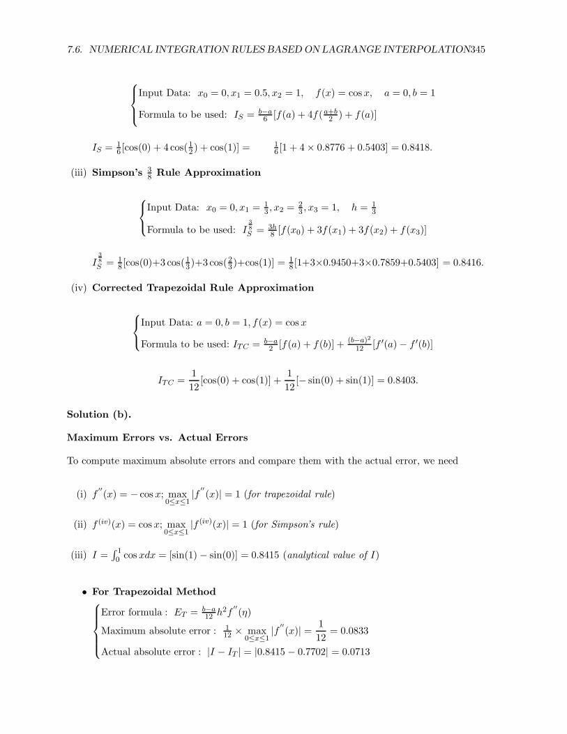
7.6. NUMERICAL INTEGRATION RULES BASEDON LAGRANGE INTERPOLATION345
Input Data: x0 = 0, x1 = 0.5, x2 = 1, f(x) = cosx, a = 0, b = 1
Formula to be used: IS = b−a6 [f(a) + 4f(a+b
2 ) + f(a)]
IS = 16 [cos(0) + 4 cos(12 ) + cos(1)] = 1
6 [1 + 4× 0.8776 + 0.5403] = 0.8418.
(iii) Simpson’s 38 Rule Approximation
Input Data: x0 = 0, x1 = 13 , x2 =
23 , x3 = 1, h = 1
3
Formula to be used: I3
8
S = 3h8 [f(x0) + 3f(x1) + 3f(x2) + f(x3)]
I3
8
S = 18 [cos(0)+3 cos(13)+3 cos(23)+cos(1)] = 1
8 [1+3×0.9450+3×0.7859+0.5403] = 0.8416.
(iv) Corrected Trapezoidal Rule Approximation
Input Data: a = 0, b = 1, f(x) = cos x
Formula to be used: ITC = b−a2 [f(a) + f(b)] + (b−a)2
12 [f ′(a)− f ′(b)]
ITC =1
12[cos(0) + cos(1)] +
1
12[− sin(0) + sin(1)] = 0.8403.
Solution (b).
Maximum Errors vs. Actual Errors
To compute maximum absolute errors and compare them with the actual error, we need
(i) f′′
(x) = − cos x; max0≤x≤1
|f ′′
(x)| = 1 (for trapezoidal rule)
(ii) f (iv)(x) = cos x; max0≤x≤1
|f (iv)(x)| = 1 (for Simpson’s rule)
(iii) I =∫ 10 cos xdx = [sin(1)− sin(0)] = 0.8415 (analytical value of I)
• For Trapezoidal Method
Error formula : ET = b−a12 h
2f′′
(η)
Maximum absolute error : 112 × max
0≤x≤1|f ′′
(x)| = 1
12= 0.0833
Actual absolute error : |I − IT | = |0.8415 − 0.7702| = 0.0713

346CHAPTER 7. NUMERICAL DIFFERENTIATION AND NUMERICAL INTEGRATION
• For Simpson’s Method
Error formula : ES = − ( b−a
2)5
90 f (iv)(η)
Maximum absolute error : 132 × 1
90 max0≤x≤1
|f (4)(x)| = 1
32× 1
90= 3.477 × 10⁻⁴
Actual absolute error : |I − IS | = |0.8415 − 0.8418| = 3× 10⁻⁴
• For Corrected Trapezoidal Rule
Error formula : (b−a)5
720 f (4)(η)
Maximum absolute error : 1720 max
0≤x≤1|f (4)(x)| = 1
720= 0.0014
Actual absolute error : |I − ITC | = |0.8415 − 0.8403| = 0.0012
• For Simpson’s 38th Rule [Exercise]
Observations: (i) Actual absolute error in each case is comparable with the corresponding
maximum (worst possible) error, but is always less than the latter.
(ii) The corrected trapezoidal rule is more accurate than the trapezoidal rule.
(iii) Simpson’s rule is most accurate.
7.7 Newton-Cotes Quadrature
Trapezoidal, Simpson’s and Simpson’s Three-Eighth rules, developed in the last section are
special cases of a more general rule, known as, the Closed Newton-Cotes (CNC) rule.
An n-point closed Newton-Cotes rule over [a, b] has the (n+1) nodes: xi = a+ i(b− a)
n, i =
0, 1, · · · , n.
Thus, it is easy to see that for
• n = 1 ⇒ Trapezoidal Rule (Two nodes: x0 = a, x1 = b)
• n = 2 ⇒ Simpson’s Rule (Three nodes: x0 = a, x1 =a+ b
2, x2 = b)
• n = 3 ⇒ Simpson’s 38th Rule.
• n = 4 ⇒ Boole’s Rule [Exercise]
∫ x4
x0
f(x)dx ≈ 2h
45(7f0 + 32f1 + 12f2 + 32f3 + 7f4).

7.7. NEWTON-COTES QUADRATURE 347
(Note that CNC Rule includes the end points of the nodes.)
The open Newton-Cotes has the (n + 1) nodes which do not include the end points.
These nodes are given by: xi = a+ i(b− a)
n+ 2, i = 1, 2, · · · , n.
Mid-Point Rule: A well-known example of the n-point open Newton-Cotes rule is the mid-
point rule (with n = 0). Thus, the midpoint rule is based on interpolation of f(x)
with a constant function. The only node in this case is: x1 =a+ b
2.
So,
IM = Midpoint Approximation to the Integral
∫ b
af(x)dx = (b− a)f
(a+ b
2
)
.
Error Formula for the Midpoint Rule:
In this case Ψ0(x) = x− x1 = x− a+ b
2changes sign in (a, b).
However, note that if we let x0 = x1, then
Ψ1(x) = (x− x1)2 =
(
x− a+ b
2
)2
is always of the same sign. Thus, as in the case of Simpson’s rule, we can derive the error
formula for IM [Exercise]:
EM = f ′′(η)(b− a)3
24, where a < η < b.
Midpoint Rule with Error Formula
∫ b
af(x)dx ≈ IM = (b− a)f
(a+ b
2
)
︸ ︷︷ ︸
Midpoint Rule
+ f ′′(η)(b − a)3
24︸ ︷︷ ︸
Error Formula
, where a < η < b.
Remark: Comparing the error terms of IM and IT , we easily see that the midpoint rule is more
accurate than the trapezoidal rule. The following simple example compares the accuracy
of these different rules: trapezoidal, Simpson’s, midpoint, and corrected trapezoidal.
Example 7.13
Apply the midpoint, trapezoidal, corrected trapezoidal, and Simpson’s rule to approximate
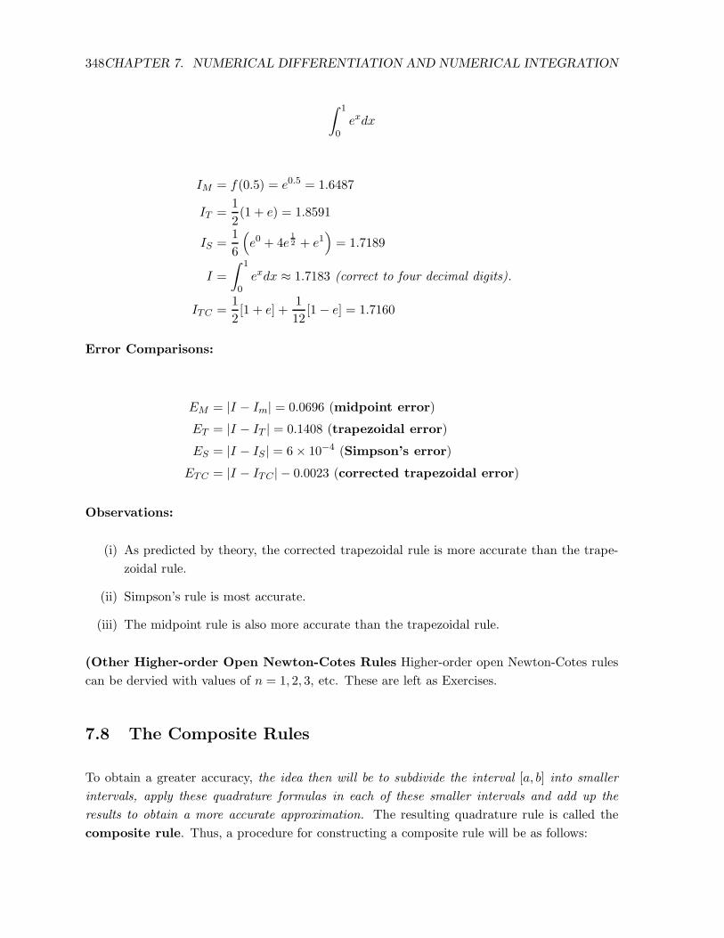
348CHAPTER 7. NUMERICAL DIFFERENTIATION AND NUMERICAL INTEGRATION
∫ 1
0exdx
IM = f(0.5) = e0.5 = 1.6487
IT =1
2(1 + e) = 1.8591
IS =1
6
(
e0 + 4e1
2 + e1)
= 1.7189
I =
∫ 1
0exdx ≈ 1.7183 (correct to four decimal digits).
ITC =1
2[1 + e] +
1
12[1− e] = 1.7160
Error Comparisons:
EM = |I − Im| = 0.0696 (midpoint error)
ET = |I − IT | = 0.1408 (trapezoidal error)
ES = |I − IS | = 6× 10⁻⁴ (Simpson’s error)
ETC = |I − ITC | − 0.0023 (corrected trapezoidal error)
Observations:
(i) As predicted by theory, the corrected trapezoidal rule is more accurate than the trape-
zoidal rule.
(ii) Simpson’s rule is most accurate.
(iii) The midpoint rule is also more accurate than the trapezoidal rule.
(Other Higher-order Open Newton-Cotes Rules Higher-order open Newton-Cotes rules
can be dervied with values of n = 1, 2, 3, etc. These are left as Exercises.
7.8 The Composite Rules
To obtain a greater accuracy, the idea then will be to subdivide the interval [a, b] into smaller
intervals, apply these quadrature formulas in each of these smaller intervals and add up the
results to obtain a more accurate approximation. The resulting quadrature rule is called the
composite rule. Thus, a procedure for constructing a composite rule will be as follows:

7.8. THE COMPOSITE RULES 349
• Divide [a, b] into n equal subintervals. Let the points of the subdivisions be:
a = x0 < x1 < x2 . . . < xn−1 < xn = b.
Assume that each of these intervals are of equal length. Let h =b− a
n= the length of
each of these subintervals.
Then x0 = a, x1 = a+ h, x2 = a+ 2h, . . . , xn = b = a+ nh.
• Apply a quadrature rule in each of these subintervals.
• Add the results.
The Composite Trapezoidal Rule
∫ b
af(x)dx =
∫ x1
x0=af(x)dx+
∫ x2
x1
f(x)dx+ . . .+
∫ xn=b
xn−1
f(x)dx
Applying the basic trapezoidal rule (7.49) to each of the integrals on the right-hand side and
adding the results, we obtain the composite trapezoidal rule, ICT .
Thus,
∫ b
af(x)dx ≈ ICT =
h
2(f0 + f1) +
h
2(f1 + f2) + . . . +
h
2(fn−1 + fn)
= h
(f02
+ f1 + f2 + . . .+ fn−1 +fn2
)
.
Noting that
f0 = f(x0) = f(a)
f1 = f(x1) = f(a+ h)...
fn−1 = f(xn−1) = f(x+ (n− 1)h)
fn = f(xn) = f(b)
We can write ICT as
ICT =h
2[f(a) + 2 (f(a+ h) + 2f(a+ 2h) + · · ·+ 2f(a+ (n− 1)h) + f(b))]
Using the summation notation, we have the following formula for the composite trapezoidal
rule:
350CHAPTER 7. NUMERICAL DIFFERENTIATION AND NUMERICAL INTEGRATION
ICT =h
2
[
f(a) + 2h−l∑
i=1
f(a+ ih) + f(b)
]
Note: n = 1 ⇒ ICT = the basic trapezoidal rule (7.65).
7.8.1 The Error Formula for Composite Trapezoidal Rule
The error formula for ICT is obtained by adding the individual error terms of the trapezoidal
rule in each of the subintervals. Thus, the error formula for the composite trapezoidal rule,
denoted by ECT , is given by:
ECT =−h312
[f ′′(η1) + f ′′(η2) + . . .+ f ′′(ηn)]
where xi−1 < ηi < xi, i = 2, 3, . . . , n.
Simplification of the Error Formula
.
To simplify the expression within the brackets, we assume that f′′
(x) is continuous on [a, b].
Then by Intermediate Value Theorem (IVT), we can write
f′′
(η1) + . . .+ f′′
(ηn) = nf′′
(η), where η1 < η < ηn.
Thus, the above formula for ECT reduces to:
ECT = −nh3
12 f′′(η), where η1 < η < ηn.
= −n (b−a)n · h2
12 f′′(η) = − (b−a)
12 h2f ′′(η),
(because h = b−a
n
).

7.8. THE COMPOSITE RULES 351
The Composite Trapezoidal Rule With Error Term
∫ b=xn
a=x0
f(x)dx =h
2
[
f(a) + 2n−1∑
i=1
f(a+ ih) + f(b)
]
︸ ︷︷ ︸
Composite Trapezoidal Rule
− b− a
12h2f ′′(η)
︸ ︷︷ ︸
Error
where a < η < b.
7.8.2 The Composite Simpson’s Rule (ICS)
Since Simpson’s rule was obtained with two subintervals, in order to derive the CSR, we divide
the interval [a, b] into even number of subintervals, say n = 2m, where m is a positive integer
and then apply Simpson’s rule in each of those subintervals and finally, add up the results.
Obtaining Composite Simpson’s Rule
• Divide the interval [a, b] into n even number of equal subintervals: [x0, x2], [x2, x4] . . . , [xn−2, xn].
Set h = b−an .
Then we have∫ b
af(x)dx =
∫ x2
x0
f(x)dx+
∫ x4
x2
f(x)dx+ · · ·+∫ x2n
xn−2
f(x)dx.
• Apply the basic Simpson’s rule (Formula 7.54) to each of the integrals on the right-hand
side and add the results to obtain the Composite Simpson’s rule, ICS .
ICS =h
3[(f0 + 4f1 + f2) + (f2 + 4f3 + f4) + . . . + (fn−2 + 4fn−1 + fn)]
=h
3[(f(a) + f(b) + 4(f1 + f3 + . . . + fn−1) + 2(f2 + f4 + . . .+ fn−2)] .
(7.56)
(Note that f0 = f(x0) = f(a) and fn = f(xn) = f(b)).
Note: n = 2 ⇒ The basic Simpson’s rule (7.54).
The Error in Composite Simpson’s Rule
The error in composite Simpson’s Rule, denoted by ESC , is given by
352CHAPTER 7. NUMERICAL DIFFERENTIATION AND NUMERICAL INTEGRATION
ESC =
−h590
[
f (iv)(η1) + f (iv)(η2) + . . .+ f (iv)(ηn
2)]
,
where x2i−2 < ηi < x2i, i = 1, . . . ,n
2.
A Simplified Expression for the Error
As before, we can now invoke IVT to simplify the above error expression. Assuming that
f (iv)(x) is continuous on [a, b], by IVT, we can write
f (iv)(η1) + f (iv)(η2) + . . .+ f (iv)(ηn) = nf (iv)(ηn
2),
where η1 < η < ηn
2.
Thus, the error formula for the composite Simpson’s rule is simplified to:
ECS =−h590
× n
2f (iv)(η)
=−h5180
(b− a)
hf (iv)(η) =
−h4180
(b− a)f (iv)(η).(
Since n =b− a
h
)
.
The Composite Simpson’s Rule with Error Term
∫ b
af(x)dx =
h
3[(f0 + fn) + 4(f1 + . . .+ fn−1) + 2(f2 + . . .+ fn−2)]−
h4
180(b− a)f (4)(η)
=h
3[f(a) + f(b) + 4(f1 + · · ·+ fn−1) + 2(f2 + · · · + fn−2]
︸ ︷︷ ︸
Composite Simpson’s Rule
− h4
180(b− a)f (4)(η)
︸ ︷︷ ︸
Error
Example 7.14
Let f(x) =
{
x if 0 ≤ x ≤ 12
1− x if 12 ≤ x ≤ 1
(a) Trapezoidal Rule over [0, 1] with h = 1
IT = 12 (f(0) + f(1)) = 1
2(0 + 0) = 0
7.8. THE COMPOSITE RULES 353
(b) Composite Trapezoidal Rule with h = 12
ICT = 14
(f(0) + f(12)
)+ 1
4
(f(12) + f(1)
)
= 14
(0 + 1
2 +12 + 0
)= 1
4(1) =14
Solution (c). Simpson’s Rule over [0, 1]
IS = 16
[f(0) + 4f
(12
)+ f(1)
]
= 16
(0 + 4
(12
)+ 0
)= 1
6 × 2 = 13
Example 7.15 Applications of the Error Formula
Determine h to approximate
I =
∫ 10
0.1
1
t etdt
with an accuracy of ǫ = 10−3 using the composite trapezoidal rule.
Solution.
Input Data: f(t) = 1tet ; a = 0.1, b = 10.
Formula to be used: ECT = −b− a
12h2f ′′(η).
Step 1. Find the maximum value (in magnitude) of ECT in the interval [0.1, 10].
We then need to find f ′′(η).
Now, f(t) =1
t et(given)
So, f ′′(t) =1
t et
(2
t2+
2
t+ 1
)
.
Thus, f ′′(t) is maximum in [0.1, 10] when t = 0.1.
and
max |f ′′(t)| =1
0.1× e0.1(200 + 20 + 1) = 1999.69
So, the absolute maximum value of ECT =
(9.9
12
)
h2 × 1999.69.
Step 2. Find h.
To approximate I with an accuracy of ǫ = 10−3, h has to be such that the absolute maximum
error is less than or equal to ǫ. That is,

354CHAPTER 7. NUMERICAL DIFFERENTIATION AND NUMERICAL INTEGRATION
(9.9
12
)
h2 × 1999.69 ≤ 10−3.
or,
h2 ≤ 12 · 10−3 × 1
9.9 × 1999.69
or
h ≤ 7.7856 × 10⁻⁴.
The readers are invited to repeat the calculations with a smaller interval, [0, 1], and compare
the results [Exercise].
The Composite Corrected Trapezoidal Rule (ICTC)
ICTC and the associated error formula can be developed in the same way as the composite
trapezoidal and Simpson’s rule. We leave the derivations as [Exercises].
The Composite Corrected Trapezoidal Rule with Error Term
∫ b
af(x)dx = h(f1 + f2 + · · ·+ fn−1) +
h
2(f(a) + f(b))
︸ ︷︷ ︸
Composite Corrected Trapezoidal Rule
+h2
12[f ′(a)− f ′(b)] +
h4(b− a)
720f (iv)(η)
︸ ︷︷ ︸
Error Term
7.9 Romberg Integration
As said before Romberg integration is based on Richardson’s extrapolation.
Idea for Romberg Integration
Starting with two lower-order approximations with the same order of truncation errors, obtained
by a certain quadrature rule with step-size h andh
2, respectively, generate successively higher-
order approximations.
We will take Trapezoidal rule (with two subintervals) which is O(h2), as our basis quadrature
rule and show how Richardson’s extrapolation technique can be applied to obtain a sequence
of approximations of O(h4), O(h6), . . ..
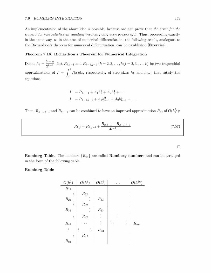
7.9. ROMBERG INTEGRATION 355
An implementation of the above idea is possible, because one can prove that the error for the
trapezoidal rule satisfies an equation involving only even powers of h. Thus, proceeding exactly
in the same way, as in the case of numerical differentiation, the following result, analogous to
the Richardson’s theorem for numerical differentiation, can be established [Exercise].
Theorem 7.16. Richardson’s Theorem for Numerical Integration
Define hk =b− a
2k−1. Let Rk,j−1 and Rk−1,j−1 (k = 2, 3, . . . , h; j = 2, 3, . . . , k) be two trapezoidal
approximations of I =
∫ b
af(x)dx, respectively, of step sizes hk and hk−1 that satisfy the
equations:
I = Rk,j−1 +A1h2k +A2h
4k + . . .
I = Rk−1,j−1 +A1h2k−1 +A2h
4k−1 + . . .
Then, Rk−1,j−1 and Rk,j−1 can be combined to have an improved approximation Rkj of O(h2jk ):
Rk,j = Rk,j−1 +Rk,j−1 −Rk−1,j−1
4j−1 − 1(7.57)
�
Romberg Table. The numbers {Rkj} are called Romberg numbers and can be arranged
in the form of the following table.
Romberg Table
O(h2) O(h4) O(h6) . . . O(h2n)
R11
〉 R22
R21 〉 R33
〉 R32
R31 〉 R43
〉 R42...
. . .
R41 · · · .... . . 〉 Rnn
...... 〉 Rn3
〉 Rn2
Rn1
356CHAPTER 7. NUMERICAL DIFFERENTIATION AND NUMERICAL INTEGRATION
A Recursive Relation for the 1st Column of the Romberg Table
The entries R11, R21, . . . , Rn1 of the 1st column of the Romberg table are just trapezoidal
approximations with spacing h1, h2, . . . , hn, respectively. These numbers can be computed by
using the composite trapezoidal rule. However, once R11 is computed, the other entries can be
computed recursively, as shown below, without repeatedly applying the composite trapezoidal
rule with increasing intervals.
R11 = Trapezoidal rule approximation with 1 interval:
R11 =h12[f(a) + f(b)] =
b− a
2[f(a) + f(b)].
R21 = Trapezoidal rule with 2 intervals:
R21 = h2
2 [f(a) + f(b) + 2f(a+ h2)]
= h2
2
[f(a) + f(b) + 2f
(a+ b−a
2
)]
= b−a4
[f(a) + f(b) + 2f
(a+ b−a
2
)]
It is easily verified that R21 can be written in terms of R11 as follows:
R21 =1
2[R11 + h1f(a+ h2)]
Similarly, R31 =12 [R21 + h2[f(a+ h3) + f(a+ 3h3)]
The trend is now clear. In general, we can write [Exercise]:
Rk1 =1
2[Rk−1,1 + hk−1[f(a+ hk) + f(a+ 3hk) + · · · + f(a+ (2k−1 − 1)hk)]].
=1
2
Rk−1,1 + hk−1
2k−2
∑
i=1
f(a+ (2i− 1)hk)
.
(7.58)
Constructing the Romberg Table
The Romberg table can be generated row-by-row as shown below:
The 1st row:
R11 =1
2[(b− a)(f(a) + f(b))].

7.9. ROMBERG INTEGRATION 357
The 2nd row:
(i) Compute R21 by setting k = 1 in (7.58):
R21 =1
2[R11 + h1f(a+ h2)].
(ii) Compute R22 by combining R11 and R21 using (7.57):
R22 = R21 +R21 −R11
3.
The 3rd row:
(i) Compute R31 by setting k = 3 in (7.58):
R31 =1
2[R21 + h2(f(a+ h3) + f(a+ 3h3))].
(ii) Compute R32 by combining R21 and R31 using (7.57):
R32 = R31 +R31 −R21
3.
(iii) Compute R33 by combining R22 and R32 using (7.57):
R33 = R32 +R32 −R22
15.
In general, compute the kth row as:
(i) Compute Rk1 from Rk−1,1 using (7.58):
Rk1 =1
2
Rk−1,1 + hk−1
2k−2
∑
i=1
f(a+ (2i− 1)hk)
.
(ii) Compute Rk2, Rk3, . . . , Rkk using (7.57):
Rkj = Rk,j−1 +Rk,j−1 −Rk−1,j−1
4k−1 − 1, j = 2, 3, . . . , k.
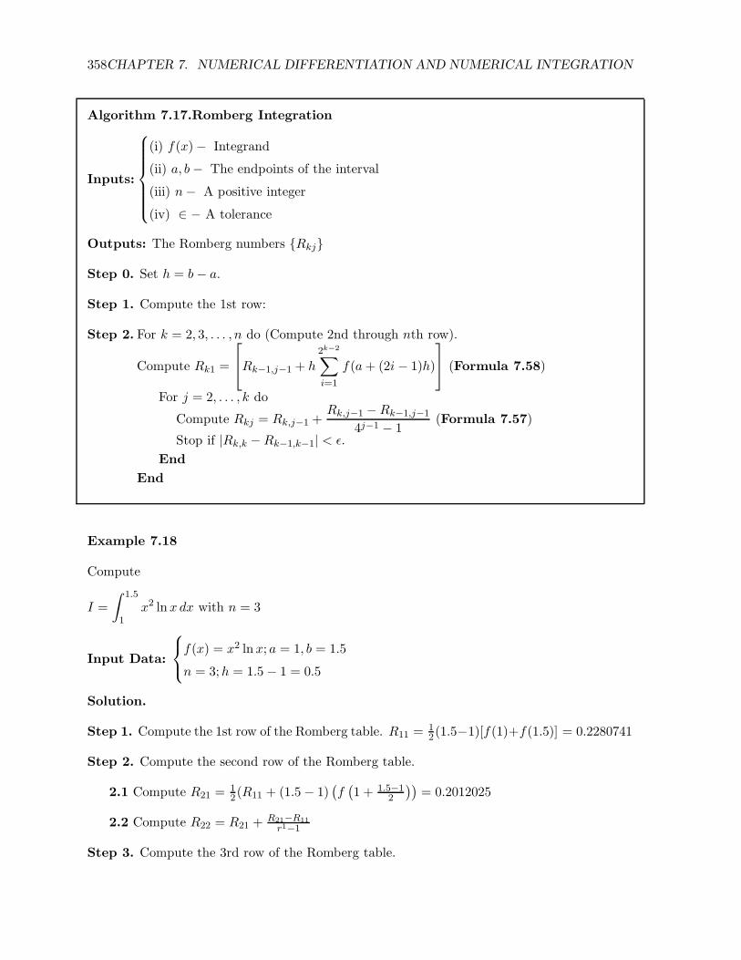
358CHAPTER 7. NUMERICAL DIFFERENTIATION AND NUMERICAL INTEGRATION
Algorithm 7.17.Romberg Integration
Inputs:
(i) f(x)− Integrand
(ii) a, b− The endpoints of the interval
(iii) n− A positive integer
(iv) ∈ − A tolerance
Outputs: The Romberg numbers {Rkj}
Step 0. Set h = b− a.
Step 1. Compute the 1st row:
Step 2. For k = 2, 3, . . . , n do (Compute 2nd through nth row).
Compute Rk1 =
Rk−1,j−1 + h2k−2
∑
i=1
f(a+ (2i − 1)h)
(Formula 7.58)
For j = 2, . . . , k do
Compute Rkj = Rk,j−1 +Rk,j−1 −Rk−1,j−1
4j−1 − 1(Formula 7.57)
Stop if |Rk,k −Rk−1,k−1| < ǫ.
End
End
Example 7.18
Compute
I =
∫ 1.5
1x2 lnx dx with n = 3
Input Data:
f(x) = x2 lnx; a = 1, b = 1.5
n = 3;h = 1.5 − 1 = 0.5
Solution.
Step 1. Compute the 1st row of the Romberg table. R11 =12(1.5−1)[f(1)+f(1.5)] = 0.2280741
Step 2. Compute the second row of the Romberg table.
2.1 Compute R21 =12(R11 + (1.5− 1)
(f(1 + 1.5−1
2
))= 0.2012025
2.2 Compute R22 = R21 +R21−R11
r1−1
Step 3. Compute the 3rd row of the Romberg table.
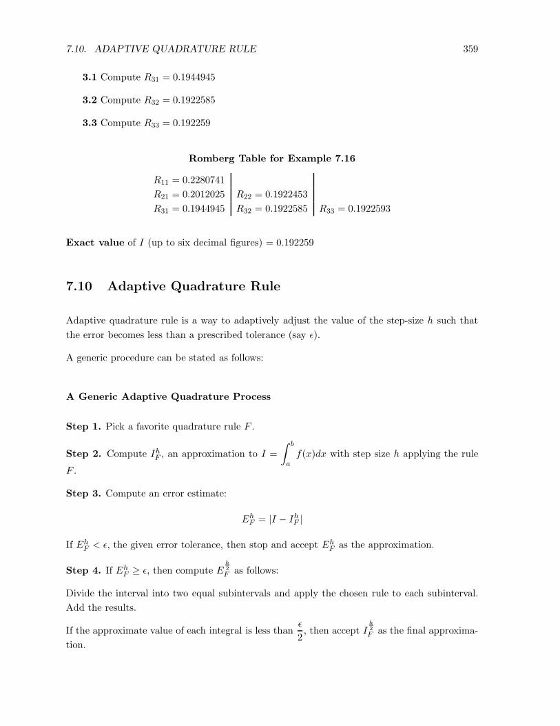
7.10. ADAPTIVE QUADRATURE RULE 359
3.1 Compute R31 = 0.1944945
3.2 Compute R32 = 0.1922585
3.3 Compute R33 = 0.192259
Romberg Table for Example 7.16
R11 = 0.2280741
R21 = 0.2012025 R22 = 0.1922453
R31 = 0.1944945 R32 = 0.1922585 R33 = 0.1922593
Exact value of I (up to six decimal figures) = 0.192259
7.10 Adaptive Quadrature Rule
Adaptive quadrature rule is a way to adaptively adjust the value of the step-size h such that
the error becomes less than a prescribed tolerance (say ǫ).
A generic procedure can be stated as follows:
A Generic Adaptive Quadrature Process
Step 1. Pick a favorite quadrature rule F .
Step 2. Compute IhF , an approximation to I =
∫ b
af(x)dx with step size h applying the rule
F .
Step 3. Compute an error estimate:
EhF = |I − IhF |
If EhF < ǫ, the given error tolerance, then stop and accept Eh
F as the approximation.
Step 4. If EhF ≥ ǫ, then compute E
h
2
F as follows:
Divide the interval into two equal subintervals and apply the chosen rule to each subinterval.
Add the results.
If the approximate value of each integral is less thanǫ
2, then accept I
h
2
F as the final approxima-
tion.
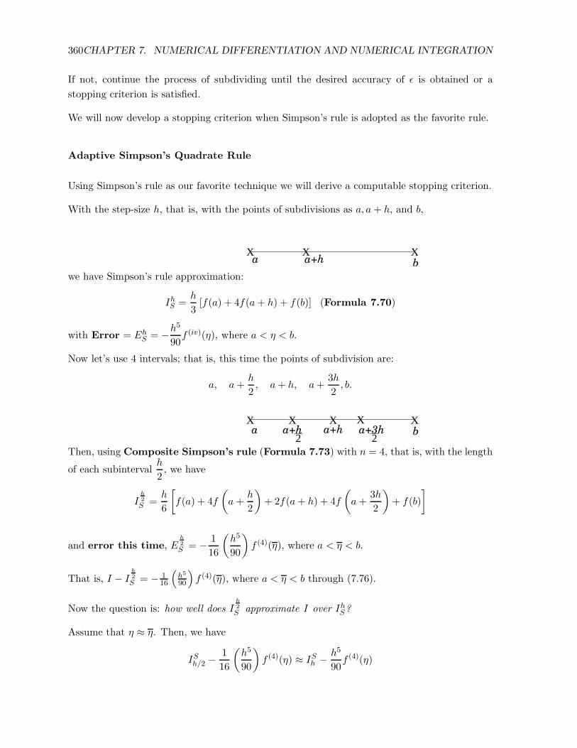
360CHAPTER 7. NUMERICAL DIFFERENTIATION AND NUMERICAL INTEGRATION
If not, continue the process of subdividing until the desired accuracy of ǫ is obtained or a
stopping criterion is satisfied.
We will now develop a stopping criterion when Simpson’s rule is adopted as the favorite rule.
Adaptive Simpson’s Quadrate Rule
Using Simpson’s rule as our favorite technique we will derive a computable stopping criterion.
With the step-size h, that is, with the points of subdivisions as a, a+ h, and b,
X XXa a+h b
we have Simpson’s rule approximation:
IhS =h
3[f(a) + 4f(a+ h) + f(b)] (Formula 7.70)
with Error = EhS = −h
5
90f (iv)(η), where a < η < b.
Now let’s use 4 intervals; that is, this time the points of subdivision are:
a, a+h
2, a+ h, a+
3h
2, b.
X Xb
X X Xa+ha a+h
2a+3h
2Then, using Composite Simpson’s rule (Formula 7.73) with n = 4, that is, with the length
of each subintervalh
2, we have
Ih
2
S =h
6
[
f(a) + 4f
(
a+h
2
)
+ 2f(a+ h) + 4f
(
a+3h
2
)
+ f(b)
]
and error this time, Eh
2
S = − 1
16
(h5
90
)
f (4)(η), where a < η < b.
That is, I − Ih
2
S = − 116
(h5
90
)
f (4)(η), where a < η < b through (7.76).
Now the question is: how well does Ih
2
S approximate I over IhS?
Assume that η ≈ η. Then, we have
ISh/2 −1
16
(h5
90
)
f (4)(η) ≈ ISh − h5
90f (4)(η)
7.10. ADAPTIVE QUADRATURE RULE 361
orh5
90f (4)(η) ≈ 16
15[IhS − Ih/2s ].
From (7.76), we then have
|I − Ih/2s | ≈ 1
15|IhS − I
h/2S | (7.59)
This is a rather pleasant result, because it is easy to compute∣∣IhS − I
h
2
S
∣∣. Suppose this quantity
is denoted by δ.
Then, if we choose h such that δ = 15ǫ, we see that∣∣E
h
2
S
∣∣ < ǫ.
Thus a stopping criterion for the adaptive Simpson’s rule will be:
Stop the process of subdivision as soon as the
1
15
∣∣IhS − I
h
2
S
∣∣ < ǫ. (7.60)
Example 7.19
Approximate
∫ π
2
0cos xdx using Simpson’s adaptive quadrature rule with an accuracy of ǫ =
10−3.
Step 1. Simpson’s rule approximation with two intervals.
Input Data: f(x) = cos x; a = 0, b = π2 ;h = π
4 .
x0 = a = 0, x1 = π4 , x2 = b = π
2 .
Formula to be used: IhS = h3
[f(a) + 4f
(a+b2
)+ f(b)
].
IhS =π
12
[
f(0) + 4f(π
4
)
+ f(π
2
)] (
Note that h =π
4
)
.
=π
12
[
cos(0) + 4 cos(π
4
)
+ cos(π
2
)]
= 1.0023
Step 2. Simpson’s rule approximation with four intervals.
Input Data: f(x) = cos x; a = 0, b = π2 .
x0 = a = 0, x1 = π8 , x2 = π
4 , x3 =3π8 , x4 = b = π
2 .
362CHAPTER 7. NUMERICAL DIFFERENTIATION AND NUMERICAL INTEGRATION
Formula to be used:
Ih
2
S =π4
6
[
f(0) + 4f(π
8
)
+ 2f(π
4
)
+ 4f
(3π
8
)
+ f(π
2
)]
=π
24
[
cos(0) + 4 cos(π
8
)
+ 2cos(π
4
)
+ 4cos
(3π
8
)
+ cos(π
2
)]
= 1.0001
Now1
15
∣∣∣∣IhS − I
h
2
S
∣∣∣∣= 1.4667 × 10⁻⁴. Since ǫ = 10−3, we can stop.
Note the actual error is∣∣∣∣
∫ b
af(x)dx− I
h
2
S
∣∣∣∣= 10−4
7.11 Gaussian Quadrature
So far, we have discussed the quadrature rules of the form:
∫ b
af(x)dx ≈ w0f(x0) + w1f(x1) . . . + wn−1f(xn−1), (7.61)
where the numbers x0, x1, . . . , xn−1, called nodes, are given, and the numbers, w0, . . . , wn−1,
called weights, are determined by a quadrature rule.
For example, in
• Trapezoidal Rule:
∫ b
af(x)dx ≈ h
2[f(x1)+ f(x2)] =
h
2f(x0)+
h
2f(x1), the nodes x0 and x1
are specified and the weights w0 = w1 =h2 are determined by the rule.
In fact, recall that in this case, w0 = w1 =h2 are determined as follows:
w0 =
∫ x1
x0
x− x1x0 − x1
dx =x1 − x0
2=h
2
w1 =
∫ x1
x0
x− x0x1 − x0
dx =x1 − x0
2=h
2
• Simpson’s Rule:
∫ b
af(x)dx ≈ h
3[f(x1) + 4f(x1) + f(x2)] =
h
3f(x0) +
4h
3f(x1) +
h
3f(x2).
The nodes x0, x1, and x2 are specified and the weights w1 = w3 =h3 and w2 =
4h3 are determined
by Simpson’s rule.

7.11. GAUSSIAN QUADRATURE 363
It is natural to wonder if we can devise a quadrature rule by determining both the nodes and
the weights. The idea is to obtain a quadrature rule that is exact for all polynomials of degree
less than or equal to 2n − 1, which is the largest class of polynomials for which one can hope
for the rules to be exact. This is because, we have 2n parameters: n nodes and n weights
and a polynomial of degree 2n − 1 can contain at most 2n parameters. The process is known
as Gaussian Quadrature rule.
7.11.1 Derivation of Gaussian Quadrature Rule
We first derive this rule in the simple cases when n = 2 and n = 3 with the interval [−1, 1].
Case n=2. Here the abscissas is x0 and x1. The weights w0 and w1 are to be found such that
the rule will be exact for all polynomials of degree less than or equal to 3.
Since the polynomials 1, x, x2, and x3 form a basis of all polynomials of degree less than or
equal to 3, we can set f(x) = 1, x, x2 and x3 successively in the formula (7.61) to determine w0
and w1.
• f(x) = 1:
∫ 1
−11 dx = w0f(x0) + w1f(x1) or 2 = w0 + w1.
• f(x) = x:
∫ 1
−1x dx = w0f(x0) + w1f(x1) or 0 = w0x0 + w1x1.
• f(x) = x2:
∫ 1
−1x2 dx = w0f(x0) + w1f(x1) or
23 = w0x
20 + w1x
21.
• f(x) = x3:
∫ 1
−1x3 dx = w0f(x0) + w1f(x1) or 0 = w0x
31 + w1x
31.
Thus, we have the following systems of nonlinear equations to solve:
w0 + w1 = 2
w0x0 +w1x1 = 0
w0x20 +w1x
21 = 2
3
w0x30 +w1x
31 = 0
(7.62)
A solution of this system of equations is
w0 = w1 = 1;x0 = − 1√3, x1 =
1√3.
Thus, for n = 2, we have the 2-point Gaussian Quadrature rule
364CHAPTER 7. NUMERICAL DIFFERENTIATION AND NUMERICAL INTEGRATION
∫ 1
−1f(x)dx ≈ f
(
− 1√3
)
+ f
(1√3
)
.
Case n=3. Here we seek to find x0, x1, and x2; and w0, w1, and w2 such that the rule will be
exact for all polynomials of degree up to five (note that n = 3; so 2n − 1 = 5).
Taking f(x) = 1, x, x2, x3, x4, and x5, and proceeding exactly as above, we can show [Exercise]
that the following systems of equations are obtained:
w0 + w1 + w2 = 2
w0x0 + w1x1 + w2x2 = 0
w0x20 + w1x
21 + w2x
22 =
2
3
w0x30 + w1x
31 + w2x
32 = 0
w0x40 + w1x
41 + w2x
42 =
2
5
w0x50 + w1x
51 + w2x
52 = 0
(7.63)
The above nonlinear system is rather difficult to solve. However, it turns out that the system
will be satisfied if x0, x1, and x2 are chosen as the roots of an orthogonal polynomial, called
Legendre polynomial and with this particular choice of x’s, the weights, w0, w1, and w2 are
computed as
wi =
∫ 1
−1Li(x)dx, i = 0, 1, 2
where Li(x) is the ith Lagrange polynomial of degree 3. This is also true for n = 2, and in fact
for any n, as the following discussions show.
7.11.2 Determining Nodes and Weights via Legendre Polynomials
We have encountered the notion of orthogonal polynomials in Chapter 6 in the context of
interpolation with the zeros of the orthogonal Chebyshev polynomial. Recall that when the
Chebyshev zeros are used as the nodes of interpolation, the error can be substantially reduced.
Here we show that the zeros of another orthogonal polynomial, called the Legendre polyno-
mial, plays a vital role in Gaussian quadrature. We first remind the readers of the definition
of an orthogonal polynomial.
A polynomial Pn(x) of degree n is an orthogonal polynomial with respect to the weight
function w(x) in [a, b] if, for each polynomial Pm(x) of degree m < n,
7.11. GAUSSIAN QUADRATURE 365
∫ b
aw(x)Pn(x) Pm(x)dx = 0
We will discuss more about orthogonal polynomials later in Chapter 10.
As in the case of Chebyshev polynomials, the Legendre polynomials can also be generalized
recursively.
Recursion to generate Legendre polynomials
Set P0(x) = 1, P1(x) = x.
Then, the Legendre polynomials {Pk(x)} can be generated from the recursive relation:
Pk+1(x) =(2k + 1)xPk(x)− kPk−1(x)
k + 1, k = 1, 2, 3, . . . , n.
Thus,
k=1: P2(x) =3xP1(x)− P0(x)
2= 3
2x2 − 1
2 . (Legendre polynomial of degree 2)
k=2: P3(x) =52
(x3 − 3
5x). (Legendre polynomial of degree 3)
and so on.
Choosing the Nodes and Weights
The following theorem shows how to choose the nodes x0, x1, . . . , xn−1 and the weights w0, w1, . . . , wn−1
such that the quadrature formula
n−1∑
i=0
wif(xi) is exact for all polynomials of degree less than or
equal to 2n− 1.
Theorem 7.20. (Choosing the Nodes and Weights in n-point Gaussian Quadrature)
Let
(i) the nodes x0, x1, . . . , xn−1 be chosen as the n-zeros of the nth degree Legendre polynomial
Pn(x) of degree n.
(ii) the weights w0, w1, . . . , wn−1 be defined by
wi =
∫ 1
−1Li(x)dx, i = 0, . . . , n− 1
366CHAPTER 7. NUMERICAL DIFFERENTIATION AND NUMERICAL INTEGRATION
where Li(x) is the ith Lagrange polynomial, each of degree (n− 1), given by:
Li(x) =
n−1∏
j=1
(x− xj)
xi − xj. j 6= i (7.64)
Then
for any polynomial P (x) of degree at most (2n − 1), we have
∫ 1
−1P (x)dx =
n−1∑
i=0
wiP (xi). (7.65)
Proof. Case 1: First, assume that P (x) is a polynomial of degree at most n− 1. Write P (x)
as:
P (x) = L0(x)P (x0) + L1(x)P (x1) + · · ·+ Ln−1(x)P (xn−1), (7.66)
where x0, x1, . . . , xn−1 are the zeros of the Legendre polynomial of degree n. This representation
is exact, since the error term
P (n)(ξx)(x− x0) . . . (x− xn−1)
is zero by virtue of the fact that the n-th derivative P (n)(x) of P (x), which is a polynomial of
degree at most n− 1, is zero.
So, integrating (7.84) from a = −1 to a = 1 and noting that P (xi), i = 0, . . . , n−1 are constants,
we obtain∫ 1
−1P (x)dx = P (x0)
∫ 1
−1L0(x)dx+ P (x1)
∫ 1
−1L1(x)dx+ · · ·+ P (xn−1)
∫ 1
−1Ln−1(x)dx
=
n−1∑
i=0
wi(x)P (xi).
Remembering that wi =
∫ 1
−1Li(x)dx, i = 0, . . . , n− 1, the above equation becomes
∫ 1
−1P (x)dx = w0P0(x) + wiP1(x) + · · ·+ wn−1Pn−1(x).
Case 2: Next, let’s assume that the degree of P (x) is at most 2n − 1, but at least n. Then
P (x) can be written in the form:
7.11. GAUSSIAN QUADRATURE 367
P (x) = Qn−1(x)Pn(x) +Rn−1(x) (7.67)
where Pn(x) is a nth-degree Legendre polynomial and Qn−1(x) and Rn−1(x) are polynomials
of degree at most n− 1. Substituting x = xi in (7.85), we get
P (xi) = Qn−1(xi)Pn(xi) +Rn−1(xi)
Since xi are the zeros of Pn(x), Pn(xi) = 0. Thus, P (xi) = Rn−1(xi).
From (7.85), we have∫ 1
−1P (x)dx =
∫ 1
−1Qn−1(x)Pn(x)dx+
∫ 1
−1Rn−1(x)dx
By the orthogonal property of the Legendre polynomial Pn(x),
∫ 1
−1Qn−1(x)Pn(x)dx = 0.
So,
∫ 1
−1P (x)dx =
∫ 1
−1Rn−1(x)dx.
Again, since Rn−1(x) is a polynomial of degree at-most n− 1, we can write, by Case I:
∫ 1
−1Rn−1(x)dx =
n−1∑
i=0
wiRn−1(xi)
Thus,∫ 1
−1P (x)dx =
n−1∑
i=0
wiRn−1(xi) =
n−1∑
i=0
wiP (xi).
Gauss-Legendre n-point Rule
Step 1. Pick n
Step 2. Compute the n zeros, x0, x1, . . . , xn−1 of the nth degree Legendre polynomial.
Step 3. Compute the corresponding weights:
wi =
∫ 1
−1Li(x)dx , i = 0, 1 . . . , n− 1
where wi is the ith Lagrange polynomial.

368CHAPTER 7. NUMERICAL DIFFERENTIATION AND NUMERICAL INTEGRATION
Step 4. Compute the integral approximation:
InGL = w0f(x0) + w1f(x1) + · · ·+ wn−1f(xn−1).
Remarks: The zeros of the Legendre polynomials and the corresponding weights are often
available from a table.
Working with an arbitrary interval [a,b]: So far our discussion on Gaussian quadrature
has been to approximate
∫ 1
−1f(x)dx.
If we need to approximate
∫ b
af(x) by Gaussian quadrature, we must transform the interval
[a, b] into [−1, 1] as follows:
Substitute
x =1
2[(b− a)t+ a+ b].
Then
dx =b− a
2dt.
∫ b
af(x)dx =
∫ 1
−1f
((b− a)t
2+ a+ b
)(b− a)
2dt
Thus, to approximate I =∫ ba f(x) using Gauss-Quadrature rule, do the following:
Step 1. Transform the integral∫ ba f(x)dx to b−a
2
∫ 1−1 f
((b−a)t
2 + a+ b)
dt = b−a2
∫ 1−1 F (t)dt .
Step 2. Apply n-point Gauss-Quadrature rule to∫ 1−1 F (t)dt.
Step 3. Multiply the result from Step 2 by b−a2 to approximate I.
Error in n-point Gaussian Quadrature: It can be shown that the error in n-point Gaus-
sian quadrature is given by
EnC =
f (2n)(ξx)
2n!
∫ b
a[ψ(x)]2dx
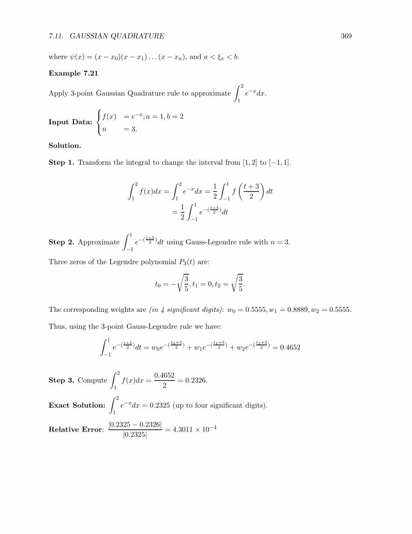
7.11. GAUSSIAN QUADRATURE 369
where ψ(x) = (x− x0)(x− x1) . . . (x− xn), and a < ξx < b.
Example 7.21
Apply 3-point Gaussian Quadrature rule to approximate
∫ 2
1e−xdx.
Input Data:
f(x) = e−x; a = 1, b = 2
n = 3.
Solution.
Step 1. Transform the integral to change the interval from [1, 2] to [−1, 1].
∫ 2
1f(x)dx =
∫ 2
1e−xdx =
1
2
∫ 1
−1f
(t+ 3
2
)
dt
=1
2
∫ 1
−1e−( t+3
2)dt
Step 2. Approximate
∫ 1
−1e−( t+3
2)dt using Gauss-Legendre rule with n = 3.
Three zeros of the Legendre polynomial P3(t) are:
t0 = −√
3
5, t1 = 0, t2 =
√
3
5.
The corresponding weights are (in 4 significant digits): w0 = 0.5555, w1 = 0.8889, w2 = 0.5555.
Thus, using the 3-point Gauss-Legendre rule we have:
∫ 1
−1e−( t+3
2)dt = w0e
−(t0+3
2) + w1e
−(t1+3
2) +w2e
−(t2+3
2) = 0.4652
Step 3. Compute
∫ 2
1f(x)dx =
0.4652
2= 0.2326.
Exact Solution:
∫ 2
1e−xdx = 0.2325 (up to four significant digits).
Relative Error:|0.2325 − 0.2326|
|0.2325| = 4.3011 × 10⁻⁴
370CHAPTER 7. NUMERICAL DIFFERENTIATION AND NUMERICAL INTEGRATION
7.12 Exercises on Part II
7.1. (Computational) Suppose x0 = 0, x1 = 1, and x2 = 2 are the three nodes and we are
required to find a quadrature rule of the form
∫ 2
0f(x)dx = w0f(0) + w1f(1) + w2f(2)
which should be exact for all polynomials of degree less than or equal to 2. What are w0,
w1, and w2?
7.2. (Computational) Suppose a quadrature rule of the form
∫ 1
0f(x)dx = w0f(0) + f(x1)
has to be devised such that it is exact for all polynomials of degree less than or equal to
1. What are the values of x1 and w0?
7.3. (Computational) Is it possible to devise a quadrature rule of the form
∫ 20
1f(x)dx =
w0f(1) + w1f(2) + w2f(3) + · · · + w19f(20) that is exact for all polynomials of as high
of a degree as possible? Determine why solving the system for the weights will not be
computationally effective.
7.4. (Computational) Using the appropriate data from Exercise 7.1 in (Exercises on Nu-
merical Differentiation),
A. Approximate the following integrals:
(i)
∫ 3
0sinxdx
(ii)
∫ 3
0cos xdx
(iii)
∫ 3
0xexdx
by each of the following quadrature rules:
(a) trapezoidal rule with h = 3.
(b) Simpson’s rule with h = 1.5.
(c) Simpson’s 38 th rule with h = 1.
(d) corrected trapezoidal rule with h = 3.
B. In each case (above), compute the maximum absolute error and compare these errors
with those obtained by the analytical formulas.
7.5. (Computational) Using the appropriate data of Exercise 7.2 in approximate the
following integrals,
(a)
∫ π
0
√x sinxdx
(b)
∫ π
0sin(sin sin(x))dx

7.12. EXERCISES ON PART II 371
(c)
∫ 2
0
[√x+
√
x+√x
]
dx
by each of the following rules:
(i) trapezoidal rule with h = π.
(ii) Simpson’s rule with h = h2 .
(iii) Boole’s rule with h = π4 .
7.6. (Analytical) Derive the trapezoidal and Simpson’s rule using Newton’s interpolation
with forward differences.
7.7. (Analytical)
(a) Derive Boole’s rule.
(b) Prove that Boole’s rule has a degree of precision of 5.
7.8. (Analytical) Derive Simpson’s 38th rule with error formula.
7.9. (Analytical) Drive the corrected trapezoidal rule with error formula.
7.10. Derive error formula for Simpson’s rule using Taylor’s Series of order 3 about x1.
7.11. (Computational) Using the appropriate data set of Exercise 1 in Section 7.3,
A. Approximate the following integrals:
(i)
∫ 3
0sinxdx
(ii)
∫ 3
0cos xdx
(iii)
∫ 3
0xexdx
by the
(a) composite trapezoidal rule with h = 0.5.
(b) composite Simpson’s rule with h = 0.5.
B. Compute the maximum absolute error in each case above, and compare the errors
with the actual absolute errors obtained by analytical rules.
C. For each of the integrals in part A, determine how the result obtained by the basic
rule compare with those by the composite rule?
7.12. () Determine h and N to approximate the integral
∫ 1
0e−t2dt within an accuracy of
G = 10−5 using the
(i) composite trapezoidal rule.

372CHAPTER 7. NUMERICAL DIFFERENTIATION AND NUMERICAL INTEGRATION
(ii) composite Simpson’s rule.
Which one is better and why?
7.13. True or False. The degree of precision of a quadrature rule is the degree of the interpo-
lating polynomial on which the rule is based. Explain your answer.
7.14. (a) Show that when Simpson’s rule is applied to
∫ 2π
0sinxdx, there is zero error, assum-
ing no round-off.
(b) Obtain a generalization to the other integrals
∫ b
af(x)dx. Show that Simpson’s rule
is exact for
∫ π
2
0cos2 xdx.
7.15. Prove that the quadrature rule of the form
∫ 3
1f(x)dx ≈ w0f(1) + w1f(2) + w2f(3) is
exact for all polynomials of as high a degree as possible, and is nothing but Simpson’s
rule.

7.13. MATLAB PROBLEMS ONNUMERICAL QUADRATURE AND THEIR APPLICATIONS373
7.13 MATLAB Problems on Numerical Quadrature and their
Applications
M7.1